*, Q HYDROLOGICAL PROCESSES, VOL. 5,59-79 (1991)

,3

THE PREDICTION OF HILLSLOPE FLOW PATHS FOR DISTRIBUTED HYDROLOGICAL MODELLING USING DIGITAL

TERRAIN MODELS

P. QUINN, K. BEVEN, Centre for Research oit Environinental Systems, Lancaster University, Lancaster, LAI 4YQ, U.K.

P. CHEVALLIER Bistituto de Pesquisas Hidraulicas, Universidade Federal do Rio Grande do Sol, CP 530, 90001 Porto Allegre RS,

Brasil AND

O. PLANCHON ORSTOM, Centre de Montpellier, 2051 Ave du Val de Montferraiid, 34032 Montpellier, France

ABSTRACT

The accuracy of the predictions of distributed hydrological models must depend in part on the proper specification of flow pathways. This paper examines some of the problems of deriving flow pathways from raster digital terrain data in the context of hydrological predictions using TOPMODEL. Distributed moisture status is predicted in TOPMODEL on the basis of spatial indices that depend on flow path definition. The sensitivity of this index to flow path algorithm and grid size is examined for the case where the surface topography is a good indicator of local hydraulic gradients. A strategy for the case where downslope subsurface flow pathways may deviate from those indicated by the surface topography is described with an example application.

KEY WORDS Digital terrain data Flow pathways Distributed hydrological models

INTRODUCTION

There are increasing requirements for predictive models of distributed hydrological processes, often to be the basis for further predictions of water quality, erosion, or the effects of different localized management strategies. Such predictions require that the distributed processes be represented accurately which, for any particular catchment area, will depend upon the details of the model structure being used and also the way in which the catchment characteristics are defined. A critical catchment characteristic is catchment topography, which will generally have a major control over flow pathways for surface and near surface flow processes. Most distributed catchment models require some topographic input, and many require that downslope flow pathways be defined a priori on the basis of catchment topography. The analysis of catchment topography by manual methods can be tedious in the extreme, but the increasing availability of detailed digital terrain data opens up the option for automatic derivation of flow pathways from a terrain model of the catchment.

Three types of terrain data might be available in computer compatible form: digitized contour data; point elevation data on an irregular grid forming a Triangular Irregular Network (TIN); and point elevation data on a regular grid. The derivation of flow pathways directly from contour data has been addressed by O’Loughlin (1986), from TIN data by Gandoy-Bernasconi and Palacios-Velex (1990), and from regular data by Band (1986), Morris and Heerdegen (1988), and others. This paper is concerned with the use of regular gridded data. A detailed digital terrain model with 50 m grid will be available for the U.K. in the future, raising the question of how best to make use of such data for hydrological purposes.

0885-6087/91/010059-21$10.50 0 1991 by John Wiley & Sons, Ltd. Received and accepted 12 October 1990

er;sTo~ ~ o n d s Doctimzntaire

NO i 34.6+6 P ) C ~

60 P. QUI” ET AL.

An accurate distributed model must reflect not only the proper flow pathway for a water particle falling on any point in the catchment, but also the spatial and temporal variations in flow velocity taken by that particle on its route to the catchment outlet. In general, both flow pathways and velocities will be functions of the flow dynamics, reflecting the developing pattern of internal states of the system as well as the spatial and temporal variability in catchment characteristics such as hydraulic conductivities or flow resistances. While it is clear that it will never be possible to characterize the internal dynamics completely, it remains a research question as to what are the most important factors to take into account in distributed models. For catchment responses dominated by surface and near surface flow processes, topography might be expected to give a good indication of the gravitational potentials involved and might therefore s rve as a useful basis for modelling the spatial variability in both flow pathways and velocities. A number f distributed hydrological models in the past have used topography in this way, including kinematic overla ~d flow models (e.g. Smith and Woolhiser, 1971; Ross et al., 1979), kinematic subsurface flow models (e.g. Be en, 1982); TOPMODEL (e.g. Beven and Kirkby, 1979; Beven and Wood, 1983; Beven 1986,1987; Quinn et al., 1990), and the model of Moore et al. (1986).

There is however a question as to how well digital terrain model can represent the hydrological significant features of a catchment. This question is addressed here, within a TOPMODEL framework using an example data set from the Booro-Borotou catchment in the Côte d’Ivoire (Chevallier, 1990).

I DIGITAL TERRAIN ANALYSIS AND FLOW PATHWAYS

The most difficult part of digital terrain analysis is the creation of the digital terrain model itself. A raster elevation grid generally requires interpolation from irregular point elevations. Such data filling techniques can lead to a number of spurious topographic features, the most commonly mentioned being ‘sink’ features (Band 1986; Morris and Heerdegen, 1988). Equally important data anomalies are ‘dam’ features that are created either where interpolated values are artificially raised above the actual ‘true’ surface, or where the grid scale is too coarse to resolve local incised channel features. Such ‘dams’ an generate an upstream reservoir of sinks. These important problems are not addressed here and it is assu ed that the data sets being

created from a detailed ground survey by ORSTOM, Montpellier, France with a g id spacing of 12.5 metres. With this data set, three problems will be addressed. Thle Booro-Borotou da a set contains distinctive

features that associated fieldwork suggests are important to the hydrological res i onse. The first problem is that of the appropriate resolution of the DTM required for thle prediction of hydrological responses. This will be examined by looking at the sensitivity of the predictions of flow characteristics to the coarseness of the grid used.

The second problem to be addressed is the sensitivity of the predictions to the flow pathway algorithm used. A direct comparison is made between an algorithm that allows multiple flow directions to exit from a single grid cell and the more common algorithm that utilizes only one flow direction to exit from each cell.

Finally, Booro-Borotou provides an example of a catchment where flow pathways and hydraulic gradients may be estimated from the surface topography only over part of the catchment, in the valley bottoms. Elsewhere in the catchment, a deeply weathered soil and deep water table mean that the surface topography may not be such a good indicator of flow pathways. An extension of the TOPMODEL concept will be described to handle the case of deeper subsurface flow pathways while retaining a simple distributed model structure.

used are reliable. The digital terrain model for the Booro-Borotou catchment u 4 ed in this paper has been

THE TOPMODEL CONCEPTS I TOPMODEL is not a fixed model structure but rather a collection of concepts f r distributed hydrological modelling to be used where they appear approporiate. There are two very si i ple ideas at the heart of TOPMODEL: that downslope subsurface flows can be adequately represented by a succession of steady- state water table Dositions, and that there is an exDonentia1 relationshir, between local storage (or water table

. DIGITAL TERRAIN MODELLING IV: HILLSLOPE FLOW PATHS 61

C I level) and downslope flow rate. A further assumption that has been made in all applications of the concepts to date is that the local hydraulic gradient can be approximated by the local ground surface slope (tanp) thereby requiring a detailed analysis of catchment topography but, as will be shown below, this assumption may be relaxed if necessary. Beven (1986) and Quinn et al. (1990) give further details of the theory that underlies the TOPMODEL concepts and show how spatial variability of soil characteristics can be incorporate into the calculations.

TOPMODEL is mathematically and parametrically simple and relies on the preprocessing of digital terrain data to calculate the catchment distribution function of a topographic index ln(u/tan/?) where a is the cumulative upslope area draining through a point (per unit contour length) and tanp is the slope angle at the point. The ln(a/tan/?) index reflects the tendency of water to accumulate at any point in the catchment (in terms of a) and the tendency for gravitational forces to move that water downslope (expressed in terms of tanp as an approximate hydraulic gradient). The calculated values of both a and tanp will depend upon the analysis of flow pathways from the DTM data and the grid resolution used. Most surface flow pathway analyses using gridded elevation data in the past have assigned a single flow direction (using either four or eight possible directions) based on the local direction of greatest slope (e.g. Band, 1986; Morris and Heerdegen, 1988). While this approach will be assymptotically accurate as the grid scale becomes finer (subject to any residual errors in the production of the raster DTM itself), with grid scales of 50 m or coarser, the single flow direction approach may give rise to local inaccuracies, particularly on divergent hillslopes. This paper describes an alternative multiple flow direction approach and compares the resultant cumulative area and ln(a/tanp) distributions with the single direction algorithm at different grid resolutions.

THE MULTIPLE FLOW DIRECTION ALGORITHM

The calculation of a in the In(a/tan/?) index requires an analysis of flow pathways to determine the total upslope area ( A ) entering a grid element, together with an effective contour length (L) orthogonal to the direction of flow, from which a = A/L. A local slope angle must also be calculated. In the single flow direction algorithm it is normal to assume that the contour length is equal to the grid square length and that the slope angle is the greatest slope angle for any downslope direction.

A more general formulation is provided by the algorithm used in the current study which allows the accumulated upslope area for any one cell is to be distributed amongst all downslope directions. The directions are split into cardinal and diagonal directions with area being able to contribute downhill in up to eight flow directions. All eight directions would be utilized at a local internal peak in the catchment. Figure 1 shows how each flow direction is weighted by a ‘contour’ length where L1 and L2 are lengths normal to the direction of flow. L1 and L2 have been subjectively chosen by the simple geometrical construct shown in Figure 1; other choices are clearly possible. The fraction of the area draining through each grid element to each downslope direction is also made proportional to the gradient of each downhill flow path, so that steeper gradients will naturally attract more of the accumulated area.

The calculations are made only for the downhill directions and the relative amount is then deduced from:

n

AA, = A(tan piLi)/ (tan pjLj) j = 1

where n is the total number of downhill directions, AA, is the amount passed onto the ith downhill cell, A is the total upslope area accumulated in the current cell, tan pi is the gradient (difference in elevation/distance between the elevation values) in the ith downhill directions, Li is the contour length of the ith direction either cardinal (Ll) or diagonal (L2).

If the common term is separated

62 P. QUI" ET AL.

A subsection of the DTM

AI

A 4 A3 A 2 A l and A3 are Cardinal (L l )

A2 and A4 are Diagonal (L2)

L1 = 0.5 * Grid Size

L2 = 0.354 * Grid Size

For an example grid size of 1 unit , angles a and b and length L3

are used to calculate L I and L2

LI

I

0.5

0.5 \

0.5 0.5

Figure 1. Flow partitioning using the multiple flow direction algorithm

Each individual direction now receives:

AA, = C tan ßiLi

It is currently assumed that the most representative local slope angle for any one cell should be a weighted sum of the same proportion:

Thus the actual value of altan ß for the current cell will be the total area draining through that cell acting across a contour length equal to the sum of the downhill contour lengths and divided by the weighted average tan ß value:

n

altanß = A/ Lj tan ß j = 1

Substituting for the tan ß value the summation of the Li terms will cancel out leaving:

n altan ß = A/ (tan ß jL j )

j = 1

This is the same as the term C, so that:

altan ß = C

and :

in(a/tan $) = In(C).

DIGITAL TERRAIN MODELLING IV: HILLSLOPE FLOW PATHS 1 : 63

This utilization of multiple flow directions will result in different ln(u/tan p) distributions to those calculated using single flow directions. These differences are likely to become more significant as the size of the grid cell is increased and the likelihood of significant curvature of contour lines within a cell increases. In essence the multiple flow direction algorithm is a simple and approximate form of subgrid scale flow pathway interpolation.

THE STUDY CATCHMENT

The Booro-Borotou catchment (1.36 km2) has been the subject of both field and modelling studies by ORSTOM hydrologists (Chevallier, 1990). The catchment lies in a humid savannah region with runoff being generated by a mixture of saturation excess flows and subsurface storm flows. Figure 2 shows the digital terrain data set for the catchment at a resolution of 12.5 m. Field experience suggested that this resolution might be sufficient to properly represent the effect of certain topographic features on the hydrology, in particular the central valley bottom and headwater hollow areas.

The multiple direction flow pathway algorithm and the 12.5 m data set were used to generate a base data set of cumulative area and ln(u/tan p) values for comparison with later analyses. Figure 3 shows the cumulative area map and Figure 4 the pattern of ln(u/tan p). The upper scale threshold of Figure 4 has been chosen to reflect the maximum extent of the commonly observed saturated area in the catchment.

SENSITIVITY TO FLOW PATHWAY ALGORITHM CHOICE

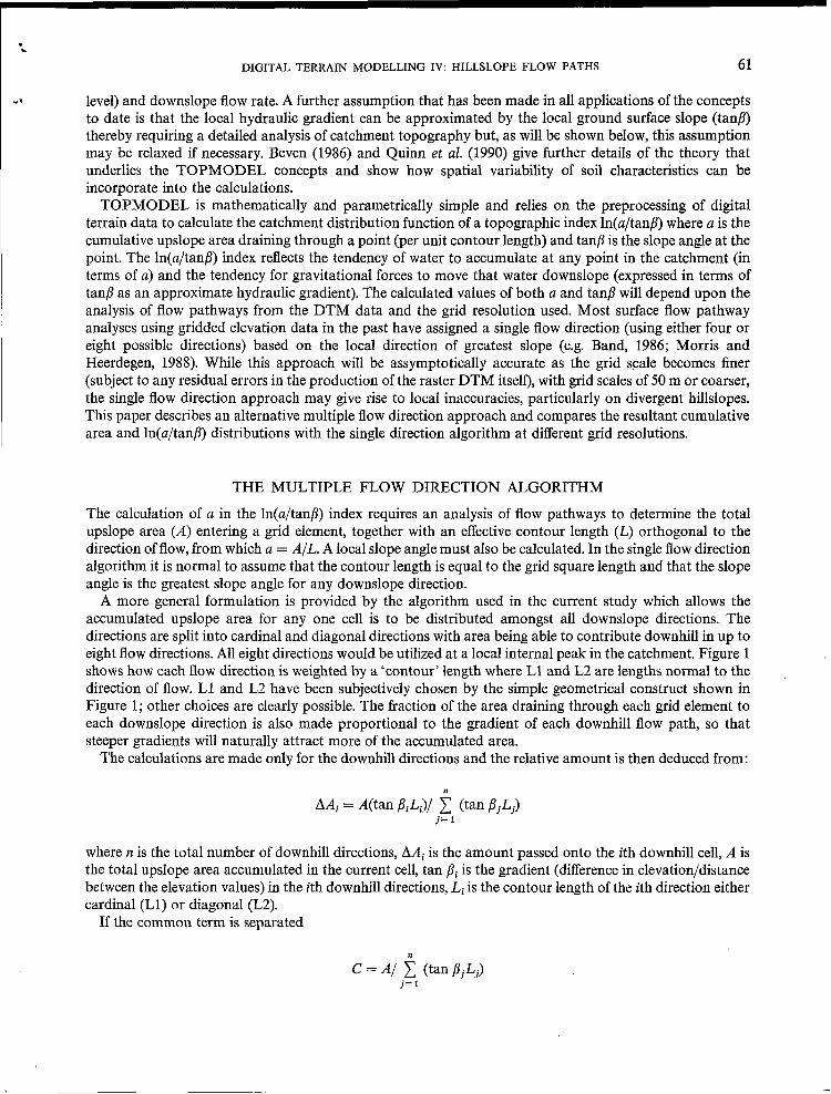
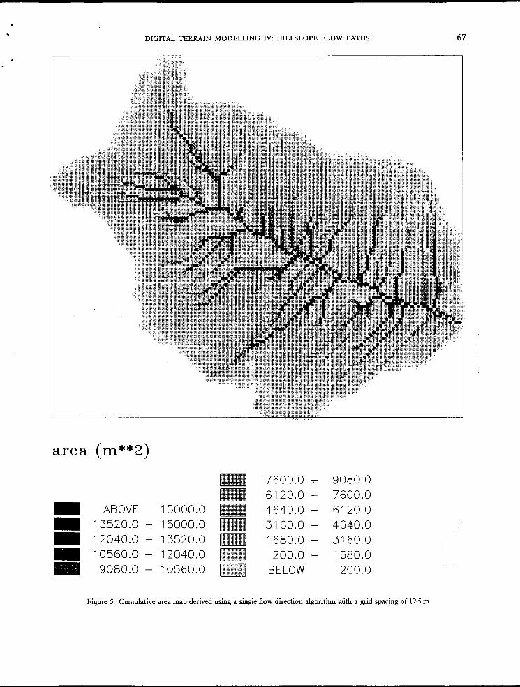
Figures 5 and 6 show the pattern of cumulative area and ln(u/tan p) values produced by the single flow pathway algorithm, using the same scale classes. It is readily apparent that the two algorithms give quite different patterns (and by implication different hydrological predictions). The downslope accumulation of area into the gullies and minor tributaries is much quicker, thus giving the impression that these channels have extended upslope. Once area has entered a flow path it cannot be later distributed as in the multiple flow direction algorithm, causing the resulting features to be much sharper in appearance and give a ‘banding’ effect. The multiple flow method gives a more realistic pattern of accumulating area on the hillslope portion of the catchment but once in the valley bottom tends to braid the cumulative area back and forth across the floodplain. The single flow direction algorithm is therefore more suitable once the flow has entered the more permanent drainage system. This suggests that the multiple flow direction method could be improved by overlaying the more permanent drainage system so that once hillslope flows reach a channel they remain there whilst being routed out of the catchment.

Figure 7 compares the cumulative distributions of ln(u/tanp) shown in Figures 4 and 6 for the two flow pathway algorithms. TOPMODEL uses the ln(u/tanp) distributions directly in the calculation of local saturation in the catchment. The two curves may be interpreted directly in terms of patterns of storage; in effect for the same set of model parameters a larger fractional area for a given ln(a/tan p) value suggests a greater predicted contributing area. The shape of the distribution function curves derived by the different algorithms are quite dissimilar. One cause of this difference is due to the single flow direction algorithm consistently giving higher values of tan fi, as the gradient utilized is always the steepest value and not an average of all downhill slope gradients.

SENSITIVITY TO THE DTM GRID SCALE

Distributed hydrological models have used a wide variety of grid scales and the choice of an appropriate scale is often controlled by economics or availability of data as well as the original modelling goals. If the modelling goal is the accurate representation of hillslope flow processes then the model should have an appropriate grid resolution. Clearly distributed modelling of hillslope flows will require a grid scale much smaller than the scale of the hillslope, but how much smaller? In the U.K. the choice of the resolution for the national database is 50 my so is this sufficient to model variable source area dynamics for example? The very

64 P. QUI" ET AL.

Elevation (m)

445.0 - 450.0 I I ABOVE 470.0 440.0 - 445.0 1-1 465.0 - 470.0 435.0 - 440.0

460.0 - 465.0 m 430.0 - 435.0 450.0 - 455.0 m BELOW 425.0 455.0 - 460.0 425.01 - 430.0

Figure 2. Digital Terrain Model for Booro-Borotou with a grid spacing of 12.5 m

. DIGITAL TERRAIN MODELLING IV: HILLSLOPE FLOW PATHS 65

area( m**Z) 7600.0 - 9080.0 6120.0 - 7600.0 m ABOVE 15000.0 4640.0 - 6120.0

0 13520.0 - 15000.0 3160.0 - 4640.0 12040.0 - 13520.0 1680.0 - 3160.0 m 10560.0 - 12040.0 200.0 - 1680.0 9080.0 - 10560.0 BELOW 200, o

Figure 3. Cumulative area map for Booro-Borotou with a grid spacing of 12.5 m

66 P. QUI" ET AL.

Ln (a/tan ß )

m E l m

ABOVE 11.2 - 10.4 - 9.6 - 8.8 -

12.0 12.0 11.2 10.4 9.6

8.0 7.2 6.4 5.6 4.8 4. O

BELOW

8.8 8.0 7.2 6.4 5.6 4.8 4.0

Figure 4. Ln(a/tan f i ) map for Booro-Borotou with a grid spacing of 12.5 m

DIGITAL TERRAIN MODELLING IV: HILLSLOPE FLOW PATHS 67

area (m**Z)

7600.0 - 9080.0 6120.0 - 7600.0 m ABOVE 15000.0 4640.0 - 6120.0

13520.0 - 15000.0 ~ 3160.0 - 4640.0 m 12040.0 - 13520,O ~ 1680.0 - 3160.0 10560.0 - 12040.0 200.0 - 1680.0 9080.0 - 10560.0 BELOW 200.0

Figure 5. Cumulative area map derived using a single flow direction algorithm with a grid spacing of 12.5 m

68 P. QUI” ET AL.

Ln (a/tan ß )

8.0 - 8.8 7.2 - 8.0 m ABOVE 12.0 6.4 - 7.2 m 11.2 - 12.0 5.6 - 6.4 m 10.4 - 11.2 4.8 - 5.6

9.6 - 10.4 4.0 - 4.8 8.8 - 9.6 BELOW 4.0

ml m’ Figure 6. Ln(a/tan p) map derived using a single flow direction algorithm, with a grid spacing of 12.5 m

1 .o

0.9

0.8

0.7

0.6 Q > 0.5 Q

0.4

0.3

0.2

o. 1

0.0

DIGITAL TERRAIN MODELLING IV: HILLSLOPE FLOW PATHS

Ln (a / tan ß ) value

69

3

Figure 7. Comparison of the single distribution function forms for the single and multiple flow direction algorithms

detailed data set for Booro-Borotou allows the sensitivity of the hydrological analysis to the grid scale to be examined.

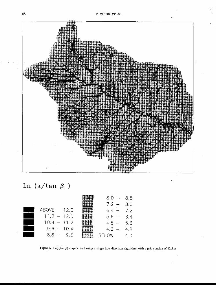
The resolution of the Booro-Borotou DTM was deteriorated to a grid scale of 50 m by reinterpolating the 1 metre contour data onto a coarser grid. The resulting DTM is shown in Figure 8, with the cumulative area and In(u/tan p) maps calculated using the multiple flow path algorithm in Figures 9 and 10. On first appearance these maps could be accepted as realistic, although considerable detail in the patterns has been lost, particularly in the definition of the smaller gulley-like flow lines.

This problem of smoothing across features that previously existed in the 12.5 m data is also reflected in the ln(u/tan p) index (Figure 10). Comparison of the area with values greater than 12, chosen as indicating the average saturated area, shows the area to be generally larger than with the 12.5 m data. Prediction of the overall dynamics of the soil moisture regime would also be expected to be different as can be shown by the comparison of the ln(u/tan p) distribution functions for the whole catchment (Figure 11). There is generally a higher percentage of higher ln(u/tan p) values in the catchment. This is partly due to the fact that very low values of ln(u/tan j?) can no longer exist due to the large increase in area of each grid cell. Once in the main drainage system, the flow pathways are contained within one or two cells in the valley bottom keeping these cumulative area values high but with little change in the calculated gradients.

Sensitivity to the grid resolution should not be ignored in the construction of models for larger catchments and global circulation models utilizing digital terrain data, where the temptation to compromise the resolution of the fundamental grid scale must also compromise the representation of crucial fundamental hydrological processes (such as the variable source area concept).

70 P. QUINN ET AL.

h

slevation (m) 450,O - 455.0 445.0 - 450.0 440.0 - 445.0

ABOVE 470.0 435.0 - 440.0 465.0 - 470.0 430.0 - 435.0 460.0 - 465.0 425.0 - 430.0 455.0 - 460.0 BELOW 425.0

Figure 8. Digital Terrain Model for Booro-Borotou with a grid spacing of 50 m

'

DIGITAL TERRAIN MODELLING IV: HILLSLOPE FLOW PATHS 71

Area (m**Z)

27500.0 - 32500.0 22500.0 - 27500.0

ABOVE 52500.0 17500.0 - 22500.0 47500.0 - 52500.0 12500.0 - 17500.0 42500.0 - 47500.0 7500.0 - 12500.0 37500.0 - 42500.0 2500.0 - 7500.0 32500.0 - 37500.0 BELOW 2500.0

Figure 9. Cumulative area map derived using a multiple flow direction algorithm applied to a grid spacing of 50 m

72 P. QUINN ET AL.

Ln (a/tan ,G )

8.0 - 8.8 7 .2 - 8.0

ABOVE 12.0 6.4 - 7 .2 11 .2 - 12 .0 5.6 - 6.4 10.4 - 11.2 4.8 - 5.6 9.6 - 10.4 4.0 - 4.8 8.8 - 9.6 BELOW 4.0

Figure 10. Ln(a/tan f i ) map derived using a multiple flow direction algorithm applied to a grid spacing of 50 m

(r . 1 .o

0.9

0.8

0.7

0.6 Q > 0.5 Q

0.4

0.3

0.2

o. 1

0.0

DIGITAL TERRAIN MODELLING IV: HILLSLOPE FLOW PATHS

PT - 12.5m

73

3

Ln (a/tan ,6 ) value

Figure 11. Comparison of the single distribution function forms for the 12.5 m and the 50 m data sets

SUBSURFACE FLOW PATH PHENOMENA

In the first part of this paper, it has been assumed that the downslope flow pathways of water could be determined on the basis of the surface topography, and that subsurface flow rates would be proportional to a hydraulic gradient approximately equal to the surface slope. Both assumptions underly the theory of the basic versions of TOPMODEL, but are clearly not always true. In cases where there is not a strong link between surface topography and subsurface flow, the question arises as to whether digital terrain data and TOPMODEL concepts might still be useful in modelling hydrological processes through some modification of the analyses. Such a situation is similar to that found in the Booro-Borotou catchment with its deeply weathered soil and deep saturated zone on the upper slopes, albeit with the additional complication of relatively impermeable lateritic crust horizons close to the surface over parts of the slopes (see Chevallier, 1990).

In such a case, the concept used by TOPMODEL clearly needs to be modified in a way that reflects more clearly the nature of the hydrological processes in such a catchment but does not compromise the advantages of simplicity in parameter calibration. This has been done in the present study by introducing the concept of a reference level with which to compare deviations in water table level. In the original TOPMODEL structure, this reference level is the soil surface everywhere in the catchment. This is not, a necessary assumption and the reference level can be allowed to depart from the soil surface to reflect the shape of the water table that might be expected in a catchment under quasi-steady flow conditions. Of course, the information with which to define such a reference level will not commonly be available and it may be necessary to invoke a degree of hydrological judgement. This is the case in the application to Booro-Borotou, where the field experience of the ORSTOM hydrologists has been used to define the reference level in the catchment.

74 P. QUI" ET AL. . In the Booro-Borotou catchment, the incised valley-bottom feature acts as a dynamic source area for

runoff during the wet season response of the catchment. The extent of this contributing area however appears to be mostly confined by the topography to the area adjacent to the mainstream (some 8-10 per cent of the catchment). Topography may be important in controlling the relationship between water table levels and runoff production in this area but elsewhere the water table departs from the soil surface and may lie deep within the deeply weathered soil. If a representative gradient of the water table surface can be estimated, given field experience, then that gradient can be used to define a new reference level to be used once the water table is no longer likely to intersect the soil surface under wet conditions. Where the water table is likely to intersect the surface, the surface elevation values are used to define the reference level as before. The difference in land surface elevation and reference level elevation can be used to obtain an estimate of storage and travel times in the unsaturated zone. Once the reference level has been defined for the whole catchment, it can be used within the TOPMODEL structure to derive the flow directions and ln(u/tan p) distribution in the same way as for a surface DTM.

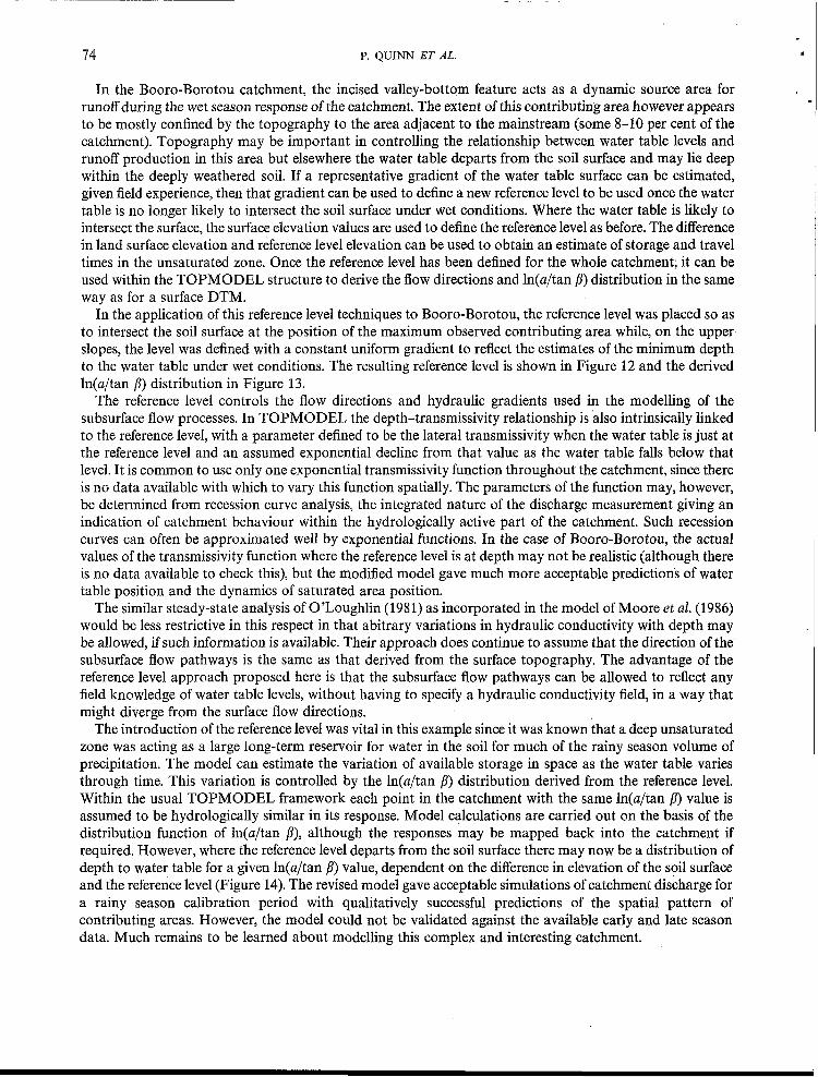
In the application of this reference level techniques to Booro-Borotou, the reference level was placed so as to intersect the soil surface at the position of the maximum observed contributing area while, on the upper slopes, the level was defined with a constant uniform gradient to reflect the estimates of the minimum depth to the water table under wet conditions. The resulting reference level is shown in Figure 12 and the derived ln(u/tan p) distribution in Figure 13.

The reference level controls the flow directions and hydraulic gradients used in the modelling of the subsurface flow processes. In TOPMODEL the depth-transmissivity relationship is also intrinsically linked to the reference level, with a parameter defined to be the lateral transmissivity when the water table is just at the reference level and an assumed exponential decline from that value as the water table falls below that level. It is common to use only one exponential transmissivity function throughout the catchment, since there is no data available with which to vary this function spatially. The parameters of the function may, however, be determined from recession curve analysis, the integrated nature of the discharge measurement giving an indication of catchment behaviour within the hydrologically active part of the catchment. Such recession curves can often be approximated well by exponential functions. In the case of Booro-Borotou, the actual values of the transmissivity function where the reference level is at depth may not be realistic (although there is no data available to check this), but the modified model gave much more acceptable predictions of water table position and the dynamics of saturated area position.

The similar steady-state analysis of O'Loughlin (1981) as incorporated in the model of Moore et al. (1986) would be less restrictive in this respect in that abitrary variations in hydraulic conductivity with depth may be allowed, if such information is available. Their approach does continue to assume that the direction of the subsurface flow pathways is the same as that derived from the surface topography. The advantage of the reference level approach proposed here is that the subsurface flow pathways can be allowed to reflect any field knowledge of water table levels, without having to specify a hydraulic conductivity field, in a way that might diverge from the surface flow directions.

The introduction of the reference level was vital in this example since it was known that a deep unsaturated zone was acting as a large long-term reservoir for water in the soil for much of the rainy season volume of precipitation. The model can estimate the variation of available storage in space as the water table varies through time. This variation is controlled by the In(u/tan p) distribution derived from the reference level. Within the usual TOPMODEL framework each point in the catchment with the same ln(u/tan /3) value is assumed to be hydrologically similar in its response. Model calculations are carried out on the basis of the distribution function of ln(u/tan p), although the responses may be mapped back into the catchment if required. However, where the reference level departs from the soil surface there may now be a distribution of depth to water table for a given ln(u/tan p) value, dependent on the difference in elevation of the soil surface and the reference level (Figure 14). The revised model gave acceptable simulations of catchment discharge for a rainy season calibration period with qualitatively successful predictions of the spatial pattern of contributing areas. However, the model could not be validated against the available early and late season data. Much remains to be learned about modelling this complex and interesting catchment.

c . '

DIGITAL TERRAIN MODELLING IV: HILLSLOPE FLOW PATHS 75

Elevation (m)

438.0 - 440.0 436.0 - 438.0

ABOVE 448.0 434.0 - 436.0 446.0 - 448.0 432.0 - 434.0 444.0 - 446.0 430.0 - 432.0 442.0 - 444.0 428.0 - 430.0 440.0 - 442.0 BELOW 428.0

Figure 12. A map of the form of the reference level throughout the catchment

76 P. QUINN ET AL.

Ln (a/tan ß )

10.0 - 11.0 9.0 - 10.0 m ABOVE 15.0 8.0 - 9.0 m 14.0 - 15.0 m 13.0 - 14.0 m 12.0 - 13.0

E 11.0 - 12.0

Figure 13. Ln(a/tan p) map calculated with the form of the rdference level as seen in Figure 12

.

Depth (m)

DIGITAL TERRAIN MODELLING IV: HILLSLOPE FLOW PATHS 77

ABOVE 19.8 17.6 15.4 13.2

22.0 22.0 19.8 17.6 15.4

11.0 8.8 6.6 4.4 2.2 0.0

BELOW

13.2 11.0 8.8 6.6 4.4 2.2 0.0

Figure 14. A map of the depth to the reference level from the surface topography showing the variability in available unsaturated zone storage across the catchment

a I 78 P. QUI” ET AL.

CONCLUSION

This paper has shown how topographical information can be used to reflect perceptions of variability of hydrological response of catchments, but also how great care and fundamental understanding of flow processes are necessary if digital terrain data are to be utilized properly in hydrological modelling. The TOPMODEL framework provides a parametrically simple method of utilizing digital terrain data to predict the changing patterns of water table and soil moisture status over time, but is dependent upon the validity of the quasi-steady flow assumptions and the derivation of an appropriate ln(a/tan a) distribution from the DTM data.

Three problems associated with the use of digital terrain data have been examined here: sensitivity to flow pathway algorithm, sensitivity to DTM grid scale, and the divergence of subsurface flow pathways from those indicated by the surface topography. It was shown that the grid resolution must reflect those features that are vital to the hydrological response and, as demonstrated for Booro-Borotou, this may be a finer scale than the 50 m scale commonly available. Both routing algorithm and the flow path algorithm may have an important effect on model predictions and, in particular, the pattern of predictions in space. While this may not necessarily result in less accurate predictions after model calibration, it must be expected that there will be an interaction between the grid scale used in the DTM analysis and the appropriate values of the parameters calibrated to a particular catchment area.

The problem of flow pathways and hydraulic gradients that may differ from those indicated by an analysis of the topography has been addressed and the idea of a reference level has been introduced. It has been shown that digital terrain data can still be of importance, both in controlling water table and contributing area dynamics in part of the catchment or in estimating storage and routing through the unsaturated zone. The concept of the reference level may be useful in other situations, for example in the study of underdrained catchments, or where soil depths increase downslopes. Clearly, in many cases the definition of an appropriate reference level with little field information available will be difficult and subjective. However, the possibility of assessing the resulting spatial patterns of predicted responses may prove more satisfactory than the blind application of an inappropriate model. It is an important aspect of this approach to modelling that such predictions can be compared with field perceptions of hydrological responses in their correct spatial context and, if necessary, modifications to the model structure made as part of the calibration procedure.

The concepts used in these modelling studies depend heavily upon an interaction between the modeller ’ and the field hydrologist and his perceptions, often qualitative, of the way in which a particular catchment responds. The studies of Booro-Borotou, in particular, greatly benefitted from the fieldwork carried out by ORSTOM scientists. Our future research will aim to make some of the possibilities for model structural definition directly accessible to the user with field experience as part of the calibration process.

I REFERENCES

Band, L. 1986. ‘Topographic partition of watersheds with digital elevation models’, Water Resour. Res., 22(1), 15-24. Beven, K. J. 1982. ‘On subsurface stormflow: predictions with simple kinematic theory for saturated and unsaturated flows’, Water

Beven, K. J. 1986. ‘Runoff production and flood frequency in catchments of order n: an alternative approach’ in Gupta, V. K.

Beven, K. J. 1987. ‘Towards the use of catchment geomorphology in flood frequency predictions’, Earth Surf: Process. Landf:, 12,69-82. Beven, K. J. and Kirkby, M. J. 1979. ‘A physically based variable contributing area model of basin hydrology’, Hydrol. Sci. Bull., 24(1),

Beven, K. J. and Wood, E. F. 1983. ‘Catchment geomorphology and the dynamics of runoff contributing areas’, J. Hydrol., 65,139-15s. Chevallier, P. 1990. Complexité hydrologique du petit basrin oersant. Exemple en savane humid Booro-Borotou (Côte d’Ivoire), Thesis,

Gandoy-Bernasconi, W. and Palcios-Velez, O. 1990. ‘Automatic cascade numbering of unit elements in distributed hydrological

Moore, I. D., Mackay, S. M., Wallbrink, G. J. and O’Loughlin, E. M. 1986. ‘Hydrologic characteristics and modelling of a small

Morris, D. G. and Heerdegen, R. G. 1988. ‘Automatically derived catchment boundary and channel networks and their hydrological

O’Loughlin, E. M. 1981. ‘Saturation regions in catchments and their relations to soil and topographic properties’, J . Hydrol., 53,

Resoicrces Research, 18, 1627-1633.

Rodriguez-Iturbe, I. and Wood, E. F. (Eds), Scale Problems in Hydrology, Reidal, Dordrecht, 107-131.

43-69.

Editions de l’Institut d’ORSTOM, Paris.

models’, J. Hydrology, 112, 375-393.

catchment in southeastern New South Wales. Preloggipg condition’, J. Hydrol., 83, 307-335.

applications’, Geomorphology, 1, 13 1- 141.

229-246.

J

a

DIGITAL TERRAIN MODELLING IV: HILLSLOPE FLOW PATHS 79

O’Loughlin, E. M. 1986. ‘Prediction of surface saturation zones in natural catchments by topographic analysis’ Water Resources Research, 22,794-804.

Quinn, P. F., Beven, K. J., Morris, D. G. and Moore, R. V. 1990. ‘The use of digital terrain data in the modelling of the response of hillslopes and headwaters’, Proc. 2nd British Hydrological Society Symposiuni, Institute of Hydrology, Wallingford, U.K. 1.37-142.

Ross, B. B., Contractor, D. N. and Shanholz, V. O. 1979. ‘A finite element model of overland and channel flow for assessing the hydrological impact of land-use change’, J . Hydrology, 41, 11-30.

Smith, R. E. and Woolhiser, D. A. 1971, ‘Overland flow on an infiltrating surface’, Water Resources Research, 7 , 899-913.