University of Nebraska - LincolnDigitalCommons@University of Nebraska - Lincoln

Dissertations and Theses in Agricultural Economics Agricultural Economics Department

7-2016

The Potential Water Saved When USA HouseholdsPay a Water BillWenfeng LiUniversity of Nebraska-Lincoln, wen.li@huskers.unl.edu

Follow this and additional works at: http://digitalcommons.unl.edu/agecondiss

Part of the Agricultural and Resource Economics Commons

This Article is brought to you for free and open access by the Agricultural Economics Department at DigitalCommons@University of Nebraska -Lincoln. It has been accepted for inclusion in Dissertations and Theses in Agricultural Economics by an authorized administrator ofDigitalCommons@University of Nebraska - Lincoln.

Li, Wenfeng, "The Potential Water Saved When USA Households Pay a Water Bill" (2016). Dissertations and Theses in AgriculturalEconomics. 31.http://digitalcommons.unl.edu/agecondiss/31

The Potential Water Saved When USA Households

Pay a Water Bill

by

Wenfeng Li

A THESIS

Presented to the Faculty of

The Graduate College at the University of Nebraska

In Partial Fulfillment of Requirements

For the Degree of Master of Science

Major: Agricultural Economics

Under the Supervision of Professor Karina Schoengold

Lincoln, Nebraska

July, 2016

The Potential Water Saved When USA Households

Pay a Water Bill

Wenfeng Li, M.S.

University of Nebraska, 2016

Advisor: Karina Schoengold

A continuing problem for both American agriculture and our society is the

shortage of usage water. This problem has become more acute as our population grows

and as global warming and the demands of agriculture pushes government agencies to

look for ways to save water. More efficient devices are now required and households

have been asked to voluntarily restrict water usage. Although less wasteful irrigation

methods have been introduced, the problem of inadequate water for agriculture has

continued to grow.

Interestingly, there is one area where millions of gallons of clean water are

potentially wasted each year that has been entirely overlooked. There are hundreds of

thousands of apartments, condos, and housing units in America where the household

never pays a water bill. In fact, one could view these units as having ‘free’ water. In these

cases, the occupant may use all the water they want with no penalty for wasting this

valuable natural resource. This paper has an original model that attempts to estimate

potential savings if these households received a water bill for their individual water

usage.

The authors use log-log model to estimate residential water demand. Data used in

this analysis contains 8 metropolitan areas (Austin, TX; Boston, MA; Hartford, CT;

Houston, TX; Las Vegas, NV; Minneapolis/St. Paul, MN; Orlando, FL; San Antonio,

TX) and the data were collected from American Housing Survey 2013 Metropolitan

Data.

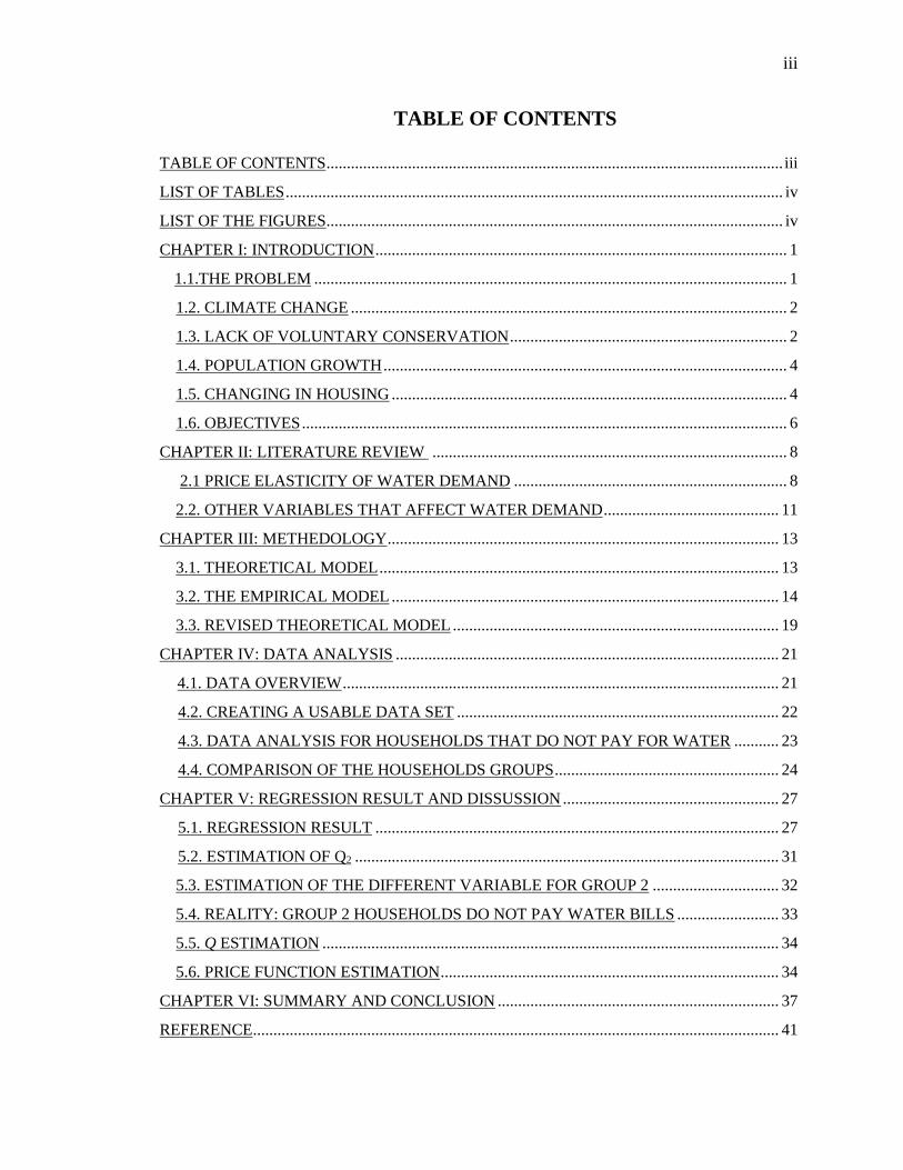
Results show that increasing the marginal price of water decreases water

consumption by 8%. Since the average water consumption of households that pay a bill is

10,135.23 gallons per month, if the marginal price increases by $1, then the water

consumption decreases by 779.2 gallons. Overall, a shift to complete volumetric pricing

will decrease average household water consumption by 5282.8 gallons per month at

existing water prices. Results also show measurable differences between cities. The

marginal price is negatively related to the water consumption levels and positively related

to the percentage of households with ‘free’ water.

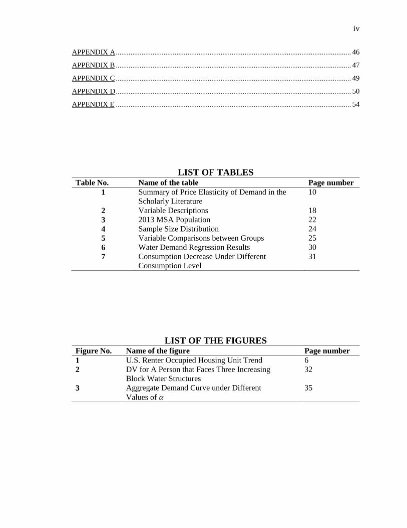
iii

TABLE OF CONTENTS

TABLE OF CONTENTS ................................................................................................................ iii

LIST OF TABLES .......................................................................................................................... iv

LIST OF THE FIGURES................................................................................................................ iv

CHAPTER I: INTRODUCTION ..................................................................................................... 1

1.1.THE PROBLEM .................................................................................................................... 1

1.2. CLIMATE CHANGE ........................................................................................................... 2

1.3. LACK OF VOLUNTARY CONSERVATION .................................................................... 2

1.4. POPULATION GROWTH ................................................................................................... 4

1.5. CHANGING IN HOUSING ................................................................................................. 4

1.6. OBJECTIVES ....................................................................................................................... 6

CHAPTER II: LITERATURE REVIEW ....................................................................................... 8

2.1 PRICE ELASTICITY OF WATER DEMAND ................................................................... 8

2.2. OTHER VARIABLES THAT AFFECT WATER DEMAND ........................................... 11

CHAPTER III: METHEDOLOGY ................................................................................................ 13

3.1. THEORETICAL MODEL .................................................................................................. 13

3.2. THE EMPIRICAL MODEL ............................................................................................... 14

3.3. REVISED THEORETICAL MODEL ................................................................................ 19

CHAPTER IV: DATA ANALYSIS .............................................................................................. 21

4.1. DATA OVERVIEW ........................................................................................................... 21

4.2. CREATING A USABLE DATA SET ............................................................................... 22

4.3. DATA ANALYSIS FOR HOUSEHOLDS THAT DO NOT PAY FOR WATER ........... 23

4.4. COMPARISON OF THE HOUSEHOLDS GROUPS ....................................................... 24

CHAPTER V: REGRESSION RESULT AND DISSUSSION ..................................................... 27

5.1. REGRESSION RESULT ................................................................................................... 27

5.2. ESTIMATION OF Q2 ........................................................................................................ 31

5.3. ESTIMATION OF THE DIFFERENT VARIABLE FOR GROUP 2 ............................... 32

5.4. REALITY: GROUP 2 HOUSEHOLDS DO NOT PAY WATER BILLS ......................... 33

5.5. Q ESTIMATION ................................................................................................................ 34

5.6. PRICE FUNCTION ESTIMATION ................................................................................... 34

CHAPTER VI: SUMMARY AND CONCLUSION ..................................................................... 37

REFERENCE ................................................................................................................................. 41

iv

APPENDIX A ................................................................................................................................ 46

APPENDIX B ................................................................................................................................ 47

APPENDIX C ................................................................................................................................ 49

APPENDIX D ................................................................................................................................ 50

APPENDIX E ................................................................................................................................ 54

LIST OF TABLES Table No. Name of the table Page number

1 Summary of Price Elasticity of Demand in the

Scholarly Literature

10

2 Variable Descriptions 18

3 2013 MSA Population 22

4

5

6

7

Sample Size Distribution

Variable Comparisons between Groups

Water Demand Regression Results

Consumption Decrease Under Different

Consumption Level

24

25

30

31

LIST OF THE FIGURES Figure No. Name of the figure Page number

1

2

3

U.S. Renter Occupied Housing Unit Trend

DV for A Person that Faces Three Increasing

Block Water Structures

Aggregate Demand Curve under Different

Values of 𝛼

6

32

35

1

CHAPTER I: INTRODUCTION

1.1 THE PROBLEM

Not so many years ago, in fact within the lifetimes of many people living in the

United States today, clean potable water was viewed as an unlimited natural resource.

Most people thought nothing of flushing five gallons or more of potable water down the

toilet and few people complained about creating artificial lakes for recreation purposes or

pumping water over mountains to irrigate deserts.1 However, the finiteness of high

quality water is becoming a greater problem in many areas, and policymakers and water

managers are concerned about ensuring a reliable supply of water for their customers

while protecting non-consumptive needs such as habitat and environmental quality.

This paper proposes a method to save one of our most important resources,

potable water, and does so using a tried and proven technology. It does this without

harming farmers, without asking plumbing companies to change their products, and

without requiring a new layer of government. Specifically, we argue that metering water

use for residential consumers significantly reduces the quantity of water used. We

develop an analytical model that highlights differences in households that pay a

volumetric fee for water versus households that pay a flat rate. We use household data to

estimate the potential reduction in water consumption form a shift to full metering.

1 There are many examples of this wasteful attitude toward water: Growing rice in California, cheap

electrical power from Hoover Dam and the Tennessee Valley Authority, water sports in Lake Mead,

bringing water to the Los Angeles Basin, and so on. In the early twentieth century, too much water was

sometimes viewed as a threat and the US Corp of Engineers job was to control this overabundance of

water, for example dredging and straightening the inland waterways. Toilets with restricted flow rates were

introduced in 1991, however existing toilet installations that flush five or even ten gallons of water per

flush are still legal to use in some parts of the United States.

2

1.2 CLIMATE CHANGE

The scarcity of adequate, clean, usable water is well documented and has

frightening consequences worldwide. Water is essential for all life and used extensively

for crop irrigation. Water is becoming a scarce resource in much of the U.S. and global

warming is expected to exacerbate that scarcity via shifts in both water demand and

supply (Karl, 2009). In the U.S., with surface temperatures rising at an average rate of

0.14oF per decade since 1901, there are ever increasing demands on limited water

supplies (EPA, 2014).

Droughts decrease water supply, draw our national consciousness to water

conservation, and cause significant economic losses. From 2012 to 2015, California had

its most severe drought since the late 1800s and farmers have had to reduce irrigated

acreage, shift from inexpensive surface water to costly and finite groundwater, and

change crops to respond to water scarcity (Wallander et al., 2015).

1.3 LACK OF VOLUNTARY CONSERVATION

Problematically, voluntary water conservation has not been effective to reduce

demand. State government officials in California proposed a 25 percent mandatory

statewide reduction in urban water use but they had only achieved a 2.8 percent reduction

by February 2015 (Nagourney & Fitzsimmons, 2015). Many newspaper reports say that

homeowners with expensive landscaping would rather pay the fines than let thousands of

dollars in residential shrubs and ornamental plants die.

3

Additionally, water shortage has become a litigious issue as individual states try

to get a larger share of the limited water supply. Recently, a lawsuit was brought by

Kansas against Nebraska over irrigation water use in the Republican River Basin. The

final settlement requires Nebraska to pay Kansas $5.5 million for estimated damages

(Knapp, 2015). Lawsuits over water use have occurred in several other interstate basins,

including the Arkansas River between Colorado and Kansas, the Pecos River between

New Mexico and Texas, and the Yellowstone River between Montana and Wyoming

(Schlager & Heikkila, 2009). One community going to court to get limited water

recourses from another community is at best a ‘quick fix’ for the winning side. This

might be important for one community, but it is not a long-term solution to fundamental

and nationwide water problems.

There is virtually universal agreement that water shortages are important

worldwide, and in the face of this urgent problem, many US communities are searching

for ways to increase available water or to increase the efficient use of this scarce

resource. Not only is water essential to life but water availability and usage are closely

related to economic growth through what has been called the “energy-water-food nexus,”

even though water is a local resource (EPA, 2013). Perhaps the first and most critical

problem for US communities is facing the potential economic losses related to water

shortage. In California alone, the net water shortage in 2014 is 1.5 million acre-feet and

the economic cost due to the drought in 2014 was estimated at $2.2 billion and there were

a total of 17,100 jobs lost (Howitt et al., 2014).

4

1.4 POPULATION GROWTH

Fifty-one percent of Americans count on ground water for their water usage

(EPA, 2008) but available groundwater has been facing continual depletion. During the

period 1900 to 2008, the volume of groundwater stored in US aquifers decreased by

about 1000 km3. The average depletion rate increased from 8.0 km3/year from 1900 until

2000, and increased to 23.9 km3/year since then (Konikow, 2015).

As population grows, more water will be demanded. The U.S. Census’s prediction

is that total U.S. population growth will increase by 98.1 million between 2014 and 2060.

The native population is expected to increase by 62 million while the foreign-born

population is projected to increase by 36 million (Colby & Ortman, 2015). With the

average person using between 80 to 120 gallons of water at home per day, future

generations will put additional pressure on the available water resources (USGS, 2016).

Most people understand that the US must find ways to use water more efficiently or face

serious consequences from inaction.

1.5 CHANGING IN HOUSING

There are increasing numbers of households living in rental properties and this is

the critical problem whose solution is discussed in this paper. In the national summary

table from 2013 American Housing Survey, 40.2 million households live in rental

properties and about 73 percent (calculated by author) of them do not pay for their water

separately. On the other hand, there are 75.7 million households that own the property

5

they live in and there are still about 30 percent that do not pay for their water separately

(AHS, 2013).2

For the households that do not pay for water separately, it is incorrect to say that

they do not pay for water. Generally, they pay a lump-sum payment that includes water in

their monthly housing payment. Therefore, they do not pay the marginal costs of water

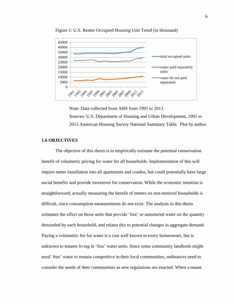
and the prices do not affect their consumption behavior. Figure 1 is the trend for U.S.

renter occupied housing unit from 1991 to 2013. Rental occupied households have

increased from 33.3 million in 1991 to 40.2 million in 2013 which was an increase of 6.9

million additional units. There was not a large increase from 1991 to 2007, but there was

a huge increase during the period 2008 to 2013 with 5.2 million added units. This was

about 75% of the total increase during 1991 to 2013. One explanation for this increase is

that millions of homeowners were displaced by foreclosures in the nation after 2008 and

that those homeowners were unable to buy a new home because of lower income during

the Great Recession (Fernald, 2013).

2 For example, many converted properties into townhouses and condo owners do not pay a water bill.

6

Figure 1: U.S. Renter Occupied Housing Unit Trend (in thousand)

Note: Data collected from AHS from 1991 to 2013

Sources: U.S. Department of Housing and Urban Development, 1991 to

2013 American Housing Survey National Summary Table. Plot by author.

1.6 OBJECTIVES

The objective of this thesis is to empirically estimate the potential conservation

benefit of volumetric pricing for water for all households. Implementation of this will

require meter installation into all apartments and condos, but could potentially have large

social benefits and provide incentives for conservation. While the economic intuition is

straightforward, actually measuring the benefit of meters on non-metered households is

difficult, since consumption measurements do not exist. The analysis in this thesis

estimates the effect on those units that provide ‘free’ or unmetered water on the quantity

demanded by each household, and relates this to potential changes in aggregate demand.

Paying a volumetric fee for water is a cost well known to every homeowner, but is

unknown to tenants living in ‘free’ water units. Since some community landlords might

need ‘free’ water to remain competitive in their local communities, ordinances need to

consider the needs of their communities as new regulations are enacted. When a tenant

0

5000

10000

15000

20000

25000

30000

35000

40000

45000

total occupied units

water paid separately

units

water do not paid

separately

7

has ‘free’ water in their rental contract, the tenant is exempt from the obligations known

by every homeowner: there is no incentive for tenants to save water or to use water

efficiently since water prices do not affect their behavior or their pocketbook.

The situation with a zero marginal cost for water is unusual, and, ‘free’ water is

unlike the normal and ordinary expected daily costs of one’s life. If one is in a high risk

profession, for example if one is a professional deep sea diver, then one expects to pay

higher than normal life insurance premiums. A fast and reckless driver with many tickets

and accidents pays a higher rate for car insurance than a driver with no citations. In other

areas of life, one expects to pay for what one gets. If a person wants to eat gourmet food,

then that person must pay a higher price than a person who lives on macaroni and cheese.

If one wears only designer outfits, then one pays higher than average prices for clothing.

The same intuition applies to homeowners and renters who pay a volumetric fee

for water consumption. A homeowner with a water meter who also has a swimming pool

and has expensive landscaping expects to pay more for water usage and accepts the cost.

On the other hand, if one lives in a ‘free’ water apartment, one does not need to care

about economics if the toilet runs night and day. One need not care about water if one

takes hour long showers. It is a serious waste of resources if there is a leaking faucet, or if

a person wastes water in any of dozens of possible ways, but there is never an economic

cost. In fact, one might believe one has a right to waste water because one has contracted

for a fixed price for a unit with unlimited water. There are no additional costs to the

household for uneconomic, poor ecologically wasteful behaviors. This is the problem.

8

CHAPTER II: LITERATURE REVIEW

This section describes previous research that analyzes the difference between

households with separate water meters with water bills and properties that have water

included in the monthly payment. There are hundreds of articles about residential water

demand analysis, but most focus on the demands and supply of single-family homes.

Only a very few studies are concerned with an analysis of 'free’ water (Goodman, 1999;

Agthe & Billings, 2002; Wentz et al., 2014; Gordon, 1999; Mayer et al., 2004). Research

from Goodman and Gordon is now over a decade old and as people have become more

aware of water scarcity and the increased pressures caused by global warming. It is time

to take a fresh look at new options for water conservation.

2.1 PRICE ELASTICITY OF WATER DEMAND

Many papers have estimated residential water demand, specifically focusing on

the price elasticity of demand. Having an accurate measure of the price elasticity of

residential water demand is critical for regulators who need to know the impact of price

changes on the quantity demanded (Olmstead, Hanemann & Stavins, 2005). The price

elasticity of demand measures the percentage changes in quantity consumed for a one

percent change in marginal price. For normal economic goods, the price elasticity of

demand is negative, which means that water consumption decreases when water price

increases. The larger the absolute value of the price elasticity, the greater the potential to

use price as a tool to conserve water resources. The literature shows a wide range of

estimates of the price elasticity for residential water demand. Espey et al. (1997)

conducted a meta-analysis based on a review of 24 journal articles published between

9

1976 and 1993 and found that increasing block rate areas have significantly more elastic

demand than others, implying that the pricing structure plays an important role in

influencing how household respond to price change.

Research conducted in Tucson, Arizona, found that in apartment complexes, the

price of water was significantly and negatively connected to the water consumption in

winter (with coefficient -1923.17 gallon2/$) and in summer (with coefficient -2160.93

gallon2/$) under linear model3. Also, the age of the apartment building (with coefficient

34.34 gallon/year in winter and 42.53 gallon/year in summer) was significantly positive

as related to apartment complex water use (Agthe & Billings, 2002).4

Not surprisingly, other research has shown that having a water meter increases the

demand elasticity. Asci and Borisova (2014) find that the price elasticity for residents

using a communal water meter, where the tenants do not pay for water directly, range

from 0 (statistically insignificant) in an instrumental variable model to -0.063 and -0.051

in 2SLS and 3SLS models. On the other hand, the price elasticity of households using a

separate water meter ranges from -0.24 to -0.31. Other work found that adding meters

(i.e., “sub metering”) to properties that provide ‘free’ water significantly reduces water

consumption (11% - 26%) from 5.55 to 17.5 kgal per unit per year or 15.2 to 47.94

gallons per unit per day (Mayer et al., 2004). A country wide study (Grafton et al., 2009)

that contain 10 OECD countries (Australia, Canada, Czech Republic, France, Italy,

Korea, Mexico, Netherlands, Norway and Sweden) found that, on average, households

that have no volumetric charge consume more water when compared to those who pay

volumetrically and high-income households are less price elastic than middle and lower

3 Coefficients are converted from cubic meter to gallon. 4 Coefficients are converted from cubic meter to gallon.

10

income households. In other words, the expected happens: When one pays for water

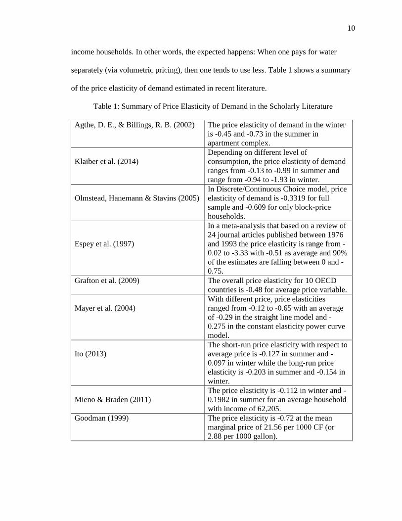
separately (via volumetric pricing), then one tends to use less. Table 1 shows a summary

of the price elasticity of demand estimated in recent literature.

Table 1: Summary of Price Elasticity of Demand in the Scholarly Literature

Agthe, D. E., & Billings, R. B. (2002) The price elasticity of demand in the winter

is -0.45 and -0.73 in the summer in

apartment complex.

Klaiber et al. (2014)

Depending on different level of

consumption, the price elasticity of demand

ranges from -0.13 to -0.99 in summer and

range from -0.94 to -1.93 in winter.

Olmstead, Hanemann & Stavins (2005)

In Discrete/Continuous Choice model, price

elasticity of demand is -0.3319 for full

sample and -0.609 for only block-price

households.

Espey et al. (1997)

In a meta-analysis that based on a review of

24 journal articles published between 1976

and 1993 the price elasticity is range from -

0.02 to -3.33 with -0.51 as average and 90%

of the estimates are falling between 0 and -

0.75.

Grafton et al. (2009)

The overall price elasticity for 10 OECD

countries is -0.48 for average price variable.

Mayer et al. (2004)

With different price, price elasticities

ranged from -0.12 to -0.65 with an average

of -0.29 in the straight line model and -

0.275 in the constant elasticity power curve

model.

Ito (2013)

The short-run price elasticity with respect to

average price is -0.127 in summer and -

0.097 in winter while the long-run price

elasticity is -0.203 in summer and -0.154 in

winter.

Mieno & Braden (2011)

The price elasticity is -0.112 in winter and -

0.1982 in summer for an average household

with income of 62,205.

Goodman (1999) The price elasticity is -0.72 at the mean

marginal price of 21.56 per 1000 CF (or

2.88 per 1000 gallon).

11

2.2 OTHER VARIABLES THAT AFFECT WATER DEMAND

Other studies have investigated how variables other than the marginal price affect

water demand. Some of these variables are about information, while others are about the

rate structure. Borisova and Useche (2013) find that extension workshops that focus on

residential water conservation effectively reduce water used in irrigation but the effect is

only temporary.

Other research has shown that the entire rate structure (not just the marginal price)

affects water consumption. In empirical studies of residential water demand, the marginal

price is commonly given as a variable price. In the residential electricity demand analysis

with increase block rate, Taylor (1975) suggests that if the average and the marginal price

are positively correlated, an upward bias might occur in the estimation of price elasticity

if only one is included as an explanatory variable. Nordin (1976) suggests the use of

difference variables (also referred to as "rate structure premium") that are defined as "a

lump-sum payment that the customer must pay before being allowed to buy as many units

as he wants at the marginal price" to correct the upward bias. Because of the similarity

between residential water demand and residential electricity demand, the difference

variable is used in our analysis. When households face nonlinear water rate structures,

they react to the average price instead of the marginal price. Also, when both the

marginal and average price are included in the estimation of price elasticity, the marginal

price (also for the expected marginal price) has nearly zero effect on water consumption,

but the average price has a significant effect on water consumption (Ito, 2013). The

difference variable is correlated with the average price, since a larger value implies a

lower average price.

12

Households are also more sensitive to price change in periods of drought and use

restrictions and landscaping programs that proved effective in reducing water usage

during a drought (Corral, Fisher, Hatch, 1999). Information on price and consumption

also affects household water demand. When the bill shows a marginal price, the price

elasticity increases from -0.36 (without price information) to -0.51 (Gaudin, 2006).

We can summarize this section as follows: When households receive a water bill,

then they behave similarly to single-family homeowners and like households behave

when they receive other utility bills such as electricity. When one receives a bill, then one

pays extra attention to the costs that created that bill. When one does not receive a bill,

one is able to disregard utility usage and the actual costs of that utility. Conservation is

normal when one receives a reminder when that reminder takes the form of a utility bill.

One would expect nothing less.

13

CHAPTER III: METHODOLOGY

3.1 THEORETICAL MEDEL

The total households for residential water can be divided into two groups:

households that pay water bills (Group 1) and households that do not pay water bills

(Group 2). We assumed there are 𝑛1 households in Group 1 and 𝑛2 households in Group

2, thus the total population is 𝑛1 + 𝑛2. Also 𝑄1 and 𝑄2 are representative household

residential water demand for Group 1 and Group 2 while 𝑄 is the representative

household demand for total population, and 𝑄 is simply a weighted average of the two

quantities demand. Therefore, the aggregate demand is:

(𝑛1 + 𝑛2) ∗ 𝑄 = 𝑛1 ∗ 𝑄1 + 𝑛2 ∗ 𝑄2 ⋯ ⋯ ⋯ ⋯ ⋯ ⋯ ⋯ ⋯ ⋯ ⋯ ⋯ ⋯ ⋯ ⋯ ⋯ ⋯ (1)

To normalize population to 1, we divided 𝑛1 + 𝑛2 in both sides and get

𝑄 = 𝑛1

𝑛1+𝑛2∗ 𝑄1 +

𝑛2

𝑛1+𝑛2∗ 𝑄2 ⋯ ⋯ ⋯ ⋯ ⋯ ⋯ ⋯ ⋯ ⋯ ⋯ ⋯ ⋯ ⋯ ⋯ ⋯ ⋯ ⋯ ⋯ (2)

where the quantity 𝑛1

𝑛1+𝑛2 is the percentage of households that pay for water and

𝑛2

𝑛1+𝑛2 is

the percentage of households that do not pay for water. We use α to represent 𝑛2

𝑛1+𝑛2 , thus

𝑛1

𝑛1+𝑛2= 1 − 𝛼.

Therefore, from equation (2) we can get

𝑄 = (1 − 𝛼) ∗ 𝑄1 + 𝛼 ∗ 𝑄2 ⋯ ⋯ ⋯ ⋯ ⋯ ⋯ ⋯ ⋯ ⋯ ⋯ ⋯ ⋯ ⋯ ⋯ ⋯ ⋯ ⋯ ⋯ ⋯ (3)

The demand function for a member of group i (i = 1, 2) is given by

𝑄𝑖 = 𝑓(𝐼, 𝑀𝑃𝑖 , 𝐷𝑉, 𝐶, 𝐶𝑙) ⋯ ⋯ ⋯ ⋯ ⋯ ⋯ ⋯ ⋯ ⋯ ⋯ ⋯ ⋯ ⋯ ⋯ ⋯ ⋯ ⋯ ⋯ ⋯ ⋯ (4)

where, MP is the marginal price of last block that household consumed (note that MP2 is

zero); DV is the difference between what household should pay if all water units were

14

charged at last block marginal price and what the household actually paid; I is the

household income; C is a vector of household characteristics; and Cl is a vector of

climate variables.

In empirical work, we normally can only observed demand 𝑄1 for households that

pay for water. We can only predict 𝑄2 from an estimate of how various explanatory

variables affect 𝑄1 when the marginal price is zero. While the parameter α does not have

a direct effect on either 𝑄1 or 𝑄2, it will affect the aggregate demand 𝑄, which is a

weighted average of the two quantities.

3.2 THE EMPIRICAL MODEL

As Olmstead et al. (2005), Mieno & Braden (2011), Ito (2013) do, we use log-log

model to estimate lnQ1 and the regression equation is:

ln(𝑄1) = 𝛽0 + 𝛽1𝐷𝐼𝑆𝐻 + 𝛽2𝑀𝐸𝑇𝑅𝑂 + 𝛽3𝑇𝐸𝑁𝑈𝑅𝐸 + 𝛽4𝑊𝐴𝑆𝐻 + 𝛽5𝐵𝐴𝑇𝐻𝑆

+ 𝛽6𝐻𝐴𝐿𝐹𝐵 + 𝛽7𝑙𝑛(𝐺𝑅𝐴𝐷𝐿𝐸𝑉𝐸𝐿) + 𝛽8𝑙𝑛(𝐻𝐻𝐴𝐺𝐸) + 𝛽9𝑙𝑛(𝑃𝐸𝑅)

+ 𝛽10𝑙𝑛(𝑌𝐸𝐴𝑅) + 𝛽11𝑙𝑛(𝐼𝑁𝐶𝑂𝑀𝐸) + 𝛽12𝑀𝑃 + 𝛽13𝐷𝑉

+ 𝛽14𝑙𝑛(𝑀𝑜𝑛𝑡ℎ𝑙𝑦𝑇𝐸𝑀) + 𝛽15𝑙𝑛(𝑀𝑜𝑛𝑡ℎ𝑙𝑦𝑅𝐴𝐼𝑁) + 𝜀

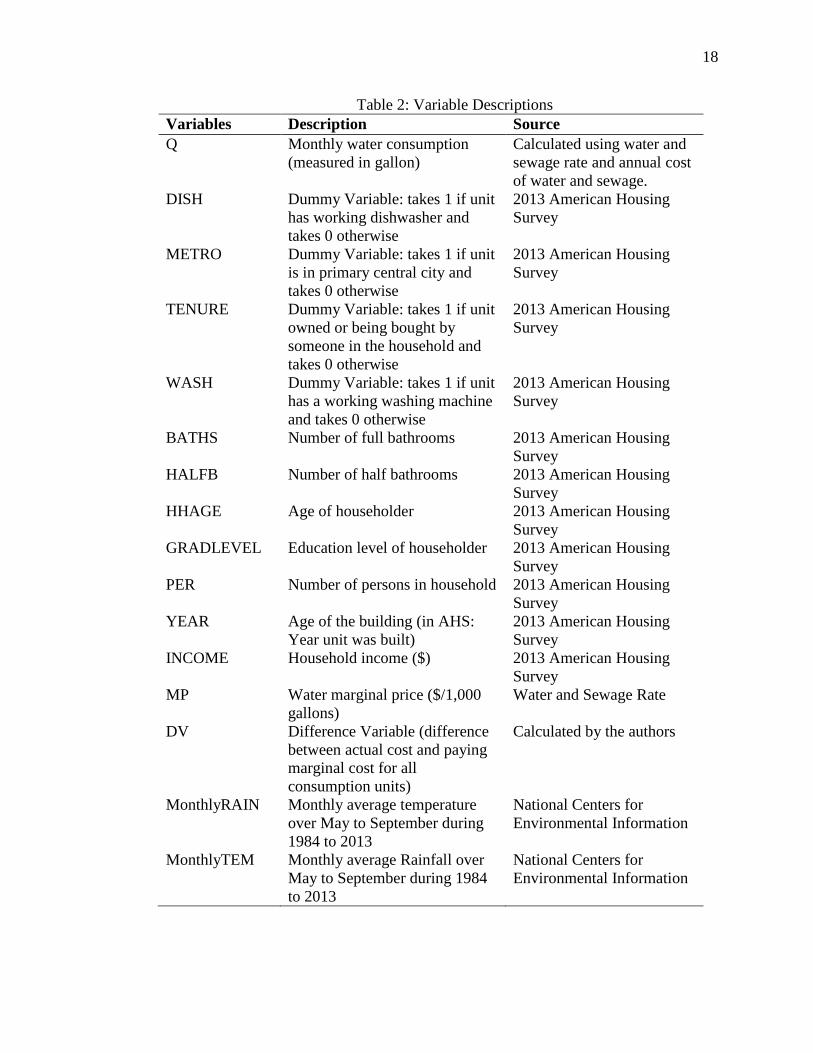
Table 2 shows the detail description for each variable in the regression equation. The

number of full bathrooms (BATHS) and half bathrooms (HALFB) are used in our

analysis. We expect the coefficients to be positive for both BATHS and HALFB since in

general, whatever valves were installed in the full baths should be the same as those in

the half baths. Properties may have been remodel or updated, but this should not affect

our methodology. It is possible that the number of bathrooms in the property could

15

change behavior. For example, having more bathrooms in a house or apartment could

encourage residents to use more water, such as by taking longer showers.

Age of the building (YEAR) could affect water consumption since older buildings

might be more likely to have fewer water saving features and less water efficient devices

(faucets, toilets, showers.). Also, the valves in older buildings may not be working

properly (e.g., leaking faucets, for example, or toilets that continue to fill after flushing).

We include 4 dummy variables that related to household characteristic. Having a

working dishwasher (DISH) and washing machine (WASH) are expected to have a

positive effect on water consumption. Even though households need to clean dishes

whether they owned dishwasher or not, the dishwasher could potentially use more water

because the dishwasher will potentially take a longer time to clean dishes.5

On the other hand, the clothes washing machine has a different impact on water

consumption. If the household does not have a working washing machine, these people

would need to wash their clothes somewhere else. This means the water usage on

washing clothes would not be in these household’s water bills. Instead they would have

to pay to clean their clothes in another location, for example ‘do it yourself’ laundry or at

a professional cleaner. Clearly the in-home water use will be higher when there is a

washing machine in the residence. However, we expect that there is a net increase in

water consumption relative to home and laundromat use because of the convenience of

having a washing machine readily available.

We use METRO dummy variable to indicate whether a household is in downtown

area. There is different life style between downtown and suburban of a metropolitan area.

5 Generally, dishwashers wash dishes twice whereas hand washing would occur one time only. Also, many

dishwashers have a ‘one hour’ cycle. In both cases, mechanical dishwashing uses more water.

16

Dummy variable (TENURE) is used for whether the household owns the house or

rent the house. We want to estimate whether there is different effect on water usage

between the house that is rented by the household and that owned by the household.

The age (HHAGE) of the head of the household, that person’s education level

(HHGRAD), and the number of persons in the household (PER) are used in our analysis.

Climate variables are also commonly used on residential water demand analysis

(Kenney et al., 2008; Klaiber et al., 2014; Asci & Borisova, 2014). In our regression

analysis, we include average May-September temperature and rainfall the 1984 to 2013.

We do not include winter climate variables in our analysis since households usually do

not consume water for outdoor purposes during winter. We did not adjust the relevant

season for southern climates (e.g., Miami) relative to northern cities (e.g. Boston), though

the region could affect the relevant season.

On a problem as complex as this, many other considerations could have been

included, for example the socioeconomic conditions of the community and variations in

building codes from one community to another. A region that has a strong ‘green

conscious’ population, a community that might be more sensitive to natural resource

issues, might behave differently from a community without this commitment.

However, we are limited in the data that we have available for the analysis. We do

believe that the balanced distribution of our sample communities keeps our analysis

relevant to a large range of cities and conditions. We have Northern, Southern,

Midwestern, and Eastern communities, we have communities from the largest population

centers down to communities of under one million people, we have communities that

have varied sources for their water, and both communities that have current water

17

shortages and communities that have none. The variety of our sample locations is an

important strength of the analysis.

18

Table 2: Variable Descriptions

Variables Description Source

Q Monthly water consumption

(measured in gallon)

Calculated using water and

sewage rate and annual cost

of water and sewage.

DISH Dummy Variable: takes 1 if unit

has working dishwasher and

takes 0 otherwise

2013 American Housing

Survey

METRO Dummy Variable: takes 1 if unit

is in primary central city and

takes 0 otherwise

2013 American Housing

Survey

TENURE Dummy Variable: takes 1 if unit

owned or being bought by

someone in the household and

takes 0 otherwise

2013 American Housing

Survey

WASH Dummy Variable: takes 1 if unit

has a working washing machine

and takes 0 otherwise

2013 American Housing

Survey

BATHS Number of full bathrooms 2013 American Housing

Survey

HALFB Number of half bathrooms 2013 American Housing

Survey

HHAGE Age of householder 2013 American Housing

Survey

GRADLEVEL Education level of householder 2013 American Housing

Survey

PER Number of persons in household 2013 American Housing

Survey

YEAR Age of the building (in AHS:

Year unit was built)

2013 American Housing

Survey

INCOME Household income ($) 2013 American Housing

Survey

MP Water marginal price ($/1,000

gallons)

Water and Sewage Rate

DV Difference Variable (difference

between actual cost and paying

marginal cost for all

consumption units)

Calculated by the authors

MonthlyRAIN Monthly average temperature

over May to September during

1984 to 2013

National Centers for

Environmental Information

MonthlyTEM Monthly average Rainfall over

May to September during 1984

to 2013

National Centers for

Environmental Information

19

3.3 REVISED THEORETICAL MODEL

For consistency with the log-log empirical model we need to revise the analytical

model. We have values of ln (𝑄1) from the household survey. We do not have actual

values of 𝑄2 due to a lack of meters. We calculate values for ln (𝑄2)̂ based on the

regression coefficients from the ln (𝑄1) demand estimation and characteristics of the

households in Group 2. Then,

𝑄 = 𝛼 ∗ 𝐸𝑋𝑃[ln(𝑄2)̂ ] + (1 – 𝛼) ∗ 𝐸𝑋𝑃[ln (𝑄1)] ⋯ ⋯ ⋯ ⋯ ⋯ ⋯ ⋯ ⋯ ⋯ ⋯ ⋯ ⋯ ⋯ (5)

Set 𝑙𝑛(𝑄1) = 𝑋1 + 𝛽12 ∗ 𝑝 and 𝑙𝑛𝑄2̂ = 𝑋2

Then we can get

𝐸𝑋𝑃(𝑋1) =𝑄1

𝐸𝑋𝑃(𝛽12 ∗ 𝑝)

and

𝐸𝑋𝑃(𝑋2) = 𝐸𝑋𝑃(𝑙𝑛𝑄2)̂

where 𝛽12 is the price coefficient of Group 1 demand; 𝑝 is the marginal price; 𝑋1

and 𝑋2 are the aggregate terms of all other variables except for the marginal price

variable for 𝑙𝑛 (𝑄1) and 𝑙𝑛𝑄2̂ respectively. Then, we can get

𝑄 = 𝛼 ∗ 𝐸𝑋𝑃(𝑋2) + (1 – 𝛼) ∗ 𝐸𝑋𝑃(𝑋1 + 𝛽12 ∗ 𝑝)

= 𝛼 ∗ 𝐸𝑋𝑃(𝑋2) + (1 – 𝛼) ∗ 𝐸𝑋𝑃(𝑋1) ∗ 𝐸𝑋𝑃(𝛽12 ∗ 𝑝) ⋯ ⋯ ⋯ ⋯ ⋯ ⋯ ⋯ ⋯ ⋯ ⋯ ⋯ (6)

Thus,

𝑄 − 𝛼 ∗ 𝐸𝑋𝑃(𝑋2)

(1 – 𝛼) ∗ 𝐸𝑋𝑃(𝑋1)= 𝐸𝑋𝑃( 𝛽12 ∗ 𝑝) ⋯ ⋯ ⋯ ⋯ ⋯ ⋯ ⋯ ⋯ ⋯ ⋯ ⋯ ⋯ ⋯ ⋯ ⋯ ⋯ ⋯ ⋯ (7)

Thus,

𝑝 =ln [

𝑄 − 𝛼 ∗ 𝐸𝑋𝑃(𝑋2)(1 – 𝛼) ∗ 𝐸𝑋𝑃(𝑋1)

]

𝛽12⋯ ⋯ ⋯ ⋯ ⋯ ⋯ ⋯ ⋯ ⋯ ⋯ ⋯ ⋯ ⋯ ⋯ ⋯ ⋯ ⋯ ⋯ ⋯ ⋯ ⋯ (8)

20

where 𝑄( 𝛼 ∗ 𝐸𝑋𝑃(𝑋2), 𝐸𝑋𝑃(𝑋2)); α is the percentage of households that do not

pay their water bill and 𝛼( 0, 1); 𝛽12 is the price coefficient of Group 1 demand.

21

CHAPTER IV: DATA ANALYSIS

4.1 DATA OVERVIEW

In this section we discuss the data that we use for the empirical analysis. The

majority of variables are from the American Housing Survey (AHS) 2013 Metropolitan

Public Use File micro household data (AHS-PUF, 2013). The American Housing Survey

is conducted biennially between May and September in odd-numbered years and the

purpose of the survey is to provide a current and continuous series of data on selected

housing and demographic characteristics. There are approximately 84,400 housing units

in the national sample and “Each housing unit in the AHS national sample is weighted

and represents about 2,000 housing units in the United States” (AHS, 2014).

Among the metropolitan areas included in the AHS, we selected populations from

within the top 50 MSA populations, ones that are generally representative of the

contiguous 48 states. We want the sample to reflect a variety of water demands and

supply conditions, so we include communities that vary not only in size and location, but

in the sources they use to get their water. We included communities that use both surface

water and underground aquifers.

For a balanced analysis, we also need our sample to come from the various

geographic and climate conditions of the US. We choose to select neither the largest nor

the smallest communities in the MSA populations but populations that are representative

of the whole country. Table 3 lists the metropolitan areas used in our analysis and the

population of each area. We choose these eight MSA from AHS 2013 Metropolitan

Statistical Areas.

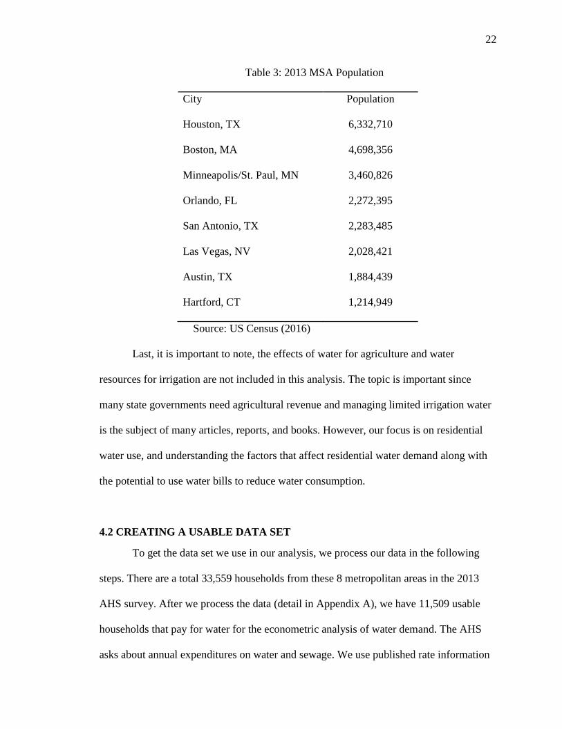
22

Table 3: 2013 MSA Population

City Population

Houston, TX 6,332,710

Boston, MA 4,698,356

Minneapolis/St. Paul, MN 3,460,826

Orlando, FL 2,272,395

San Antonio, TX 2,283,485

Las Vegas, NV 2,028,421

Austin, TX 1,884,439

Hartford, CT 1,214,949

Source: US Census (2016)

Last, it is important to note, the effects of water for agriculture and water

resources for irrigation are not included in this analysis. The topic is important since

many state governments need agricultural revenue and managing limited irrigation water

is the subject of many articles, reports, and books. However, our focus is on residential

water use, and understanding the factors that affect residential water demand along with

the potential to use water bills to reduce water consumption.

4.2 CREATING A USABLE DATA SET

To get the data set we use in our analysis, we process our data in the following

steps. There are a total 33,559 households from these 8 metropolitan areas in the 2013

AHS survey. After we process the data (detail in Appendix A), we have 11,509 usable

households that pay for water for the econometric analysis of water demand. The AHS

asks about annual expenditures on water and sewage. We use published rate information

23

from each MSA to derive the household water quantity consumed (details on this process

are in Appendix B). Table 4 shows the sample size of households that pay for water in

each city.

Among these 8 MSA are three forms of rate structure: two communities with

uniform rate structure (Hartford, Minneapolis); three communities with increasing block

rate structure (Austin (total 5 blocks), Boston (total 6 blocks), Las Vegas (total 4 blocks);

and one community with decreasing block rate structure (Houston (total 8 blocks with 3

decreasing blocks and 5 increasing blocks)), Orlando (total 5 blocks), San Antonio (total

4 blocks). We calculate marginal price and different variable for each household and the

detail is in Appendix C. The rate structure is in Appendix D.

4.3 DATA ANALYSIS FOR HOUSEHOLDS THAT DO NOT PAY FOR WATER

There are a total of 18,890 households that answer -6 (Not Applicable) for the

annual water and sewage cost (AMTW) and we assume these households do not pay

separate water bills. We infer the quantity of water consumed by each of these

households based on its actual characteristics and the estimated regression coefficients

for Group 1. Since the household characteristics provide the link to estimate consumption

for unmetered households, it is critical that we have accurate information about those

characteristics. Thus, we exclude households that are missing more than one of the

explanatory variables included in the demand estimation, or those that report no income

or negative income. Our final usable dataset has 9,185 households that do not pay for

water (see in Appendix E). The distribution of these households by MSA is in Table 4.

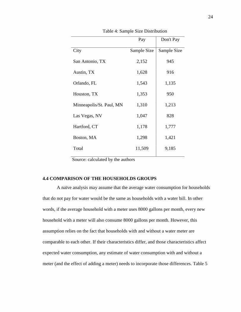
24

Table 4: Sample Size Distribution

Pay Don't Pay

City Sample Size Sample Size

San Antonio, TX 2,152 945

Austin, TX 1,628 916

Orlando, FL 1,543 1,135

Houston, TX 1,353 950

Minneapolis/St. Paul, MN 1,310 1,213

Las Vegas, NV 1,047 828

Hartford, CT 1,178 1,777

Boston, MA 1,298 1,421

Total 11,509 9,185

Source: calculated by the authors

4.4 COMPARISON OF THE HOUSEHOLDS GROUPS

A naïve analysis may assume that the average water consumption for households

that do not pay for water would be the same as households with a water bill. In other

words, if the average household with a meter uses 8000 gallons per month, every new

household with a meter will also consume 8000 gallons per month. However, this

assumption relies on the fact that households with and without a water meter are

comparable to each other. If their characteristics differ, and those characteristics affect

expected water consumption, any estimate of water consumption with and without a

meter (and the effect of adding a meter) needs to incorporate those differences. Table 5

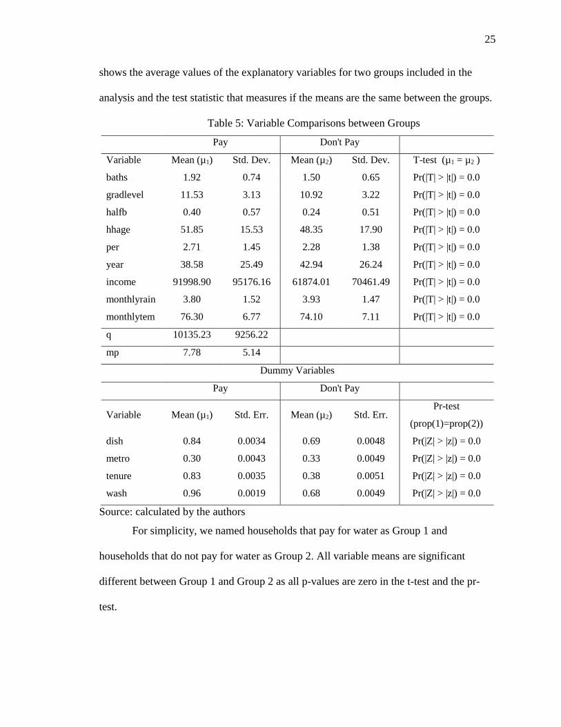
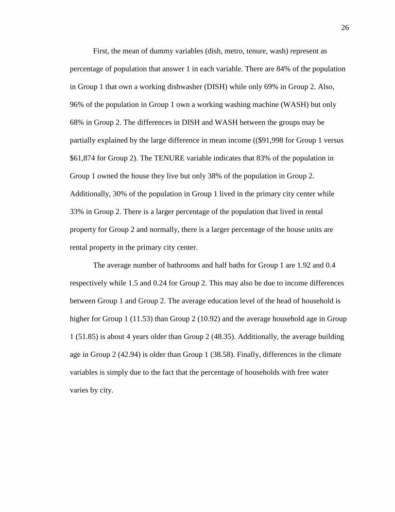
25

shows the average values of the explanatory variables for two groups included in the

analysis and the test statistic that measures if the means are the same between the groups.

Table 5: Variable Comparisons between Groups

Pay Don't Pay

Variable Mean (µ1) Std. Dev. Mean (µ2) Std. Dev. T-test (µ1 = µ2 )

baths 1.92 0.74 1.50 0.65 Pr(|T| > |t|) = 0.0

gradlevel 11.53 3.13 10.92 3.22 Pr(|T| > |t|) = 0.0

halfb 0.40 0.57 0.24 0.51 Pr(|T| > |t|) = 0.0

hhage 51.85 15.53 48.35 17.90 Pr(|T| > |t|) = 0.0

per 2.71 1.45 2.28 1.38 Pr(|T| > |t|) = 0.0

year 38.58 25.49 42.94 26.24 Pr(|T| > |t|) = 0.0

income 91998.90 95176.16 61874.01 70461.49 Pr(|T| > |t|) = 0.0

monthlyrain 3.80 1.52 3.93 1.47 Pr(|T| > |t|) = 0.0

monthlytem 76.30 6.77 74.10 7.11 Pr(|T| > |t|) = 0.0

q 10135.23 9256.22

mp 7.78 5.14

Dummy Variables

Pay Don't Pay

Variable Mean (µ1) Std. Err. Mean (µ2) Std. Err. Pr-test

(prop(1)=prop(2))

dish 0.84 0.0034 0.69 0.0048 Pr(|Z| > |z|) = 0.0

metro 0.30 0.0043 0.33 0.0049 Pr(|Z| > |z|) = 0.0

tenure 0.83 0.0035 0.38 0.0051 Pr(|Z| > |z|) = 0.0

wash 0.96 0.0019 0.68 0.0049 Pr(|Z| > |z|) = 0.0

Source: calculated by the authors

For simplicity, we named households that pay for water as Group 1 and

households that do not pay for water as Group 2. All variable means are significant

different between Group 1 and Group 2 as all p-values are zero in the t-test and the pr-

test.

26

First, the mean of dummy variables (dish, metro, tenure, wash) represent as

percentage of population that answer 1 in each variable. There are 84% of the population

in Group 1 that own a working dishwasher (DISH) while only 69% in Group 2. Also,

96% of the population in Group 1 own a working washing machine (WASH) but only

68% in Group 2. The differences in DISH and WASH between the groups may be

partially explained by the large difference in mean income (($91,998 for Group 1 versus

$61,874 for Group 2). The TENURE variable indicates that 83% of the population in

Group 1 owned the house they live but only 38% of the population in Group 2.

Additionally, 30% of the population in Group 1 lived in the primary city center while

33% in Group 2. There is a larger percentage of the population that lived in rental

property for Group 2 and normally, there is a larger percentage of the house units are

rental property in the primary city center.

The average number of bathrooms and half baths for Group 1 are 1.92 and 0.4

respectively while 1.5 and 0.24 for Group 2. This may also be due to income differences

between Group 1 and Group 2. The average education level of the head of household is

higher for Group 1 (11.53) than Group 2 (10.92) and the average household age in Group

1 (51.85) is about 4 years older than Group 2 (48.35). Additionally, the average building

age in Group 2 (42.94) is older than Group 1 (38.58). Finally, differences in the climate

variables is simply due to the fact that the percentage of households with free water

varies by city.

27

CHAPTER V: REGRESSION RESULTS AND DISCUSSION

5.1 REGRESSION RESULT

The regression result in Table 6 is for estimating lnQ1. The standard error in the

parenthesis is the heteroskedastic robust standard error. The heteroskedasticity test shows

that the heteroskedasticity is present in our analysis, thus we adjust this problem by using

robust standard errors.

Most of the coefficients in the regression result were expected except for DISH

and METRO. DISH has negative coefficient and METRO has positive coefficient but

both are statistically insignificant. This makes sense, because having a working

dishwasher does not mean that the household will use it all the time and the household

might wash their dishes even without owning a dishwasher. Also, households living in

the primary city center should not use more water compared to the households that live

outside the city since households lived in the primary city center are most likely to live in

rental units.

The coefficient for TENURE is positive and statistically significant which means

that households would consume more water when they owned the property in which they

live. Number of bathroom is positive and statistically significant relative to water

consumption but number of half bathroom is statistically insignificant.

The coefficients for variables with log transformed (GRADLEVEL, HHAGE,

PER, YEAR, INCOME, MONTHLYRAIN, MONTHLYTEM) measure elasticities.

Education level is statistically insignificant while the coefficient for LN(HHAGE) is

0.082 and statistically significant. This means that if head of household’s age increases 1

28

percent, then the water consumption will increase 0.082 percent. The coefficient for

LN(YEAR) shows that if the building age increases 1 percent, then the water

consumption will increase 0.053 percent.

Household size and income are positive and statistically significant related to

water consumption. A 1 percent increase in household size or income increases water

consumption by 0.226 and 0.018 percent respectively.

In this model, we did not use log transformation on marginal price (MP) and

different variable (DV) since we want to use the coefficients from Q1 to estimate Q2. As

we mentioned, the marginal price for Group 2 is zero which means that if we use log

transformation on marginal price, then LN(MP) will be infinite. Also, under the

assumption that the demand function is the same for both groups, it would be

theoretically inconsistent with the analytical framework if we use LN(MP) as explanatory

variable. This is because by using LN(MP) in the regression means that there is a

constant elasticity demand, however this is not possible for Group 2 with marginal price

equal to zero. The coefficient for MP shows that if marginal price of water increase by 1

dollar, then the water consumption will decrease about 8% when everything else stay the

same.6 Table 7 shows the reduction in water consumption under different consumption

levels when the price is increase by 1 dollar.

Monthly rainfall is negatively related to water consumption while monthly

temperature is positively related to water consumption. Households are less responsive to

6 Proof: Assume original marginal price is MP0 and household consume q1 water at this marginal price.

After the marginal price increase $1, household consume q2 water. Since everything else stay the same, we

set the sum of other variables calculation as X. Then ln(q1) = X + (-0.08) * MP0 and ln(q2) = X + (-0.08) *

(MP0+1). We can get ln(q2) + 0.08 = ln(q1) then ln(q2/q1) = -0.08. We then take exponent on both size and

get q2/q1 = 0.923.

29

monthly rainfall since 1 percent increase in rainfall only reduces water consumption by

0.031 percent. On the other hand, households are more sensitive to monthly temperature

since 1 percent increase in temperature will increase water consumption by 1.393 percent.

30

Table 6: Water Demand Regression Results (dependent variable is ln(Q1))

Variables

DISH -0.022 (0.017)

METRO -0.021* (0.012)

TENURE 0.083*** (0.016)

WASH 0.024 (0.029)

BATHS 0.077*** (0.009)

LN(GRADLEVEL) 0.014 (0.016)

HALFB 0.011 (0.011)

LN(HHAGE) 0.082*** (0.020)

LN(PER) 0.226*** (0.012)

LN(YEAR) 0.053*** (0.008)

LN(INCOME) 0.018** (0.007)

MP -0.080*** (0.001)

DV 0.019*** (0.0002)

LN(MONTHLYRAIN) -0.031*** (0.009)

LN(MONTHLYTEM) 1.393*** (0.093)

CONSTANT 1.964*** (0.4442)

R-squared 0.561

Prob > F 0.000

N 11,509

*, **, *** indicate significance level at 10 percent, 5 percent, and 1 percent respectively.

Figures in parenthesis are heteroskedastic robust standard error.

31

Table 7: Consumption Decrease after a Water Rate Change under Different Initial

Consumption Level (in gallons)

Source: calculated by the authors

5.2 ESTIMATION OF Q2

We assume that the demand functions Q1 and Q2 are identical and the only

difference is that the marginal price for Q2 is zero and the difference variable depend on

marginal price. Thus, the coefficients in Q2 are the same as Q1 and we use these

coefficients from Q1 to estimate demand function Q2, conditional on the actual household

characteristics of Group 2. For increasing block rate structures, the different variable

(DV) acts as income subsidy since the marginal price increases as households consume

Original

Consumption Level

Post Consumption Level

when Price Increases $1 Decrease in Consumption

1000 923.1 76.9

2000 1846.2 153.8

3000 2769.3 230.7

4000 3692.5 307.5

5000 4615.6 384.4

6000 5538.7 461.3

7000 6461.8 538.2

8000 7384.9 615.1

9000 8308.0 692.0

10000 9231.2 768.8

11000 10154.3 845.7

12000 11077.4 922.6

13000 12000.5 999.5

14000 12923.6 1076.4

15000 13846.7 1153.3

32

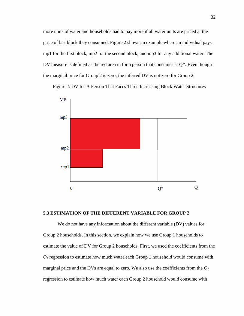
more units of water and households had to pay more if all water units are priced at the

price of last block they consumed. Figure 2 shows an example where an individual pays

mp1 for the first block, mp2 for the second block, and mp3 for any additional water. The

DV measure is defined as the red area in for a person that consumes at Q*. Even though

the marginal price for Group 2 is zero; the inferred DV is not zero for Group 2.

Figure 2: DV for A Person That Faces Three Increasing Block Water Structures

5.3 ESTIMATION OF THE DIFFERENT VARIABLE FOR GROUP 2

We do not have any information about the different variable (DV) values for

Group 2 households. In this section, we explain how we use Group 1 households to

estimate the value of DV for Group 2 households. First, we used the coefficients from the

Q1 regression to estimate how much water each Group 1 household would consume with

marginal price and the DVs are equal to zero. We also use the coefficients from the Q1

regression to estimate how much water each Group 2 household would consume with

33

marginal prices and the DV values are equal to zero. For each Group 2 household in the

sample, we match the Group 1 household with smallest consumption that is greater than

or equal to the estimate of the Group 2 household from that MSA. For each matched pair,

we used the marginal price and the DV values from the Group 1 household to replace the

marginal price and the DV values for Group 2. This process is done within each city so

that matches are as similar as possible.

After all households in Group 2 are matched and replaced with the price variables

from the households in Group 1, we have complete data for Group 2 households. Using

the coefficients from the Q1 regression, we estimate that the average monthly water

consumption for Group 2 households (conditional on Group 2 households having meters

and paying for water) is 6,118.71 gallons (110.02 gallons per day per person). The

observed average monthly water consumption for Group 1 households is 10,135.23

gallons (157.64 gallons per day per person). Thus, the average per person daily water

consumption for Group 1 households is about 47 gallons more than Group 2 when both

groups pay water bills.

5.4 REALITY: GROUP 2 HOUSEHOLDS DO NOT PAY WATER BILLS

In reality, Group 2 households do not pay water bills. This means that the

marginal price is zero; however, the DV for Group 2 households is not zero (except for

flat rate cities) because as long as households consume more than first block size, then

the DV will be positive with increasing block rates. We also know that for households in

Group 2, the actual DV will be at least as large as the estimate based on paying the water

bill (the estimation method is described in the previous section). We know households in

34

Group 2 would consume more water when the marginal price is zero which means that

the value of the DV will be larger. Thus, when Group 2 households do not pay water

bills, the value of the DV should at least be as large as when they do pay water bills. With

the marginal price equal to zero and the DV stays the same, the average monthly water

consumption for Group 2 households is 11,401.51 gallons (199.3 gallons per day per

person). Therefore, on average, each person in Group 2 will save 89.28 gallons of water

per day when Group 2 households pay water bills.

5.5 Q ESTIMATION

Last, one of our main objectives is to estimate an aggregate Q, or one that is

representative of the “average” household. While we assume that the individual

household demand does not change, the aggregate demand depends on the proportion of

households that pay for water. For water utilities, this is the most important measure since

it reflects the expected total consumption and water needs that must be provided. To

estimate Q, we need to get the value of α. There are 11,509 households in Group 1 and

9,185 households in Group 2 with total 20,694 households. Thus, α is equal to 44.4% (α

9185/20694) and 1 – α is 55.6%. We rewrite equation (3) as

𝑄 = 0.556 ∗ 𝐸𝑋𝑃(𝑙𝑛(𝑄1)) + 0.444 ∗ 𝐸𝑋𝑃((ln(𝑄2)̂ )) ⋯ ⋯ ⋯ ⋯ ⋯ ⋯ ⋯ ⋯ ⋯ ⋯ (9)

5.6 PRICE FUNCTION ESTIMATION

From the theoretical model, we know the price function is

𝑝 =ln [

𝑄 − 𝛼 ∗ 𝐸𝑋𝑃(𝑋2)(1 – 𝛼) ∗ 𝐸𝑋𝑃(𝑋1)

]

𝛽12

35

where 𝑄( 𝛼 ∗ 𝐸𝑋𝑃(𝑋2), 𝐸𝑋𝑃(𝑋2)).

From the empirical demand estimation result, we calculate that EXP(X1) equals 18284.25

gallons and EXP(X2) equals 11401.51 gallons. Also, 𝛽12 is equal to -0.08 gallon^2/$.

Then we get the price function as

𝑝 =ln [

𝑄 − 𝛼 ∗ 𝐸𝑋𝑃(𝑋2)(1 – 𝛼) ∗ 𝐸𝑋𝑃(𝑋1)

]

𝛽12=

ln [𝑄 − 𝛼 ∗ 11401.51

(1 – 𝛼) ∗ 18284.25)]

−0.08⋯ ⋯ ⋯ ⋯ ⋯ ⋯ ⋯ ⋯ ⋯ ⋯ (10)

Figure 3 shows the aggregate demand curve under different values of 𝛼.

Figure 3: Aggregate Demand Curve under Different Values of 𝛼

The α is equal to 0.444 from the empirical data. We plug in the value of α and get

the price function as

𝑝 =ln [

𝑄 − 5062.2710166.04 ]

−0.08⋯ ⋯ ⋯ ⋯ ⋯ ⋯ ⋯ ⋯ ⋯ ⋯ ⋯ ⋯ ⋯ ⋯ ⋯ ⋯ ⋯ ⋯ ⋯ ⋯ ⋯ ⋯ ⋯ ⋯ (11)

where 𝑄( 5062.27, 11401.51).

36

Then we can get

𝑑𝑝

𝑑𝑄=

1

404.98−0.08∗𝑄 ⋯ ⋯ ⋯ ⋯ ⋯ ⋯ ⋯ ⋯ ⋯ ⋯ ⋯ ⋯ ⋯ ⋯ ⋯ ⋯ ⋯ ⋯ ⋯ ⋯ (12)

As we can see, as 𝑄 gets larger, the rate of change gets smaller.

37

CHAPTER VI: SUMMARY AND CONCLUSIONS

In this thesis, we use the data from 2013 American Housing Survey Metropolitan

to estimate the potential water conservation when households pay water bills. There are

two types of households in our analysis: households that pay water bills (Group 1) and

households that do not pay water bills (Group 2). We use log-log model to estimate

Group 1 log-transformation (𝑙𝑛𝑄1) demand and then use 𝑙𝑛𝑄1 coefficient to estimate the

water consumption level for Group 1 and Group 2 households after we set the marginal

price and DV equal to zero. We use these consumption levels to match Group 2

households with Group 1 households under each MSA. For each matched pair, the

marginal price and DV for Group 2 households were replaced by the Group 1

household’s marginal price and DV. Then we estimate the consumption level for Group 2

households when they pay water bills and when they do not pay a water bills. The

difference in consumption when Group 2 households pay water bills and do not pay water

bills is the potential water conservation. The numbers show us what one might have

assumed before beginning the analysis: billing for a utility will cause some people to

restrict usage. The consumer pays closer attention to usage and monitors waste.

Our work confirms what Grafton et al. (2009) has found using data from 10

OECD countries in Asia, Latin American, and Europe. Researchers found that having

metered water makes consumers more conservative with water usage.

People realize that shortages of potable water exist today and that shortages will

only increase in the future. Solutions are critical; however, solutions do exist. For

example, in September 2015, higher efficiency water heater became mandated by law.

38

Today, toilets flush with under one and one half gallon per flush whereas older toilets

flushed with three and one half gallons per flush.

Multifamily living was common as populations moved into the cities, beginning

over a hundred and fifty years ago, when water was not viewed as a scarce natural

resource at all. In fact, water was thought of as both a problem and a solution at the same

time. Water was not scarce, so rice could be grown in deserts; dams could be built for

electric power and irrigation, and water could even be pumped over the California

foothills to a desert called the LA basin. No could see the coming problems.

Next, when there is no direct economic fee for a wasteful behavior when water is

not billed. Even people who are concerned about the environment can be wasteful when

a person does not need to pay.

It is a reasonable hypothesis that ‘free’ water households are similar to other

world populations, the same as the ordinary American homeowners, and will tend not to

behave differently about their water use unless there are mandatory restrictions or if they

are incentivized to consider conservation because of a change in water rates. As an added

benefit, remodeling and building contractors will have new work opportunities. There are

additional billing hours for licensed plumbers and the manufacturers of residential water

meters will have increased volume. These should be good for a country with eight years

of a stagnant residential construction market.

One might assume that objections could come from building owners who fear

new remodeling costs. This could be a reasonable objection until one considers the

potential benefits to our country. A review of residential water meters advertised on the

internet shows prices from about $90 to $160 per unit, depending on the features and the

39

warranty offered. Our model estimates that the average household going from non-

metered to metered water would save on average about 5,000 gallons of water per month.

With the current average marginal price of water in our Group 1 sample at $7.78 per

1,000 gallons, the water meter would be paid for in 3 to 4 months, less the cost of

installation.

Building owners know and accept that changes in plumbing and electrical codes

that are required in new construction. Existing units can and should be phased in over a

span of time. As we have seen in water restrictions in residential toilets and faucets,

existing buildings are phased in and do not cause an undue burden to owners. Only an

analysis of construction costs could answer this question and that is beyond the scope of

this paper.

Last, and perhaps most important, the measure will be popular with people who

are concerned about the diminishing availability of potable water. This should include

powerful groups like the National Resources Defense Council and those voters who

consider themselves part of the ‘green revolution’. Non metered households may worry

that their utility costs could go up, but our analysis shows that this is usually not the case.

This is not an unusual proposal. During the early 1990s, the Federal government

passed a simple law requiring toilets to flush with no more than 1.2 gallons per flush. At

that time, the average toilet flushed with 3.5 gallons of water with each flush. Both non

metered households and single family owned homes were given a discount voucher to

make the change to efficient toilets. This law saved hundreds of thousands of gallons of

clean, potable water that were being flushed down inefficient toilets. Nothing was lost.

40

Just last year, Federal regulations changed for water heaters making them more

energy efficient. Manufacturers where allowed to sell of their stocks and retailers were

given a full year to dispose of the older, less efficient models. This process is still going

on and has not disrupted the availability of water heaters and the major manufacturers

have been willing partners in the changeover. Residential faucets and showers have gone

through similar flow restrictions without problems of supply or engineering. Fortunately,

there is no major industry that could be harmed by this proposal, and like the changes in

residential flow rates, one could expect this change to mirror water flow rates changes

and be welcomed.

This is a democratic proposal. If one wishes to take hour long showers, then

nothing in this proposal takes that privilege away. The only change is that each person

must pay their fair share of the costs for their behavior; a very American point of view.

41

REFERENCE

Agthe, D. E., & Billings, R. B. (2002). Water price influence on apartment complex

water use. Journal of water resources planning and management, 128(5), 366-

369.

AHS, 2013. National Summary Tables - AHS 2013. America Housing Survey. Retrieved

March 4, 2015, from http://www.census.gov/programs-

surveys/ahs/data/2013/national-summary-report-and-tables---ahs-2013.html

AHS, 2014. About. America Housing Survey. Retrieved March 4, 2015, from

https://www.census.gov/programs-surveys/ahs/about.html

AHS-PUF, 2013. AHS 2013 Metropolitan Public Use File (PUF). America Housing

Survey. Retrieved March 4, 2015, https://www.census.gov/programs-

surveys/ahs/data/2013/ahs-2013-public-use-file--puf-/2013-ahs-metropolitan-puf-

microdata.html

Asci, S., & Borisova, T. (2014, July). The Effect of Price and Non-Price Conservation

Programs on Residential Water Demand. In The paper is presented at the 2014

AAEA Annual Meeting, Minneapolis, MN.

Borisova, T., & Useche, P. (2013). Evaluating the Performance of Non-Price Residential

Water Conservation Programs Using Quasi-Experiments. In 2013 Annual

Meeting, August 4-6, 2013, Washington, DC (No. 151223). Agricultural and

Applied Economics Association.

Colby, S. L., & Ortman, J. M. (2015). Projections of the Size and Composition of the US

Population: 2014 to 2060. US Census Bureau, Ed, 25-1143.

42

Corral, L., Fisher, A. C., & Hatch, N. W. (1999). Price and non-price influences on water

conservation: an econometric model of aggregate demand under nonlinear budget

constraint. Department of Agricultural & Resource Economics, UCB.

EPA. (2008). U.S. Environmental Protection Agency (EPA). (2008). EPA’s 2008 Report

on the Environment. National Center for Environmental Assessment, Washington,

DC.

EPA. (2014). U.S. Environmental Protection Agency. 2014. Climate change indicators in

the United States, 2014. Third edition. EPA 430-R-14-004.

www.epa.gov/climatechange/indicators.

EPA. (2013). United States. Environmental Protection Agency. (2013). The Importance

of Water to the U.S. Economy.

Espey, M., Espey, J., & Shaw, W. D. (1997). Price elasticity of residential demand for

water: a meta‐analysis. Water Resources Research, 33(6), 1369-1374.

Fernald, M. (2013). America’s rental housing: Evolving markets and needs. Cambridge,

MA: Joint Center for Housing Studies, Harvard University. Retrieved from

http://www.jchs.harvard.edu/sites/jchs.harvard.edu/files/jchs_americas_rental_ho

using_2013.pdf

Gaudin, S. (2006). Effect of price information on residential water demand. Applied

economics, 38(4), 383-393.

Goodman, J. (1999). Water Conservation from User Charges in Multi-family Rental

Housing. Washington, DC: American Real Estate and Urban Economics

Association.

43

Gordon, L. P. (1999). The influence of individual metering on water consumption in

multi-family dwellings (Master’s Thesis, Massachusetts Institute of Technology).

Grafton, R. Q., Kompas, T., To, H., & Ward, M. (2009). Residential water consumption:

a cross country analysis. Environmental Economics Research Hub Research

Report.

Howitt, R., Medellín-Azuara, J., MacEwan, D., Lund, J., & Sumner, D. (2014).

Economic analysis of the 2014 drought for California agriculture. Davis, CA:

UC–Davis Center for Watershed Sciences. Online at https://watershed. ucdavis.

edu/files/biblio/DroughtReport_23July2014_0. pdf.

Ito, K. (2013). How do consumers respond to nonlinear pricing? Evidence from

household water demand (pp. 537-563). Working Paper, Stanford University.

Karl, T. R. (2009). Global climate change impacts in the United States. Cambridge

University Press.

Kenney, D. S., Goemans, C., Klein, R., Lowrey, J., & Reidy, K. (2008). Residential water

demand management: lessons from aurora, Colorado1.

Klaiber, H. A., Smith, V. K., Kaminsky, M., & Strong, A. (2014). Measuring price

elasticities for residential water demand with limited information. Land

Economics, 90(1), 100-113.

Knapp, F. (2015, February 24). U.S. Supreme Court rules in Kansas-Nebraska fight over

Republican River. Retrieved April 23, 2015, from

http://netnebraska.org/article/news/960629/us-supreme-court-rules-kansas-

nebraska-fight-over-republican-river

44

Konikow, L. F. (2015). Long‐Term Groundwater Depletion in the United States.

Groundwater, 53(1), 2-9.

Mayer, P. W., Towler, E., DeOreo, W. B., Caldwell, E., Miller, T., Osann, E. R., ... &

Fisher, S. B. (2004). National multiple family submetering and allocation billing

program study. Aquacraft Inc., Boulder, Colo.

Mieno, T., & Braden, J. B. (2011). Residential Demand for Water in the Chicago

Metropolitan Area1.

Nagourney, A., & Fitzsimmons, E. (2015, April 7). Under New Water Rules, Beverly

Hills Must Turn Off Taps; Santa Cruz, Less So. The New York Times. Retrieved

April 24, 2015, from http://www.nytimes.com/2015/04/08/us/californias-water-

conservation-slowed-in-february.html?_r=0

Nordin, J. A. (1976). A proposed modification of Taylor's demand analysis: comment.

The Bell Journal of Economics, 719-721.

Olmstead, S., Hanemann, W. M., & Stavins, R. N. (2005). Do Consumers React to the

Shape of Supply?: Water Demand Under Heterogeneous Price Structures. John F.

Kennedy School of Government, Harvard University.

Reporter, D. M. (2012). Obama gets into the swing of things on his Martha's Vineyard

vacation... after increasing his personal debt ceiling with rare sighting of the First

Credit Card. Retrieved Jun 28, 2016, from

http://www.dailymail.co.uk/news/article-2027541/Obama-golfs-Marthas-

Vineyard-increasing-personal-debt-ceiling.html

Schlager, E., & Heikkila, T. (2009). Resolving water conflicts: A comparative analysis of

interstate river compacts. Policy Studies Journal, 37(3), 367-392.

45

Taylor, L. D. (1975). The demand for electricity: a survey. The Bell Journal of

Economics, 74-110.

Tchigriaeva, E., Lott, C., & Rollins, K. (2014). Modeling effects of multiple conservation

policy instruments and exogenous factors on urban residential water demand

through household heterogeneity. In 2014 Annual Meeting, July 27-29, 2014,

Minneapolis, Minnesota (No. 170605). Agricultural and Applied Economics

Association.

US Census, 2016. Annual Estimates of the Resident Population: April, 2010 to July 1,

2015. US Census Bureau, Population Division. Retrieved June 23, 2016, from

http://factfinder.census.gov/faces/tableservices/jsf/pages/productview.xhtml?src=

bkmk

USGS, 2016. Water Questions & Answers. How much water does the average person use

at home per day? (n.d.). Retrieved May 09, 2016, from

http://water.usgs.gov/edu/qa-home-percapita.html

Wallander, S., Aillery, M., & Schaible, G. (2015). Long-Term Response to Water

Scarcity in California. Amber Waves, 15.

Wentz, E. A., Wills, A. J., Kim, W. K., Myint, S. W., Gober, P., & Balling Jr, R. C.

(2014). Factors Influencing Water Consumption in Multifamily Housing in

Tempe, Arizona. The Professional Geographer, 66(3), 501-510.

46

APPENDIX A

PROCESSES TO GET THE USABLE DATA SET

First, we exclude households that answer in the survey that contain -6 (Not

applicable) in AMTW. Excluding these in the variables, we have remaining 14,669

households that can be used and are available for our analysis.

Second, we exclude 457 households in the METRO section that answer 2

(households live in the secondary central city) in the METRO question. We have to

exclude these households in our analysis because we want to use METRO as dummy

variable in our analysis because the dummy variable. Similarly, we exclude 382

households that answer 3 (occupied without payment of rent) in the question about

TENURE. We are left with 14,212 households.

Third, we exclude households that report AMTW>INCOME. This leaves us with

a total of 13,830 households.

There is one more set of households excluded. When the final Q (water

consumption) is negative based on the rates, then the household is excluded in the

analysis. This is explained below.

47

APPENDIX B

PROCESSES OF CALCULATE HOUSEHOLDS WATER QUANTITY

CONSUMED

First, figure the monthly water and sewage cost by dividing AMTW by 12.

Denote new monthly water and sewage cost as ME0 (monthly water expenditure).

Second, if there are monthly fixed (or service) charges, then subtract these

charges from ME0 otherwise go to step 3. Denote new monthly water and sewage cost as

ME1. In excel, use ‘IF’ function as if ME1 is positive, then equal to ME1 otherwise 0.

Denote new ME1 as ME1’.

Third, use water and sewage rate structure to calculate the total cost needed to

consume whole block size in each block. For multiple blocks cities, denote the total cost

as BC(i) (i= 1,2,3,4,…,k is the block number and k is the last block) and denote marginal

price in each block as MP(i) ($/1000 Gallon).

Fourth, subtract BC(1) from ME1’ and denote new monthly water and sewage

cost as ME2. If ME2 is positive, then Q1 is equal to first block size otherwise Q1 is equal

to ME1’*1000/MP1. Then, use ‘IF’ function as if ME2 is positive, then equal to ME2

otherwise 0. Denote new ME2 as ME2’.

Fifth, repeat step 4 for all blocks except the last block.

Sixth, since the last block don’t have block size, the quantity consumed is equal to

ME(k)’*1000/MP(k) assuming k is the last block. And for flat rate city, the household

water quantity consumed is equal to ME1’*1000/P when P is equal to the flat water rate.

Seventh, final water quantity consumed. Add up all Qi together and get the final

water consumption quantity Q.

48

Eighth, if the final Q is negative because ME0 is less than the monthly fixed (or

service) charge, then we excluded these households in our analysis.

Ninth, we excluded households that use less than 10 gallons per day per person.

49

Appendix C

PROCESSES TO CALCULATE MARGINAL PRICE AND DIFFERENT

VARIABLE

First, copy value only for all blocks water quantity consumed, then change 0 to M

since the water quantity consumed is 0 for blocks that household do not consume.

Second, in Microsoft Excel, use ‘COUNT’ function for all blocks, then the

number shows how many blocks that household consumed and denoted as NB (number

of blocks). Then, use ‘IF’ function as if NB=i (where i is 1,2,3,4,…,k), then is equal to

MP(i), otherwise 0.

Third, for multiple block city, add all MP(i) together to get MP (marginal price)

that each household paid in the last block they consumed. For flat rate city, MP is equal

to the flat rate (FR).

Fourth, the Different Variable is equal to MP*Q/1000 – MC1’ for households that

face fixed charge and FR*Q/1000 – MC1’ for households that face flat rate.

50

Appendix D

RATE STRUCTURE

Austin, TX

Fixed Charge:

Customer Account Charge Per Month $4.83

Equivalent Meter Charge Per Month $3.68

Fire Protection Component Per Month $1.49

Single-Family Residential Volume Unit Charge: Unit Rate Per 1,000 Gallons

0 - 2,000 Gallons $1.25

2,001 - 6,000 Gallons $2.80

6,001 - 11,000 Gallons $5.60

11,001 - 20,000 Gallons $9.40

20,001 - over Gallons $12.25

Water Revenue Stability Reserve Fund

Surcharge: Unit Rate Per 1,000 Gallons

All Volumes $0.12

Source:

https://austintexas.gov/sites/default/files/files/Water/Rates/Approved%20Retail%20Wa

ter%20Service%20Rates%202012-13.pdf

Boston, MA

Consumption

(Cu. Ft./Day) Water Rate Per 1,000 Gallons Sewer Rate Per 1,000 Gallons

First 19 $5.95 $7.70

Next 20 $6.23 $7.94

Next 50 $6.49 $8.10

Next 260 $6.90 $8.55

Next 950 $7.20 $9.02

Over 1299 $7.45 $9.33

Source:

http://www.bwsc.org/SERVICES/Rates/RATES_2013

.pdf

51

Hartford, CT

Custonmer Service Charge $13.48

Water Use Charge $2.50 per 100 cubic feet

Sewer User Charge $2.52 per 100 cubic feet

Source: http://themdc.org/

Note: The source in this website is not exist now but we attach the PDF file.

Houston, TX

Water Rates

Basic Charge $4.73

The numbers below this line include both Base and Volume charge

1,000 gallons $4.86

2,000 gallons $11.08

3,000 gallons $11.45

4,000 gallons $21.66

5,000 gallons $25.96

6,000 gallons $30.26

7,000 to 12,000

gallons The total charge for 6,0000 gallons + $4.67 per 1,000 gallons

Over 12,000

gallons The total charge for 12,0000 gallons + $7.69 per 1,000 gallons

Sewer Rates

Basic Charge $10.05

The numbers below this line include both Base and Volume charge

1,000 gallons $10.21

2,000 gallons $10.54

3,000 gallons $10.81

4,000 gallons $24.80

5,000 gallons $29.85

6,000 gallons $37.20

Over 6,000 gallons The total charge for 6,0000 gallons + $7.35 per 1,000 gallons

Source:

https://edocs.publicworks.houstontx.gov/documents/divisions/resource/ucs/2013_water

_rates.pdf

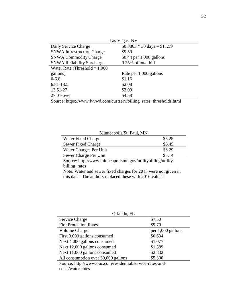
52

Las Vegas, NV

Daily Service Charge $0.3863 * 30 days = $11.59

SNWA Infrastructure Charge $9.59

SNWA Commodity Charge $0.44 per 1,000 gallons

SNWA Reliability Surcharge 0.25% of total bill

Water Rate (Threshold * 1,000

gallons) Rate per 1,000 gallons

0-6.8 $1.16

6.81-13.5 $2.08

13.51-27 $3.09

27.01-over $4.58

Source: https://www.lvvwd.com/custserv/billing_rates_thresholds.html

Minneapolis/St. Paul, MN

Water Fixed Charge $5.25

Sewer Fixed Charge $6.45

Water Charges Per Unit $3.29

Sewer Charge Per Unit $3.14

Source: http://www.minneapolismn.gov/utilitybilling/utility-

billing_rates

Note: Water and sewer fixed charges for 2013 were not given in

this data. The authors replaced these with 2016 values.

Orlando, FL

Service Charge $7.50

Fire Protection Rates $9.70

Volume Charge per 1,000 gallons

First 3,000 gallons consumed $0.634

Next 4,000 gallons consumed $1.077

Next 12,000 gallons consumed $1.589

Next 11,000 gallons consumed $2.832

All consumption over 30,000 gallons $5.300

Source: http://www.ouc.com/residential/service-rates-and-

costs/water-rates

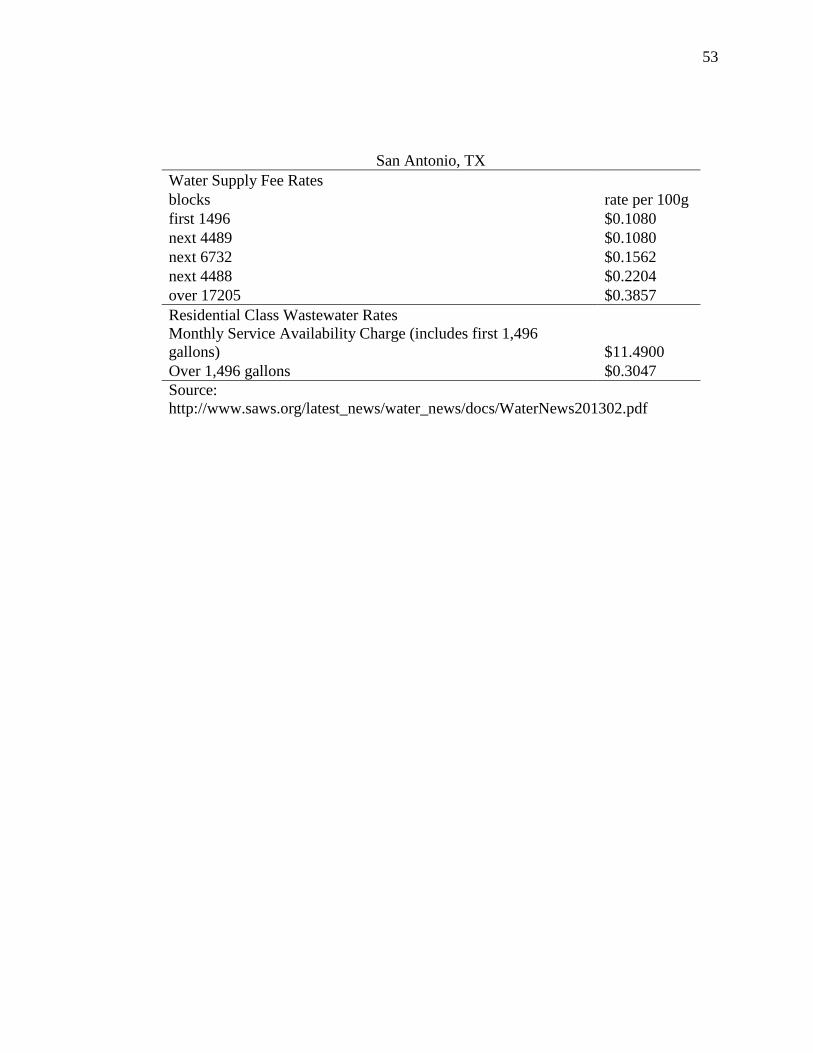
53

San Antonio, TX

Water Supply Fee Rates

blocks rate per 100g

first 1496 $0.1080

next 4489 $0.1080

next 6732 $0.1562

next 4488 $0.2204

over 17205 $0.3857

Residential Class Wastewater Rates

Monthly Service Availability Charge (includes first 1,496

gallons) $11.4900

Over 1,496 gallons $0.3047

Source:

http://www.saws.org/latest_news/water_news/docs/WaterNews201302.pdf

54

Appendix E

DETERMINING USABLE HOUSEHOLDS THAT DO NOT PAY FOR

WATER

There are 18,890 households in Group 2. After we filter out 8,867 households that have

one or more missing variables (not include AMTW), we are left with 10,023 households.

Also, we filter out 467 households that answer 2 in METRO or 3 in TENURE and this

leaves us with 9,556 households. Last, we filter out 371 households that reported negative

or 0 income so the final number of households is 9,185.