Working Paper No. 02-05

The Phillips Curve, the NAIRU, and unemployment asymmetries

William Mitchell and Joan Muysken1

June 2002

Centre of Full Employment and Equity The University of Newcastle, Callaghan NSW 2308, Australia

Home Page: http://e1.newcastle.edu.au/coffee Email: coffee@newcastle.edu.au

2

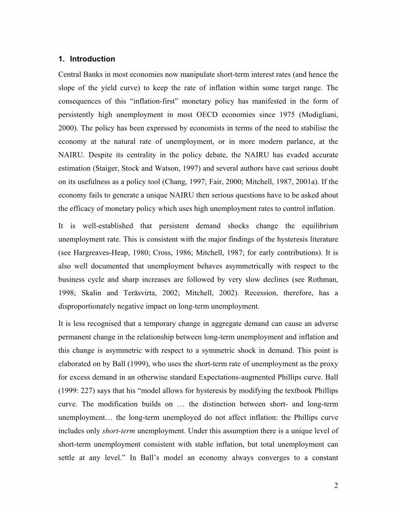
1. Introduction

Central Banks in most economies now manipulate short-term interest rates (and hence the

slope of the yield curve) to keep the rate of inflation within some target range. The

consequences of this “inflation-first” monetary policy has manifested in the form of

persistently high unemployment in most OECD economies since 1975 (Modigliani,

2000). The policy has been expressed by economists in terms of the need to stabilise the

economy at the natural rate of unemployment, or in more modern parlance, at the

NAIRU. Despite its centrality in the policy debate, the NAIRU has evaded accurate

estimation (Staiger, Stock and Watson, 1997) and several authors have cast serious doubt

on its usefulness as a policy tool (Chang, 1997; Fair, 2000; Mitchell, 1987, 2001a). If the

economy fails to generate a unique NAIRU then serious questions have to be asked about

the efficacy of monetary policy which uses high unemployment rates to control inflation.

It is well-established that persistent demand shocks change the equilibrium

unemployment rate. This is consistent with the major findings of the hysteresis literature

(see Hargreaves-Heap, 1980; Cross, 1986; Mitchell, 1987; for early contributions). It is

also well documented that unemployment behaves asymmetrically with respect to the

business cycle and sharp increases are followed by very slow declines (see Rothman,

1998; Skalin and Teräsvirta, 2002; Mitchell, 2002). Recession, therefore, has a

disproportionately negative impact on long-term unemployment.

It is less recognised that a temporary change in aggregate demand can cause an adverse

permanent change in the relationship between long-term unemployment and inflation and

this change is asymmetric with respect to a symmetric shock in demand. This point is

elaborated on by Ball (1999), who uses the short-term rate of unemployment as the proxy

for excess demand in an otherwise standard Expectations-augmented Phillips curve. Ball

(1999: 227) says that his “model allows for hysteresis by modifying the textbook Phillips

curve. The modification builds on … the distinction between short- and long-term

unemployment… the long-term unemployed do not affect inflation: the Phillips curve

includes only short-term unemployment. Under this assumption there is a unique level of

short-term unemployment consistent with stable inflation, but total unemployment can

settle at any level.” In Ball’s model an economy always converges to a constant

3

equilibrium rate of short-term unemployment after employment is disturbed by an

aggregate demand shock. From a policy perspective, if the dynamics implied by Ball

(1999) are empirically robust, then aggregate demand stimulation by government during

a recession can prevent a permanent rise in unemployment without a major cost in

inflation. In addition, the uniqueness of this level of short-term unemployment depends

on other behavioural aspects of the inflationary process, in particular whether the

estimated models are homogenous with respect to expectations and whether the steady-

state unemployment rate is cyclically responsive (see Fair, 2000; Mitchell, 2001a).

Ball (1999: 240) says “hysteresis is reversible: a demand expansion can reduce the

NAIRU” because “they … [employers] … would rather pay the training costs than leave

the jobs vacant” (Ball, 1999: 230). A similar observation underpins the hysteresis models

in Mitchell (1987, 1993). In a high pressure economy, firms lower hiring standards and

address the skill deficiencies of the long-term unemployment by offering on-the-job

training. However, it is not commonly accepted that long-term unemployment is

amenable to cyclical factors. Indeed, the whole thrust of active labour market policy is

predicated on the belief that the long-term unemployed represent a structural bottleneck

that can only be addressed by supply initiatives like training and welfare reform (OECD,

1994, 2001). Layard (1998: 27) argues that “in the very bad old days, people thought that

unemployment could be permanently reduced by stimulating aggregate demand … This

belief has died everywhere … these ideas did not address the fundamental problem: to

ensure that inflationary pressures do not develop while there are still massive pockets of

unemployed people … The only way to address this problem is to make all the

unemployed attractive to employers … Nothing else will do the trick.”2

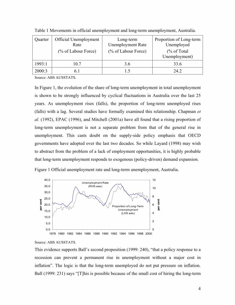
The evidence from the last expansion in Australia is very clear and is shown in Table 1.

The first observation is from the trough of the last recession (1993:1) and the second

(2000:3) represents the peak of the subsequent (long) expansion. Over this robust growth

period, annual trend inflation remained below 3 percent. The proportion of long-term

unemployment fell in lock step with the declines in the official unemployment rate

(although underemployment rose, see Mitchell and Carlson, 2001). The strong demand

led contraction in long-term unemployment provides no adverse inflationary impacts.

4

Table 1 Movements in official unemployment and long-term unemployment, Australia.

Quarter Official Unemployment Rate

(% of Labour Force)

Long-term Unemployment Rate (% of Labour Force)

Proportion of Long-term Unemployed (% of Total

Unemployment) 1993:1 10.7 3.6 33.6 2000:3 6.1 1.5 24.2 Source: ABS AUSSTATS.

In Figure 1, the evolution of the share of long-term unemployment in total unemployment

is shown to be strongly influenced by cyclical fluctuations in Australia over the last 25

years. As unemployment rises (falls), the proportion of long-term unemployed rises

(falls) with a lag. Several studies have formally examined this relationship. Chapman et

al. (1992), EPAC (1996), and Mitchell (2001a) have all found that a rising proportion of

long-term unemployment is not a separate problem from that of the general rise in

unemployment. This casts doubt on the supply-side policy emphasis that OECD

governments have adopted over the last two decades. So while Layard (1998) may wish

to abstract from the problem of a lack of employment opportunities, it is highly probable

that long-term unemployment responds to exogenous (policy-driven) demand expansion.

Figure 1 Official unemployment rate and long-term unemployment, Australia.

0,0

5,0

10,0

15,0

20,0

25,0

30,0

35,0

40,0

1978 1980 1982 1984 1986 1988 1990 1992 1994 1996 1998 2000

per c

ent

0

2

4

6

8

10

12

per c

ent

Proportion of Long-Term Unemployment

(LHS axis)

Unemployment Rate(RHS axis)

Source: ABS AUSSTATS.

This evidence supports Ball’s second proposition (1999: 240), “that a policy response to a

recession can prevent a permanent rise in unemployment without a major cost in

inflation”. The logic is that the long-term unemployed do not put pressure on inflation.

Ball (1999: 231) says “[T]his is possible because of the small cost of hiring the long-term

5

unemployed. With this cost, firms prefer the short-term unemployed to the long-term

unemployed, making the latter irrelevant to wage determination, but they prefer to hire

the long-term unemployment rather than hire nobody.” It is thus important to test whether

long-term unemployment put pressure on inflation given that evidence suggests that they

do become re-employed when demand conditions are strong enough.

The relationships between annual inflation and the short-term unemployment rate and the

official unemployment rate, respectively are plotted in Figure 2. One sees that the short-

term unemployment rate varies more in concordance with the annual inflation rate. For

instance the aggregate unemployment rate shows a stronger deviation in the early 1980s

and again around 1993, when compared to short-term unemployment.

Figure 2 Inflation, short-term and long-term unemployment, Australia, 1978-2001

3

4

5

6

7

8

9

10

-2

0

2

4

6

8

10

12

1980 1985 1990 1995 2000

Short-term unemployment rate (LHS)

Annual inflation rate (RHS)

(a) Annual inflation rate and short-term

unemployment rate

5

6

7

8

9

10

11

12

-2

0

2

4

6

8

10

12

1980 1985 1990 1995 2000

Annual inflation rate (RHS)

Official unemployment rate (LHS)

(b) Annual inflation rate and the official

unemployment rate Source: ABS, AUSSTATS.

Ball illustrates his model in a broad brush way for stylised facts that might pertain to a

typical European economy.3 However, he admits that the model has to be elaborated

before it can be tested in any rigorous manner. Section 2 presents a sophisticated version

of the model, incorporating more complex labour market dynamics including the impact

of changes in the labour force and introducing a full specification of the Phillips curve.

We test this model in Section 3 for the Australian economy, which is in many relevant

ways similar to a typical European economy as Figures 1 and 2 also show. Our partial

estimation results allow us to conclude that the hypotheses underlying Ball his model are

broadly consistent with the data and more detailed empirical analysis is indicated. While

6

employment shocks have a symmetric impact on the labour-force participation rate, they

have an asymmetric impact on short-term unemployment. Moreover, the inflationary

process is more sensitive to movements in the short-run unemployment rate rather than

unemployment overall given other factors like import prices. Concluding remarks follow.

2. Ball’s non-linear inflation model

Ball (1999) develops a model based on an Expectations-augmented Phillips curve using

the rate of short-term unemployment as the measure of wage pressure. He argues that a

unique level of short-term unemployment consistent with stable inflation may exist, but

total unemployment can take on any value. Hence the NAIRU, as defined in the

conventional sense, is undetermined. Moreover, since short-term unemployment is

affected in an asymmetric way by employment shocks, the impact of cyclical variations

in employment on inflation is asymmetric too.

The model needs to be extended in at least two ways to make it fit the stylised facts

outlined in the introduction. First, the model ignores the impact of cyclical changes in the

labour force, which represent an extra channel through which changes in employment

affect both short-run unemployment and the rate of inflation. Second, the Phillips curve is

too simplistic and requires further elaboration and theoretical underpinning. In this

section, we extend the model to take these two features into account.

2.1 Labour market dynamics in Ball

The new element in Ball’s analysis is that employment shocks arising from aggregate

demand movements have asymmetric impacts on short-term unemployment, defined as a

spell of unemployment up to 12 months in duration. This follows from the determination

of short-term unemployment, Us (assuming no labour force changes):

(1a) 1 1, 1s t t tU sE E E s− −= ≥ <

(1b) ( )1 1s t t t t tU sE E E E E− −= + − <

s is the job separation rate and E is the level of employment. In the steady-state, Et = Et-1,

which requires that Us = sEt and thus the ratio of Us/E = s.

7

By conducting the analysis in yearly terms Ball (1999) avoids any complications with

data frequencies that are less than annual. To understand Equations (1a) and (1b), in

terms of annual data frequencies, we start with the accounting statement that the change

in unemployment is the sum of inflows into and outflows from unemployment. Inflow in

unemployment is the result of a fixed rate of job separations, s from employment at the

end of last period, Et-1. Outflow from unemployment is at a fixed rate r of Ut-1, which is

the level of unemployment at the end of last period. Thus:

(2a) ( )1 1 1 1 1 11 , , 1t t t t t t tU U sE rU sE r U E E s r− − − − − −= + − = + − ≥ <

This is consistent with Equation (1a) because the inflow in unemployment over the year

constitutes short-term unemployment and the outflow is by construction from long-term

unemployment. Thus we have 1s tU sE −= .4

In the case of declining employment, inflow into unemployment is augmented by

redundancies, by definition equal to the decline in employment, Et-1 – Et. Thus:

(2b) ( ) ( ) ( )1 1 1 1 1 1 1 11t t t t t t t t t t tU U sE E E rU sE E E r U E E− − − − − − − −= + + − − = + − + − <

Given that the inflow in unemployment over the year constitutes short-term

unemployment and the outflow is by construction from long-term unemployment, this is

consistent with Equation (1b). Hence we have: Us = sEt-1 + (Et-1 – Et).5

In both cases, within-year changes in unemployment are neglected. The consequences of

this become clear when we construct the analysis in quarterly terms but still define short-

term unemployment on a yearly basis.6 While Equations (2a) and (2b) remain relevant, it

becomes more plausible to relate inflow into unemployment to employment at the end of

the previous quarter and outflow from unemployment to unemployment at the same time.

To see the consequences for short-term unemployment, we note that in each quarter the

addition to short-term unemployment is given as [ ]1 1,t t tmax sE sE E− − − ∆ . Recursive

substitution from Equations (2a) and (2b) then gives:

(3) 4

1 1 11

1(1 ) , (1 ) (1 )j j j

t j t j t jj

max s r E s r E r E− − −− − + −

=

− − − − ∆ ∑

8

which replaces Equation (1). Comparison of Equations (3) and (1) shows that within-year

movements in unemployment are captured through the presence of the outflow rate r.

2.2 The impact of labour force dynamics

To help him focus on the impact of exogenous employment changes on short-run

unemployment, Ball (1999) abstracts from labour force changes. However, cyclical

labour force participation rate changes are likely to be an important source of variation in

short-term unemployment. In this section, we redress this gap by developing a model that

incorporates the dynamic impacts of labour force changes. To begin, flows from

Employment and Unemployment to Not in the Labour Force (retirements, discouraged

workers, quits) need to be incorporated. Let these flows be at a rate q for employment and

v for unemployment. Then the flows out of the labour force from employment and

unemployment are qEt-1 and vUt-1, respectively. In addition, the exogenous change in the

labour force (for example, due to demographic changes, migration) is defined as X. The

current labour force is then defined as:

(4) 1 1 1t t t tLF LF qE vU X− − −= − − +

The quarterly change in the labour force is 1 1t t tLF X qE vU− −∆ = − − . The flows qEt-1 and

vUt-1 are likely to be different depending on the state of the business cycle. In a growing

economy, vUt-1 will likely to be low and qEt-1 will mainly constitute retirements. In a

downturn, vUt-1 will increase as discouraged workers stop actively searching for the

diminishing job opportunities and qEt-1 will include previously employed workers who

lose their jobs and join the discouraged workers out of the labour force.7

The maximum capacity of employment to absorb the new inflow X is given

by 1t tR E qE −= ∆ + , given that retirements free up existing jobs by qEt-1. Ιt is then clear

that Equation (2a) no longer holds when 0R ≥ , but instead requires 1t tR E qE X−= ∆ + ≥ .

From Equation (4), we know that 1 1t t tX LF qE vU− −= ∆ + + . Therefore the demarcation

condition (between growth and contraction), R X≥ can be written as 1t t tE LF vU −∆ ≥ ∆ + ,

which says that the change in employment has to equal the change in labour force plus

the number of unemployed who dropped out of the workforce.8

9

Equation (2a) is therefore replaced by:

(5a) ( )1 1 1 1 1 1( ) 1t t t t t t t tU U sE r v U sE r v U E LF vU− − − − − −= + − + = + − − ∆ ≥ ∆ +

Since the component of the labour force change that cannot be absorbed by employment

will be added to unemployment, Equation (2b) is similarly replaced by:

(5b) ( ) ( )1 1 1 11t t t t t t tU sE LF vU E r v U E LF vU− − − −= + ∆ + −∆ + − − ∆ < ∆ +

Short-run unemployment is then given by:

(6a) 1 1s t t t tU sE E LF vU− −= ∆ ≥ ∆ +

(6b) ( )1 1s t t t t t tU sE LF vU E E LF vU− −= + ∆ + −∆ ∆ < ∆ +

We can alternatively express short-term unemployment in terms of shocks to

employment and the labour force, R and X, respectively:

(7a) 1s tU sE R X−= ≥

(7b) ( )s tU sE X R R X= + − <

The analysis changes if quarterly data is used but we define short-term unemployment in

annual terms. Clearly, Equations (5a) and (5b) remain relevant. But now the extra short-

term unemployment each quarter is given as [ ]1 1 1, ( )t t t t tmax sE sE LF vU E− − −+ ∆ + −∆ .

Recursive substitution from Equations (5a) and (5b) then gives:9

(8) 14

1 11 1 1

(1 ) ,(1 ) (1 ) ( )

jt j

j jj t j t j t j t j

s r v Emax

s r v E r v LF vU E

−−

− −= − + − − + −

− − − − + − − ∆ + −∆

∑

which replaces Equation (6). Comparing Equations (8) and (6) shows that within-year

movements in unemployment are captured by the outflow rate r and the exit rate v.10

Equation (8) shows that employment shocks have asymmetric impacts on the short term

unemployment rate, as in Equation (1). In our model, the impact is stronger because of

the impact of employment shocks on the labour force.

10

We now seek to determine the impact of employment shocks on the “equilibrium rate of

unemployment” and, in turn, on inflation. To accomplish this task we need to incorporate

these results in the specification of the Phillips curve.11

2.3 A conventional Phillips curve

We begin with a “conventional” approach to the Phillips curve as “the battle between

mark-ups”, which results from imperfectly competitive wage- and price-setting behaviour

(see Carlin and Soskice, 1990). In terms of wage setting behaviour, we seek to model the

impact of unemployment on wages using cU/H, where cU is interpreted as the number of

effective job seekers (c being the average job search effectiveness and U being the total

number of unemployed) and H is the total number of new hires. Assuming flow

equilibrium prevails in the labour market (hence sE = H), we derive cU/H = cu/s with u =

U/E as the rate of unemployment. The wage equation then becomes:

(9) ( )0 1 2/ eww p h cu s p p zβ β β− = + − − − +

where w and p are log of wage costs and output prices, respectively, h is the log of labour

productivity and zw reflects all other factors affecting wage setting. The latter include the

wedge between consumer and output prices and between wage costs and net wages.

Inflation surprises ( )ep p− have a negative impact on the bargained real wage.

We can rewrite the wage equation in terms of the labour share in national income:12

(10) ( )0 1 2/ eww p h cu s p p zβ β β− − = − − − +

In the conventional approach, firm wage setting behaviour is modelled by combining the

labour demand and price setting behaviour as shown in the Appendix. We then find:

(11) 0 1( )k l pw p h p p zθ θ− − = − − −

Here (pk - pl) represents the impact of the relative price of capital.13 The vector zp reflects

other price setting influences, including the wedge between domestic and foreign prices.

Combining equations (10) and (11) yields the following short-run Phillips curve:

(12) *1 2( / )( / )ep p c s u uβ β = + −

11

with inflation 1t tp p p −= − and ep is expected inflation as before, and:

(13) *1 0 0 1(1/ ) ( ) ( / )k l w pu p p z z s cβ β θ θ = − + − + +

u* can be interpreted as the NAIRU or “equilibrium rate of unemployment”. Equation

(13) shows that the NAIRU increases with wage- and price-push factors, as is elaborated

in Layard et al. (1991). It also increases when the price of capital increases relative to that

of labour, as is emphasised by Phelps (1994) and Blanchard (1999). Finally it increases

when the average rate of search effectiveness c decreases, as is also elaborated in Layard

et al. (1991). The latter is interesting from the point of view of the analysis of Ball

(1999), since in his view search effectiveness is affected by the state of the labour market.

2.4 Modelling search effectiveness

Ball (1999) identifies cU with short-term unemployment and hence from Equation (5) we

find:14,15

(14) [ ]/ max 1 ,1 / ( / ) (1 )E E LFcu s g g s r s g u= − − + +

where gLF represents the rate of labour force growth. As a consequence and consistent

with Ball (1999), search effectiveness c relative to the rate of separation s is given by:

(15) [ ]/ (1/ ) max 1 ,1 / ( / ) (1 )E E LFc s u g g s r s g u= − − + +

If we assume a steady-state situation where employment grows at the rate * 0Eg > and

unemployment is at u* we find that:16

(16) * */ (1/ )(1 )Ec s u g= −

Substitution of this result into Equation (11) yields:

(17) *1 0 0 11 (1/ ) ( )E k l w pg p p z zβ β θ θ = − − + − + +

While consistent with the conclusion of Ball (1999) that the steady-state unemployment

rate u* is undetermined, we would note instead that employment growth should satisfy

(17). The intuition is that only short-term unemployment matters and this is determined

12

by employment growth. Long-term unemployment can take any value, without having an

impact on inflation.

The equilibrium rate of short-term unemployment can be found from * *su cu= , with u*

given by Equation (13):

(18) *1 0 0 1(1/ ) ( )s k l w pu s p p z zβ β θ θ = − + − + +

So the factors that normally affect the NAIRU in an extended specification of the Phillips

curve, now only affect the equilibrium rate of short-term unemployment.

3. Estimation and results

In this section, we subject the theoretical model and its underlying hypotheses to some

empirical analysis. We do not estimate nor test the model simultaneously nor do we

compute the labour flow parameters directly.17 We present separate estimations for the

impact of employment shocks on the labour force following Equation (4) and for short-

run unemployment following Equation (8). We finally use a short-run Phillips curve to

examine the claim that short-term unemployment is a more effective measure of demand

pressure than the official unemployment rate following Equation (14).

The data sources and construction of variables are outlined in detail in the Data

Appendix. The time series properties of the data are presented in Table 2. These

properties were initially examined using Augmented Dickey-Fuller (ADF) tests and

Kwiatkowski-Phillips-Schmidt-Shin (KPSS) tests, which provide some contrast because

in the former case the null is that the time series contains a unit root, whereas in the

KPSS test, trend-stationarity is the null. A constant and trend term were included and the

lag order was determined using the AIC statistic. The inconsistency of the results when

the null is reversed is evident. In general, the inflation variables (prices, import prices)

used in the Phillips curve estimation are expressed as annualised differences and are

likely to be stationary, and the unemployment rate terms (given they are bounded from

above and below) are assumed to be stationary by construction. Any finding consistent

with the presence of a unit root in the unemployment terms points to the low power of the

tests given a finite sample. The employment terms used in this section are also marginally

inconclusive.

13

Table 2 Unit root tests for model variables, Australia, 1978:1 to 2001:4

Unit Root Null Trend Stationary Null ADF KPSS t-stat LM Price level -1.131 0.323 Annual inflation -4.213 0.083 Import price level -2.228 0.297 Annual import price inflation -8.669 0.073 Short-term unemployment -3.234 0.110 Change in short-term unemployment -4.303 0.042 Unemployment -3.011 0.134 Change in unemployment rate -3.648 0.041 Employment -3.329 0.067 Change in Employment -3.518 0.046 Critical Values 1% level -4.058 0.216 5% level -3.458 0.146 10% level -3.155 0.119

Source: Critical values from Kwiatkowski-Phillips-Schmidt-Shin (1992, Table 1)

3.1 Cyclical sensitivity of the labour force participation rate

It is well documented that the labour force participation rate displays cyclical variability

(Mitchell, 2001b). Discouraged workers, for example, are said to exit the labour force

when employment opportunities are sparse despite remaining willing to work. They

return to the labour force when employment opportunities improve. The alternative added

worker phenomenon describes the entry of marginal workers into the labour force to

supplement family income when the labour market deteriorates and exit when the

incomes of the primary breadwinner improve. Empirical studies suggest that the

discouraged worker effect dominates (see evidence in Mitchell, 2001b).

14

This response is depicted in Figure 3 for Australia using quarterly data over the period

1966 to 2001. The data was divided into the two regimes according to Equations (7a) and

(7b). The triangular plot symbols correspond to R < X. Simple linear trends are shown for

observations corresponding to each regime. Graphically, the responsiveness of changes in

the labour force participation rate (LFPR) seems to be largely symmetrical across the two

regimes.

Figure 3 Relationship between employment growth and changes in LFPR, 1966-2001

-0.008

-0.006

-0.004

-0.002

0.000

0.002

0.004

0.006

0.008

-1.5 -1 -0.5 0 0.5 1 1.5 2

Source: ABS AUSSTATS.

We regress the change in the labour force participation rate on employment growth (both

sorted according to regimes noted above) and Chow’s breakpoint and predictive failure

test statistics computed to correspond with the regime break in the sorted series. Both

tests fail to reject the null that the labour force participation response is symmetric.

We thus assume that labour force participation rate changes, ∆lfpr responds

symmetrically to the business cycle with a factorφ and also increases autonomously by

∆lfpr* percentage points. As a consequence we specify:

(19) * *( )t E Elfpr g g lfprφ∆ = − + ∆

with gE as employment growth and gE* is trend employment growth. The new entrants

and re-entrants to the labour market then are given by:

(20) 1 1 1( )t t t t tLF lfpr P lfpr lfpr P− − −∆ = ∆ + + ∆ ∆

15

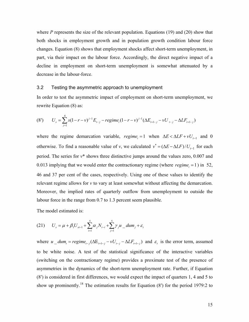
where P represents the size of the relevant population. Equations (19) and (20) show that

both shocks in employment growth and in population growth condition labour force

changes. Equation (8) shows that employment shocks affect short-term unemployment, in

part, via their impact on the labour force. Accordingly, the direct negative impact of a

decline in employment on short-term unemployment is somewhat attenuated by a

decrease in the labour-force.

3.2 Testing the asymmetric approach to unemployment

In order to test the asymmetric impact of employment on short-term unemployment, we

rewrite Equation (8) as:

(8′) 4

1 11 1

1

(1 ) (1 ) ( )j js t j i t j t j t j

j

U s r v E regime r v E vU LF− −− + − − + −

=

= − − − − − ∆ − −∆∑

where the regime demarcation variable, 1iregime = when 1tE LF vU −∆ < ∆ + and 0

otherwise. To find a reasonable value of v, we calculated *1( ) / tv E LF U −= ∆ −∆ for each

period. The series for v* shows three distinctive jumps around the values zero, 0.007 and

0.013 implying that we would enter the contractionary regime (where 1iregime = ) in 52,

46 and 37 per cent of the cases, respectively. Using one of these values to identify the

relevant regime allows for v to vary at least somewhat without affecting the demarcation.

Moreover, the implied rates of quarterly outflow from unemployment to outside the

labour force in the range from 0.7 to 1.3 percent seem plausible.

The model estimated is:

(21) 5 5

1 11 1

_s st j t i j j ti j

U U N u dumµ β α γ ε− −= =

= + + + +∑ ∑

where 1 1_ ( )t t j t j t j t ju dum regime vU LF− + − − + −= ∆Ε − −∆ and tε is the error term, assumed

to be white noise. A test of the statistical significance of the interactive variables

(switching on the contractionary regime) provides a proximate test of the presence of

asymmetries in the dynamics of the short-term unemployment rate. Further, if Equation

(8′) is considered in first differences, we would expect the impact of quarters 1, 4 and 5 to

show up prominently.18 The estimation results for Equation (8′) for the period 1979:2 to

16

2001:4 are shown in Table 3 for v* = 0.013. This value yielded the best estimation results

as judged by the standard error of estimate of the regression.

Table 3 Estimating asymmetric effects of employment change on short-term unemployment, Australia, 1979:2 to 2001:3.

Dependent Variable: STU Coefficient Estimate (t-statistic)

Constant -0.72 (0.08)

STU(t-1) 0.97 (51.01)

N(t-1) 0.01 (0.38)

N(t-2) -0.03 (0.84)

N(t-3) -0.02 (0.57)

N(t-4) 0.09 (2.17)

N(t-5) -0.04 (1.39)

u_dum(t-1) -0.96 (17.8)

u_dum(t-2) 0.12 (1.89)

u_dum(t-3) 0.05 (0.87)

u_dum(t-4) 0.15 (2.31)

u_dum(t-5) 0.09 (1.36)

R-squared 0.99

S.E. as % of mean of dependent variable 1.91

The hypothesis that β1 = 1 cannot be rejected and so the model can be simplified in first-

difference form. Moreover, the dummy variables are jointly significant with a formal test

strongly rejecting the hypothesis that the impact of all u_dum is zero. This provides

support for the view that asymmetries are important in explaining the changes in short-

17

term unemployment. Finally, the high value of the one-quarter lagged dummy variable

implies that in the first quarter, almost all excess supply is added to short-term

unemployment when 1tLF vU −∆Ε < ∆ + . This is fully consistent with the reasoning

developed above.19

While not conclusive, the results of this section suggest that the short-term

unemployment dynamics for Australia are consistent with our formal model.

3.3 Phillips curve analysis

In this section, we utilise the measure of short-term unemployment available from the

ABS Labour Force Survey, assuming that the asymmetries behave as suggested in

Equations (6a) and (6b) are already incorporated in the extant data. We thus estimate the

Phillips curve of equation (12) independent of the other equations.

Four major contentions are examined:

1. Does the short-term unemployment rate provide a stronger constraint on the annual

inflation rate relative to the overall unemployment rate? We expect the coefficient on

the short-term unemployment rate in a Phillips curve model to be larger in absolute

value and negatively signed when compared with coefficients corresponding to other

unemployment measures.

2. Does the long-term unemployment rate exert any statistically significant impact on

the annual inflation rate? We expect the coefficient on the long-term unemployment

rate in a Phillips curve model to be statistically insignificant.

3. Does the TV-NAIRU model of the evolution of excess demand provide an inferior

explanation of the inflation process compared to the models developed under

hypothesis (1)? We expect an inflation models using the gap between the short-term

unemployment and its filtered trend to be superior to that which uses the gap between

the official unemployment rate and its filtered trend as the excess demand measure.

The latter variable is typically used in TV-NAIRU studies (see Mitchell, 2001a).

4. Does the estimated Phillips curve exhibit NAIRU dynamics? Fair (2000) and Mitchell

(2001a) present tests based on the coefficients on the lagged dependent inflation

18

variable to determine whether the inflation dynamics are consistent with a constant

NAIRU model. The test is a simple homogeneity test on the lagged inflation terms.

We use a general autoregressive-distributed lag Phillips curve representation like:

(22) 1 0 0

qn m

t i t i i t i i t i ti i i

p p u zα δ β γ ε− − −= = =

= + + + +∑ ∑ ∑

where tp is the rate of inflation at time t, u is the unemployment rate, z is a cost shock

variables (like import price inflation, capital costs), and the ε is a white-noise error term.

In addition, the u variable can take the form of the aggregate unemployment rate or the

short-term unemployment rate to facilitate the testing of the hypotheses (1) to (3) outlined

above. In the case of hypothesis (3) we compute UR* and STUR* using a Hodrick-

Prescott (HP) filter on the official unemployment rate, UR and the short-term

unemployment rate, STUR, respectively. The variables (UR - UR*) and (STUR - STUR*)

are the original series less the HP filtered trend series in each case.

Further, if the δ coefficients sum to unity, the model gives a constant NAIRU

of0

m

iiα β

=− ∑ . At this unemployment rate, the inflation rate will only exhibit short-run

changes due to changes in changes in z and/or random shocks (changes in ε). So we can

test hypothesis (4) by testing for homogeneity.

We initially develop a Phillips curve model for Australia using Equation (22) using 4 lags

on the annualised inflation terms (D4LP) and import prices (D4LPM), the level of the

unemployment rate, a dummy variable, DGST (defined as 1 in 2000:3 and zero

otherwise) to take into account the introduction of the Goods and Services Tax system in

Australia in July 2000, and other variables capturing the cost of capital, interest spread,

and payroll taxes and the like. The other variables were not retained in the final tested-

down specification. Sequential testing down from the general equation using different

measures of the unemployment variable yielded the results shown in Table 4. In each

case, the dynamics were so close and the coefficient estimates for the other variables

were highly stable that a common specification is employed, which aids comparison

considerably. The diagnostics of all equations were satisfactory.

19

Equation (1) in Table 4 describes a typical Phillips curve using the aggregate

unemployment rate (UR). The unemployment rate exerts a negative influence on the rate

of inflation (-0.18). A comparison with Equation (2) which splits the unemployment rate

into short-term and long-term components shows that the LTUR is not statistically

significant (even at the 10 per cent level). Further, the degree of negative pressure on

inflation exerted by the highly significant STUR rises to -0.53, substantially above that

estimated for UR. Equations (3) and (4) are inferior specifications and warrant no specific

comment.

Mitchell (2002) argues that the NAIRU concept remains on shaky theoretical grounds.

Importantly, the original theory underpinning the NAIRU provides no guidance about its

evolution although, we would be looking to the evolution of unspecified structural factors

to remain faithful to that theory. In this theoretical void, econometricians have used

techniques that allow for a smooth evolution although there is no particular

correspondence with any actual economic factors. Some authors assert that a Hodrick-

Prescott filter through the actual series captures the TV-NAIRU (for example Boone,

2000 among many). Of-course, the Hodrick-Prescott filter merely tracks the underlying

trend of the unemployment and follows it down just as surely as it follows it up. The

unemployment rate is highly cyclical and the TV-NAIRU proponents are silent on this

apparent anomaly – why do the alleged structural factors cycle with the actual rate?

Equations (5) and (6) use the alternative form of the unemployment variables in terms of

the actual value (of UR and STUR) being expressed as gaps on their respective filtered

trend values. These regressions constitute an improvement on (1) to (4). Equation (5) is

thus in the TV-NAIRU vein and performs reasonably in statistical terms. The coefficient

on the demand pressure gap (UR - UR*) is -0.409, substantially higher than that estimated

for Equation (1). However, Equation (5) is inferior to Equation (6) that replaces (UR -

UR*) with the short-term unemployment rate gap (STUR - STUR*). This has a lower

standard error of estimate and the deviation of STUR from its current (shifting) HP-

filtered value, STUR* is -0.648. In other words, a 1 per cent deviation above the filtered

value leads to a 0.64 per cent slowdown in the annualised inflation rate.

20

It is interesting to consider the different values of the coefficients on the STUR and UR

variables. They suggest the following dynamics are taking place. An initial downturn

initially increases (according to our model) short-term unemployment, which reduces

inflation because the inflow into short-term unemployment is comprised of those

currently employed and active wage bargaining processes. As the downturn continues,

long-term unemployment starts to rise because some of the unemployed were in their 4th

quarter of short-term unemployment. This progressively becomes the case in a protracted

downturn and the pressure exerted on the wage setting system by unemployment overall

falls. This requires higher levels of short-term unemployment being created to reach low

inflation targets with the consequence of increasing proportions of long-term

unemployment being created.

The results taken together provide strong support for the hypotheses (1) to (3) outlined

above and for the theoretical model developed in Section 2.

An additional finding is that a long-term trade-off between unemployment and inflation is

implied in all regressions. The NAIRU dynamics test statistic shown in Table 4 allows us

to easily reject the null that the sum of the coefficients on the lagged inflation terms is

unity in all regressions. In that sense, we would reject the constant NAIRU hypothesis.20

So even though the short-term unemployment rate is relatively more effective in

controlling inflation, there is no convergence to a constant equilibrium rate of short-term

unemployment after an employment shock. The transitory equilibrium short-term

unemployment rate is contingent on the evolution of employment growth and demand in

general. In the next paper we will demonstrate that our estimation results confirm that

even a temporary change in demand causes an adverse permanent change in inflation and

this change is asymmetric with respect to a symmetric shock in demand. Combined with

the other findings relating to hypotheses (1) to (3) and the underlying model in Section 2,

we interpret these results as being consistent with a hysteretic vision of the inflationary

dynamics in Australia. The results indicate that a deflationary strategy using demand

repression (tight monetary and fiscal policy) will be costly in terms of unemployment.

These results are also consistent with the findings of other studies (Franz, 1987; Mitchell,

1987, 1993) and support the conceptual underpinning of the main hypothesis in Ball

21

(1999). One may therefore conclude “that increases in the NAIRU in most countries have

come disproportionately from increases in long-term unemployment” Ball (1999: 40).

Table 4 Phillips curve regressions, Australia, 1978:1 to 2001:4

(1) (2) (3) (4) (5) (6)

UR STUR-LTUR STUR LTUR URGAP STURGAPConstant 0.02 0.02 0.02 0.01 0.00 0.00 (2.96) (3.77) (3.53) (1.91) (1.62) (1.21) ∆4LP(-1) 0.88 0.93 0.90 0.88 0.89 0.91 (29.4) (25.6) (32.9) (25.4) (32.9) (35.1) UR -0.18 (2.84) UR-UR* -0.409 (4.10) STUR -0.53 -0.35 (3.22) (3.42) STUR-STUR* -0.648 (4.53) LTUR 0.30 -0.25 (1.36) (1.72) ∆4LPM 0.05 0.05 0.05 0.05 0.06 0.06 (4.13) (4.31) (4.26) (3.94) (4.98) (4.83) DGST 0.02 0.02 0.02 0.02 0.02 0.02 (2.46) (2.49) (2.43) (2.60) (2.63) (2.72)

R-Squared 0.94 0.95 0.94 0.94 0.95 0.95 S.E. of regression 0.00814 0.00796 0.00821 0.00836 007806 0.00767 se % mean 15.0 14.7 15.1 15.4 14.4 14.1 SC LM(1) 2.24 0.35 0.47 3.51 0.50 0.06 ARCH 4) 0.49 0.99 0.70 0.38 0.51 0.88 RESET(2) F 0.10 0.09 0.04 0.12 0.35 0.19

NAIRU dynamics test

F-statistic 14.9 3.3 15.3 11.0 16.3 13.1 d.f. (1,90) (1, 90) (1, 92) (1, 91) (1,91) (1,91) Prob-value 0.0000 0.0711 0.0002 0.0013 0.0001 0.0005

Notes: SC LM(1) is a Breusch-Godfrey Serial Correlation 1st order LM Test, ARCH(4) is a 4th order test for Autoregressive conditional heteroscedasticity, RESET(2) is the Ramsey RESET test with 2 added terms, t-statistics are in parentheses. UR* and STUR* were computed using a Hodrick-Prescott filter on the UR and STUR, respectively. The variables UR-UR* and STUR-STUR* are the original series less the HP filtered trend series in each case.4.

22

4. Conclusion

In this paper we have presented a sophisticated version of the Ball (1999) model, which

uses the dynamics of short-term unemployment to show that a temporary change in

aggregate demand can cause an adverse permanent change in the relationship between

long-term unemployment and inflation and this change is asymmetric with respect to a

symmetric shock in demand. We incorporate more complex labour market dynamics,

including the impact of changes in the labour force, in the model and introduce a full

specification of the Phillips curve. The distinction between short- and long-term

unemployment allows the differential impact of each on inflation to be assessed. The

essential results remain that the equilibrium unemployment rate is dependent on the state

of the business cycle and the long-term unemployed do not exert a significant negative

influence on the inflation rate.

The convergence to a short-term unemployment does not mean that there is a unique

NAIRU if the long-term unemployed do not affect inflation. From a policy perspective,

the dynamics implied by Ball (1999) allow aggregate demand stimulation by government

during a recession to prevent a permanent rise in unemployment without a major cost in

inflation. Ball (1999) also argues that hysteresis is reversible and the long-term

unemployed can be reabsorbed in a non-inflationary manner back into employment if

aggregate spending is strong enough. This model poses major problems for the supply-

side orthodoxy, which posits that the long-term unemployed represent a structural

bottleneck and only supply initiatives like training and welfare reform can be effective.

The empirical modelling provides strong support for the theoretical model and suggests

further research is needed to more precisely estimate the labour market flows that

underpin it. While employment shocks have a symmetric impact on the labour-force

participation rate, the have an asymmetric impact on short-term unemployment.

Moreover, the inflationary process is more sensitive to movements in the short-run

unemployment rate rather than the aggregate unemployment rate. The results are also

consistent with other evidence presented that long-term unemployment can be reduced by

creating more employment overall without fears of an accelerating inflation rate.

23

Data Appendix

Inflation measure

The annual inflation rate is expressed as the four-quarter log change in the Consumer

Price Index taken from the ABS TRYM database.

Import price index

The import price index is expressed as the four-quarter log change in the TRYM Model

Import Price Index (1990/91 = 1) taken from the ABS TRYM database.

Labour Market Variables

All the labour force data are taken from the ABS Time Series Service available via

AUSSTATS. The short-term unemployment rate is computed as official unemployment

minus long-term unemployment expressed as a percentage of the labour force. Long-term

unemployment is defined as a spell of unemployment longer than 52 weeks.

24

Appendix on the derivation of the Phillips curve

The labour demand function assumes that output has a positive impact on labour demand,

while the cost of labour relative to capital has a negative impact. Thus:

(A1) 0 1/ l tl l y p g hα ξ α α α α1 2= + − − − = =

where y and l are log output and demand for labour, respectively, with 1ξ ≥ as the

returns to scale parameter. The efficiency-corrected price for labour is pl, and the price of

capital is pk. We assume that annual wage costs w are corrected for the impact of working

time g and the growth of labour productivity ht. Hence, in log terms:

(A2) l tp w g h= − −

The price of capital relates investment price pi to the nominal interest rate r plus

depreciationδ. For simplicity, we ignore the impact of taxes. Hence, in log terms:

(A3) (k ip p r δ= + + )

We assume that the output price, p is set as a markup over average costs and that total

costs C allow for economies of scale. Hence:

(A4) 1/1 2with 1 ( / )( / )l k lC cy c k p k a p pξ α = = +

where c represents normal unit costs.21 We approximate these unit costs by a mark-up

over efficiency labour costs, where the mark up depends negatively on the price of labour

relative to capital.22

The price setting equation (a mark-up over average costs) yields the domestic price:

(A5) (1 ) /y cp c yµ ξ ξ= + + −

where µ is the log mark-up and cc is the log unit cost measure. We approximate:23

(A6) c l kc p p lγ γ γ γ γ γ0 1 1 2= + + − = =

Finally output price is a weighted average of domestic price, py, and the price of foreign

competitors, pf, in log terms:

(A7) (1y fp p pϕ ϕ= + − )

25

Combining the labour demand and price equations, (A1) and (A5), respectively, and

using (A6) and (A7), we find:

(A8) ( ) ( )( ) (1 )( )k l y fw p h p p p pα µ γ γ α ϕ0 0 1 1− − = − − − − − + − −

26

References

Ball, L. (1999) ‘Aggregate Demand and Long-Run Unemployment’, Brookings Papers on Economic Activity, 2, 189-251.

Ball, L. and Mankiw, N.G. (2002) ‘The NAIRU in Theory and Practice’, forthcoming Journal of Economic Perspectives.

Blanchard, O.J. (1999) ‘European Unemployment: the Role of Shocks and Institutions’, Baffi Lecture, Rome.

Blanchard, O.J. and Wolfers, J. (2000) ‘The Role of Shocks and Institutions in the Rise of European Unemployment: The Aggregate Evidence’, Economic Journal, March, C1-C33.

Boone, L. (2000), “Comparing Semi-Structural Methods to Estimate Unobserved Variables: The HPMV and Kalman Filters Approaches”, Economics Department Working Papers No. 240, OECD, Paris.

Carlin, W. and Soskice, D. (1990) Macroeconomics and the Wage Bargain, Oxford University Press, Oxford.

Chang, R. (1997) ‘Is Low Unemployment Inflationary?’, Federal Reserve Bank of Atlanta, Economic Review, First Quarter.

Chapman, B.J., Junanker, P.N. and Kapuscinski, C.A. (1992) ‘Long Term Unemployment: Projections and Policy’, Discussion Paper No. 274, Centre for Economic Policy Research, Australian National University, Canberra.

Cross, R. (1986) ‘Phelps, Hysteresis and the Natural Rate of Unemployment’, Quarterly Journal of Business and Economics, 25, 1, Winter, 56-64.

Economic Planning and Advisory Commission (EPAC) (1996) Future labour market issues for Australia, Commission Paper No. 12, (AGPS: Canberra).

Fair, R. (2000) ‘Testing the NAIRU Model for the United States’, The Review of Economics and Statistics, February, 64-71.

Franz, W. (1987) ‘Hysteresis, Persistence and the NAIRU: An Empirical Analysis for the Federal Republic of Germany’, in Layard, R. and Calmfors, L (eds.), The Fight Against Unemployment, MIT Press, Cambridge.

Hargreaves-Heap, S.P. (1980) ‘Choosing the Wrong “Natural” Rate: Accelerating Inflation or Decelerating Employment and Growth?’, The Economic Journal 90, 611-20.

Kwiatkowski, D., Phillips, P.C.B., Schmidt, P. and Shin, Y. (1992) ‘Testing the Null Hypothesis of Stationarity Against the Alternative of a Unit Root: How Sure Are We that Economic Series Have a Unit Root’, Journal of Econometrics 54, 159-178.

Layard, R. (1998) ‘Getting People Back to Work’, Centrepiece Magazine, Autumn, 24-27.

Layard, R., Nickell, S. and Jackman, R. (1991) Unemployment, Macroeconomic Performance and the Labour Market, Oxford University Press, Oxford.

27

Mitchell, W.F. (1987) ‘The NAIRU, Structural Imbalance and the Macroequilibrium Unemployment Rate’, Australian Economic Papers, 26, 48, 101-118.

Mitchell, W.F. (1993) ‘Testing for Unit Roots and Persistence in OECD Unemployment Rates’, Applied Economics, 25, 1489-1501.

Mitchell, W.F. (2001a) ‘The unemployed cannot find jobs that are not there!’, in Mitchell, W.F. and Carlson, E. (eds.), Unemployment: the tip of the iceberg, CAER-UNSW Press, Sydney.

Mitchell, W.F. (2001b) ‘Hidden unemployment in Australia’, in Mitchell, W.F. and Carlson, E. (eds.) Unemployment: the tip of the iceberg, CAER-UNSW Press, Sydney, 33-46.

Mitchell, W.F. (2002) ‘Non-linearity in unemployment and demand side policy for Australia, Japan and the US’, Working Paper 02-02, Centre of Full Employment and Equity, The University of Newcastle, April.

Mitchell, W.F. and Carlson, E. (2001) ‘Labour underutilisation in Australia and the USA’ in Mitchell, W.F. and Carlson, E. (eds.) Unemployment: the tip of the iceberg, CAER-UNSW Press, Sydney, 47-68.

Mitchell, W.F., Muysken, J. and Watts, M.J. (2002) ‘Wage and productivity relationships in Australia and the Netherlands’, Paper presented to AIRAANZ Conference, Queenstown, New Zealand, February.

Modigliani, F. (2000) ‘Europe's Economic Problems’, 3rd Monetary and Finance Lecture Freiburg No. Carpe Oeconomiam Papers in Economics, April 6.

OECD (1994) The Jobs Study, Organisation for Economic Co-operation and Development, Paris.

OECD (2001) Innovations in Labour Market Policies, The Australian Way, Organisation for Economic Co-operation and Development, Paris.

Phelps, E. (1994) Structural slumps: The Modern Theory of Unemployment, Interest and Assets, Harvard University Press, Cambridge.

Rothman, P. (1998), “Forecasting asymmetric unemployment rates”, Review of Economics and Statistics, 80, 164-168.

Skalin, J. and Teräsvirta, T. (2002) ‘Modelling asymmetries and moving equilibria in unemployment rates’, Macroeconomic Dynamics, forthcoming. Staiger, D., Stock, J.H., and Watson, M.W. (1997) ‘The NAIRU, Unemployment and Monetary Policy’, Journal of Economic Perspectives, 11(1), 33-49.

28

Notes

1 The authors are Professor of Economics and Director of the Centre of Full Employment and Equity, The University of Newcastle; and Professor of Economics and Director, CofFEE-Europe, respectively. 2 Layard (1998) underpins his argument with a major assertion that new jobs follow an increase in the effective labour supply. In what represents a modern restatement of Say’s Law and the efficacy of the real balance effect, he says (1998: 26) “the mechanism is simple enough. If the labour supply increases and the number of jobs does not, inflation starts to fall; this makes possible an increase in aggregate demand in the economy, which in turn increases employment in line with the increase in the labour supply.” It is a pity that OECD economies in general have not witnessed these dynamics over the last 25 years. 3 Ball and Mankiw (2002), for example, argue that the model of Ball (1999) does not apply to the US economy. 4 Since Ut is the stock at the end of period t, the outflow rUt-1 refers to long-term unemployed who were already unemployed a year ago. On the other hand, the inflow sEt-1 accumulates during the current period and by definition constitutes short-term unemployment. 5 We ignore here the subtle point that separations can be related to Et instead of Et-1, in case of redundancies. The correct specification lies somewhere in between both. When quarterly data is employed this difference is not important. 6 When short-term unemployment is defined as unemployed for a quarter or less, the analysis with quarterly data can be applied without any modification to equations (3) and (4). 7 This also suggests that v will increase in a down turn, hence behaves counter cyclical, whereas q will behave pro cyclical. 8 Given ∆E = ∆LF – ∆U this condition amounts to 1t tU vU −∆ ≤ . 9 Due to the interaction between various labour markets, the regime change in the labour market will likely be less strict than indicated by the demarcation ∆LF + qLFt-1 = ∆E. We ignore this complexity in this paper. 10 As is the case with v and q, the rates s and r may vary counter- and pro-cyclically, respectively. This can be accounted for by modelling these rates in terms of detrended employment growth. 11 We use the term “equilibrium unemployment rate” to denote the unemployment rate that is associated with stable inflation. We do not impute any particular temporal significance to this rate and assume that hysteresis is the dominant process operating to determine this relationship (Mitchell, 1987). 12 While this is an accounting construction, the imposition of behavioural assumptions on the model assumes that workers are able to translate labour productivity growth into proportionate changes in real wages growth. Evidence shows that this may not be the case (see Mitchell, Muysken and Watts, 2002). 13 See for example, Blanchard (1999); Blanchard and Wolfers (2000), and Phelps (1994). 14 One should remember that cu/s originally was cU/sE, which now becomes Us/sE. We assume here that when gE is negative, 1 – gE is always dominated by 1 - gE /s + (r/s).gLF.(1 + u). 15 For expositional simplicity we use the yearly representation of labour market flows. Hence we ignore the impact of quarterly dynamics. 16 The unemployment rate u* is the only rate consistent with the steady-state and, hence, constant inflation. 17 In a later paper we will use Gross Flows data (currently unavailable) to compute the unknown flow parameters more precisely and to accurately compute Equation (8) and then estimate the model as a system.

29

18 The variables in between do not necessarily disappear, since the rates s, r and v may show cyclical variations. 19 This also holds for the finding that the coefficients for N(t-1) to N(t-5) add up to unity. 20 Mitchell (2001a) tested for NAIRU dynamics in similarly derived Phillips curve models for Canada, France, Germany, Italy, Japan, the United Kingdom, and the United States. There was no evidence of a constant NAIRU operating in these countries. In each case, there is evidence of a non-vertical long-run Phillips curve although for Canada, France, and Italy, the findings are weak. Further, in the case of the United Kingdom and the United States, the change of unemployment is statistically significant indicating that hysteretic forces are present. 21 The variables here are in levels, not logs. 22 This can be interpreted as an approximation of a CES-cost function: c = [θ.pl

1-σ + (1-θ)pk1-σ ]1/(1- σ).

23 This can be interpreted as a Cobb-Douglas cost function, when γ1 + γ2 = 1.