The OPTLP Procedure - SAS Customer Support | SAS Support · The primal and dual simplex algorithms...
60
SAS/OR ® 14.2 User’s Guide: Mathematical Programming The OPTLP Procedure
-
Upload
doannguyet -
Category
Documents
-
view
218 -
download
1
Transcript of The OPTLP Procedure - SAS Customer Support | SAS Support · The primal and dual simplex algorithms...

SAS/OR® 14.2 User’s Guide:Mathematical ProgrammingThe OPTLP Procedure

This document is an individual chapter from SAS/OR® 14.2 User’s Guide: Mathematical Programming.
The correct bibliographic citation for this manual is as follows: SAS Institute Inc. 2016. SAS/OR® 14.2 User’s Guide: MathematicalProgramming. Cary, NC: SAS Institute Inc.
SAS/OR® 14.2 User’s Guide: Mathematical Programming
Copyright © 2016, SAS Institute Inc., Cary, NC, USA
All Rights Reserved. Produced in the United States of America.
For a hard-copy book: No part of this publication may be reproduced, stored in a retrieval system, or transmitted, in any form or byany means, electronic, mechanical, photocopying, or otherwise, without the prior written permission of the publisher, SAS InstituteInc.
For a web download or e-book: Your use of this publication shall be governed by the terms established by the vendor at the timeyou acquire this publication.
The scanning, uploading, and distribution of this book via the Internet or any other means without the permission of the publisher isillegal and punishable by law. Please purchase only authorized electronic editions and do not participate in or encourage electronicpiracy of copyrighted materials. Your support of others’ rights is appreciated.
U.S. Government License Rights; Restricted Rights: The Software and its documentation is commercial computer softwaredeveloped at private expense and is provided with RESTRICTED RIGHTS to the United States Government. Use, duplication, ordisclosure of the Software by the United States Government is subject to the license terms of this Agreement pursuant to, asapplicable, FAR 12.212, DFAR 227.7202-1(a), DFAR 227.7202-3(a), and DFAR 227.7202-4, and, to the extent required under U.S.federal law, the minimum restricted rights as set out in FAR 52.227-19 (DEC 2007). If FAR 52.227-19 is applicable, this provisionserves as notice under clause (c) thereof and no other notice is required to be affixed to the Software or documentation. TheGovernment’s rights in Software and documentation shall be only those set forth in this Agreement.
SAS Institute Inc., SAS Campus Drive, Cary, NC 27513-2414
November 2016
SAS® and all other SAS Institute Inc. product or service names are registered trademarks or trademarks of SAS Institute Inc. in theUSA and other countries. ® indicates USA registration.
Other brand and product names are trademarks of their respective companies.
SAS software may be provided with certain third-party software, including but not limited to open-source software, which islicensed under its applicable third-party software license agreement. For license information about third-party software distributedwith SAS software, refer to http://support.sas.com/thirdpartylicenses.

Chapter 12
The OPTLP Procedure
ContentsOverview: OPTLP Procedure . . . . . . . . . . . . . . . . . . . . . . . . . . . . . . . . . . 572Getting Started: OPTLP Procedure . . . . . . . . . . . . . . . . . . . . . . . . . . . . . . . 572Syntax: OPTLP Procedure . . . . . . . . . . . . . . . . . . . . . . . . . . . . . . . . . . . 575
Functional Summary . . . . . . . . . . . . . . . . . . . . . . . . . . . . . . . . . . . 575PROC OPTLP Statement . . . . . . . . . . . . . . . . . . . . . . . . . . . . . . . . 576Decomposition Algorithm Statements . . . . . . . . . . . . . . . . . . . . . . . . . . 582PERFORMANCE Statement . . . . . . . . . . . . . . . . . . . . . . . . . . . . . . 582
Details: OPTLP Procedure . . . . . . . . . . . . . . . . . . . . . . . . . . . . . . . . . . . 583Data Input and Output . . . . . . . . . . . . . . . . . . . . . . . . . . . . . . . . . . 583Presolve . . . . . . . . . . . . . . . . . . . . . . . . . . . . . . . . . . . . . . . . . 587Pricing Strategies for the Primal and Dual Simplex Algorithms . . . . . . . . . . . . 587Warm Start for the Primal and Dual Simplex Algorithms . . . . . . . . . . . . . . . . 587The Network Simplex Algorithm . . . . . . . . . . . . . . . . . . . . . . . . . . . . 588The Interior Point Algorithm . . . . . . . . . . . . . . . . . . . . . . . . . . . . . . . 589Iteration Log for the Primal and Dual Simplex Algorithms . . . . . . . . . . . . . . . 590Iteration Log for the Network Simplex Algorithm . . . . . . . . . . . . . . . . . . . 591Iteration Log for the Interior Point Algorithm . . . . . . . . . . . . . . . . . . . . . . 592Iteration Log for the Crossover Algorithm . . . . . . . . . . . . . . . . . . . . . . . . 592Concurrent LP . . . . . . . . . . . . . . . . . . . . . . . . . . . . . . . . . . . . . . 593Parallel Processing . . . . . . . . . . . . . . . . . . . . . . . . . . . . . . . . . . . . 593ODS Tables . . . . . . . . . . . . . . . . . . . . . . . . . . . . . . . . . . . . . . . . 594Irreducible Infeasible Set . . . . . . . . . . . . . . . . . . . . . . . . . . . . . . . . 597Macro Variable _OROPTLP_ . . . . . . . . . . . . . . . . . . . . . . . . . . . . . . 599
Examples: OPTLP Procedure . . . . . . . . . . . . . . . . . . . . . . . . . . . . . . . . . 601Example 12.1: Oil Refinery Problem . . . . . . . . . . . . . . . . . . . . . . . . . . 601Example 12.2: Using the Interior Point Algorithm . . . . . . . . . . . . . . . . . . . 605Example 12.3: The Diet Problem . . . . . . . . . . . . . . . . . . . . . . . . . . . . 606Example 12.4: Reoptimizing after Modifying the Objective Function . . . . . . . . . 609Example 12.5: Reoptimizing after Modifying the Right-Hand Side . . . . . . . . . . 611Example 12.6: Reoptimizing after Adding a New Constraint . . . . . . . . . . . . . . 613Example 12.7: Finding an Irreducible Infeasible Set . . . . . . . . . . . . . . . . . . 617Example 12.8: Using the Network Simplex Algorithm . . . . . . . . . . . . . . . . . 620
References . . . . . . . . . . . . . . . . . . . . . . . . . . . . . . . . . . . . . . . . . . . 623

572 F Chapter 12: The OPTLP Procedure
Overview: OPTLP ProcedureThe OPTLP procedure provides four methods of solving linear programs (LPs). A linear program has thefollowing formulation:
min cTxsubject to Ax f�;D;�g b
l � x � u
wherex 2 Rn is the vector of decision variablesA 2 Rm�n is the matrix of constraintsc 2 Rn is the vector of objective function coefficientsb 2 Rm is the vector of constraints right-hand sides (RHS)l 2 Rn is the vector of lower bounds on variablesu 2 Rn is the vector of upper bounds on variables
The following LP algorithms are available in the OPTLP procedure:
� primal simplex algorithm
� dual simplex algorithm
� network simplex algorithm
� interior point algorithm
The primal and dual simplex algorithms implement the two-phase simplex method. In phase I, the algorithmtries to find a feasible solution. If no feasible solution is found, the LP is infeasible; otherwise, the algorithmenters phase II to solve the original LP. The network simplex algorithm extracts a network substructure,solves this using network simplex, and then constructs an advanced basis to feed to either primal or dualsimplex. The interior point algorithm implements a primal-dual predictor-corrector interior point algorithm.
PROC OPTLP requires a linear program to be specified using a SAS data set that adheres to the MPS format,a widely accepted format in the optimization community. For details about the MPS format see Chapter 17,“The MPS-Format SAS Data Set.”
You can use the MPSOUT= option to convert typical PROC LP format data sets into MPS-format SASdata sets. The option is available in the LP, INTPOINT, and NETFLOW procedures. For details about thisoption, see Chapter 4, “The LP Procedure” (SAS/OR User’s Guide: Mathematical Programming LegacyProcedures), Chapter 3, “The INTPOINT Procedure” (SAS/OR User’s Guide: Mathematical ProgrammingLegacy Procedures), and Chapter 5, “The NETFLOW Procedure” (SAS/OR User’s Guide: MathematicalProgramming Legacy Procedures).
Getting Started: OPTLP ProcedureThe following example illustrates how you can use the OPTLP procedure to solve linear programs. Supposeyou want to solve the following problem:

Getting Started: OPTLP Procedure F 573
min 2x1 � 3x2 � 4x3
subject to � 2x2 � 3x3 � �5 .R1/x1 C x2 C 2x3 � 4 .R2/x1 C 2x2 C 3x3 � 7 .R3/
x1; x2; x3 � 0
The corresponding MPS-format SAS data set is as follows:
data example;input field1 $ field2 $ field3 $ field4 field5 $ field6;datalines;
NAME . EXAMPLE . . .ROWS . . . . .N COST . . . .G R1 . . . .L R2 . . . .L R3 . . . .COLUMNS . . . . .. X1 COST 2 R2 1. X1 R3 1 . .. X2 COST -3 R1 -2. X2 R2 1 R3 2. X3 COST -4 R1 -3. X3 R2 2 R3 3RHS . . . . .. RHS R1 -5 R2 4. RHS R3 7 . .ENDATA . . . . .;
You can also create this data set from an MPS-format flat file (examp.mps) by using the following SASmacro:
%mps2sasd(mpsfile = "examp.mps", outdata = example);
NOTE: The SAS macro %MPS2SASD is provided in SAS/OR software. See “Converting an MPS/QPS-Format File: %MPS2SASD” on page 848 for details.
You can use the following statement to call the OPTLP procedure:
title1 'The OPTLP Procedure';proc optlp data = example
objsense = minpresolver = automaticalgorithm = primalprimalout = expoutdualout = exdout;
run;
NOTE: The “N” designation for “COST” in the rows section of the data set example also specifies aminimization problem. See the section “ROWS Section” on page 841 for details.

574 F Chapter 12: The OPTLP Procedure
The optimal primal and dual solutions are stored in the data sets expout and exdout, respectively, and aredisplayed in Figure 12.1.
title2 'Primal Solution';proc print data=expout label;run;
title2 'Dual Solution';proc print data=exdout label;run;
Figure 12.1 Primal and Dual Solution Output
The OPTLP ProcedurePrimal Solution
The OPTLP ProcedurePrimal Solution
Obs
ObjectiveFunctionID
RHSID
VariableName
VariableType
ObjectiveCoefficient
LowerBound
UpperBound
VariableValue
VariableStatus
ReducedCost
1 COST RHS X1 N 2 0 1.7977E308 0.0 L 2.0
2 COST RHS X2 N -3 0 1.7977E308 2.5 B 0.0
3 COST RHS X3 N -4 0 1.7977E308 0.0 L 0.5
The OPTLP ProcedureDual Solution
The OPTLP ProcedureDual Solution
Obs
ObjectiveFunctionID
RHSID
ConstraintName
ConstraintType
ConstraintRHS
ConstraintLowerBound
ConstraintUpperBound
DualVariableValue
ConstraintStatus
ConstraintActivity
1 COST RHS R1 G -5 . . 1.5 U -5.0
2 COST RHS R2 L 4 . . 0.0 B 2.5
3 COST RHS R3 L 7 . . 0.0 B 5.0
For details about the type and status codes displayed for variables and constraints, see the section “Data Inputand Output” on page 583.

Syntax: OPTLP Procedure F 575
Syntax: OPTLP ProcedureThe following statements are available in the OPTLP procedure:
PROC OPTLP < options > ;DECOMP < options > ;DECOMP_MASTER < options > ;DECOMP_SUBPROB < options > ;PERFORMANCE < performance-options > ;
Functional SummaryTable 12.1 summarizes the list of options available for the OPTLP procedure, classified by function.
Table 12.1 Options for the OPTLP Procedure
Description OptionData Set OptionsSpecifies the input data set DATA=Specifies the dual input data set for warm start DUALIN=Specifies the dual solution output data set DUALOUT=Specifies whether the LP model is a maximization orminimization problem
OBJSENSE=
Specifies the primal input data set for warm start PRIMALIN=Specifies the primal solution output data set PRIMALOUT=Saves output data sets only if optimal SAVE_ONLY_IF_OPTIMALSolver OptionsEnables or disables IIS detection IIS=Specifies the type of algorithm ALGORITHM=Specifies the type of algorithm called after networksimplex
ALGORITHM2=
Presolve OptionSpecifies the type of presolve PRESOLVER=Controls the dualization of the problem DUALIZE=Control OptionsSpecifies the feasibility tolerance FEASTOL=Specifies the frequency of printing solution progress LOGFREQ=Specifies the detail of solution progress printed in log LOGLEVEL=Specifies the maximum number of iterations MAXITER=Specifies the time limit for the optimization process MAXTIME=Specifies the optimality tolerance OPTTOL=Enables or disables printing summary PRINTLEVEL=Specifies units of CPU time or real time TIMETYPE=Simplex Algorithm OptionsSpecifies the type of initial basis BASIS=Specifies the type of pricing strategy PRICETYPE=Specifies the queue size for pricing QUEUESIZE=
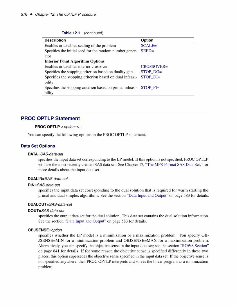
576 F Chapter 12: The OPTLP Procedure
Table 12.1 (continued)
Description OptionEnables or disables scaling of the problem SCALE=Specifies the initial seed for the random number gener-ator
SEED=
Interior Point Algorithm OptionsEnables or disables interior crossover CROSSOVER=Specifies the stopping criterion based on duality gap STOP_DG=Specifies the stopping criterion based on dual infeasi-bility
STOP_DI=
Specifies the stopping criterion based on primal infeasi-bility
STOP_PI=
PROC OPTLP StatementPROC OPTLP < options > ;
You can specify the following options in the PROC OPTLP statement.
Data Set Options
DATA=SAS-data-setspecifies the input data set corresponding to the LP model. If this option is not specified, PROC OPTLPwill use the most recently created SAS data set. See Chapter 17, “The MPS-Format SAS Data Set,” formore details about the input data set.
DUALIN=SAS-data-set
DIN=SAS-data-setspecifies the input data set corresponding to the dual solution that is required for warm starting theprimal and dual simplex algorithms. See the section “Data Input and Output” on page 583 for details.
DUALOUT=SAS-data-set
DOUT=SAS-data-setspecifies the output data set for the dual solution. This data set contains the dual solution information.See the section “Data Input and Output” on page 583 for details.
OBJSENSE=optionspecifies whether the LP model is a minimization or a maximization problem. You specify OB-JSENSE=MIN for a minimization problem and OBJSENSE=MAX for a maximization problem.Alternatively, you can specify the objective sense in the input data set; see the section “ROWS Section”on page 841 for details. If for some reason the objective sense is specified differently in these twoplaces, this option supersedes the objective sense specified in the input data set. If the objective sense isnot specified anywhere, then PROC OPTLP interprets and solves the linear program as a minimizationproblem.

PROC OPTLP Statement F 577
PRIMALIN=SAS-data-set
PIN=SAS-data-setspecifies the input data set corresponding to the primal solution that is required for warm starting theprimal and dual simplex algorithms. See the section “Data Input and Output” on page 583 for details.
PRIMALOUT=SAS-data-set
POUT=SAS-data-setspecifies the output data set for the primal solution. This data set contains the primal solutioninformation. See the section “Data Input and Output” on page 583 for details.
SAVE_ONLY_IF_OPTIMALspecifies that the PRIMALOUT= and DUALOUT= data sets be saved only if the final solution obtainedby the solver at termination is optimal. If the PRIMALOUT= and DUALOUT= options are specified,then by default (that is, omitting the SAVE_ONLY_IF_OPTIMAL option), PROC OPTLP always savesthe solutions obtained at termination, regardless of the final status. If the SAVE_ONLY_IF_OPTIMALoption is not specified, the output data sets can contain an intermediate solution, if one is available.
Solver Options
IIS=number | stringspecifies whether PROC OPTLP attempts to identify a set of constraints and variables that form anirreducible infeasible set (IIS). Table 12.2 describes the valid values of the IIS= option.
Table 12.2 Values for IIS= Option
number string Description0 OFF Disables IIS detection.1 ON Enables IIS detection.
If an IIS is found, information about infeasible constraints or variable bounds can be found in theDUALOUT= and PRIMALOUT= data sets. The default value of this option is OFF. See the section“Irreducible Infeasible Set” on page 597 for details.
ALGORITHM=option
SOLVER=option
SOL=optionspecifies one of the following LP algorithms:
Option DescriptionPRIMAL (PS) Uses primal simplex algorithm.DUAL (DS) Uses dual simplex algorithm.NETWORK (NS) Uses network simplex algorithm.INTERIORPOINT (IP) Uses interior point algorithm.CONCURRENT (CON) Uses several different algorithms
in parallel.
The valid abbreviated value for each option is indicated in parentheses. By default, the dual simplexalgorithm is used.

578 F Chapter 12: The OPTLP Procedure
ALGORITHM2=option
SOLVER2=optionspecifies one of the following LP algorithms if ALGORITHM=NS:
Option DescriptionPRIMAL (PS) Uses primal simplex algorithm (after network sim-
plex).DUAL (DS) Uses dual simplex algorithm (after network simplex).
The valid abbreviated value for each option is indicated in parentheses. By default, the OPTLPprocedure decides which algorithm is best to use after calling the network simplex algorithm on theextracted network.
Presolve Options
PRESOLVER=number | string
PRESOL=number | stringspecifies one of the following presolve options:
number string Description–1 AUTOMATIC Applies presolver by using default settings.0 NONE Disables presolver.1 BASIC Performs basic presolve such as removing empty rows,
columns, and fixed variables.2 MODERATE Performs basic presolve and applies other inexpensive
presolve techniques.3 AGGRESSIVE Performs moderate presolve and applies other aggres-
sive (but expensive) presolve techniques.
The default option is AUTOMATIC (–1), which is somewhere between the MODERATE and AGRES-SIVE setting. See the section “Presolve” on page 587 for details.
DUALIZE=number | stringcontrols the dualization of the problem:
number string Description–1 AUTOMATIC The presolver uses a heuristic to decide whether to
dualize the problem or not.0 OFF Disables dualization. The optimization problem is
solved in the form that you specify.1 ON The presolver formulates the dual of the linear opti-
mization problem.
Dualization is usually helpful for problems that have many more constraints than variables. You canuse this option with all simplex algorithms in PROC OPTLP, but it is most effective with the primaland dual simplex algorithms.

PROC OPTLP Statement F 579
The default option is AUTOMATIC.
Control Options
FEASTOL=�specifies the feasibility tolerance � 2[1E–9, 1E–4] for determining the feasibility of a variable value.The default value is 1E–6.
LOGFREQ=kPRINTFREQ=k
specifies that the printing of the solution progress to the iteration log is to occur after every k iterations.The print frequency, k, is an integer between zero and the largest four-byte signed integer, which is231 � 1.
The value k D 0 disables the printing of the progress of the solution.
If the LOGFREQ= option is not specified, then PROC OPTLP displays the iteration log with a dynamicfrequency according to the problem size if the primal or dual simplex algorithm is used, with frequency10,000 if the network simplex algorithm is used, or with frequency 1 if the interior point algorithm isused.
LOGLEVEL=number | string
PRINTLEVEL2=number | stringcontrols the amount of information displayed in the SAS log by the LP solver, from a short descriptionof presolve information and summary to details at each iteration. Table 12.7 describes the valid valuesfor this option.
Table 12.7 Values for LOGLEVEL= Option
number string Description0 NONE Turn off all solver-related messages in SAS log.1 BASIC Display a solver summary after stopping.2 MODERATE Print a solver summary and an iteration log by
using the interval dictated by the LOGFREQ= op-tion.
3 AGGRESSIVE Print a detailed solver summary and an itera-tion log by using the interval dictated by theLOGFREQ= option.
The default value is MODERATE.
MAXITER=kspecifies the maximum number of iterations. The value k can be any integer between one and thelargest four-byte signed integer, which is 231 � 1. If you do not specify this option, the proceduredoes not stop based on the number of iterations performed. For network simplex, this iteration limitcorresponds to the algorithm called after network simplex (either primal or dual simplex).

580 F Chapter 12: The OPTLP Procedure
MAXTIME=tspecifies an upper limit of t seconds of time for reading in the data and performing the optimizationprocess. The value of the TIMETYPE= option determines the type of units used. If you do not specifythis option, the procedure does not stop based on the amount of time elapsed. The value of t can beany positive number; the default value is the positive number that has the largest absolute value thatcan be represented in your operating environment.
OPTTOL=�specifies the optimality tolerance � 2[1E–9, 1E–4] for declaring optimality. The default value is 1E–6.
PRINTLEVEL=0 j 1 j 2specifies whether a summary of the problem and solution should be printed. If PRINTLEVEL=1, thenthe Output Delivery System (ODS) tables ProblemSummary, SolutionSummary, and PerformanceInfoare produced and printed. If PRINTLEVEL=2, then the same tables are produced and printed alongwith an additional table called ProblemStatistics. If PRINTLEVEL=0, then no ODS tables are producedor printed. The default value is 1.
For details about the ODS tables created by PROC OPTLP, see the section “ODS Tables” on page 594.
TIMETYPE=number | stringspecifies whether CPU time or real time is used for the MAXTIME= option and the _OROPTLP_macro variable in a PROC OPTLP call. Table 12.8 describes the valid values of the TIMETYPE=option.
Table 12.8 Values for TIMETYPE= Option
number string Description0 CPU Specifies units of CPU time.1 REAL Specifies units of real time.
The default value of the TIMETYPE= option depends on the values of the NTHREADS= and NODES=options in the PERFORMANCE statement. For more information about the NTHREADS= andNODES= options, see the section “PERFORMANCE Statement” on page 19 in Chapter 4, “SharedConcepts and Topics.”
If you specify a value greater than 1 for either the NTHREADS= or the NODES= option, the defaultvalue of the TIMETYPE= option is REAL. If you specify a value of 1 for both the NTHREADS= andNODES= options, the default value of the TIMETYPE= option is CPU.
Simplex Algorithm Options
BASIS=number | stringspecifies the following options for generating an initial basis:
number string Description0 CRASH Generate an initial basis by using crash techniques (Maros
2003). The procedure creates a triangular basic matrixconsisting of both decision variables and slack variables.
1 SLACK Generate an initial basis by using all slack variables.

PROC OPTLP Statement F 581
number string Description2 WARMSTART Start the primal and dual simplex algorithms with a user-
specified initial basis. The PRIMALIN= and DUALIN=data sets are required to specify an initial basis.
The default option is determined automatically based on the problem structure. For network simplex,this option has no effect.
PRICETYPE=number | stringspecifies one of the following pricing strategies for the primal and dual simplex algorithms:
number string Description0 HYBRID Use a hybrid of Devex and steepest-edge pricing strate-
gies. Available for the primal simplex algorithm only.1 PARTIAL Use Dantzig’s rule on a queue of decision variables.
Optionally, you can specify QUEUESIZE=. Availablefor the primal simplex algorithm only.
2 FULL Use Dantzig’s rule on all decision variables.3 DEVEX Use Devex pricing strategy.4 STEEPESTEDGE Use steepest-edge pricing strategy.
The default option is determined automatically based on the problem structure. For the network simplexalgorithm, this option applies only to the algorithm specified by the ALGORITHM2= option. See thesection “Pricing Strategies for the Primal and Dual Simplex Algorithms” on page 587 for details.
QUEUESIZE=kspecifies the queue size k 2 Œ1; n�, where n is the number of decision variables. This queue is used forfinding an entering variable in the simplex iteration. The default value is chosen adaptively based onthe number of decision variables. This option is used only when PRICETYPE=PARTIAL.
SCALE=number | stringspecifies one of the following scaling options:
number string Description0 NONE Disable scaling.–1 AUTOMATIC Automatically apply scaling procedure if necessary.
The default option is AUTOMATIC.
SEED=numberspecifies the initial seed for the random number generator. Because the seed affects the perturbationin the simplex algorithms, the result might be a different optimal solution and a different solver path,but the effect is usually negligible. The value of number can be any positive integer up to the largestfour-byte signed integer, which is 231 � 1. By default, SEED=100.

582 F Chapter 12: The OPTLP Procedure
Interior Point Algorithm Options
CROSSOVER=number | stringspecifies whether to convert the interior point solution to a basic simplex solution. If the interior pointalgorithm terminates with a solution, the crossover algorithm uses the interior point solution to createan initial basic solution. After performing primal fixing and dual fixing, the crossover algorithm calls asimplex algorithm to locate an optimal basic solution.
number string Description0 OFF Do not convert the interior point solution to a basic
simplex solution.1 ON Convert the interior point solution to a basic simplex
solution.
The default value of the CROSSOVER= option is ON.
STOP_DG=ıspecifies the desired relative duality gap ı 2[1E–9, 1E–4]. This is the relative difference between theprimal and dual objective function values and is the primary solution quality parameter. The defaultvalue is 1E–6. See the section “The Interior Point Algorithm” on page 589 for details.
STOP_DI=ˇspecifies the maximum allowed relative dual constraints violation ˇ 2[1E–9, 1E–4]. The default valueis 1E–6. See the section “The Interior Point Algorithm” on page 589 for details.
STOP_PI=˛specifies the maximum allowed relative bound and primal constraints violation ˛ 2[1E–9, 1E–4]. Thedefault value is 1E–6. See the section “The Interior Point Algorithm” on page 589 for details.
Decomposition Algorithm StatementsThe following statements are available for the decomposition algorithm in the OPTLP procedure:
DECOMP < options > ;
DECOMP_MASTER < options > ;
DECOMP_SUBPROB < options > ;
For more information about these statements, see Chapter 15, “The Decomposition Algorithm.”
PERFORMANCE StatementPERFORMANCE < performance-options > ;
The PERFORMANCE statement specifies performance-options for single-machine mode and distributedmode, and requests detailed performance results of the OPTLP procedure.

Details: OPTLP Procedure F 583
You can also use the PERFORMANCE statement to control whether the OPTLP procedure executes insingle-machine or distributed mode. The PERFORMANCE statement is documented in the section “PER-FORMANCE Statement” on page 19 in Chapter 4, “Shared Concepts and Topics.”
For the OPTLP procedure, the decomposition algorithm, interior point algorithm, and concurrent LP algorithmcan be run in single-machine mode. Only the decomposition algorithm can be run in distributed mode. Thedecomposition algorithm and concurrent LP algorithm support both the deterministic and nondeterministicmodes. The interior point algorithm supports only the deterministic mode.
NOTE: Distributed mode requires SAS High-Performance Optimization.
Details: OPTLP Procedure
Data Input and OutputThis subsection describes the PRIMALIN= and DUALIN= data sets required to warm start the primal anddual simplex algorithms, and the PRIMALOUT= and DUALOUT= output data sets.
Definitions of Variables in the PRIMALIN= Data Set
The PRIMALIN= data set has two required variables defined as follows:
_VAR_specifies the name of the decision variable.
_STATUS_specifies the status of the decision variable. It can take one of the following values:
B basic variable
L nonbasic variable at its lower bound
U nonbasic variable at its upper bound
F free variable
A newly added variable in the modified LP model when using the BASIS=WARMSTART option
NOTE: The PRIMALIN= data set is created from the PRIMALOUT= data set that is obtained from aprevious “normal” run of PROC OPTLP (one that uses only the DATA= data set as the input).
Definitions of Variables in the DUALIN= Data Set
The DUALIN= data set also has two required variables defined as follows:
_ROW_specifies the name of the constraint.

584 F Chapter 12: The OPTLP Procedure
_STATUS_specifies the status of the slack variable for a given constraint. It can take one of the following values:
B basic variable
L nonbasic variable at its lower bound
U nonbasic variable at its upper bound
F free variable
A newly added variable in the modified LP model when using the BASIS=WARMSTART option
NOTE: The DUALIN= data set is created from the DUALOUT= data set that is obtained from a previous“normal” run of PROC OPTLP (one that uses only the DATA= data set as the input).
Definitions of Variables in the PRIMALOUT= Data Set
The PRIMALOUT= data set contains the primal solution to the LP model; each observation corresponds to avariable of the LP problem. If the SAVE_ONLY_IF_OPTIMAL option is not specified, the PRIMALOUT=data set can contain an intermediate solution, if one is available. See Example 12.1 for an example of thePRIMALOUT= data set. The variables in the data set have the following names and meanings.
_OBJ_ID_specifies the name of the objective function. This is particularly useful when there are multipleobjective functions, in which case each objective function has a unique name.
NOTE: PROC OPTLP does not support simultaneous optimization of multiple objective functions inthis release.
_RHS_ID_specifies the name of the variable that contains the right-hand-side value of each constraint.
_VAR_specifies the name of the decision variable.
_TYPE_specifies the type of the decision variable. _TYPE_ can take one of the following values:
N nonnegative
D bounded (with both lower and upper bound)
F free
X fixed
O other (with either lower or upper bound)
_OBJCOEF_specifies the coefficient of the decision variable in the objective function.
_LBOUND_specifies the lower bound on the decision variable.
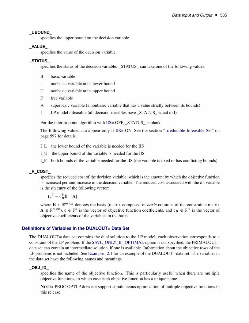
Data Input and Output F 585
_UBOUND_specifies the upper bound on the decision variable.
_VALUE_specifies the value of the decision variable.
_STATUS_specifies the status of the decision variable. _STATUS_ can take one of the following values:
B basic variable
L nonbasic variable at its lower bound
U nonbasic variable at its upper bound
F free variable
A superbasic variable (a nonbasic variable that has a value strictly between its bounds)
I LP model infeasible (all decision variables have _STATUS_ equal to I)
For the interior point algorithm with IIS= OFF, _STATUS_ is blank.
The following values can appear only if IIS= ON. See the section “Irreducible Infeasible Set” onpage 597 for details.
I_L the lower bound of the variable is needed for the IIS
I_U the upper bound of the variable is needed for the IIS
I_F both bounds of the variable needed for the IIS (the variable is fixed or has conflicting bounds)
_R_COST_specifies the reduced cost of the decision variable, which is the amount by which the objective functionis increased per unit increase in the decision variable. The reduced cost associated with the ith variableis the ith entry of the following vector:�
cT� cT
BB�1A�
where B 2 Rm�m denotes the basis (matrix composed of basic columns of the constraints matrixA 2 Rm�n), c 2 Rn is the vector of objective function coefficients, and cB 2 Rm is the vector ofobjective coefficients of the variables in the basis.
Definitions of Variables in the DUALOUT= Data Set
The DUALOUT= data set contains the dual solution to the LP model; each observation corresponds to aconstraint of the LP problem. If the SAVE_ONLY_IF_OPTIMAL option is not specified, the PRIMALOUT=data set can contain an intermediate solution, if one is available. Information about the objective rows of theLP problems is not included. See Example 12.1 for an example of the DUALOUT= data set. The variables inthe data set have the following names and meanings.
_OBJ_ID_specifies the name of the objective function. This is particularly useful when there are multipleobjective functions, in which case each objective function has a unique name.
NOTE: PROC OPTLP does not support simultaneous optimization of multiple objective functions inthis release.

586 F Chapter 12: The OPTLP Procedure
_RHS_ID_specifies the name of the variable that contains the right-hand-side value of each constraint.
_ROW_specifies the name of the constraint.
_TYPE_specifies the type of the constraint. _TYPE_ can take one of the following values:
L “less than or equals” constraint
E equality constraint
G “greater than or equals” constraint
R ranged constraint (both “less than or equals” and “greater than or equals”)
_RHS_specifies the value of the right-hand side of the constraint. It takes a missing value for a rangedconstraint.
_L_RHS_specifies the lower bound of a ranged constraint. It takes a missing value for a non-ranged constraint.
_U_RHS_specifies the upper bound of a ranged constraint. It takes a missing value for a non-ranged constraint.
_VALUE_specifies the value of the dual variable associated with the constraint.
_STATUS_specifies the status of the slack variable for the constraint. _STATUS_ can take one of the followingvalues:
B basic variable
L nonbasic variable at its lower bound
U nonbasic variable at its upper bound
F free variable
A superbasic variable (a nonbasic variable that has a value strictly between its bounds)
I LP model infeasible (all decision variables have _STATUS_ equal to I)
The following values can appear only if option IIS= ON. See the section “Irreducible Infeasible Set”on page 597 for details.
I_L the “GE” (�) condition of the constraint is needed for the IIS
I_U the “LE” (�) condition of the constraint is needed for the IIS
I_F both conditions of the constraint are needed for the IIS (the constraint is an equality or a rangeconstraint with conflicting bounds)

Presolve F 587
_ACTIVITY_specifies the left-hand-side value of a constraint. In other words, the value of _ACTIVITY_ for the ithconstraint would be equal to aT
i x, where ai refers to the ith row of the constraints matrix and x denotesthe vector of current decision variable values.
PresolvePresolve in PROC OPTLP uses a variety of techniques to reduce the problem size, improve numerical stability,and detect infeasibility or unboundedness (Andersen and Andersen 1995; Gondzio 1997). During presolve,redundant constraints and variables are identified and removed. Presolve can further reduce the problemsize by substituting variables. Variable substitution is a very effective technique, but it might occasionallyincrease the number of nonzero entries in the constraint matrix.
In most cases, using presolve is very helpful in reducing solution times. You can enable presolve at differentlevels or disable it by specifying the PRESOLVER= option.
Pricing Strategies for the Primal and Dual Simplex AlgorithmsSeveral pricing strategies for the primal and dual simplex algorithms are available. Pricing strategiesdetermine which variable enters the basis at each simplex pivot. They can be controlled by specifying thePRICETYPE= option.
The primal simplex algorithm has the following five pricing strategies:
PARTIAL uses Dantzig’s most violated reduced cost rule (Dantzig 1963). It scans a queue ofdecision variables and selects the variable with the most violated reduced cost as theentering variable. You can optionally specify the QUEUESIZE= option to control thelength of this queue.
FULL uses Dantzig’s most violated reduced cost rule. It compares the reduced costs of alldecision variables and selects the variable with the most violated reduced cost as theentering variable.
DEVEX implements the Devex pricing strategy developed by Harris (1973).
STEEPESTEDGE uses the steepest-edge pricing strategy developed by Forrest and Goldfarb (1992).
HYBRID uses a hybrid of the Devex and steepest-edge pricing strategies.
The dual simplex algorithm has only three pricing strategies available: FULL, DEVEX, and STEEPEST-EDGE.
Warm Start for the Primal and Dual Simplex AlgorithmsYou can warm start the primal and dual simplex algorithms by specifying the option BASIS=WARMSTART.Additionally you need to specify the PRIMALIN= and DUALIN= data sets. The primal and dual simplexalgorithms start with the basis thus provided. If the given basis cannot form a valid basis, the algorithms usethe basis generated using their crash techniques.
588 F Chapter 12: The OPTLP Procedure
After an LP model is solved using the primal and dual simplex algorithms, the BASIS=WARMSTART optionenables you to perform sensitivity analysis such as modifying the objective function, changing the right-handsides of the constraints, adding or deleting constraints or decision variables, and combinations of these cases.A faster solution to such a modified LP model can be obtained by starting with the basis in the optimalsolution to the original LP model. This can be done by using the BASIS=WARMSTART option, modifyingthe DATA= input data set, and specifying the PRIMALIN= and DUALIN= data sets. Example 12.4 andExample 12.5 illustrate how to reoptimize an LP problem with a modified objective function and a modifiedright-hand side by using this technique. Example 12.6 shows how to reoptimize an LP problem after addinga new constraint.
The network simplex algorithm ignores the option BASIS=WARMSTART.
CAUTION: Since the presolver uses the objective function and/or right-hand-side information, the basisprovided by you might not be valid for the presolved model. It is therefore recommended that you turn thePRESOLVER= option off when using BASIS=WARMSTART.
The Network Simplex AlgorithmThe network simplex algorithm in PROC OPTLP attempts to leverage the speed of the network simplexalgorithm to more efficiently solve linear programs by using the following process:
1. It heuristically extracts the largest possible network substructure from the original problem.
2. It uses the network simplex algorithm to solve for an optimal solution to this substructure.
3. It uses this solution to construct an advanced basis to warm-start either the primal or dual simplexalgorithm on the original linear programming problem.
The network simplex algorithm is a specialized version of the simplex algorithm that uses spanning-treebases to more efficiently solve linear programming problems that have a pure network form. Such LPs canbe modeled using a formulation over a directed graph, as a minimum-cost flow problem. Let G D .N;A/ bea directed graph, where N denotes the nodes and A denotes the arcs of the graph. The decision variable xij
denotes the amount of flow sent from node i to node j. The cost per unit of flow on the arcs is designated bycij , and the amount of flow sent across each arc is bounded to be within Œlij ; uij �. The demand (or supply) ateach node is designated as bi , where bi > 0 denotes a supply node and bi < 0 denotes a demand node. Thecorresponding linear programming problem is as follows:
minP
.i;j /2A cijxij
subject toP
.i;j /2A xij �P
.j;i/2A xj i D bi 8i 2 N
xij � uij 8.i; j / 2 A
xij � lij 8.i; j / 2 A
The network simplex algorithm used in PROC OPTLP is the primal network simplex algorithm. Thisalgorithm finds the optimal primal feasible solution and a dual solution that satisfies complementary slackness.Sometimes the directed graph G is disconnected. In this case, the problem can be decomposed into its weaklyconnected components and each minimum-cost flow problem can be solved separately. After solving eachcomponent, the optimal basis for the network substructure is augmented with the non-network variables andconstraints from the original problem. This advanced basis is then used as a starting point for the primal or

The Interior Point Algorithm F 589
dual simplex method. The solver automatically selects the algorithm to use after network simplex. However,you can override this selection with the ALGORITHM2= option.
The network simplex algorithm can be more efficient than the other algorithms on problems with a largenetwork substructure. You can view the size of the network structure in the log.
The Interior Point AlgorithmThe interior point algorithm in PROC OPTLP implements an infeasible primal-dual predictor-correctorinterior point algorithm. To illustrate the algorithm and the concepts of duality and dual infeasibility, considerthe following LP formulation (the primal):
min cTxsubject to Ax � b
x � 0
The corresponding dual formulation is as follows:
max bTysubject to ATy C w D c
y � 0w � 0
where y 2 Rm refers to the vector of dual variables and w 2 Rn refers to the vector of dual slack variables.
The dual formulation makes an important contribution to the certificate of optimality for the primal formu-lation. The primal and dual constraints combined with complementarity conditions define the first-orderoptimality conditions, also known as KKT (Karush-Kuhn-Tucker) conditions, which can be stated as follows:
Ax � s D b .primal feasibility/ATyC w D c .dual feasibility/
WXe D 0 .complementarity/SYe D 0 .complementarity/
x; y; w; s � 0
where e � .1; : : : ; 1/T of appropriate dimension and s 2 Rm is the vector of primal slack variables.
NOTE: Slack variables (the s vector) are automatically introduced by the algorithm when necessary; it istherefore recommended that you not introduce any slack variables explicitly. This enables the algorithm tohandle slack variables much more efficiently.
The letters X; Y;W; and S denote matrices with corresponding x, y, w, and s on the main diagonal and zeroelsewhere, as in the following example:
X �
26664x1 0 � � � 0
0 x2 � � � 0:::
:::: : :
:::
0 0 � � � xn
37775
590 F Chapter 12: The OPTLP Procedure
If .x�; y�;w�; s�/ is a solution of the previously defined system of equations that represent the KKTconditions, then x� is also an optimal solution to the original LP model.
At each iteration the interior point algorithm solves a large, sparse system of linear equations,�Y�1S AAT �X�1W
� ��y�x
�D
�„
‚
�where �x and �y denote the vector of search directions in the primal and dual spaces, respectively, and ‚and „ constitute the vector of the right-hand sides.
The preceding system is known as the reduced KKT system. PROC OPTLP uses a preconditioned quasi-minimum residual algorithm to solve this system of equations efficiently.
An important feature of the interior point algorithm is that it takes full advantage of the sparsity in theconstraint matrix, thereby enabling it to efficiently solve large-scale linear programs.
The interior point algorithm works simultaneously in the primal and dual spaces. It attains optimality whenboth primal and dual feasibility are achieved and when complementarity conditions hold. Therefore, it is ofinterest to observe the following four measures where kvk2 is the Euclidean norm of the vector v:
� relative primal infeasibility measure ˛:
˛ DkAx � b � sk2kbk2 C 1
� relative dual infeasibility measure ˇ:
ˇ Dkc �ATy � wk2kck2 C 1
� relative duality gap ı:
ı DjcTx � bTyjjcTxj C 1
� absolute complementarity :
D
nXiD1
xiwi C
mXiD1
yisi
These measures are displayed in the iteration log.
Iteration Log for the Primal and Dual Simplex AlgorithmsThe primal and dual simplex algorithms implement a two-phase simplex algorithm. Phase I finds a feasiblesolution, which phase II improves to an optimal solution.
When LOGFREQ=1, the following information is printed in the iteration log:

Iteration Log for the Network Simplex Algorithm F 591
Algorithm indicates which simplex method is running by printing the letter P (primal) or D (dual).
Phase indicates whether the algorithm is in phase I or phase II of the simplex method.
Iteration indicates the iteration number.
Objective Value indicates the current amount of infeasibility in phase I and the primal objective value ofthe current solution in phase II.
Time indicates the time elapsed (in seconds).
Entering Variable indicates the entering pivot variable. A slack variable that enters the basis is indicatedby the corresponding row name followed by “(S)”. If the entering nonbasic variablehas distinct and finite lower and upper bounds, then a “bound swap” can take place inthe primal simplex method.
Leaving Variable indicates the leaving pivot variable. A slack variable that leaves the basis is indicatedby the corresponding row name followed by “(S)”. The leaving variable is the same asthe entering variable if a bound swap has taken place.
When you omit the LOGFREQ= option or specify a value greater than 1, only the algorithm, phase, iteration,objective value, and time information is printed in the iteration log.
The behavior of objective values in the iteration log depends on both the current phase and the chosenalgorithm. In phase I, both simplex methods have artificial objective values that decrease to 0 when afeasible solution is found. For the dual simplex method, phase II maintains a dual feasible solution, so aminimization problem has increasing objective values in the iteration log. For the primal simplex method,phase II maintains a primal feasible solution, so a minimization problem has decreasing objective values inthe iteration log.
During the solution process, some elements of the LP model might be perturbed to improve performance. Inthis case the objective values that are printed correspond to the perturbed problem. After reaching optimalityfor the perturbed problem, PROC OPTLP solves the original problem by switching from the primal simplexmethod to the dual simplex method (or from the dual to the primal simplex method). Because the problemmight be perturbed again, this process can result in several changes between the two algorithms.
Iteration Log for the Network Simplex AlgorithmAfter finding the embedded network and formulating the appropriate relaxation, the network simplexalgorithm uses a primal network simplex algorithm. In the case of a connected network, with one (weaklyconnected) component, the log shows the progress of the simplex algorithm. The following information isdisplayed in the iteration log:
Iteration indicates the iteration number.
PrimalObj indicates the primal objective value of the current solution.
Primal Infeas indicates the maximum primal infeasibility of the current solution.
Time indicates the time spent on the current component by network simplex.
The frequency of the simplex iteration log is controlled by the LOGFREQ= option. The default value of theLOGFREQ= option is 10,000.

592 F Chapter 12: The OPTLP Procedure
If the network relaxation is disconnected, the information in the iteration log shows progress at the componentlevel. The following information is displayed in the iteration log:
Component indicates the component number being processed.
Nodes indicates the number of nodes in this component.
Arcs indicates the number of arcs in this component.
Iterations indicates the number of simplex iterations needed to solve this component.
Time indicates the time spent so far in network simplex.
The frequency of the component iteration log is controlled by the LOGFREQ= option. In this case, thedefault value of the LOGFREQ= option is determined by the size of the network.
The LOGLEVEL= option adjusts the amount of detail shown. By default, LOGLEVEL= is set to MODER-ATE and reports as described previously. If set to NONE, no information is shown. If set to BASIC, the onlyinformation shown is a summary of the network relaxation and the time spent solving the relaxation. If setto AGGRESSIVE, in the case of one component, the log displays as described previously; in the case ofmultiple components, for each component, a separate simplex iteration log is displayed.
Iteration Log for the Interior Point AlgorithmThe interior point algorithm implements an infeasible primal-dual predictor-corrector interior point algorithm.The following information is displayed in the iteration log:
Iter indicates the iteration number.
Complement indicates the (absolute) complementarity.
Duality Gap indicates the (relative) duality gap.
Primal Infeas indicates the (relative) primal infeasibility measure.
Bound Infeas indicates the (relative) bound infeasibility measure.
Dual Infeas indicates the (relative) dual infeasibility measure.
Time indicates the time elapsed (in seconds).
If the sequence of solutions converges to an optimal solution of the problem, you should see all columnsin the iteration log converge to zero or very close to zero. If they do not, it can be the result of insufficientiterations being performed to reach optimality. In this case, you might need to increase the value specified inthe MAXITER= or MAXTIME= options. If the complementarity or the duality gap do not converge, theproblem might be infeasible or unbounded. If the infeasibility columns do not converge, the problem mightbe infeasible.
Iteration Log for the Crossover AlgorithmThe crossover algorithm takes an optimal solution from the interior point algorithm and transforms it intoan optimal basic solution. The iterations of the crossover algorithm are similar to simplex iterations; thissimilarity is reflected in the format of the iteration logs.

Concurrent LP F 593
When LOGFREQ=1, the following information is printed in the iteration log:
Phase indicates whether the primal crossover (PC) or dual crossover (DC) technique is used.
Iteration indicates the iteration number.
Objective Value indicates the total amount by which the superbasic variables are off their bound. Thisvalue decreases to 0 as the crossover algorithm progresses.
Time indicates the time elapsed (in seconds).
Entering Variable indicates the entering pivot variable. A slack variable that enters the basis is indicatedby the corresponding row name followed by “(S).”
Leaving Variable indicates the leaving pivot variable. A slack variable that leaves the basis is indicated bythe corresponding row name followed by “(S).”
When you omit the LOGFREQ= option or specify a value greater than 1, only the phase, iteration, objectivevalue, and time information is printed in the iteration log.
After all the superbasic variables have been eliminated, the crossover algorithm continues with regular primalor dual simplex iterations.
Concurrent LPThe ALGORITHM=CON option starts several different linear optimization algorithms in parallel in asingle-machine mode. The OPTLP procedure automatically determines which algorithms to run and howmany threads to assign to each algorithm. If sufficient resources are available, the procedure runs all fourstandard algorithms. When the first algorithm ends, the procedure returns the results from that algorithmand terminates any other algorithms that are still running. If you specify a value of DETERMINISTIC forthe PARALLELMODE= option in the PERFORMANCE statement, the algorithm for which the results arereturned is not necessarily the one that finished first. The OPTLP procedure deterministically selects thealgorithm for which the results are returned. Regardless of which mode (deterministic or nondeterministic) isin effect, terminating algorithms that are still running might take a significant amount of time.
During concurrent optimization, the procedure displays the iteration log for the dual simplex algorithm. Formore information about this iteration log, see the section “Iteration Log for the Primal and Dual SimplexAlgorithms” on page 590. Upon termination, the procedure displays the iteration log for the algorithm thatfinishes first, unless the dual simplex algorithm finishes first. If you specify LOGLEVEL=AGGRESSIVE,the OPTLP procedure displays the iteration logs for all algorithms that are run concurrently.
If you specify PRINTLEVEL=2 and ALGORITHM=CON, the OPTLP procedure produces an ODS tablecalled ConcurrentSummary. This table contains a summary of the solution statuses of all algorithms that arerun concurrently.
Parallel ProcessingThe interior point and concurrent LP algorithms can be run in single-machine mode (in single-machine mode,the computation is executed by multiple threads on a single computer). The decomposition algorithm can

594 F Chapter 12: The OPTLP Procedure
be run in either single-machine or distributed mode (in distributed mode, the computation is executed onmultiple computing nodes in a distributed computing environment).
NOTE: Distributed mode requires SAS High-Performance Optimization.
You can specify options for parallel processing in the PERFORMANCE statement, which is documented inthe section “PERFORMANCE Statement” on page 19 in Chapter 4, “Shared Concepts and Topics.”
ODS TablesPROC OPTLP creates three Output Delivery System (ODS) tables by default. The first table, ProblemSum-mary, is a summary of the input LP problem. The second table, SolutionSummary, is a brief summary of thesolution status. The third table, PerformanceInfo, is a summary of performance options. You can use ODStable names to select tables and create output data sets. For more information about ODS, see SAS OutputDelivery System: Procedures Guide.
If you specify a value of 2 for the PRINTLEVEL= option, then the ProblemStatistics table is produced. Thistable contains information about the problem data. For more information, see the section “Problem Statistics”on page 596. If you specify PRINTLEVEL=2 and ALGORITHM=CON, the ConcurrentSummary table isproduced. This table contains solution status information for all algorithms that are run concurrently. Formore information, see the section “Concurrent LP” on page 593.
If you specify the DETAILS option in the PERFORMANCE statement, then the Timing table is produced.
Table 12.13 lists all the ODS tables that can be produced by the OPTLP procedure, along with the statementand option specifications required to produce each table.
Table 12.13 ODS Tables Produced by PROC OPTLP
ODS Table Name Description Statement OptionProblemSummary Summary of the input LP problem PROC OPTLP PRINTLEVEL=1
(default)SolutionSummary Summary of the solution status PROC OPTLP PRINTLEVEL=1
(default)ProblemStatistics Description of input problem data PROC OPTLP PRINTLEVEL=2ConcurrentSummary Summary of the solution status for
all algorithms run concurrentlyPROC OPTLP PRINTLEVEL=2,
ALGORITHM=CONPerformanceInfo List of performance options and
their valuesPROC OPTLP PRINTLEVEL=1
(default)Timing Detailed solution timing PERFORMANCE DETAILS
A typical output of PROC OPTLP is shown in Figure 12.2.

ODS Tables F 595
Figure 12.2 Typical OPTLP Output
The OPTLP ProcedureThe OPTLP Procedure
Problem Summary
Problem Name ADLITTLE
Objective Sense Minimization
Objective Function .Z....
RHS ZZZZ0001
Number of Variables 97
Bounded Above 0
Bounded Below 97
Bounded Above and Below 0
Free 0
Fixed 0
Number of Constraints 56
LE (<=) 40
EQ (=) 15
GE (>=) 1
Range 0
Constraint Coefficients 383
Performance Information
Execution Mode Single-Machine
Number of Threads 4
Solution Summary
Solver LP
Algorithm Dual Simplex
Objective Function .Z....
Solution Status Optimal
Objective Value 225494.96316
Primal Infeasibility 2.273737E-13
Dual Infeasibility 5.684342E-14
Bound Infeasibility 0
Iterations 74
Presolve Time 0.00
Solution Time 0.02
You can create output data sets from these tables by using the ODS OUTPUT statement. This can be useful,for example, when you want to create a report to summarize multiple PROC OPTLP runs. The output datasets corresponding to the preceding output are shown in Figure 12.3, where you can also find (at the rowfollowing the heading of each data set in display) the variable names that are used in the table definition(template) of each table.
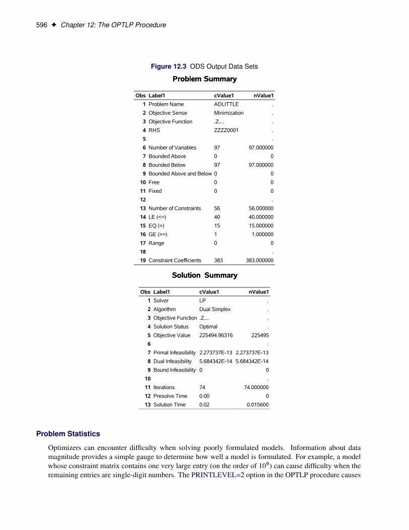
596 F Chapter 12: The OPTLP Procedure
Figure 12.3 ODS Output Data Sets
Problem SummaryProblem Summary
Obs Label1 cValue1 nValue1
1 Problem Name ADLITTLE .
2 Objective Sense Minimization .
3 Objective Function .Z.... .
4 RHS ZZZZ0001 .
5 .
6 Number of Variables 97 97.000000
7 Bounded Above 0 0
8 Bounded Below 97 97.000000
9 Bounded Above and Below 0 0
10 Free 0 0
11 Fixed 0 0
12 .
13 Number of Constraints 56 56.000000
14 LE (<=) 40 40.000000
15 EQ (=) 15 15.000000
16 GE (>=) 1 1.000000
17 Range 0 0
18 .
19 Constraint Coefficients 383 383.000000
Solution SummarySolution Summary
Obs Label1 cValue1 nValue1
1 Solver LP .
2 Algorithm Dual Simplex .
3 Objective Function .Z.... .
4 Solution Status Optimal .
5 Objective Value 225494.96316 225495
6 .
7 Primal Infeasibility 2.273737E-13 2.273737E-13
8 Dual Infeasibility 5.684342E-14 5.684342E-14
9 Bound Infeasibility 0 0
10 .
11 Iterations 74 74.000000
12 Presolve Time 0.00 0
13 Solution Time 0.02 0.015600
Problem Statistics
Optimizers can encounter difficulty when solving poorly formulated models. Information about datamagnitude provides a simple gauge to determine how well a model is formulated. For example, a modelwhose constraint matrix contains one very large entry (on the order of 109) can cause difficulty when theremaining entries are single-digit numbers. The PRINTLEVEL=2 option in the OPTLP procedure causes

Irreducible Infeasible Set F 597
the ODS table ProblemStatistics to be generated. This table provides basic data magnitude information thatenables you to improve the formulation of your models.
The example output in Figure 12.4 demonstrates the contents of the ODS table ProblemStatistics.
Figure 12.4 ODS Table ProblemStatistics
The OPTLP ProcedureThe OPTLP Procedure
Problem Statistics
Number of Constraint Matrix Nonzeros 8
Maximum Constraint Matrix Coefficient 3
Minimum Constraint Matrix Coefficient 1
Average Constraint Matrix Coefficient 1.875
Number of Objective Nonzeros 3
Maximum Objective Coefficient 4
Minimum Objective Coefficient 2
Average Objective Coefficient 3
Number of RHS Nonzeros 3
Maximum RHS 7
Minimum RHS 4
Average RHS 5.3333333333
Maximum Number of Nonzeros per Column 3
Minimum Number of Nonzeros per Column 2
Average Number of Nonzeros per Column 2.67
Maximum Number of Nonzeros per Row 3
Minimum Number of Nonzeros per Row 2
Average Number of Nonzeros per Row 2.67
Irreducible Infeasible SetFor a linear programming problem, an irreducible infeasible set (IIS) is an infeasible subset of constraints andvariable bounds that will become feasible if any single constraint or variable bound is removed. It is possibleto have more than one IIS in an infeasible LP. Identifying an IIS can help isolate the structural infeasibility inan LP.
The presolver in the OPTLP procedure can detect infeasibility, but it identifies only the variable bound orconstraint that triggers the infeasibility.

598 F Chapter 12: The OPTLP Procedure
The IIS=ON option directs the OPTLP procedure to search for an IIS in a specified LP. The OPTLP proceduredoes not apply the presolver to the problem during the IIS search. If PROC OPTLP detects an IIS, it firstoutputs the IIS to the data sets that are specified by the PRIMALOUT= and DUALOUT= options, and thenit stops. The number of iterations that are reported in the macro variable and the ODS table is the totalnumber of simplex iterations. This total includes the initial LP solve and all subsequent iterations during theconstraint deletion phase.
The IIS= option can add special values to the _STATUS_ variables in the output data sets. (For moreinformation, see the section “Data Input and Output” on page 583.) For constraints, a status of “I_L”, “I_U”,or “I_F” indicates that the “GE” (�), “LE” (�), or “EQ” (=) constraint, respectively, is part of the IIS.For range constraints, a status of “I_L” or “I_U” indicates that the lower or upper bound of the constraint,respectively, is needed for the IIS, and “I_F” indicates that the bounds in the constraint are conflicting. Forvariables, a status of “I_L”, “I_U”, or “I_F” indicates that the lower, upper, or both bounds of the variable,respectively, are needed for the IIS. From this information, you can identify both the names of the constraints(variables) in the IIS and the corresponding bound where infeasibility occurs.
Making any one of the constraints or variable bounds in the IIS nonbinding removes the infeasibility fromthe IIS. In some cases, changing a right-hand side or bound by a finite amount removes the infeasibility.However, the only way to guarantee removal of the infeasibility is to set the appropriate right-hand side orbound to1 or �1. Because it is possible for an LP to have multiple irreducible infeasible sets, simplyremoving the infeasibility from one set might not make the entire problem feasible. To make the entireproblem feasible, you can specify IIS=ON and rerun PROC OPTLP after removing the infeasibility from anIIS. Repeating this process until the LP solver no longer detects an IIS results in a feasible problem. Thisapproach to infeasibility repair can produce different end problems depending on which right-hand sides andbounds you choose to relax.
Changing different constraints and bounds can require considerably different changes to the MPS-formatSAS data set. For example, if you use the default lower bound of 0 for a variable but you want to relax thelower bound to �1, you might need to add an MI row to the BOUNDS section of the data set. For moreinformation about changing variable and constraint bounds, see Chapter 17, “The MPS-Format SAS DataSet.”
The IIS= option in PROC OPTLP uses two different methods to identify an IIS:
1. Based on the result of the initial solve, the sensitivity filter removes several constraints and variablebounds immediately while still maintaining infeasibility. This phase is quick and dramatically reducesthe size of the IIS.
2. Next, the deletion filter removes each remaining constraint and variable bound one by one to checkwhich of them are needed to obtain an infeasible system. This second phase is more time consuming,but it ensures that the IIS set that PROC OPTLP returns is indeed irreducible. The progress of thedeletion filter is reported at regular intervals. Occasionally, the sensitivity filter might be called againduring the deletion filter to improve performance.
See Example 12.7 for an example that demonstrates the use of the IIS= option in locating and removinginfeasibilities. You can find more details about IIS algorithms in Chinneck (2008).

Macro Variable _OROPTLP_ F 599
Macro Variable _OROPTLP_The OPTLP procedure defines a macro variable named _OROPTLP_. This variable contains a characterstring that indicates the status of the OPTLP procedure upon termination. The various terms of the variableare interpreted as follows.
STATUSindicates the solver status at termination. It can take one of the following values:
OK The procedure terminated normally.
SYNTAX_ERROR Incorrect syntax was used.
DATA_ERROR The input data were inconsistent.
OUT_OF_MEMORY Insufficient memory was allocated to the procedure.
IO_ERROR A problem occurred in reading or writing data.
ERROR The status cannot be classified into any of the preceding categories.
ALGORITHMindicates the algorithm that produces the solution data in the macro variable. This term appears onlywhen STATUS=OK. It can take one of the following values:
PS The primal simplex algorithm produced the solution data.
DS The dual simplex algorithm produced the solution data.
NS The network simplex algorithm produced the solution data.
IP The interior point algorithm produced the solution data.
DECOMP The decomposition algorithm produced the solution data.
When you run algorithms concurrently (ALGORITHM=CON), this term indicates which algorithm isthe first to terminate.
SOLUTION_STATUSindicates the solution status at termination. It can take one of the following values:
OPTIMAL The solution is optimal.
CONDITIONAL_OPTIMAL The solution is optimal, but some infeasibilities (primal, dualor bound) exceed tolerances due to scaling or preprocessing.
FEASIBLE The problem is feasible.
INFEASIBLE The problem is infeasible.
UNBOUNDED The problem is unbounded.
INFEASIBLE_OR_UNBOUNDED The problem is infeasible or unbounded.
ITERATION_LIMIT_REACHED The maximum allowable number of iterations was reached.
TIME_LIMIT_REACHED The solver reached its execution time limit.
ABORTED The solver was interrupted externally.
FAILED The solver failed to converge, possibly due to numerical issues.

600 F Chapter 12: The OPTLP Procedure
OBJECTIVEindicates the objective value obtained by the solver at termination.
PRIMAL_INFEASIBILITYindicates, for the primal simplex and dual simplex algorithms, the maximum (absolute) violation ofthe primal constraints by the primal solution. For the interior point algorithm, this term indicates therelative violation of the primal constraints by the primal solution.
DUAL_INFEASIBILITYindicates, for the primal simplex and dual simplex algorithms, the maximum (absolute) violation of thedual constraints by the dual solution. For the interior point algorithm, this term indicates the relativeviolation of the dual constraints by the dual solution.
BOUND_INFEASIBILITYindicates, for the primal simplex and dual simplex algorithms, the maximum (absolute) violation ofthe lower or upper bounds (or both) by the primal solution. For the interior point algorithm, this termindicates the relative violation of the lower or upper bounds (or both) by the primal solution.
DUALITY_GAPindicates the (relative) duality gap. This term appears only if the interior point algorithm is used.
COMPLEMENTARITYindicates the (absolute) complementarity. This term appears only if the interior point algorithm is used.
ITERATIONSindicates the number of iterations taken to solve the problem. When the network simplex algorithm isused, this term indicates the number of network simplex iterations taken to solve the network relaxation.When crossover is enabled, this term indicates the number of interior point iterations taken to solve theproblem.
ITERATIONS2indicates the number of simplex iterations performed by the secondary algorithm. In network simplex,the secondary algorithm is selected automatically, unless a value has been specified for the ALGO-RITHM2= option. When crossover is enabled, the secondary algorithm is selected automatically. Thisterm appears only if the network simplex algorithm is used or if crossover is enabled.
PRESOLVE_TIMEindicates the time (in seconds) used in preprocessing.
SOLUTION_TIMEindicates the time (in seconds) taken to solve the problem, including preprocessing time.
NOTE: The time reported in PRESOLVE_TIME and SOLUTION_TIME is either CPU time or real time.The type is determined by the TIMETYPE= option.
When SOLUTION_STATUS has a value of OPTIMAL, CONDITIONAL_OPTIMAL, ITERA-TION_LIMIT_REACHED, or TIME_LIMIT_REACHED, all terms of the _OROPTLP_ macro variable arepresent; for other values of SOLUTION_STATUS, some terms do not appear.

Examples: OPTLP Procedure F 601
Examples: OPTLP Procedure
Example 12.1: Oil Refinery ProblemConsider an oil refinery scenario. A step in refining crude oil into finished oil products involves a distillationprocess that splits crude into various streams. Suppose there are three types of crude available: Arabian light(a_l), Arabian heavy (a_h), and Brega (br). These crudes are distilled into light naphtha (na_l), intermediatenaphtha (na_i), and heating oil (h_o). These in turn are blended into two types of jet fuel. Jet fuel j_1 is madeup of 30% intermediate naphtha and 70% heating oil, and jet fuel j_2 is made up of 20% light naphtha and80% heating oil. What amounts of the three crudes maximize the profit from producing jet fuel (j_1, j_2)?This problem can be formulated as the following linear program:
max �175a_l � 165a_h � 205br C 350j_1 C 350j_2
subject to
.napha_l/ 0:035 a_l C 0:03 a_h C 0:045 br D na_l
.napha_i/ 0:1 a_l C 0:075 a_h C 0:135 br D na_i
.htg_oil/ 0:39 a_l C 0:3 a_h C 0:43 br D h_o
.blend1/ 0:3 j_1 � na_i
.blend2/ 0:2 j_2 � na_l
.blend3/ 0:7 j_1 C 0:8 j_2 � h_oa_l � 110
a_h � 165
br � 80
and
a_l; a_h; br; na_1; na_i; h_o; j_1; j_2 � 0
The constraints “blend1” and “blend2” ensure that j_1 and j_2 are made with the specified amounts of na_iand na_l, respectively. The constraint “blend3” is actually the reduced form of the following constraints:
h_o1 � 0:7 j_1h_o2 � 0:8 j_2
h_o1 C h_o2 � h_o
where h_o1 and h_o2 are dummy variables.
You can use the following SAS code to create the input data set ex1:
data ex1;input field1 $ field2 $ field3 $ field4 field5 $ field6;datalines;
NAME . EX1 . . .

602 F Chapter 12: The OPTLP Procedure
ROWS . . . . .N profit . . . .E napha_l . . . .E napha_i . . . .E htg_oil . . . .L blend1 . . . .L blend2 . . . .L blend3 . . . .
COLUMNS . . . . .. a_l profit -175 napha_l .035. a_l napha_i .100 htg_oil .390. a_h profit -165 napha_l .030. a_h napha_i .075 htg_oil .300. br profit -205 napha_l .045. br napha_i .135 htg_oil .430. na_l napha_l -1 blend2 -1. na_i napha_i -1 blend1 -1. h_o htg_oil -1 blend3 -1. j_1 profit 350 blend1 .3. j_1 blend3 .7 . .. j_2 profit 350 blend2 .2. j_2 blend3 .8 . .BOUNDS . . . . .UP . a_l 110 . .UP . a_h 165 . .UP . br 80 . .ENDATA . . . . .;
You can use the following call to PROC OPTLP to solve the LP problem:
proc optlp data=ex1objsense = maxalgorithm = primalprimalout = ex1poutdualout = ex1doutlogfreq = 1;
run;%put &_OROPTLP_;
Note that the OBJSENSE=MAX option is used to indicate that the objective function is to be maximized.
The primal and dual solutions are displayed in Output 12.1.1.

Example 12.1: Oil Refinery Problem F 603
Output 12.1.1 Example 1: Primal and Dual Solution Output
Primal SolutionPrimal Solution
Obs
ObjectiveFunctionID
RHSID
VariableName
VariableType
ObjectiveCoefficient
LowerBound
UpperBound
VariableValue
VariableStatus
ReducedCost
1 profit a_l D -175 0 110 110.000 U 10.2083
2 profit a_h D -165 0 165 0.000 L -22.8125
3 profit br D -205 0 80 80.000 U 2.8125
4 profit na_l N 0 0 1.7977E308 7.450 B 0.0000
5 profit na_i N 0 0 1.7977E308 21.800 B 0.0000
6 profit h_o N 0 0 1.7977E308 77.300 B 0.0000
7 profit j_1 N 350 0 1.7977E308 72.667 B 0.0000
8 profit j_2 N 350 0 1.7977E308 33.042 B 0.0000
Dual SolutionDual Solution
Obs
ObjectiveFunctionID
RHSID
ConstraintName
ConstraintType
ConstraintRHS
ConstraintLowerBound
ConstraintUpperBound
DualVariableValue
ConstraintStatus
ConstraintActivity
1 profit napha_l E 0 . . 0.000 L 0.00000
2 profit napha_i E 0 . . -145.833 U 0.00000
3 profit htg_oil E 0 . . -437.500 U 0.00000
4 profit blend1 L 0 . . 145.833 L -0.00000
5 profit blend2 L 0 . . 0.000 B -0.84167
6 profit blend3 L 0 . . 437.500 L -0.00000
The progress of the solution is printed to the log as follows.

604 F Chapter 12: The OPTLP Procedure
Output 12.1.2 Log: Solution Progress
NOTE: The problem EX1 has 8 variables (0 free, 0 fixed).
NOTE: The problem has 6 constraints (3 LE, 3 EQ, 0 GE, 0 range).
NOTE: The problem has 19 constraint coefficients.
WARNING: The objective sense has been changed to maximization.
NOTE: The LP presolver value AUTOMATIC is applied.
NOTE: The LP presolver removed 3 variables and 3 constraints.
NOTE: The LP presolver removed 6 constraint coefficients.
NOTE: The presolved problem has 5 variables, 3 constraints, and 13 constraint
coefficients.
NOTE: The LP solver is called.
NOTE: The Primal Simplex algorithm is used.
Objective Entering Leaving
Phase Iteration Value Time Variable Variable
P 2 1 0.000000E+00 0 j_1 blend1 (S)
P 2 2 2.022784E-03 0 j_2 blend2 (S)
P 2 3 3.902347E-03 0 br blend3 (S)
P 2 4 4.025073E-03 0 a_l a_l
P 2 5 1.202248E+03 0 blend2 (S) br
P 2 6 1.347921E+03 0
D 2 7 1.347917E+03 0
NOTE: Optimal.
NOTE: Objective = 1347.9166667.
NOTE: The Primal Simplex solve time is 0.00 seconds.
NOTE: The data set WORK.EX1POUT has 8 observations and 10 variables.
NOTE: The data set WORK.EX1DOUT has 6 observations and 10 variables.
Note that the %put statement immediately after the OPTLP procedure prints value of the macro variable_OROPTLP_ to the log as follows.
Output 12.1.3 Log: Value of the Macro Variable _OROPTLP_
STATUS=OK ALGORITHM=PS SOLUTION_STATUS=OPTIMAL OBJECTIVE=1347.9166667
PRIMAL_INFEASIBILITY=0 DUAL_INFEASIBILITY=0 BOUND_INFEASIBILITY=0 ITERATIONS=7
PRESOLVE_TIME=0.00 SOLUTION_TIME=0.00
The value briefly summarizes the status of the OPTLP procedure upon termination.
Example 12.2: Using the Interior Point Algorithm F 605
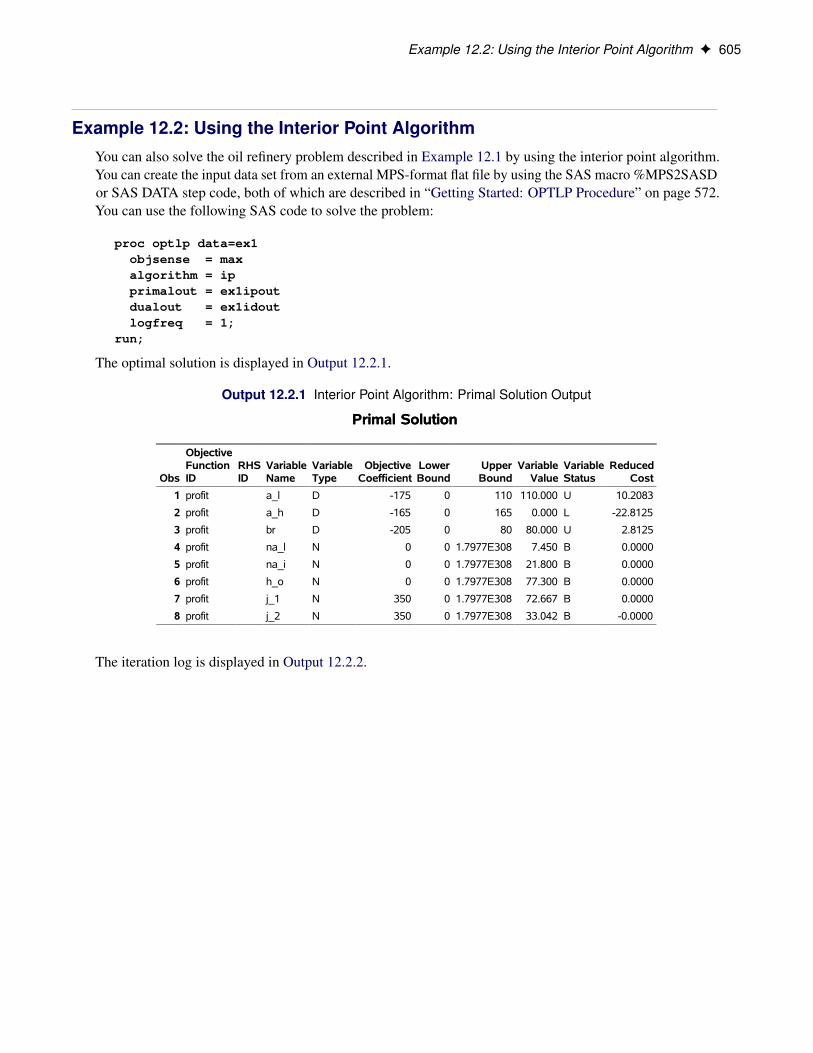
Example 12.2: Using the Interior Point AlgorithmYou can also solve the oil refinery problem described in Example 12.1 by using the interior point algorithm.You can create the input data set from an external MPS-format flat file by using the SAS macro %MPS2SASDor SAS DATA step code, both of which are described in “Getting Started: OPTLP Procedure” on page 572.You can use the following SAS code to solve the problem:
proc optlp data=ex1objsense = maxalgorithm = ipprimalout = ex1ipoutdualout = ex1idoutlogfreq = 1;
run;
The optimal solution is displayed in Output 12.2.1.
Output 12.2.1 Interior Point Algorithm: Primal Solution Output
Primal SolutionPrimal Solution
Obs
ObjectiveFunctionID
RHSID
VariableName
VariableType
ObjectiveCoefficient
LowerBound
UpperBound
VariableValue
VariableStatus
ReducedCost
1 profit a_l D -175 0 110 110.000 U 10.2083
2 profit a_h D -165 0 165 0.000 L -22.8125
3 profit br D -205 0 80 80.000 U 2.8125
4 profit na_l N 0 0 1.7977E308 7.450 B 0.0000
5 profit na_i N 0 0 1.7977E308 21.800 B 0.0000
6 profit h_o N 0 0 1.7977E308 77.300 B 0.0000
7 profit j_1 N 350 0 1.7977E308 72.667 B 0.0000
8 profit j_2 N 350 0 1.7977E308 33.042 B -0.0000
The iteration log is displayed in Output 12.2.2.

606 F Chapter 12: The OPTLP Procedure
Output 12.2.2 Log: Solution Progress
NOTE: The problem EX1 has 8 variables (0 free, 0 fixed).
NOTE: The problem has 6 constraints (3 LE, 3 EQ, 0 GE, 0 range).
NOTE: The problem has 19 constraint coefficients.
WARNING: The objective sense has been changed to maximization.
NOTE: The LP presolver value AUTOMATIC is applied.
NOTE: The LP presolver removed 3 variables and 3 constraints.
NOTE: The LP presolver removed 6 constraint coefficients.
NOTE: The presolved problem has 5 variables, 3 constraints, and 13 constraint
coefficients.
NOTE: The LP solver is called.
NOTE: The Interior Point algorithm is used.
NOTE: The deterministic parallel mode is enabled.
NOTE: The Interior Point algorithm is using up to 4 threads.
Primal Bound Dual
Iter Complement Duality Gap Infeas Infeas Infeas Time
0 8.5854E+01 1.9793E+01 3.0659E+00 1.9225E-02 1.4035E-01 0
1 1.2781E+01 4.0987E+00 3.0659E-02 1.9225E-04 1.8524E-02 0
2 3.1432E+00 5.7077E-01 2.4337E-03 1.5261E-05 5.3069E-03 0
3 4.6086E-01 7.8016E-02 2.3031E-04 1.4441E-06 2.1627E-04 0
4 5.7121E-03 9.4907E-04 3.2096E-06 2.0126E-08 2.5564E-06 0
5 5.7128E-05 9.4891E-06 3.2096E-08 2.0126E-10 2.5564E-08 0
6 0.0000E+00 9.6858E-08 3.9897E-07 6.3643E-13 7.2023E-07 0
NOTE: The Interior Point solve time is 0.00 seconds.
NOTE: The CROSSOVER option is enabled.
NOTE: The crossover basis contains 0 primal and 0 dual superbasic variables.
Objective
Phase Iteration Value Time
P C 1 0.000000E+00 0
P 2 2 1.347916E+03 0
D 2 3 1.347917E+03 0
NOTE: The Crossover time is 0.00 seconds.
NOTE: Optimal.
NOTE: Objective = 1347.9166667.
NOTE: The data set WORK.EX1IPOUT has 8 observations and 10 variables.
NOTE: The data set WORK.EX1IDOUT has 6 observations and 10 variables.
Example 12.3: The Diet ProblemConsider the problem of diet optimization. There are six different foods: bread, milk, cheese, potato, fish,and yogurt. The cost and nutrition values per unit are displayed in Table 12.14.
Table 12.14 Cost and Nutrition Values
Bread Milk Cheese Potato Fish YogurtCost 2.0 3.5 8.0 1.5 11.0 1.0
Protein, g 4.0 8.0 7.0 1.3 8.0 9.2Fat, g 1.0 5.0 9.0 0.1 7.0 1.0
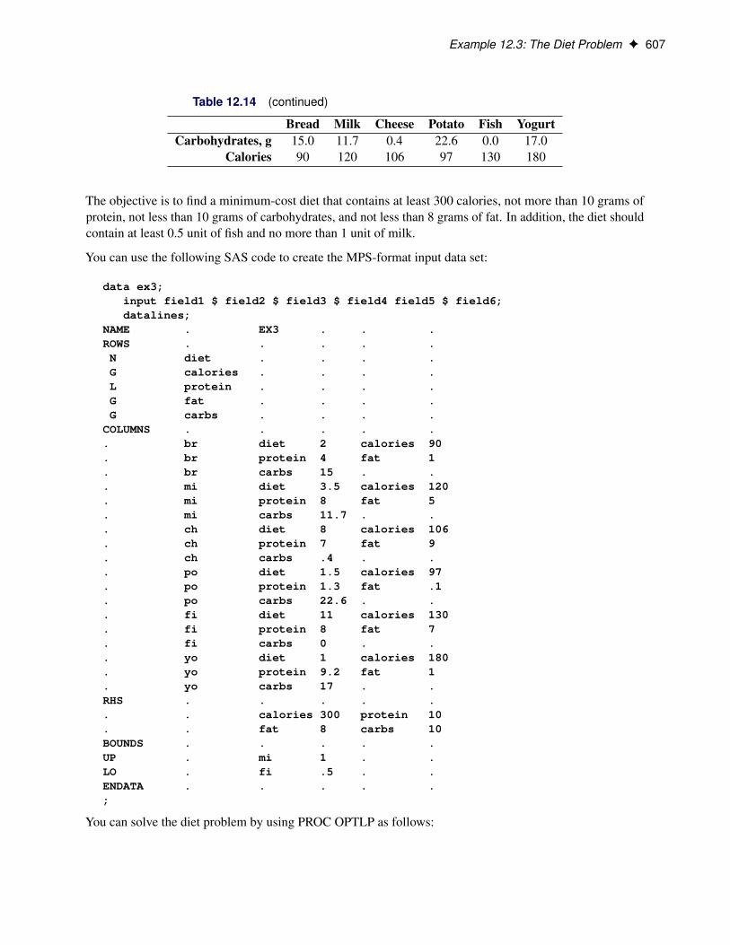
Example 12.3: The Diet Problem F 607
Table 12.14 (continued)
Bread Milk Cheese Potato Fish YogurtCarbohydrates, g 15.0 11.7 0.4 22.6 0.0 17.0
Calories 90 120 106 97 130 180
The objective is to find a minimum-cost diet that contains at least 300 calories, not more than 10 grams ofprotein, not less than 10 grams of carbohydrates, and not less than 8 grams of fat. In addition, the diet shouldcontain at least 0.5 unit of fish and no more than 1 unit of milk.
You can use the following SAS code to create the MPS-format input data set:
data ex3;input field1 $ field2 $ field3 $ field4 field5 $ field6;datalines;
NAME . EX3 . . .ROWS . . . . .N diet . . . .G calories . . . .L protein . . . .G fat . . . .G carbs . . . .
COLUMNS . . . . .. br diet 2 calories 90. br protein 4 fat 1. br carbs 15 . .. mi diet 3.5 calories 120. mi protein 8 fat 5. mi carbs 11.7 . .. ch diet 8 calories 106. ch protein 7 fat 9. ch carbs .4 . .. po diet 1.5 calories 97. po protein 1.3 fat .1. po carbs 22.6 . .. fi diet 11 calories 130. fi protein 8 fat 7. fi carbs 0 . .. yo diet 1 calories 180. yo protein 9.2 fat 1. yo carbs 17 . .RHS . . . . .. . calories 300 protein 10. . fat 8 carbs 10BOUNDS . . . . .UP . mi 1 . .LO . fi .5 . .ENDATA . . . . .;
You can solve the diet problem by using PROC OPTLP as follows:

608 F Chapter 12: The OPTLP Procedure
proc optlp data=ex3presolver = nonealgorithm = psprimalout = ex3poutdualout = ex3doutlogfreq = 1;
run;
The solution summary and the optimal primal solution are displayed in Output 12.3.1.
Output 12.3.1 Diet Problem: Solution Summary and Optimal Primal Solution
Solution SummarySolution Summary
Obs Label1 cValue1 nValue1
1 Solver LP .
2 Algorithm Primal Simplex .
3 Objective Function diet .
4 Solution Status Optimal .
5 Objective Value 12.081337881 12.081338
6 .
7 Primal Infeasibility 8.881784E-16 8.881784E-16
8 Dual Infeasibility 0 0
9 Bound Infeasibility 0 0
10 .
11 Iterations 6 6.000000
12 Presolve Time 0.00 0
13 Solution Time 0.00 0
Primal SolutionPrimal Solution
Obs
ObjectiveFunctionID
RHSID
VariableName
VariableType
ObjectiveCoefficient
LowerBound
UpperBound
VariableValue
VariableStatus
ReducedCost
1 diet br N 2.0 0.0 1.7977E308 0.00000 L 1.19066
2 diet mi D 3.5 0.0 1 0.05360 B 0.00000
3 diet ch N 8.0 0.0 1.7977E308 0.44950 B 0.00000
4 diet po N 1.5 0.0 1.7977E308 1.86517 B 0.00000
5 diet fi O 11.0 0.5 1.7977E308 0.50000 L 5.15641
6 diet yo N 1.0 0.0 1.7977E308 0.00000 L 1.10849
The cost of the optimal diet is 12.08 units.

Example 12.4: Reoptimizing after Modifying the Objective Function F 609
Example 12.4: Reoptimizing after Modifying the Objective FunctionUsing the diet problem described in Example 12.3, this example illustrates how to reoptimize an LP problemafter modifying the objective function.
Assume that the optimal solution of the diet problem is found and the optimal solutions are stored in the datasets ex3pout and ex3dout.
Suppose the cost of cheese increases from 8 to 10 per unit and the cost of fish decreases from 11 to 7 perserving unit. The COLUMNS section in the input data set ex3 is updated (and the data set is saved as ex4) asfollows:
COLUMNS . . . . ....
. ch diet 10 calories 106...
. fi diet 7 calories 130...
RHS . . . . ....
ENDATA;
You can use the following DATA step to create the data set ex4:
data ex4;input field1 $ field2 $ field3 $ field4 field5 $ field6;datalines;
NAME . EX4 . . .ROWS . . . . .N diet . . . .G calories . . . .L protein . . . .G fat . . . .G carbs . . . .
COLUMNS . . . . .. br diet 2 calories 90. br protein 4 fat 1. br carbs 15 . .. mi diet 3.5 calories 120. mi protein 8 fat 5. mi carbs 11.7 . .. ch diet 10 calories 106. ch protein 7 fat 9. ch carbs .4 . .. po diet 1.5 calories 97. po protein 1.3 fat .1. po carbs 22.6 . .. fi diet 7 calories 130. fi protein 8 fat 7

610 F Chapter 12: The OPTLP Procedure
. fi carbs 0 . .
. yo diet 1 calories 180
. yo protein 9.2 fat 1
. yo carbs 17 . .RHS . . . . .. . calories 300 protein 10. . fat 8 carbs 10BOUNDS . . . . .UP . mi 1 . .LO . fi .5 . .ENDATA . . . . .;
You can use the BASIS=WARMSTART option (and the ex3pout and ex3dout data sets from Example 12.3)in the following call to PROC OPTLP to solve the modified problem:
proc optlp data=ex4presolver = nonebasis = warmstartprimalin = ex3poutdualin = ex3doutalgorithm = primalprimalout = ex4poutdualout = ex4doutlogfreq = 1;
run;
The following iteration log indicates that it takes the primal simplex algorithm no extra iterations to solvethe modified problem by using BASIS=WARMSTART, since the optimal solution to the LP problem inExample 12.3 remains optimal after the objective function is changed.
Output 12.4.1 Iteration Log
NOTE: The problem EX4 has 6 variables (0 free, 0 fixed).
NOTE: The problem has 4 constraints (1 LE, 0 EQ, 3 GE, 0 range).
NOTE: The problem has 23 constraint coefficients.
NOTE: The LP presolver value NONE is applied.
NOTE: The LP solver is called.
NOTE: The Primal Simplex algorithm is used.
Objective Entering Leaving
Phase Iteration Value Time Variable Variable
P 2 1 1.098034E+01 0
NOTE: Optimal.
NOTE: Objective = 10.980335514.
NOTE: The Primal Simplex solve time is 0.00 seconds.
NOTE: The data set WORK.EX4POUT has 6 observations and 10 variables.
NOTE: The data set WORK.EX4DOUT has 4 observations and 10 variables.
Note that the primal simplex algorithm is preferred because the primal solution to the original LP is stillfeasible for the modified problem in this case.

Example 12.5: Reoptimizing after Modifying the Right-Hand Side F 611
Example 12.5: Reoptimizing after Modifying the Right-Hand SideYou can also modify the right-hand side of your problem and use the BASIS=WARMSTART option to obtainan optimal solution more quickly. Since the dual solution to the original LP is still feasible for the modifiedproblem in this case, the dual simplex algorithm is preferred. This case is illustrated by using the same dietproblem as in Example 12.3. Assume that you now need a diet that supplies at least 150 calories. The RHSsection in the input data set ex3 is updated (and the data set is saved as ex5) as follows:
...RHS . . . . .. . calories 150 protein 10. . fat 8 carbs 10BOUNDS . . . . .
...
You can use the following DATA step to create the data set ex5:
data ex5;input field1 $ field2 $ field3 $ field4 field5 $ field6;datalines;
NAME . EX5 . . .ROWS . . . . .N diet . . . .G calories . . . .L protein . . . .G fat . . . .G carbs . . . .
COLUMNS . . . . .. br diet 2 calories 90. br protein 4 fat 1. br carbs 15 . .. mi diet 3.5 calories 120. mi protein 8 fat 5. mi carbs 11.7 . .. ch diet 8 calories 106. ch protein 7 fat 9. ch carbs .4 . .. po diet 1.5 calories 97. po protein 1.3 fat .1. po carbs 22.6 . .. fi diet 11 calories 130. fi protein 8 fat 7. fi carbs 0 . .. yo diet 1 calories 180. yo protein 9.2 fat 1. yo carbs 17 . .RHS . . . . .. . calories 150 protein 10. . fat 8 carbs 10BOUNDS . . . . .UP . mi 1 . .

612 F Chapter 12: The OPTLP Procedure
LO . fi .5 . .ENDATA . . . . .;
You can use the BASIS=WARMSTART option in the following call to PROC OPTLP to solve the modifiedproblem:
proc optlp data=ex5presolver = nonebasis = warmstartprimalin = ex3poutdualin = ex3doutalgorithm = dualprimalout = ex5poutdualout = ex5doutlogfreq = 1;
run;
Note that the dual simplex algorithm is preferred because the dual solution to the last solved LP is stillfeasible for the modified problem in this case.
The following iteration log indicates that it takes the dual simplex algorithm just one more phase II iterationto solve the modified problem by using BASIS=WARMSTART.
Output 12.5.1 Iteration Log
NOTE: The problem EX5 has 6 variables (0 free, 0 fixed).
NOTE: The problem has 4 constraints (1 LE, 0 EQ, 3 GE, 0 range).
NOTE: The problem has 23 constraint coefficients.
NOTE: The LP presolver value NONE is applied.
NOTE: The LP solver is called.
NOTE: The Dual Simplex algorithm is used.
Objective Entering Leaving
Phase Iteration Value Time Variable Variable
D 2 1 8.813205E+00 0 calories (S) carbs (S)
D 2 2 9.174413E+00 0
NOTE: Optimal.
NOTE: Objective = 9.1744131985.
NOTE: The Dual Simplex solve time is 0.00 seconds.
NOTE: The data set WORK.EX5POUT has 6 observations and 10 variables.
NOTE: The data set WORK.EX5DOUT has 4 observations and 10 variables.
Compare this with the following call to PROC OPTLP:
proc optlp data=ex5presolver = nonealgorithm = duallogfreq = 1;
run;
This call to PROC OPTLP solves the modified problem “from scratch” (without using the BA-SIS=WARMSTART option) and produces the following iteration log.

Example 12.6: Reoptimizing after Adding a New Constraint F 613
Output 12.5.2 Iteration Log
NOTE: The problem EX5 has 6 variables (0 free, 0 fixed).
NOTE: The problem has 4 constraints (1 LE, 0 EQ, 3 GE, 0 range).
NOTE: The problem has 23 constraint coefficients.
NOTE: The LP presolver value NONE is applied.
NOTE: The LP solver is called.
NOTE: The Dual Simplex algorithm is used.
Objective Entering Leaving
Phase Iteration Value Time Variable Variable
D 2 1 5.500000E+00 0 mi fat (S)
D 2 2 8.650000E+00 0 ch protein (S)
D 2 3 8.925676E+00 0 po carbs (S)
D 2 4 9.174413E+00 0
NOTE: Optimal.
NOTE: Objective = 9.1744131985.
NOTE: The Dual Simplex solve time is 0.00 seconds.
It is clear that using the BASIS=WARMSTART option saves computation time. For larger or more complexexamples, the benefits of using this option are more pronounced.
Example 12.6: Reoptimizing after Adding a New ConstraintAssume that after solving the diet problem in Example 12.3 you need to add a new constraint on sodiumintake of no more than 550 mg/day for adults. The updated nutrition data are given in Table 12.15.
Table 12.15 Updated Cost and Nutrition Values
Bread Milk Cheese Potato Fish YogurtCost 2.0 3.5 8.0 1.5 11.0 1.0
Protein, g 4.0 8.0 7.0 1.3 8.0 9.2Fat, g 1.0 5.0 9.0 0.1 7.0 1.0
Carbohydrates, g 15.0 11.7 0.4 22.6 0.0 17.0Calories, Cal 90 120 106 97 130 180
sodium, mg 148 122 337 186 56 132
The input data set ex3 is updated (and the data set is saved as ex6) as follows:
/* added a new constraint to the diet problem */data ex6;
input field1 $ field2 $ field3 $ field4 field5 $ field6;datalines;
NAME . EX6 . . .ROWS . . . . .N diet . . . .G calories . . . .L protein . . . .G fat . . . .

614 F Chapter 12: The OPTLP Procedure
G carbs . . . .L sodium . . . .
COLUMNS . . . . .. br diet 2 calories 90. br protein 4 fat 1. br carbs 15 sodium 148. mi diet 3.5 calories 120. mi protein 8 fat 5. mi carbs 11.7 sodium 122. ch diet 8 calories 106. ch protein 7 fat 9. ch carbs .4 sodium 337. po diet 1.5 calories 97. po protein 1.3 fat .1. po carbs 22.6 sodium 186. fi diet 11 calories 130. fi protein 8 fat 7. fi carbs 0 sodium 56. yo diet 1 calories 180. yo protein 9.2 fat 1. yo carbs 17 sodium 132RHS . . . . .. . calories 300 protein 10. . fat 8 carbs 10. . sodium 550 . .BOUNDS . . . . .UP . mi 1 . .LO . fi .5 . .ENDATA . . . . .;
For the modified problem you can warm start the primal and dual simplex algorithms to get a solution faster.The dual simplex algorithm is preferred because a dual feasible solution can be readily constructed from theoptimal solution to the diet optimization problem.
Since there is a new constraint in the modified problem, you can use the following SAS code to create a newDUALIN= data set ex6din with this information:
data ex6newcon;_ROW_='sodium '; _STATUS_='A';output;
run;
/* create a new DUALIN= data set to include the new constraint */data ex6din;
set ex3dout ex6newcon;run;

Example 12.6: Reoptimizing after Adding a New Constraint F 615
Note that this step is optional. In this example, you can still use the data set ex3dout as the DUALIN= dataset to solve the modified LP problem by using the BASIS=WARMSTART option. PROC OPTLP validatesthe PRIMALIN= and DUALIN= data sets against the input model. Any new variable (or constraint) in themodel is added to the PRIMALIN= (or DUALIN=) data set, and its status is assigned to be ‘A’. The primaland dual simplex algorithms decide its corresponding status internally. Any variable in the PRIMALIN= andDUALIN= data sets but not in the input model is removed.
The _ROW_ and _STATUS_ columns of the DUALIN= data set ex6din are shown in Output 12.6.1.
Output 12.6.1 DUALIN= Data Set with a Newly Added Constraint
Obs _ROW_ _STATUS_
1 calories U
2 protein L
3 fat U
4 carbs B
5 sodium A
The dual simplex algorithm is called to solve the modified diet optimization problem more quickly with thefollowing SAS code:
proc optlp data=ex6objsense=minpresolver=nonealgorithm=dsprimalout=ex6poutdualout=ex6doutscale=nonelogfreq=1basis=warmstartprimalin=ex3poutdualin=ex6din;
run;
The optimal primal and dual solutions of the modified problem are displayed in Output 12.6.2.
Output 12.6.2 Primal and Dual Solution Output
Primal SolutionPrimal Solution
Obs
ObjectiveFunctionID
RHSID
VariableName
VariableType
ObjectiveCoefficient
LowerBound
UpperBound
VariableValue
VariableStatus
ReducedCost
1 diet br N 2.0 0.0 1.7977E308 0.00000 L 1.19066
2 diet mi D 3.5 0.0 1 0.05360 B 0.00000
3 diet ch N 8.0 0.0 1.7977E308 0.44950 B 0.00000
4 diet po N 1.5 0.0 1.7977E308 1.86517 B 0.00000
5 diet fi O 11.0 0.5 1.7977E308 0.50000 L 5.15641
6 diet yo N 1.0 0.0 1.7977E308 0.00000 L 1.10849
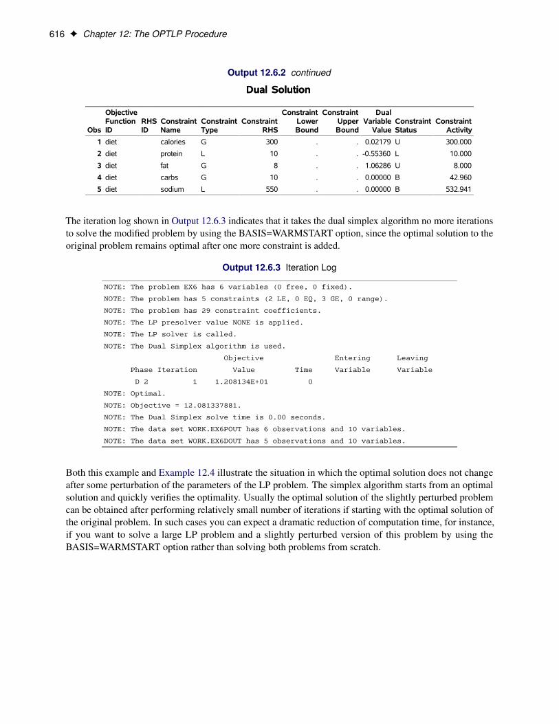
616 F Chapter 12: The OPTLP Procedure
Output 12.6.2 continued
Dual SolutionDual Solution
Obs
ObjectiveFunctionID
RHSID
ConstraintName
ConstraintType
ConstraintRHS
ConstraintLowerBound
ConstraintUpperBound
DualVariableValue
ConstraintStatus
ConstraintActivity
1 diet calories G 300 . . 0.02179 U 300.000
2 diet protein L 10 . . -0.55360 L 10.000
3 diet fat G 8 . . 1.06286 U 8.000
4 diet carbs G 10 . . 0.00000 B 42.960
5 diet sodium L 550 . . 0.00000 B 532.941
The iteration log shown in Output 12.6.3 indicates that it takes the dual simplex algorithm no more iterationsto solve the modified problem by using the BASIS=WARMSTART option, since the optimal solution to theoriginal problem remains optimal after one more constraint is added.
Output 12.6.3 Iteration Log
NOTE: The problem EX6 has 6 variables (0 free, 0 fixed).
NOTE: The problem has 5 constraints (2 LE, 0 EQ, 3 GE, 0 range).
NOTE: The problem has 29 constraint coefficients.
NOTE: The LP presolver value NONE is applied.
NOTE: The LP solver is called.
NOTE: The Dual Simplex algorithm is used.
Objective Entering Leaving
Phase Iteration Value Time Variable Variable
D 2 1 1.208134E+01 0
NOTE: Optimal.
NOTE: Objective = 12.081337881.
NOTE: The Dual Simplex solve time is 0.00 seconds.
NOTE: The data set WORK.EX6POUT has 6 observations and 10 variables.
NOTE: The data set WORK.EX6DOUT has 5 observations and 10 variables.
Both this example and Example 12.4 illustrate the situation in which the optimal solution does not changeafter some perturbation of the parameters of the LP problem. The simplex algorithm starts from an optimalsolution and quickly verifies the optimality. Usually the optimal solution of the slightly perturbed problemcan be obtained after performing relatively small number of iterations if starting with the optimal solution ofthe original problem. In such cases you can expect a dramatic reduction of computation time, for instance,if you want to solve a large LP problem and a slightly perturbed version of this problem by using theBASIS=WARMSTART option rather than solving both problems from scratch.

Example 12.7: Finding an Irreducible Infeasible Set F 617
Example 12.7: Finding an Irreducible Infeasible SetThis example demonstrates the use of the IIS= option to locate an irreducible infeasible set. Suppose youwant to solve a linear program that has the following simple formulation:
min x1 C x2 C x3 .cost/subject to x1 C x2 � 10 .con1/
x1 C x3 � 4 .con2/4 � x2 C x3 � 5 .con3/
x1; x2 � 0
0 � x3 � 3
The corresponding MPS-format SAS data set is as follows:
/* infeasible */data exiis;
input field1 $ field2 $ field3 $ field4 field5 $ field6;datalines;NAME . . . . .ROWS . . . . .N cost . . . .G con1 . . . .L con2 . . . .G con3 . . . .
COLUMNS . . . . .. x1 cost 1 con1 1. x1 con2 1 . .. x2 cost 1 con1 1. x2 con3 1 . .. x3 cost 1 con2 1. x3 con3 1 . .RHS . . . . .. rhs con1 10 con2 4. rhs con3 4 . .RANGES . . . . .. r1 con3 1 . .BOUNDS . . . . .UP b1 x3 3 . .ENDATA . . . . .;
It is easy to verify that the following three constraints (or rows) and one variable (or column) bound form anIIS for this problem.
x1 C x2 � 10 .con1/x1 C x3 � 4 .con2/
x2 C x3 � 5 .con3/x3 � 0
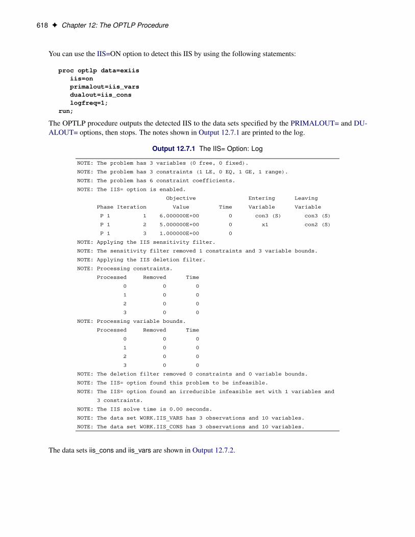
618 F Chapter 12: The OPTLP Procedure
You can use the IIS=ON option to detect this IIS by using the following statements:
proc optlp data=exiisiis=onprimalout=iis_varsdualout=iis_conslogfreq=1;
run;
The OPTLP procedure outputs the detected IIS to the data sets specified by the PRIMALOUT= and DU-ALOUT= options, then stops. The notes shown in Output 12.7.1 are printed to the log.
Output 12.7.1 The IIS= Option: Log
NOTE: The problem has 3 variables (0 free, 0 fixed).
NOTE: The problem has 3 constraints (1 LE, 0 EQ, 1 GE, 1 range).
NOTE: The problem has 6 constraint coefficients.
NOTE: The IIS= option is enabled.
Objective Entering Leaving
Phase Iteration Value Time Variable Variable
P 1 1 6.000000E+00 0 con3 (S) con3 (S)
P 1 2 5.000000E+00 0 x1 con2 (S)
P 1 3 1.000000E+00 0
NOTE: Applying the IIS sensitivity filter.
NOTE: The sensitivity filter removed 1 constraints and 3 variable bounds.
NOTE: Applying the IIS deletion filter.
NOTE: Processing constraints.
Processed Removed Time
0 0 0
1 0 0
2 0 0
3 0 0
NOTE: Processing variable bounds.
Processed Removed Time
0 0 0
1 0 0
2 0 0
3 0 0
NOTE: The deletion filter removed 0 constraints and 0 variable bounds.
NOTE: The IIS= option found this problem to be infeasible.
NOTE: The IIS= option found an irreducible infeasible set with 1 variables and
3 constraints.
NOTE: The IIS solve time is 0.00 seconds.
NOTE: The data set WORK.IIS_VARS has 3 observations and 10 variables.
NOTE: The data set WORK.IIS_CONS has 3 observations and 10 variables.
The data sets iis_cons and iis_vars are shown in Output 12.7.2.

Example 12.7: Finding an Irreducible Infeasible Set F 619
Output 12.7.2 Identify Rows and Columns in the IIS
Constraints in the IISConstraints in the IIS
Obs
ObjectiveFunctionID
RHSID
ConstraintName
ConstraintType
ConstraintRHS
ConstraintLowerBound
ConstraintUpperBound
DualVariableValue
ConstraintStatus
ConstraintActivity
1 cost rhs con1 G 10 . . . I_L .
2 cost rhs con2 L 4 . . . I_U .
3 cost rhs con3 R . 4 5 . I_U .
Variables in the IISVariables in the IIS
Obs
ObjectiveFunctionID
RHSID
VariableName
VariableType
ObjectiveCoefficient
LowerBound
UpperBound
VariableValue
VariableStatus
ReducedCost
1 cost rhs x1 N 1 0 1.7977E308 . .
2 cost rhs x2 N 1 0 1.7977E308 . .
3 cost rhs x3 D 1 0 3 . I_L .
The constraint x2 C x3 � 5, which is an element of the IIS, is created by the RANGES section. Theoriginal constraint is con3, a “�” constraint with an RHS value of 4. If you choose to remove the constraintx2 C x3 � 5, you can accomplish this by removing con3 from the RANGES section in the MPS-formatSAS data set exiis. Since con3 is the only observation in the section, the identifier observation can also beremoved. The modified LP problem is specified in the following SAS statements:
/* dropping con3, feasible */data exiisf;
input field1 $ field2 $ field3 $ field4 field5 $ field6;datalines;NAME . . . . .ROWS . . . . .N cost . . . .G con1 . . . .L con2 . . . .G con3 . . . .
COLUMNS . . . . .. x1 cost 1 con1 1. x1 con2 1 . .. x2 cost 1 con1 1. x2 con3 1 . .. x3 cost 1 con2 1. x3 con3 1 . .RHS . . . . .. rhs con1 10 con2 4. rhs con3 4 . .BOUNDS . . . . .UP b1 x3 3 . .ENDATA . . . . .;
Since one element of the IIS has been removed, the modified LP problem should no longer contain theinfeasible set. Due to the size of this problem, there should be no additional irreducible infeasible sets. Youcan confirm this by submitting the following SAS statements:

620 F Chapter 12: The OPTLP Procedure
proc optlp data=exiisfiis=on;
run;
The notes shown in Output 12.7.3 are printed to the log.
Output 12.7.3 The IIS= Option: Log
NOTE: The problem has 3 variables (0 free, 0 fixed).
NOTE: The problem has 3 constraints (1 LE, 0 EQ, 2 GE, 0 range).
NOTE: The problem has 6 constraint coefficients.
NOTE: The IIS= option is enabled.
Objective
Phase Iteration Value Time
P 1 1 1.400000E+01 0
P 1 3 0.000000E+00 0
NOTE: The IIS= option found this problem to be feasible.
NOTE: The IIS solve time is 0.00 seconds.
NOTE: The data set WORK.EXSS has 8 observations and 3 variables.
The solution summary is displayed in Output 12.7.4.
Output 12.7.4 Infeasibility Removed
Solution SummarySolution Summary
Obs Label1 cValue1 nValue1
1 Solver LP .
2 Algorithm IIS .
3 Objective Function cost .
4 Solution Status Feasible .
5 .
6 Iterations 3 3.000000
7 Presolve Time 0.00 0
8 Solution Time 0.00 0
Example 12.8: Using the Network Simplex AlgorithmThis example demonstrates how to use the network simplex algorithm to find the minimum-cost flow in adirected graph. Consider the directed graph in Figure 12.5, which appears in Ahuja, Magnanti, and Orlin(1993).

Example 12.8: Using the Network Simplex Algorithm F 621
Figure 12.5 Minimum-Cost Network Flow Problem: Data
2
20
6
0
1b = 10 3
0
5
0
8 −10
4
−5
7
−15
(2, 15)
(1, 10)
(0, 10)
(c = 6, u = 10)
(1, 5)
(4, 10)
(5, 10)
(2, 20)
(7, 15)
(8, 10)
(9, 15)
You can use the following SAS statements to create the input data set ex8:
data ex8;input field1 $8. field2 $13. @25 field3 $13. field4 @53 field5 $13. field6;datalines;
NAME . . . . .ROWS . . . . .N obj . . . .E balance['1'] . . . .E balance['2'] . . . .E balance['3'] . . . .E balance['4'] . . . .E balance['5'] . . . .E balance['6'] . . . .E balance['7'] . . . .E balance['8'] . . . .COLUMNS . . . . .. x['1','4'] obj 2 balance['1'] 1. x['1','4'] balance['4'] -1 . .. x['2','1'] obj 1 balance['1'] -1. x['2','1'] balance['2'] 1 . .. x['2','3'] balance['2'] 1 balance['3'] -1. x['2','6'] obj 6 balance['2'] 1. x['2','6'] balance['6'] -1 . .. x['3','4'] obj 1 balance['3'] 1. x['3','4'] balance['4'] -1 . .. x['3','5'] obj 4 balance['3'] 1. x['3','5'] balance['5'] -1 . .. x['4','7'] obj 5 balance['4'] 1. x['4','7'] balance['7'] -1 . .. x['5','6'] obj 2 balance['5'] 1. x['5','6'] balance['6'] -1 . .. x['5','7'] obj 7 balance['5'] 1. x['5','7'] balance['7'] -1 . .. x['6','8'] obj 8 balance['6'] 1. x['6','8'] balance['8'] -1 . .

622 F Chapter 12: The OPTLP Procedure
. x['7','8'] obj 9 balance['7'] 1
. x['7','8'] balance['8'] -1 . .RHS . . . . .. .RHS. balance['1'] 10 . .. .RHS. balance['2'] 20 . .. .RHS. balance['4'] -5 . .. .RHS. balance['7'] -15 . .. .RHS. balance['8'] -10 . .BOUNDS . . . . .UP .BOUNDS. x['1','4'] 15 . .UP .BOUNDS. x['2','1'] 10 . .UP .BOUNDS. x['2','3'] 10 . .UP .BOUNDS. x['2','6'] 10 . .UP .BOUNDS. x['3','4'] 5 . .UP .BOUNDS. x['3','5'] 10 . .UP .BOUNDS. x['4','7'] 10 . .UP .BOUNDS. x['5','6'] 20 . .UP .BOUNDS. x['5','7'] 15 . .UP .BOUNDS. x['6','8'] 10 . .UP .BOUNDS. x['7','8'] 15 . .ENDATA . . . . .;
You can use the following call to PROC OPTLP to find the minimum-cost flow:
proc optlppresolver = noneprintlevel = 2logfreq = 1data = ex8primalout = ex8outalgorithm = ns;
run;
The optimal solution is displayed in Output 12.8.1.
Output 12.8.1 Network Simplex Algorithm: Primal Solution Output
Primal SolutionPrimal Solution
Obs
ObjectiveFunctionID
RHSID
VariableName
VariableType
ObjectiveCoefficient
LowerBound
UpperBound
VariableValue
VariableStatus
ReducedCost
1 obj .RHS. x['1','4'] D 2 0 15 10 B 0
2 obj .RHS. x['2','1'] D 1 0 10 0 L 2
3 obj .RHS. x['2','3'] D 0 0 10 10 B 0
4 obj .RHS. x['2','6'] D 6 0 10 10 B 0
5 obj .RHS. x['3','4'] D 1 0 5 5 B 0
6 obj .RHS. x['3','5'] D 4 0 10 5 B 0
7 obj .RHS. x['4','7'] D 5 0 10 10 U -5
8 obj .RHS. x['5','6'] D 2 0 20 0 L 0
9 obj .RHS. x['5','7'] D 7 0 15 5 B 0
10 obj .RHS. x['6','8'] D 8 0 10 10 B 0
11 obj .RHS. x['7','8'] D 9 0 15 0 L 6
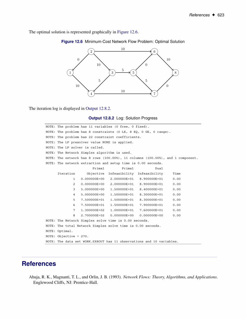
References F 623
The optimal solution is represented graphically in Figure 12.6.
Figure 12.6 Minimum-Cost Network Flow Problem: Optimal Solution
2 6
1 3 5 8
4 7
10
0
10
10
5
5
10
0
5
10
0
The iteration log is displayed in Output 12.8.2.
Output 12.8.2 Log: Solution Progress
NOTE: The problem has 11 variables (0 free, 0 fixed).
NOTE: The problem has 8 constraints (0 LE, 8 EQ, 0 GE, 0 range).
NOTE: The problem has 22 constraint coefficients.
NOTE: The LP presolver value NONE is applied.
NOTE: The LP solver is called.
NOTE: The Network Simplex algorithm is used.
NOTE: The network has 8 rows (100.00%), 11 columns (100.00%), and 1 component.
NOTE: The network extraction and setup time is 0.00 seconds.
Primal Primal Dual
Iteration Objective Infeasibility Infeasibility Time
1 0.000000E+00 2.000000E+01 8.900000E+01 0.00
2 0.000000E+00 2.000000E+01 8.900000E+01 0.00
3 5.000000E+00 1.500000E+01 8.400000E+01 0.00
4 5.000000E+00 1.500000E+01 8.300000E+01 0.00
5 7.500000E+01 1.500000E+01 8.300000E+01 0.00
6 7.500000E+01 1.500000E+01 7.900000E+01 0.00
7 1.300000E+02 1.000000E+01 7.600000E+01 0.00
8 2.700000E+02 0.000000E+00 0.000000E+00 0.00
NOTE: The Network Simplex solve time is 0.00 seconds.
NOTE: The total Network Simplex solve time is 0.00 seconds.
NOTE: Optimal.
NOTE: Objective = 270.
NOTE: The data set WORK.EX8OUT has 11 observations and 10 variables.
References
Ahuja, R. K., Magnanti, T. L., and Orlin, J. B. (1993). Network Flows: Theory, Algorithms, and Applications.Englewood Cliffs, NJ: Prentice-Hall.

624 F Chapter 12: The OPTLP Procedure
Andersen, E. D., and Andersen, K. D. (1995). “Presolving in Linear Programming.” MathematicalProgramming 71:221–245.
Chinneck, J. W. (2008). Feasibility and Infeasibility in Optimization: Algorithms and Computational Methods.Vol. 118 of International Series in Operations Research and Management Science. New York: Springer.
Dantzig, G. B. (1963). Linear Programming and Extensions. Princeton, NJ: Princeton University Press.
Forrest, J. J., and Goldfarb, D. (1992). “Steepest-Edge Simplex Algorithms for Linear Programming.”Mathematical Programming 5:1–28.
Gondzio, J. (1997). “Presolve Analysis of Linear Programs Prior to Applying an Interior Point Method.”INFORMS Journal on Computing 9:73–91.
Harris, P. M. J. (1973). “Pivot Selection Methods in the Devex LP Code.” Mathematical Programming57:341–374.
Maros, I. (2003). Computational Techniques of the Simplex Method. Boston: Kluwer Academic.

Subject Index
_ACTIVITY_ variableDUALOUT= data set, 587
basis, 580
concurrent LP, 593
data, 576decomposition algorithm
OPTLP procedure, 582distributed mode
OPTLP procedure, 582DUALIN= data set
OPTLP procedure, 583, 584variables, 583, 584
dualization, 578DUALOUT= data set
OPTLP procedure, 585–587variables, 585–587
feasibility tolerance, 579
IIS optionOPTLP procedure, 597
irreducible infeasible setOPTLP procedure, 597
iteration logcrossover algorithm, 592interior point algorithm, 592network simplex algorithm, 591OPTLP procedure, 590–592primal and dual simplex algorithms, 590
_LBOUND_ variablePRIMALOUT= data set, 584
linear programming, see also OPTLP procedure_L_RHS_ variable
DUALOUT= data set, 586
OROPTLP_OROPTLP_, 599
multithreadingOPTLP procedure, 582
_VAR_ variablePRIMALOUT= data set, 584
_OBJ_ID_ variableDUALOUT= data set, 585PRIMALOUT= data set, 584
ODS table names
OPTLP procedure, 594OPTLP examples
diet optimization problem, 606finding an irreducible infeasible set, 617oil refinery problem, 601reoptimizing after adding a new constraint, 613reoptimizing after modifying the objective
function, 609reoptimizing after modifying the right-hand side,
611using the interior point algorithm, 605using the network simplex algorithm, 620
OPTLP procedurealgorithm, 577basis, 580concurrent LP, 593crossover, 582data, 576decomposition algorithm, 582definitions of DUALIN= data set variables, 583,
584definitions of DUALOUT= data set variables,
585, 586definitions of DUALOUT=data set variables, 586,
587definitions of PRIMALIN data set variables, 583definitions of PRIMALIN= data set variables, 583definitions of PRIMALOUT= data set variables,
584, 585distributed mode, 582dual infeasibility, 582DUALIN= data set, 583, 584duality gap, 582dualization, 578DUALOUT= data set, 585–587feasibility tolerance, 579functional summary, 575IIS option, 597interior point algorithm, 589introductory example, 572iteration log, 590–592multithreading, 582network simplex algorithm, 588ODS table names, 594_OROPTLP_ macro variable, 599preprocessing, 578presolver, 578pricing, 581

primal infeasibility, 582PRIMALIN= data set, 583PRIMALOUT= data set, 584, 585problem statistics, 596queue size, 581random seed, 581scaling, 581single-machine mode, 582
presolver, 578pricing, 581PRIMALIN= data set
OPTLP procedure, 583variables, 583
PRIMALOUT= data setOPTLP procedure, 584, 585variables, 584, 585
queue size, 581
random seed, 581_R_COST_ variable
PRIMALOUT= data set, 585_RHS_ variable
DUALOUT= data set, 586_RHS_ID_ variable
DUALOUT= data set, 586PRIMALOUT= data set, 584
_ROW_ variableDUALIN= data set, 583DUALOUT= data set, 586
scaling, 581single-machine mode
OPTLP procedure, 582_STATUS_ variable
DUALIN= data set, 584DUALOUT= data set, 586PRIMALIN= data set, 583PRIMALOUT= data set, 585
_TYPE_ variableDUALOUT= data set, 586PRIMALOUT= data set, 584
_UBOUND_ variablePRIMALOUT= data set, 585
_U_RHS_ variableDUALOUT= data set, 586
_VALUE_ variableDUALOUT= data set, 586PRIMALOUT= data set, 585
_VAR_ variablePRIMALIN= data set, 583PRIMALOUT= data set, 584
Syntax Index
ALGORITHM2= optionPROC OPTLP statement, 578
ALGORITHM= optionPROC OPTLP statement, 577
BASIS= optionPROC OPTLP statement, 580
CROSSOVER= optionPROC OPTLP statement, 582
DATA= optionPROC OPTLP statement, 576
DECOMP_MASTER statementOPTLP procedure, 582
DECOMP statementOPTLP procedure, 582
DECOMP_SUBPROB statementOPTLP procedure, 582
DUALIN= optionPROC OPTLP statement, 576
DUALIZE= optionPROC OPTLP statement, 578
DUALOUT= optionPROC OPTLP statement, 576
FEASTOL= optionPROC OPTLP statement, 579
IIS= optionPROC OPTLP statement, 577
LOGFREQ= optionPROC OPTLP statement, 579
LOGLEVEL= optionPROC OPTLP statement, 579
MAXITER= optionPROC OPTLP statement, 579
MAXTIME= optionPROC OPTLP statement, 580
OBJSENSE= optionPROC OPTLP statement, 576
OPTLP procedure, 575DECOMP_MASTER statement, 582DECOMP statement, 582DECOMP_SUBPROB statement, 582PERFORMANCE statement, 582
OPTTOL= option
PROC OPTLP statement, 580
PERFORMANCE statementOPTLP procedure, 582
PRESOLVER= optionPROC OPTLP statement, 578
PRICETYPE= optionPROC OPTLP statement, 581
PRIMALIN= optionPROC OPTLP statement, 577
PRIMALOUT= optionPROC OPTLP statement, 577
PRINTFREQ= optionPROC OPTLP statement, 579
PRINTLEVEL2= optionPROC OPTLP statement, 579
PRINTLEVEL= optionPROC OPTLP statement, 580
PROC OPTLP statementALGORITHM2= option, 578ALGORITHM= option, 577BASIS= option, 580CROSSOVER= option, 582DATA= option, 576DUALIN= option, 576DUALIZE= option, 578DUALOUT= option, 576FEASTOL= option, 579IIS= option, 577LOGFREQ= option, 579LOGLEVEL= option, 579MAXITER= option, 579MAXTIME= option, 580OBJSENSE= option, 576OPTTOL= option, 580PRESOLVER= option, 578PRICETYPE= option, 581PRIMALIN= option, 577PRIMALOUT= option, 577PRINTFREQ= option, 579PRINTLEVEL2= option, 579PRINTLEVEL= option, 580QUEUESIZE= option, 581SAVE_ONLY_IF_OPTIMAL option, 577SCALE= option, 581SEED= option, 581SOL= option, 577SOLVER2= option, 578

SOLVER= option, 577STOP_DG= option, 582STOP_DI= option, 582STOP_PI= option, 582TIMETYPE= option, 580
QUEUESIZE= optionPROC OPTLP statement, 581
SAVE_ONLY_IF_OPTIMAL optionPROC OPTLP statement, 577
SCALE= optionPROC OPTLP statement, 581
SEED= optionPROC OPTLP statement, 581
SOL= optionPROC OPTLP statement, 577
SOLVER2= optionPROC OPTLP statement, 578
SOLVER= optionPROC OPTLP statement, 577
STOP_DG= optionPROC OPTLP statement, 582
STOP_DI= optionPROC OPTLP statement, 582
STOP_PI= optionPROC OPTLP statement, 582
TIMETYPE= optionPROC OPTLP statement, 580