iOD

D.&E.CORNICKSAA.N .MIC HEL0• MARCH 1972

I

[SU-ERI-AMES- 72072

THE NUMERICAL OPTIMIZATIONOF DISTRIBUTED PARAMETER SYSTEMSBY GRADIENT METHODS

CONTRACT NO. N000'14.68.A.0162 L EJULJOFFICE OF NAVAL RESEARCHDEPARTMENT OF THE NAVYWASHINGTON. D. C. 20360

DISTRflý blVý A-,dumt a ,ilboi m isNonfnriI", Approved fac p.b.ic r' -o'-e

~iki* 3u~aa.UamiuL sptoduc~d by?ajetJ2SNATIONAL TECHNICAL

INFORMATION SERVICESpringfield, Vs. 22151

1 I-,km

ENGINEERINGRESEARCHENGINEERINGRESEARCHENGINEERINGRESEARCHENGINEERINGRESEARCHENGINEERINGRESEARCH

TECHNICAL REPORT

THE NUMERICAL OPTIMIZATION OF

DISTRIBUTED PARAMETER SYSTEMSBY GRADIENT METHODS

D. E. CornickA. N. MichelMarch 1972

Duplication of this report, in whole or in part.

may be made for any purpose of the, Uniled Statesgovernmmnt

Prevlmred and, r Th,,mis ConrtruitNo. N000 14 68A 01(12for ()'ficf. ,f Navult R,'searth

I)"pIrtnment ofsth; Navy"Wahinrtoni,.D.. 20360 ENGINEERING RESEARCH INSTITUTE

ISU-ERI-AMES-72072 IOWA STATE UNIVERSITY AMES

Unclassified

DOCUMENT CONTROL DATA- R & D

I lii.rjINA TI NG AC TIVI tY ',piri tt *iItt t) ,41. I C( RP 1 %1 CU I' I 'I C'L A r-..III C. A 1 101,

Engineering Research Institute UnclassifiedIowa State University yh,. GrOUP

N/A1 $4 POt 14 1 T 1T1

THE NUMERICAL OPTIMIZATION OF DISTRIBUTED PARAMETER SYSTEMS BY GRADIENT METHODS

4 L)ESCRIP T I VE NOTES (TylPr Ai ?1,:p(,ft anti. 1-t 1- lll,' 4,hi.t )

Technical Reportn AU THONiSi (Ftirs name, liddle inlital, Ila, nflllml)

Douglas E. CornickAnthony N. Michel

6. RqEPORT )At'E 7. TOTAL NO OF PAGES lb. NO OF REFS

March 1972 147 1,67IN. CON TRACT OR GRANT NO. 90. ORIGINATOW'S REPORT TIUMBERIS)

Themis Contract N0014-68-A-0162 ERI-72072h. PROJECT NO.

9?. OTHER REPORT NOiSt (Any ather rumbars that Imay be ait,ilga•,rlthis report)

d. None

10 OISTRIBUTION STATEMENT

Distribution of this document is unlimited.

It SUPPLIML:NTARY NOTES 12 SPONSORING MILITARY ACTIVITY

Department of the NavyOffice of Naval ResearchWashington, DC. 20360

13 A•rTRACT

Th. numerical optimization of distributed parameter systems is considered. Inparticular the adaptation of the Davidon method, the conjugate gradient method, andthe "best step" steepest descent method to distributed parameters is presented. Theclass of problems with quadratic cost functionals and linear dynamics is investigated.Penalty functions are used to render constrained problems amenable to these gradienttechniques.

Also considered is an analysis of the effects of discretization of continuousdistributed parameter optimal control problems. Estimates of discretization errorbounds are established and a measure of the suboptimality of the numerical solution ispresented.

Numerical results for both the constrained and the unconstrained optimal controlof the one-dimensional wave equation are given. Both the distributed and theboundary control of the wave equation are treated. The standard numerical comparisonsbetween the Davidon method, the conjugate gradient method, and the steepest descentmethod are reported. It is evident from these comparisons that both the Davidonmethod and the conjugate gradient method offer a substantial improvement over thesteepest descent method.

Some of the numerical considerations, such as, selection of appropriate finitedifference methods, multiple quadrature formulas, interpolating formulas, storage re-quirements, computer run-times, etc. are also considered.

P0RM DPA(G I).DD NOV ,1473 UnclassifiedS/N 01 01-07-6811 Securitv Classification A-3140A

A-310

UnclassifiedSecurity Classifi'ation

14 LINK A LINK 8 LINK

ROLE WY ROLE WT POLL WT

Optimal Control

Numerical Optimization

Distributed Parameter Systems

Steepest Descent

Conjugate Gradients

Davidon Method

Error Analysis

Discretization Errors

Roundoff Errors

Distributed Optimal Controls

Boundary Optimal Controls

State Constraints

Penalty Function

Wave Equation

Heat Equation

DD ,NOO ..141 3 (BACK) Unclassified/N 0101.-807-6821 Security Clagssfication A- ?1I 409

THE NUMERICAL OPTIMIZATION OF DISTRIBUTED PARAMETER

SYSTEMS BY GRADIENT METHODS

ABSTRACT

The numerical optimization of distributed parameter systems is

considered. In particular the adaptation of the Davidon method, the

conjugate gradient method, and the "best step" steepest descent method

to distributed parameters is presented. The class of problems with

quadratic cost functionals and linear dynamics is investigated. Penalty

functions are used to render constrained problems amenable to these

gradient techniques.

Also considered is an analysis of the effects of discretization of

continuous distributed parameter optimal control problems. Estimates

of discretization error bounds are established and a measure of the

suboptimality of the numerical solution is presented.

Numerical results for both the constrained and the unconstrained

optimal control of the one-dimensional wave equation are given. Both

the distributed and the boundary control of the wave equation are treated.

The standard numerical comparisons between the Davidon method, the

conjugate gradient method, and the steepest descent method are reported.

It is evident from these comparisons that both the Davidon method and

the conjugate gradient method offer a substantial improvement over the

steepest descent method.

Some of the numerical considerations, such as, selection of ap-

propriate finite difference methods, multiple quadrature formulas,

interpolating formulas, storage requirements, computer run-times, etc.

are also considered.

TABLE OF CONTENTS

Page

. ABSTRACT i

LIST OF FIGURES iv

LIST OF TABLES v

CHAPTER I. INTRODUCTION 1

Results Concerning the Problem Formulation 3

Results Concerning the Problem Solution 5

Engineering Applications 7

Dissertation Objectives 8

Class of Problems Considered 10

Dissertation Outline 11

CHAPTER II. THE OPTIMAL CONTROL OF DISTRIBUTEDPARAMETER SYSTEMS 14

The Optimal Control Problem 14

The Distributed Parameter Optimal ControlProblem 16

Conditions for Optimality 19

Methods of Solution 24

CHAPTER III. INTRODUCTION TO GRADIENT METHODS 26

Gradient Method Algorithm 28

General Results for Gradient Methods 40

CHAPTER IV. AN APPROXIMATION THEORY FOR GRADIENTMETHODS 42

The Effects of the Discrete Approximations onthe Gradient Vector 46

The Effects of Gradient Error on GradientMethods 55

Error Estimates 68

Determination of the Parameters in theError Estimates 77

iii

Page

Geometric Interpretation of the Error Bounds 80

CHAPTER V. NUMERICAL RESULTS 84

CHAPTER VI. CONCLUDING REMARKS 111

LITERATURE CITED 118

ACKNOWLEDGMENTS 124

APPENDIX A. MATHEMATICAL PRELIMINARIES 125

Selected Results from Functional Analysis 125

Pertinent Results from Partial DifferentialEquations 133

Pertinent Results from Approximation Theoryand Numerical Analysis 136

APPENDIX B. THE NON-LINEAR DISTRIBUTED PARAMETER

OPTIMAL CONTROL PROBLEM 141

Problem Formulation 141

Derivation of the Necessary Conditions 142

Optimality Conditions 146

DISTRIBUTTON LIST

iv

LIST OF FIGURES

Page

Figure 3.1. The gradient method algorithm. 30

Figure 4.1. The discretization process. 51

Figure 4.2. Cubic interpolation. 62

Figure 4.3. The regula falsi iterator. 66

Figure 4.4. Geometrical interpretation of the optinal controlerror. 81

Figure 4.5. Constant cost contours. 82

Figure 4.6. Minimization on a subspace. 83

Figure 5.1. The vibrating string. 85

Figure 5.2. The solution to the unconstrained minimum energydistributed control of the vibrating string(Rf = 1.0 and Tf = 1.0). 95

Figure 5.3. The vibrating string. 96

Figure 5.4. The constrained minimum energy distributed controlof the vibrating string, a = 100. 98

n

Figure 5.5. Boundary control of the vibrating string. 103

Figure 5.6. The solution of the minimum energy boundary controlof the vibrating string. 108

Figure 5.7. The solution of the minimum energy boundary controlof the vibrating string. 109

Figure A-I. The node N of the net M. 139

v

LIST OF TABLES

Page

Table 5.1. Summary of equations for example 5.1. 89

Table 5.2. Results for example 5.1. 91

Table 5.3. Penalty constants for the solution of the constrainedvibrating string problem. 97

Table 5.4. The solution of the constrained vibrating stringproblem. 99

Table 5.5. The solution of example 5.2 with a trigometricinitial condition (i.e., x 0 (r) = sin nr). 101

Table 5.6. The solution of example 5.2 with a non-trigonometricinitial condition (i.e., x0(r) = r(l - r)). 102

Table 5.7. Summary of equations for example 5,3. 104

Table 5.8. Results for example 5.3 with u (t) 0. 106

Table 5.9. Results of example 5.3 with u (t) = - lOet cos 2rrt. 107

0

'I

[1

CHAPTER I. INTRODUCTION

The optimal control of distributed parameter systems is

concerned with the minimization (maximization) of functionals

constrained by either nonhomogeneous partial differential

equations or by multiple integral equations. The study of

the optimal control of distributed parameter systems is

generally considered to have been initiated in 1960 by

Butkovskii and Lerner (1). The term "distributed parameter

system" was coined by Butkovskii and was intended to refer to

dynamical systems which are modeled by either partial dif-

ferential equations or by multiple integral equations. In

fact, it is these distributed constraints which distinguishes

this field from the classical multi-variable calculus of

variations, which was considered by Lagrange as early as 1806.

The optimal control of distributed parameter systems

has received considerable attention in recent years. Since

Butkovskii and Lerner's original paper, well over two hundred

publications have appeared in the literature concerned with

this subject. At the present time two full length books

(2, 3) have been published on this topic and more are in

preparation. In addition many of the recent texts on optimi-

zation include chapters introducing this subject (4, 5). Also,

a number of doctoral dissertations have reported results on

various aspects of this field (6, 7, 8 and 9).

The rapid growth of literature concerning this topic has

I'

2

motivated a number of recent survey papers on this subject,

which include extensive bibliographies. The first survey of

the subject was generated by Wang (10) in 1964 and still

provides a good introduction to the subject. Subsequently,

Wang published an extensive bibliography covering both the

stability and the optimal control of distributed Parameter

systems (11). In 1968 Butkovskii, Egorov and Lurie (12)

published an excellent survey of the Soviet efforts in this

field. In 1969, Robinson compiled what is probably the most

complete bibliogranhy of this subject to date (13). Robinson

includes in his bibliography a brief discussion of manv of

the various facets of this topic. Due to the existence of

these recent survey papers, only a brief introduction to

distributed parameter systems will be given; and a complete

bibliography will be omitted.

At the present time there is no universally accepted

method for classifying the works published on this subject.

A number of possibilities are discussed in (13). In the sub-

sequent discussion, the publications will be divided into two

groups: (1) those papers which are primarily concerned with

the mathematical structure of the problem formulation; and

(2) those results which are primarily concerned with the

problem solution.

3

Results Concerning the ProblemFormulation

The majority of the papers on the optimal control of dis-

tributed parameter systems deal primarily with the extensions

of the theoretical results obtained for lumped parameter

systems to distributed parameter systems. In fact about one-

half of all the reports, which have appeared in the literature,

are concerned with the problem formulation giving particular

attention to the derivation of the necessary conditions for

optimality. Three basic approaches have been utilized in

the derivation of these necessary conditions: (1) variational

calculus; (2) dynamic programming; and (3) functional analysis.

In addition, there is the method of moments which can be used

if che functional is constrained by a system of linear integral

equations (14). In his early works, Butkovskii (15, 16) con-

siders systems described by integral equations and employs

variational methods to derive the necessary conditions for

optimality. These necessary conditions are given in the form

of integral equations. A number of Butkovskii's subsequent

works are concerned with the development of methods for solving

these integral equations. Egorov (17) and Lurie (18) follow

the work of Butkovskii; however, they consider systems described

by partial differential equations. Both of these approaches

have their advantages and their disadvantages. Since the

integral representation of the dynamical system yields bounded

4

operators, this approach is useful in theoretical develop-

ments. However, the differential representation of dynamical

systems, which unfortunately introduces unbounded operators,

is useful because many physical problems are easily formulated

in terms of partial dilferential equations. In principle at

least, Green's functions can be employed to convert linear

partial differential equations into linear integral equations.

However, in practice this is not always possible, certainly

not in general for the non-linear case.

Wang was one of the first to use dynamic proqramminq to

derive the necessary conditions for distributed parameter

systems with distributed control. Brogan (6) extends Wang's

results to include boundary control. The functional analysis

methods are generally applied to abstract optimal control

problems in either a Banach space or in a Hilbert space. With

this degree of generality, the results obtained in these

papers certainly can be applied to distributed parameter

systems and to lumped parameter control problems as well.

Papers by Balakrishnan (19, 20) are of particular interest to

the present investigation; since in these papers, Balakrishnan

considers the extension of the classica' steepest descent

method to the general Hilbert space setting. Russell (21)

applies functional analysis methods to problems in which the

controls are finite-dimensional. Axelband (22) utilizes the

Fre6het derivative to obtain the necessary conditions for a

LM

5

quadratic functional. He then proceeds to develop methods

for solving the resulting linear operator equation. A

number of authors, for example (23, 24 and 25) utilize

certain properties of special classes of problems to develop

methods for obtainiing the optimal control.

Results Concerning the ProblemSolution

In the optimization of distributed parameter systems,

one's first impulse is to transform the problem into some

other form which can be solved by existing techniques. This

approach leads ultimately to some type of approximation. At

the present, the following approximations have been tried:

(1) eigenvector expansion; (2) spacial discretization; and

(3) space-time discretization. Of course, the eigenvector

(eigenfunction is the term usually used in this case) ex-

pansion techniques are classical methods of approximating

partial differential equations. Unfortunately, this method

only works for linear or linearized problems with rather

restrictive boundary conditions. When this method does

apply, the distributed parameter problem is reduced to a

lumped parameter problem. An approximation is introduced when

the eigenvector expansion is truncated to a finite number of

terms in order to facilitate a practical solution. Lukes and

Russell (26) prove that the solution obtained from the

truncated eigenvector expansion converges to the exact solu-

I

6

tion of the distributed parameter problem as the number of

terms in the expdnsion increases. Space discretization also

reduces the problem to an approximate lumped parameter

problem. However, a very large number of ordinary differential

equations result from this method; and conventional lumped

parameter methods have not proven to be very effective in this

case. Axelband (22) uses space-time discretization to reduce

the problem to a parameter optimization problem. However,

once again the number of independent variables becomes ex-

tremely large; and difficulties are encountered in obtaining

the solution with standard techniques. Axelband also proves

that in the limit this method converges to the true solution.

However, in doing so, he neglects to consider the numerical!

approximations and their effects on the convergence of the

method. Recently, a number of authors (27, 28, 29 and 30)

have alluded to the fact that some of the direct computational

methods developed for the solution of lumped parameter opti-

mization problems, especially gradient methods, might also be

beneficially extended to distributed parameter systems. At

the present time computational experience with the steepest

descent method, as related to the optimization of distributed

parameter systems, has been reported in (28, 29 and 30).

These methods offer the advantages of beina very simple and

of applying to a broad class of problems.t

7

Engineering Applications

In recent years considerations of the control of complex

processespsuch as nuclear reactors and chemical production

systems, have motivated interest in the optimal control of

distributed parameter systems. However, these are not the

only possible applications for this theory. For example, it

is clear that an optimal control theory for distributed

parameter systems can be applied to the process industries

(chemical, petroleum, steel, cement, glass, etc.), the power

industry, and the aerospace industry. The following list is

not complete; nevertheless, it does indicate the variety of

problem areas to which the optimal control theory of

distributed parameter systems could be applied:

1. Control of heat and mass transfer processes (e.g.,heating, cooling, melting, drying, etc.).

2. Control of fluid dynamic processes (e.g., pumpingof petroleum, hydroelectric power generation,liquid rocket engine design, acoustic phenomena,etc.).

3. Control of chemical and kinetic reactions (e.g.,petroleum refining, production of steel and glass,combustion processes, chemical industries, etc.).

4. Control of elastic and viscoelastic vibrations (e.g.,heavy equipment industry, aerospace industry,geographic applications, location of petroleumdeposits, etc.).

5. Control of nuclear and atomic processes (e.g.,nuclear power industry, nuclear space propulsionsystems, nuclear energy propagation, etc.).

6. Control of radioactive processes (e.g., radiationshielding, optical and electro-magnetic communica-tions, etc.).

7. Control of hydrodynamical and magnetohydrodynamicprocesses.

8. Control of spacecraft attitude (e.g., heat dissi-pation, structural effects, etc.).

9. Control of melting, freezing, and crystal growth.

10. Control of environmental processes (e.g., airpollution, water pollution, flood control, trafficcontrol, forest fire control, etc.).

After examining the above list, it becomes immediately apparent

that there is no lack of motivation (from the point of view

of applications) for the theory of optimal control of dis-

tributed parameter systems.

Dissertation Objectives

As mentioned before, many of the existing results to

date are concerned with the mathematical structure of the

problem and the derivation of the necessary conditions for

optimality. Unfortunately, very little has been said con-

cerning how to solve these necessary conditions to obtain the

optimal control. From the engineerinq point of view, the

problem solution is at least as important as the problem

formulation. Therefore, it seems desirable that a large

amount of future research efforts should be devoted to the

development of methods for solving the problems already

formulated.

One of the original objectives of the present research

was to demonstrate numerically that the second generation

9I

gradient methods, such as the conjugate gradient method and

the Davidon method, could be efficiently adapted to solve

practical distributed parameter problems. These methods were

selected because of their simplicity, their generality, and

their success in solving lumped parameter optimal control

problems. However, preliminary storage requirement calcu-

lations indicate that the solution of realistic distributed

parameter optimization problems are beyond the present

storage capabilities of the Model 360-65 system. In addition,

early inmerical results indicate that the approximations in-

volved in discretizing the continuous problem are causing

substantial errors in the approximate solution. It was

realized that in order to effectively solve distributed optimal

control problems by gradient methods, it is essential to

determine the effects of these approximations on the numerical

solution. The new objectives formulated are: (1) to develop

a general optimization theory for a particular class of

distributed parameter problems; (2) to isolate those approxi-

mations which cause the largest errors in the numerical solu-

tion for this class of problems; (3) to determine the effects

of these errors on the class of gradient methods; (4) to

develop estimates for the errors between the exact and the

approximate solution; (5) to evaluate the effectiveness of the

conjugate gradient method and the Davidon method in comparison

with the standard steepest descent method on this class of

10

problems; and (6) to generate numerical results which sub-

stantiate the theory developed in objectives (1) through (5).

Class of Problems Considered

The non-linear distributed parameter optimal control

problem is easily formulated; and if the existence of a rela-

tive minimum is assumed, the derivation of the necessary con-

ditions for optimality is straight forward. However, the

solution of a non-linear distributed parameter optimal control

problem is usually very difficult. Existence and uniqueness

considerations for both the minimizing element and the

distributed dynamical system dictate that extreme care be

exercised in the selection of the class of problems to be

considered.

Fortunately, gradient methods do not require the a

priori assumption of the existence of a relative minimum.

However, they do require the existence and uniqueness of the

solutions of the dynamical system. Thus, the selection of the

distributed dynamical system to be optimized is an important

consideration in distributed parameter problems.

The second generation gradient methods are basically un-

constrained, quadratic functional, optimization methods. Thus,

it seems natural to investigate their performance on quadratic

distributed parameter problems, especially, since quadratic

problems play such a significant role in the present state of

1i

the art of distributed parameter systems. The penalty function

approach can be used to alter the constrained distributed

parameter optimal control problem into an unconstrained, quad-

ratic functional, optimization problem; if: (1) the penalty

functional is quadratic; (2) the original cost index is

quadratic; and (3) the distributed parameter dynamical system

is linear. In the following, only problems with the above

properties will be considered; and will be referred to as

quadratic programming problems.

Dissertation Outline

The distributed parameter optimal control problem is

formulated in Chapter II. Phe concept of a functional deri-

vative is utilized to derive the expression for the gradient

of the cost index. Brief remarks are made concerning methods

which use the gradient to obtain the optimal control.

Gradient methods are introduced in Chapter III.

Specifically, an introduction of the three most popular

gradient methods is presented. The concepts of the inner and

outer loop iterations are discussed, and popular inner loop

iterators are introduced.

The development of an approximation theory for the

numerical solution of distributed parameter systems by

gradient methods is presented in Chapter IV. The definitions

of the Optimal Control Error and the Cost Functional Error

12

are introduced. It is shown that the approximations involved

in the discretization of the continuous problem cause gradient

errors. The effects of gradient error on gradient methods is

analyzed. Error estimates for the approximate numerical

solution are developed. A geometrical interpretation of these

error estimates is presented.

Chapter V presents numerical results for both the con-

strained and the unconstrained optimal control of the one-

dimensional wave equation. Both :.•tributed %control and

boundary control are considered. Penalty functions are used

to render the constrained problem amenable to the gradient

methods. Standard numerical comparisons between the conjugate

gradient method, the Davidon method, and the steepest descent

method are given. Some of the numerical considerations, such

as selection of appropriate finite-difference methods,

multiple quadrature formulas, storage requirements, computer

run times, etc., are discussed

Concluding remarks and recommendations for additional re-

search are given in Chapter VI.

Appendix A introduces mathematical concepts which are

pertinent to this dissertation. The coverage of these topics

is extremely brief; consequently, it is not intended to be an

introduction to any of the areas discussed, but rather as a

point of reference for the development presented in the main

body of this work.

rI13

In Appendix B the derivation of the necessary conditions

for a general non-linear distributed parameter optimal control

problem is presented. Ordinary differential equations on the

spatial boundary are considered. The standard calculus of

variations is employed in the derivation of the necessary con-

ditions for optimality.

14

CHAPTER II. THE OPTIMAL CONTROL OF DISTRIBUTED

PARAMETER SYSTEMS

The Optimal Control Problem

The optimal control problem may be stated as follows:

minimize

J(u;x], (2.1) Isubject to

J[u;x] > 0, xEX and ucU; (2.2)

where X is called the state space, U the set of admissible

controls, and J[u;x] is a real valued functional defined on

the product space U x X. The non-linear operator 4 is de-

fined on U x X, and 0 is the null vector of this product space.

The functional J[.;.] is generally referred to as the cost

index, and the conditions of Equation 2.2 are called the

constraints. As a consequence of the constraints, the state

trajectory x(t) is dependent upon the control u. Thus any

particular optimal control problem depends on the nature of

the functions J and 1P, and on the sets X and U. Consider

the following special cases: 1. Parameter Optimization:

let X and U be real Euclidean vector spaces, let 4 be a vector

valued function, and let J be a scalar valued function;

2. Lumped Parameter Optimization: let X and U be properly

selected function spaces, let 0 be decomposed into two

operators T and S, where T represents an algebraic equality

15

and/or inequality constraint, and where S denotes a differen-

tial and/or integral operator with respect to one variable,

and let J be a real valued functional; 3. Distributed

Parameter Optimization: let X and U be properly selected

function spaces, let i be composed of algebraic, differential

and/or integral operators with respect to more than one

variable, and let J be a real valued functional. The solu-

tion of problems formulated in case 3 (above) is the topic

of this dissertation.

The difficulties encountered in solving for the optimal

control of a distributed parameter system are generally

related to the complexity of the constraints, Equation 2.2.

For distributed parameter systems very few general results

are available concerning the existence and uniqueness of the

solution to the constraint equation. Consequently, little

can be said regarding the solution of the general distributed

parameter problem. However, there exist certain classes of

problems, of practical significance, for which results can be

obtained. For one such important class one lets: (1)

J[u;x] be a quadratic functional in u and x; and (2) it[u;x] be

a linear equality constraint. It is this particular class of

distributed parameter problems which will be considered

in what follows.

I ro

16

The Distributed Parameter OptimalControl Problem

Cost index

Let J[u;x] be a real valued quadratic functional defined

on the real separable Hilbert space U x X, generated by the

self-adjoint operators M and N, and by the inner product

<.,.>, and let J[u;x] be specified by

J0u;x] = co + <clu> + 12<UMu> + <c 2 ,x> + (2.3)

or

[u1J;X] C c0 + < [0 b

+ 2 u [ I [ dIN1M ub

+ <c 2x> + 1<x,NX>, (2.4)21 1

where XC L 2[ xT ], UC:L 2[ XT ], Rm, T •R 1 c 0 cR C l, U

c2cX, and where the vector c2 and the operator M are parti-

tioned i and [Md Mb],respectively. At any time teT

the distributed state of the system is denoted by

I!

17

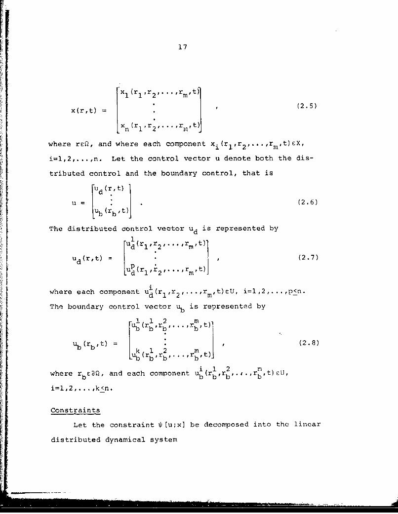
x(r,t) (2.5)

x n (rl,r ,. r rin, t

where rEQ, and where each component x (rl,r 2 ,...,rmit) £X,

i=i,2,...,n. Let the control vector u denote both the dis-

tributed control and the boundary control, that is

1ud (r,t)1U (2.6)

Ub (rb ,t)

The distributed control vector ud is represented by

u lr .00r t)1S1 2 1.

ud(r,t) = • (2.7)dr uP(rlr, .,rm,t)]

where each component ud(rl,r 2 ,...,rm,t)kU, i=l,2,...,p<n.

The boundary control vector ub is represented by

1 r2 rMt).

ub b,...? ,b~t

ub(rb 2 (2.8)b br'b•

i 1 2 m

where rhbE9, and each component ub(r, rb" .. ,rb t)9U,

i=l,2,... ,k<n.

Constraints

Let the constraint [ tu;xl be decomposed into the linear

distributed dynamical system

18

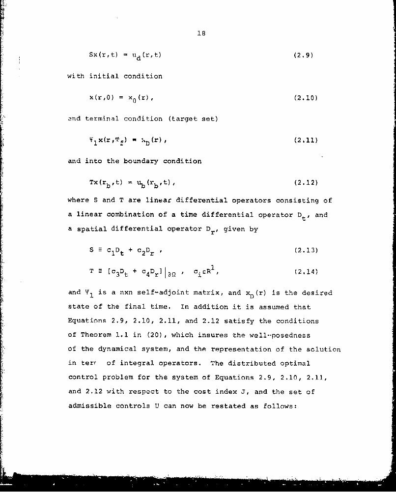
Sx(r,t) = ud(r,t) (2.9)

with initial condition

x(r,0) - x0 (r), (2.10)

and terminal condition (target set)

I- D(r) , (2.11)

and into the boundary condition

Tx(rb,t) = u(rbt), (2.12)

where S and T are linear differential operators consisting of

a linear combination of a time differential operator Dt, and

a spatial differential operator Dr, given by

S E clDt + c2Dr (2.13)

T [c 3 Dt + c 4 Dr] W , cicR1 , (2.14)

and Y is a nxn self-adjoint matrix, and xD (r) is the desired

state of the final time. In addition it is assumed that

Equations 2.9, 2.10, 2.11, and 2.12 satisfy the conditions

of Theorem 1.1 in (20), which insures the well--posedness

of the dynamical system, and the representation of the solution

in terr of integral operators. The distributed optimal

control problem for the system of Equations 2.9, 2.10, 2.11,

and 2.12 with respoct to the cost index J, and the set of

admissible controls U can now be restated as follows:

II

19

determine the control u*eU such that

J [u*;x(u*)] = min{Jf u;x(u)]} . (2.15)u£U

Conditions for Optimality

Existence of an optimum

For the class of problems considered the existence and

the uniqueness of the minimizing element u* can be easily

proven (31). This, of course, is certainly not the case

for the general distributed parameter optimal control problem,

since existence and uniqueness results for even the dynamical

system do not (in general) exist. The existence and unique-

ness of the solution was one of the primary reasons for the

selection of this particular class of problems, as the

subject of the present investigation.

Derivation of the necessary conditions for optimality

The numerical methods which are used in this dissertation

are directly applicable to only the unconstrained problem.

Thus, it is convenient to transform this constrained

problem into some equivalent unconstrained problem.

Assume that the distributed dynamical system defined by

Equations 2.9 through 2.12 satisfy the conditions of Theorem

1.1 (20); this insures that the dynami!al system has a unique

solution for all uEU. However, only the controls in a subset

20

U CU drive the system from the initial state to the target

set. Therefore, the specification of a target set causes the

dynamical system to generate a constraint in the control

space. Hence, strictly speaking only the controls uU T are

admissible, since if uE[UT] the u does not satisfy all of

"the constraints.

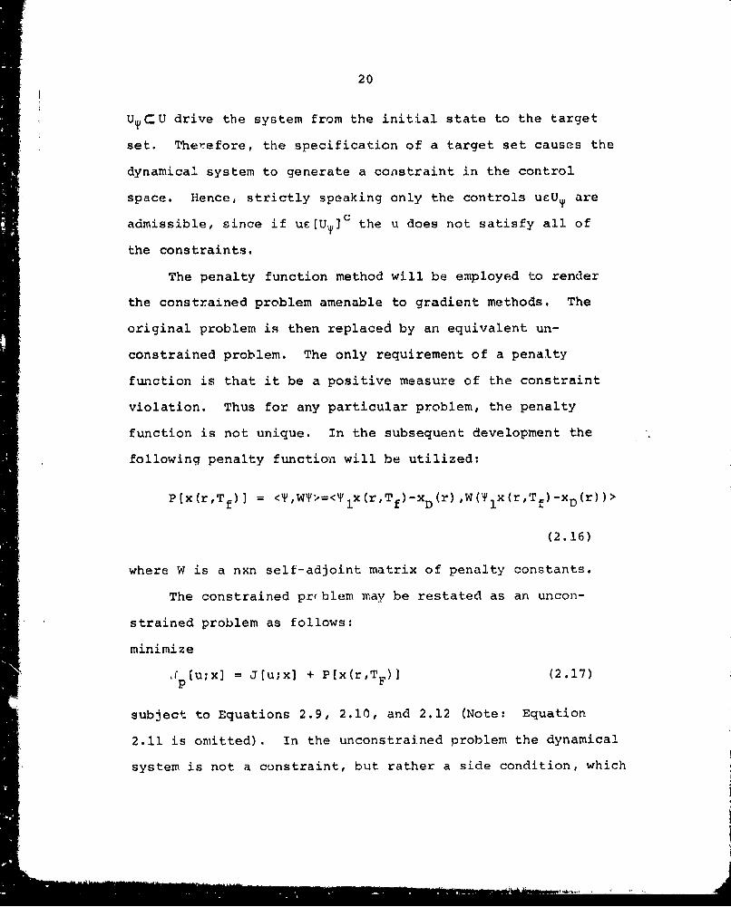
The penalty function method will be employed to render

the constrained problem amenable to gradient methods. The

original problem is then replaced by an equivalent un-

constrained problem. The only requirement of a penalty

function is that it be a positive measure of the constraint

violation. Thus for any particular problem, the penalty

function is not unique. In the subsequent development the

following penalty function will be utilized:

P[x(rTf)] = <T,W'>=<Ylx(r,Tf)-xD(r),W(Tlx(r,Tf)-xD(r))>

(2.16)

where W is a nxn self-adjoint matrix of penalty constants.

The constrained pr blem may be restated as an uncon-

strained problem as follows:

minimize

Jp[(u;x] = J[u;x] + P[x(r,TF)] (2.17)

subject to Equations 2.9, 2.10, and 2.12 (Note: Equation

2.11 is omitted). In the unconstrained problem the dynamical

system is not a constraint, but rather a side condition, which

21

must be solved only to evaluate the penalized cost index J pBy representing the solution of the state system in terms

of appropriate Green's functions it is possible to remove the

explicit dependence of the cost index on the state trajectory.

Thus, let the solution of the dynamical system exist, be

unique, and have the representation

x(r,t) = 4,(t)x 0 (r) + S-(t)ud(r,t) + T-Jt)ub(rb,t), (2.18)

where N(t)x 0 (r) denotes thi contribution to the solution at

time t due to the initial conditions, S-td(rt) denotes

the contribution to the solution at time t due to thE Os--l

tributed control, and T (t)ub(rb,t) denotes the contribuLion

to the solution at time t due to the boundary control. The

state of the system at the time Tf is then denoted by-l -l

x(rTf) = D(Tf)x 0 (r) + S (Tf )ud(r,t) + T (Tf)ub(rb't).

(2.19)

The state trajectory is eliminated from the penalized

cost index by substituting Equations 2.18 and 2.19 into

Equation 2.17, i.e.,

-1 -1J p[uxl = J [u;O(t)x 0 +S (t)Ud+T (t)ub]

-1 -1+ P[O(Tf)X 0 +S (Tf)ud + T (Tf)ub]. (2.20)

Simplification of Equation 2.20 yields the standard quadratic

form

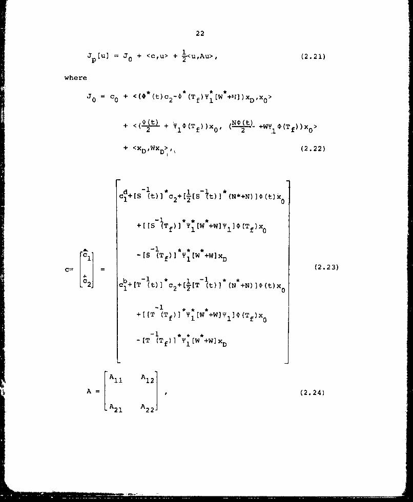
22

JU] = + <c,u> + I<u,Au>, (2.21)

where

* + <(t c*

+ <(+* + (T (P(Tf) x No[W t) +WY D (Tf)) x>

+ <XDWXD>,1 (2.22)

c -1S W 10 [~-i1*.N+),(~1 22

+[II -T)l *" T[w * +w] ly O(T )x°

[ -IS (Tf)] i(W +WIxD

C= (2.23)

[21 c1+[T (t)] c2 +[-[T (t) * (N +N)]•(t)x0

+[[T (Tf)] •i [W +W]Y l](TTf)x0

- [T (Tf) 1l (W +W]XD

A l A[24

A =(2.24)

A 21 A2 22-

23

with

Al1-Md+IS (t)] NS (t)+2[S Tf)] •IWTiS (Tf), (2.25)

-1 * -d -If], T f

A1 2i[S (t)] NT (t)+2[S (Tf)S YIW•T (Tf), (2.26

S[-it ]* -1 -1

A 21 [T t)] NS (t)+2[T (Tff)] I WY SITf), (2.27)A21--f

-1 , -1 -1 , • -1A22=Mb+[T (t)] NT (t)+2[T (T.f Y1WY1T (Tf) (2.28)

The necessary condition for u* to be the element of U

which minimizes Jp is that the gradient (utilizinq the Fre~hetPU

derivative) of J with respect to the control u vanish at u*.P

Thus

f uA i = g(u*) = c + i[A+A*lu* = 0. (2.29)

If A is a self-adjoint operator, then Equation 2.29 yields

g(u*) = c + Au* = 0 . (2.30)

From Equations 2.25 through 2.28 it follows that for A to be

self-adjoint, Md, Mb, N, Ti' and W must he self-adjoint. If

A is self-adjoint then the Hessian of Jp given by

(22•u- •A, (2.31)

i I i i

24

is positive definite. Consequently Equations 2.30 and 2.3].

are necessary and sufficient conditions for u* to exist and

be the unique optimal control for the penalized cost index Jp'

Methods of Solution

This dissertation is not primarily concerned with

formulating necessary conditions for optimality, but rather

in developing practical methods for solving distributed

parameter optimal control problems. Thus, a brief introduction

of the basic optimization methods is warranted. In the opti-

mization literature two basic classifications for the methods

of solution have evolved. These categories are generally

referred to as the direct and the indirect methods.

Indirect methods

Indirect methods are those methods which determine the

optimal control by indirectly solving (in most cases

iteratively) the operator equation

g(u) = 0 . (2.32)

In general Equation 2.32 is used to eliminate the control from

the state and costate systems. Once the control is elimi-

nated, the state and the costate systems form the classical

two point boundary value problem (TPBV). The optimal control

can be determined once this TPBV problem is solved. Most

N ir.

25

indirect methods are characterized by an iterative modification

of either the boundary conditions and/or the partial dif-

ferential equations.

Direct methods

Direct methods are those methods which determine the

optimal control by directly operating on the cost index J.

Based on information concerning J and possibly the gradient

of J the direct methods result in an iterative procedure

which, hopefully, converges to the optimal control. These

methods require an initial guess to start the iteration, and

then correct this initial guess in a certain predetermined

manner. The various direct methods differ principally in

the means used to determine the control correction. The

gradient methods which are certainly the most popular of this

class of direct methods will be discussed in more detail in

the following chapter.

26

CHAPTER III. INTRODUCTION TO

GRADIENT METHODS

Gradient methods are direct optimization methods which

utilize derivative information during the iteration. The

most well-known of the classical gradient methods are the

steepest descent method and the Newton-Raphson method. The

steepest descent method is a first order method (i.e., it

uses first derivative information) which is characterized by

simple logic, stability with respect to the initial guess, and

slow convergence near the solution. In contrast to the

steepest descent method is the Newton-Raphson method, a

second order method which exhibits rapid convergence near

the solution, but poor stability with respect to the initial

guess. In recent years a class of second generation gradient

methods have been developed which combine the simplicity and

stability of the first order methods with the convergence

properties of the second order methods. The most popular of

this class of gradient methods are the conjugate gradient

method and the Davidon method. Although, the motivation for

each of these two methods is different, their performance is

strikingly similar. In fact, these two methods (theoretical-

ly) produce identical iterations on quadratic problems (32).

At the present time only the standard steepest descent

method has been adapted to the optimization of distributed

parameter systems. In this dissertation the numerical

I\•

27

adaptation of the conjugate gradient method and the Davidon

method to distributed parameter systems is presented,

In general, gradient methods are employed to design

computer algorithms which are used to obtain approximate

solutions to optimization problems. These algorithms usually

consist of two iterative processes, which are interrelated.

The terms "outer loop iterator" and "inner luop iterator"

are introduced to denote these two iterative processes. The

reasons for this designation will become apparent when the

algorithm is introduced.

Before presenting the general gradient algorithm some

nomenclature and definitions have to be intrdocued. Let the

control, the gradient, the direction of search, and the

control correction parameter at the nth iteration be denoted

by un, gn' Sn and yn' respectively; where Un cU for all

n>O, gncG for all n>O, Sn ES for all n>O, and for all

n>O, and where U, G, and S are real separable Hilbert spaces.

In the cases to be considered spaces G, S, and U are iden-

tical.

Definition 3.1: The outer loop iterator, specified by the

particular gradient method employed, implicitly determines

the direction of search sn and explicitly performs the control

iteration; and is given by

28

Un+1 OL(UYn,Yn Unil,...,Un-m), (3.1)

n-mwhere OL: R x fl U-U, and m denotes the number of back

i=0

points used in the iteration.

Remarks: 1. The semicolon in Equation 3.1 separates the point

at which new data are used from the point at

which old data are reused.

2. The iteration formula defined by Equation 3.1

is referred to as a one point iterator with

memory (33).

Definition 3.2: The inner loop iterator determines the

control correction parameter yn' and is given by

Yni+l i(Ys], , g(u +YnS (3.2)n L(nIJ(Un+yn n n n n(32where

11IL: R xR xUxU-R

Gradient Method Algorithm

The interrelationship between the inner loop and the

outer loop iterators is best illustrated in the gradient

method algorithm. This algorithm is as follows:

Outer loop iteration

1. For n=O, guess an initial control function u0 .

I!29

2. Calculate the gradient of the cost functional

g(un) = gn by:

a. integrating the state system from t 0 to Tf;

b. integrating the costate system backwards

from Tf to to.

3. Calculate the direction of search sn.

4. Inner loop iteration: calculate the control

correction parameter yn.

5. Calculate the control correction.

6. Test the convergence criteria; if these tests are

not satisfied, increase n and repeat computations

beginning with step 2.

The logic flow chart for the above algorithm is presented

in Figure 3.1.

The various gradient methods differ principally in the

means used to determine the direction of search s (step 3),n

and the control correction parameter yn (step 4). The

conjugate gradient method and the Davidon method are outer

loop iterators with memory, whereas the steepest descent

method is an outer loop method without memory, i.e.,

steepest descent always searches in the negative gradient

direction. Thus, the conjugate gradient method and the Davidon

method are able to utilize the results of previous iterates

to improve the direction of search; and hence converge more

rapidly than the methods without memory.

30

GUESS u

CALCULATE

IF YES

-• '~~OR ALL y >0

CALCULATEFINDUn+= TG(uHAT

n NJ

I ,,I = G(n sn

r 3. -h g en; - - a- l

Figure 3.1. The gradient method algorithm

V

:i 31

Outer loop iterators

The approximation theory developed in the next chapter

applies to gradient methods in general. However, numerical

results will be presented for only the following three

gradient methods: the steepest descent method, the con-

jugate gradient method, and the Davidon method. A brief

introduction to each of these methods is presented below.

The steepest descent method The steepest descent

method is perhaps the oldest of the direct search methods.

This method was originall" developed for minimizing a function

defined on a real Euclidean vector !rppce. An account of this

method was given as early as 1847 by Cauchy. Later, it

was named the method of gradients by Hadamard. In 1945 the

steepest descent method was extended to the case where the

function is defined on a Hilbert space (34). More recently

Bryson et al. (35, 36) and Kelley (37) have used the steepest

descent method to solve lumped parameter optimal control

problems. Several authors (9, 28, 29 and 30) have applied

the steepest descent method to the distributed parameter

optimal control problem.

The basic philosophy of the steepest descent method is

very simple. The maximum rate of decrease of J in a neighbor-

hood of an admissible control u is in the direction definedn

by -g This direction defines the half-ray unl Un-Ygn, Y>O.

Thus to obtain the maximum decrease in the cost index, the

it

32

best local direction of search is in the negative gradient

direction; hence, the method is named steepest descent.

Consequently the outer loop iterator is given by

Un+1 un - (3.3)

where the control correction parameter yn is determined by

the inner loop iterator.

It is important to note that in the general case the

direction of search s defines the direction of maximumn

decrease in J only for yn arbitrarily small. In practice

the selection of small control correction parameters leads

to excessive iterations. In fact to insure that {Un )}U*,

Yn must be bounded away from zero. If yN=0 for some N>O,

then uN becomes a fixed point of the outer loop iterator;.

but gN is not necessarily the null vector, and hence uN is

not necessarily the minimizing element u*. The slow

convergence of the steepest descent method near the solution

can be attributed to the fact that as the iteration converges

the gradient tends to the null vector. Hence, the control

correction YnIIgnl becomes excessively small, unless proper

piecautions are taken in the selection of yn. This brief

discussion indicates the importance of the inner loop

iterator.

The simplicity and the stability of the steepest descent

method enables it to be adapted to many difficult, practical

/:3

'f

33

problems. These characteristics are important to practicing

engineers, and they often outweigh the slow convergence

* properties ot the steepest descent method.

The conjugate gradient method The conjugate gradient

method was originally developed as a method for solving a set

of linear algebraic equations; the solution of the set of

equations being related to the minimum (maximum) of a certain

properly selected cost index (38). In 1954 Hayes (39)

extended the original conjugate gradient method to linear

operator equations in a Hilbert space. Since then (40)

and (41) have also considered the adaptation of this method

to the solution of linear operator equations. Fletcher and

Reeves (42) then modified the conjugate gradient method and

used it to develop a parameter optimization algorithm.

Lasdon et al. (43), and Sinnott and Luenberger (44) extended

the conjugate gradient method to lumped parameter optimal

control problems.

The conjugate gradient method is a gradient method with

memory. The motivation for this method is given by the follow-

ing considerations. Let the set of admissible controls U be a

real, separable Hilbert space, i.e., U contains a countable dense

subset. The separability insures the existence of at least

one linearly independent set of basis vectors {s n}, S nU,

such that the finite-dimensional subspaces Bn spanned by

( 's0sl...,Sn-1) form an expanding sequence of subspaces,

34

whose union is the closure of the control space. If for each

n>0, the inner loop iterator minimizes J over the translation

of the one-dimensional subspace defined by Un+l=Un+YS1, then

J[u n+l]=J[Un+Ynsn)_J[un+Ysn] for all y>O, (3.4)

and

J[Un+ 2 ]=Jtun+l4'yn+lSn+l ]<J[un+l+Ysn+l] for all y>0.

(3.5)

Thus, two one-dimensional minimizations are sequentially per-

formed over a translation of the subspaces spanned by sn and

Sn+l' respectively. The following important question now

arises. How can the direction of search sn+1 be selected

such that the result of this sequence of two one-dimensional

minimizations give the same solution as would a two-dimensional

minimization over the translation of the two-dimensional sub-

space spanned by (sn ,Sn+l That is, how should sn+l be deter-

mined such that

J[un+2 ]<J[un+asn+asn+l] for all a>0 and 8>0. (3.6)

The conjugate gradient method generates such an outer loop

iterator. This means that the solution obtained by performing

a sequence of one-dimensional minimizations over a properly

selected set of translated subspaces yields the minimum of

the functional over the translated subspace spanned by this

set. This method is referred to as the "method of expanding

subspaces".

At the present time there exist two versions of the

conjugate gradient method; the original version is developed

in (38), and the modified version is developed in (45).

Willoughby (46), presents an excellent discussion and com-

parison of these two versions; and demonstrates numerically

that on quadratic functionals these two methods do not

produce identical iterations as the theory predicts. Never-

theless, the modified version requires substantially less com-

putation; hence, it will be utilized in what follows.

In the modified conjugate gradient method the direction

of search is determined as follows:

Sn = -n + Bnn 1 '(3.7)

n ~n n-l

where B <gn' gn>

B n n (3.8)n <g n-l' gn-i>

if n=O, then B0=0.

The outer loop iterator for the conjugate gradient method is

given by

un+l = un + Yn n (3.9)

The second term on the right hand side of Equation 3.7 is

the nmemory element. This term deflects the direction of

search from the negative gradient direction. The modified

conjugate gradient method is particularly simple to program,

I,-_J

36

requires little additional computation and storage in com-

parison with the steepest descent method, and in general con-

verges much faster than the steepest descent method.

The Davidon method The Davidon method is another

popular, second generation gradient method. It was developed

by Davidon (47) in 1959, who referred to the method as

the "variable metric method". The Davidon method was original-

ly developed as a parameter optimization method. Fletcher

and Powell (48) present numerical results, and proofs of

convergence and stability for the finite dimensional case.

Horwitz and Sarachik (49), and Tokumaru et al. (50), have

recently extended Davidon's method to quadratic functionals

defined on a real separable Hilbert space; in (50) numerical

results are included for a lumped parameter optimal control

problem.

The Davidon method like the conjugate gradient method

is based on the quadratic approximation. In the quadratic

case let A denote the self-adjoint operator generating the

quadratic functional, and in the non-linear case let A

denote the Hessian operator; then, the Davidon method deter-

mines a direction of search

sn =-Hngn , (3.10)

where H U-U, such that the sequence of operators {1H A}n nf

converge to the identity operator. Thus, the sequence of

37

-1.operators (H n} converge to the inverse Hessian A . This

means that as the Davidon iteration progresses, it becomes

similar to Newton's second order method. This fact accounts

for the rapid convergence of the Davidon method. The

Davidon deflection operator Hn is determined iteratively as

follows:

Hn+ f = H f + <f'pN>pN- (3.11)

where fEU,

H 0=I (or any other idempotent operator), (3.12)

N= (3.13)

qN = qn/V<qn'Yn>, (3.14)

qn = HnYn' (3.15)

Yn = (gn+l-gn)/Yn' (3.16)

and yn is determined by the inner loop iterative such that

J[Un+YnSn I< J[Un +YSn] for all y>O. (3.17)

The Davidon method generates an outer loop iterator given

by

Un+1 = un + YnSnI (3.18)

where yn and sn are determined from Equations 3.11 through

3.17. The Davidon method contains memory because of the

Davidon weighting operator H.

38

As evident from Equation 3.11 the storage requirement

of the Davidon algorithm increases with the number of

iterations. Thus, even on the large modern digital computers

storage problems arise, if a large number of iterations are

required to achieve convergence. This drawback of the Davidon

method has lead to the practice of restarting the iteration

every q iterations. This modification of the Davidon method

is referred to as the Davidon(q] method (51). By restarting

the Davidon method every q iterations, the storage require-

ment of the Davidon method is at least bounded. However,

when coupled with the inherent storage problems associated

with distributed parameter systems, even the Davidon[q]

method presents storage problems.

Inner loop iterators

As indicated previously the inner loop iterator deter-

mines the amount of control correction. Consequently, the

convergence of the inner loop iterator directly influences

the convergence of the outer loop iterator. In fact, when

the errors due to the various discrete approximations made in

solving the problem on a digital computer are considered,

it is the inner loop iterator which determines the success

or failure of the overall iteration. A detailed discussion

of this fact will be deferred until the approximation theory

is introduced.

The most popular inner loop iterators are those

39

which perform a linear minimization in the direction of

search sn. In theory all of these methods converge eventually

to the same fixed point. However, in practice this is indeed

not the case because of gradient errors. The analysis of

the effects of gradient errors on the inner loop iterator will

also be given in the next chapter.

The three most popular inner loop iterators are the

following:

1. Cubic interpolation based on functional values and

directional derivative values (52).

2. Cubic or quadratic interpolation based on functional

values (52).

3. Linear interpolation based on directional derivative

values, i.e., regula falsi (53).

When there are no errors associated with either the calcula-

tion of the cost index J or the gradient g, then method 1

above is cubically convergent, while methods 2 and 3 are

quadratically convergent. Thus in this case method 1 is the

superior of these three methods. This is not the case when

discretization errors are encountered. In fact in this case,

method 1 turns out to be the least efficient of these three

methods.

40

General Results for Gradient Methods

The following results are listed for future reference.

The cited references contain neither the first nor the only

proof available.

Theorem 3.1.: Let U be a real separable Hilbert space with

inner product <',.> and norm ' = v','>, let A be a self-

adjoint operator defined on U such that

mAIfII2 < <f,Af> < MAIIfI12,

and let J[.1 be a quadratic functional defined on U and given

by J[u] = J0 + <c,u> + L<u,Au>

with minimum at u*=-A-c; then, the steepest descent method

(54), the conjugate method (original or modified) (41), and

the Davidon method (50) with inner loop iterators 1, 2 or 3

generate a sequence {u n}+u*, and a sequence {g(un) 0-0.

Theorem 3.2.: (32) For the problem defined in Theorem 3.1 the

direction of search vectors sn of the Davidon method and the

conjugate gradient method are positive scalar multiples of

each other.

Remark: The proof of Theorem 3.2 presented in (32) is only

valid for the finite-dimensional case; however, it can be

41

generalized with minor extensions.

The above two theorems are particularly significant in

this study and will be used repeatedly in what follows.

Theorem 3.1 demonstrates that at least theoretically all

three of these popular outer loop iterators converge to the

minimizing element. Theorem 3.2 presents a connection between

the conjugate gradient method and the Davidon method. Due

to the generality of these two theorems, they certainly apply

to distributed parameter optimal control problems. The proof

of convergence of these methods for the general non-linear

problem is not a closed question. However, it is at least

intuitively clear that if the functional is smooth and

convex, then these methods converge to the solution. This

argument is founded on the quadratic nature of a smooth convex

functional near the minimum. Theorem 3.1 does not ensure,

however, that the discretized numerical approximation to the

problem defined in Theorem 3.1 will converge. This is sig-

nificant because it is the discretized version of this problem

that is actually solved by the digital computer algorithm.

The consideration of the discretized approximation to the

optimization problem defined in Theorem 3.1 will be considered

in the subsequent chapter.

42

CHAPTER IV. AN APPROXIMATION THEORY

FOR GRADIENT METHODS

Gradient methods are iterative procedures and are there-

fore only practical when programmed on a high speed digital

computer. Thus the original continuous problem is actually

replaced by a discrete problem. In the process of trans-

forming the continuous problem into its discrete analog a

number of approximations are made which introduce errors.

Basically two types of approximations are involved:

(1) approximations to elements of a Hilbert space (e.g., the

approximation of functions by piecewise polynomials); (2)

approximations of operators defined on a Hilbert space

(e.g., approximations of differential and integral operators

by finite-difference and summation operators, respectively).

In addition, there are always errors encountered which are

due to numerical round-off.

Until recently the analysis of the effects of these

various approximations on the solution of optimization

problems has been neglected, in some cases with justification

and in others without justification. For example, in early

studies of the numerical solutions of parameter optimization

problems the effects of round-off were considered important.

These effects have been studied from the statistical point of

view (55). When finite-difference formulas are employed in

parameter optimization problems to calculate the gradient

43

vect-or, then the truncation errors of these formulas are

encountered. Stewart (56) approaches this problem, in the

current fashionable manner, by attempting to eliminate the

truncation error. Previous experience (57) by this author

reveals that this approach is not an answer, but only a cure

and only an approximate cure at best. During the study

presented in (57), the need for an analysis of the effects of

gradient errors on gradient methods became evident.

Recently two excellent papers (58, 59) have been pub-

lished which discuss the discretization of the continuous

lumped parameter optimal control problem. These papers are

concerned with demonstrating the convergence of the solution

of the discrete problem to the solution of the continuous

problem, as the discretization parameters are refined. From

a theoretical point of view this is significant; however, in

practice discretization is finite and cannot tend to zero.

For as one attempts to let the discretization tend to zero

difficulties arise immediately in connection with round-off

errors. As a simple example of this phenomenon, consider the

approximation of a derivative by a finite-difference formula

(e.g., f'(x) = lim f(x+h)-f(x). If this limiting process ish "O

attempted on a finite word length digital computer, the effects

of round-off are vivid.

Fortunately, in the case of lumped parameter optimal

control problems the effects of truncation error can be con-

trolled. This is largely due to the advanced development of

44

the state of the art of the numerical. solution of ordinary

differential equations. It is not meant to imply, however,

that the effects of these various approximations can be

overlooked in the case of lumped parameter problems. For

example a common practice in the numerical solution of lumped

parameter optimal control problems is to use a fourth-order

Runge-Kutta integration method in the forward integration of

the state system, and then to utilize linear interpolation

(a first-order method) tc obtain the required midpoint values

of the state system on the backwards integration of the co-

state system. The inconsistency is obvious. The estimates

for the errors induced by this type of inconsisihent practice

on the overall solution is still an open question.

The errors of the discrete approximations involved in the

solution of distributed parameter optimization problems on

a digital computer are in general larger than in lumped

parameter optimal control problems. Hence, the effects of

discretization errors upon gradient methods are more

pronounced in distributed parameter problems.

The computation of the gradient vector, which for

gradient methods is required at least once on every outer

loop iteration, primarily consists of the forward integration

of the state system and the backwards integration of the co-

state system. Thus in the solution of distributed parameter

optimal control problems by gradient methods,the repetitive

45

computation of the gradient vector constitutes a large

percentage of the total computing effort. Hence, if high

order finite-difference methods are employed in the solution

of the state and costate systems, then excessively long com-

puter run times result. If lower order finite-difference

methods are used with a small mesh to improve the accuracy,

then storage problems arise. In addition for distributed

parameter systems, it is a general experience (60) that

high order difference formulas are usually quite disappointing

in practice. This is in contrast to the situation for lumped

parameter systems, where methods like Runge-Kutta achieve

remarkable accuracy with little computing effort. The reason

for this difference is a basic one: for lumped parameter

systems the initial conditions are elements of a real

Euclidean vector space, and thus can be represented to a high

degree of accuracy on a digital computer, with the error

being of the same order as the local round-off error; how

accurately the solution at t+AT is computed then depends only

upon the utilization of the information available; for dis-

tributed parameter systems the initial conditions are elements

of a function space (e.g., the Hilbert space L 2), and thus

cannot be represented to such a high degree of accuracy on

a digital computer, since it would be necessary to store an

infinite number of quantities at t=t 0 ; therefore, in com-

puting the solution at t=t 0 +At, one is limited by a lack of

46

needed information. Consequently, only moderately accurate

finite-differences methods for the solution of the state and

the costate systems are possible with gradient methods. It

will be shown that errors introduced by the finite-difference

solution of the state and costate systems cause errors in

the computation of the gradient vecLor. Therefore, it becomes

necessary to consider the effects of gradient errors on the

class of gradient methods.

The Effects of the Discrete Approximationson the Gradient Vector

As indicated in Chapter III the convergence of gradient

methods depends strongly on the gradient of the cost index.

Therefore, it seems reasonable that the analysis of the prop-

erties of the approximate gradient algorithms, such as, con-

vergence, stability, and efficiency, would depend essentially

on the analysis of the effects of gradient errors.

In the optimization of distributed parameter systems,

all of the approximations (approximation of functions, approxi-

mation of operators and round-off) are present, and contribute

to gradient errors. In the investigation of these approxi-

mations,several results considered below are important.

Let the set of admissible controls U be a real

separable Hilbert space, and let 9A be a set generated by the

application of the discretizing transformation E(h) to the

elements of U, that is

47

U• (=P: i=E(h)u, for all uEU}, (4.1)

where the discretizin2 transformation E(h) is an evaluation

map defined on the nodes N of a neti , and h is the discreti-

zation parameter of this net (the definitions of an evaluation

map, a net, and the nodes of a net are given in Appendix A).

Example 4.1.: Let f(t)cC for all tCT, where T=(t: a<t<b},

and let the nodes be the set N, where N={ti: a=tl,<t 2 <...<

tn-=bI t i ti+h}. The discretizing transformation is defined,n i+l' i

in this case, as

E(h)f (4.2)

Let U be a function space generated by the application

of an interpolating transformation Q to the elements of U,

that is

U={u: u=Qp, for all iiEul . (4.3)

Example 4.2.: Let U be the set of all piecewise quadratic

polynomials defined on the setL determinea from Example 4.1.

Some properties of the sets U. and U, and the transformations

E(h) and Q, which are pertinent to this study, are given in

the following lemmas. Proofs of these results are given only

in those cases where standard references are not available.

iFor notational simplicity, the explicit dependence of Eon h will be often dropped, i.e., E-EE(h).

48

Lemma 4.1.: The set it is a finite dimensional linear space.

Proof: Follows from the fact that an evaluation map is a

functional on U.

Lemma 4.2.: The set 6 of piecewise polynomials is a finite-

dimensional subspace of U.

Proof: Clearly UCU, and aal+a2 is a piecewise polynomial

for all scalars a and vectors a1 ,i2 ef; hence, U is a sub-

space of U.

Remarks: (i) ¶.is complete; hence, with the addition ofan inner product it would be a Euclidean space.

(ii) U and 0 are isomorphic.

Lemma 4.3.: The interpolating transformation Q is a linear

transformation from U to u.

Proof: This lemma follows immediately from the fact that the

interpolation formulas defining 0 are linear in the function

values on the nodes.

Example 4.3.: Consider the following one-dimensional piece-

wise quadratic interpolation formula

Qf(t)=-0.5 s(l-s)f(I-1)+(l-s)(l+s)f(I)+O.5 s(l+s)f(I+l)

where s=(t-tI)/h, and f(N) denotes the values of the function

on the nodes. Thus

49

I+i

Qf(t) = a f(j)j=I-l

and linearly follows immediately, since

I+lQ([•f+Bg]= E aj cf (j)+ag (j) I

j=I-l i

SaEZajf(j)+8+Bajg(j)=aQQf+BQg.

Thus, even though interpolation between the node points

might be quadratic, the operation of interpolation

defined on the discrete space U is a linear transformation.

Lemma 4.4.: For the transformations E(h) and Q,

(i) E'ih) does not exist, and-l

(ii) 0Q E(h)

Proof: (i) obvious

(ii) E(h)Qi=E(h)ii=j=i because the node points are not

altered by 0; hence, E(h)Q=I, similarly

QE(h)Zi=QP=a; hence QE(h)=I.

Remark: On the subspace U, E(h) has an inverse, i.e.,

E-h)=Q on U.

Lemma 4.5.: The product transformation defined by P=QE(h)

is a idempotent operator from U onto the finite-dimensional

subspace U.

50

Proof: p2u=QEQEu=QEQw=QEir=QA=ýi=, and

P2 u==u=Qu=QEu=Pu. Thus P2=P.

In the actual computational process on a digital computer,

the discretization is accompanried by the truncation of all

but a finite number of digits (approximately fourteen digits

in double-precision). This is due to the finite word length

of a digital computer. Let T denote the truncation operator,

then the Hilbert space U is transformed into the "digital"

space D by the transformation TE(h). In addition, when the

pseudo binary operations of addition, subtraction, division,

and multiplication, which are performed by the digital com-

puter, are considered then this "digital" space is no longer

a linear space. For example, because of numerical round-

off, the distributive law is no longer exactly satisfied.

However, if stable finite-difference methods and double

precision arithmetic are utilized, then the effects of round-

off become secondary to the other error sources. Thus, for

the problems considered in this work U can be considered

to be the digital space. Hence, the discretization process

can be thought of as a projection of the continuous problem

onto the finite-dimensional subspace U. The accuracy of the

approximate solution then depends largely on the dimension-

ality of the space U, and on the interpolation formulas

representing Q. The relationships between the spaces U,qJ,

U, and D are illustrated in Figure 4.1.

51

U U

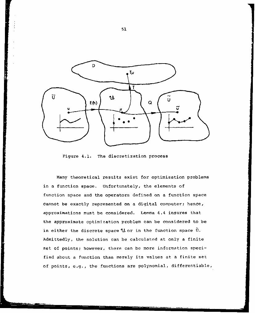
Figure 4.1. The discretization process

Many theoretical results exist for optimization problems

in a function space. Unfortunately, the elements of

function space and the operators defined on a function space

cannot be exactly represented on a digital computer; hence,

approximations must be considered. Lemma 4.4 insures that

the approximate optimization problem can be considered to be

in either the discrete space 9or in the function space U.

Admittedly, the solution can be calculated at only a finite

set of points; however, there can be more information speci-

fied about a function than merely its values at a finite set

of points, e.g., the functions are polynomial, differentiable,

52

etc. . Thus, it is felt that the elements of the subspace

give a more complete description of the approximate solution,

and solving the problem in this subspace is more in the

spirit of the original continuous problem. However, regard-

less of whether the approximate solution is considered to be

in the space 'L or in the space U, the information which is

lost due to discretization cannot be completely regained

(E1h) does not exist). Therefore, discretization error is

caused by the loss of information in the initial and

boundary conditions of the state system and in the initial

control due to the transformation E(h).

The exact gradient of J for quadratic programming

problems is given in Equation 2.30 as

g(u) = c+Au. (4.4)

Along with this exact gradient the approximate gradient

given by

4 l (4.5)

is considered. The first question to be answered is the

following. How do the approximations of discretization and

truncation (round-off is neglected) effect the calculation

of the approximate gradient .(a)?

For the purpose of illustrating how each of these

approximations enter into the calculation of r(u), consider

the following simple problem:

53

minimize

J[Ud(r, t)] 111x(rTf) I2 + .11 ud(r,t) I 2, (4.6)

subject to

Sx(r,t) = ud(r,t) , (4.7)

x(r,0) = x0 (r), (4.8)

xt(r,0) = 0, (4.9)

x(O,b) = 0, (4.10)

x(l,t) = 0, (4.11)

where TfR

I I 12 -f x2 (r,t)drdt,t2 ;r2 11' 0 f fa 00

and Tf = 4, Rf = 1. From Equations 2.23, 2.25, and 2.30 the

gradient is given by

g(u) = ud(r,t) + (S 2 Tf)] (T(Tf)x0(r)+S (Tf)Ud(rt),

(4.12)-1

where the term ?(Tf)x 0 (r) + S (Tf)Ud(r,t) represents the

forward integration of the state system from t0 to Tf, and

the second term on the right hand side of Equation 4.12 is

then given by [S I ] [x(rTf)] which represents the

backwards integration of the costate system. This explains

the reason for steps (a) and (b) in the gradient algorithm

54

given in Chapter III. In calculating the gradient on the

computer the differential operators S and S* are actually

replaced by finite-difference formulas which are truncated

approximations of S and S*. This introduces truncation

errors. Let 4 represent the finite-difference approximations

to S, and let ý(Tf)Ex 0 denote the finite-difference solution

of the homogenous state system. Then the discrete approxi-

mation of Equation 4.12 yields the approximate gradient (dis-

cretized)

-i . -i•(•J)=EgEUd+[ J(Tf)] ['(Tf)Ex+ j (Tf)Eud] . (4.13)

In Equation 4.13 discretization errors are introduced by the

approximation of the initial conditions x0 by Ex 0 and by the

approximation of the control ud by Eud; truncation errors

are introduced by the approximation of differential operators

by truncated finite-difference operators, which are repre-

-1sented by 4-1 and ý, respectively. To be consistent the order

of the interpolation formulas, represented by Q, should be the

same as the order of the finite-difference method, represented

by . Little additional accuracy can be obtained bv makina the

order of Q higher than the order of A, and if the order of Q

is lower than the order of 4, then interpolation error (see

Appendix A) is being needlessly introduced.

55

The Effects of Gradient Erroron Gradient Methods

Let Un+lG(Un 'Sn yn; Un-I ... , nu ) represent the

exact gradient iteration, then the approximations discussed

above yield what will be referred to as the approximate

gradient method U n+=G(n•nSn ; Un nl,...,n). The follow-

ing important questions arise: (1) when there are gradient

errors, do the more powerful gradient methods, such as:

the conjugate gradient method and the Davidon method,

offer advantages or disadvantages over the simpler gradient

methods?; (2) given that the convergence of the exact

gradient method is assured, under what conditions (if any) will

there result convergence of the approximate gradient methods?;

(3) if the approximate iteration does converge numerically

(in general { n at what step should the iteration

be terminated in order to insure a reasonable estimate to u*?;

(3) how is this estimate to u* made and how suboptimal is ui*?

Before answering these questions some additional nomenclature

and definitions have to be introduced. Let uaU denote the

interpolated approximation to ucU, where from Lemma 4.2 U is

a finite-dimensional subspace of U. Let R denote the discrete

approximation to J, and let I I I I represent the norm of a

vector.

56

Definition 4.1.: (61) If there exists a set S U: Sn.lNcT ri+

=n ,n>N}, then {U n is said to be numerically convergent

and S is said to be the state of numerical convergence.

Remark: Numerical convergence is different from the standard

concept of convergence. This difference is due to the finite

word length of a digital computer.

Definition 4.2.: If J[u*]=min J[u], then the optimalucU

control error IIeu11 is defined as

l ieul H :1*-u* H,

where ui*=iySNc

Definition 4.3.: The cost functional error ej is defined as

ej=IJ[u*]1- [E(h)u* ]I.

Since J[1*] cannot be computed, the cost functional error

is a measure of the suboptimality of the approximate solution.

Gradient errors have two effects on the gradient itera-

tion: (1) direction of search errors in the outer loop

iterator, and (2) linear minimization errors in the inner

loop iterator. Until more accurate finite-difference methods

are developed, it appears that the direction of search

errors must be tolerated. However, linear minimization errors

can be avoided when the effects of gradient errors on this

5 7

phase of the iteration is understood.

S[ If the exact gradient of the cost functional J[.] at

un is given by g(an ), then

g(6Un) = g(Un ) + e (Un ;h), (4.14)

where 4(W )CU is the approximate gradient at Ui, andnne (Un ;h) is the gradient orror, which as indicated depends

on the discretization parameter h of the finite-difference

method used in computing the solutions of the state and co-

state systems.

Many of the following results rely heavily on the

linearity of the dynarnicai system and on the quadratic nature

of the cost index. For a well-posed linear dynamical system,

there exists a linear transformation, given by Equation 2.18,

between the control space U and the state space X. In

addition, the discretization of a linear continuous dynamical

system results in a linear system of difference equations which

when solved yields a linear transformation between the discrete

space It and the discrete state spacer . Consequently, the

truncation error (on the nodes), which is the difference be-

tween these solutions, is also linear in the control. To be

more specific, let q(u) denote the discrete approximation of

the exact gradient g(u) calculated by the finite-difference

solution of the state and costate systems, then

58

•(u) = 6 +d1 a +aE(h)u . (4.15)

The operator 6, is linear because the difference equations

resulting from the approximation of the linear partial dif-

fcrential equations are linear.

Lemma 4.6.: If the dynamical system is linear and if J[.] is

a quadratic functional, then the truncation error in the

gradient v (u;h) is linear in u. Specifically

Sg(u;h) = ý(h)u + ag,

where 0(h)=E(h)A-1E(h) is a linear operator depending on the

discretization parameter h, and a- =E(h)c-a

Proof: The truncation error in the gradient is qiven by

4 (u;h) = E(h)g(u)- (u)

= E(h) [c+Au]-[ +dE(h)u]

= E(h)c-6+[E(h)A-kE(h)]u

= 9 + ý(h)u.

Theorem 4.1.: If the dynamical system is linear, and if J is

a quadratic functional, then the approximate gradient

is the exact gradient (apart from round-off)

of the quadratic functional

i[a]=J0 +<c,u>+ <uA>,(4.16)

59

whe re

c =QC , and . =QGE(h)

Proof: g Q 9(R)

-- [ +GE (h) u]

= + Q•.E(h)i ,

which by inspection is the gradient of J[6].

Remark: The inner product <.,-> can be calculated exactly

(apart from round-off) on the subspace U.

Theorem 4.1 is an important result because it implies

that even though 4 is not the gradient of J, org ; @ is the

exact gradient of J. Therefore, it should be possible to

at least minimize J. Hopefully, the minimum of this

approximate problem will be a satisfactory approximation to

the true solution.

The following result will be useful in the analysis of

the effects of gradient errors on the inner loop iterators.

Lemma 4.7.: Let yn be selected such that J[un +Y ns n]

< J[u 1+ysn I for all y>O, where sn is the direction of search.

Then yn minimizes J along the half-ray u n+Ys n, and is given

by<gn 'sn>

n n

in S ni As n > I(.17)

V60

Proof: Substituting un+ySn into Equation 2.21 yields,

2J[un~ ]-J[u 0 =Y<g nSn> + 2 <Sn Asn>

The first derivative of the cost change in the direction

s with respect to y is

d >

d-y(J[Un+l]-J(Un]) --- <gnSn>+ Y<Sn•ASn n

Setting the above equation equal to zero and solving for

y yields

<gn 's n>

Yn <s ,As >n n

The second derivative shows that yn yields a minimum, i.e.,

d d lu ]-J[u n) = <s ,As > > rAll 12 > 0.

By applying Lemma 4.7 it is easily shown that

Yg nn (4.18)n n

and

Y n' n (4.19)nn'

denote the control correction parameters defined by Equation

3.2 in the direction S for J and J, respectively. For dis-n

tributed parameter systems, the operators A and A are,

respectively, multiple integral and multiple summation

L

61

operators. As a consequence, Equations 4.18 and 4.19 are not

generally used in practice. Instead of Equation 4.17, the

following methods are usually utilized in the inner loop to

determine yn

1. Cubic interpolation based on functional and

directional derivative information.

2. Quadratic interpolation based on functional infor-

mation.

3. Linear gradient interpolation based on directional

derivative information (i.e., regula fa~si).

In theory these three methods yield the same result.

However, method 1 is generally considered to be superior to

the other two methods because of its rapid convergence

properties. When there exist gradient errors of sufficient

magnitude, this is not the case. In fact numerical results

indicate that when there are gradient errors then method 1 is

the least efficient of these three methods. The convergence

of the inner loop iterator is essential to the convergence

of the outer loop iterator; hence, the effects of gradient

errors on each of these three inner loop methods will be

discussed.

Method 1. Cubic interpolation based on functional and

directional derivative information

A general description of this method is presented in

(52). This method is the most sensitive of these three

' • I • i ' •I •1...... i

62

methods to gradient error because it requires a close corre-

lation between the gradient and the functional. Reliance on

both types of information (gradient and functional values)

can cause difficulties if the relative magnitude of the

gradient error is large. One reason for the difficulties en-

countered by this method is that it brackets the minimum in the

direction of search (i.e., the iterator determines two

scalars y 1 and y 2 such that yn<Yn<Yn) by determining whenSn n n-n- --

the directional derivative

S<g(un+ysn) 'Sn> (4.20)

changes sign, i.e., from negative to positive. Unfortunately

due to gradient errors, this method generally does not bracket

the minimum. This is illustrated in Figure 4.2.

n Ysn]

J +•YTS

S LOPE OF THE APPROXIMATEDIRECTIONAL DERIVATIVES

SLOPE OF THE EXACT

DIRECTIONAL DERIVATIVgS

0 0

Figure 4.2. Cubic interpolation

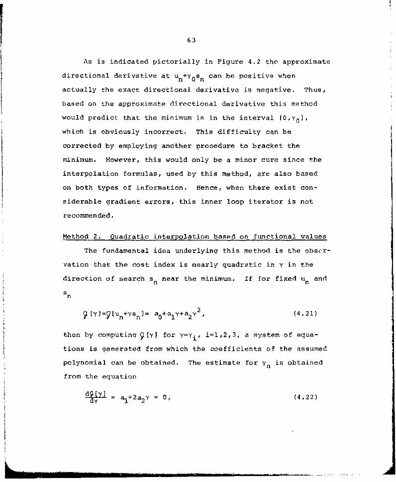
63

As is indicated pictorially in Figure 4.2 the approximate

directional derivative at Un+Y0Sn can be positive when

actually the exact directional derivative is negative. Thus,

based on the approximate directional derivative this method

would predict that the minimum is in the interval [o,y 0 ],

which is obviously incorrect. This difficulty can be

corrected by employing another procedure to bracket the

minimum. However, this would only be a minor cure since the

interpolation formulas, used by this method, are also based

on both types of information. Hence, when there exist con-

siderable gradient errors, this inner loop iterator is not

recommended.

Method 2. Quadratic interpolation based on functional values

The fundamental idea underlying this method is the obser-

vation that the cost index is nearly quadratic in y in the

direction of search sn near the minimum. If for fixed un and

s n

2[y]=9[Un+YSn]= a0 +aly+a2 Y (4.21)

then by computing 9(y] for y=yi, i=1,2,3, a system of equa-

tions is generated from which the coefficients of the assumed

polynomial can be obtained. The estimate for yn is obtained

from the equation

ad•+2a 2 Y 0, (4.22)

64

from which

Yn • .-/2a 2 . (4.23)

If 9 is quadratic then this method determines yn in one

iteration; however, if ý is not quadratic, then additional

logic is required to determine yn* The important feature of

this method is that it does not depend on the approximate

gradient vector. However, since g is not the gradient of

(g is the gradient of J), the directional derivative at the

minimum of in the direction S does not necessarily vanish;

hence, the subsequent direction of search is not a conjugate

direction and the method of expanding subspaces does not

apply. Therefore, if this inner loop iterator is used in

conjunction with a conjugate direction method, then rapid

convergence cannot be proven. Once again, it is the in-

consistency between the gradient and the functional which

causes the difficulties. Numerical experience indicates that

in the presence of gradient errors this inner loop iterator

combined with a conjugate direction method produces slow

convergence near the minimum. The slow convergence near the

minimum is caused by gradient errors which are more dominant

near the minimum (both the exact and the approximate gradients

become smaller, in the norm, near the minimum). The main

advantage of this inner loop method is that it attempts to

minimize• , which may be a better approximation to J than is

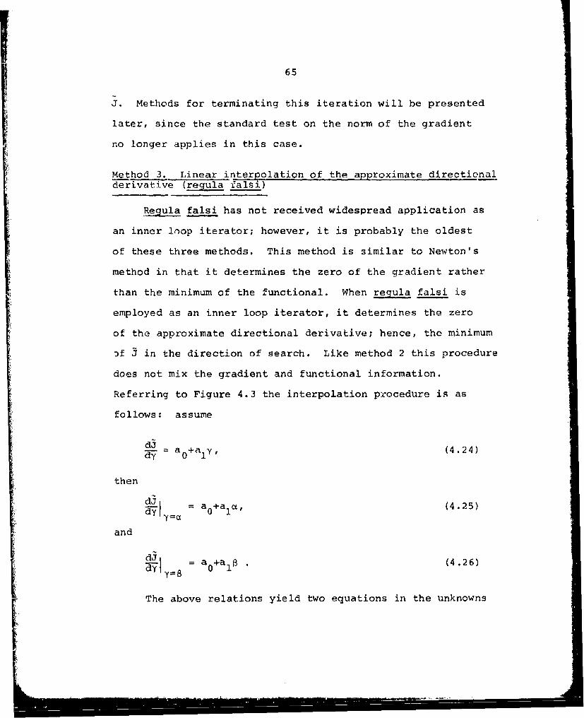
65

J. Methods for terminating this iteration will be presented

later, since the standard test on the norm of the gradient

no longer applies in this case.

Method 3. Linear interpolation of the approximate directionalderivative (regula falsi)

Reeula falsi has not received widespread application as

an inner loop iterator; however, it is probably the oldest

of these three methods. This method is similar to Newton's

method in that it determines the zero of the gradient rather

than the minimum of the functional. When regula falsi is

employed as an inner loop iterator, it determines the zero

of the approximate directional derivative; hence, the minimum

3f J in the direction of search. Like method 2 this procedure

does not mix the gradient and functional information.

Referring to Figure 4.3 the interpolation procedure is as

follows: assume

dJd a 0 +a Y1 (4.24)

then

df a +a a,(4.25)

and

i = a +a . (4.26)

The above relations yield two equations in the unknowns

66

a0 and a1 . By solving these equations for a0 and al, anapproximate expression for is obtained. The control

dJcorrectioii parameter y is determined from the zero of ,

n dwhich is given by

-adLj )/3 -W (4.27)All 8•y~ dy y=8 y= Y--S

THE LINEARAPPROXIMATION OF [dii

dJddYY

THE APPROXIMATEDIRECTIONAL DERIVATIVE dJ

dJ• ] dy

Figure 4.3. The regula falsi iterator

67

Lemma 4.8.: If J is a quadratic functional, then the regula

falsi method determines n such that

J[Un +ýn n]_ J[un +Yn I for all y>O.

Proof: For simplicity let a=O, then Equation 4.27 yields

Yn = (<nn n n >)/(<nn'n>-<4(Un+Sgn)'gn>)

= (<4,n n>8)/(<4n n n -BA( n+•n n>)

= (<4n ' n>)/(<n ' n>-<4 n +BAsn n >)

= -<gn',sn>/(SnASn>,=<n 'gn >/9n A n >

and the proof then follows from Lemma 4.7.

Thus, the regula falsi method is a numerical procedure

for obtaining the result of Equation 4.19.

Theorem 4.2.: If A is a self-adjoint operator, if the con-

ditions of Theorem 4.1 are satisfied, and if the regula

falsi method is used in the inner loop, then the gradient

iteration Un+l=G(UnSnyn; Un-l,.oUn-m) generates a

sequence {u n} which numerically converges to the approximate

minimizing element in U, specifically

[uA] = amin J[u] .

[ 1U

68

Remark: The standard convergence proofs for these three

gradient methods can be applied to Theorem 4.2 (refer to the

references given in Chapter III).

Corollary 4.1.: If the conditions of Theorem 4.2 are satis-

fied then both the conjugate gradient method and the Davidon

method converge in a finite number of iterations to the

minimum of J.

Proof: The proof follows from the fact that U is a finite-

dimensional subspace of U, and from the application of the

results contained in (41) and (50).

Theorem 4.2 is significant, since it implies that {( n

generated by G minimizes J and not J nor . Corollary 4.1 is

important, since it insures convergence of the conjugate

gradient method and the Davidon method in a finite number

of iterations.

Error Estimates

Since {•n} does not minimize J, it is desirable to com-n

pute the optimal control error. This, however, is impossible

without prior knowledge of the solution u*. Nevertheless,

estimates of the optimal control error may be obtained by

means of the results given below.

69

Lemma 4.9.: Let V J denote the gradient of a positiveu

definite quadratic functional J defined on a real Hilbert

space U, and generated by a self-adjoint operator A, then:

(W) Jg IuJ j2=llg(u)112 is also a quadratic

functional with Hessian 2AA,

(ii) The set defined by Sg={U: llg(u) I12 =c} is a

hyperellipsoid in the Hilbert space U. and,

(iii) If J [u* ]=min J [u], then u*=u*.g g ucU g g

Proof: (i) J [u]=fjg(u)jj 2 =<qg>=<c+Au, c+Au>g

= <c,c>+2<c,Au>+<Au,Au>.

Since A=A*, it follows that <Au,Au>=<u,A*Au>=<u,AAu>.1

Thus, J [u]=<c,c>+2<c,Au>+ 1<u,2AAu>, and the Hessian is then

2AA.

(ii) J is quadratic from (i).g

(iii) V uJ g=2Ac+2AAu; hence, VuJg = 0 implies that AAu=-Ac-1 -1 - L

and that u*=-A A Ac=-A c=u*.

Lemma 4.10.: Consider the translation defined by 6=u-u*,

where U[u]=J[u]. Then:

(i) J[i^]=J[U*]+ 1<Q,Al>.

(ii) V iff]=VuJ

I I I I I I ' ' ' . .. . .

70

Proof: (i) JS[a]=J[u]=J [u+u*]

= +<c'u+u*> + 2"

Expanding and using the representation of the solution

U*=

yields

J[ u]=J 0 - T-<C,A C> + L U,A&.

Now it is easily shown that

J[u*]=J +<c,u,> + l<U*,Au,>02 -(,A +1 -i -l

=J 0- <c,A-I> + VA c,AA c>1 -

J- 0 <Cc,A->

and thus,

J[6]=Jtu*] + 1 iU,>

(ii) VQ?=AU=A(u-u*)=Au-Au*=Au-A(-A1)4

=AU+C=V J.U

Theorem 4.3.: The vectors defined by I u 2=ax2 12I

and 1U11 =mIin}IaII are eigenvectors of A (i.e., AA) withueS~

2 2eigenvalues MA and mA, respectively.A A

71

Proof: By using a Lagrange multiplier X the proof of this

theorem can be formulated as an optimization problem, i.e.,

extremize subject to the constraint S This

constrained problem can be reformulated as an unconstrained

problem by considering the functional

f[,pi,]=l II I + X (c-I1A11A II

Then, the gradient of f is given by

af 2- [CIAI 2a

I [•,a] 12

where differentiation is in the Fre6het sense.

By setting Vf=O, one obtains

2ý 1

Therefore, the vectors au and fi which extremize 11all2

subject to the constraint Sq are eigenvectors of A. Since,

M and mA are spectral bounds for A, it follows that MA2A MA

2 2 2and m are spectral bounds for A (since, A eAAe=AXeXAe

=Xle=X2 e).

Theorem 4.4.: Let ljg(ýL 112 denote the exact normed gradient

squared of J[.] at Z. Then,

Ai mA ll g(N)1lMA mA

72

Proof: Let u=6,-u* and note that since A is self-adjoint, so isAA. By Lemma 4.10, [ lg(ýN)l 2=l A((j)ll2=l IA61 12=<aA 23>. Thus

from Theorem 4.3,

2 2 M2110I112'mAII611I < <1a,•A>

and

21 1C1 2 < 2 2< M jI 2

mA gA < M

which yields the desired result after taking the square root

of

214(uN 2 <I I g (UN) 112

2 < I2I- 2

MA mA

From Theorem 4.2, {Un} minimizes J; hence, {4(Un)})-0. This

resuics in a method by means of which lIg(i) ll can be esti-

mated.

Theorem 4.5.: In the state of numerical convergence (see

Definition 4.1), the alpproximate gradient methods re-

sented by un+l=G( nsn ; u n-l''un-m ) with

y =- <,S n>/<Sn,An -, insure that g(uN)=0. Thus,Yn= nP n n' nN

I lg(N) 11=1 leg(uN;h) ll

Proof: From Equation 4.14 g(Un )-g(Un)+e(6n ;h). Now n

minimizes J (Theorem 4.2) which implies that f(g(n))-+0 with n.

73

Thus g( =)e 9(u ;h) for all n>_N.

Combining Theorems 4.4 and 4.5 an estimate of the optimal

control error is obtained by means of the following

Corollary.

Corollary 4.2: Let eg (i;h) be the gradient error at the Nth

iteration of n+=G[6n , nyn ; ii nl,..,U n1m. Then the

estimate

lie gN ;h)ll/MA.< I fA*-u*ll < Ile 01N h)ll/m.,

is obtained

Proof: The proof follows immediately from Theorems 4.4 and 4.5.

Unfortunately, only the projection of the gradient error on

the subspace of interpolating functions can be obtained on

the computer. Let Pe cU be the projection of e cU on the

subspace U, and let 01 denote the annihilator of U. From

the Projection Theorem, (refer to Appendix A) the gradient

error is given by

eg(u ;h) = Peg + Y, (4.28)

where YEtV. From the triangle inequality it follows that

Ileg,(6 n h)Jl i < lPe 1 + Hly , (4.29)

and the estimate

I74

I u*u*I _< (I IPe 1l1 + II I Y )/mA (4.30)

holds.

From tne Projection Theorem, fj+O±=U, and Thus, as the

dimensionality of 0 increases (refinement of the d'screti-

zation) the quantity I YJ 1+0. Equation 4.30 yields a

practical method by means of which the optimal control error

can be estimated.

If method 2 is utilized in the inner loop iteration then

{g(Un)}/O, and thus, another method for estimating

I Ig(iM)J is requ red. Let ýn be the control correction

parameter for 9[p) in the direction Sng Since, method 2

minimizes L[il] in this direction, 9n is then given by

<Qg nQEn >Yn = n (4.31)

<QEn ,QdESn >

If the steepest descent method is employed, or if the other

gradient methods are restarted each time an up-hill direction

of search occurs, then Sn 0. As noted before this inadvertent-

ly creates a fixed point for the iteration, without causingthe gradient to vanish. In addition, since yn eventually

becomes small, slow convergence results. This properf-y has

been noted in numerical results (57). Termination of the

iteration occurs when

<QEg ,QEg > 0. (4.32)n n

- n-lU

75

This implies that

<QE(j n+e )g Q~i > =(4. 33)

and since QEg n=g n, Equation 4.33 yields

<9 'gn n<~ gn>(.4

Now consider the relations,

IIQEg '112 = OEg, iQEgn> = <QE (4n+e ),oE(4 +e )>

<4 +QEe 9 4 +QEe 9>

4IInII +2<4 n QEeg9>+HIQEegII2 (4.35)

Substitution of Equation 4.34 into Equation 4.35 yields

IIQEg n 12=1 IQEe 9I12 _11 nI 112. (4. 36)

Using the Projection Theorem and the triangle inequality one

obtains the estimate

lIgn 11 < JIQEg nJI + HI11, YCOL . (4.37)

Thus, the estimate1

*11 [I IQEeg91 2_11i 112]f+)2I (.8

is obtained for the case where method 2 is used as the

inner loop iterator.

An estimate of the cost functional error can also be

given in terms of the gradient error and the spectral bounds.

76

Theorem 4.6: Let J be a quadratic functional defined on U

generated by a self-adjoint operator A and by an inner

product <.,.> . Let J be the approximation of J

defined on the subspace U generated by A and by the inner

product (.,.) . Then

Ij~u~-a[U 1 2.e + -111*1*1 [Ieq11+1eIIeIU +1 2 p

+ l~llci~ llecll lle11 } l le {

gA

where J= J 4- eJ0, c=C+ec and <.,.>=(.,.)+e0 p

Proof: Let

J[u*]=J +<c,u*> + l<u*,Au*>0 2

and•[•j*]= 0+16,iu.1 + I(jj j*

o 2The relation

1 ,1 21-ý,u*,Au*> = <q(u*) ,u*> - <u*,c>,

implies that

J[u*]=J + T< ,u*> + -<u*,g(u*)>

I1

=J 0 + <6+e ,u*+(u*-uj*)> + -<u*,g(u*)>2 c 2

Expanding the above equation, takilig into account the errors

due to the approximate inner products, and taking the absolute

value, yields the estimate

• -N• 1 . . . . • . . . . .• . . , , , , , , , • : , • . .

77

IJ[u*]-.[i *]l < IeJ01 +e + I,u* -1 *>< +1 1 +i 2

+ I I<e ,u*-a*>l + lle 1I + 1" le 2

p p

+ 1 I<u*-a *,g(u*)>l + 1<.i*,ej.

Using Schwarz's inequality and Corollary 4.2, and by grouping

terms properly the desired estimate is obtained.

In practice a[Eu] is computed rather than J[i]; however,

IJ[u*P-?[E6*jl < IJ[u*]-3Vl*]l + le l, (4.39)

where

e.= i [i]-EiC].

The error e- can be eliminated (apart from round-off) by

the proper selection of the quaradure formulas. For example,

if piecewise quadratic interpolation is employed to determine

function values between the node points, then the use of

Simpson's quadrature formula over each partition insures that

ea=0.

Determination of the Parameters in theError Estimates

The estimates of the optimal control error and the cost

functional error are based on the gradient errors and on

the spectral bounds mA and MA. Hence, in order to use these

estimates methods for obtaining these quantities are required.

I

78

Gradient error

At the present time two methods have been utilized for

estimating lie eg: (1) error bounds in terms of higherg

order difference, and (2) asymptotic extrapolation. Since

the first method is problem dependent and also conservative

only the second method will be discussed here.

Asymptotic extrapolation is an attempt to actually com-

pute the gradient error. It is based on the fact that if the

approximation to the gradient is of order P, then

g N+ = . hPeg (Z) + *(iiN;hP+ 1 ), (4.40)

where e is defined as the magnified error function.gi

Solving for the gradient j(uN) by using stepsizes of h and

qh, respectively, O<a<l, two equations in g() and (N)

result, which when solved yield

Ile 9 0 N :h) j = [l/(l-hP)]jIIý(dN;qh) -ý(N;h) I. (4.41)

In view of Theorem 4.2, 4(ua ,h)=O, and thus, the estimate

l ieg(UN;h)II = [l/(l-hP)]j j4i (N qh) ll (4.42)

for the norm of the gradient error is obtained.

For the class of problems considered the lower spectral

bound mA can be determined analytically. The general form

of the Hessian operator for this class of problems is

A ac + T*T. (4.43)

79

By Lemma A-i, T*T is self-adjoint with a lower spectral bound

of zero. In addition from Lemma A-2, a+T*T is also self-

adjoint with mA=ct. This analytical result is certainly an

advantage in performing the error analysis on quadratic

programming problems. However, in many cases it is not

possible to determine analytically either the Hessian operator

A, or its spectral bounds. For example, in non-linear

problems the operator A does not appear. However, if the

quadratic approximation is valid near the minimum of a non-

quadratic functional (which is at least convex), then Davidon's

method presents a numerical procedure by means of which an

approximate Hessian and its spectral bounds can be obtained.

Theorem 5.7.,: (50) Let A be a Hessian operator defined on a

real separable Hilbert space U. Then there exists a subspace

Ur-1 such that

n, -i.Hu = A u as n÷oo,

for all ucU, where {H n is the Davidon deflection operator

defined by Equations 3.11 through 3.16.

Corollary 4.3.- Let 1IHn ul-HUn I<E for all n>N, and let

mHN and M N denote the smallest and the largest eigenvalues of

H N respectively. Then

mA l/MNH

I~~ ~ H . .

80

and

MA H/m.

N N NProof: HNA= I implies that MHmA 1 mH MA'

Unfortunately, Mn rather than Hn is obtained on the computer,

where RnAKI.I Thus, the previous error estimates are valid

only in those cases where mASmA=i/MV . If mA decreases under

a refinement of the mesh, then one might possibly consider

using mý in the error analysis. However, this would probably

produce a more conservative error estimate.

Geometric Interpretation of theError Bounds

Due to gradient errors, one should not expect to obtain

the true solution of an optimization problem when gradient

methods are employed. Thus, estimation of the errors

become an important part of the solution. The error esti-

mates presented in this chapter rely heavily on the quadratic

properties of the cost index. These estimates are based upon

the following geometrical considerations. Assume a gradient

method is employed which ensures the vanishina of the approxi-

thmate gradient. Then the true gradient at the N iteration

becomus equal to the gradient error. Obviously, if the

gradient error can be calculated, then it is possible to

iAssuming that method 3 is used in the inner loop.

81

cont inu•u Lho i te rat ion. ][ow Vo, r, in reonora1 it is much

easier to estimate the norm of the qradient error than the

gradient error itself. If only the norm of the gradient error

is known, then it is impossible to continue the iteration

because of the lack of a direction in which to proceed.

Now assume that Ifle ff can be computed. From Lemma 4.9, the

set S c=u: llgl-2=c} is a hyperellipsoid, which if

orientated properly would have its center at u*. However,

since only I gjl can be estimated, it is not possible to

determine this direction. Nevertheless, the true solution u*

must be contained in a hypersphere which has a radius equal

to the semi-major axis of the constant gradient (at U

hyperellipsoids. These considerations are illusted in Figure

4.4.

LOCUS OF THE CENTERSOF THE CONSTANTGRADIENT MAGNITUDE

CONSTANT GRADIENT CONTOURSMAGNITUDE E LLIPSOIPES

\ I

Figure 4.4. Geometrical interpretation of the oprimalcontrol error

82

If the ratio MAimA is large, then these error estimates be-

V come conservative. In theory an inner hypersphere can be

constructed based on the minor axis of these hyperellipsoids.

However, the methods used in estimating the parameters in these

error estimates makes these lower bounds questionable. It isworthwhile to note that the constant J contours are in general

translated and deformed because of gradient error. This is

illustrated in Figure 4.5. The fact that the approximate

gradient algorithms only solve the problem in a subspace U

of U is illustrated in Figure 4.6.

J = C PROJECTED jrONTOU

Figure 4.5. Constant cost contours

R 3

J C CONTOURS IN THE

ORIGINAL CONTROL SPACE U

Figure 4.6. Minimization on a subspace

84

CHAPTER V. NUMERICAL RESULTS

All computations reported in this dissertation were per-

formed on the IBM 360 Model 65 digital computer usinq the

Fortran IV language with double-precision arithmetic. Compu-

tation times quoted are the time used by the Central Proces-

sing Unit (CPU) during program execution. Although the

Central Processing Unit time is the best measure of the

computing effort required, it is not precisely reproducible

on identical programs due to the multi-programming feature of

the system. Storage requirements reported are in terms of

array area used in BYTES, which does not include object code

storage requirements.

The solution of the state and costate partial differential

equations were performed with a standard second order

symmetric finite-difference algorithm (62). The multiple

quadrature algorithm used in computing the cost functional

and the inner products was based on the Gauss-Legendre ten

point quadrature formula (53). Piecewise continuous quadratic

polynomials were used to obtain function values between thenode points. All three types of inner loop iterators

described in Chapter IV were employed; however, only the

results obtained with method 3 are presented. Numerical re-

sults for the modified conjugate gradient method, the

Davidon method, and the standard "best step" steepest descent

method are presented and compared in Example 5.1. Since the

85

conjugate gradient method proved superior in terms of CPU

time (hence less computer costs) it was utilized on Examples

5.2 and 5.3. In Examples 5.2 the constrained distributed

control problem is considered. Ekample 5.3 presents results

for the boundary control problem. The three-dimensional

figures presented were generated by the Cal-Comp Digital

Incremental Plotter with a subroutine developed by the Iowa

State University Computation Center.

Example 5.1.: The unconstrained distributed control of the

vibrating string

The unconstrained, fixed time, penalized, minimum energy

distributed control of the vibrating string is considered.

The problem may be stated as follows:

minimize:

Ju iF x2 R)dr + U d 2 (r,t)drdt, (5.1)J[d]•0 rfd+ 0 •0

subject to:

Sx (r,t) =ud (r, t), x(r,t) (5.2x(r)

x(r,o)=x0 (r),

X (r,0)=0,r

x(O't)=O, Figure 5.1. The vibrating string

x(l,t)=0,

22 2where = 2 x0 (r)=sin~rr, a=2, B=0.5, RF=1, andt2 r2 0 F

T F=4. The initial and the boundary conditions are illustrated

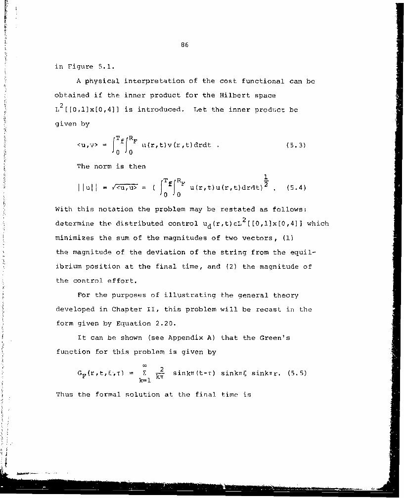
[i86

in Figure 5.1.

A physical interpretation of the cost functional can be

obtained if the inner product for the Hilbert space

2L [[0,lx[0,4]] is introduced. Let the inner product be

given by

<uTffR=u(r,t)v(r,t)drdt (5.3)

The norm is then

_~ (T!F 2.Ill- RF u(r,t.)u(r,t)drdt)' (5.4)u l ul -- U -- fo

With this notation the problem may be restated as follows:

determine the distributed control ud(r,t)L2O[[0,l]x[0,4]] which

minimizes the sum of the magnitudes of two vectors, (1)

the magnitude of the deviation of the string from the equil-

ibrium position at the final time, and (2) the magnitude of

the control effort.

For the purposes of illustrating the general theory

developed in Chapter II, this problem will be recast in the

form given by Equation 2.20.

It can be shown (see Appendix A) that the Green's

function for this problem is given by

G= 2 sinkTr(t-T) sinknr sinkrr. (5.5)F k'~

Thus the formal solution at the final time is

4.,

87

TR

+{ff~f G(r, Tf, ~d~ -r) drd-, (5.6)

which according to the notation developed in Chapter 11

becomes

x(rT f = PITf)x 0 + S(T f )u do (5.7)4

and as a result the cost index is then

J~ud = j1I I(T )x0 + + )uu~ 1 (5.8)

by expanding Equation 5.8 in terms of the inner product, and

by employing the definition of the adjoint operator

(<Sx,y>=<x,S*y>) Equation 5.1 becom~es

J[u l=J +.<ctU > + I udAd> (5.9)

where

1= ((. 100 Tf II(f~xI

f

an2aST i- [S (T 4)(T [ST)l 5.1

f

Substitution of (3.5, a=2, and T f=4 into Equation 5.12

yields

86

in Figure 5.1.

A physical interpretation of the cost functional can be

obtained if the inner product for the Hilbert space

L 2[[O,llx[0,4]J is introduced. Let the inner product be

given by

<UV IT f RF= u(r,t)v(r,t)drdt (5.3)

The norm is then1

lull = V 7u>= ( fF u(r,t)u(r,t)drdt) 2 . (5.4)f0 •0

With this notation the problem may be restated as follows:

2determine the distributed control ud(r,t)eL [[0,1]x[0,4)] which

minimizes the sum of the magnitudes of two vectors, (1)

the magnitude of the deviation of the string from the equil-

ibrium position at the final time, and (2) the magnitude of

the control effort.

For the purposes of illustrating the general theory

developed in Chapter II, this problem will be recast in the

form given by Equation 2.20.

It can be shown (see Appendix A) that the Green's

function for this problem is given by

0O

GF(r,t,&,T) = 2 sinknf*(t-T) sinkrF, sinkerr. (5.5)k=-i

Thus the formal solution at the final time is

87

x(rTf) = {RF G(r,T;,t0)x()d

+ JTff G (rTf,ý,T)UdCI(ý,)d~d', (5.6)0 0

which according to the notation developed in Chapter II

becomes

x(rTf) = I(Tf)x0 + S- Tf)ud (5.7)4

and as a result the cost index is then

J[ud) -= l(Tf)x 0 + S-Tf )ud 12 + I 12 (5.8)

By expanding Equation 5.8 in terms of the inner product, and

by employing the definition of the adjoint operator

(<-Sx,y>=<x,S*y>) Equation 5.1 becomes

J[ud]=J0+<CUd> + 2Ud,AUd>, (5.9)

where

0o T (P Ul (Tf)xo1 2I (5.10)

2ct -1i 5.1

2-a[S (Tf)] (Tf)x0, (5.11)f

and

A 2 + -[S (Tf)] [S (Tf) . (5.12)f ff

Substitution of a=.5, a=2, and T f= 4 into Equation 5.12

yields

88

A = 1 + [SITf) [SITf)], (5.13)

and thus by Lemma A-5, mA=l. The gradient of J is given by

g(u) = c + Au

= (S(T f)(Tf)X0 + [l+[S (Tf)] [S1 .Tf)J]]udS-i * -1

= ua+[S (Tf)] [c(DTf)x 0 +S (Tf)ud] (5.14)

= Ud+[S -Tf)*[x(r,Tf]

= Ud+[ (Tf)] [4x(r,Tf)].

Equation 5.6 could be used to compute the cost index and

Equation 5.14 could be employed to compute the gradient;

however, a brief numerical study of the convergence of the

series in Equation 5.5 indicated that a finite-difference

method is much more efficient.

A summary of the defining equations and their discrete

approximations is given in Table 5.1.

The results of the solution of this problem by the con-

jugate gradient method (modified), the steepest descent method,

and the Davidon method are presented in Table 5.2. These re-

sults indicate that for this problem the convergence of the

Davidon method is superior to the other two methods. In

addition it is apparent from Table 5.2 that both of the

second generation methods offer a substantial improvement

over the standard "best step" steepest descent method. This

can be seen by comparing the approximate gradient magnitudes

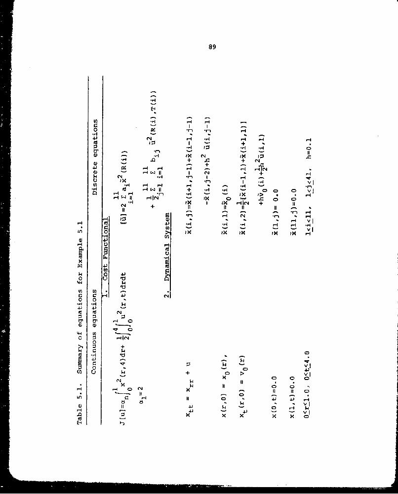
89

I *- +

+ .4 +N

1.4 PN r1 I H -qjlr- " 11 1 *.4 1

In -'4 H -A s - ..

.r (dI + -4 +*.f-r4 0 0 0 D vJr-H H r*4 '' ) X >H-Hr-4 I Hr *- IX 0 * . 0 C)

IX I ix HIN1C. + I+ I I it I -

r- Hj N- -r H* to ~ - - vL) 0X IX I X iX IX H4-I

U

0 4.)

4.4

o 0

01 01 0

) 0)wQ D

4.4v I0 4

5. 14C) C

ý44v

41 1 -4 - C)VH4-J '- 4-1

x x X X0

r 90

0 H1

En

-7 4

41- 104

C r- 4I 0 t

44I t44 C

0 -d 0f-, 0 -

ci -- (N .0

a) 0 +4 +-::I -' - -.4 '.

r.) "W 04

H. +4fl -

r. 4-) C40 00

C C;

r4 '1

00

1' 91M 0 Hr-I

-W A -4 r H-4 i -II E:X X X X X X X uw

tr?m r-~ f f- r- 1- M CO J-

,~ V H (14 % '0 Nq N1 N 40 .1-

(4m 0 0 0 0 0 4)

HHHr-4 r H - r- 4 - a0)x x x x XX -XX dt7 4-4

g -L 0~., 4 -~ 4 H .4J 0CO

q4 ~ D N :) 0O>~j (%J 1H H 04J H4.3

r-4HN V 00

o a0 0 0 0 0. CDH r 4 H H H H- - -~ U) t-If

4-) A x XX X x x x x x x fu z: >1 0C -r-e r- M. 0 U. EV If r

.1) OD -W C)4 4 --I N* - (N N r- CD~~~~ 0~NN V H rfU'O V 04) (

4) . . .* . HP4 0 . HNf 5CD 0 10 C)C000H'.0 .I -4 x - * Ln

q) (N 4J0 H -H) HH 000 a0 NI ( -4 0. )

40 o o o 0 ) 0 0 11 9 X -w ..4H 1-4r-4H-Ir-4 HH4H-1r- -4 r4 ) in4~ M

.41 4 X XX XX XX -P4 0 4-) W 0W 1N Mi N0( 0H 'VN tn4J CO Hf-4 (H 0M) '..0 %0 Ln C-4 N :D 0 5-) IM H' 0 0 g

OD 0 0 0 0 0O OD0 0 0 (n M VI a .,.1 0

00 M5 1) 4JH V FOU 4) LAF- r4 P- E 4-4 0

*0 (V~-~ H .4 v4c 0 54 4)50 4-'*Ln~ c N I IV 10 I r- 0 0 9

4)4) HHHHHH0 0 0- : W~S f $4J (4-45 0) )(L) X X Xl X X X XX I- H '.04 f L 4J-~ ý4 W -

x N NN x xl x (L)', -r 0j) *

x W g r- M '.oM 4rnv M a 014' - ) * , )W0-4 0) -4 e V)t-3raIr- 3t w4 ~ *d ) M4 ý4

coi C-) a) o o o oco .4-) .>4 k. 4)05 wH . C 00 co w) 0'44 r-4 r-4 0 0 0 0 0Q0 0'.) $4- $4i 54 H4 4) ly

C) ) C0a0 00 C 'rN 0 0 0 ' O11 (IN n 0 -H 4.in Q) P-4 P H4r H4F-HH r -4 -Ii NI r" 54 k 0 Mc -,4 4.4.S4j . XX9 4X X XX X X 4) 11 -$.i54- 0OC)(hJIJ 41)H- AS C: t (7NoD w Ln Ln Ln Ln E ) ) -0 Lf). %D M4-) C~

m 1 a C %D r4 -4 1 H- -IH H-A MH r-4 U 4j ~ 4.)0 - V ~%D "N N N N CN 4-)(0 **H- x *- Ji . 11I4) t e ý4 Cm- 1 H. -4H H 54 U)I 0 cUo ii to (D 11 0fl

00cc OD 0c 00COco 00 D0 H-- 1494 R) -4 41)0 . I a, * 4.J M 4- 0 n 11 4) 04-4

u n > r. 3 7 -H M 3U pq H4 0 V1- 4J(V 0

(U44 -4 tr (

4J )C 44 )- (H4 14 a N- N M U DN r- H 4J W

E4H Mwv -

92

(columns 2, 4, and 6 of Table 5.2) at each iteration. However,

the Davidon method required in excess of 150% more CPU time,

than the modified conjugate gradient method. In add..cion the

Davidon method required 200% more array storage than did the

modified conjugate gradient method. Thus, at least for this

problem the modified conjugate gradient method appears to be

the most efficient of these three methods with respect to

computer run-time and storage requirements. In large practical

problems the run-time and storage benefits of the modified

conjugate gradient method would become an even greater

advantage of the method. Since each inner product calculation

is essentially a double numerical quadrature, the excessive

CPU times of the Davidon[q] method can probably be attributed

to the large number of inner products required by the

algorithm. However, it might be possible, it extreme care

is taken in programming, to make the Davidon[q] method

competitive (with respect to storage and CPU time) with the

modified conjugate gradient method.

The results presented in columns 1 and 5 of Table 5.2

indicate that the discrete approximation of the cost function-

al J[.] given by 9 [.] does not decrease monotonically, as the

conventional optimization theory predicts, but rather

increases after the third or fourth iteration. This apparent

contradiction is explained by the approximation theory

developed in Chapter IV, which showed that the numerical

i

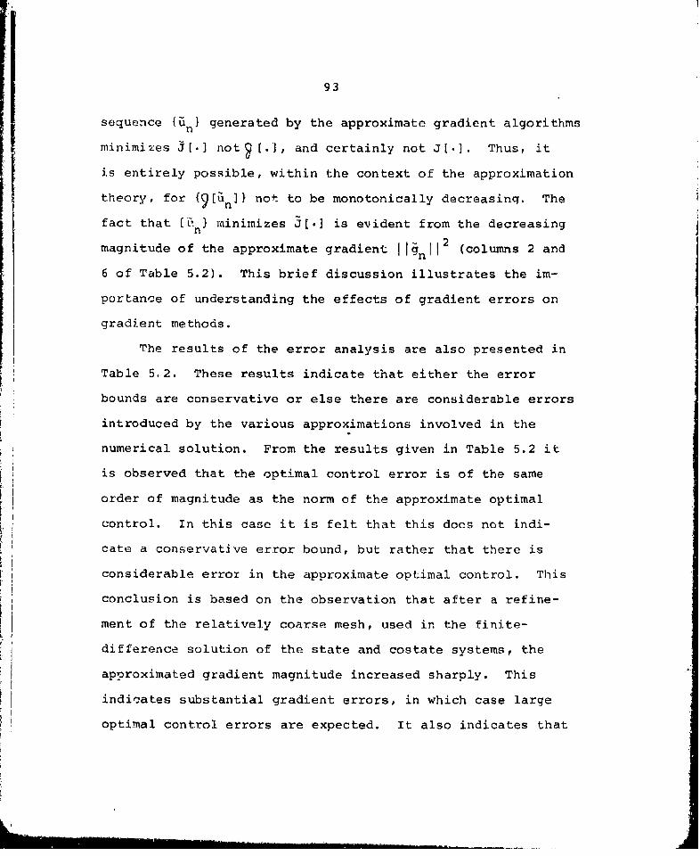
93

sequence {Zirn) generated by the approximate gradient algorithms

minimizes j[.] not ?[.1, and certainly not J[.]. Thus, it

is entirely possible, within the context of the approximation

theory, for f9[Un]} not to be monotonically decreasinq. The

fact that [an ) minimizes d[.] is evident from the decreasing

magnitude of the approximate gradient 1 lnn112 (columns 2 and

6 of Table 5.2). This brief discussion illustrates the im-

portance of understanding the effects of gradient errors on

gradient methods.

The results of the error analysis are also presented in

Table 5,2. These results indicate that either the error

bounds are conservative or else there are considerable errors

introduced by the various approximations involved in the

numerical solution. From the results given in Table 5.2 it

is observed that the optimal control error is of the same

order of magnitude as the norm of the approximate optimal

control. In this case it is felt that this does not indi-

cate a conservative error bound, but rather that there is

considerable error in the approximate optimal control. This

conclusion is based on the observation that after a refine-

ment of the relatively coarse mesh, used in the finite-

difference solution of the state and costate systems, the

approximated gradient magnitude increased sharply. This

indicates substantial gradient errors, in which case large

optimal control errors are expected. It also indicates that

94

for this problem piecewise quadratic functions may not be

the best selection for the interpolating functions. Piece-

wise linear approximating functions were tried but as ex-

pected gave even larger estimated control errors. Due to the

nature of this particular problem, trigonometric approximating

functionswould be the obvious logical choice. A discussion

of this consideration will be deferred until the other examples

are considered.

The cost functional error estimate is obviously con-

servative. This of course can be explained by the methods

used in deriving this estimate (i.e., the triangle in-

equality, Schwartz's inequality, etc.).

The initial guessed distributed control, the initial

trajectory Uist component), the numerically converged approxi-

mate optimal control, and the corresponding optimal trajectory

are depicted in Figure 5.2, (a), (b), (c), and (d), respective-

ly.

Example 5.2.: The constrained distributed control of the

vibrating string

The constrained, fixed time, fixed terminal state

(partial), minimum energy distributed control of the vibrating

string is considered. The problem may be stated as follows:

minimize

J[ud]=f3 Jff:F u (r,t)drdt, (5.15)0 0 d

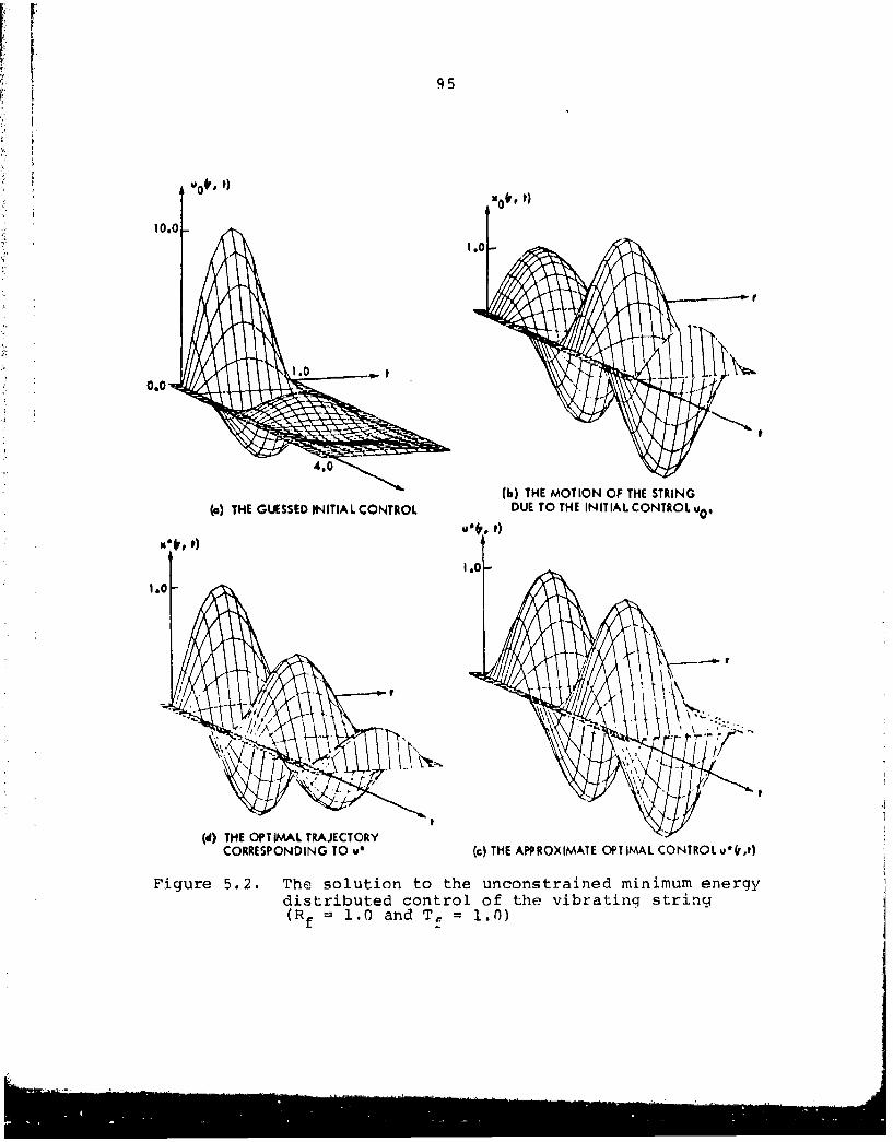
95

u 0 4OO, 0

10.0

(b) THE MOTION OF THE STRING()THE GUESSED INITIALCONTROL DUE TO THE INITIAL CONTROL U0 4

tt

(d) THE OPTIMAL TRAJECTORYCORRESPONDING TO we (c) THE APPROXIMATE OPTIMAL CONTROL 00r,t)

Figure 5.2. The solution to the unconstrained minimum energydistributed control of the vibrating string(R f = 1.0 and T f =1

96

subject to

Sx (r't) =Ud rt (r,t), (5.16)

x(r,O)=x0 (r) , x (r, 0)

x(r,Tf )=O, Ix, T

xt (rO)=O,

x(Ot)=O, Figure 5.3. The vibrating string

x(l,t)=O,

a2 22where S = -a , x 0 (r)=sinnr, a=2, 6=0.5, RF=l, and Tf=4 .t2 7r2 0f

at ar

The initial, final, and boundary conditions are illustrated

in Figure 5.3. The primary difference between this example

and the previous one is that in this case the terminal con-

dition x(rTf)=O is included. Since this terminal constraint

coupled with the dynamical system constitutes a constraint

in the control space U, this problem is not directly solvable

by the gradient methods. Thus the penalty function method is

employed to alter the form of the problem by replacing the

constrained problem by an approximate unconstrained problem.

The introduction of the penalty function to account for the

terminal constraint yields a new cost functional

JF x 2 (r,Tf)dr + J[ud], (5.17)Jp[Ud]=cn JO0 d

where the penalty constant an is arbitrarily chosen. The

defining equations and their discrete approximations are then

exactly the same as in Example 5.1, and are given in Table

5.1. The Sequential Unconstrained Minimization Procedure is

97

to solve a sequence of unconstrained problems which converge

to the solution of the constrained problem.

Results of the solutions by the modified conjugate

gradient method with increasing penalty constants an are

presented in Table 5.3. The initial guessed control, the

initial trajectory, the numerically converged approximate

optimal control, and the corresponding optimal trajectory

for a n=100 are depicted in Figure 5.4, (a), (b), (c), and (d).

The results of the iteration resulting in Figure 5.4 are

given in Table 5.4. From the results presented in Tables

5.3 and 5.4, and from the solution illustrated in Figure 5.4,

it appears that the penalty function method offers a practical

means for solving constrained problems of this type.

Table 5.3. Penalty constants for the solution of the con-strained vibrating string problem

Penalty Constant IJ=J -P[x ConstraintW p Error

2 0.24954254xi0 0 0.14859240xi0 0

5 0.55010654x10 0 0.52410559xi0-1

1250 0.10938682xi0 0.10421661x0- 2

100 0.11454726xi0 0.27283289xi0- 3

500 0.11894317xi0 0.11353210x0-4

1000 0.11957950x101 0.28465427xi0- 5

98

0oS X) 0( t)

10.0

0. 0

•l4.0

m) THE INITIAL GUESSED CONTROL (b) THE INITIAL STATE TRAJECTOR,

u00, t)

0.0 --. 0

Cc) THE APPROXIMATE OPTIMAL CONTROL (d) THE OPTIMAL TRAACTORY

Figure 5.4. The constrained minimum energy distributed controlof the vibrating string, an = 100

99

Table 5.4. The solution of the constrained vibrating stringproblem

Iteration Modified Conjugate Gradient Methodnumber G4[n] <j 'gn >

0 0.35919006xl0 2 0.24209658x10 4

1 0.76073334xi0 1 0.12886314xl0 2

2 0.11789181xi0 1 0.52546089x10 0

3 0.i1727328xl0 1 0.22517444xi0- 4

4 0.11727398x101 0.21432484x10- 3

5 0.11727564x10 1 0.45933457x10- 6

6 0.11727565x10I 0.55115803xl08

7 0.11727560xi01 0.16968429xi0 7

8 0.11727560xi0 1 0.17853686x0- 11

9 0.11727559x10 1 0.44314448xi0-12

10 0.11727559xi01 0.30146695xi0 1 2

11 0.11727559x101 0.14755488xi0- 1 5

CPU Time=52.6 sec (with plot)

Storage = 140K Total (ARRAY + OBJECT CODE)

u 0 (r,t)=10e- t sinwr cosvt.

While performing the numerical study of the effects of

the penalty constant on the solution, it was discovered that

by guessing the initial control to be identically zero (i.e.,

u0 (r,t)=0) the conjugate gradient method converged numerically

in exactly one iteration. The results of the iteration for

the case where a n=5, x(r,0)=sin7rr, and u 0(r,t)=0 are given

- 0M

i

100

in Table 5.5. Further numerical investigaticn with different

initial conditions and initial guessed controls indicate that

the rapid convergence was due to the particular combination

of the initial conditions and the initial guessed control

(i.e., x(r,0)=sin'rr and u 0 (r,t)=0). Numerical results for the

case where an=5, x(r,O)=r(l-r), and u 0 (r;t)=0 are given in

Table 5.6. It is evident from these results that when the

initial condition is polynomial, then numerical convergence

from the initial guess u (r,t)=0 is not obtained in one0

iteration.

The theoretical implications of these results are

interesting. It appears that when the initial conditions

are trigonometric (e.g. x(r,0)=siniTr) then the solution of

the optimization problem is in a finite-dimensional subspace

of the control Hilbert space U. Therefore, the infinite

dimensional problem is reduced in this special case to a

finite-dimensional problem. For example the solution

might appear as a finite double Fourier series given by

NMu*(r,t) = ZEtanm cosnr cosnt + bnm cosnr sinnt (5.18)

+ Cnm sinnr cosnt + dnm sinnr sinnt].

The parameter optimization problem would then be to determine

the Fourier coefficients anm, bnm, cnm, and dnm. It appears

that in this special case the minimizinq element of U is

contained in the one-dimensional subspace spanned by the

IA

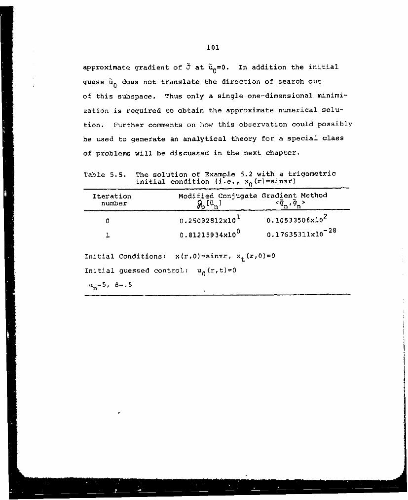
101

approximate gradient of J at %0=0. In addition the initial

guess u0 does not translate the direction of search out

of this subspace. Thus only a single one-dimensional minimi-

zation is required to obtain the approximate numerical solu-

tion. Further comments on how this observation could possibly

be used to generate an analytical theory for a special class

of problems will be discussed in the next chapter.

Table 5.5. The solution of Example 5.2 with a trigometricinitial condition (i.e., x 0 (r)=sin'lr)

Iteration Modified Conjugate Gradient Methodnumber ip [ 'In] gn' n>

0 0.25092812xi0 0.10533506xl0 2

1 0.81215934xi0 0 0.17635311xI0- 2 8

Initial Conditions: x(r,O)=sinrr, xt(r,O)=O

Initial guessed control: u 0 (r,t)=O

c± 5, =.5n

II

102

Table 5.6. The solution of Example 5.2 with a non-trigonometric initial condition (i.e., x0 (r)=r(l-r)0

Iteration Modified Conjugate Gradient Methodnumber ýp[5n] <gn 4n>

0 0.47825656x10-1 0.18528340xi0

1 0.18137734x10- 1 0.23826587x10- 2

2 0.18025130xl0- 0.11387571x0-5

3 0.18025621xi0-1 0.53594771xi0-6

4 0.18025653x0- 0.35357040xi0 9

5 0.18025653x10- 0.34480603x10 1 3

6 0.18025714x10- 0.74813105x10- 1 4

Initial Conditions: x(r,0)=r(l-r), xt(r,0)=0

Initial Guessed Control: u 0 (r,t)=0,

a n=5, 8=.5

Example 5.3.: The Boundary control of the vibrating string

The fixed time, penalized, minimum energy boundary control

of the vibrating string is considered. The problem may be

stated as follows:

minimize TF FJ[ub]=c I x 2 (rTf)dr + 6 J u(t)dt, (5.19)

0 1

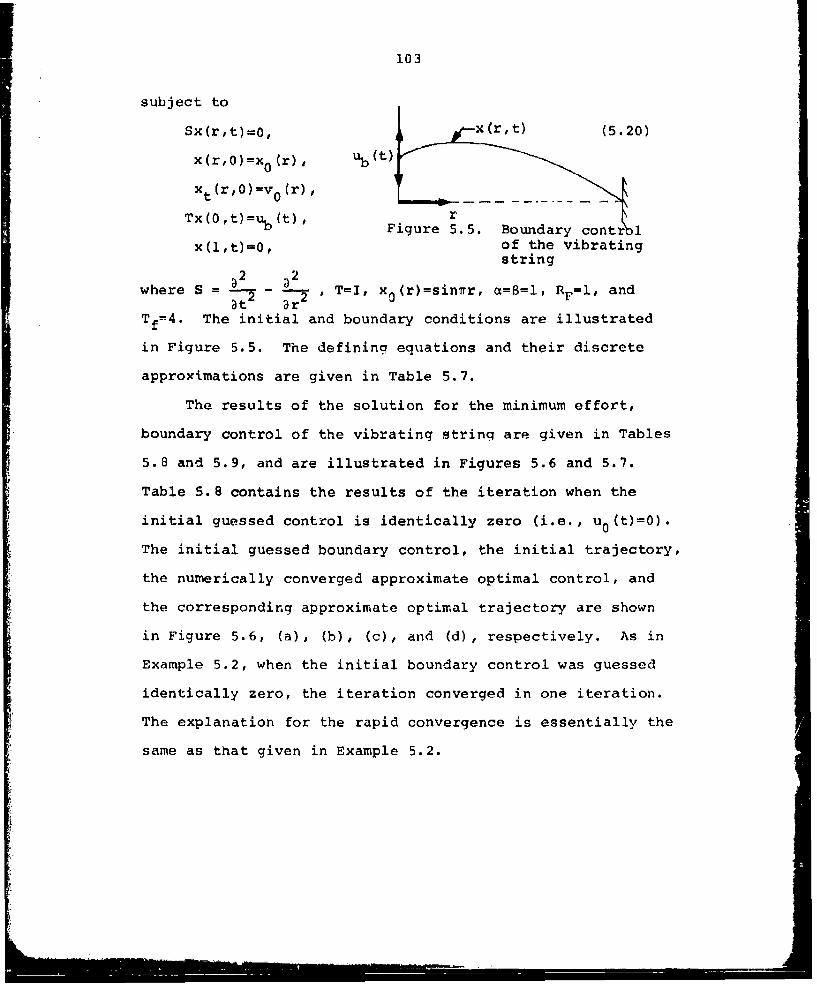
103

subject toSx(r,t)=0, i x(r,t) (5.20)

x(r,0)=x 0 (r) , Ub (t '

x t (r,0)--v0 (r), [- - - -trTx (0 , t) =0b(),

Tx(0't)=%(t)' Figure 5.5. Boundary contr 1

x(lt)=O0 of the vibratingstring

where S 2 r2 T=I, x 0 (r)=sinrr, a=6=l, RF=l, and

Tf--4 . The initial and boundary conditions are illustrated

in Figure 5.5. The defining equations and their discrete

approximations are given in Table 5.7.

The results of the solution for the minimum effort,

boundary control of the vibrating string are given in Tables

5.8 and 5.9, and are illustrated in Figures 5.6 and 5.7.

Table 5. 8 contains the results of the iteration when the

initial guessed control is identically zero (i.e., u 0 (t)=0).

The initial guessed boundary control, the initial trajectory,

the numerically converged approximate optimal control, and

the corresponding approximate optimal trajectory are shown

in Figure 5.6, (a), (b), (c), and (d), respectively. As in

Example 5.2, when the initial boundary control was guessed

identically zero, the iteration converged in one iteration.

The explanation for the rapid convergence is essentially the

same as that given in Example 5.2.

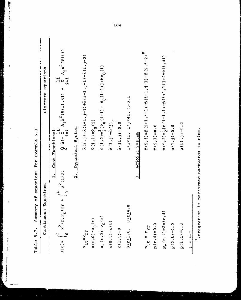
104

41 -'. ".411 --

'U H -4j 1 ~-

r- "-4 r- W+x ?-IH L,-4 4-'.4 1 1 1 11 1

E - - -om0 '- - - - r) ->, r-4 CNrl - - J n r4 N4En : - + -q V U+-

+- H 'r4 .j > - 4 ý -(N '.- '1'

(0 +x *'4 Ix . 0X *rx +4 ?o1. C

4J 00HH H V) X H( ~ Il IN 0 I

0 0U-[-~ 4) I I I II -. - i I i i4-- U d U . - r~ H G - . - - r .

0n 4 r - N '-b - H .. rJ N *- .0J-. ' C) - * - * H V )

E 1.

v 0 kWQ) -4 )

00

4'4 v-- 0)0 41 -4o ;i + .

-A- 0 JC- C0 '4Cd C14 c) .4 jNt

-4 0 H) - 4. I .CLn 4- 1-1 14 -- 0ý 114

'-4 4 - 04J -) 0 V 0- 0 4-14. (N 0> x 4. C)a 04

* X ii I 0 4.4 II 0 0

105

00

4J4

P4I

.-W

4J-

II*4

4 -I

nj L

4-I

u

It,

106

Table 5.8. Results for Example 5.3 with u 0 (t)=0Iteration

nutera n Modified Conjugate Gradient Methodnumber eUn -g'n

n ~[ýin gnrq

0 0.50185624xi00 0.88209975x1l

1 0.10027777xi0 0 0.31521281x10 2 8

ERROR ANALYSIS:

Optimal Control ERROR: ' *I < 0.17718170x10 0

Cost Functional ERROR: 1Jt, ,-9[u*]i < 0.20936213xl0

where le g(*,h) s- 0.35436341xi0f

J (a*;qh) 12 = 0.51743680xi0-1

and in = 0.28581078x10°

CPU time = 10.58 sec., Storage = 32400 BYTES.

aConverqence in one iteration occurred only when

u0 (t)=0 was used as the initial control quess.

The results of the iteration for a different initial

guess of the control (i.e., u0 (t)=-loe- tcos 2nt) are pre-

sented in Table 5.9. The initial guessed control, the

approximate optimal control, and the corresponding approxi-

mate optimal trajectory are illustrated in Figure 5.7, (a),

(b), and (c) respectively. The results contained in Table

5.8 and Figure 5.7 indicate that the modified conjugate

gradient method will converqe (as expected) from a relatively

poor initial guess. The converged solution from each of the

two different initial guesses are the same, as demonstrated

in Tables 5.8 and 5.9 and in Figures 5.6 and 5.7.

ir

107

Table 5.9. Results of Example 5.3 with uO (t)=-l0e- cos 27rt

Iteration The Modified Conjugate Gradient Methodnumber 9[a n]< ,n

0 0.26607469x10 2 0.22227374x10 3

1 0.13385153x102 O.10305737x103 0.17763568x101

2 0.83627214x10' I Q.14073426x10 3 -.0.57287508x101'1

3 0.24645929x10'1 0.38506615xl10 2 0.82156503x10 1 4

4 0.45224374x10 0 0.91346661x10 1 0.38941072x10-1 3

5 0.21074810x10 0 0.20603200x10'1 -0.19428902x10-1 5

6 0.J.4740533x10 0 0.33660356x10 0 0.21510571x10' 5

7 0.14688323x1O0 0.18495487x10 0 -0.13010426x10-1 6

8 0.10460883x1O0 O,34394526x10 0 0.18561541x10-1 5

9 0.96151817x10-1 O.61244688xl0'-1-0.49699827xl2- 1 5

10 0.97951980x10-1 0.19985723x101 0.10310762x10-1 5

11 0.10793993x1O0 0.52750740x10- 0.34640259xl10 1 6

12 0.l0831308x10 0 0.38984046x10- 0.22421300xJ-0 15

13 0.10187977xl10 0 0.43182735x101 0.11511516x10' 5

14 0.97608394xl 10 0.63656263xl10 -0.14007892x10-1 5

15 0.97377092xl 10 0.66l72248xl10 -0.81185058xl10 1 5

16 0.10327465x10 0 0.58561917x10- 0.13216424x10-1 5

17 0.10309298x10 0 0.470661.95x10- 2_0.37l00040iU0 1 7

18 0.10064508x10 0 0.25846288xl10 0.38916081xl10 1 6

19 0.10031671xl10 0 0.96233449x10-3 O.17208321xl10 1 6

20 0.10065392x1O0 0.37240919x10- 3_0.66204095xl101 6

21 0.10036221x10 0 0.1251.0802x10-4 _ 0.51698653xl101 7

CPU Time=34.5 sec (with three dimensional plot).

Storage =126 K (total).

108

.. 00 /

0.0in) THE GUESSED INITIAL CONTROL (wak, 1)- 0). b) THE INITIAL TRAJEC1ORY m0o, 0

.0.20 1 .0ý

0. 1.0

(A) THE APPROXIMATE OPT IMAAL IOUNDARY CONTROL (.) THE Of TIAL TRAJECTORY

Fiqure 5.6. The ,olution of the minimum onervcy houndarycorItrol of the vihratinq strina

109

u0@,t)

'$.0

(a) THE GUESSED INITIAL CONTROL (u 0(t) " - I co" oU 2,t).

hLb,

S0.20

4.0 ;?~

0.0

4. THE APPROXIMATE OiFt"AL BOUNDARY CONTROL

1'0

T) TH (TIMAL TRA.IECTORY

Figure 5.7. The solution of the minimum energy boundarycontrol of the vibrating strinq

The error analysis presented in Table 5.8 indicates

that the optimal control error and the cost functional error

are smaller than in Example 5.1. This is probably due to

the fact that there is less discretization in boundary control

problems than in distributed control problems. As indicated

in Tables 5.8 and 5.9 the storage, and the CPU times are

also reduced in this boundary control problem. The reduced

storage requirements are due to the fact that in boundary

control problems the control, the gradient, and the direction

of search are all singly subscripted arrays. The reduced

CPU times are due to the fact that in boundary control

problems there are no double integrals to be approximated.

The accuracy of the inner loop iterator is indicated

in column 4 of Table 5.9. The approximate directional

derivative at the one-dimensional minimum in the direction

n is given by <gn+lSn>, and theoretically should be zero.

However the numerical accuracy, which is in the order of

-1410-, is completely satisfactory. When the other inner

loop iterators were utilized <g ,S > was never smallern+l' n

than 10,-3 which demonstrates the validity of the conclusions

contained in Chapter IV.

z1

ill

CHAPTER VI. CONCLUDING REMARKS

The original objective of this investigation was to

develop practical means of optimizing distributed parameter

systems. The gradient methods appeared to be a promising

class of methods for solving distributed parameter optimal

control problems. However, early numerical results were

disappointing. Storage requirements and computation times

for test problems indicated that the study of complex dis-

tributed parameter systems would probably be beyond the stor-

age capabilities of the present computer system, and certain-

ly beyond a reasonable computer usage budget. Consequently,

as is the case in many investigations, the dissertation ob-

jectives were modified as work progressed. It soon became

apparent that in solving continuous distributed parameter

optimization problems on the digital computer the numerous

approximations involved in transforming the continuous problem

into a discrete problem were causing considerable errors. In

order to efficiently obtain an approximate solution, it be-

came evident that the understandinq of the effects of these

various approximations was essential. Therefore, the modified

objectives of developing an approximation theory for the

numerical optimization of distributed parameter systems were

considered. These objectives have been achieved for a

particular class of problems which are of practical signifi-

cance. Also, even though the original objective was not

112

achieved, substantial progress was made towards this objective.

An introduction to the optimization of distributed

parameter systems was presented in Chapter I, including a dis-

cussion of both the theoretical and the numerical results

which exist at the present time. Some of the engineering

applications for the optimization of distributed parameter

systems were also discussed.

A general theory for linear distributed parameter systems

was presented in Chapter II. The necessary conditions for a

local relative minimum were developed from the functional

* derivative point of view. It is felt that this development

is in the spirit of the subsequent use of gradient methods,

since it indicates exactly how the gradient of the cost func-

tional is to be calculated. The penalty function method was

introduced to render the constrained problems amenable to

gradient methods. A brief discussion of the various methods

of solving optimization problems was included.

The three most popular gradient methods were discussed in

Chapter III. A comparison between the conjugate gradient

method, the Davidon method, and the steepest descent method

was given. Three linear minimization methods were introduced,

a, discussed.

In Chapter IV the analysis of the effects of the many

approximations on the solution of the optimal distributed

parameter control problem was presented. It was found that in

113

the numerical optimization of distributed parameter systems

by gradient methods the round-off errors are negligible

when compared with other approximations involved. Further-

more, it became apparent that the approximations of

integral operators (e.g. , the cost functional, inner products,

etc.) could be made several orders of magnitude more accurate

than the approximations of the differential operators. Hence,

the two primary error sources were found to be, (1) the

approximation of functions, and (2) the approximation of dif-

ferential operators. It was also shown how these errors effect

the computation of the gradient vector, which obviously

directly influences the convergence of the approximate gradient

methods. In addition, it was demonstrated that the approxi-

mate gradient vector is the exact gradient of another quad-

ratic functional, defined on a subspace of the original control

space. This result, when coupled with the analysis of the

inner loop iteration, leads to necessary and sufficient con-

ditions for the numerical convergence of the approximate

gradient methods. It was shown that when method 3 (refer

to Theorem 4.2) is utilized in the inner loop then the approxi-

mate gradient methods converge to the minimum of J(.), not

J(-) nor its discrete analog •(.). This lead to the concept

of optimal control error and of the suboptimality of the

approximate solution. Results lading to the estimates of the

o ptimal control error and the suboptimality of the approximate

114

solution were established. A geometrical interpretation of

these estimates was included. It was recognized that these

estimates could be used to prove the convergence of the

approximate solution to the exact solution as discretization

tends to zero. Besides indicating the accuracy of a particular

solution, these error estimates yield a discernment into what

type of improvements to the approximate solution are feasible.

Numerical results for both the constrained and the un-

constrained optimal control of the one-dimensional wave

equation were given in Chapter V. Both distributed and

boundary control of the wave equation were considered. The

standard numerical comparisons between the modified conjugate

gradient method, the Davidon method, and the steepest descent

method were reported. It is evident from these results that

the second generation gradient methods offer a substantial

improvement over the steepest descent method, especially with

regard to the number of iterations required to achieve numeri-

cal convergence. This is particularly significant in the

minimization of distributed parameter systems, since each

iteration is very costly in terms of computer time. Although

the Davidon method converged faster (based on the number of

iterations), the modified conjugate gradient method required

considerably less storage and computer time to obtain com-

parable results. Thus, for the class of distributed parameter

systems considered the modified conjugate gradient method

115

appears to be the most efficient method of solution.

It was not expected that the Davidon method would con-

verge more rapidly than the conjugate gradient method, since

the theoretical results in (32) indicate that for this class

of problems these two iterations should produce the exact

same results. In (46) similar differences are reported for

the pure and the modified conjugate gradient methods on a

quadratic programming problem. The reasons given in (46)

for this behavior were based on round-off errors. However,

in this case the Davidon method is by far the more complex of

the two methods, and hence should be more sensitive to round-

off errors. It is doubtful that in general round-off errors

would increase the rate of convergence. Thus the answer to

this problem remains an open question.

Due to the discretization processes involved in the

solution of the optimization problem on a digital computer

the approximate gradient methods do not converged to the

exact solution. It was shown that this is due to gradient

error. Some authors have argued that when substantial gradient

errors are present the more powerful gradient methods should

not be used, since the effects of gradient errors might be

amplified by these methods. The results contained in this

work indicate that this is not necessarily the case. Cer-

tainly, it is true that in the presence of gradient errors

the gradient methods will not yield the exact solution.

116

However, if used properly, the more powerful gradient methods,

such as the conjugate gradient rrethod or the Davidon method,

find the approximate solution much faster; hence, at less

cost than the more simple gradient methods.

In conjunction with the theory and the numerical results

presented here, there remain many open problems. The ex-

tension of both the conjugate gradient method, and the

Davidon method to non-quadratic distributed parameter systems

is certainly feasible, and the potential results of such ex-

tensions appear to be very promising. An extension of the

error analysis presented in Chapter IV to nonlinear problems

would be of value. Also, consideration of a more conserva-

tive cost functional error estimate would be useful. Appli-

cations of numerical methods to bounded distributed parameter

control problems have not received a great deal of attention to

date. The results contained in Tables 5.5 and 5.7 indicate

that the application of a Ritz method to the class of problems

with trigonometric initial conditions may prove fruitful. In

addition, if the initial conditions are not trigonometric,

then they could be approximated by an appropriate Fourier

series, which could be conveniently truncated to obtain an

approximate solution. For problems with linear dynamics an

investigation of the penalty constants which circularize the

constant cost contours in the control space would be

beneficial, since this would increase the rate of convergence

117

for constrained problems. A more efficient method for pro-

gramming Davidon's method with emphasis placed on reducing

the storage requirements of the method would be a contribu-

tion. More sophisticated interpolation methods would most

likely reduce the optimal control error and the cost function-

al error. The utilization of cubic splines present interest-

ing possibilities. Finally, it is sugqested that the error

analysis and the approximation theory developed in this work

be applied to lumped parameter control problems, and to

parameter optimization problems (where the gradient vector

is obtained from a finite-difference formula).

Although much has already been accomplished, the interest

and the activity in this area still remains high; and it is

felt that this field still offers numerous possibilities

for research.

r

118

LITERATURE CITED

1. Butkovskii, A. G. and Lerner, A. Ya. The optimal controlof systems with distributed parameters. Automation andRemote Control 21: 472-477. 1960.

2. Butkovskii, A. G. Theory of optimal control fordistributed parameter systems. Moscow, Russia, Nayka.1965.

3. Lions, J. L. Contr6le optimal de syst'ms governispar des 4quations auix D~rivges Partielles. Paris,France, Dunod Gauthier-Villars. 1968.

4. Koppel, L. B. Introduction to control theory withapplications to process control. Englewood Cliffs,New Jersey, Prentice-Hall, Inc. 1968.

5. Denn, M. M. Optimization by variational methods.New York, New York, The McGraw-Hill Book Co. 1969.

6. Brogan, W. L. Optimal control theory applied to systemsdescribed by partial differential ecruations. Ph.D.dissertation. Los Angeles, California, UCLA. 1965.

7. Chaudhuri, A. K. Optimal control computational techniquesfor distributed parameter systems. Ph.D. dissertation.Gainesville, Florida, Florida University of Gaines-ville. 1967.

8. Dodd, C. W. An approximate method for optimal controlof distributed parameter systems. Ph.D. dissertation.Arizona State University. 1968.

9. Seinfeld, J. H. Optimal control of distributed-parametersystems. Ph.D. dissertation. Princeton, New Jersey,Princeton, University. 1967.

10. Wang, P. K. C. Optimal control of distributed-parametersystems. Transactions of ASME, Journal of Basic Engi-neering. Series D, 86: 67-79. 1964.

11. Wang, P, K. C. Theory of stability an6 control fordistributed parameter systems (a bibliography). Inter-national Journal of Control 7: 101-116. 1968.

12. Butkovskii, A. G., Egorov, A. I., and Lurie, H. A. Optimalcontrol of distributed systems (a survey of Soviet pub-lications). Society of Industrial Applied MathematicsJournal on Control 6: 437-476. 1968.

119

13. Robinson, A. C. A survey of optimal control of distrib-uted parameter systems. Aerospace Research Laboratoriesreport ARL 69-0177, prepared by the Battelle ColumbusLaboratories, Battelle Memorial Institute, Columbus,Ohio. 1969.

14. Butkovskii, A. G. The method of moments in the theoryof optimal control of systems with distributed parameters.Automation and Remote Control 24: 1106-1113. 1964.

15. Butkovskii, A. G. Optimum processes in systems withdistributed parameters. Automation and Remote Control22: 13-21. 1961.

16. Butkovskii, A. G. The maximum principle for optimumsystems with distributed parameters. Automation andRemote Control 22: 1156-1169. 1962.

17. Egorov, A. I. On optimum control of processes indistributed objects. Applied Mathematics and Mechanics(PMM) 27: 1045-1058. 1963.

18. Lurie, K. A. The Mayer-Bolza, problem for multiple inte-grals and the optimization of the performance of systemswith distributed parameters. Applied Mathematics andMechanics (PMM) 27: 1284-1299. 1963.

19. Balakrishnan, A. V. An operator theoretic formulationof a class of control problems and a steepest descentmethod of solution. Society of Industrial AppliedMathematics Journal on Control 1: 109-127. 1963.

20. Balakrishnan, A. V. Optimal control problems in Banach-spaces. Society of Industrial Applied MathematicsJournal on Control Series A, 3: 152-179. 1965.

21. Russell, D. L. Optimal regulation of linear symmetricalhyperbolic systems with finite dimensional controls.Society of Industrial Applied Mathematics Journal onControl 4: 276-294. 1966.

22. Axelband, E. I. Optimal control of linear distributedparameter systems. In Leondes, C. T., ed. Advances incontrol systems. Vol. 7. Pp. 257-310. New York, NewYork, Academic Press. 1969.

23. Weigand, W. A. and D'Souza, A. F. Optimal control oflinear distributed parameter systems with constrainedinputs. Transactions of ASME, Journal of Basic Enqineer-ing Series D 91: 161-167. 1969.

120

24. Sakawa, Y. Optimal control of a certain type of lineardistributed-parameter systems. IEEE Transactions forAutomatic Control AC-11: 35-41. 1966.

25. Magne, F. and Kristansen, T. Optimization of a non-linear distributed parameter system using periodicboundary control. International Journal of Control 10:601-624. 1969.

26. Lukes, D. L. and Russell, D. L. The quadratic criterionfor distributed systems. Society of Industrial AppliedMathematics Journal on Control 7: 101-102. 1969.

27. Phillipson, G. A. and Mitter, S. K. Numerical solutionof a distributed identification problem via a directmethod. In Balakrishnan, A. V. and Neustadt, L. W.,editors. Computing methods in optimization problems.New York, New York, Academic Press. 1969.

28. Sage, A. P. and Chaudhuri, S. P. Gradient and quasi-linearization computational techniques for distributedparameter systems. International Journal of Control 6:81-98. 1967.

29. Kim, M. M. Successive approximation method in optimumdistributed-parameter systems. Journal of OptimizationTheory and Applications 4: 40-43. 1969.

30. Denn, M. M. Optimal boundary control for a nonlineardistributed system. International Journal of Control 4:167-178. 1966.

31. Luenberger, D. G. Optimization by vector space methods.New York, New York, John Wiley and Sons, Inc. 1969.

32. Myers, G. E. Properties of the conjugate gradient andDavidon methods. Journal of Optimization Theory andApplications 2: 209-219. 1968.

33. Traub, J. F. Iterative methods for the solution ofequations. Englewood Cliffs, New Jersey, Prentice-Hall,Inc. 1964.

34. Kantorovich, L. V. On an effective method of solutionof extremal problems for a quadratic functional.Diklady Akademii Nauk SSSR 48: 483-487. 1945.

-' ..-. ...-

I121

35. Bryson, A. E., Jr. and Denham, W. F. Optimal programmingproblems with inequality constraints. II. solutionsby Steepest Descent. American Institute of Aeronauticsand Astronautics Journal 2: 25-34. 1964.

36. Bryson, A. E., Jr., Denham, W. F., and Dreyfus, S. E.Optimal programming problems with inequality constraints.I. Necessary Conditions for Extremal Solutions. AmericanInstitute of Aeronautics and Astronautics Journal 1:2544-2550. 1963.

37. Kelley, H. J. Gradient theory of optimal flight paths.American Rocket Society Journal 30: 947-954. 1960.

38. Hestenes, M. R. and Stiefel, E. Methods of conjugategradients for solving linear systems. Journal ofResearch of the National Bureau of Standards 49:409-436. 1952.

39. Hayes, R. M. Iterative methods of solving linear problemsin a Hilbert space. National Bureau of Standards AppliedMathematics Series 39: 71-104. 1954.

40. Daniel, J. W. The conjugate gradient method for linearand nonlinear operator equations. Society of IndustrialApplied Mathematics Journal on Numerical Analysis 4:10-26. 1967.

41. Antosiewicz, H. A. and Rheinbolt, W. C. Conjugate-direction methods and the method of steepest descentIn Todd, John, ed. Numerical analysis and functionalanalysis. Pp. 501-517. New York, New York,McGraw-Hill Book Co., Inc. 1962.

42. Fletcher, R. and Reeves, C. M. Function minimizationby conjugate gradients. The Computer Journal 7:149-154. 1964.

43. Lasden, L. S., Mitter, S., and Waren, A. D. The methodof conjugate gradients for optimal control problems.Institute of Electrical and Electronics Engineers Trans-action on Automatic Control AC-12: 132-138. 1967.

44. Sinnott, J. F., Jr. and Luenberger, D. G. Solution ofoptimal control problems by the method of conjugategradients. Joint Automatic Control ConferenceProceedings 1967: 566-574. 1967.

-- -- --

122

45. Daniel, J. W. Convergence of the conjugate gradientmethod with computationally convenient modifications.Numerische Mathematik 10:125-131. 1967.

46. Willoughby, J. K. Adaptations of the conjugate gradientmethod to optimal control problems with terminal stateconstraints. Ph.D. dissertation. Ames, Iowa, IowaState University. 1969.

47. Davidon, W. C. Variable metric method for minimization.Argonne National Laboratory Report ANL-5990 (Rev. 2)(Argonne National Lab., Argonne, 111.) Revised February1966.

48. Fletcher, R. and Powell, M. A rapidly convergentdescent method for minimization. The Computer Journal6: 163-168. 1963.

49. Horwitz, L. B. and Sarachik, P. E. Davidon's method inHilbert space. Society of Industrial Applied Mathe-matics Journal on Applied Mathematics 16: 676-695. 1968.

50. Tokumaru, H., Adachi, N., and Goto, K. Davidon'smethod for minimization problems in Hilbert space withapplications to control problems. Society of IndustrialApplied Mathematics Journal on Control 8: 163-178. 1970.

51. Pierson, B. L. and Rajtora, S. G. Computationexperience with the Davidon method applied to optimalcontrol problems. Engineering Research Institutepreprint 65000. Iowa State University, Ames, Iowa.1970.

52. Pierre, D. A. Optimization theory with applications.New York, New York, John Wiley and Sons, Inc. 1969.

53. Carnahan, B., Luther, H., and Wilkes, J. Appliednumerical methods. New York, New York, John Wiley andSons, Inc. 1969.

54. Kantorovich, L. V. and Akilov, G. P. Functional analysisin normed linear spaces. Translated from Russian byD. E. Brown, Edited by Dr. A. P. Robertson. New York,New York, The Macmillan Co. 1964.

55. Doerfler, T. E. The compounding of gradient error inthe method of parallel tangents, M.S. thesis. Ames,Iowa, Iowa State University. 1962.

, -- iii -.-. ii - ' i "-i i ' ii

123

5(. Stewart, G. W. A modification of Davidon's minimizationmethod to accept difference approximations of derivatives.Journal of the Association for Computing Machinery 14:72-83. 1967.

57. Cornick, D. E. and Seversike, L. K. Optimum parkingorbit orientation for a three-dimensional capture-escape mission. Journal of Spacecraft and Rockets 7:803-813. 1970.

58. Budak, B. M., Berkovich, E. M., and Solov'eva, E. N.Difference approximations in optimal control problems.Society of Industrial Applied Mathematics Journal on

Control 7: 18-31. 1969.

59. Cullum, J. Discrete approximations to continuousoptimal control problems 7: 32-49. 1969.

60. Richtmyer, R. D. and Morton, K. W. Difference methodsfor initial-value problems. 2nd Edition. New York,New York. Interscience Publishers. 1967.

61. Urabe, M. Convergence of numerical iteration in solu-tion of equations. Journal of Science of the HiroshimaUniversity Series A 19: 479-489. 1956.

62. Collatz, L. The numerical treatment of differentialequations. Berlin, Germany, Springer-Verlag. 1960.

63. Michel, A. N. System mathematics. Mimeographed classnotes, 595F. Ames, Iowa, Iowa State University,Department of Electrical Engineering. 1968.

64. Wilansky, A. Functional analysis. New York, New York.Blaisdell Publishing company. 1964.

65. Hildebrand, F. B. Methods of applied mathematics.2nd ed. Englewood Cliffs, New Jersey, Prentice-Hall,Inc. 1952.

66. Rivlin, T. J. An introduction to the approximation offunctions. Waltham, Massachusetts. Balisdell PublishingCompany. 1969.

67. Henrici, P. Discrete variable methods in ordinarydifferential equations. New York, New York, John Wileyand Sons, Inc. 1962.

I!

124

ACKNOWLEDGMENTS

The author wishes to thank Dr. A. N. Michel for his

enthusiastic guidance and suggestions concerning the research

reported in this dissertation. In addition, he wishes to

thank Dr. L. K. Seversike for his support and encouragement

throughout the author's undergraduate and graduate studies,

and to express his appreciation to his committee co-chairmen

Dr. E. W. Anderson and Dr. C. J. Triska for their assistance

during the degree program.

To his wife Mary no acknowledgment can possibly convey

the appreciation of her sacrifices and understanding over the

past years.

The author wishes to thank the Iowa State University

Research Foundation and the Office of Naval Research for

their financial support of this study, and Mrs. Gunnells for

her patience throughout the typing of the manuscript.

125

APPENDIX A. MATHEMATICAL PRELIMINARIES

In the development of an approximation theory for the

numerical optimization of distributed parameter systems,

results from several areas of applied mathematics are

utilized. The most important of these areas include (1)

numerical analysis, (2) functional analysis, (3) optimization

theory, (4) partial differential equations, and (5) approxi-

mation theory. In an attempt to make this dissertation

reasonably self-contained, a limited collection of definitions

and theorems from these areas will be presented. By necessity,

the treatment will be brief and incomplete; only material

which is used in this dissertation will be discussed. In

some instantancies standard definitions and results will be

altered to include concepts which are not introduced else-

where in this appendix. It will be assumed throughout, that

the reader is familiar with standard mathematical notation.

Selected Results from Functional Analysis

The natural setting for the application of gradient

methods to distributed parameter systems is a real separable

Hilbert space. The reasons for this are (1) gradient methods

require the concept of direction (hence, an inner product)

in the function space in which the iteration takes place, and

(2) separability and completeness are required in the proof

of convergence. Unfortunately, the definition of a Hilbert

v

126

space as "a complete inner product space" leaves much unsaid,

and consequently some additional preliminary concepts

need to be introduced.

Definition A-i: A linear space is a set X for which there

are defined an operation of addition denoted by +, so that

(X;+} is a commutative group; and an operation of scalair

multiplication satisfying the distributive law

a(x+y)=--x+6y,(a+B)x=ax+Bx, and (a8)x-c(ax), lx=x for all

x,yeX and a,$e Va scalar field.

In what follows the terms linear space and vector space

will be used interchangeably, and the elements of a linear

(vector) space will be referred to as vectors. If * is the

field of real numbers, then X is a real vectorr pace; if •*

is the field of complex numbers, then X is a complex vector

space.

Definition A-2; A nonempty subset S of a linear space X is

called a subspace in X if x+y is in S whenever x and y are

both in S and if also ax is in S whenever x is in S and a

is any scalar.

Definition A-3: A functional is a mapping of a linear space

1 1X into the scalars R , i.e., f: X+R

Definition A-4: An inner product on a linear space X is a

complex valued function of two elements selected from the

6L .

LI

127

space X, denoted by <x,y>, and satisfying the conditions:

Ui) <x,y> is linear as a function of x for fixed y.

(ii) <y,x> = <x,--> (the complex conjugate).

(iii) <x,x> >0 if xO.

Definition A-5: A norm is a real function, 1 I' , defined

on a linear space x satisfying, for all vectors x,yeX,

aE04the conditions:

(i) llxill > 0 xýo

(ii) Jl x+yll <_ lxi + I lyll (triangular inequality)

(iii) Ixl I = lal Jlxii (homogeneity).

Definition A-6: An inner product space is a linear space

together with an inner product defined on it.

Remark: In an inner product space the function

III = V 7.,.> is a norm.

Definition A-7: A Cauchy sequence in an inner product space

is a sequence {x n such that to each e>0, there corresponds

a number N such that I IXn-xmIMi < E whenever n>N and m>N.

Definition A-8: A normed linear space is said to be complete

if every Cauchy sequence in it is convergent (a normed linear

space is a linear space together with a norm).

The definition of a Hilbert space can now be given.

"II

128

Definition A-9: A Hilbert space is a complete inner product

space.

Definition A-10: A space is called separable if it contains

a countable dense subset.

In a separable Hilbert space there exists at least one

linearly independent set of vectors which spans the space.

Hence every vector can be written as a countable linear

combination of this linearly independent set. The partial

sums of this countable linear combinations forms a Cauchy

sequence; hence, conver:ge to a unique element in the space.

Another concept which is important is that of a linear

transformation.

Definition A-ll: If X and Y are linear spaces, a mapping

T: X-Y is a linear transformation, if for all scalars c,8,

T(ay+By)= cTx+$Ty, for all x,ycX.

Definition A-12: A linear operator is a linear transformation

of X into X, i.e., T:X-X.

Remark: The operator defined by

Lu = f f GF(rt;',T)u(ý,T)d•0 0

is linear (due to the properties of the definite integral).

Definition A-13: Let X and Y be n.'rmed spaces and let

129

AeB[X,YJ. The adjoint operator A*: Y*-X* is defined by the

equation <x,A*y*>=<Ax,y*>.

Definition A-14: An operator A defined on a Hilbert space

is said to be self-adjoint if A=A*.

Definition A-15: An operator A defined on a Hilbert space

is said to be a projection if A 2=A and A*=A, where A 2AA.

Definition A-16: A vector x is orthogonal to a subset M

of an inner product space X, if <x,y>=O for all ycM. This

is written xiM. The set of all such vectors is called the

annihilator of M and is written as K&. Thus

M = {x: xJ.M, xEX)

Theorem A-1: (63) (The Projection Theorem) If M is a sub-

space of X, then M+M =X, where X is a Hilbert space.

Definition A-17: It S be a subset of the domain of the

function f, where xEX, then an evaluation map E is defined

by E sf= {f(x); xCS}.

Definition A-18: A real valued functional f defined on a

convex subset C of a linear space is said to be convex if

f(�x 1 +(l- )x 2 ) < cf(xl)+(l- )f(x 2 )

for all xlx 2 C and all a, O<a<l.

L[2

130

Definition A-19: J[.] is a quadratic functional, defined on

a real Hilbert space X, if J[.] has the general form

Jfx]=J0+<c,X> + 1<xAx>,

where A is a linear operator.

Remark: It can be shown that a quadratic functional is

convex (52).

Theorem A-2: (22) (The existence of the Optimal Control)

If

(i) H is a Hilbert space (e.g., L2 ),

(ii) U is a closed convex bounded subset of H,

(Uii)J is a real continuous convex function on U,

then there exists a u*cU such that

J[u*] = inf J[u]

ucU

From Theorem A-2 the solution to the problem formulated

in Chapter II exists and is unique.

The following results are utilized by Chapter IV to

determine the spectral bounds of an operator.

Definition A-20: The set of all complex numbers X such that

A-XI is invertible (has an inverse) for a given operator A,

is called the resolvent set of A and is denoted by P(A).

131

Definition A-21: The spectrum of an operator A is denoted

by l(A), where a(A)={-X: Xfi(A)).

Lemma A-i: (64) Let AcB[H], where B[H] denotes the set

of bounded operators on H, a normed space, then A*A is self-

adjoint.

Lemma A-2: (64) If AcB[H], then I+A*A is self-adjoint.

Lemma A-3: (63) If A is self-adjoint, then a(A)CR1 .

Lemma A-4: (65) The spectrum of a skew symmetric operator

is pure imaginary (A is skew symmetric if A=-A*).

Lemma A-5: Let A be a completely continuous, skew symmetric

operator then

l<a'(I+A*A)

Another important theorem in analysis which is especially

useful in proving convergence of iteration formulas is the

Fixed Point Theorem. The basis of this theorem is the concept

of a contraction mapping.

Definition A-22: Let A be a mapping (not necessarily linear)

of a Hilbert space H (or Banach space or even a metric space)

into itself. Let for some o, O_<u<l,

I IA(x)-A(y)II < Ix-yI ,

for all y, ycH. Then A is said to be a contraction.

--------

132

Theorem A-3: (63) (Fixed Point Theorem) Every contraction

A, defined on a Hilbert space has one and only one fixed point,

i.e., Ax=x has one and only one solution for xcH. (This

theorem holds also for metric spaces).

In the optimal control of distributed parameter systems

the extension of the concept of a derivate in a Hilbert

space setting is useful.

Definition A-23: (31) Let XEDCX and let h be arbitrary

in X. If the limit

dJ = lir J[x+cth]-J [x]da C10 C1

exist, it is called the Gateaux differential of J at x with

increment h. If this limit exist for each heX, the functional

J is said to be Gateaux differentiable at x.

Definition A-24: (31) Let J be a transformation defined on an

open domain D in a normed space X and having range in a

normed space Y. If for fixed xcD and hcX there exists

6j(x;h)cY which is linear and continuous with respect to h

such that

lim HJ(x+h)-J(x)-SJ(x;h) . 0,

11h 11-0 Ilhil

then J is said to be Fre'het differentiable at x and

6J(x;h) is said to be the Fredhet differential of J at x

with increment h.

I

133

Pertinent Results from PartialDifferential Equations

The concept of well-posedness plays an important role in

the treatment of partial differential equations. It is

analogous to the concepts of exisLence and uniqueness of

solutions in ordinary differential equations. In this

dissertation an initial-value problem will be called well-

posed if

(i) a solution exist,

(ii) the solution is unique,

(iii) the solution depends continuously on the

initial data.

Reference (60) contains a detailed discussion of well-

posedness of the abstract Cauchy initial value problem.

Another important result used in Chapter II is the

representation of the solution of a partial differential

equation in terms of linear operators

-1x(r,t)=(t)X 0 + S-t)ud + T (t)ub (A-l)

Balakrishnan (20) has given conditions under which

Equation A-1 represents the solution to the nonhomogenous

partial differential equation. In this work only problems

for which the Green's function yields the representation given

in Equation A-1 are considered.

For example, consider the one-dimensional, non-homogenous

wave equation defined by

134

Xtt =Xrr + Ud? (A-2)

x(r,O)-O, (A-3)

xt(r,0)=0, (A-4)

x(0,t)=0, (A-5)

x(1,t)=0, (A-6)

This second order system can be rewritten as an equivalent

first order system by considering the transformation definedax ax

by v = and w = 7; hence, the above system becomes

at [w + (A-7)av a 0 vU d

at. r d.J

In order to obtain the Green's function for this problem,

the following eigenvalue problem is consideredF0

X k, (A-8)

2 2where ýk(o) -- (1)=0. The solution of this eigenvalue

problem yields Xk= + kri as the eigenvalues, and

2 [(A-9)0 2 (r) sin(kirr)

kI

135

as the eigenfunctions. By using these eigenfunctions, the

Green's function for this problem is given by

G F(r,t;&,T)=

E coskw(t-T)cosk~rr coskwFi E sink7r(t-T)cosk~rr sinkirk-l I k-I

2 (A-10)

- Z sinkv(t-T)sink~nr coskw 1l Z cosk•r(t-T)sinkrr sink~rýL k=1 tlk=l

which is represented byG 11 (r, t;&, T) GI12 (r' t; •'T)1j

GF(r,t;g,T)= (A-11)

LG2 (r,t;t, •) G2 (r,t;&,T)]

The solution of Equation A-7 can then be written as[wCr,t G1, G12 ]ft- f d~dT . (A-12)0 0

(r, t). G21 G1221 Ud ,T

From the above relation the Green's function for the original

problem can be determined as follows:

i I

136

x(r,t) = ra dr = w (r,t)dr (A-13)0 Dr0

= jrjtjl G1 2 Ud(&,T)d~dTdr

0 0 0G2udddd

= ftflfr G 12 U d drd~dtr

= o E 2sinkl(t-T)sink coskrrdrlud(&,T)d~dr,

by performing the above indicate integration, the Green's

function is determined as

G*(r t-,T)= E sink'n(t--r)sink•r& sinkerr. (A-14)F " * I k=l r

Numerical investigation of the convergence of this

series indicates that more than ten terms of this series

are required to obtain three significant digits of accuracy.

Pertinent Results from Approximation Theoryand Numerical Analysis

The fundamental problem of approximation theory may

loosely be stated as follows: determine R*c, where R is

a subspace of a linear space X, such that its distance from

x*eX is a minimum, that is, find x* such that I x*-xl I is

minimized. The following theorem is the basis of the approxi-

mation theory developed in Chapter IV.

137

Theorem A-4: (66) If X is a normed linear space and R is a

finite--dimensional subspace of X, then given x*cX, there

exists k*cR such that

IIx*-kx*II < llx*-xlI for all xek.

The following results are due to Kantorovich (54). Let

Sbe a complete subspace of the Hilbert space X, and let P

denote a projection from X onto R, i.e., PX=R, P 2=P, then

clearly P does not alter the elements of R. Consider two

iterations, the first in the space X

X n+lG(X n), (A-15)

and the second in the space R

(A-16)

In what follows Equation A-15 will be called the exact

iteration, and Equation A-16 the approximate iteration.

The spaces X and R, and the functions G and • will be

connected by the following conditions.

(i) (Condition that G and 6 be neighborinq functions)

for every kR,

PIG (A-17)

(ii) (Condition for elements of the form G(x) to be

approximated closely by elements of R.) For every

Xcx, there is an kcR such that

138

The above results are useful in answering problems en-

countered in this dissertation. These problems include:

(1) establishing the practicality and convergence of the

approximated gradient algorithms; (2) investigating the

speed of convergence; and, (3) obtaining suitable estimates

of the error.

In the analysis of the approximations due to dis-

cretizati.on, the approximate operator d often depends on a

parameter h, which is a measure of the discretization. By

extending the definition due to Henrici (67), the order of

an approximate operator can be defined as follows; if ý is

of order p then

?Cx;h) = c 4 P+l (p+l) (x+th) + 0(hp+2 )

where c is a constant, O<t<l, and lim O(h) 0

P+l h-O 11

This definition is standard in connecticn with the approxi-

mation of differential operators by difference operators, and

integral operators by summation operators.

The approximation of partial differential equations by

finite-difference operators results in errors. Before dis-

cussing these errors some additional nomenclature is

required.

139

Definition A-25: Let QxT denote the domain of a finite-

difference operator. Then the net (mesh, grid) which

partitions IxT is defined by

S= {(rt); r=ai and t = bi).

The nodes N of the net fl are the points of intersection

of the curves which define the net.(see Figure A-I).

-FUNCTION VALUE ONA NODE POINTGRAPH OF FUNCTION

NODE POINT

INET UNE

Figure A-1. The node N of the net

Definition A-26: Let x(ir,it) denote the exact solution of a

partial differential equation evaluated at the nodes of the

net. Then the truncation error (on the nodes) of the finite-

difference operator is defined as

et(ir, it) = x Ur, it) U (r, it) ,

where x is the approximate solution obtained from the finite-

difference method.

The second source of errors arises from the fact that

x cannot be calculated with exact precision because of the

limited accuracy of any computing equipment.

•, 14 0

Let k(ir,it) denote the values that are actually calculated

by the computer. The difference

r

is called the round-off error.

In addition to truncation errors, and round-off errors

there are interpolation errors. Interpolation errors are the

errors due to the approximation of functions (e.g., surfaces,

etc.) by interpolating functions. Let P denote the projection

from some class ef functions, which form a Hilbert space, to

the class of approximating functions. Then 11x-PxI! is a

IrLeasure of the accuracy of the interpolating functions.

L'

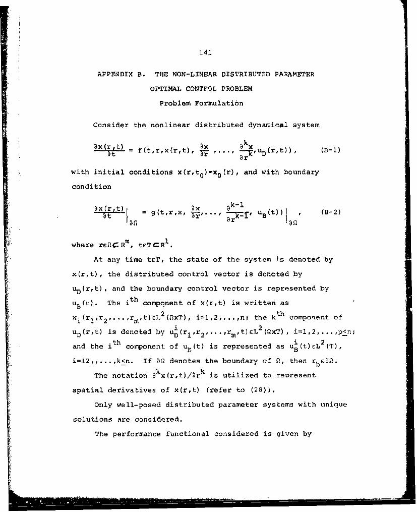
141

APPENDIX B. THE NON-LINEAR DISTRIBUTED PARAMETER

OPTIMAL CONTFOL PROBLEM

Problem Formulation

Consider the nonlinear distributed dynamical system

Dx(rt) = f(tjrvx(rjt), ;- , . -- (r,t)), (B-1)

with initial conditions x(r,t 0 )=X0 (r), and with boundary

condition

Dx(r,t) ax 9 k-iat " I = g(t,r,x, 3r,...r 9 _k-l u B(t)) Ia (B-2)

1where rcQCRm, teTCR

At any time teT, the state of the system is denoted by

x(rt), the distributed control vector is denoted by

uD(r,t), and the boundary control vector is represented by

uB(t). The ith component of x(r,t) is written as

xi(rir 2 ,...,rmt)EL2(nxT), i=l,2,...,n; the kth component of

uD(rt) is denoted by uD ,t 2 (xT), i=l,2,...,p.n;

and the ith component of u (t) is represented as u i(t)£L2(T),

i=I2,,...,k<n. If an denotes the boundary of Q, then rbED.

The notation akx(rt)/Drk is utilized to represent

spatial derivatives of x(r,t) (refer to (28)).

Only well-posed distributed parameter systems with unique

solutions are considered.

The performance functional considered is given by

It 142

J[uD(r,t),uB(t)) Glx,r,Tf) 1+ T[Kx(r,Tf)]da

a x akx

+ L, ... , --- , dt (B-3)" T Br ;r

+ I a x akx UDddt+ f 7 LD(t,r,x, 3 *, U..)dS dt,ST J r

where

Sfr 1I r2 rm

and LD, K, and G are sufficiently smooth real valued functions.

The optimum control problem is now stated as follows:

determine from the set U of admissible controls the control

vector u,

uT = [uD, UB], uEU, (B-4)

which satisfies the state equations along with the initial

and the boundary conditions and at the same time minimizes

Jf[uD uB •(1D' B1

Derivation of the NecessaryConditions

Let J be the functional defined by Equation B-3. In

order for J to have a relative local minimum at u*cU, it is

necessary that the first Fre6het derivative of J at u* be

identically zero, that is

143

IJ = lir J[u]-J[u*J = 0 . (B- 5)S~u* u-u* l lu-u*i i

Let p(r,t) denote the Lagrange multiplier associated

with the dynamical system, and let X(t) denote the Lagrange

multiplier associated with the boundary conditions. By using

the Lagrange multipliers p(r,t) and X(t), the constrained

problem defined by Equations B-i, B-2, and B-3 can be re-

formulated as an unconstrained problem, where the unconstrained

cost functional is given by

JLuT=G + {LB + <,\g- ytI> )dt + JK dl (B-6)

+ f - >dQ dt.tTJf D

If the constraints are satisfied then mn rin J . Thus,

the minimum of J can be obtained from the minimum of •. In

the following development it will be assumed that the con-

straints are satisfied and hence, 3=J.

Let HD denote the distributed Hamiltonian, and let H

denote the boundary Hamiltonian, where

HD = LD + <p,f>, (B-7)

and

HB = 1B + <X'g>. (B-8)

1 The arguments of G, LB, A, g, f, X, LD, p, and xwill be dropped for notational simplicity.

144

Substitution of the distributed and the boundary Hamil-

tonians into Equation B-6 yields

J[u]=G+ K dcQ + f[HB-<X, 'x- >]dtQ fT B t n

[ I [ PA, ax>]dQ dt . (B-9)

From Equation B-8 the difference J[u]-J[u*J is given by

J(u]-J[u*]=G-G*+f (K-K*)dn

+ H -H*-<Xl a -- * >]dt+ TB B a t; at a

+ [H -HI -<,-@ ] d dt. (B-10)

f~nD D at

Now perturb the control u* by letting u=u*+cw, and

let x=x*+EY denote the trajectory corresponding to u.

Expanding the terms in Equation B-9 about u* and x* in a

Taylor's series yields

G-G-= . Tf + ... + 0(c), (B-11)

K-K*=E<-K IT> + " + 0(c), (B-12)ax* Tf

145

aHB k-i DHDH

H H*C T B BHB-H B a•x- Ia 5 i x r au

+ 0(c) (B-13)

aHD k aHD k a Y HD-H <---I• ,T>+Eil<-ri•, --- >+c -' >+0 (),

D D a UD

(B-14)

and

ax ax* = (B-15)at at -at

where

T= T T T[n Is ], and 1rn 0 0.

Substitution of Equations B-il, B-12, B-13, B-14, and

B-15 into B-10, and integrating by parts yields

lrn J1u1-J3u*] < 2G I I +T <n a Kli0 E X,> + - -P Y>I dQ

:- ax IaITf ax IT•Tf n f

(B-16)

+ k- i ai 9H D +- I a H~ ~ >I+j~ ~ ~ ~a ; -)•1• ~- I x k k-l •a

Ti=0 7r ri+l r

k-1 k=iJ- HD _HB

+ E < (-1)3 -r 1+ T >1 Idti=2 j=0 ar r< - •r i_' r r ,

31H k i 3HD+< -- + (-) --- + . T,'>+<= ,n>) dt.

JTJ X i=l r i br

146

Optimality Conditions

It follows from Equation B-15 that in order for

[u0T, u*T to be optimal, it is necessary that there exist

functions p*(r,t) and X*(t) such that

a. x*(r,t) is a solution of the distributed state system

w= f, x(rt 0 ) = x 0 (r)' g 1 " (B-17)

b. p*(r,t) is a solution of the distributed costate

system

Lp 3H D k i iaH D+ -- -k " + ; r 1-p ( r T f ) =

-- (r•x~r t) "(13-18)

t=f

c. X*(t) is a solution of the ordinary differential

equation

d • + P(-) B- k-1 T a (B-19)i=O irx i

X(T f)= i t=TfMllt=T

147

d. The transversality conditions are satisfied, i.e.,

MD k k-i aj DHD -

0 ax i-1 JK0 + axri+J Ian(B-20)

i=2 ,3, • . • ,k-l.

e. The gradient of J vanishes, i.e.,

Tm T T Tg (u)'r [go (u)' 9B (u)T]- [ (a)H/a uD)r (B-21)

(MHB/auB)T [0T0 T 1 T

Im. . ..! .