THE NUMERICAL COMPUTATION OF VIOLENT WAVES APPLICATION · PDF fileTHE NUMERICAL COMPUTATION OF...

THE NUMERICAL COMPUTATION OF VIOLENT WAVES –

APPLICATION TO WAVE ENERGY CONVERTERS

Frédéric DIAS School of Mathematical Sciences

University College Dublin

on leave from Ecole Normale Supérieure de Cachan

26 July 2011 – WAVES 2011 - Vancouver

26 July 2011 - Vancouver1

Oyster Aquamarine Power 2009

TOPICS COVERED IN TODAY’S TALK

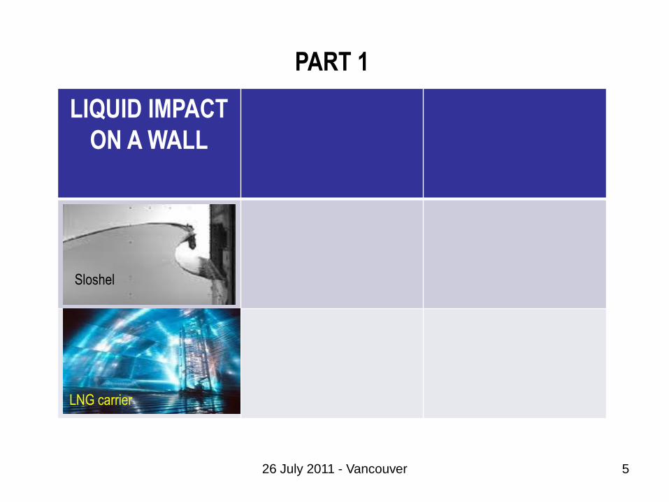
LIQUID IMPACT

ON A WALL

TSUNAMIS FREAK WAVES

Thailand 2004 South Carolina 1986

Spain 2010

Japan 2011

226 July 2011 - Vancouver

Sloshel

LNG carrier

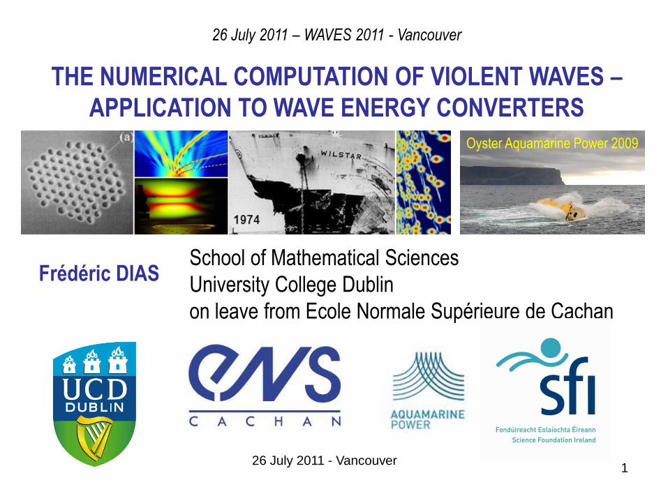
Aquamarine Power is a technology company that has

developed a product called Oyster which produces

electricity from ocean wave energy.

UCD and Aquamarine Power are

collaborating to deliver the next-

generation Oyster 800.


WAVE ENERGY CONVERSION


Jean-Philippe Braeunig (INRIA & CEA)

Laurent Brosset (GTT)

Paul Christodoulides (Cyprus University of Technology)

Ken Doherty (Aquamarine Power Ltd.)

John Dudley (University of Franche-Comté)

Denys Dutykh (University of Savoie)

Christophe Fochesato (CEA)

Jean-Michel Ghidaglia (Ecole Normale Supérieure de Cachan)

Laura O‟Brien (University College Dublin)

Raphaël Poncet (CEA)

Themistoklis Stefanakis (University College Dublin & ENS-Cachan)

Research funded by

FP6 EU project TRANSFER (Tsunami Risk ANd Strategies For the European Region)

ANR (French Science Foundation)

SFI (Science Foundation Ireland)

GTT (Gaz Technigaz & Transport)

COLLABORATORS

PART 1

LIQUID IMPACT

ON A WALL


Sloshel

LNG carrier

WAVE IMPACT AND PRESSURE LOADS

6

•Local phenomena involved during wave impacts are very sensitive to input conditions

•The density of bubbles, the local shape of the free surface, the local flow make the

impact pressure change dramatically even for the same experimental conditions

•How does one extrapolate wave impact from model (small scale) to prototype (full

scale)?

•In recent years, we have addressed the scaling issue by studying the various local

phenomena present in wave impact one after the other in order

to better understand the physics behind

to improve the experimental modelling

VIDEO 1 – Experiments in Marseille

(courtesy of O. Kimmoun)

Source : Peregrine D.H. (2003), Water wave impact on walls, Annual Review of Fluid Mechanics


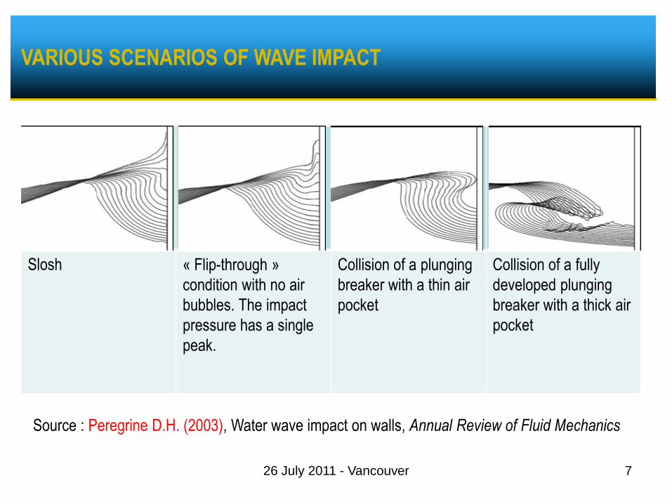
VARIOUS SCENARIOS OF WAVE IMPACT

Slosh « Flip-through »

condition with no air

bubbles. The impact

pressure has a single

peak.

Collision of a plunging

breaker with a thin air

pocket

Collision of a fully

developed plunging

breaker with a thick air

pocket

Bredmose et al. (2004), Water wave

impact on walls and the role of air,

Proceedings ICCE 2004

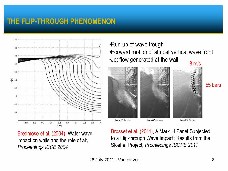
•Run-up of wave trough

•Forward motion of almost vertical wave front

•Jet flow generated at the wall


THE FLIP-THROUGH PHENOMENON

Brosset et al. (2011), A Mark III Panel Subjected

to a Flip-through Wave Impact: Results from the

Sloshel Project, Proceedings ISOPE 2011

8 m/s

55 bars

Global behaviour

Global flow governed by Froude number

Local behaviour

Escape of the gas between the liquid and the wall:

momentum transfer between liquid and gas

Compression of the partially entrapped gas during the last

stage of the impact

Rapid change of momentum of the liquid diverted by the

obstacle

Possible creation of shock waves: pressure wave within the

liquid and strain wave within the wall

Hydro-elasticity effects during the fluid-structure interaction

PHENOMENOLOGY OF A LIQUID IMPACT


Braeunig et al. (2009), Phenomenological Study of Liquid Impacts through 2D Compressible

Two-fluid Numerical Simulations, Proceedings ISOPE 2009

10

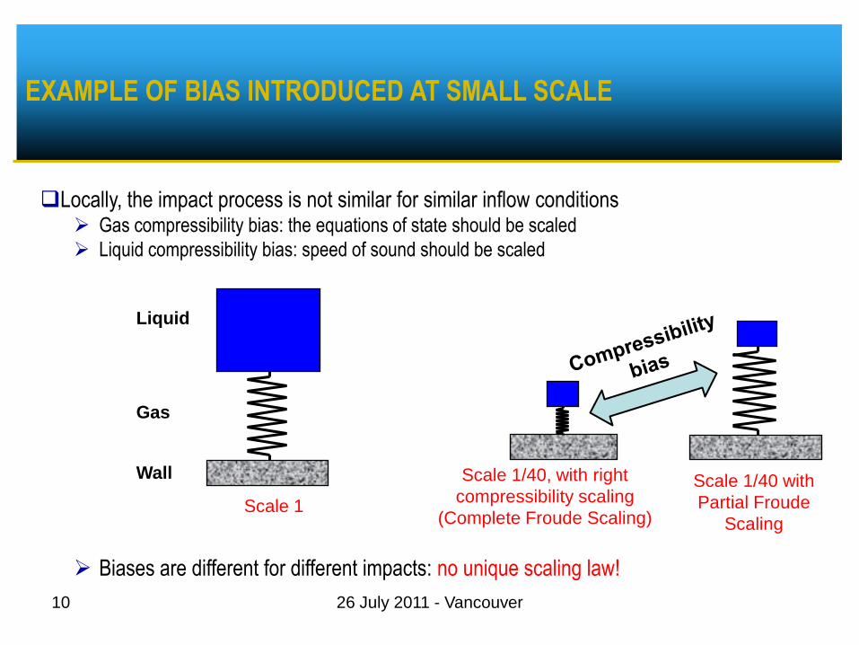
Locally, the impact process is not similar for similar inflow conditions Gas compressibility bias: the equations of state should be scaled

Liquid compressibility bias: speed of sound should be scaled

Biases are different for different impacts: no unique scaling law!

Liquid

Gas

Wall

Scale 1

Scale 1/40, with right

compressibility scaling

(Complete Froude Scaling)

Scale 1/40 with

Partial Froude

Scaling

EXAMPLE OF BIAS INTRODUCED AT SMALL SCALE



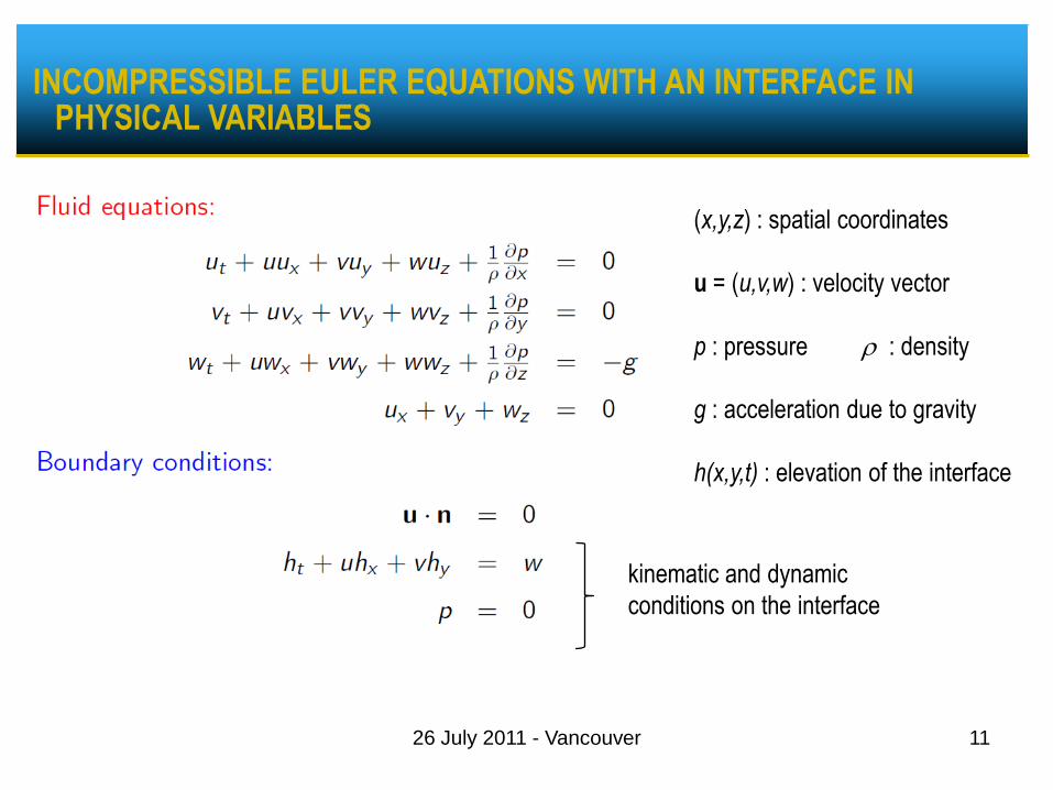
INCOMPRESSIBLE EULER EQUATIONS WITH AN INTERFACE IN PHYSICAL VARIABLES

(x,y,z) : spatial coordinates

u = (u,v,w) : velocity vector

p : pressure r : density

g : acceleration due to gravity

h(x,y,t) : elevation of the interface

kinematic and dynamic

conditions on the interface


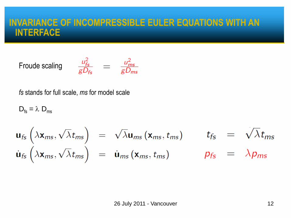
INVARIANCE OF INCOMPRESSIBLE EULER EQUATIONS WITH AN INTERFACE

Froude scaling

fs stands for full scale, ms for model scale

Dfs = l Dms


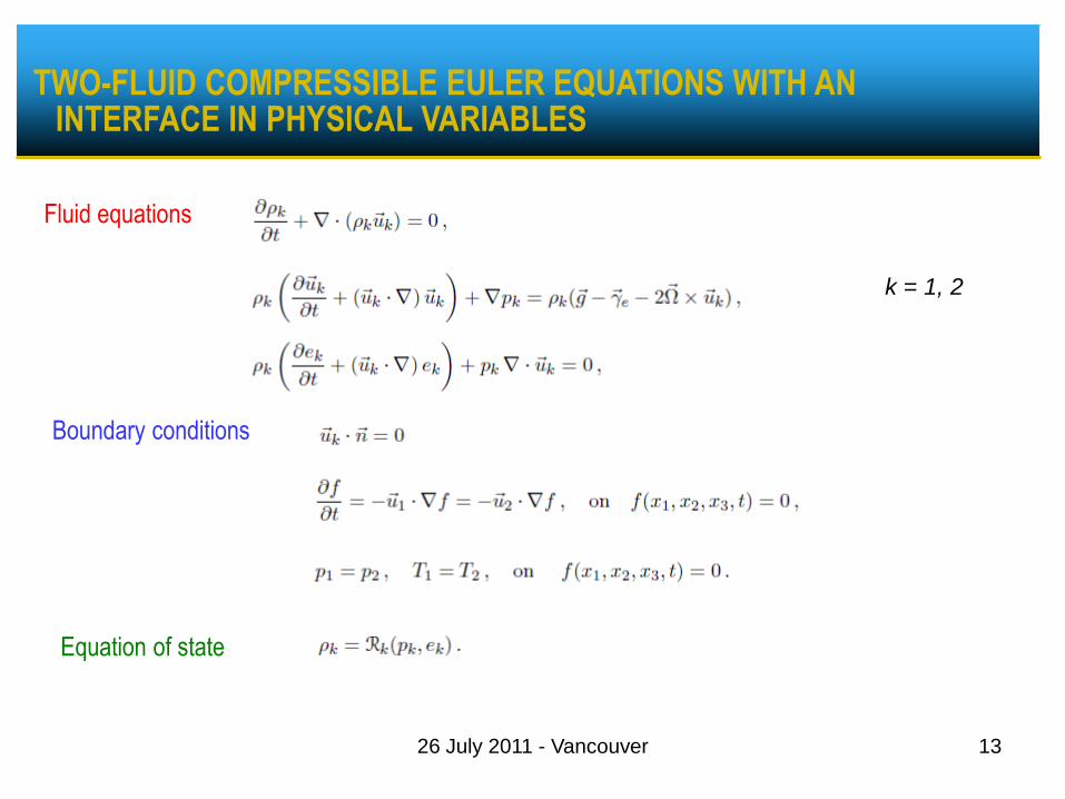
TWO-FLUID COMPRESSIBLE EULER EQUATIONS WITH AN INTERFACE IN PHYSICAL VARIABLES

Fluid equations

Boundary conditions

k = 1, 2

Equation of state


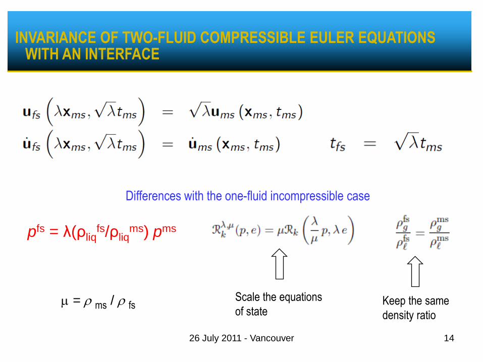
INVARIANCE OF TWO-FLUID COMPRESSIBLE EULER EQUATIONS WITH AN INTERFACE

pfs = λ(ρliqfs/ρliq

ms) pms

Differences with the one-fluid incompressible case

Scale the equations

of stateKeep the same

density ratio

m = r ms / r fs

THE ROLE OF NUMERICAL STUDIES

15

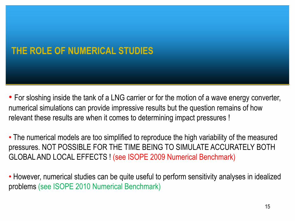
• For sloshing inside the tank of a LNG carrier or for the motion of a wave energy converter,

numerical simulations can provide impressive results but the question remains of how

relevant these results are when it comes to determining impact pressures !

• The numerical models are too simplified to reproduce the high variability of the measured

pressures. NOT POSSIBLE FOR THE TIME BEING TO SIMULATE ACCURATELY BOTH

GLOBAL AND LOCAL EFFECTS ! (see ISOPE 2009 Numerical Benchmark)

• However, numerical studies can be quite useful to perform sensitivity analyses in idealized

problems (see ISOPE 2010 Numerical Benchmark)

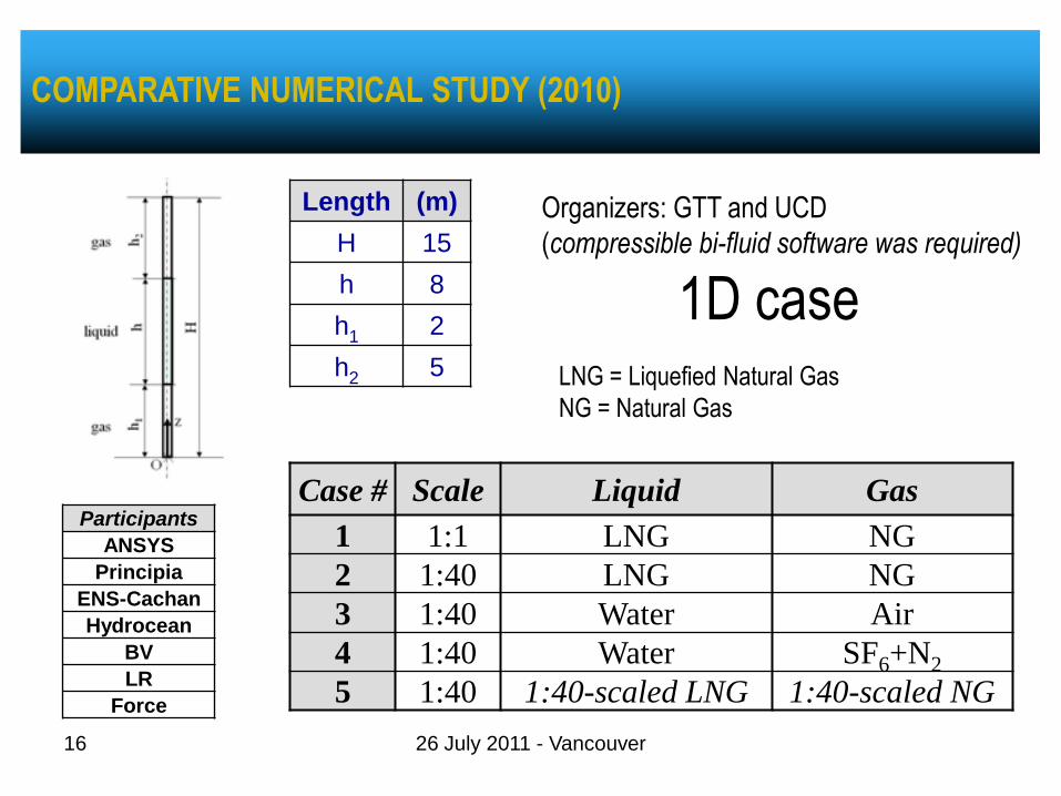
1D case

16

Length (m)

H 15

h 8

h1 2

h2 5

Case # Scale Liquid Gas

1 1:1 LNG NG

2 1:40 LNG NG

3 1:40 Water Air

4 1:40 Water SF6+N2

5 1:40 1:40-scaled LNG 1:40-scaled NG

Participants

ANSYS

Principia

ENS-Cachan

Hydrocean

BV

LR

Force

COMPARATIVE NUMERICAL STUDY (2010)

Organizers: GTT and UCD

(compressible bi-fluid software was required)

LNG = Liquefied Natural Gas

NG = Natural Gas


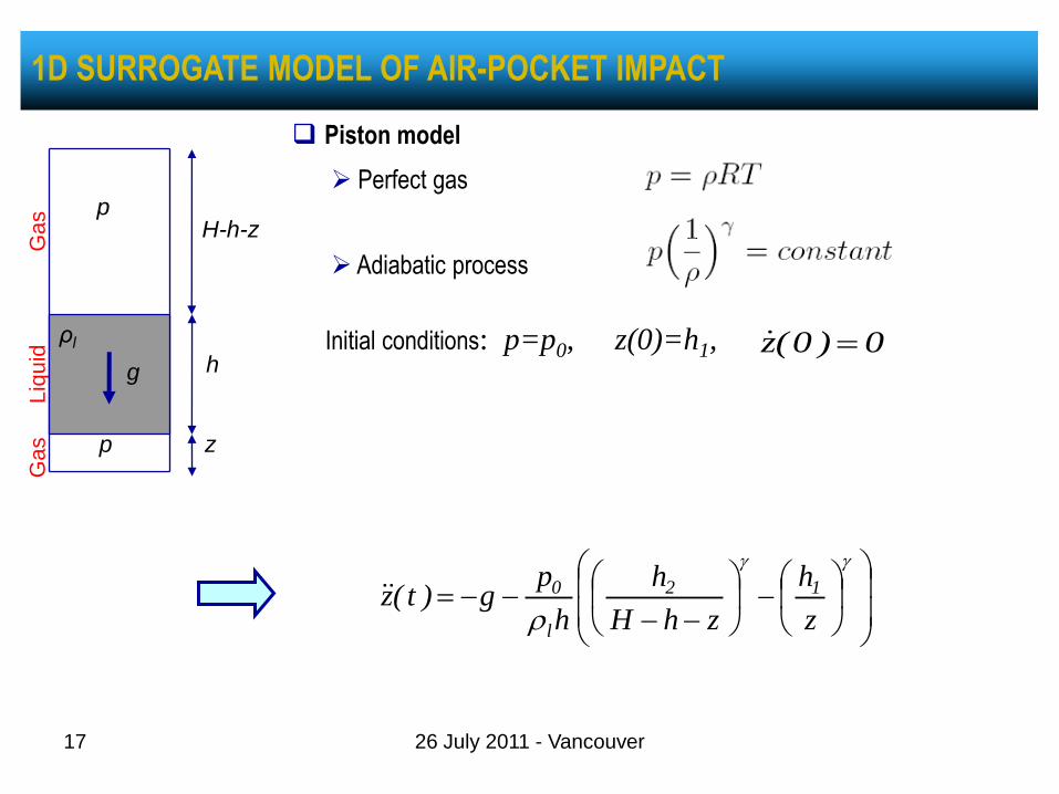
Piston model

Perfect gas

Adiabatic process

17

Liq

uid

Gas p

p

Ga

s

g

ρl

z

h

H-h-z

r z

h

zhH

h

h

pg)t(z 12

l

0

Initial conditions: p=p0, z(0)=h1, 0)0(z

1D SURROGATE MODEL OF AIR-POCKET IMPACT


0.0E+00

1.0E+04

2.0E+04

3.0E+04

4.0E+04

5.0E+04

6.0E+04

7.0E+04

0.0 0.1 0.2 0.3 0.4 0.5 0.6 0.7 0.8 0.9 1.0 1.1 1.2

Pre

ssu

re (P

a)

Time (s)

Pressures at full scale: theoretical model

Case 1

Case 2

Case 3

Case 4

18

Case 5 = Case 1Warning:

Compressibility matters,

when comparing at same scale

The 5 cases are very

smooth compression cases

Pressures and times are Froude-scaled for cases 2, 3, 4, 5 pfs = λ.(ρliqfs/ρliq

ms).pms tfs = √λ.tms

with λ = 40, fs = full scale, ms = model scale

THEORY : PRESSURES IN TIME DOMAIN


The different numerical methods are able to simulate adequately a

simple smooth compression of a gas pocket without escape of gas

Very good agreement on the maximum pressure

For all methods :

Complete Froude Scaling (CFS) works (same result for cases 1

& 5)

Partial Froude Scaling (PFS) generates a bias

CONCLUSIONS FOR THE 1D CASE


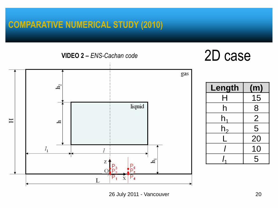
2D case

Length (m)

H 15

h 8

h1 2

h2 5

L 20

l 10

l1 5

COMPARATIVE NUMERICAL STUDY (2010)


VIDEO 2 – ENS-Cachan code

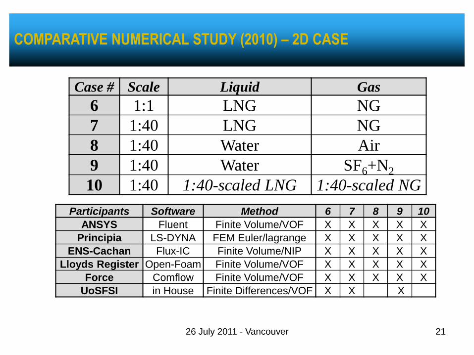
Case # Scale Liquid Gas

6 1:1 LNG NG

7 1:40 LNG NG

8 1:40 Water Air

9 1:40 Water SF6+N2

10 1:40 1:40-scaled LNG 1:40-scaled NG

Participants Software Method 6 7 8 9 10

ANSYS Fluent Finite Volume/VOF X X X X X

Principia LS-DYNA FEM Euler/lagrange X X X X X

ENS-Cachan Flux-IC Finite Volume/NIP X X X X X

Lloyds Register Open-Foam Finite Volume/VOF X X X X X

Force Comflow Finite Volume/VOF X X X X X

UoSFSI in House Finite Differences/VOF X X X

COMPARATIVE NUMERICAL STUDY (2010) – 2D CASE


-1.0E+05

0.0E+00

1.0E+05

2.0E+05

3.0E+05

4.0E+05

5.0E+05

6.0E+05

0.5 0.6 0.7 0.8 0.9 1

Pre

ssu

re (P

a)

Time (s)

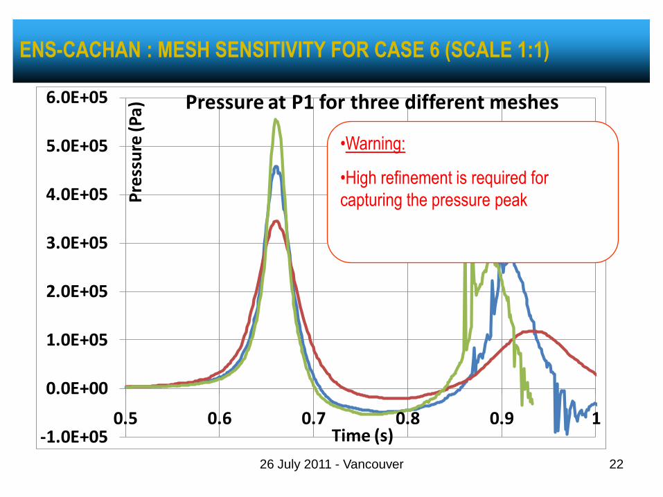
Pressure at P1 for three different meshes

P-P0 cas6 dx=0.05m

P-P0 cas6 dx=0.1m

P-P0 cas6 dx=0.0333m

•Warning:

•High refinement is required for

capturing the pressure peak

ENS-CACHAN : MESH SENSITIVITY FOR CASE 6 (SCALE 1:1)


Velocities and times are Froude-scaled for cases 7, 8, 9, 10

Vfs = √λ.Vms , tfs = √λ.tms with λ = 40, fs = full scale, ms = model scale

horizontal velocity in P5 at full scale: ANSYS

-15

-5

5

15

25

35

45

55

65

75

85

0 0.1 0.2 0.3 0.4 0.5 0.6 0.7 0.8 0.9 1Time (s)

Vx

(m/s

)

Case 6

Case 7

Case 8

Case 9

Horizontal velocity in P5 at full scale: PRINCIPIA

0

10

20

30

40

50

60

70

80

90

100

110

120

130

0 0.1 0.2 0.3 0.4 0.5 0.6 0.7Time (s)

Ve

loci

ty (

m/s

)

Case 6Case 7Case 8Case 9Case 10

Horizontal velocity in P5 at full scale: ENS-Cachan

0

10

20

30

40

50

60

70

80

90

100

110

120

130

140

0 0.1 0.2 0.3 0.4 0.5 0.6 0.7Time (s)

Ve

loci

ty (

m/s

)


Horizontal velocity in P5 at full scale: Lloyds Register

0

5

10

15

20

25

30

35

40

45

50

55

0 0.1 0.2 0.3 0.4 0.5 0.6 0.7Time (s)

Ve

loci

ty (

m/s

)


Horizontal velocity in P5 at full scale: Force Technology

0

2

4

6

8

10

12

14

16

18

20

22

24

26

0 0.1 0.2 0.3 0.4 0.5 0.6 0.7Time (s)

Ve

loci

ty (

m/s

)


Horizontal velocity in P5 at full scale: U. of Southampton

-10

-5

0

5

10

15

20

25

30

35

40

0 0.1 0.2 0.3 0.4 0.5 0.6 0.7

Time (s)

Ve

loci

ty (

m/s

)

Case 6

Case 7

Case 8

Case 9

Case 10

HORIZONTAL TIME SERIES AT P5 : ALL PARTICIPANTS


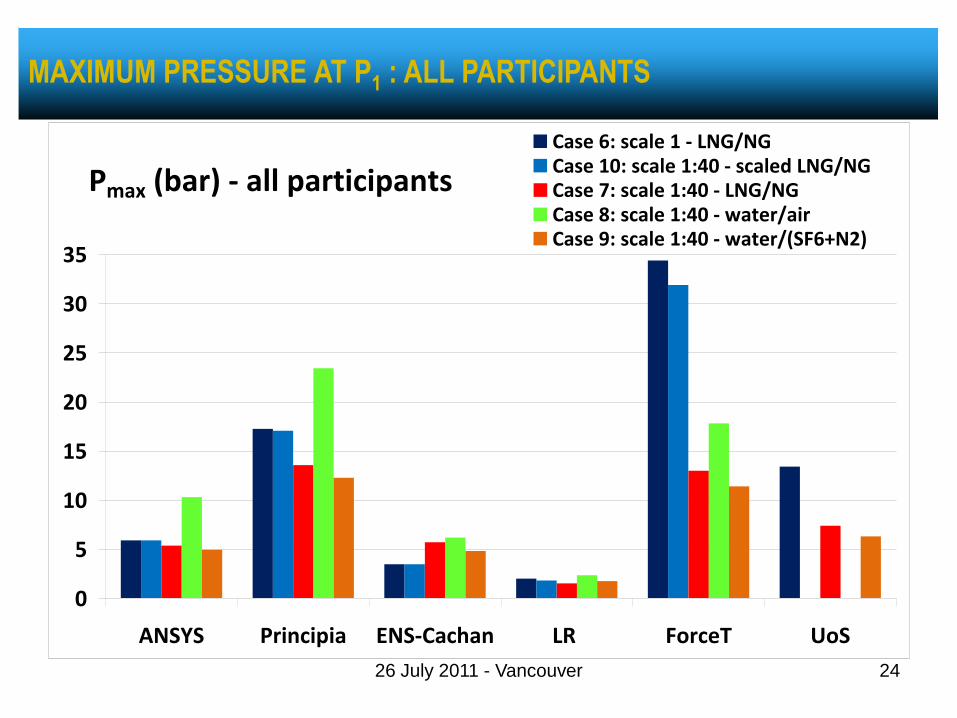
Pmax (bar) - all participants

0

5

10

15

20

25

30

35

ANSYS Principia ENS-Cachan LR ForceT UoS

Case 6: scale 1 - LNG/NGCase 10: scale 1:40 - scaled LNG/NGCase 7: scale 1:40 - LNG/NGCase 8: scale 1:40 - water/airCase 9: scale 1:40 - water/(SF6+N2)

MAXIMUM PRESSURE AT P1 : ALL PARTICIPANTS


Absolute values for Vmax and Pmax are very scattered

The meshes are not refined enough to capture sharp peak pressures

After some work on the models, results should be much less scattered

(work in progress)

Such a simple test should be passed adequately before

attempting to calculate more complex impacts

For all methods, whether relevant or not :

Complete Froude Scaling (CFS) is satisfied

Partial Froude Scaling generates a bias

COMPARATIVE NUMERICAL STUDY (2010) – 2D CASE


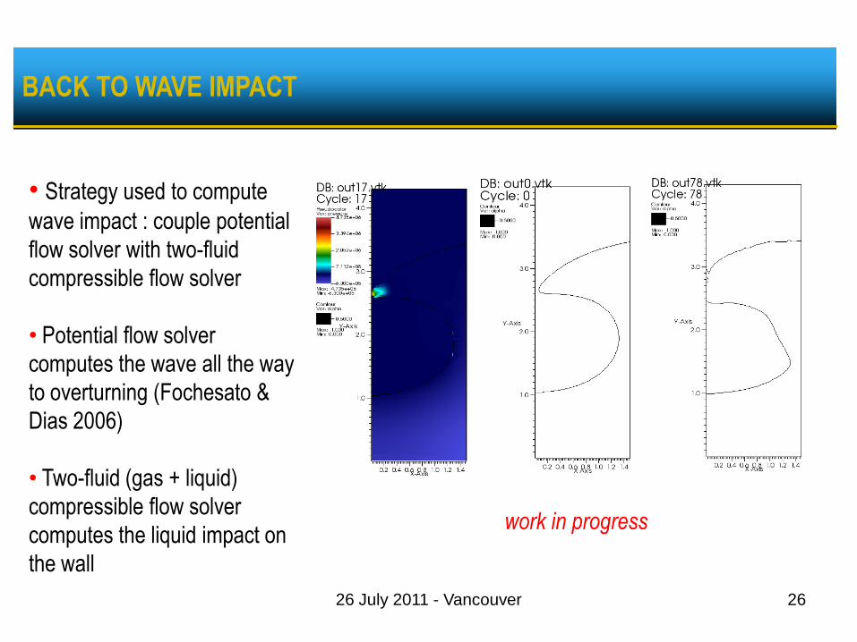
BACK TO WAVE IMPACT


• Strategy used to compute

wave impact : couple potential

flow solver with two-fluid

compressible flow solver

• Potential flow solver

computes the wave all the way

to overturning (Fochesato &

Dias 2006)

• Two-fluid (gas + liquid)

compressible flow solver

computes the liquid impact on

the wall

work in progress

PART 2

TSUNAMIS

Thailand 2004

Japan 2011


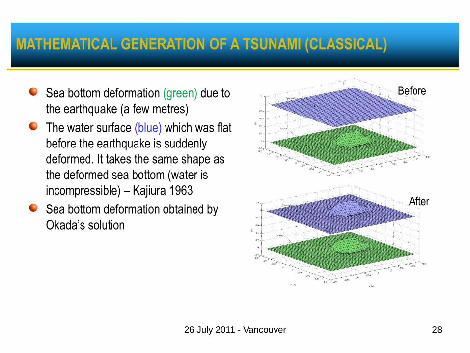
Sea bottom deformation (green) due to

the earthquake (a few metres)

The water surface (blue) which was flat

before the earthquake is suddenly

deformed. It takes the same shape as

the deformed sea bottom (water is

incompressible) – Kajiura 1963

Sea bottom deformation obtained by

Okada‟s solution

Before

After


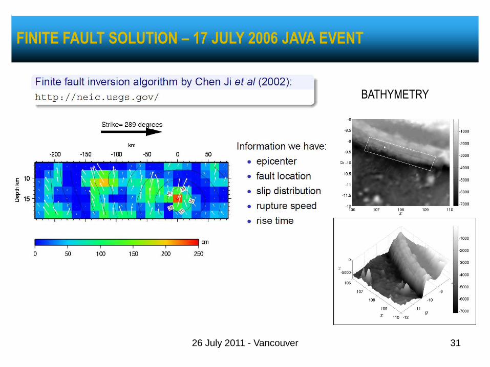
MATHEMATICAL GENERATION OF A TSUNAMI (CLASSICAL)

Okada‟s solution (or Mansinha &

Smylie) based on dislocation theory

and fundamental solution for an elastic

half-space

Fault consisting of one or a few

segments (Grilli et al. (2007) for 2004

megatsunami, Yalciner (2008) for Java

2006 event, …)

Passive tsunami generation

Illustration – July 17, 2006 Java event

– single-fault based initial condition


SEA BOTTOM DEFORMATION

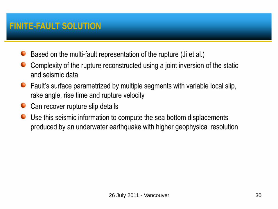
Based on the multi-fault representation of the rupture (Ji et al.)

Complexity of the rupture reconstructed using a joint inversion of the static

and seismic data

Fault‟s surface parametrized by multiple segments with variable local slip,

rake angle, rise time and rupture velocity

Can recover rupture slip details

Use this seismic information to compute the sea bottom displacements

produced by an underwater earthquake with higher geophysical resolution


FINITE-FAULT SOLUTION


FINITE FAULT SOLUTION – 17 JULY 2006 JAVA EVENT

BATHYMETRY

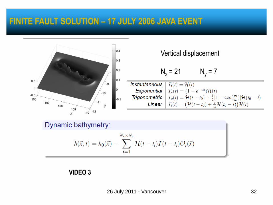
Vertical displacement

Nx = 21 Ny = 7


FINITE FAULT SOLUTION – 17 JULY 2006 JAVA EVENT

VIDEO 3


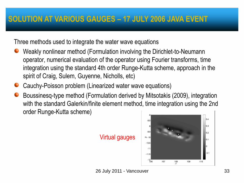
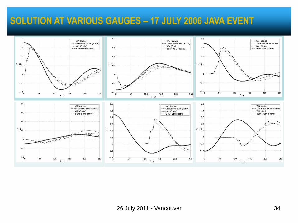
SOLUTION AT VARIOUS GAUGES – 17 JULY 2006 JAVA EVENT

Three methods used to integrate the water wave equations

Weakly nonlinear method (Formulation involving the Dirichlet-to-Neumann

operator, numerical evaluation of the operator using Fourier transforms, time

integration using the standard 4th order Runge-Kutta scheme, approach in the

spirit of Craig, Sulem, Guyenne, Nicholls, etc)

Cauchy-Poisson problem (Linearized water wave equations)

Boussinesq-type method (Formulation derived by Mitsotakis (2009), integration

with the standard Galerkin/finite element method, time integration using the 2nd

order Runge-Kutta scheme)

Virtual gauges


SOLUTION AT VARIOUS GAUGES – 17 JULY 2006 JAVA EVENT


OTHER TOPIC IN TSUNAMI RESEARCH – EFFECT OF SEDIMENTS

Science 17 June 2011

As the rupture neared the seafloor, the movement of the fault grew rapidly, violently

deforming the seafloor sediments sitting on top of the fault plane, punching the overlying

water upward and triggering the tsunami.

This amplification of slip near the surface was predicted in computer simulations of

earthquake rupture, but this is the first time we have clearly seen it occur in a real

earthquake.


OTHER TOPIC IN TSUNAMI RESEARCH – EFFECT OF SEDIMENTS

sediment thickness / fault depth

amplification

0 0.25

80%


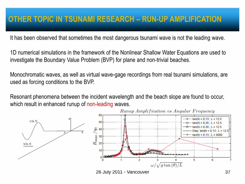
OTHER TOPIC IN TSUNAMI RESEARCH – RUN-UP AMPLIFICATION

It has been observed that sometimes the most dangerous tsunami wave is not the leading wave.

1D numerical simulations in the framework of the Nonlinear Shallow Water Equations are used to

investigate the Boundary Value Problem (BVP) for plane and non-trivial beaches.

Monochromatic waves, as well as virtual wave-gage recordings from real tsunami simulations, are

used as forcing conditions to the BVP.

Resonant phenomena between the incident wavelength and the beach slope are found to occur,

which result in enhanced runup of non-leading waves.


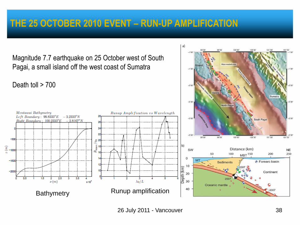
THE 25 OCTOBER 2010 EVENT – RUN-UP AMPLIFICATION

Magnitude 7.7 earthquake on 25 October west of South

Pagai, a small island off the west coast of Sumatra

Death toll > 700

Bathymetry Runup amplification


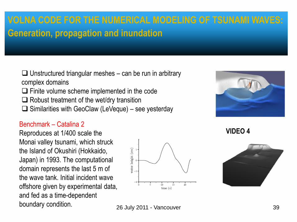
VOLNA CODE FOR THE NUMERICAL MODELING OF TSUNAMI WAVES:

Generation, propagation and inundation

Unstructured triangular meshes – can be run in arbitrary

complex domains

Finite volume scheme implemented in the code

Robust treatment of the wet/dry transition

Similarities with GeoClaw (LeVeque) – see yesterday

Benchmark – Catalina 2

Reproduces at 1/400 scale the

Monai valley tsunami, which struck

the Island of Okushiri (Hokkaido,

Japan) in 1993. The computational

domain represents the last 5 m of

the wave tank. Initial incident wave

offshore given by experimental data,

and fed as a time-dependent

boundary condition.

VIDEO 4

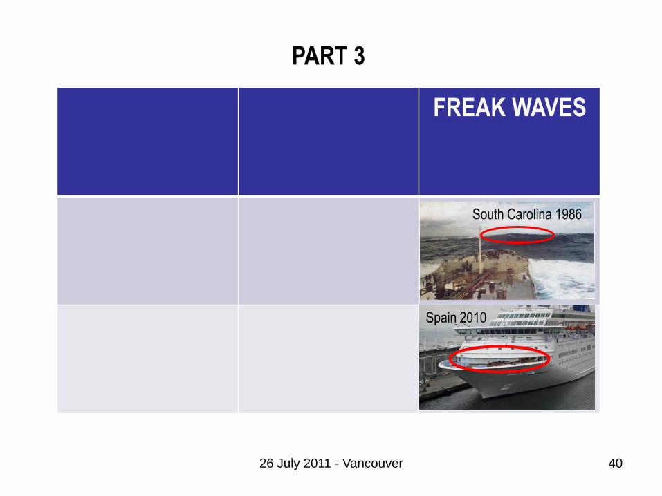
PART 3

FREAK WAVES

South Carolina 1986

Spain 2010


EXTREME OCEAN WAVES

Rogue Waves are large oceanic surface waves that represent statistically-rare

wave height outliers

Damage and fatalities when wave height is outside design criteria

1934

26 July 2011 - Vancouver 41

February 1986 - It was a nice day with light breezes and

no significant sea. Only the long swell, about 5 m high

and 200 to 300 m long. We were on the wing of the

bridge, with a height of eye of 17 m, and this wave broke

over our heads. Shot taken while diving down off the

face of the second of a set of three waves. Foremast

was bent back about 20 degrees (Captain A. Chase)

Foremast

EXTREME OCEAN WAVES

Definition of a Rogue Wave: H / Hs > 2 where H is the wave height (trough to

crest) and Hs the significant wave height (average wave height of the one-third

largest waves)

Rogue waves are localised in space (order of 1 km) and in time (order of 1 minute)

Existence confirmed in 1990‟s through long term wave height measurements and

specific events (oil platform measurements)

Draupner 1995


Time in seconds

Elevation of the sea

surface in metres

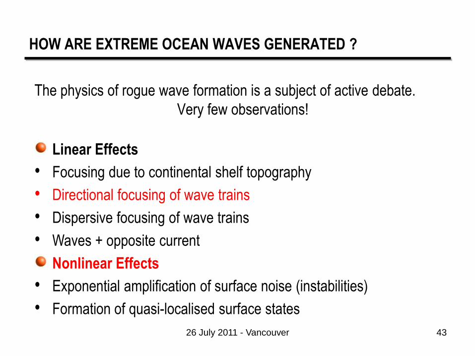
The physics of rogue wave formation is a subject of active debate.

Very few observations!

Linear Effects

• Focusing due to continental shelf topography

• Directional focusing of wave trains

• Dispersive focusing of wave trains

• Waves + opposite current

Nonlinear Effects

• Exponential amplification of surface noise (instabilities)

• Formation of quasi-localised surface states

HOW ARE EXTREME OCEAN WAVES GENERATED ?


The physics of rogue wave formation is a subject of active debate and studies are

not helped by practical observational difficulties

EXTREME OCEAN WAVES

Observation of swell propagation from satellite

data (IFREMER, BOOst Technologies)

Evidence of directional wave focusing in

a « numerical » wave tank (Fochesato,

Grilli, Dias, Wave Motion, 2007 – based

on BEM)


VIDEO 5 –

Experiments in

Nantes

NONLINEAR EFFECTS – NONLINEAR SCHRÖDINGER EQUATION


What does the Nonlinear Schrödinger equation contain? (Osborne‟s book)

(1) The superposition of weakly nonlinear Fourier components.

(2) The Stokes wave nonlinearity.

(3) The modulational instability.

Two populations of nonlinear waves:

Population 1: Weakly nonlinear superposition of sine waves (1) together with the Stokes-

wave correction (2).

Population 2: Item (3) predicts the existence of unstable wave packets, which can rise up

to more than twice the significant wave height.

Unstable packets are a type of nonlinear Fourier component in NLS spectral theory. This

spectral contribution arises from the Benjamin-Feir instability and obeys a threshold effect:

Only large enough wave fields have unstable modes in the spectrum.

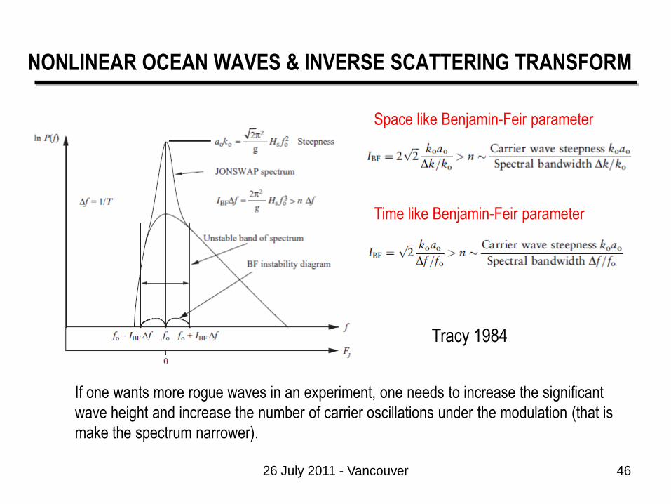
NONLINEAR OCEAN WAVES & INVERSE SCATTERING TRANSFORM


Space like Benjamin-Feir parameter

Time like Benjamin-Feir parameter

If one wants more rogue waves in an experiment, one needs to increase the significant

wave height and increase the number of carrier oscillations under the modulation (that is

make the spectrum narrower).

Tracy 1984

EXTREME WAVES GENERATED BY MODULATIONAL INSTABILITY

The initial wave condition is a monochromatic deep water wave with a small disturbance added

(modulation with a wavelength much larger than the wavelength of the carrier).

After several wave periods instabilities develop and energy becomes concentrated at a single

peak in the wave group.


Snapshots of the surface elevation

during 10 wave periods

Surface elevation in a time-

space representation (during

10 wave periods)

T.B. Benjamin

1929

-1995

MODULATION INSTABILITY IN THE TIME NLSE

Exponential growth of a periodic perturbation

Linear stability analysis yields gain, etc


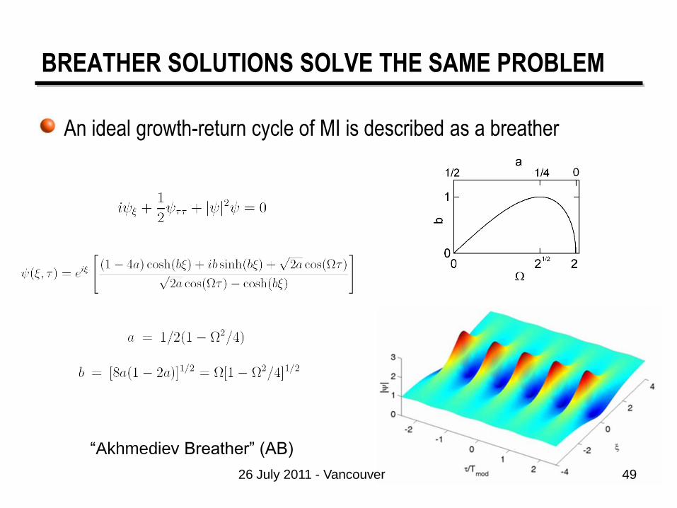
An ideal growth-return cycle of MI is described as a breather

“Akhmediev Breather” (AB)

BREATHER SOLUTIONS SOLVE THE SAME PROBLEM


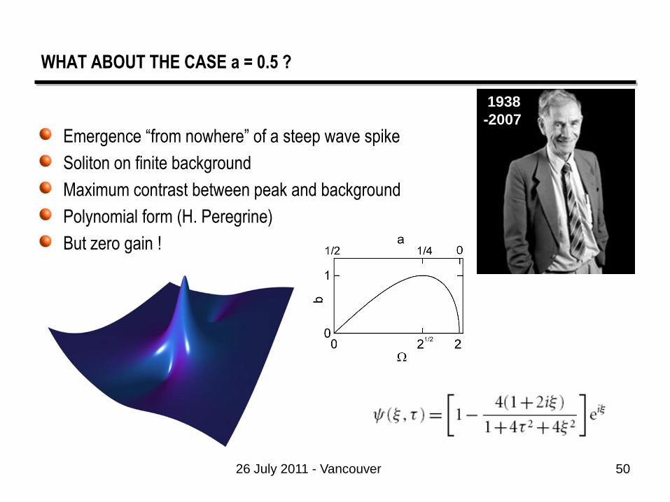
WHAT ABOUT THE CASE a = 0.5 ?

Emergence “from nowhere” of a steep wave spike

Soliton on finite background

Maximum contrast between peak and background

Polynomial form (H. Peregrine)

But zero gain !

1938

-2007


1938

-2007

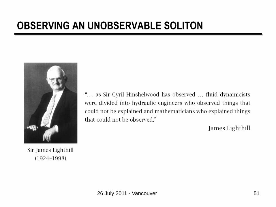
OBSERVING AN UNOBSERVABLE SOLITON


UNDER INDUCED CONDITIONS OUR TEAM FOUND THIS ROGUE WAVE SOLUTION


VIDEO 6

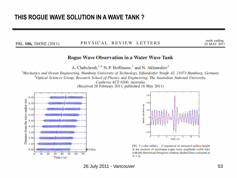
THIS ROGUE WAVE SOLUTION IN A WAVE TANK ?


READING


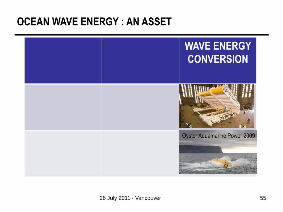
OCEAN WAVE ENERGY : AN ASSET


WAVE ENERGY

CONVERSION

Oyster Aquamarine Power 2009

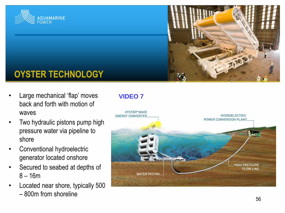
• Large mechanical „flap‟ moves

back and forth with motion of

waves

• Two hydraulic pistons pump high

pressure water via pipeline to

shore

• Conventional hydroelectric

generator located onshore

• Secured to seabed at depths of

8 – 16m

• Located near shore, typically 500

– 800m from shoreline

OYSTER TECHNOLOGY

56

VIDEO 7

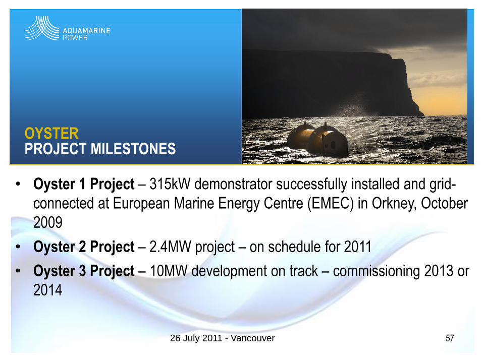
OYSTERPROJECT MILESTONES

• Oyster 1 Project – 315kW demonstrator successfully installed and grid-

connected at European Marine Energy Centre (EMEC) in Orkney, October

2009

• Oyster 2 Project – 2.4MW project – on schedule for 2011

• Oyster 3 Project – 10MW development on track – commissioning 2013 or

2014


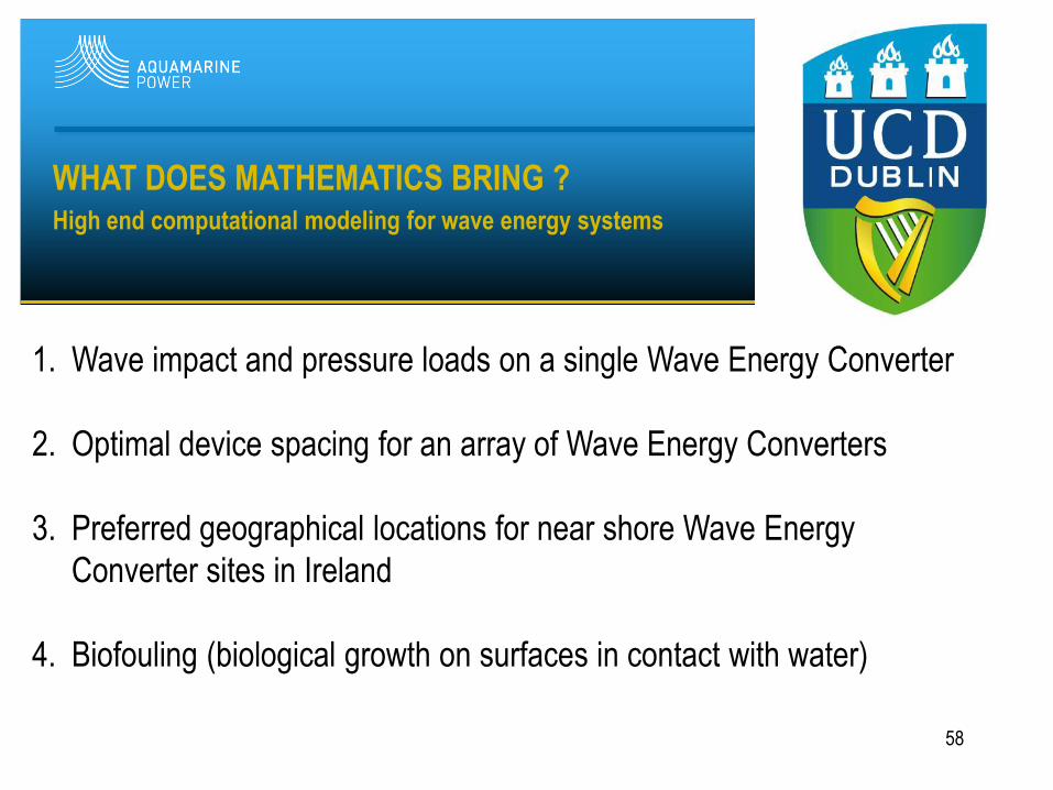
1. Wave impact and pressure loads on a single Wave Energy Converter

2. Optimal device spacing for an array of Wave Energy Converters

3. Preferred geographical locations for near shore Wave Energy

Converter sites in Ireland

4. Biofouling (biological growth on surfaces in contact with water)

WHAT DOES MATHEMATICS BRING ?High end computational modeling for wave energy systems

58

• One of the most commonly acknowledged

difficulties of conducting experiments with

Wave Energy Converters : presence of

scale effects (Reynolds much larger at full

scale than at small scale – for example, at

scale 1/40, viscous forces on the model

are multiplied by a factor 253 if only

Froude scaling is satisfied)

• This makes mathematical and numerical

modelling a particularly valuable tool in the

development of Wave Energy Converters

SURVIVABILITY

Scale effects in experiments at small scale

59

Experiments performed at Queen‟s University Belfast

CONCLUDING REMARKS


Flaps might be simple devices from the engineering point of view. But they are really

challenging from the fluid mechanics and numerical simulation points of view

•Intermediate water depth (kh of order unity)

•3D problem

•Neither laminar flow nor potential flow (vortex shedding)

•Moving solid boundary (large motion) + free surface

•Intermediate size structure (no simplification)

•Nonlinear waves

•Coupling with biological growth

THANK YOU FOR YOUR ATTENTION

MERCI POUR VOTRE ATTENTION


Howth, Ireland

THE NUMERICAL COMPUTATION OF VIOLENT WAVES APPLICATION · PDF fileTHE NUMERICAL COMPUTATION OF...

Documents

Transcript of THE NUMERICAL COMPUTATION OF VIOLENT WAVES APPLICATION · PDF fileTHE NUMERICAL COMPUTATION OF...