
The NLMIXED Procedure - SAS Technical Support | SAS … NLMIXED Compared with Other SAS Procedures...
111
SAS/STAT ® 14.1 User’s Guide The NLMIXED Procedure
Transcript of The NLMIXED Procedure - SAS Technical Support | SAS … NLMIXED Compared with Other SAS Procedures...

SAS/STAT® 14.1 User’s GuideThe NLMIXED Procedure

This document is an individual chapter from SAS/STAT® 14.1 User’s Guide.
The correct bibliographic citation for this manual is as follows: SAS Institute Inc. 2015. SAS/STAT® 14.1 User’s Guide. Cary, NC:SAS Institute Inc.
SAS/STAT® 14.1 User’s Guide
Copyright © 2015, SAS Institute Inc., Cary, NC, USA
All Rights Reserved. Produced in the United States of America.
For a hard-copy book: No part of this publication may be reproduced, stored in a retrieval system, or transmitted, in any form or byany means, electronic, mechanical, photocopying, or otherwise, without the prior written permission of the publisher, SAS InstituteInc.
For a web download or e-book: Your use of this publication shall be governed by the terms established by the vendor at the timeyou acquire this publication.
The scanning, uploading, and distribution of this book via the Internet or any other means without the permission of the publisher isillegal and punishable by law. Please purchase only authorized electronic editions and do not participate in or encourage electronicpiracy of copyrighted materials. Your support of others’ rights is appreciated.
U.S. Government License Rights; Restricted Rights: The Software and its documentation is commercial computer softwaredeveloped at private expense and is provided with RESTRICTED RIGHTS to the United States Government. Use, duplication, ordisclosure of the Software by the United States Government is subject to the license terms of this Agreement pursuant to, asapplicable, FAR 12.212, DFAR 227.7202-1(a), DFAR 227.7202-3(a), and DFAR 227.7202-4, and, to the extent required under U.S.federal law, the minimum restricted rights as set out in FAR 52.227-19 (DEC 2007). If FAR 52.227-19 is applicable, this provisionserves as notice under clause (c) thereof and no other notice is required to be affixed to the Software or documentation. TheGovernment’s rights in Software and documentation shall be only those set forth in this Agreement.
SAS Institute Inc., SAS Campus Drive, Cary, NC 27513-2414
July 2015
SAS® and all other SAS Institute Inc. product or service names are registered trademarks or trademarks of SAS Institute Inc. in theUSA and other countries. ® indicates USA registration.
Other brand and product names are trademarks of their respective companies.
Chapter 82
The NLMIXED Procedure
ContentsOverview: NLMIXED Procedure . . . . . . . . . . . . . . . . . . . . . . . . . . . . . . . 6518
Introduction . . . . . . . . . . . . . . . . . . . . . . . . . . . . . . . . . . . . . . . 6518Literature on Nonlinear Mixed Models . . . . . . . . . . . . . . . . . . . . . . . . . 6518PROC NLMIXED Compared with Other SAS Procedures and Macros . . . . . . . . 6519
Getting Started: NLMIXED Procedure . . . . . . . . . . . . . . . . . . . . . . . . . . . . . 6520Nonlinear Growth Curves with Gaussian Data . . . . . . . . . . . . . . . . . . . . . 6520Logistic-Normal Model with Binomial Data . . . . . . . . . . . . . . . . . . . . . . 6523
Syntax: NLMIXED Procedure . . . . . . . . . . . . . . . . . . . . . . . . . . . . . . . . . 6527PROC NLMIXED Statement . . . . . . . . . . . . . . . . . . . . . . . . . . . . . . 6527ARRAY Statement . . . . . . . . . . . . . . . . . . . . . . . . . . . . . . . . . . . . 6545BOUNDS Statement . . . . . . . . . . . . . . . . . . . . . . . . . . . . . . . . . . . 6546BY Statement . . . . . . . . . . . . . . . . . . . . . . . . . . . . . . . . . . . . . . 6546CONTRAST Statement . . . . . . . . . . . . . . . . . . . . . . . . . . . . . . . . . 6547ESTIMATE Statement . . . . . . . . . . . . . . . . . . . . . . . . . . . . . . . . . . 6547ID Statement . . . . . . . . . . . . . . . . . . . . . . . . . . . . . . . . . . . . . . . 6547MODEL Statement . . . . . . . . . . . . . . . . . . . . . . . . . . . . . . . . . . . . 6548PARMS Statement . . . . . . . . . . . . . . . . . . . . . . . . . . . . . . . . . . . . 6548PREDICT Statement . . . . . . . . . . . . . . . . . . . . . . . . . . . . . . . . . . . 6549RANDOM Statement . . . . . . . . . . . . . . . . . . . . . . . . . . . . . . . . . . 6550REPLICATE Statement . . . . . . . . . . . . . . . . . . . . . . . . . . . . . . . . . 6551Programming Statements . . . . . . . . . . . . . . . . . . . . . . . . . . . . . . . . 6551
Details: NLMIXED Procedure . . . . . . . . . . . . . . . . . . . . . . . . . . . . . . . . . 6553Modeling Assumptions and Notation . . . . . . . . . . . . . . . . . . . . . . . . . . 6553Integral Approximations . . . . . . . . . . . . . . . . . . . . . . . . . . . . . . . . . 6555Built-in Log-Likelihood Functions . . . . . . . . . . . . . . . . . . . . . . . . . . . 6557Hierarchical Model Specification . . . . . . . . . . . . . . . . . . . . . . . . . . . . 6559Optimization Algorithms . . . . . . . . . . . . . . . . . . . . . . . . . . . . . . . . . 6561Finite-Difference Approximations of Derivatives . . . . . . . . . . . . . . . . . . . . 6566Hessian Scaling . . . . . . . . . . . . . . . . . . . . . . . . . . . . . . . . . . . . . 6568Active Set Methods . . . . . . . . . . . . . . . . . . . . . . . . . . . . . . . . . . . 6568Line-Search Methods . . . . . . . . . . . . . . . . . . . . . . . . . . . . . . . . . . 6570Restricting the Step Length . . . . . . . . . . . . . . . . . . . . . . . . . . . . . . . 6571Computational Problems . . . . . . . . . . . . . . . . . . . . . . . . . . . . . . . . . 6572Covariance Matrix . . . . . . . . . . . . . . . . . . . . . . . . . . . . . . . . . . . . 6575Prediction . . . . . . . . . . . . . . . . . . . . . . . . . . . . . . . . . . . . . . . . 6576Computational Resources . . . . . . . . . . . . . . . . . . . . . . . . . . . . . . . . 6576
6518 F Chapter 82: The NLMIXED Procedure
Displayed Output . . . . . . . . . . . . . . . . . . . . . . . . . . . . . . . . . . . . . 6577ODS Table Names . . . . . . . . . . . . . . . . . . . . . . . . . . . . . . . . . . . . 6580
Examples: NLMIXED Procedure . . . . . . . . . . . . . . . . . . . . . . . . . . . . . . . 6580Example 82.1: One-Compartment Model with Pharmacokinetic Data . . . . . . . . . 6580Example 82.2: Probit-Normal Model with Binomial Data . . . . . . . . . . . . . . . 6584Example 82.3: Probit-Normal Model with Ordinal Data . . . . . . . . . . . . . . . . 6587Example 82.4: Poisson-Normal Model with Count Data . . . . . . . . . . . . . . . . 6591Example 82.5: Failure Time and Frailty Model . . . . . . . . . . . . . . . . . . . . . 6594Example 82.6: Simulated Nested Linear Random-Effects Model . . . . . . . . . . . . 6604Example 82.7: Overdispersion Hierarchical Nonlinear Mixed Model . . . . . . . . . . 6607
References . . . . . . . . . . . . . . . . . . . . . . . . . . . . . . . . . . . . . . . . . . . 6613
Overview: NLMIXED Procedure
IntroductionThe NLMIXED procedure fits nonlinear mixed models—that is, models in which both fixed and randomeffects enter nonlinearly. These models have a wide variety of applications, two of the most common beingpharmacokinetics and overdispersed binomial data. PROC NLMIXED enables you to specify a conditionaldistribution for your data (given the random effects) having either a standard form (normal, binomial, Poisson)or a general distribution that you code using SAS programming statements.
PROC NLMIXED fits nonlinear mixed models by maximizing an approximation to the likelihood integratedover the random effects. Different integral approximations are available, the principal ones being adaptiveGaussian quadrature and a first-order Taylor series approximation. A variety of alternative optimizationtechniques are available to carry out the maximization; the default is a dual quasi-Newton algorithm.
Successful convergence of the optimization problem results in parameter estimates along with their approxi-mate standard errors based on the second derivative matrix of the likelihood function. PROC NLMIXEDenables you to use the estimated model to construct predictions of arbitrary functions by using empiricalBayes estimates of the random effects. You can also estimate arbitrary functions of the nonrandom parameters,and PROC NLMIXED computes their approximate standard errors by using the delta method.
Literature on Nonlinear Mixed ModelsDavidian and Giltinan (1995) and Vonesh and Chinchilli (1997) provide good overviews as well as generaltheoretical developments and examples of nonlinear mixed models. Pinheiro and Bates (1995) is a primaryreference for the theory and computational techniques of PROC NLMIXED. They describe and compareseveral different integrated likelihood approximations and provide evidence that adaptive Gaussian quadratureis one of the best methods. Davidian and Gallant (1993) also use Gaussian quadrature for nonlinear mixedmodels, although the smooth nonparametric density they advocate for the random effects is currently notavailable in PROC NLMIXED.

PROC NLMIXED Compared with Other SAS Procedures and Macros F 6519
Traditional approaches to fitting nonlinear mixed models involve Taylor series expansions, expanding aroundeither zero or the empirical best linear unbiased predictions of the random effects. The former is the basis forthe well-known first-order method (Beal and Sheiner 1982, 1988; Sheiner and Beal 1985), and it is optionallyavailable in PROC NLMIXED. The latter is the basis for the estimation method of Lindstrom and Bates(1990), and it is not available in PROC NLMIXED. However, the closely related Laplacian approximation isan option; it is equivalent to adaptive Gaussian quadrature with only one quadrature point. The Laplacianapproximation and its relationship to the Lindstrom-Bates method are discussed by: Beal and Sheiner (1992);Wolfinger (1993); Vonesh (1992, 1996); Vonesh and Chinchilli (1997); Wolfinger and Lin (1997).
A parallel literature exists in the area of generalized linear mixed models, in which random effects appearas a part of the linear predictor inside a link function. Taylor-series methods similar to those just describedare discussed in articles such as: Harville and Mee (1984); Stiratelli, Laird, and Ware (1984); Gilmour,Anderson, and Rae (1985); Goldstein (1991); Schall (1991); Engel and Keen (1992); Breslow and Clayton(1993); Wolfinger and O’Connell (1993); McGilchrist (1994), but such methods have not been implementedin PROC NLMIXED because they can produce biased results in certain binary data situations (Rodriguezand Goldman 1995; Lin and Breslow 1996). Instead, a numerical quadrature approach is available in PROCNLMIXED, as discussed in: Pierce and Sands (1975); Anderson and Aitkin (1985); Hedeker and Gibbons(1994); Crouch and Spiegelman (1990); Longford (1994); McCulloch (1994); Liu and Pierce (1994); Diggle,Liang, and Zeger (1994).
Nonlinear mixed models have important applications in pharmacokinetics, and Roe (1997) provides a wide-ranging comparison of many popular techniques. Yuh et al. (1994) provide an extensive bibliography onnonlinear mixed models and their use in pharmacokinetics.
PROC NLMIXED Compared with Other SAS Procedures and MacrosThe models fit by PROC NLMIXED can be viewed as generalizations of the random coefficient models fit bythe MIXED procedure. This generalization allows the random coefficients to enter the model nonlinearly,whereas in PROC MIXED they enter linearly. With PROC MIXED you can perform both maximumlikelihood and restricted maximum likelihood (REML) estimation, whereas PROC NLMIXED implementsonly maximum likelihood. This is because the analog to the REML method in PROC NLMIXED wouldinvolve a high-dimensional integral over all of the fixed-effects parameters, and this integral is typically notavailable in closed form. Finally, PROC MIXED assumes the data to be normally distributed, whereas PROCNLMIXED enables you to analyze data that are normal, binomial, or Poisson or that have any likelihoodprogrammable with SAS statements.
PROC NLMIXED does not implement the same estimation techniques available with the NLINMIX macroor the default estimation method of the GLIMMIX procedure. These are based on the estimation methodsof: Lindstrom and Bates (1990); Breslow and Clayton (1993); Wolfinger and O’Connell (1993), and theyiteratively fit a set of generalized estimating equations (see Chapters 14 and 15 of Littell et al. 2006; Wolfinger1997). In contrast, PROC NLMIXED directly maximizes an approximate integrated likelihood. This remarkalso applies to the SAS/IML macros MIXNLIN (Vonesh and Chinchilli 1997) and NLMEM (Galecki 1998).
The GLIMMIX procedure also fits mixed models for nonnormal data with nonlinearity in the conditionalmean function. In contrast to the NLMIXED procedure, PROC GLIMMIX assumes that the model containsa linear predictor that links covariates to the conditional mean of the response. The NLMIXED procedureis designed to handle general conditional mean functions, whether they contain a linear component ornot. As mentioned earlier, the GLIMMIX procedure by default estimates parameters in generalized linearmixed models by pseudo-likelihood techniques, whereas PROC NLMIXED by default performs maximum

6520 F Chapter 82: The NLMIXED Procedure
likelihood estimation by adaptive Gauss-Hermite quadrature. This estimation method is also available withthe GLIMMIX procedure (METHOD=QUAD in the PROC GLIMMIX statement).
PROC NLMIXED has close ties with the NLP procedure in SAS/OR software. PROC NLMIXED uses asubset of the optimization code underlying PROC NLP and has many of the same optimization-based options.Also, the programming statement functionality used by PROC NLMIXED is the same as that used by PROCNLP and the MODEL procedure in SAS/ETS software.
Getting Started: NLMIXED Procedure
Nonlinear Growth Curves with Gaussian DataAs an introductory example, consider the orange tree data of Draper and Smith (1981). These data consist ofseven measurements of the trunk circumference (in millimeters) on each of five orange trees. You can inputthese data into a SAS data set as follows:
data tree;input tree day y;datalines;
1 118 301 484 581 664 87
... more lines ...
5 1582 177;
Lindstrom and Bates (1990) and Pinheiro and Bates (1995) propose the following logistic nonlinear mixedmodel for these data:
yij Db1 C ui1
1C expŒ�.dij � b2/=b3�C eij
Here, yij represents the jth measurement on the ith tree (i D 1; : : : ; 5; j D 1; : : : ; 7), dij is the correspondingday, b1; b2; b3 are the fixed-effects parameters, ui1 are the random-effect parameters assumed to be iidN.0; �2u/, and eij are the residual errors assumed to be iid N.0; �2e / and independent of the ui1. This modelhas a logistic form, and the random-effect parameters ui1 enter the model linearly.
The statements to fit this nonlinear mixed model are as follows:
proc nlmixed data=tree;parms b1=190 b2=700 b3=350 s2u=1000 s2e=60;num = b1+u1;ex = exp(-(day-b2)/b3);den = 1 + ex;model y ~ normal(num/den,s2e);random u1 ~ normal(0,s2u) subject=tree;
run;

Nonlinear Growth Curves with Gaussian Data F 6521
The PROC NLMIXED statement invokes the procedure and inputs the tree data set. The PARMS statementidentifies the unknown parameters and their starting values. Here there are three fixed-effects parameters (b1,b2, b3) and two variance components (s2u, s2e).
The next three statements are SAS programming statements specifying the logistic mixed model. A newvariable u1 is included to identify the random effect. These statements are evaluated for every observation inthe data set when the NLMIXED procedure computes the log likelihood function and its derivatives.
The MODEL statement defines the dependent variable and its conditional distribution given the randomeffects. Here a normal (Gaussian) conditional distribution is specified with mean num/den and variance s2e.
The RANDOM statement defines the single random effect to be u1, and specifies that it follow a normaldistribution with mean 0 and variance s2u. The SUBJECT= argument in the RANDOM statement defines avariable indicating when the random effect obtains new realizations; in this case, it changes according to thevalues of the tree variable. PROC NLMIXED assumes that the input data set is clustered according to thelevels of the tree variable; that is, all observations from the same tree occur sequentially in the input data set.
The output from this analysis is as follows.
Figure 82.1 Model Specifications
The NLMIXED ProcedureThe NLMIXED Procedure
Specifications
Data Set WORK.TREE
Dependent Variable y
Distribution for Dependent Variable Normal
Random Effects u1
Distribution for Random Effects Normal
Subject Variable tree
Optimization Technique Dual Quasi-Newton
Integration Method Adaptive Gaussian Quadrature
The “Specifications” table lists basic information about the nonlinear mixed model you have specified(Figure 82.1). Included are the input data set, the dependent and subject variables, the random effects, therelevant distributions, and the type of optimization. The “Dimensions” table lists various counts related to themodel, including the number of observations, subjects, and parameters (Figure 82.2). These quantities areuseful for checking that you have specified your data set and model correctly. Also listed is the number ofquadrature points that PROC NLMIXED has selected based on the evaluation of the log likelihood at thestarting values of the parameters. Here, only one quadrature point is necessary because the random-effectparameters ui1 enter the model linearly. (The Gauss-Hermite quadrature with a single quadrature pointresults in the Laplace approximation of the log likelihood.)
6522 F Chapter 82: The NLMIXED Procedure
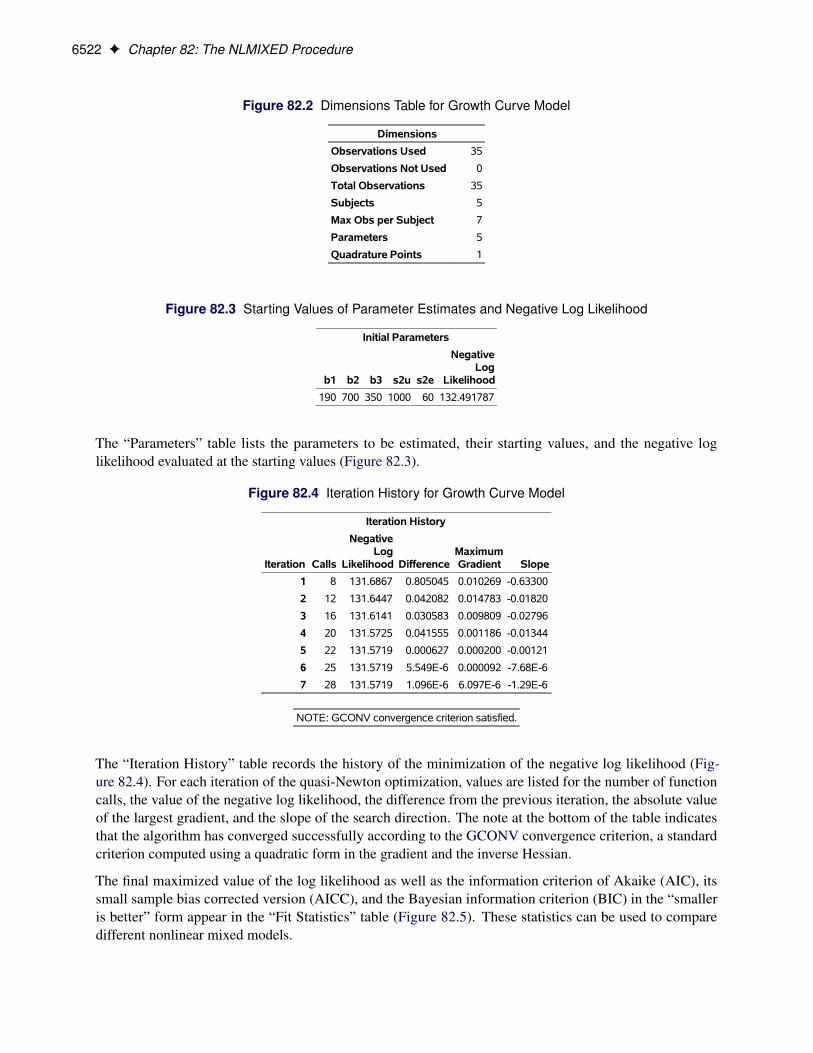
Figure 82.2 Dimensions Table for Growth Curve Model
Dimensions
Observations Used 35
Observations Not Used 0
Total Observations 35
Subjects 5
Max Obs per Subject 7
Parameters 5
Quadrature Points 1
Figure 82.3 Starting Values of Parameter Estimates and Negative Log Likelihood
Initial Parameters
b1 b2 b3 s2u s2e
NegativeLog
Likelihood
190 700 350 1000 60 132.491787
The “Parameters” table lists the parameters to be estimated, their starting values, and the negative loglikelihood evaluated at the starting values (Figure 82.3).
Figure 82.4 Iteration History for Growth Curve Model
Iteration History
Iteration Calls
NegativeLog
Likelihood DifferenceMaximumGradient Slope
1 8 131.6867 0.805045 0.010269 -0.63300
2 12 131.6447 0.042082 0.014783 -0.01820
3 16 131.6141 0.030583 0.009809 -0.02796
4 20 131.5725 0.041555 0.001186 -0.01344
5 22 131.5719 0.000627 0.000200 -0.00121
6 25 131.5719 5.549E-6 0.000092 -7.68E-6
7 28 131.5719 1.096E-6 6.097E-6 -1.29E-6
NOTE: GCONV convergence criterion satisfied.
The “Iteration History” table records the history of the minimization of the negative log likelihood (Fig-ure 82.4). For each iteration of the quasi-Newton optimization, values are listed for the number of functioncalls, the value of the negative log likelihood, the difference from the previous iteration, the absolute valueof the largest gradient, and the slope of the search direction. The note at the bottom of the table indicatesthat the algorithm has converged successfully according to the GCONV convergence criterion, a standardcriterion computed using a quadratic form in the gradient and the inverse Hessian.
The final maximized value of the log likelihood as well as the information criterion of Akaike (AIC), itssmall sample bias corrected version (AICC), and the Bayesian information criterion (BIC) in the “smalleris better” form appear in the “Fit Statistics” table (Figure 82.5). These statistics can be used to comparedifferent nonlinear mixed models.

Logistic-Normal Model with Binomial Data F 6523
Figure 82.5 Fit Statistics for Growth Curve Model
Fit Statistics
-2 Log Likelihood 263.1
AIC (smaller is better) 273.1
AICC (smaller is better) 275.2
BIC (smaller is better) 271.2
Figure 82.6 Parameter Estimates at Convergence
Parameter Estimates
Parameter EstimateStandard
Error DF t Value Pr > |t|
95%Confidence
Limits Gradient
b1 192.05 15.6473 4 12.27 0.0003 148.61 235.50 1.154E-6
b2 727.90 35.2474 4 20.65 <.0001 630.04 825.76 5.289E-6
b3 348.07 27.0793 4 12.85 0.0002 272.88 423.25 -6.1E-6
s2u 999.88 647.44 4 1.54 0.1974 -797.71 2797.46 -3.84E-6
s2e 61.5139 15.8832 4 3.87 0.0179 17.4150 105.61 2.892E-6
The maximum likelihood estimates of the five parameters and their approximate standard errors computedusing the final Hessian matrix are displayed in the “Parameter Estimates” table (Figure 82.6). Approximatet-values and Wald-type confidence limits are also provided, with degrees of freedom equal to the number ofsubjects minus the number of random effects. You should interpret these statistics cautiously for varianceparameters like s2u and s2e. The final column in the output shows the gradient vector at the optimizationsolution. Each element appears to be sufficiently small to indicate a stationary point.
Since the random-effect parameters ui1 enter the model linearly, you can obtain equivalent results by usingthe first-order method (specify METHOD=FIRO in the PROC NLMIXED statement).
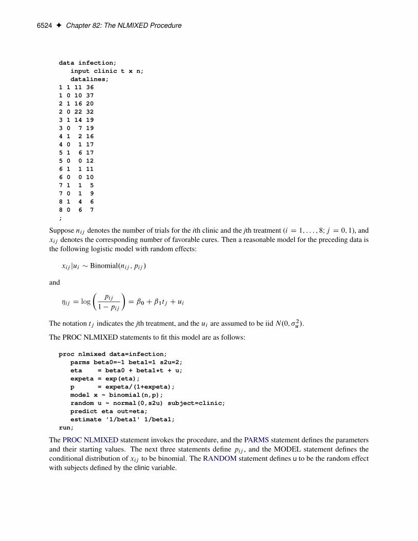
Logistic-Normal Model with Binomial DataThis example analyzes the data from Beitler and Landis (1985), which represent results from a multi-centerclinical trial investigating the effectiveness of two topical cream treatments (active drug, control) in curing aninfection. For each of eight clinics, the number of trials and favorable cures are recorded for each treatment.The SAS data set is as follows.
6524 F Chapter 82: The NLMIXED Procedure
data infection;input clinic t x n;datalines;
1 1 11 361 0 10 372 1 16 202 0 22 323 1 14 193 0 7 194 1 2 164 0 1 175 1 6 175 0 0 126 1 1 116 0 0 107 1 1 57 0 1 98 1 4 68 0 6 7;
Suppose nij denotes the number of trials for the ith clinic and the jth treatment (i D 1; : : : ; 8I j D 0; 1), andxij denotes the corresponding number of favorable cures. Then a reasonable model for the preceding data isthe following logistic model with random effects:
xij jui � Binomial.nij ; pij /
and
�ij D log�
pij
1 � pij
�D ˇ0 C ˇ1tj C ui
The notation tj indicates the jth treatment, and the ui are assumed to be iid N.0; �2u/.
The PROC NLMIXED statements to fit this model are as follows:
proc nlmixed data=infection;parms beta0=-1 beta1=1 s2u=2;eta = beta0 + beta1*t + u;expeta = exp(eta);p = expeta/(1+expeta);model x ~ binomial(n,p);random u ~ normal(0,s2u) subject=clinic;predict eta out=eta;estimate '1/beta1' 1/beta1;
run;
The PROC NLMIXED statement invokes the procedure, and the PARMS statement defines the parametersand their starting values. The next three statements define pij , and the MODEL statement defines theconditional distribution of xij to be binomial. The RANDOM statement defines u to be the random effectwith subjects defined by the clinic variable.

Logistic-Normal Model with Binomial Data F 6525
The PREDICT statement constructs predictions for each observation in the input data set. For this example,predictions of �ij and approximate standard errors of prediction are output to a data set named eta. Thesepredictions include empirical Bayes estimates of the random effects ui .
The ESTIMATE statement requests an estimate of the reciprocal of ˇ1.
The output for this model is as follows.
Figure 82.7 Model Information and Dimensions for Logistic-Normal Model
The NLMIXED ProcedureThe NLMIXED Procedure
Specifications
Data Set WORK.INFECTION
Dependent Variable x
Distribution for Dependent Variable Binomial
Random Effects u
Distribution for Random Effects Normal
Subject Variable clinic
Optimization Technique Dual Quasi-Newton
Integration Method Adaptive Gaussian Quadrature
Dimensions
Observations Used 16
Observations Not Used 0
Total Observations 16
Subjects 8
Max Obs per Subject 2
Parameters 3
Quadrature Points 5
The “Specifications” table provides basic information about the nonlinear mixed model (Figure 82.7). Forexample, the distribution of the response variable, conditional on normally distributed random effects, isbinomial. The “Dimensions” table provides counts of various variables. You should check this table to makesure the data set and model have been entered properly. PROC NLMIXED selects five quadrature points toachieve the default accuracy in the likelihood calculations.
Figure 82.8 Starting Values of Parameter Estimates
Initial Parameters
beta0 beta1 s2u
NegativeLog
Likelihood
-1 1 2 37.5945925
The “Parameters” table lists the starting point of the optimization and the negative log likelihood at thestarting values (Figure 82.8).
6526 F Chapter 82: The NLMIXED Procedure
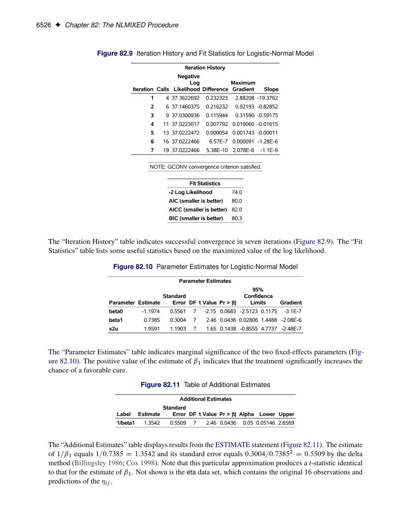
Figure 82.9 Iteration History and Fit Statistics for Logistic-Normal Model
Iteration History
Iteration Calls
NegativeLog
Likelihood DifferenceMaximumGradient Slope
1 4 37.3622692 0.232323 2.88208 -19.3762
2 6 37.1460375 0.216232 0.92193 -0.82852
3 9 37.0300936 0.115944 0.31590 -0.59175
4 11 37.0223017 0.007792 0.019060 -0.01615
5 13 37.0222472 0.000054 0.001743 -0.00011
6 16 37.0222466 6.57E-7 0.000091 -1.28E-6
7 19 37.0222466 5.38E-10 2.078E-6 -1.1E-9
NOTE: GCONV convergence criterion satisfied.
Fit Statistics
-2 Log Likelihood 74.0
AIC (smaller is better) 80.0
AICC (smaller is better) 82.0
BIC (smaller is better) 80.3
The “Iteration History” table indicates successful convergence in seven iterations (Figure 82.9). The “FitStatistics” table lists some useful statistics based on the maximized value of the log likelihood.
Figure 82.10 Parameter Estimates for Logistic-Normal Model
Parameter Estimates
Parameter EstimateStandard
Error DF t Value Pr > |t|
95%Confidence
Limits Gradient
beta0 -1.1974 0.5561 7 -2.15 0.0683 -2.5123 0.1175 -3.1E-7
beta1 0.7385 0.3004 7 2.46 0.0436 0.02806 1.4488 -2.08E-6
s2u 1.9591 1.1903 7 1.65 0.1438 -0.8555 4.7737 -2.48E-7
The “Parameter Estimates” table indicates marginal significance of the two fixed-effects parameters (Fig-ure 82.10). The positive value of the estimate of ˇ1 indicates that the treatment significantly increases thechance of a favorable cure.
Figure 82.11 Table of Additional Estimates
Additional Estimates
Label EstimateStandard
Error DF t Value Pr > |t| Alpha Lower Upper
1/beta1 1.3542 0.5509 7 2.46 0.0436 0.05 0.05146 2.6569
The “Additional Estimates” table displays results from the ESTIMATE statement (Figure 82.11). The estimateof 1=ˇ1 equals 1=0:7385 D 1:3542 and its standard error equals 0:3004=0:73852 D 0:5509 by the deltamethod (Billingsley 1986; Cox 1998). Note that this particular approximation produces a t-statistic identicalto that for the estimate of ˇ1. Not shown is the eta data set, which contains the original 16 observations andpredictions of the �ij .
Syntax: NLMIXED Procedure F 6527
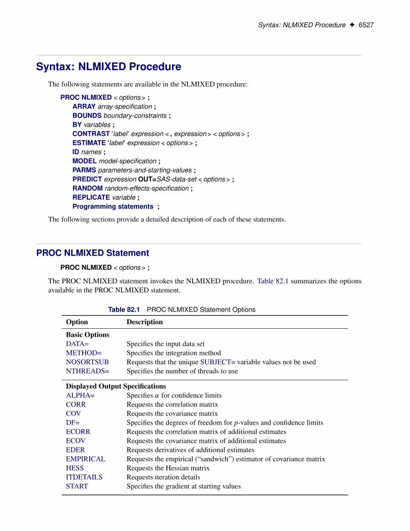
Syntax: NLMIXED ProcedureThe following statements are available in the NLMIXED procedure:
PROC NLMIXED < options > ;ARRAY array-specification ;BOUNDS boundary-constraints ;BY variables ;CONTRAST 'label ' expression < , expression > < options > ;ESTIMATE 'label ' expression < options > ;ID names ;MODEL model-specification ;PARMS parameters-and-starting-values ;PREDICT expression OUT=SAS-data-set < options > ;RANDOM random-effects-specification ;REPLICATE variable ;Programming statements ;
The following sections provide a detailed description of each of these statements.
PROC NLMIXED StatementPROC NLMIXED < options > ;
The PROC NLMIXED statement invokes the NLMIXED procedure. Table 82.1 summarizes the optionsavailable in the PROC NLMIXED statement.
Table 82.1 PROC NLMIXED Statement Options
Option Description
Basic OptionsDATA= Specifies the input data setMETHOD= Specifies the integration methodNOSORTSUB Requests that the unique SUBJECT= variable values not be usedNTHREADS= Specifies the number of threads to use
Displayed Output SpecificationsALPHA= Specifies ˛ for confidence limitsCORR Requests the correlation matrixCOV Requests the covariance matrixDF= Specifies the degrees of freedom for p-values and confidence limitsECORR Requests the correlation matrix of additional estimatesECOV Requests the covariance matrix of additional estimatesEDER Requests derivatives of additional estimatesEMPIRICAL Requests the empirical (“sandwich”) estimator of covariance matrixHESS Requests the Hessian matrixITDETAILS Requests iteration detailsSTART Specifies the gradient at starting values

6528 F Chapter 82: The NLMIXED Procedure
Table 82.1 continued
Option Description
Debugging OutputFLOW Displays the model execution messagesLISTCODE Displays compiled model programLISTDEP Produces a model dependency listingLISTDER Displays the model derivativesLIST Displays the model program and variablesTRACE Displays detailed model execution messagesXREF Displays the model cross references
Quadrature OptionsNOADSCALE Requests no adaptive scalingNOAD Requests no adaptive centeringOUTQ= Displays output data setQFAC= Specifies the search factorQMAX= Specifies the maximum pointsQPOINTS= Specifies the number of pointsQSCALEFAC= Specifies the scale factorQTOL= Specifies the tolerance
Empirical Bayes OptionsEBOPT Requests comprehensive optimizationEBSSFRAC= Specifies the step-shortening fractionEBSSTOL= Specifies the step-shortening toleranceEBSTEPS= Specifies the number of Newton stepsEBSUBSTEPS= Specifies the number of substepsEBTOL= Specifies the convergence toleranceEBZSTART Requests zero as the starting valuesOUTR= Displays an output data set that contains empirical Bayes estimates of
random effects and their approximate standard errors
Optimization SpecificationsHESCAL= Specifies the type of Hessian scalingINHESSIAN<=> Specifies the start for approximated HessianLINESEARCH= Specifies the line-search methodLSPRECISION= Specifies the line-search precisionOPTCHECK<=> Checks optimality in a neighborhoodRESTART= Specifies the iteration number for update restartTECHNIQUE= Specifies the minimization techniqueUPDATE= Specifies the update technique
Derivatives SpecificationsDIAHES Uses only the diagonal of HessianFDHESSIAN<=> Specifies the finite-difference second derivativesFD<=> Specifies the finite-difference derivatives

PROC NLMIXED Statement F 6529
Table 82.1 continued
Option Description
Constraint SpecificationsLCDEACT= Specifies the Lagrange multiplier tolerance for deactivatingLCEPSILON= Specifies the range for active constraintsLCSINGULAR= Specifies the tolerance for dependent constraints
Termination Criteria SpecificationsABSCONV= Specifies the absolute function convergence criterionABSFCONV= Specifies the absolute function difference convergence criterionABSGCONV= Specifies the absolute gradient convergence criterionABSXCONV= Specifies the absolute parameter convergence criterionFCONV= Specifies the relative function convergence criterionFCONV2= Specifies another relative function convergence criterionFDIGITS= Specifies the number accurate digits in objective functionFSIZE= Specifies the FSIZE parameter of the relative function and relative gradient
termination criteriaGCONV= Specifies the relative gradient convergence criterionMAXFUNC= Specifies the maximum number of function callsMAXITER= Specifies the maximum number of iterationsMAXTIME= Specifies the upper limit seconds of CPU timeMINITER= Specifies the minimum number of iterationsXCONV= Specifies the relative parameter convergence criterionXSIZE= Used in XCONV criterion
Step Length SpecificationsDAMPSTEP<=> Specifies the damped steps in line searchINSTEP= Specifies the initial trust-region radiusMAXSTEP= Specifies the maximum trust-region radius
Singularity TolerancesSINGCHOL= Specifies the tolerance for Cholesky rootsSINGHESS= Specifies the tolerance for HessianSINGSWEEP= Specifies the tolerance for sweepSINGVAR= Specifies the tolerance for variances
Covariance Matrix TolerancesASINGULAR= Specifies the absolute singularity for inertiaCFACTOR= Specifies the multiplication factor for COV matrixCOVSING= Specifies the tolerance for singular COV matrixG4= Specifies the threshold for Moore-Penrose inverseMSINGULAR= Specifies the relative M singularity for inertiaVSINGULAR= Specifies the relative V singularity for inertia
These options are described in alphabetical order. For a description of the mathematical notation used in thefollowing sections, see the section “Modeling Assumptions and Notation” on page 6553.

6530 F Chapter 82: The NLMIXED Procedure
ABSCONV=rABSTOL=r
specifies an absolute function convergence criterion. For minimization, termination requires f .�.k// �r . The default value of r is the negative square root of the largest double-precision value, which servesonly as a protection against overflows.
ABSFCONV=r< [n] >ABSFTOL=r< [n] >
specifies an absolute function difference convergence criterion. For all techniques except NMSIMP,termination requires a small change of the function value in successive iterations:
jf .�.k�1// � f .�.k//j � r
The same formula is used for the NMSIMP technique, but �.k/ is defined as the vertex with the lowestfunction value, and �.k�1/ is defined as the vertex with the highest function value in the simplex. Thedefault value is r = 0. The optional integer value n specifies the number of successive iterations forwhich the criterion must be satisfied before the process can be terminated.
ABSGCONV=r< [n] >ABSGTOL=r< [n] >
specifies an absolute gradient convergence criterion. Termination requires the maximum absolutegradient element to be small:
maxjjgj .�
.k//j � r
This criterion is not used by the NMSIMP technique. The default value is r = 1E–5. The optionalinteger value n specifies the number of successive iterations for which the criterion must be satisfiedbefore the process can be terminated. If you specify more than one RANDOM statement, the defaultvalue is r = 1E–3.
ABSXCONV=r< [n] >ABSXTOL=r< [n] >
specifies an absolute parameter convergence criterion. For all techniques except NMSIMP, terminationrequires a small Euclidean distance between successive parameter vectors,
k �.k/ � �.k�1/ k2� r
For the NMSIMP technique, termination requires either a small length ˛.k/ of the vertices of a restartsimplex,
˛.k/ � r
or a small simplex size,
ı.k/ � r
where the simplex size ı.k/ is defined as the L1 distance from the simplex vertex �.k/ with the smallestfunction value to the other n simplex points �.k/
l¤ �.k/:
ı.k/ DX
�l¤y
k �.k/
l� �.k/ k1
The default is r = 1E–8 for the NMSIMP technique and r = 0 otherwise. The optional integer value nspecifies the number of successive iterations for which the criterion must be satisfied before the processcan terminate.

PROC NLMIXED Statement F 6531
ALPHA=˛specifies the alpha level to be used in computing confidence limits. The default value is 0.05.
ASINGULAR=r
ASING=rspecifies an absolute singularity criterion for the computation of the inertia (number of positive,negative, and zero eigenvalues) of the Hessian and its projected forms. The default value is the squareroot of the smallest positive double-precision value.
CFACTOR=fspecifies a multiplication factor f for the estimated covariance matrix of the parameter estimates.
COVrequests the approximate covariance matrix for the parameter estimates.
CORRrequests the approximate correlation matrix for the parameter estimates.
COVSING=r> 0specifies a nonnegative threshold that determines whether the eigenvalues of a singular Hessian matrixare considered to be zero.
DAMPSTEP< =r >
DS< =r >specifies that the initial step-size value ˛.0/ for each line search (used by the QUANEW, CONGRA, orNEWRAP technique) cannot be larger than r times the step-size value used in the former iteration. Ifyou specify the DAMPSTEP option without factor r , the default value is r = 2. The DAMPSTEP=roption can prevent the line-search algorithm from repeatedly stepping into regions where someobjective functions are difficult to compute or where they could lead to floating-point overflows duringthe computation of objective functions and their derivatives. The DAMPSTEP=r option can savetime-costly function calls that result in very small step sizes ˛. For more details on setting the startvalues of each line search, see the section “Restricting the Step Length” on page 6571.
DATA=SAS-data-setspecifies the input data set. Observations in this data set are used to compute the log likelihood functionthat you specify with PROC NLMIXED statements.
NOTE: In SAS/STAT 12.3 and previous releases, if you are using a RANDOM statement, the inputdata set must be clustered according to the SUBJECT= variable. One easy way to accomplish this is tosort your data by the SUBJECT= variable before calling the NLMIXED procedure. PROC NLMIXEDdoes not sort the input data set for you.
DF=dspecifies the degrees of freedom to be used in computing p values and confidence limits. PROCNLMIXED calculates the default degrees of freedom as follows:
� When there is no RANDOM statement in the model, the default value is the number of observa-tions.
� When only one RANDOM statement is specified, the default value is the number of subjectsminus the number of random effects for random-effects models.

6532 F Chapter 82: The NLMIXED Procedure
� When multiple RANDOM statements are specified, the default degrees of freedom is the numberof subjects in the lowest nested level minus the total number of random effects. For example,if the highest level of hierarchy is specified by SUBJECT=S1 and the next level of hierarchy(nested within S1) is specified by SUBJECT=S2(S1), then the degrees of freedom is computed asthe total number of subjects from S2(S1) minus the total number of random-effects variables inthe model.
If the degrees of freedom computation leads to a nonpositive value, then the default value is the totalnumber of observations.
DIAHESspecifies that only the diagonal of the Hessian be used.
EBOPTrequests that a more comprehensive optimization be carried out if the default empirical Bayes opti-mization fails to converge. If you specify more than one RANDOM statement, this option is ignored.
EBSSFRAC=r > 0specifies the step-shortening fraction to be used while computing empirical Bayes estimates of therandom effects. The default value is 0.8. If you specify more than one RANDOM statement, thisoption is ignored.
EBSSTOL=r � 0specifies the objective function tolerance for determining the cessation of step-shortening whilecomputing empirical Bayes estimates of the random effects. The default value is r = 1E–8. If youspecify more than one RANDOM statement, this option is ignored.
EBSTEPS=n� 0specifies the maximum number of Newton steps for computing empirical Bayes estimates of randomeffects. The default value is n = 50. If you specify more than one RANDOM statement, this option isignored.
EBSUBSTEPS=n� 0specifies the maximum number of step-shortenings for computing empirical Bayes estimates of randomeffects. The default value is n = 20. If you specify more than one RANDOM statement, this option isignored.
EBTOL=r � 0specifies the convergence tolerance for empirical Bayes estimation. The default value is r D �E4,where � is the machine precision. This default value equals approximately 1E–12 on most machines.If you specify more than one RANDOM statement, this option is ignored.
EBZSTARTrequests that a zero be used as starting values during empirical Bayes estimation. By default, thestarting values are set equal to the estimates from the previous iteration (or zero for the first iteration).
ECOVrequests the approximate covariance matrix for all expressions specified in ESTIMATE statements.
ECORRrequests the approximate correlation matrix for all expressions specified in ESTIMATE statements.

PROC NLMIXED Statement F 6533
EDERrequests the derivatives of all expressions specified in ESTIMATE statements with respect to each ofthe model parameters.
EMPIRICALrequests that the covariance matrix of the parameter estimates be computed as a likelihood-basedempirical (“sandwich”) estimator (White 1982). If f .�/ D �logfm.�/g is the objective function forthe optimization andm.�/ denotes the marginal log likelihood (see the section “Modeling Assumptionsand Notation” on page 6553 for notation and further definitions) the empirical estimator is computed as
H. O�/�1
sXiD1
gi . O�/gi . O�/0!
H. O�/�1
where H is the second derivative matrix of f and gi is the first derivative of the contribution to f bythe ith subject. If you choose the EMPIRICAL option, this estimator of the covariance matrix of theparameter estimates replaces the model-based estimator H. O�/�1 in subsequent calculations. You canoutput the subject-specific gradients gi to a SAS data set with the SUBGRADIENT option in thePROC NLMIXED statement.
The EMPIRICAL option requires the presence of a RANDOM statement and is available forMETHOD=GAUSS and METHOD=ISAMP only.
If you specify more than one RANDOM statement, this option is ignored.
FCONV=r< [n] >
FTOL=r< [n] >specifies a relative function convergence criterion. For all techniques except NMSIMP, terminationrequires a small relative change of the function value in successive iterations,
jf .�.k// � f .�.k�1//j
max.jf .�.k�1//j;FSIZE/� r
where FSIZE is defined by the FSIZE= option. The same formula is used for the NMSIMP technique,but �.k/ is defined as the vertex with the lowest function value, and �.k�1/ is defined as the vertexwith the highest function value in the simplex. The default is r D 10�FDIGITS, where FDIGITS isthe value of the FDIGITS= option. The optional integer value n specifies the number of successiveiterations for which the criterion must be satisfied before the process can terminate.
FCONV2=r< [n] >
FTOL2=r< [n] >specifies another function convergence criterion. For all techniques except NMSIMP, terminationrequires a small predicted reduction
df .k/ � f .�.k// � f .�.k/ C s.k//
of the objective function. The predicted reduction
df .k/ D �g.k/0s.k/ �1
2s.k/0H.k/s.k/
D �1
2s.k/0g.k/
� r

6534 F Chapter 82: The NLMIXED Procedure
is computed by approximating the objective function f by the first two terms of the Taylor series andsubstituting the Newton step:
s.k/ D �ŒH.k/��1g.k/
For the NMSIMP technique, termination requires a small standard deviation of the function values ofthe nC 1 simplex vertices �.k/
l, l D 0; : : : ; n,s
1
nC 1
Xl
hf .�
.k/
l/ � f .�.k//
i2� r
where f .�.k// D 1nC1
Pl f .�
.k/
l/. If there are nact boundary constraints active at �.k/, the mean and
standard deviation are computed only for the nC 1 � nact unconstrained vertices. The default valueis r = 1E–6 for the NMSIMP technique and r = 0 otherwise. The optional integer value n specifiesthe number of successive iterations for which the criterion must be satisfied before the process canterminate.
FD < = FORWARD | CENTRAL | r >specifies that all derivatives be computed using finite difference approximations. The followingspecifications are permitted:
FD is equivalent to FD=100.
FD=CENTRAL uses central differences.
FD=FORWARD uses forward differences.
FD=r uses central differences for the initial and final evaluations of the gradient andfor the Hessian. During iteration, start with forward differences and switch to acorresponding central-difference formula during the iteration process when one ofthe following two criteria is satisfied:
� The absolute maximum gradient element is less than or equal to r times theABSGCONV= threshold.
� The normalized predicted function reduction (see the GTOL option) is lessthan or equal to max.1E � 6; r �GTOL/. The 1E–6 ensures that the switchis done, even if you set the GTOL threshold to zero.
Note that the FD and FDHESSIAN options cannot apply at the same time. The FDHESSIAN option isignored when only first-order derivatives are used. See the section “Finite-Difference Approximationsof Derivatives” on page 6566 for more information.
FDHESSIAN< =FORWARD | CENTRAL >FDHES< =FORWARD | CENTRAL >FDH< =FORWARD | CENTRAL >
specifies that second-order derivatives be computed using finite difference approximations based onevaluations of the gradients.
FDHESSIAN=FORWARD uses forward differences.
FDHESSIAN=CENTRAL uses central differences.
FDHESSIAN uses forward differences for the Hessian except for the initial and final output.
Note that the FD and FDHESSIAN options cannot apply at the same time. See the section “Finite-Difference Approximations of Derivatives” on page 6566 for more information.
PROC NLMIXED Statement F 6535
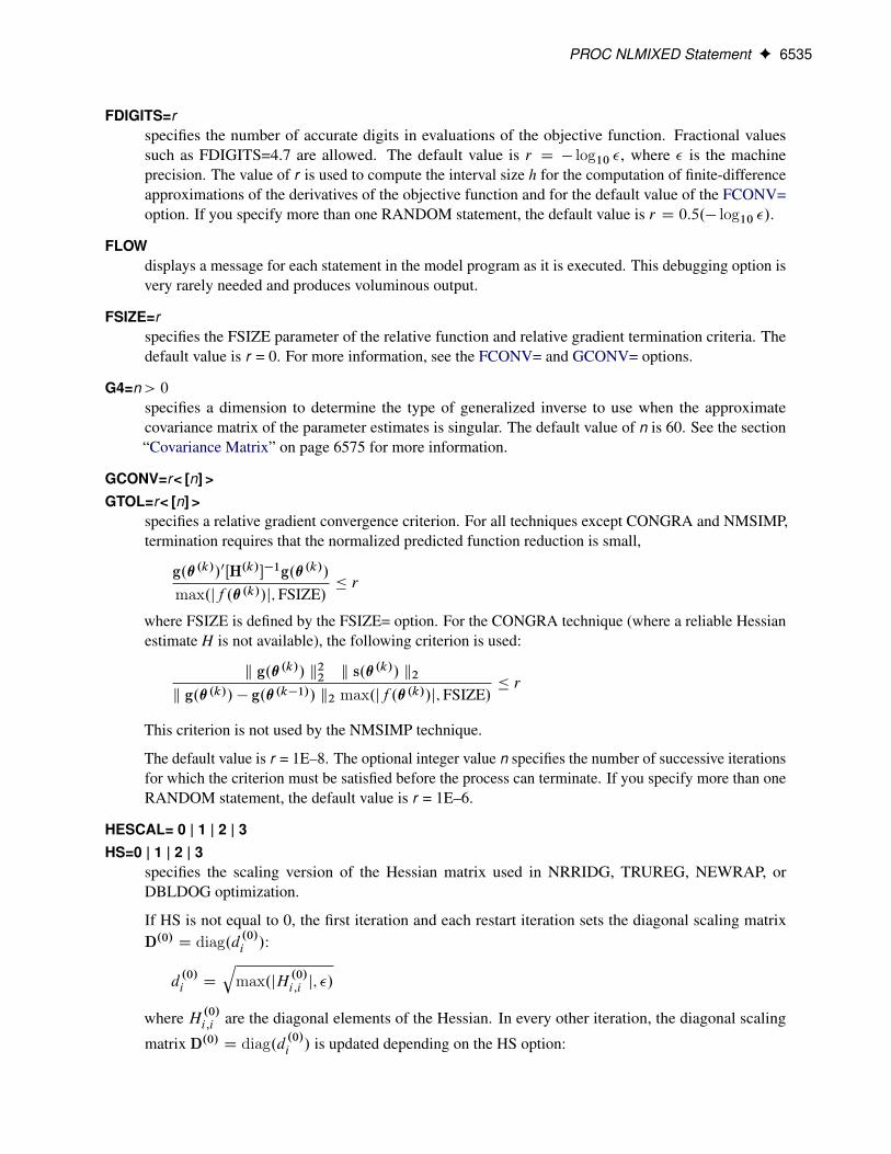
FDIGITS=rspecifies the number of accurate digits in evaluations of the objective function. Fractional valuessuch as FDIGITS=4.7 are allowed. The default value is r D � log10 �, where � is the machineprecision. The value of r is used to compute the interval size h for the computation of finite-differenceapproximations of the derivatives of the objective function and for the default value of the FCONV=option. If you specify more than one RANDOM statement, the default value is r D 0:5.� log10 �/.
FLOWdisplays a message for each statement in the model program as it is executed. This debugging option isvery rarely needed and produces voluminous output.
FSIZE=rspecifies the FSIZE parameter of the relative function and relative gradient termination criteria. Thedefault value is r = 0. For more information, see the FCONV= and GCONV= options.
G4=n> 0specifies a dimension to determine the type of generalized inverse to use when the approximatecovariance matrix of the parameter estimates is singular. The default value of n is 60. See the section“Covariance Matrix” on page 6575 for more information.
GCONV=r< [n] >GTOL=r< [n] >
specifies a relative gradient convergence criterion. For all techniques except CONGRA and NMSIMP,termination requires that the normalized predicted function reduction is small,
g.�.k//0ŒH.k/��1g.�.k//max.jf .�.k//j;FSIZE/
� r
where FSIZE is defined by the FSIZE= option. For the CONGRA technique (where a reliable Hessianestimate H is not available), the following criterion is used:
k g.�.k// k22 k s.�.k// k2k g.�.k// � g.�.k�1// k2 max.jf .�.k//j;FSIZE/
� r
This criterion is not used by the NMSIMP technique.
The default value is r = 1E–8. The optional integer value n specifies the number of successive iterationsfor which the criterion must be satisfied before the process can terminate. If you specify more than oneRANDOM statement, the default value is r = 1E–6.
HESCAL= 0 | 1 | 2 | 3HS=0 | 1 | 2 | 3
specifies the scaling version of the Hessian matrix used in NRRIDG, TRUREG, NEWRAP, orDBLDOG optimization.
If HS is not equal to 0, the first iteration and each restart iteration sets the diagonal scaling matrixD.0/ D diag.d .0/i /:
d.0/i D
qmax.jH .0/
i;i j; �/
where H .0/i;i are the diagonal elements of the Hessian. In every other iteration, the diagonal scaling
matrix D.0/ D diag.d .0/i / is updated depending on the HS option:

6536 F Chapter 82: The NLMIXED Procedure
0 specifies that no scaling is done.
1 specifies the Moré (1978) scaling update:
d.kC1/i D max
�d.k/i ;
qmax.jH .k/
i;i j; �/
�2 specifies the Dennis, Gay, and Welsch (1981) scaling update:
d.kC1/i D max
�0:6 � d
.k/i ;
qmax.jH .k/
i;i j; �/
�3 specifies that di is reset in each iteration:
d.kC1/i D
qmax.jH .k/
i;i j; �/
In each scaling update, � is the relative machine precision. The default value is HS=0. Scaling of theHessian can be time-consuming in the case where general linear constraints are active.
HESSrequests the display of the final Hessian matrix after optimization. If you also specify the STARToption, then the Hessian at the starting values is also printed.
INHESSIAN< =r >INHESS< =r >
specifies how the initial estimate of the approximate Hessian is defined for the quasi-Newton techniquesQUANEW and DBLDOG. There are two alternatives:
� If you do not use the r specification, the initial estimate of the approximate Hessian is set to theHessian at �.0/.� If you do use the r specification, the initial estimate of the approximate Hessian is set to the
multiple of the identity matrix, rI.
By default, if you do not specify the option INHESSIAN=r , the initial estimate of the approximateHessian is set to the multiple of the identity matrix rI, where the scalar r is computed from themagnitude of the initial gradient.
INSTEP=rreduces the length of the first trial step during the line search of the first iterations. For highly nonlinearobjective functions, such as the EXP function, the default initial radius of the trust-region algorithmTRUREG or DBLDOG or the default step length of the line-search algorithms can result in arithmeticoverflows. If this occurs, you should specify decreasing values of 0 < r < 1 such as INSTEP=1E–1,INSTEP=1E–2, INSTEP=1E–4, and so on, until the iteration starts successfully.
� For trust-region algorithms (TRUREG, DBLDOG), the INSTEP= option specifies a factor r > 0for the initial radius �.0/ of the trust region. The default initial trust-region radius is the length ofthe scaled gradient. This step corresponds to the default radius factor of r = 1.� For line-search algorithms (NEWRAP, CONGRA, QUANEW), the INSTEP= option specifies
an upper bound for the initial step length for the line search during the first five iterations. Thedefault initial step length is r = 1.� For the Nelder-Mead simplex algorithm, using TECH=NMSIMP, the INSTEP=r option defines
the size of the start simplex.
For more details, see the section “Computational Problems” on page 6572.

PROC NLMIXED Statement F 6537
ITDETAILSrequests a more complete iteration history, including the current values of the parameter estimates,their gradients, and additional optimization statistics. For further details, see the section “Iterations” onpage 6578.
LCDEACT=r
LCD=rspecifies a threshold r for the Lagrange multiplier that determines whether an active inequalityconstraint remains active or can be deactivated. During minimization, an active inequality constraintcan be deactivated only if its Lagrange multiplier is less than the threshold value r < 0. The defaultvalue is
r D �min.0:01;max.0:1 �ABSGCONV; 0:001 � gmax.k///
where ABSGCONV is the value of the absolute gradient criterion, and gmax.k/ is the maximumabsolute element of the (projected) gradient g.k/ or Z0g.k/. (See the section “Active Set Methods” fora definition of Z.)
LCEPSILON=r > 0
LCEPS=r > 0
LCE=r > 0specifies the range for active and violated boundary constraints. The default value is r = 1E–8. Duringthe optimization process, the introduction of rounding errors can force PROC NLMIXED to increasethe value of r by a factor of 10; 100; : : :. If this happens, it is indicated by a message displayed in thelog.
LCSINGULAR=r > 0
LCSING=r > 0
LCS=r > 0specifies a criterion r , used in the update of the QR decomposition, that determines whether an activeconstraint is linearly dependent on a set of other active constraints. The default value is r = 1E–8. Thelarger r becomes, the more the active constraints are recognized as being linearly dependent. If thevalue of r is larger than 0.1, it is reset to 0.1.
LINESEARCH=i
LIS=ispecifies the line-search method for the CONGRA, QUANEW, and NEWRAP optimization techniques.See Fletcher (1987) for an introduction to line-search techniques. The value of i can be 1; : : : ; 8. ForCONGRA, QUANEW and NEWRAP, the default value is i = 2.
1 specifies a line-search method that needs the same number of function and gradientcalls for cubic interpolation and cubic extrapolation; this method is similar to oneused by the Harwell subroutine library.
2 specifies a line-search method that needs more function than gradient calls forquadratic and cubic interpolation and cubic extrapolation; this method is imple-mented as shown in Fletcher (1987) and can be modified to an exact line search byusing the LSPRECISION= option.

6538 F Chapter 82: The NLMIXED Procedure
3 specifies a line-search method that needs the same number of function and gradientcalls for cubic interpolation and cubic extrapolation; this method is implemented asshown in Fletcher (1987) and can be modified to an exact line search by using theLSPRECISION= option.
4 specifies a line-search method that needs the same number of function and gradientcalls for stepwise extrapolation and cubic interpolation.
5 specifies a line-search method that is a modified version of LIS=4.
6 specifies golden section line search (Polak 1971), which uses only function valuesfor linear approximation.
7 specifies bisection line search (Polak 1971), which uses only function values forlinear approximation.
8 specifies the Armijo line-search technique (Polak 1971), which uses only functionvalues for linear approximation.
LISTdisplays the model program and variable lists. The LIST option is a debugging feature and is notnormally needed.
LISTCODEdisplays the derivative tables and the compiled program code. The LISTCODE option is a debuggingfeature and is not normally needed.
LISTDEPproduces a report that lists, for each variable in the program, the variables that depend on it and onwhich it depends. The LISTDEP option is a debugging feature and is not normally needed.
LISTDERdisplays a table of derivatives. This table lists each nonzero derivative computed for the problem. TheLISTDER option is a debugging feature and is not normally needed.
LOGNOTE< =n >writes periodic notes to the log that describe the current status of computations. It is designed for usewith analyses requiring extensive CPU resources. The optional integer value n specifies the desiredlevel of reporting detail. The default is n = 1. Choosing n = 2 adds information about the objectivefunction values at the end of each iteration. The most detail is obtained with n = 3, which also reportsthe results of function evaluations within iterations.
LSPRECISION=r
LSP=rspecifies the degree of accuracy that should be obtained by the line-search algorithms LIS=2 andLIS=3. Usually an imprecise line search is inexpensive and successful. For more difficult optimizationproblems, a more precise and expensive line search might be necessary (Fletcher 1987). The secondline-search method (which is the default for the NEWRAP, QUANEW, and CONGRA techniques) andthe third line-search method approach exact line search for small LSPRECISION= values. If you havenumerical problems, you should try to decrease the LSPRECISION= value to obtain a more preciseline search. The default values are shown in the following table.
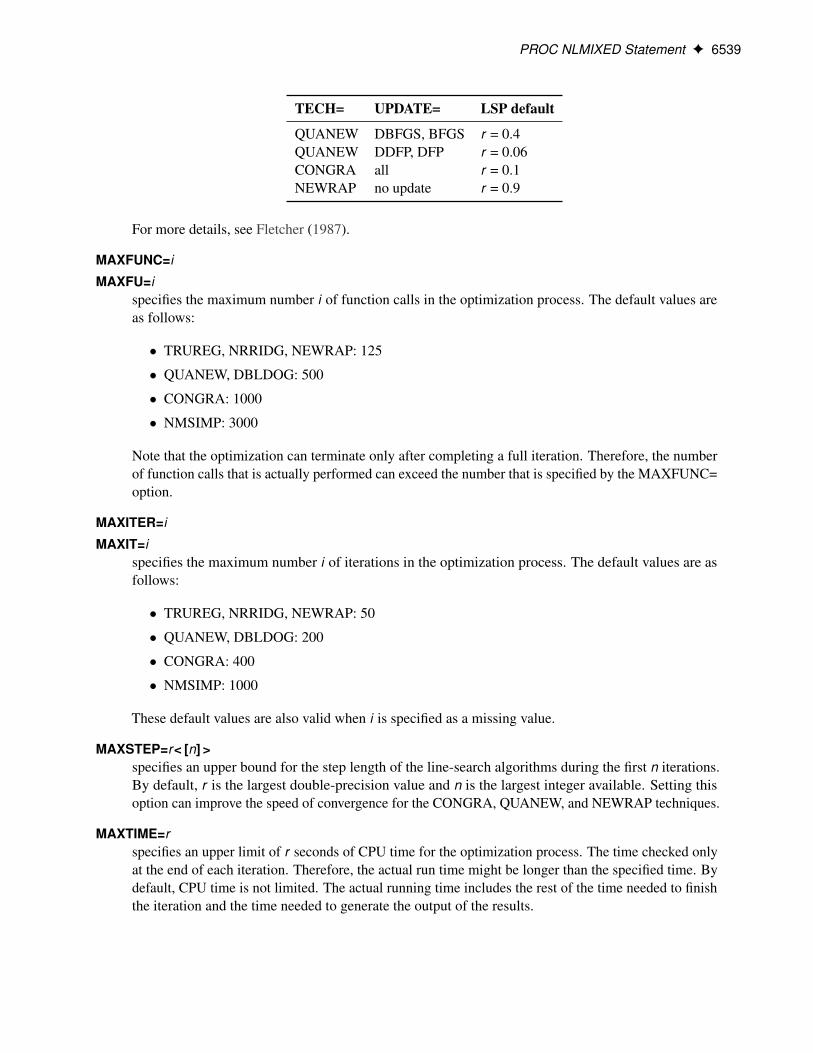
PROC NLMIXED Statement F 6539
TECH= UPDATE= LSP default
QUANEW DBFGS, BFGS r = 0.4QUANEW DDFP, DFP r = 0.06CONGRA all r = 0.1NEWRAP no update r = 0.9
For more details, see Fletcher (1987).
MAXFUNC=i
MAXFU=ispecifies the maximum number i of function calls in the optimization process. The default values areas follows:
� TRUREG, NRRIDG, NEWRAP: 125
� QUANEW, DBLDOG: 500
� CONGRA: 1000
� NMSIMP: 3000
Note that the optimization can terminate only after completing a full iteration. Therefore, the numberof function calls that is actually performed can exceed the number that is specified by the MAXFUNC=option.
MAXITER=i
MAXIT=ispecifies the maximum number i of iterations in the optimization process. The default values are asfollows:
� TRUREG, NRRIDG, NEWRAP: 50
� QUANEW, DBLDOG: 200
� CONGRA: 400
� NMSIMP: 1000
These default values are also valid when i is specified as a missing value.
MAXSTEP=r< [n] >specifies an upper bound for the step length of the line-search algorithms during the first n iterations.By default, r is the largest double-precision value and n is the largest integer available. Setting thisoption can improve the speed of convergence for the CONGRA, QUANEW, and NEWRAP techniques.
MAXTIME=rspecifies an upper limit of r seconds of CPU time for the optimization process. The time checked onlyat the end of each iteration. Therefore, the actual run time might be longer than the specified time. Bydefault, CPU time is not limited. The actual running time includes the rest of the time needed to finishthe iteration and the time needed to generate the output of the results.

6540 F Chapter 82: The NLMIXED Procedure
METHOD=valuespecifies the method for approximating the integral of the likelihood over the random effects. Validvalues are as follows:
FIROspecifies the first-order method of Beal and Sheiner (1982). When using METHOD=FIRO, youmust specify the NORMAL distribution in the MODEL statement and you must also specify aRANDOM statement.
GAUSSspecifies adaptive Gauss-Hermite quadrature (Pinheiro and Bates 1995). You can prevent theadaptation with the NOAD option or prevent adaptive scaling with the NOADSCALE option.This is the default integration method.
HARDYspecifies Hardy quadrature based on an adaptive trapezoidal rule. This method is available onlyfor one-dimensional integrals; that is, you must specify only one random effect.
ISAMPspecifies adaptive importance sampling (Pinheiro and Bates 1995). You can prevent the adaptationwith the NOAD option or prevent adaptive scaling with the NOADSCALE option. You canuse the SEED= option to specify a starting seed for the random number generation used in theimportance sampling. If you do not specify a seed, or if you specify a value less than or equal tozero, the seed is generated from reading the time of day from the computer clock.
MINITER=i
MINIT=ispecifies the minimum number of iterations. The default value is 0. If you request more iterationsthan are actually needed for convergence to a stationary point, the optimization algorithms can behavestrangely. For example, the effect of rounding errors can prevent the algorithm from continuing for therequired number of iterations.
MSINGULAR=r > 0
MSING=r > 0specifies a relative singularity criterion for the computation of the inertia (number of positive, negative,and zero eigenvalues) of the Hessian and its projected forms. The default value is 1E–12 if you do notspecify the SINGHESS= option; otherwise, the default value is max.10�; .1E � 4/ � SINGHESS/.See the section “Covariance Matrix” on page 6575 for more information.
NOADrequests that the Gaussian quadrature be nonadaptive; that is, the quadrature points are centered atzero for each of the random effects and the current random-effects variance matrix is used as the scalematrix.
NOADSCALErequests nonadaptive scaling for adaptive Gaussian quadrature; that is, the quadrature points arecentered at the empirical Bayes estimates for the random effects, but the current random-effectsvariance matrix is used as the scale matrix. By default, the observed Hessian from the current empiricalBayes estimates is used as the scale matrix.

PROC NLMIXED Statement F 6541
NOSORTSUBrequests that the data be processed sequentially and forms a new subject whenever the value of theSUBJECT= variable changes from the previous observation. This option enables PROC NLMIXEDto use the behavior from SAS/STAT 12.3 and previous releases, in which the clusters are constructedby sequential processing. By default, starting with SAS/STAT 13.1, PROC NLMIXED constructs theclusters by using each of the unique SUBJECT= variable values, whether the input data set is sorted ornot.
If you specify more than one RANDOM statement, this option is ignored.
NTHREADS=n> �2specifies the number of threads to use for the log-likelihood calculation that uses the Gaussianquadrature method. When calculating the approximated marginal log likelihood by using the Gaussianquadrature method, PROC NLMIXED allocates data to different threads and calculates the objectivefunction by accumulating values from each thread. NTHREADS=–1 sets the number of availablethreads to the number of hyperthreaded cores available on the system. By default, NTHREADS=1.This option is valid only when METHOD=GAUSS. If you specify more than one RANDOM statement,this option is ignored.
OPTCHECK< =r > 0>computes the function values f .�l/ of a grid of points �l in a ball of radius of r about ��. If youspecify the OPTCHECK option without factor r , the default value is r = 0.1 at the starting point and r= 0.01 at the terminating point. If a point ��
lis found that has a better function value than f .��/, then
optimization is restarted at ��l
.
OUTQ=SAS-data-setspecifies an output data set that contains the quadrature points used for numerical integration.
OUTR=SAS-data-setspecifies an output data set that contains empirical Bayes estimates of the random effects of allhierarchies and their approximate standard errors.
QFAC=r > 0specifies the additive factor used to adaptively search for the number of quadrature points. ForMETHOD=GAUSS, the search sequence is 1, 3, 5, 7, 9, 11, 11 + r , 11 + 2r, . . . , where the defaultvalue of r is 10. For METHOD=ISAMP, the search sequence is 10, 10 + r , 10 + 2r, . . . , where thedefault value of r is 50.
QMAX=r > 0specifies the maximum number of quadrature points permitted before the adaptive search is aborted.The default values are 31 for adaptive Gaussian quadrature, 61 for nonadaptive Gaussian quadrature,160 for adaptive importance sampling, and 310 for nonadaptive importance sampling.
QPOINTS=n> 0specifies the number of quadrature points to be used during evaluation of integrals. ForMETHOD=GAUSS, n equals the number of points used in each dimension of the random effects,resulting in a total of nr points, where r is the number of dimensions. For METHOD=ISAMP, nspecifies the total number of quadrature points regardless of the dimension of the random effects. Bydefault, the number of quadrature points is selected adaptively, and this option disables the adaptivesearch.

6542 F Chapter 82: The NLMIXED Procedure
QSCALEFAC=r > 0specifies a multiplier for the scale matrix used during quadrature calculations. The default value is 1.0.
QTOL=r > 0specifies the tolerance used to adaptively select the number of quadrature points. When the relativedifference between two successive likelihood calculations is less than r , then the search terminates andthe lesser number of quadrature points is used during the subsequent optimization process. The defaultvalue is 1E–4.
RESTART=i > 0
REST=i > 0specifies that the QUANEW or CONGRA algorithm is restarted with a steepest descent/ascent searchdirection after, at most, i iterations. Default values are as follows:
� CONGRA: UPDATE=PB: restart is performed automatically, i is not used.
� CONGRA: UPDATE¤PB: i D min.10n; 80/, where n is the number of parameters.
� QUANEW: i is the largest integer available.
SEED=ispecifies the random number seed for METHOD=ISAMP. If you do not specify a seed, or if youspecify a value less than or equal to zero, the seed is generated from reading the time of day from thecomputer clock. The value must be less than 231 � 1.
SINGCHOL=r > 0specifies the singularity criterion r for Cholesky roots of the random-effects variance matrix and scalematrix for adaptive Gaussian quadrature. The default value is 1E4 times the machine epsilon; thisproduct is approximately 1E–12 on most computers.
SINGHESS=r > 0specifies the singularity criterion r for the inversion of the Hessian matrix. The default value is 1E–8.See the ASINGULAR, MSINGULAR=, and VSINGULAR= options for more information.
SINGSWEEP=r > 0specifies the singularity criterion r for inverting the variance matrix in the first-order method and theempirical Bayes Hessian matrix. The default value is 1E4 times the machine epsilon; this product isapproximately 1E–12 on most computers.
SINGVAR=r > 0specifies the singularity criterion r below which statistical variances are considered to equal zero.The default value is 1E4 times the machine epsilon; this product is approximately 1E–12 on mostcomputers.
STARTrequests that the gradient of the log likelihood at the starting values be displayed. If you also specifythe HESS option, then the starting Hessian is displayed as well.

PROC NLMIXED Statement F 6543
SUBGRADIENT=SAS-data-set
SUBGRAD=SAS-data-setspecifies a SAS data set that contains subgradients. In models that use the RANDOM statement, thedata set contains the subject-specific gradients of the integrated, marginal log likelihood with respectto all parameters. The sum of the subject-specific gradients equals the gradient that is reported in the“Parameter Estimates” table. The data set contains a variable that identifies the subjects.
In models that do not use the RANDOM statement, the data set contains the observation-wise gradient.The variable identifying the SUBJECT= is then replaced with the Observation. This observationcounter includes observations not used in the analysis and is reset in each BY group.
Saving disaggregated gradient information by specifying the SUBGRADIENT= option requires thatyou also specify METHOD=GAUSS or METHOD=ISAMP.
If you specify more than one RANDOM statement, this option is ignored.
TECHNIQUE=value
TECH=valuespecifies the optimization technique. By default, TECH = QUANEW. Valid values are as follows:
� CONGRAperforms a conjugate-gradient optimization, which can be more precisely specified with theUPDATE= option and modified with the LINESEARCH= option. When you specify this option,UPDATE=PB by default.
� DBLDOGperforms a version of double-dogleg optimization, which can be more precisely specified withthe UPDATE= option. When you specify this option, UPDATE=DBFGS by default.
� NMSIMPperforms a Nelder-Mead simplex optimization.
� NONEdoes not perform any optimization. This option can be used as follows:
– to perform a grid search without optimization– to compute estimates and predictions that cannot be obtained efficiently with any of the
optimization techniques
� NEWRAPperforms a Newton-Raphson optimization combining a line-search algorithm with ridging. Theline-search algorithm LIS=2 is the default method.
� NRRIDGperforms a Newton-Raphson optimization with ridging.
� QUANEWperforms a quasi-Newton optimization, which can be defined more precisely with the UPDATE=option and modified with the LINESEARCH= option. This is the default estimation method.
� TRUREGperforms a trust region optimization.

6544 F Chapter 82: The NLMIXED Procedure
TRACEdisplays the result of each operation in each statement in the model program as it is executed. Thisdebugging option is very rarely needed, and it produces voluminous output.
UPDATE=method
UPD=methodspecifies the update method for the quasi-Newton, double-dogleg, or conjugate-gradient optimizationtechnique. Not every update method can be used with each optimizer. See the section “OptimizationAlgorithms” on page 6561 for more information.
Valid methods are as follows:
� BFGSperforms the original Broyden, Fletcher, Goldfarb, and Shanno (BFGS) update of the inverseHessian matrix.
� DBFGSperforms the dual BFGS update of the Cholesky factor of the Hessian matrix. This is the defaultupdate method.
� DDFPperforms the dual Davidon, Fletcher, and Powell (DFP) update of the Cholesky factor of theHessian matrix.
� DFPperforms the original DFP update of the inverse Hessian matrix.
� PBperforms the automatic restart update method of Powell (1977) and Beale (1972).
� FRperforms the Fletcher-Reeves update (Fletcher 1987).
� PRperforms the Polak-Ribiere update (Fletcher 1987).
� CDperforms a conjugate-descent update of Fletcher (1987).
VSINGULAR=r > 0
VSING=r > 0specifies a relative singularity criterion for the computation of the inertia (number of positive, negative,and zero eigenvalues) of the Hessian and its projected forms. The default value is r = 1E–8 if theSINGHESS= option is not specified, and it is the value of SINGHESS= option otherwise. See thesection “Covariance Matrix” on page 6575 for more information.
XCONV=r< [n] >
XTOL=r< [n] >specifies the relative parameter convergence criterion. For all techniques except NMSIMP, terminationrequires a small relative parameter change in subsequent iterations:
maxj j�.k/j � �
.k�1/j j
max.j� .k/j j; j�.k�1/j j;XSIZE/
� r

ARRAY Statement F 6545
For the NMSIMP technique, the same formula is used, but �.k/ is defined as the vertex with the lowestfunction value and �.k�1/ is defined as the vertex with the highest function value in the simplex.
The default value is r = 1E–8 for the NMSIMP technique and r = 0 otherwise. The optional integervalue n specifies the number of successive iterations for which the criterion must be satisfied beforethe process can be terminated.
XREFdisplays a cross-reference of the variables in the program showing where each variable is referencedor given a value. The XREF listing does not include derivative variables. This option is a debuggingfeature and is not normally needed.
XSIZE=r > 0specifies the XSIZE parameter of the relative parameter termination criterion. The default value is r =0. For more details, see the XCONV= option.
ARRAY StatementARRAY arrayname [ dimensions ] < $ > < variables-and-constants > ;
The ARRAY statement is similar to, but not exactly the same as, the ARRAY statement in the SAS DATAstep, and it is exactly the same as the ARRAY statements in the NLIN, NLP, and MODEL procedures. TheARRAY statement is used to associate a name (of no more than eight characters) with a list of variablesand constants. The array name is used with subscripts in the program to refer to the array elements. Thefollowing statements illustrate this:
array r[8] r1-r8;
do i = 1 to 8;r[i] = 0;
end;
The ARRAY statement does not support all the features of the ARRAY statement in the DATA step. It cannotbe used to assign initial values to array elements. Implicit indexing of variables cannot be used; all arrayreferences must have explicit subscript expressions. Only exact array dimensions are allowed; lower-boundspecifications are not supported. A maximum of six dimensions is allowed.
On the other hand, the ARRAY statement does allow both variables and constants to be used as array elements.(Constant array elements cannot have values assigned to them.) Both dimension specification and the list ofelements are optional, but at least one must be specified. When the list of elements is not specified or fewerelements than the size of the array are listed, array variables are created by suffixing element numbers to thearray name to complete the element list.
6546 F Chapter 82: The NLMIXED Procedure
BOUNDS StatementBOUNDS b-con < , b-con . . . > ;
where b-con := number operator parameter_list operator numberor b-con := number operator parameter_listor b-con := parameter_list operator number
and operator := <D, <, >D, or >
Boundary constraints are specified with a BOUNDS statement. One- or two-sided boundary constraints areallowed. The list of boundary constraints are separated by commas. For example:
bounds 0 <= a1-a9 X <= 1, -1 <= c2-c5;bounds b1-b10 y >= 0;
You can specify more than one BOUNDS statement. If you specify more than one lower (upper) bound forthe same parameter, the maximum (minimum) of these is taken.
If the maximum lj of all lower bounds is larger than the minimum of all upper bounds uj for the sameparameter �j , the boundary constraint is replaced by �j WD lj WD min.uj / defined by the minimum of allupper bounds specified for �j .
BY StatementBY variables ;
You can specify a BY statement with PROC NLMIXED to obtain separate analyses of observations in groupsthat are defined by the BY variables. When a BY statement appears, the procedure expects the input dataset to be sorted in order of the BY variables. If you specify more than one BY statement, only the last onespecified is used.
If your input data set is not sorted in ascending order, use one of the following alternatives:
� Sort the data by using the SORT procedure with a similar BY statement.
� Specify the NOTSORTED or DESCENDING option in the BY statement for the NLMIXED procedure.The NOTSORTED option does not mean that the data are unsorted but rather that the data are arrangedin groups (according to values of the BY variables) and that these groups are not necessarily inalphabetical or increasing numeric order.
� Create an index on the BY variables by using the DATASETS procedure (in Base SAS software).
An optimization problem is solved for each BY group separately unless the TECH=NONE option is specified.
For more information about BY-group processing, see the discussion in SAS Language Reference: Concepts.For more information about the DATASETS procedure, see the discussion in the Base SAS Procedures Guide.
CONTRAST Statement F 6547
CONTRAST StatementCONTRAST 'label ' expression < , expression > < options > ;
The CONTRAST statement enables you to conduct a statistical test that several expressions simultaneouslyequal zero. The expressions are typically contrasts—that is, differences whose expected values equal zerounder the hypothesis of interest.
In the CONTRAST statement you must provide a quoted string to identify the contrast and then a list ofvalid SAS expressions separated by commas. Multiple CONTRAST statements are permitted, and resultsfrom all statements are listed in a common table. PROC NLMIXED constructs approximate F tests foreach statement using the delta method (Cox 1998) to approximate the variance-covariance matrix of theconstituent expressions.
The following option is available in the CONTRAST statement:
DF=dspecifies the denominator degrees of freedom to be used in computing p values for the F statistics. Thedefault value corresponds to the DF= option in the PROC NLMIXED statement.
ESTIMATE StatementESTIMATE 'label ' expression < options > ;
The ESTIMATE statement enables you to compute an additional estimate that is a function of the parametervalues. You must provide a quoted string to identify the estimate and then a valid SAS expression. MultipleESTIMATE statements are permitted, and results from all statements are listed in a common table. PROCNLMIXED computes approximate standard errors for the estimates using the delta method (Billingsley 1986).It uses these standard errors to compute corresponding t statistics, p-values, and confidence limits.
The ECOV option in the PROC NLMIXED statement produces a table containing the approximate covariancematrix of all the additional estimates you specify. The ECORR option produces the corresponding correlationmatrix. The EDER option produces a table of the derivatives of the additional estimates with respect to eachof the model parameters.
The following options are available in the ESTIMATE statement:
ALPHA=˛specifies the alpha level to be used in computing confidence limits. The default value corresponds tothe ALPHA= option in the PROC NLMIXED statement.
DF=dspecifies the degrees of freedom to be used in computing p-values and confidence limits. The defaultvalue corresponds to the DF= option in the PROC NLMIXED statement.
ID StatementID names ;
The ID statement identifies additional quantities to be included in the OUT= data set of the PREDICTstatement. These can be any symbols you have defined with SAS programming statements.

6548 F Chapter 82: The NLMIXED Procedure
MODEL StatementMODEL dependent-variable Ï distribution ;
The MODEL statement is the mechanism for specifying the conditional distribution of the data given therandom effects. You must specify a single dependent variable from the input data set, a tilde Ï, and then adistribution with its parameters. Valid distributions are as follows.
� normal(m,v) specifies a normal (Gaussian) distribution with mean m and variance v.
� binary(p) specifies a binary (Bernoulli) distribution with probability p.
� binomial(n,p) specifies a binomial distribution with count n and probability p.
� gamma(a,b) specifies a gamma distribution with shape a and scale b.
� negbin(n,p) specifies a negative binomial distribution with count n and probability p.
� poisson(m) specifies a Poisson distribution with mean m.
� general(ll) specifies a general log likelihood function that you construct using SAS programmingstatements.
The MODEL statement must follow any SAS programming statements you specify for computing parametersof the preceding distributions. See the section “Built-in Log-Likelihood Functions” on page 6557 forexpressions of the built-in conditional log-likelihood functions.
PARMS StatementPARMS < name-list < =numbers > > < , name-list < =numbers > . . . >
< / options > ;
The PARMS statement lists names of parameters and specifies initial values, possibly over a grid. You canspecify the parameters and values directly in a list, or you can provide the name of a SAS data set thatcontains them by using the DATA= option.
While the PARMS statement is not required, you are encouraged to use it to provide PROC NLMIXED withaccurate starting values. Parameters not listed in the PARMS statement are assigned an initial value of 1.PROC NLMIXED considers all symbols not assigned values to be parameters, so you should specify yourmodeling statements carefully and check the output from the “Parameters” table to make sure the properparameters are identified.
A list of parameter names in the PARMS statement is not separated by commas and is followed by an equalsign and a list of numbers. If the number list consists of only one number, this number defines the initialvalue for all the parameters listed to the left of the equal sign.
If the number list consists of more than one number, these numbers specify the grid locations for each of theparameters listed to the left of the equal sign. You can use the TO and BY keywords to specify a number listfor a grid search. If you specify a grid of points in a PARMS statement, PROC NLMIXED computes theobjective function value at each grid point and chooses the best (feasible) grid point as an initial point for the
PREDICT Statement F 6549
optimization process. You can use the BEST= option to save memory for the storing and sorting of all gridpoint information.
The following options are available in the PARMS statement after a slash (/):
BEST=i > 0specifies the maximum number of points displayed in the “Parameters” table, selected as the pointswith the maximum likelihood values. By default, all grid values are displayed.
BYDATAenables you to assign different starting values for each BY group by using the DATA=SAS-data-setoption during BY processing. By default, BY groups are ignored in the PARMS data set. For theBYDATA option to be effective, the DATA= data set must contain the BY variables and the same BYgroups as the primary input data set. When you supply a grid of starting values with the DATA= dataset and the BYDATA option is in effect, the size of the grid is determined by the first BY group.
DATA=SAS-data-setspecifies a SAS data set containing parameter names and starting values. The data set should be inone of two forms: narrow or wide. The narrow-form data set contains the variables Parameter andEstimate, with parameters and values listed as distinct observations. The wide-form data set has theparameters themselves as variables, and each observation provides a different set of starting values.By default, BY groups are ignored in this data set, so the same starting grid is evaluated for each BYgroup. You can vary the starting values for BY groups by using the BYDATA option.
PREDICT StatementPREDICT expression OUT=SAS-data-set < options > ;
The PREDICT statement enables you to construct predictions of an expression across all of the observations inthe input data set. Any valid SAS programming expression involving the input data set variables, parameters,and random effects is valid. Predicted values are computed using the parameter estimates and empiricalBayes estimates of the random effects. Standard errors of prediction are computed using the delta method(Billingsley 1986; Cox 1998). Results are placed in an output data set that you specify with the OUT=option. Besides all variables from the input data set, the OUT= data set contains the following variables:Pred, StdErrPred, DF, tValue, Probt, Alpha, Lower, Upper. You can also add other computed quantities tothis data set with the ID statement.
The following options are available in the PREDICT statement:
ALPHA=˛specifies the alpha level to be used in computing t statistics and intervals. The default value correspondsto the ALPHA= option in the PROC NLMIXED statement.
DERrequests that derivatives of the predicted expression with respect to all parameters be included in theOUT= data set. The variable names for the derivatives are the same as the parameter names with theprefix “Der_” appended. All of the derivatives are evaluated at the final estimates of the parametersand the empirical Bayes estimates of the random effects.
DF=dspecifies the degrees of freedom to be used in computing t statistics and intervals in the OUT= data set.The default value corresponds to the DF= option in the PROC NLMIXED statement.

6550 F Chapter 82: The NLMIXED Procedure
RANDOM StatementRANDOM random-effects Ï distribution SUBJECT=variable < options > ;
The RANDOM statement defines the random effects and their distribution. The random effects must berepresented by symbols that appear in your SAS programming statements. The random effects usuallyinfluence the mean value of the distribution that is specified in the MODEL statement. The RANDOMstatement consists of a list of the random effects (usually just one or two symbols), a tilde (Ï), the distributionof the random effects, and then a SUBJECT= variable.
The only distribution available for the random effects is normal(m,v), with mean m and variance v.
This syntax is illustrated as follows for one effect:
random u ~ normal(0,s2u) subject=clinic;
For multiple effects, you should specify bracketed vectors for m and v, the latter consisting of the lowertriangle of the random-effects variance matrix listed in row order. This is illustrated for two random effectsas follows:
random b1 b2 ~ normal([0,0],[g11,g21,g22]) subject=person;
Similarly, the syntax for three random effects is illustrated as follows:
random b1 b2 b3 ~ normal([0,0,0],[g11,g21,g22,g31,g32,g33])subject=person;
The SUBJECT= variable determines the unique realizations of the random effects.
PROC NLMIXED constructs the subject clusters based on unique values in the SUBJECT= variable. Thisconstruction process of clusters, starting in SAS/STAT 13.1, is different from that in earlier releases of PROCNLMIXED, where a change in the SUBJECT= variable value indicates a new cluster. Because of this change,starting in SAS/STAT 13.1, the input data set does not need to be sorted by SUBJECT= variable to use theunique SUBJECT= variable values.
On the other hand, in earlier releases of SAS/STAT, PROC NLMIXED does not sort the input data set foryou; rather, it processes the data sequentially and considers an observation to be from a new subject wheneverthe value of its SUBJECT= variable changes from the previous observation. To revert to this sequentialprocess behavior of SAS/STAT 12.3 and previous releases, specify the NOSORTSUB option in the PROCNLMIXED statement.
You can specify multiple RANDOM statements; this is supported starting in SAS/STAT 13.2. When youspecify more than one RANDOM statement, PROC NLMIXED assumes that the SUBJECT= variablefrom each RANDOM statement forms a containment hierarchy. For more information, see the section“Hierarchical Model Specification” on page 6559. The syntax for two RANDOM statements is illustrated asfollows:
random r11 ~ normal(0,sd1) subject = school;random r21 ~ normal(0,sd2) subject = class(school);
You can specify the following options in the RANDOM statement:

REPLICATE Statement F 6551
ALPHA=˛specifies the alpha level to be used in computing t statistics and intervals. The default value correspondsto the value of the ALPHA= option in the PROC NLMIXED statement.
DF=dspecifies the degrees of freedom to be used in computing t statistics and intervals in the OUT= data set.PROC NLMIXED calculates the default degrees of freedom as follows:
� When only one or no RANDOM statement is specified, the default value corresponds to the valueof the DF= option in the PROC NLMIXED statement.
� When multiple RANDOM statements are specified, the default value is the number of subjectsminus the number of random-effects variables in the corresponding RANDOM statement.
OUT=SAS-data-setrequests an output data set that contains empirical Bayes estimates of the random effects and theirapproximate standard errors of prediction.
REPLICATE StatementREPLICATE variable ;
The REPLICATE statement provides a way to accommodate models in which different subjects have identicaldata. This occurs most commonly when the dependent variable is binary. When you specify a REPLICATEvariable, PROC NLMIXED treats its value as the number of subjects that have data identical to the data forthe current value of the SUBJECT= variable (specified in the RANDOM statement). Only the last observationof the REPLICATE variable for each subject is used, and the replicate variable must have only positivevalues.
The function of a REPLICATE statement is related to but not quite the same as the function of either a FREQor a WEIGHT statement in other statistical modeling procedures, such as the GLM, GENMOD, GLIMMIX,and LOGISTIC procedures. A FREQ or a WEIGHT value essentially multiplies the log likelihood or sumof squares contribution for each observation. On the other hand, a REPLICATE value multiplies the loglikelihood contribution of each subject, which consists of one or more observations. When no SUBJECT=variable is specified, the REPLICATE value behaves like a weight, multiplying each observation’s loglikelihood contribution.
NOTE: The REPLICATE statement is not allowed when there is more than one RANDOM statement.
Programming StatementsThis section lists the programming statements that are used to code the log-likelihood function in PROCNLMIXED. It also documents the differences between programming statements in PROC NLMIXED andprogramming statements in the SAS DATA step. The syntax of programming statements used in PROCNLMIXED is identical to that used in the CALIS and GENMOD procedures (see Chapter 29 and Chapter 44,respectively), and the MODEL procedure (see the SAS/ETS User’s Guide). Most of the programmingstatements that can be used in the SAS DATA step can also be used in the NLMIXED procedure. See SASLanguage Reference: Dictionary for a description of SAS programming statements. The following are validstatements:

6552 F Chapter 82: The NLMIXED Procedure
ABORT;ARRAY arrayname < [ dimensions ] > < $ > < variables-and-constants >;CALL name < (expression < , expression . . . >) >;DELETE;DO < variable = expression < TO expression > < BY expression > >
< , expression < TO expression > < BY expression > > . . .< WHILE expression > < UNTIL expression >;
END;GOTO statement-label;IF expression;IF expression THEN program-statement;
ELSE program-statement;variable = expression;variable + expression;LINK statement-label;PUT < variable > < = > . . . ;RETURN;SELECT < (expression) >;STOP;SUBSTR(variable, index , length)= expression;WHEN (expression)program-statement;
OTHERWISE program-statement;
For the most part, the SAS programming statements work the same as they do in the SAS DATA step, asdocumented in SAS Language Reference: Concepts; however, there are the following differences:
� The ABORT statement does not allow any arguments.
� The DO statement does not allow a character index variable. Thus
do i = 1,2,3;
is supported, but the following statement is not supported:
do i = 'A','B','C';
� The LAG function does work appropriately with PROC NLMIXED, but you can use the ZLAGfunction instead.
� The PUT statement, used mostly for program debugging in PROC NLMIXED, supports only some ofthe features of the DATA step PUT statement, and it has some new features that the DATA step PUTstatement does not.
– The PROC NLMIXED PUT statement does not support line pointers, factored lists, iterationfactors, overprinting, _INFILE_, the colon (:) format modifier, or “$”.
– The PROC NLMIXED PUT statement does support expressions, but the expression must beenclosed in parentheses. For example, the following statement displays the square root of x:put .sqrt.x//I

Details: NLMIXED Procedure F 6553
– The PROC NLMIXED PUT statement supports the item _PDV_ to display a formatted listing ofall variables in the program. For example, the following statement displays a much more readablelisting of the variables than the _ALL_ print item:put _pdv_I
� The WHEN and OTHERWISE statements enable you to specify more than one target statement. Thatis, DO/END groups are not necessary for multiple statement WHENs. For example, the followingsyntax is valid:
select;when (exp1) stmt1;
stmt2;when (exp2) stmt3;
stmt4;end;
When coding your programming statements, you should avoid defining variables that begin with an underscore(_), because they might conflict with internal variables created by PROC NLMIXED. The MODEL statementmust come after any SAS programming statements that define or modify terms used in the construction ofthe log-likelihood.
Details: NLMIXED ProcedureThis section contains details about the underlying theory and computations of PROC NLMIXED.
Modeling Assumptions and NotationPROC NLMIXED operates under the following general framework for nonlinear mixed models. Assumethat you have an observed data vector yi for each of i subjects, i D 1; : : : ; s. The yi are assumed to beindependent across i, but within-subject covariance is likely to exist because each of the elements of yiis measured on the same subject. As a statistical mechanism for modeling this within-subject covariance,assume that there exist latent random-effect vectors ui of small dimension (typically one or two) that are alsoindependent across i. Assume also that an appropriate model linking yi and ui exists, leading to the jointprobability density function
p.yi jXi ;�; ui /q.ui j�/
where Xi is a matrix of observed explanatory variables and � and � are vectors of unknown parameters.
Let � D Œ�; �� and assume that it is of dimension n. Then inferences about � are based on the marginallikelihood function
m.�/ D
sYiD1
Zp.yi jXi ;�; ui /q.ui j�/dui

6554 F Chapter 82: The NLMIXED Procedure
In particular, the function
f .�/ D � logm.�/
is minimized over � numerically in order to estimate � , and the inverse Hessian (second derivative) matrix atthe estimates provides an approximate variance-covariance matrix for the estimate of � . The function f .�/is referred to both as the negative log likelihood function and as the objective function for optimization.
As an example of the preceding general framework, consider the nonlinear growth curve example in the section“Getting Started: NLMIXED Procedure” on page 6520. Here, the conditional distribution p.yi jXi ;�; ui / isnormal with mean
b1 C ui1
1C expŒ�.dij � b2/=b3�
and variance �2e ; thus � D Œb1; b2; b3; �2e �. Also, ui is a scalar and q.ui j�/ is normal with mean 0 and
variance �2u ; thus � D �2u .
The following additional notation is also found in this chapter. The quantity �.k/ refers to the parametervector at the kth iteration, the vector g.�/ refers to the gradient vector rf .�/, and the matrix H.�/ refers tothe Hessian r2f .�/. Other symbols are used to denote various constants or option values.
Nested Multilevel Nonlinear Mixed Models
The general framework for nested multilevel nonlinear mixed models in cases of two levels can be explainedas follows. Let yj.i/ be the response vector observed on subject j that is nested within subject i, wherej is commonly referred as the second-level subject and i is the first-level subject. There are s first-levelsubjects, and each has si second-level subjects that are nested within. An example is yj.i/, which are theheights of students in class j of school i, where j D 1; : : : ; si for each i and i D 1; : : : ; s. Suppose thereexist latent random-effect vectors vj.i/ and vi of small dimensions for modeling within subject covariance.Assume also that an appropriate model that links yj.i/ and .vj.i/; vi / exists, and if you use the notationyi D .y1.i/; : : : ; ysi .i//, ui D .vi ; v1.i/; : : : ; vsi .i//, and � D .�1; �2/, the joint density function in terms ofthe first-level subject can be expressed as
p.yi jXi ;�; ui /q.ui j�/ D
0@ siYjD1
p.yj.i/jXi ;�; vi ; vj.i//q2.vj.i/j�2/
1A q1.vi j�1/As defined in the previous section, the marginal likelihood function where � D Œ�; �� is
m.�/ D
sYiD1
Zp.yi jXi ;�; ui /q.ui j�/dui
Again, the function
f .�/ D � logm.�/
is minimized over � numerically in order to estimate � . Models that have more than two levels follow similarnotation.

Integral Approximations F 6555
Integral ApproximationsAn important part of the marginal maximum likelihood method described previously is the computation ofthe integral over the random effects. The default method in PROC NLMIXED for computing this integral isadaptive Gaussian quadrature as described in Pinheiro and Bates (1995). Another approximation method isthe first-order method of Beal and Sheiner (1982, 1988). A description of these two methods follows.
Adaptive Gaussian Quadrature
A quadrature method approximates a given integral by a weighted sum over predefined abscissas for therandom effects. A good approximation can usually be obtained with an adequate number of quadrature pointsas well as appropriate centering and scaling of the abscissas. Adaptive Gaussian quadrature for the integralover ui centers the integral at the empirical Bayes estimate of ui , defined as the vectorbui that minimizes
� log Œp.yi jXi ;�; ui /q.ui j�/�
with � and � set equal to their current estimates. The final Hessian matrix from this optimization can be usedto scale the quadrature abscissas.
Suppose .zj ; wj I j D 1; : : : ; p/ denote the standard Gauss-Hermite abscissas and weights (Golub andWelsch 1969, or Table 25.10 of Abramowitz and Stegun 1972). The adaptive Gaussian quadrature integralapproximation is as follows:Z
p.yi jXi ;�; ui /q.ui j�/dui �
2r=2 j�.Xi ;�/j�1=2pX
j1D1
� � �
pXjrD1
"p.yi jXi ;�; aj1;:::;jr /q.aj1;:::;jr j�/
rYkD1
wjk exp z2jk
#
where r is the dimension of ui , �.Xi ;�/ is the Hessian matrix from the empirical Bayes minimization,zj1;:::;jr is a vector with elements .zj1 ; : : : ; zjr /, and
aj1;:::;jr Dbui C 21=2�.Xi ;�/�1=2zj1;:::;jrPROC NLMIXED selects the number of quadrature points adaptively by evaluating the log-likelihoodfunction at the starting values of the parameters until two successive evaluations have a relative differenceless than the value of the QTOL= option. The specific search sequence is described under the QFAC= option.Using the QPOINTS= option, you can adjust the number of quadrature points p to obtain different levelsof accuracy. Setting p = 1 results in the Laplacian approximation as described in: Beal and Sheiner (1992);Wolfinger (1993); Vonesh (1992, 1996); Vonesh and Chinchilli (1997); Wolfinger and Lin (1997).
The NOAD option in the PROC NLMIXED statement requests nonadaptive Gaussian quadrature. Here allbui are set equal to zero, and the Cholesky root of the estimated variance matrix of the random effects issubstituted for �.Xi ;�/�1=2 in the preceding expression for aj1;:::;jr . In this case derivatives are computedusing the algorithm of Smith (1995). The NOADSCALE option requests the same scaling substitutionbut with the empirical Bayes bui . When there is one RANDOM statement, the dimension of ui is thenumber of random effects that are specified in that RANDOM statement. For nested multilevel nonlinearmixed models, the dimension of ui could increase significantly. In this case, the dimension of ui isequal to the sum of all nested subjects times the corresponding random-effects dimension. For example,

6556 F Chapter 82: The NLMIXED Procedure
consider a three-level nested nonlinear mixed model that contains s first-level subjects, where each first-level subject has si second-level subjects that are nested within and sij third-level subjects that are nestedwithin each combination of first-level subject i and second-level subject j. Then, based on notation inthe previous section, ui D .vi ; v1.i/; v1.i1/; : : : ; vsi1.i1/; : : : ; vsi .i/; v1.isi /; : : : ; vsisi .isi //. Suppose ri isthe random-effects dimension at level i. Then the dimension of ui , denoted as r, can be computed asr D r1 C .r2 � si /C
�r3 �
PsijD1 sij
�. Hence the joint estimation of ui is more costly.
When only one RANDOM statement is specified for the model, by default PROC NLMIXED uses Newton-Raphson optimization for empirical Bayes minimization of random effects for each subject. If you specifythe EBOPT option in the PROC NLMIXED statement, then the procedure uses Newton-Raphson ridgeoptimization. But when multiple RANDOM statements are specified, quasi-Newton optimization is usedfor the empirical Bayes minimization of random effects for each subject. Therefore, all the options thatare related to the Newton-Raphson method (such as the EBOPT, EBSSFRAC=, EBSSTOL=, EBSTEPS=,EBSUBSTEPS=, and EBTOL= options) are ignored.
PROC NLMIXED computes the derivatives of the adaptive Gaussian quadrature approximation whencarrying out the default dual quasi-Newton optimization. For nested multilevel nonlinear mixed models,PROC NLMIXED does not explicitly compute these derivatives. In this case, it ignores the EMPIRICALand SUBGRADIENT= options in the PROC NLMIXED statement. Also, nested multilevel nonlinear mixedmodels use METHOD=GAUSS only. In addition to these changes, for nested multilevel nonlinear mixedmodels, the default values of GTOL and ABSGTOL are changed to 1E–6 and 1E–3, respectively.
First-Order Method
Another integral approximation available in PROC NLMIXED is the first-order method of Beal and Sheiner(1982, 1988) and Sheiner and Beal (1985). This approximation is used only in the case where p.yi jXi ;�; ui /is normal—that is,
p.yi jXi ;�; ui / D .2�/�ni=2 jRi .Xi ;�/j�1=2
exp˚�.1=2/ Œyi �mi .Xi ;�; ui /�0Ri .Xi ;�/�1 Œyi �mi .Xi ;�; ui /�
where ni is the dimension of yi , Ri is a diagonal variance matrix, and mi is the conditional mean vector ofyi .
The first-order approximation is obtained by expanding mi .Xi ;�; ui /with a one-term Taylor series expansionabout ui D 0, resulting in the approximation
p.yi jXi ;�; ui / � .2�/�ni=2 jRi .Xi ;�/j�1=2
exp��.1=2/ Œyi �mi .Xi ;�; 0/ � Zi .Xi ;�/ui �0
Ri .Xi ;�/�1 Œyi �mi .Xi ;�; 0/ � Zi .Xi ;�/ui ��
where Zi .Xi ;�/ is the Jacobian matrix @mi .Xi ;�; ui /=@ui evaluated at ui D 0.
Assuming that q.ui j�/ is normal with mean 0 and variance matrix G.�/, the first-order integral approximationis computable in closed form after completing the square:Z
p.yi jXi ;�; ui /q.ui j�/ dui � .2�/�ni=2 jVi .Xi ;�/j�1=2
exp��.1=2/ Œyi �mi .Xi ;�; 0/�0Vi .Xi ;�/�1 Œyi �mi .Xi ;�; 0/�
�

Built-in Log-Likelihood Functions F 6557
where Vi .Xi ;�/ D Zi .Xi ;�/G.�/Zi .Xi ;�/0 C Ri .Xi ;�/. The resulting approximation for f .�/ is thenminimized over � D Œ�; �� to obtain the first-order estimates. PROC NLMIXED uses finite-differencederivatives of the first-order integral approximation when carrying out the default dual quasi-Newtonoptimization.
Built-in Log-Likelihood FunctionsThis section displays the basic formulas used by the NLMIXED procedure to compute the conditionallog-likelihood functions of the data given the random effects. Note, however, that in addition to these basicequations, the NLMIXED procedure employs a number of checks for missing values and floating-pointarithmetic. You can see the entire program used by the NLMIXED procedure to compute the conditionallog-likelihood functions l.�Iy/ by adding the LIST debugging option to the PROC NLMIXED statement.
Y � normal.m; v/
l.m; vIy/ D �1
2
�logf2�g C
.y �m/2
vC logfvg
�EŒY � D m
VarŒY � D vv > 0
Y � binary.p/
l1.pIy/ D
�y logfpg y > 0
0 otherwise
l2.pIy/ D
�.1 � y/ logf1 � pg y < 1
0 otherwise
l.pIy/ D l1.pIy/C l2.pIy/
EŒY � D pVarŒY � D p .1 � p/
0 < p < 1
Y � binomial.n; p/
lc D logf�.nC 1/g � logf�.y C 1/g � logf�.n � y C 1/g
l1.n; pIy/ D
�y logfpg y > 0
0 otherwise
l2.n; pIy/ D
�.n � y/ logf1 � pg n � y > 0
0 otherwise
l.n; pIy/ D lc C l1.n; pIy/C l2.n; pIy/
EŒY � D npVarŒY � D np .1 � p/
0 < p < 1

6558 F Chapter 82: The NLMIXED Procedure
Y � gamma.a; b/
l.a; bIy/ D �a logfbg � logf�.a/g C .a � 1/ logfyg � y=bEŒY � D ab
VarŒY � D ab2
a > 0
b > 0
This parameterization of the gamma distribution differs from the parameterization used inthe GLIMMIX and GENMOD procedures. The following statements show the equivalentreparameterization in the NLMIXED procedure that fits a generalized linear model forgamma-distributed data in the parameterization of the GLIMMIX procedure:
proc glimmix;model y = x / dist=gamma s;
run;
proc nlmixed;parms b0=1 b1=0 scale=14;linp = b0 + b1*x;mu = exp(linp);b = mu/scale;model y ~ gamma(scale,b);
run;
Y � negbin.n; p/
l.n; pIy/ D logf�.nC y/g � logf�.n/g � logf�.y C 1/gC n logfpg C y logf1 � pg
EŒY � D nP D n�1 � p
p
�VarŒY � D nP.1 � P / D n
�1 � p
p
�1
p
n � 0
0 < p < 1
This form of the negative binomial distribution is one of the many parameterizations inwhich the mass function or log-likelihood function appears. Another common parameteri-zation uses
l.n; pIy/ D logf�.nC y/g � logf�.n/g � logf�.y C 1/gC n logf1 � P=.1C P /g C y logfP=.1C P /g
with P D .1 � p/=p, P > 0.
Note that the parameter n can be real-numbered; it does not have to be integer-valued.The parameterization of the negative binomial distribution in the NLMIXED procedurediffers from that in the GLIMMIX and GENMOD procedures. The following statementsshow the equivalent formulations for maximum likelihood estimation in the GLIMMIXand NLMIXED procedures in a negative binomial regression model:

Hierarchical Model Specification F 6559
proc glimmix;model y = x / dist=negbin s;
run;
proc nlmixed;parms b0=3, b1=1, k=0.8;linp = b0 + b1*x;mu = exp(linp);p = 1/(1+mu*k);model y ~ negbin(1/k,p);
run;
Y � Poisson.m/
l.mIy/ D y logfmg �m � logf�.y C 1/gEŒY � D m
VarŒY � D mm > 0
Hierarchical Model SpecificationPROC NLMIXED supports multiple RANDOM statements to accommodate nested multilevel nonlinearmixed models, starting with SAS/STAT 13.2. If you use multiple RANDOM statements, PROC NLMIXEDassumes that the SUBJECT= variable from each RANDOM statement forms a containment hierarchy. Inthe containment hierarchy, each SUBJECT= variable is contained by another SUBJECT= variable, and theSUBJECT= variable that is contained by all SUBJECT= variables is considered “the” SUBJECT= variable.For example, consider the following three-level nested model that has three SUBJECT= variables:
A B C
1 1 11 1 21 2 11 2 22 1 12 1 22 1 32 2 12 2 2
Suppose you specify a three-level nested model by using the following three RANDOM statements:

6560 F Chapter 82: The NLMIXED Procedure
random r11 ~ normal(0,sd1) subject = A;random r21 ~ normal(0,sd2) subject = B(A);random r31 ~ normal(0,sd3) subject = C(A*B);
Then PROC NLMIXED assumes the containment hierarchy as follows. The first-level hierarchy is definedusing “the” SUBJECT= variable A. Similarly, the second-level hierarchy is defined using SUBJECT= variableB, which is nested within first level. Finally, SUBJECT= variable C defines the third-level hierarchy thatis nested within both the first and second levels. In short, the SUBJECT= variable A is “the” SUBJECT=variable. B is contained in A, and C is contained in both A and B. In this example, there are two first-levelsubjects that are determined using “the” SUBJECT= variable A.
Based on the preceding hierarchy specification, PROC NLMIXED’s indexing of nested subjects for eachfirst-level subject can be visualized as follows:
A1‚ …„ ƒB1.1/‚ …„ ƒ
C1.11/C2.11/
B2.1/‚ …„ ƒC1.12/C2.12/
A2‚ …„ ƒB1.2/‚ …„ ƒ
C1.21/C2.21/C3.21/
B2.2/‚ …„ ƒC1.22/C2.22/
The ith subject from the first level is denoted as Ai , the second-level nested subjects are denoted as Bj.i/, andthe third-level nested subjects are denoted as Ck.ij /.
You can specify any nested structure by using the SUBJECT= syntax in PROC NLMIXED. For example,using the following three RANDOM statements, PROC NLMIXED fits a different model:
random r11 ~ normal(0,sd1) subject = C;random r21 ~ normal(0,sd2) subject = B(C);random r31 ~ normal(0,sd3) subject = A(C*B);
In this case, PROC NLMIXED processes the subjects by using SUBJECT= variable C as “the” SUBJECT=variable, and the containment hierarchy is changed as follows:
A B C
1 1 11 1 21 2 11 2 22 1 12 1 22 1 32 2 12 2 2
)
C B A
1 1 11 1 21 2 11 2 22 1 12 1 22 2 12 2 23 1 2
Again, PROC NLMIXED’s indexing of the nested subjects in this containment hierarchy can be visualized asfollows:
C1‚ …„ ƒB1.1/‚ …„ ƒ
A1.11/A2.11/
B2.1/‚ …„ ƒA1.12/A2.12/
C2‚ …„ ƒB1.2/‚ …„ ƒ
A1.21/A2.21/
B2.2/‚ …„ ƒA1.22/A2.22/
C3‚…„ƒB1.3/‚…„ƒA1.31/

Optimization Algorithms F 6561
Here, PROC NLMIXED assumes that C is “the” SUBJECT= variable. B is contained in C, and A is containedin C and B. In this case, there are three first-level subjects that are determined using “the” SUBJECT=variable C.
As explained before, in this case, the ith subject from the first level is denoted as Ci , the second-level nestedsubjects are denoted as Bj.i/ and for third level, the nested subjects are denoted as Ak.ij /.
Note that the containment hierarchy could potentially create more subjects than the unique number of subjects.For example, consider the following table, in which A is “the” SUBJECT= variable and B is nested withinthe subject A:
A B
a 1a 2b 1b 2c 1c 2
Even though the SUBJECT = B variable has only two unique subjects (1 and 2), when the containmenthierarchy that is specified along with B is nested within A, PROC NLMIXED creates six nested B subjects.These nested subjects can be denoted as 1(a), 2(a), 1(b), 2(b), 1(c), and 2(c).
PROC NLMIXED does not support noncontainment hierarchy (or non-nested) models. For example, thefollowing statements are not supported, because subject C is not nested within B and A:
random r11 ~ normal(0,sd1) subject = A;random r21 ~ normal(0,sd2) subject = B(A);random r31 ~ normal(0,sd3) subject = C;
Optimization AlgorithmsThere are several optimization techniques available in PROC NLMIXED. You can choose a particularoptimizer with the TECH= option in the PROC NLMIXED statement.
Algorithm TECH=
trust region method TRUREGNewton-Raphson method with line search NEWRAPNewton-Raphson method with ridging NRRIDGquasi-Newton methods (DBFGS, DDFP, BFGS, DFP) QUANEWdouble-dogleg method (DBFGS, DDFP) DBLDOGconjugate gradient methods (PB, FR, PR, CD) CONGRANelder-Mead simplex method NMSIMP
No algorithm for optimizing general nonlinear functions exists that always finds the global optimum fora general nonlinear minimization problem in a reasonable amount of time. Since no single optimization

6562 F Chapter 82: The NLMIXED Procedure
technique is invariably superior to others, PROC NLMIXED provides a variety of optimization techniquesthat work well in various circumstances. However, you can devise problems for which none of the techniquesin PROC NLMIXED can find the correct solution. Moreover, nonlinear optimization can be computationallyexpensive in terms of time and memory, so you must be careful when matching an algorithm to a problem.
All optimization techniques in PROC NLMIXED use O.n2/ memory except the conjugate gradient methods,which use only O.n/ of memory and are designed to optimize problems with many parameters. Since thetechniques are iterative, they require the repeated computation of the following:
� the function value (optimization criterion)
� the gradient vector (first-order partial derivatives)
� for some techniques, the (approximate) Hessian matrix (second-order partial derivatives)
However, since each of the optimizers requires different derivatives, some computational efficiencies can begained. The following table shows, for each optimization technique, which derivatives are required (FOD:first-order derivatives; SOD: second-order derivatives).
Algorithm FOD SOD
TRUREG x xNEWRAP x xNRRIDG x x
QUANEW x -DBLDOG x -CONGRA x -NMSIMP - -
Each optimization method employs one or more convergence criteria that determine when it has converged.The various termination criteria are listed and described in the “PROC NLMIXED Statement” section.An algorithm is considered to have converged when any one of the convergence criteria is satisfied. Forexample, under the default settings, the QUANEW algorithm will converge if ABSGCONV< 1E–5, FCONV<10�FDIGITS, or GCONV< 1E–8.
Choosing an Optimization Algorithm
The factors that go into choosing a particular optimization technique for a particular problem are complexand can involve trial and error.
For many optimization problems, computing the gradient takes more computer time than computing thefunction value, and computing the Hessian sometimes takes much more computer time and memory thancomputing the gradient, especially when there are many decision variables. Unfortunately, optimizationtechniques that do not use some kind of Hessian approximation usually require many more iterations thantechniques that do use a Hessian matrix, and as a result the total run time of these techniques is often longer.Techniques that do not use the Hessian also tend to be less reliable. For example, they can more easilyterminate at stationary points rather than at global optima.
A few general remarks about the various optimization techniques follow:

Optimization Algorithms F 6563
� The second-derivative methods TRUREG, NEWRAP, and NRRIDG are best for small problems wherethe Hessian matrix is not expensive to compute. Sometimes the NRRIDG algorithm can be faster thanthe TRUREG algorithm, but TRUREG can be more stable. The NRRIDG algorithm requires only onematrix with n.nC 1/=2 double words; TRUREG and NEWRAP require two such matrices.
� The first-derivative methods QUANEW and DBLDOG are best for medium-sized problems where theobjective function and the gradient are much faster to evaluate than the Hessian. The QUANEW andDBLDOG algorithms, in general, require more iterations than TRUREG, NRRIDG, and NEWRAP, buteach iteration can be much faster. The QUANEW and DBLDOG algorithms require only the gradientto update an approximate Hessian, and they require slightly less memory than TRUREG or NEWRAP(essentially one matrix with n.nC 1/=2 double words). QUANEW is the default optimization method.
� The first-derivative method CONGRA is best for large problems where the objective function andthe gradient can be computed much faster than the Hessian and where too much memory is requiredto store the (approximate) Hessian. The CONGRA algorithm, in general, requires more iterationsthan QUANEW or DBLDOG, but each iteration can be much faster. Since CONGRA requires only afactor of n double-word memory, many large applications of PROC NLMIXED can be solved only byCONGRA.
� The no-derivative method NMSIMP is best for small problems where derivatives are not continuous orare very difficult to compute.
Algorithm Descriptions
Some details about the optimization techniques follow.
Trust Region Optimization (TRUREG)The trust region method uses the gradient g.�.k// and the Hessian matrix H.�.k//; thus, it requires that theobjective function f .�/ have continuous first- and second-order derivatives inside the feasible region.
The trust region method iteratively optimizes a quadratic approximation to the nonlinear objective functionwithin a hyperelliptic trust region with radius � that constrains the step size corresponding to the qualityof the quadratic approximation. The trust region method is implemented using: Dennis, Gay, and Welsch(1981); Gay (1983); Moré and Sorensen (1983).
The trust region method performs well for small- to medium-sized problems, and it does not need manyfunction, gradient, and Hessian calls. However, if the computation of the Hessian matrix is computationallyexpensive, one of the (dual) quasi-Newton or conjugate gradient algorithms might be more efficient.
Newton-Raphson Optimization with Line Search (NEWRAP)The NEWRAP technique uses the gradient g.�.k// and the Hessian matrix H.�.k//; thus, it requires thatthe objective function have continuous first- and second-order derivatives inside the feasible region. Ifsecond-order derivatives are computed efficiently and precisely, the NEWRAP method can perform well formedium-sized to large problems, and it does not need many function, gradient, and Hessian calls.
This algorithm uses a pure Newton step when the Hessian is positive definite and when the Newton stepreduces the value of the objective function successfully. Otherwise, a combination of ridging and line searchis performed to compute successful steps. If the Hessian is not positive definite, a multiple of the identitymatrix is added to the Hessian matrix to make it positive definite (Eskow and Schnabel 1991).

6564 F Chapter 82: The NLMIXED Procedure
In each iteration, a line search is performed along the search direction to find an approximate optimum ofthe objective function. The default line-search method uses quadratic interpolation and cubic extrapolation(LINESEARCH=2).
Newton-Raphson Ridge Optimization (NRRIDG)The NRRIDG technique uses the gradient g.�.k// and the Hessian matrix H.�.k//; thus, it requires that theobjective function have continuous first- and second-order derivatives inside the feasible region.
This algorithm uses a pure Newton step when the Hessian is positive definite and when the Newton stepreduces the value of the objective function successfully. If at least one of these two conditions is not satisfied,a multiple of the identity matrix is added to the Hessian matrix.
The NRRIDG method performs well for small- to medium-sized problems, and it does not require manyfunction, gradient, and Hessian calls. However, if the computation of the Hessian matrix is computationallyexpensive, one of the (dual) quasi-Newton or conjugate gradient algorithms might be more efficient.
Since the NRRIDG technique uses an orthogonal decomposition of the approximate Hessian, each iterationof NRRIDG can be slower than that of the NEWRAP technique, which works with Cholesky decomposition.Usually, however, NRRIDG requires fewer iterations than NEWRAP.
Quasi-Newton Optimization (QUANEW)The (dual) quasi-Newton method uses the gradient g.�.k//, and it does not need to compute second-orderderivatives since they are approximated. It works well for medium to moderately large optimization problemswhere the objective function and the gradient are much faster to compute than the Hessian; but, in general, itrequires more iterations than the TRUREG, NEWRAP, and NRRIDG techniques, which compute second-order derivatives. QUANEW is the default optimization algorithm because it provides an appropriate balancebetween the speed and stability required for most nonlinear mixed model applications.
The QUANEW technique is one of the following, depending on the value of the UPDATE= option.
� the original quasi-Newton algorithm, which updates an approximation of the inverse Hessian
� the dual quasi-Newton algorithm, which updates the Cholesky factor of an approximate Hessian(default)
You can specify four update formulas with the UPDATE= option:
� DBFGS performs the dual Broyden, Fletcher, Goldfarb, and Shanno (BFGS) update of the Choleskyfactor of the Hessian matrix. This is the default.
� DDFP performs the dual Davidon, Fletcher, and Powell (DFP) update of the Cholesky factor of theHessian matrix.
� BFGS performs the original BFGS update of the inverse Hessian matrix.
� DFP performs the original DFP update of the inverse Hessian matrix.
In each iteration, a line search is performed along the search direction to find an approximate optimum.The default line-search method uses quadratic interpolation and cubic extrapolation to obtain a step size ˛satisfying the Goldstein conditions. One of the Goldstein conditions can be violated if the feasible region

Optimization Algorithms F 6565
defines an upper limit of the step size. Violating the left-side Goldstein condition can affect the positivedefiniteness of the quasi-Newton update. In that case, either the update is skipped or the iterations arerestarted with an identity matrix, resulting in the steepest descent or ascent search direction. You can specifyline-search algorithms other than the default with the LINESEARCH= option.
The QUANEW algorithm uses its own line-search technique. No options and parameters (except theINSTEP= option) controlling the line search in the other algorithms apply here. In several applications, largesteps in the first iterations are troublesome. You can use the INSTEP= option to impose an upper bound forthe step size ˛ during the first five iterations. You can also use the INHESSIAN=r option to specify a differentstarting approximation for the Hessian. If you specify only the INHESSIAN option, the Cholesky factor of a(possibly ridged) finite difference approximation of the Hessian is used to initialize the quasi-Newton updateprocess. The values of the LCSINGULAR=, LCEPSILON=, and LCDEACT= options, which control theprocessing of linear and boundary constraints, are valid only for the quadratic programming subroutine usedin each iteration of the QUANEW algorithm.
Double-Dogleg Optimization (DBLDOG)The double-dogleg optimization method combines the ideas of the quasi-Newton and trust region methods.In each iteration, the double-dogleg algorithm computes the step s.k/ as the linear combination of the steepestdescent or ascent search direction s.k/1 and a quasi-Newton search direction s.k/2 :
s.k/ D ˛1s.k/1 C ˛2s
.k/2
The step is requested to remain within a prespecified trust region radius; see Fletcher (1987, p. 107). Thus,the DBLDOG subroutine uses the dual quasi-Newton update but does not perform a line search. You canspecify two update formulas with the UPDATE= option:
� DBFGS performs the dual Broyden, Fletcher, Goldfarb, and Shanno update of the Cholesky factor ofthe Hessian matrix. This is the default.
� DDFP performs the dual Davidon, Fletcher, and Powell update of the Cholesky factor of the Hessianmatrix.
The double-dogleg optimization technique works well for medium to moderately large optimization problemswhere the objective function and the gradient are much faster to compute than the Hessian. The implementa-tion is based on Dennis and Mei (1979) and Gay (1983), but it is extended for dealing with boundary andlinear constraints. The DBLDOG technique generally requires more iterations than the TRUREG, NEWRAP,and NRRIDG techniques, which require second-order derivatives; however, each of the DBLDOG iterationsis computationally cheap. Furthermore, the DBLDOG technique requires only gradient calls for the updateof the Cholesky factor of an approximate Hessian.
Conjugate Gradient Optimization (CONGRA)Second-order derivatives are not required by the CONGRA algorithm and are not even approximated. TheCONGRA algorithm can be expensive in function and gradient calls, but it requires only O.n/ memory forunconstrained optimization. In general, many iterations are required to obtain a precise solution, but eachof the CONGRA iterations is computationally cheap. You can specify four different update formulas forgenerating the conjugate directions by using the UPDATE= option:
� PB performs the automatic restart update method of Powell (1977) and Beale (1972). This is thedefault.

6566 F Chapter 82: The NLMIXED Procedure
� FR performs the Fletcher-Reeves update (Fletcher 1987).
� PR performs the Polak-Ribiere update (Fletcher 1987).
� CD performs a conjugate-descent update of Fletcher (1987).
The default, UPDATE=PB, behaved best in most test examples. You are advised to avoid the optionUPDATE=CD, which behaved worst in most test examples.
The CONGRA subroutine should be used for optimization problems with large n. For the unconstrainedor boundary constrained case, CONGRA requires only O.n/ bytes of working memory, whereas all otheroptimization methods require order O.n2/ bytes of working memory. During n successive iterations,uninterrupted by restarts or changes in the working set, the conjugate gradient algorithm computes a cycleof n conjugate search directions. In each iteration, a line search is performed along the search directionto find an approximate optimum of the objective function. The default line-search method uses quadraticinterpolation and cubic extrapolation to obtain a step size ˛ satisfying the Goldstein conditions. One of theGoldstein conditions can be violated if the feasible region defines an upper limit for the step size. Otherline-search algorithms can be specified with the LINESEARCH= option.
Nelder-Mead Simplex Optimization (NMSIMP)The Nelder-Mead simplex method does not use any derivatives and does not assume that the objectivefunction has continuous derivatives. The objective function itself needs to be continuous. This technique isquite expensive in the number of function calls, and it might be unable to generate precise results for n� 40.
The original Nelder-Mead simplex algorithm is implemented and extended to boundary constraints. Thisalgorithm does not compute the objective for infeasible points, but it changes the shape of the simplex adaptingto the nonlinearities of the objective function, which contributes to an increased speed of convergence. Ituses a special termination criterion.
Finite-Difference Approximations of DerivativesThe FD= and FDHESSIAN= options specify the use of finite-difference approximations of the deriva-tives. The FD= option specifies that all derivatives are approximated using function evaluations, and theFDHESSIAN= option specifies that second-order derivatives are approximated using gradient evaluations.
Computing derivatives by finite-difference approximations can be very time-consuming, especially forsecond-order derivatives based only on values of the objective function (FD= option). If analytical derivativesare difficult to obtain (for example, if a function is computed by an iterative process), you might consider oneof the optimization techniques that use first-order derivatives only (QUANEW, DBLDOG, or CONGRA). Inthe expressions that follow, � denotes the parameter vector, hi denotes the step size for the ith parameter, andei is a vector of zeros with a 1 in the ith position.
Forward-Difference ApproximationsThe forward-difference derivative approximations consume less computer time, but they are usually not asprecise as approximations that use central-difference formulas.
� For first-order derivatives, n additional function calls are required:
gi D@f
@�i�f .� C hiei / � f .�/
hi

Finite-Difference Approximations of Derivatives F 6567
� For second-order derivatives based on function calls only (Dennis and Schnabel 1983, p. 80), nCn2=2additional function calls are required for dense Hessian:
@2f
@�i@�j�f .� C hiei C hj ej / � f .� C hiei / � f .� C hj ej /C f .�/
hihj
� For second-order derivatives based on gradient calls (Dennis and Schnabel 1983, p. 103), n additionalgradient calls are required:
@2f
@�i@�j�gi .� C hj ej / � gi .�/
2hjCgj .� C hiei / � gj .�/
2hi
Central-Difference ApproximationsCentral-difference approximations are usually more precise, but they consume more computer time thanapproximations that use forward-difference derivative formulas.
� For first-order derivatives, 2n additional function calls are required:
gi D@f
@�i�f .� C hiei / � f .� � hiei /
2hi
� For second-order derivatives based on function calls only (Abramowitz and Stegun 1972, p. 884),2nC 4n2=2 additional function calls are required.
@2f
@�2i��f .� C 2hiei /C 16f .� C hiei / � 30f .�/C 16f .� � hiei / � f .� � 2hiei /
12h2i
@2f
@�i@�j�f .� C hiei C hj ej / � f .� C hiei � hj ej / � f .� � hiei C hj ej /C f .� � hiei � hj ej /
4hihj
� For second-order derivatives based on gradient calls, 2n additional gradient calls are required:
@2f
@�i@�j�gi .� C hj ej / � gi .� � hj ej /
4hjCgj .� C hiei / � gj .� � hiei /
4hi
You can use the FDIGITS= option to specify the number of accurate digits in the evaluation of the objectivefunction. This specification is helpful in determining an appropriate interval size h to be used in thefinite-difference formulas.
The step sizes hj , j D 1; : : : ; n are defined as follows:
� For the forward-difference approximation of first-order derivatives that use function calls and second-order derivatives that use gradient calls, hj D 2
p�.1C j�j j/.
� For the forward-difference approximation of second-order derivatives that use only function calls andall central-difference formulas, hj D 3
p�.1C j�j j/.
The value of � is defined by the FDIGITS= option:
� If you specify the number of accurate digits by using FDIGITS=r, � is set to 10�r .
� If you do not specify the FDIGITS= option, � is set to the machine precision �.

6568 F Chapter 82: The NLMIXED Procedure
Hessian ScalingThe rows and columns of the Hessian matrix can be scaled when you use the trust region, Newton-Raphson,and double-dogleg optimization techniques. Each element Hi;j , i; j D 1; : : : ; n is divided by the scalingfactor didj , where the scaling vector d D .d1; : : : ; dn/ is iteratively updated in a way specified by theHESCAL=i option, as follows:
i D 0 W No scaling is done (equivalent to di D 1).
i ¤ 0 W First iteration and each restart iteration sets:
d.0/i D
qmax.jH .0/
i;i j; �/
i D 1 W See Moré (1978):
d.kC1/i D max
�d.k/i ;
qmax.jH .k/
i;i j; �/
�i D 2 W See Dennis, Gay, and Welsch (1981):
d.kC1/i D max
�0:6d
.k/i ;
qmax.jH .k/
i;i j; �/
�i D 3 W di is reset in each iteration:
d.kC1/i D
qmax.jH .k/
i;i j; �/
In the preceding equations, � is the relative machine precision or, equivalently, the largest double-precisionvalue that, when added to 1, results in 1.
Active Set MethodsThe parameter vector � 2 Rn can be subject to a set of m linear equality and inequality constraints:
nXjD1
aij �j D bi i D 1; : : : ; me
nXjD1
aij �j � bi i D me C 1; : : : ; m
The coefficients aij and right-hand sides bi of the equality and inequality constraints are collected in them � n matrix A and the m vector b.
The m linear constraints define a feasible region G in Rn that must contain the point �� that minimizes theproblem. If the feasible region G is empty, no solution to the optimization problem exists.
In PROC NLMIXED, all optimization techniques use active set methods. The iteration starts with a feasiblepoint �.0/, which you can provide or which can be computed by the Schittkowski and Stoer (1979) algorithm

Active Set Methods F 6569
implemented in PROC NLMIXED. The algorithm then moves from one feasible point �.k�1/ to a betterfeasible point �.k/ along a feasible search direction s.k/,
�.k/ D �.k�1/ C ˛.k/s.k/; ˛.k/ > 0
Theoretically, the path of points �.k/ never leaves the feasible region G of the optimization problem, but itcan reach its boundaries. The active set A.k/ of point �.k/ is defined as the index set of all linear equalityconstraints and those inequality constraints that are satisfied at �.k/. If no constraint is active �.k/, the pointis located in the interior of G, and the active set A.k/ D ; is empty. If the point �.k/ in iteration k hits theboundary of inequality constraint i, this constraint i becomes active and is added to A.k/. Each equalityconstraint and each active inequality constraint reduce the dimension (degrees of freedom) of the optimizationproblem.
In practice, the active constraints can be satisfied only with finite precision. The LCEPSILON=r optionspecifies the range for active and violated linear constraints. If the point �.k/ satisfies the conditionˇ̌̌̌
ˇ̌ nXjD1
aij �.k/j � bi
ˇ̌̌̌ˇ̌ � t
where t D r.jbi j C 1/, the constraint i is recognized as an active constraint. Otherwise, the constraint iis either an inactive inequality or a violated inequality or equality constraint. Due to rounding errors incomputing the projected search direction, error can be accumulated so that an iterate �.k/ steps out of thefeasible region.
In those cases, PROC NLMIXED might try to pull the iterate �.k/ back into the feasible region. However, insome cases the algorithm needs to increase the feasible region by increasing the LCEPSILON=r value. Ifthis happens, a message is displayed in the log output.
If the algorithm cannot improve the value of the objective function by moving from an active constraint backinto the interior of the feasible region, it makes this inequality constraint an equality constraint in the nextiteration. This means that the active set A.kC1/ still contains the constraint i. Otherwise, it releases the activeinequality constraint and increases the dimension of the optimization problem in the next iteration.
A serious numerical problem can arise when some of the active constraints become (nearly) linearly dependent.PROC NLMIXED removes linearly dependent equality constraints before starting optimization. You canuse the LCSINGULAR= option to specify a criterion r used in the update of the QR decomposition thatdetermines whether an active constraint is linearly dependent relative to a set of other active constraints.
If the solution �� is subjected to nact linear equality or active inequality constraints, the QR decompositionof the n � nact matrix OA0 of the linear constraints is computed by OA0 D QR, where Q is an n � n orthogonalmatrix and R is an n � nact upper triangular matrix. The n columns of matrix Q can be separated intotwo matrices, Q D ŒY;Z�, where Y contains the first nact orthogonal columns of Q and Z contains thelast n � nact orthogonal columns of Q. The n � .n � nact / column-orthogonal matrix Z is also called thenull-space matrix of the active linear constraints OA0. The n � nact columns of the n � .n � nact / matrix Zform a basis orthogonal to the rows of the nact � n matrix OA.
At the end of the iterating, PROC NLMIXED computes the projected gradient gZ ,
gZ D Z0g
In the case of boundary-constrained optimization, the elements of the projected gradient correspond tothe gradient elements of the free parameters. A necessary condition for �� to be a local minimum of theoptimization problem is
gZ.��/ D Z0g.��/ D 0

6570 F Chapter 82: The NLMIXED Procedure
The symmetric nact � nact matrix GZ ,
GZ D Z0GZ
is called a projected Hessian matrix. A second-order necessary condition for �� to be a local minimizerrequires that the projected Hessian matrix is positive semidefinite.
Those elements of the nact vector of first-order estimates of Lagrange multipliers,
� D . OA OA0/�1 OAZZ0g
that correspond to active inequality constraints indicate whether an improvement of the objective functioncan be obtained by releasing this active constraint. For minimization, a significant negative Lagrangemultiplier indicates that a possible reduction of the objective function can be achieved by releasing thisactive linear constraint. The LCDEACT=r option specifies a threshold r for the Lagrange multiplier thatdetermines whether an active inequality constraint remains active or can be deactivated. (In the case ofboundary-constrained optimization, the Lagrange multipliers for active lower (upper) constraints are thenegative (positive) gradient elements corresponding to the active parameters.)
Line-Search MethodsIn each iteration k, the (dual) quasi-Newton, conjugate gradient, and Newton-Raphson minimization tech-niques use iterative line-search algorithms that try to optimize a linear, quadratic, or cubic approximation of falong a feasible descent search direction s.k/,
�.kC1/ D �.k/ C ˛.k/s.k/; ˛.k/ > 0
by computing an approximately optimal scalar ˛.k/.
Therefore, a line-search algorithm is an iterative process that optimizes a nonlinear function f .˛/ of oneparameter (˛) within each iteration k of the optimization technique. Since the outside iteration process isbased only on the approximation of the objective function, the inside iteration of the line-search algorithmdoes not have to be perfect. Usually, it is satisfactory that the choice of ˛ significantly reduces (in aminimization) the objective function. Criteria often used for termination of line-search algorithms are theGoldstein conditions (see Fletcher 1987).
You can select various line-search algorithms by specifying the LINESEARCH= option. The line-searchmethod LINESEARCH=2 seems to be superior when function evaluation consumes significantly lesscomputation time than gradient evaluation. Therefore, LINESEARCH=2 is the default method for Newton-Raphson, (dual) quasi-Newton, and conjugate gradient optimizations.
You can modify the line-search methods LINESEARCH=2 and LINESEARCH=3 to be exact line searchesby using the LSPRECISION= option and specifying the � parameter described in Fletcher (1987). Theline-search methods LINESEARCH=1, LINESEARCH=2, and LINESEARCH=3 satisfy the left-side andright-side Goldstein conditions (see Fletcher 1987). When derivatives are available, the line-search methodsLINESEARCH=6, LINESEARCH=7, and LINESEARCH=8 try to satisfy the right-side Goldstein condition;if derivatives are not available, these line-search algorithms use only function calls.
Restricting the Step Length F 6571
Restricting the Step LengthAlmost all line-search algorithms use iterative extrapolation techniques that can easily lead them to (feasible)points where the objective function f is no longer defined or is difficult to compute. Therefore, PROCNLMIXED provides options restricting the step length ˛ or trust region radius �, especially during the firstmain iterations.
The inner product g0s of the gradient g and the search direction s is the slope of f .˛/ D f .� C ˛s/ along thesearch direction s. The default starting value ˛.0/ D ˛.k;0/ in each line-search algorithm (min˛>0 f .�C˛s/)during the main iteration k is computed in three steps:
1. The first step uses either the difference j�f j D jf .k/ � f .k�1/j of the function values during the lasttwo consecutive iterations or the final step-size value ˛_ of the last iteration k � 1 to compute a firstvalue of ˛.0/1 .
� If the DAMPSTEP option is not used,
˛.0/1 D
8<:step if 0:1 � step � 1010 if step > 100:1 if step < 0:1
with
step D�j�f j=jg0sj if jg0sj � �max.100 � j�f j; 1/1 otherwise
This value of ˛.0/1 can be too large and can lead to a difficult or impossible function evaluation,especially for highly nonlinear functions such as the EXP function.
� If the DAMPSTEP=r option is used,
˛.0/1 D min.1; r˛_/
The initial value for the new step length can be no larger than r times the final step length ˛_ ofthe former iteration. The default value is r = 2.
2. During the first five iterations, the second step enables you to reduce ˛.0/1 to a smaller starting value˛.0/2 by using the INSTEP=r option:
˛.0/2 D min.˛.0/1 ; r/
After more than five iterations, ˛.0/2 is set to ˛.0/1 .
3. The third step can further reduce the step length by
˛.0/3 D min.˛.0/2 ;min.10; u//
where u is the maximum length of a step inside the feasible region.

6572 F Chapter 82: The NLMIXED Procedure
The INSTEP=r option enables you to specify a smaller or larger radius � of the trust region used in the firstiteration of the trust region and double-dogleg algorithms. The default initial trust region radius �.0/ is thelength of the scaled gradient (Moré 1978). This step corresponds to the default radius factor of r = 1. In mostpractical applications of the TRUREG and DBLDOG algorithms, this choice is successful. However, for badinitial values and highly nonlinear objective functions (such as the EXP function), the default start radius canresult in arithmetic overflows. If this happens, you can try decreasing values of INSTEP=r, 0 < r < 1, untilthe iteration starts successfully. A small factor r also affects the trust region radius �.kC1/ of the next stepsbecause the radius is changed in each iteration by a factor 0 < c � 4, depending on the ratio � expressing thegoodness of quadratic function approximation. Reducing the radius � corresponds to increasing the ridgeparameter �, producing smaller steps aimed more closely toward the (negative) gradient direction.
Computational Problems
Floating-Point Errors and Overflows
Numerical optimization of a numerically integrated function is a difficult task, and the computation of theobjective function and its derivatives can lead to arithmetic exceptions and overflows. A typical cause ofthese problems is parameters with widely varying scales. If the scaling of your parameters varies by morethan a few orders of magnitude, the numerical stability of the optimization problem can be seriously reducedand can result in computational difficulties. A simple remedy is to rescale each parameter so that its finalestimated value has a magnitude near 1.
If parameter rescaling does not help, consider the following actions:
� Specify the ITDETAILS option in the PROC NLMIXED statement to obtain more detailed informationabout when and where the problem is occurring.
� Provide different initial values or try a grid search of values.
� Use boundary constraints to avoid the region where overflows can happen.
� Delete outlying observations or subjects from the input data, if this is reasonable.
� Change the algorithm (specified in programming statements) that computes the objective function.
The line-search algorithms that work with cubic extrapolation are especially sensitive to arithmetic overflows.If an overflow occurs during a line search, you can use the INSTEP= option to reduce the length of the firsttrial step during the first five iterations, or you can use the DAMPSTEP or MAXSTEP option to restrict thestep length of the initial ˛ in subsequent iterations. If an arithmetic overflow occurs in the first iteration of thetrust region or double-dogleg algorithm, you can use the INSTEP= option to reduce the default trust regionradius of the first iteration. You can also change the optimization technique or the line-search method.
Long Run Times
PROC NLMIXED can take a long time to run for problems involving complex models, many parameters, orlarge input data sets. Although the optimization techniques used by PROC NLMIXED are some of the bestones available, they are not guaranteed to converge quickly for all problems. Ill-posed or misspecified modelscan cause the algorithms to use more extensive calculations designed to achieve convergence, and this canresult in longer run times. So first make sure that your model is specified correctly, that your parameters
Computational Problems F 6573
are scaled to be of the same order of magnitude, and that your data reasonably match the model you arecontemplating.
If you are using the default adaptive Gaussian quadrature algorithm and no iteration history is printing at all,then PROC NLMIXED might be bogged down trying to determine the number of quadrature points at thefirst set of starting values. Specifying the QPOINTS= option will bypass this stage and proceed directly toiterations; however, be aware that the likelihood approximation might not be accurate if there are too fewquadrature points.
PROC NLMIXED can also have difficulty determining the number of quadrature points if the initial startingvalues are far from the optimum values. To obtain more accurate starting values for the model parameters,one easy method is to fit a model with no RANDOM statement. You can then use these estimates as startingvalues, although you will still need to specify values for the random-effects distribution. For normal-normalmodels, another strategy is to use METHOD=FIRO. If you can obtain estimates by using this approximatemethod, then they can be used as starting values for more accurate likelihood approximations.
If you are running PROC NLMIXED multiple times, you will probably want to include a statement like thefollowing in your program:
ods output ParameterEstimates=pe;
This statement creates a SAS data set named PE upon completion of the run. In your next invocation ofPROC NLMIXED, you can then specify
parms / data=pe;
to read in the previous estimates as starting values.
To speed general computations, you should double-check your programming statements to minimize thenumber of floating-point operations. Using auxiliary variables and factoring amenable expressions can beuseful changes in this regard.
Problems Evaluating Code for Objective Function
The starting point �.0/ must be a point for which the programming statements can be evaluated. However,during optimization, the optimizer might iterate to a point �.k/ where the objective function or its derivativescannot be evaluated. In some cases, the specification of boundary for parameters can avoid such situations.In many other cases, you can indicate that the point �.0/ is a bad point simply by returning an extremelylarge value for the objective function. In these cases, the optimization algorithm reduces the step length andstays closer to the point that has been evaluated successfully in the former iteration.
No Convergence
There are a number of things to try if the optimizer fails to converge.
� Change the initial values by using a grid search specification to obtain a set of good feasible startingvalues.
� Change or modify the update technique or the line-search algorithm.
This method applies only to TECH=QUANEW and TECH=CONGRA. For example, if you use thedefault update formula and the default line-search algorithm, you can do the following:
– change the update formula with the UPDATE= option

6574 F Chapter 82: The NLMIXED Procedure
– change the line-search algorithm with the LINESEARCH= option
– specify a more precise line search with the LSPRECISION= option, if you use LINESEARCH=2or LINESEARCH=3
� Change the optimization technique.
For example, if you use the default option, TECH=QUANEW, you can try one of the second-derivativemethods if your problem is small or the conjugate gradient method if it is large.
� Adjust finite-difference derivatives.
The forward-difference derivatives specified with the FD= or FDHESSIAN= option might not beprecise enough to satisfy strong gradient termination criteria. You might need to specify the moreexpensive central-difference formulas. The finite-difference intervals might be too small or too big,and the finite-difference derivatives might be erroneous.
� Double-check the data entry and program specification.
Convergence to Stationary Point
The gradient at a stationary point is the null vector, which always leads to a zero search direction. This pointsatisfies the first-order termination criterion. Search directions that are based on the gradient are zero, so thealgorithm terminates. There are two ways to avoid this situation:
� Use the PARMS statement to specify a grid of feasible initial points.
� Use the OPTCHECK=r option to avoid terminating at the stationary point.
The signs of the eigenvalues of the (reduced) Hessian matrix contain the following information regarding astationary point:
� If all of the eigenvalues are positive, the Hessian matrix is positive definite, and the point is a minimumpoint.
� If some of the eigenvalues are positive and all remaining eigenvalues are zero, the Hessian matrix ispositive semidefinite, and the point is a minimum or saddle point.
� If all of the eigenvalues are negative, the Hessian matrix is negative definite, and the point is a maximumpoint.
� If some of the eigenvalues are negative and all remaining eigenvalues are zero, the Hessian matrix isnegative semidefinite, and the point is a maximum or saddle point.
� If all of the eigenvalues are zero, the point can be a minimum, maximum, or saddle point.
Precision of Solution
In some applications, PROC NLMIXED can result in parameter values that are not precise enough. Usually,this means that the procedure terminated at a point too far from the optimal point. The termination criteriadefine the size of the termination region around the optimal point. Any point inside this region can beaccepted for terminating the optimization process. The default values of the termination criteria are set tosatisfy a reasonable compromise between the computational effort (computer time) and the precision of thecomputed estimates for the most common applications. However, there are a number of circumstances inwhich the default values of the termination criteria specify a region that is either too large or too small.

Covariance Matrix F 6575
If the termination region is too large, then it can contain points with low precision. In such cases, you shoulddetermine which termination criterion stopped the optimization process. In many applications, you can obtaina solution with higher precision simply by using the old parameter estimates as starting values in a subsequentrun in which you specify a smaller value for the termination criterion that was satisfied at the former run.
If the termination region is too small, the optimization process might take longer to find a point inside such aregion, or it might not even find such a point due to rounding errors in function values and derivatives. Thiscan easily happen in applications in which finite-difference approximations of derivatives are used and theGCONV and ABSGCONV termination criteria are too small to respect rounding errors in the gradient values.
Covariance MatrixThe estimated covariance matrix of the parameter estimates is computed as the inverse Hessian matrix, andfor unconstrained problems it should be positive definite. If the final parameter estimates are subjected tonact > 0 active linear inequality constraints, the formulas of the covariance matrices are modified similar toGallant (1987) and Cramer (1986, p. 38) and additionally generalized for applications with singular matrices.
There are several steps available that enable you to tune the rank calculations of the covariance matrix.
1. You can use the ASINGULAR=, MSINGULAR=, and VSINGULAR= options to set three singularitycriteria for the inversion of the Hessian matrix H. The singularity criterion used for the inversion is
jdj;j j � max.ASING;VSING � jHj;j j;MSING �max.jH1;1j; : : : ; jHn;nj//
where dj;j is the diagonal pivot of the matrix H, and ASING, VSING, and MSING are the specifiedvalues of the ASINGULAR=, VSINGULAR=, and MSINGULAR= options, respectively. The defaultvalues are as follows:
� ASING: the square root of the smallest positive double-precision value
� MSING: 1E–12 if you do not specify the SINGHESS= option and max.10�; 1E�4�SINGHESS/otherwise, where � is the machine precision
� VSING: 1E–8 if you do not specify the SINGHESS= option and the value of SINGHESSotherwise
Note that, in many cases, a normalized matrix D�1AD�1 is decomposed, and the singularity criteriaare modified correspondingly.
2. If the matrix H is found to be singular in the first step, a generalized inverse is computed. Depending onthe G4= option, either a generalized inverse satisfying all four Moore-Penrose conditions is computed(a g4-inverse) or a generalized inverse satisfying only two Moore-Penrose conditions is computed(a g2-inverse, Pringle and Rayner 1971). If the number of parameters n of the application is lessthan or equal to G4=i, a g4-inverse is computed; otherwise, only a g2-inverse is computed. Theg4-inverse is computed by the (computationally very expensive but numerically stable) eigenvaluedecomposition, and the g2-inverse is computed by Gauss transformation. The g4-inverse is computedusing the eigenvalue decomposition A D ZƒZ0, where Z is the orthogonal matrix of eigenvectors andƒ is the diagonal matrix of eigenvalues, ƒ D diag.�1; : : : ; �n/. The g4-inverse of H is set to
A� D Zƒ�Z0

6576 F Chapter 82: The NLMIXED Procedure
where the diagonal matrix ƒ� D diag.��1 ; : : : ; ��n / is defined using the COVSING= option:
��i D
�1=�i if j�i j > COVSING0 if j�i j � COVSING
If you do not specify the COVSING= option, the nr smallest eigenvalues are set to zero, where nr isthe number of rank deficiencies found in the first step.
For optimization techniques that do not use second-order derivatives, the covariance matrix is computedusing finite-difference approximations of the derivatives.
PredictionThe nonlinear mixed model is a useful tool for statistical prediction. Assuming a prediction is to be maderegarding the ith subject, suppose that f .�; ui / is a differentiable function predicting some quantity ofinterest. Recall that � denotes the vector of unknown parameters and ui denotes the vector of random effectsfor the ith subject. A natural point prediction is f .b�;bui /, whereb� is the maximum likelihood estimate of �andbui is the empirical Bayes estimate of ui described previously in the section “Integral Approximations”on page 6555.
An approximate prediction variance matrix for .b�;bui / is
P D
24 bH�1 bH�1 �@bui@�
�0�@bui@�
�bH�1 b��1 C �@bui@�
�bH�1 �@bui@�
�035
where bH is the approximate Hessian matrix from the optimization forb� , b� is the approximate Hessian matrixfrom the optimization forbui , and .@bui=@�/ is the derivative ofbui with respect to � , evaluated at .b�;bui /. Theapproximate variance matrix forb� is the standard one discussed in the previous section, and that forbui is anapproximation to the conditional mean squared error of prediction described by Booth and Hobert (1998).
The prediction variance for a general scalar function f .�; ui / is defined as the expected squared differenceEŒf .b�;bui / � f .�; ui /�2: PROC NLMIXED computes an approximation to it as follows. The derivative off .�; ui / is computed with respect to each element of .�; ui / and evaluated at .b�;bui /. If ai is the resultingvector, then the approximate prediction variance is a0iPai . This approximation is known as the delta method(Billingsley 1986; Cox 1998).
Computational ResourcesSince nonlinear optimization is an iterative process that depends on many factors, it is difficult to estimatehow much computer time is necessary to find an optimal solution satisfying one of the termination criteria.You can use the MAXTIME=, MAXITER=, and MAXFUNC= options to restrict the amount of CPU time,the number of iterations, and the number of function calls in a single run of PROC NLMIXED.
In each iteration k, the NRRIDG technique uses a symmetric Householder transformation to decompose then � n Hessian matrix H,
H D V0TV; V: orthogonal; T: tridiagonal

Displayed Output F 6577
to compute the (Newton) search direction s,
s.k/ D �ŒH.k/��1g.k/ k D 1; 2; 3; : : :
The TRUREG and NEWRAP techniques use the Cholesky decomposition to solve the same linear systemwhile computing the search direction. The QUANEW, DBLDOG, CONGRA, and NMSIMP techniques donot need to invert or decompose a Hessian matrix; thus, they require less computational resources than theother techniques.
The larger the problem, the more time is needed to compute function values and derivatives. Therefore,you might want to compare optimization techniques by counting and comparing the respective numbers offunction, gradient, and Hessian evaluations.
Finite-difference approximations of the derivatives are expensive because they require additional function orgradient calls:
� forward-difference formulas
– For first-order derivatives, n additional function calls are required.
– For second-order derivatives based on function calls only, for a dense Hessian, nCn2=2 additionalfunction calls are required.
– For second-order derivatives based on gradient calls, n additional gradient calls are required.
� central-difference formulas
– For first-order derivatives, 2n additional function calls are required.
– For second-order derivatives based on function calls only, for a dense Hessian, 2nC2n2 additionalfunction calls are required.
– For second-order derivatives based on gradient calls, 2n additional gradient calls are required.
Many applications need considerably more time for computing second-order derivatives (Hessian matrix)than for computing first-order derivatives (gradient). In such cases, a dual quasi-Newton technique isrecommended, which does not require second-order derivatives.
Displayed OutputThis section describes the displayed output from PROC NLMIXED. See the section “ODS Table Names” onpage 6580 for details about how this output interfaces with the Output Delivery System.
SpecificationsThe NLMIXED procedure first displays the “Specifications” table, listing basic information about thenonlinear mixed model that you have specified. It includes the principal variables and estimation methods.
DimensionsThe “Dimensions” table lists counts of important quantities in your nonlinear mixed model, including thenumber of observations, subjects, parameters, and quadrature points.

6578 F Chapter 82: The NLMIXED Procedure
ParametersThe “Parameters” table displays the information you provided with the PARMS statement and the value ofthe negative log-likelihood function evaluated at the starting values.
Starting Gradient and HessianThe START option in the PROC NLMIXED statement displays the gradient of the negative log-likelihoodfunction at the starting values of the parameters. If you also specify the HESS option, then the startingHessian is displayed as well.
IterationsThe iteration history consists of one line of output for each iteration in the optimization process. The iterationhistory is displayed by default because it is important that you check for possible convergence problems. Thedefault iteration history includes the following variables:
� Iter, the iteration number
� Calls, the number of function calls
� NegLogLike, the value of the objective function
� Diff, the difference between adjacent function values
� MaxGrad, the maximum of the absolute (projected) gradient components (except NMSIMP)
� Slope, the slope g0s of the search direction s at the current parameter iterate �.k/ (QUANEW only)
� Rho, the ratio between the achieved and predicted values of Diff (NRRIDG only)
� Radius, the radius of the trust region (TRUREG only)
� StdDev, the standard deviation of the simplex values (NMSIMP only)
� Delta, the vertex length of the simplex (NMSIMP only)
� Size, the size of the simplex (NMSIMP only)
For the QUANEW method, the value of Slope should be significantly negative. Otherwise, the line-searchalgorithm has difficulty reducing the function value sufficiently. If this difficulty is encountered, an asterisk(*) appears after the iteration number. If there is a tilde Ï after the iteration number, the BFGS update isskipped, and very high values of the Lagrange function are produced. A backslash (n ) after the iterationnumber indicates that Powell’s correction for the BFGS update is used.
For methods using second derivatives, an asterisk (*) after the iteration number means that the computedHessian approximation was singular and had to be ridged with a positive value.
For the NMSIMP method, only one line is displayed for several internal iterations. This technique skips theoutput for some iterations because some of the termination tests (StdDev and Size) are rather time-consumingcompared to the simplex operations, and they are performed only every five simplex operations.
The ITDETAILS option in the PROC NLMIXED statement provides a more detailed iteration history. Besideslisting the current values of the parameters and their gradients, the ITDETAILS option provides the followingvalues in addition to the default output:

Displayed Output F 6579
� Restart, the number of iteration restarts
� Active, the number of active constraints
� Lambda, the value of the Lagrange multiplier (TRUREG and DBLDOG only)
� Ridge, the ridge value (NRRIDG only)
� Alpha, the line-search step size (QUANEW only)
An apostrophe (’) trailing the number of active constraints indicates that at least one of the active constraintswas released from the active set due to a significant Lagrange multiplier.
Convergence StatusThe “Convergence Status” table contains a status message describing the reason for termination of theoptimization. The ODS name of this table is ConvergenceStatus, and you can query the nonprinting numericvariable Status to check for a successful optimization. This is useful in batch processing, or when processingBY groups, for example, in simulations. Successful convergence is indicated by Status=0.
Fitting InformationThe “Fitting Information” table lists the final minimized value of –2 times the log likelihood as well as theinformation criteria of Akaike (AIC) and Schwarz (BIC), as well as a finite-sample corrected version of AIC(AICC). The criteria are computed as follows:
AIC D 2f .b�/C 2pAICC D 2f .b�/C 2pn=.n � p � 1/
BIC D 2f .b�/C p log.s/
where f ./ is the negative of the marginal log-likelihood function,b� is the vector of parameter estimates, p isthe number of parameters, n is the number of observations, and s is the number of subjects. See Hurvich andTsai (1989) and Burnham and Anderson (1998) for additional details.
Parameter EstimatesThe “Parameter Estimates” table lists the estimates of the parameter values after successful convergence ofthe optimization problem or the final values of the parameters under nonconvergence. If the problem didconverge, standard errors are computed from the final Hessian matrix. The ratio of the estimate with itsstandard error produces a t value, with approximate degrees of freedom computed as the number of subjectsminus the number of random effects. A p-value and confidence limits based on this t distribution are alsoprovided. Finally, the gradient of the negative log-likelihood function is displayed for each parameter, andyou should verify that they each are sufficiently small for nonconstrained parameters.
Covariance and Correlation MatricesFollowing standard maximum likelihood theory (for example, Serfling 1980), the asymptotic variance-covariance matrix of the parameter estimates equals the inverse of the Hessian matrix. You can display thismatrix with the COV option in the PROC NLMIXED statement. The corresponding correlation form isavailable with the CORR option.

6580 F Chapter 82: The NLMIXED Procedure
Additional EstimatesThe “Additional Estimates” table displays the results of all ESTIMATE statements that you specify, with thesame columns as the “Parameter Estimates” table. The ECOV and ECORR options in the PROC NLMIXEDstatement produce tables displaying the approximate covariance and correlation matrices of the additionalestimates. They are computed using the delta method (Billingsley 1986; Cox 1998). The EDER option in thePROC NLMIXED statement produces a table that displays the derivatives of the additional estimates withrespect to the model parameters evaluated at their final estimated values.
ODS Table NamesPROC NLMIXED assigns a name to each table it creates. You can use these names to reference the tablewhen using the Output Delivery System (ODS) to select tables and create output data sets. These names arelisted in Table 82.2. For more information about ODS, see Chapter 20, “Using the Output Delivery System.”
Table 82.2 ODS Tables Produced by PROC NLMIXED
ODS Table Name Description Statement or Option
AdditionalEstimates Results from ESTIMATE statements ESTIMATEContrasts Results from CONTRAST statements CONTRASTConvergenceStatus Convergence status defaultCorrMatAddEst Correlation matrix of additional estimates ECORRCorrMatParmEst Correlation matrix of parameter estimates CORRCovMatAddEst Covariance matrix of additional estimates ECOVCovMatParmEst Covariance matrix of parameter estimates COVDerAddEst Derivatives of additional estimates EDERDimensions Dimensions of the problem defaultFitStatistics Fit statistics defaultHessian Second derivative matrix HESSIterHistory Iteration history defaultParameters Initial parameters defaultParameterEstimates Parameter estimates defaultSpecifications Model specifications defaultStartingHessian Starting Hessian matrix START HESSStartingValues Starting values and gradient START
Examples: NLMIXED Procedure
Example 82.1: One-Compartment Model with Pharmacokinetic DataA popular application of nonlinear mixed models is in the field of pharmacokinetics, which studies how adrug disperses through a living individual. This example considers the theophylline data from Pinheiro andBates (1995). Serum concentrations of the drug theophylline are measured in 12 subjects over a 25-hourperiod after oral administration. The data are as follows.
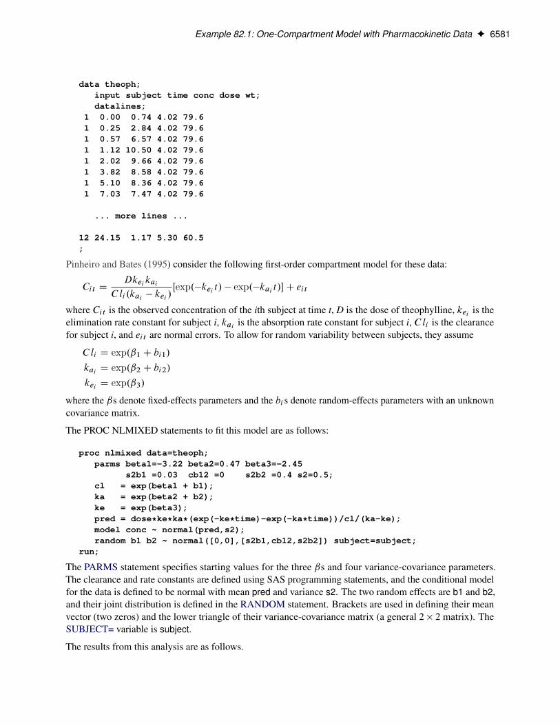
Example 82.1: One-Compartment Model with Pharmacokinetic Data F 6581
data theoph;input subject time conc dose wt;datalines;
1 0.00 0.74 4.02 79.61 0.25 2.84 4.02 79.61 0.57 6.57 4.02 79.61 1.12 10.50 4.02 79.61 2.02 9.66 4.02 79.61 3.82 8.58 4.02 79.61 5.10 8.36 4.02 79.61 7.03 7.47 4.02 79.6
... more lines ...
12 24.15 1.17 5.30 60.5;
Pinheiro and Bates (1995) consider the following first-order compartment model for these data:
Cit DDkeikai
Cli .kai � kei /Œexp.�kei t / � exp.�kai t /�C eit
where Cit is the observed concentration of the ith subject at time t, D is the dose of theophylline, kei is theelimination rate constant for subject i, kai is the absorption rate constant for subject i, Cli is the clearancefor subject i, and eit are normal errors. To allow for random variability between subjects, they assume
Cli D exp.ˇ1 C bi1/kai D exp.ˇ2 C bi2/kei D exp.ˇ3/
where the ˇs denote fixed-effects parameters and the bi s denote random-effects parameters with an unknowncovariance matrix.
The PROC NLMIXED statements to fit this model are as follows:
proc nlmixed data=theoph;parms beta1=-3.22 beta2=0.47 beta3=-2.45
s2b1 =0.03 cb12 =0 s2b2 =0.4 s2=0.5;cl = exp(beta1 + b1);ka = exp(beta2 + b2);ke = exp(beta3);pred = dose*ke*ka*(exp(-ke*time)-exp(-ka*time))/cl/(ka-ke);model conc ~ normal(pred,s2);random b1 b2 ~ normal([0,0],[s2b1,cb12,s2b2]) subject=subject;
run;
The PARMS statement specifies starting values for the three ˇs and four variance-covariance parameters.The clearance and rate constants are defined using SAS programming statements, and the conditional modelfor the data is defined to be normal with mean pred and variance s2. The two random effects are b1 and b2,and their joint distribution is defined in the RANDOM statement. Brackets are used in defining their meanvector (two zeros) and the lower triangle of their variance-covariance matrix (a general 2 � 2 matrix). TheSUBJECT= variable is subject.
The results from this analysis are as follows.
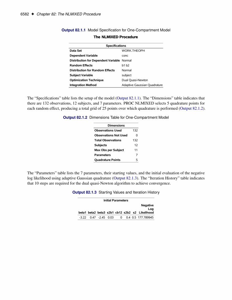
6582 F Chapter 82: The NLMIXED Procedure
Output 82.1.1 Model Specification for One-Compartment Model
The NLMIXED ProcedureThe NLMIXED Procedure
Specifications
Data Set WORK.THEOPH
Dependent Variable conc
Distribution for Dependent Variable Normal
Random Effects b1 b2
Distribution for Random Effects Normal
Subject Variable subject
Optimization Technique Dual Quasi-Newton
Integration Method Adaptive Gaussian Quadrature
The “Specifications” table lists the setup of the model (Output 82.1.1). The “Dimensions” table indicates thatthere are 132 observations, 12 subjects, and 7 parameters. PROC NLMIXED selects 5 quadrature points foreach random effect, producing a total grid of 25 points over which quadrature is performed (Output 82.1.2).
Output 82.1.2 Dimensions Table for One-Compartment Model
Dimensions
Observations Used 132
Observations Not Used 0
Total Observations 132
Subjects 12
Max Obs per Subject 11
Parameters 7
Quadrature Points 5
The “Parameters” table lists the 7 parameters, their starting values, and the initial evaluation of the negativelog likelihood using adaptive Gaussian quadrature (Output 82.1.3). The “Iteration History” table indicatesthat 10 steps are required for the dual quasi-Newton algorithm to achieve convergence.
Output 82.1.3 Starting Values and Iteration History
Initial Parameters
beta1 beta2 beta3 s2b1 cb12 s2b2 s2
NegativeLog
Likelihood
-3.22 0.47 -2.45 0.03 0 0.4 0.5 177.789945

Example 82.1: One-Compartment Model with Pharmacokinetic Data F 6583
Output 82.1.3 continued
Iteration History
Iteration Calls
NegativeLog
Likelihood DifferenceMaximumGradient Slope
1 7 177.7762 0.013697 2.87337 -63.0744
2 11 177.7643 0.011948 1.69814 -4.75239
3 14 177.7573 0.007036 1.29744 -1.97311
4 17 177.7557 0.001576 1.44141 -0.49772
5 20 177.7467 0.008988 1.13228 -0.82230
6 24 177.7464 0.000299 0.83129 -0.00244
7 27 177.7463 0.000083 0.72420 -0.00789
8 31 177.7457 0.000578 0.18002 -0.00583
9 34 177.7457 3.88E-6 0.017958 -8.25E-6
10 37 177.7457 3.222E-8 0.000143 -6.51E-8
NOTE: GCONV convergence criterion satisfied.
Output 82.1.4 Fit Statistics for One-Compartment Model
Fit Statistics
-2 Log Likelihood 355.5
AIC (smaller is better) 369.5
AICC (smaller is better) 370.4
BIC (smaller is better) 372.9
The “Fit Statistics” table lists the final optimized values of the log-likelihood function and information criteriain the “smaller is better” form (Output 82.1.4).
The “Parameter Estimates” table contains the maximum likelihood estimates of the parameters (Output 82.1.5).Both s2b1 and s2b2 are marginally significant, indicating between-subject variability in the clearances andabsorption rate constants, respectively. There does not appear to be a significant covariance between them, asseen by the estimate of cb12.
Output 82.1.5 Parameter Estimates for One-Compartment Model
Parameter Estimates
Parameter EstimateStandard
Error DF t Value Pr > |t|
95%Confidence
Limits Gradient
beta1 -3.2268 0.05950 10 -54.23 <.0001 -3.3594 -3.0942 -0.00009
beta2 0.4806 0.1989 10 2.42 0.0363 0.03745 0.9238 3.645E-7
beta3 -2.4592 0.05126 10 -47.97 <.0001 -2.5734 -2.3449 0.000039
s2b1 0.02803 0.01221 10 2.30 0.0446 0.000828 0.05524 -0.00014
cb12 -0.00127 0.03404 10 -0.04 0.9710 -0.07712 0.07458 -0.00007
s2b2 0.4331 0.2005 10 2.16 0.0561 -0.01354 0.8798 -6.98E-6
s2 0.5016 0.06837 10 7.34 <.0001 0.3493 0.6540 6.133E-6
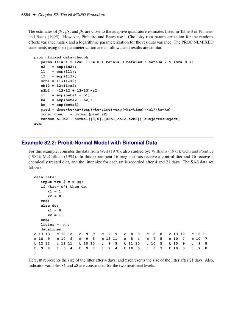
6584 F Chapter 82: The NLMIXED Procedure
The estimates of ˇ1, ˇ2, and ˇ3 are close to the adaptive quadrature estimates listed in Table 3 of Pinheiroand Bates (1995). However, Pinheiro and Bates use a Cholesky-root parameterization for the random-effects variance matrix and a logarithmic parameterization for the residual variance. The PROC NLMIXEDstatements using their parameterization are as follows, and results are similar.
proc nlmixed data=theoph;parms ll1=-1.5 l2=0 ll3=-0.1 beta1=-3 beta2=0.5 beta3=-2.5 ls2=-0.7;s2 = exp(ls2);l1 = exp(ll1);l3 = exp(ll3);s2b1 = l1*l1*s2;cb12 = l2*l1*s2;s2b2 = (l2*l2 + l3*l3)*s2;cl = exp(beta1 + b1);ka = exp(beta2 + b2);ke = exp(beta3);pred = dose*ke*ka*(exp(-ke*time)-exp(-ka*time))/cl/(ka-ke);model conc ~ normal(pred,s2);random b1 b2 ~ normal([0,0],[s2b1,cb12,s2b2]) subject=subject;
run;
Example 82.2: Probit-Normal Model with Binomial DataFor this example, consider the data from Weil (1970), also studied by: Williams (1975); Ochi and Prentice(1984); McCulloch (1994). In this experiment 16 pregnant rats receive a control diet and 16 receive achemically treated diet, and the litter size for each rat is recorded after 4 and 21 days. The SAS data setfollows:
data rats;input trt $ m x @@;if (trt='c') then do;
x1 = 1;x2 = 0;
end;else do;
x1 = 0;x2 = 1;
end;litter = _n_;datalines;
c 13 13 c 12 12 c 9 9 c 9 9 c 8 8 c 8 8 c 13 12 c 12 11c 10 9 c 10 9 c 9 8 c 13 11 c 5 4 c 7 5 c 10 7 c 10 7t 12 12 t 11 11 t 10 10 t 9 9 t 11 10 t 10 9 t 10 9 t 9 8t 9 8 t 5 4 t 9 7 t 7 4 t 10 5 t 6 3 t 10 3 t 7 0;
Here, m represents the size of the litter after 4 days, and x represents the size of the litter after 21 days. Also,indicator variables x1 and x2 are constructed for the two treatment levels.

Example 82.2: Probit-Normal Model with Binomial Data F 6585
Following McCulloch (1994), assume a latent survival model of the form
yijk D ti C ˛ij C eijk
where i indexes treatment, j indexes litter, and k indexes newborn rats within a litter. The ti representtreatment means, the ˛ij represent random litter effects assumed to be iid N.0; s2i /, and the eijk represent iidresidual errors, all on the latent scale.
Instead of observing the survival times yijk , assume that only the binary variable indicating whether yijkexceeds 0 is observed. If xij denotes the sum of these binary variables for the ith treatment and the jth litter,then the preceding assumptions lead to the following generalized linear mixed model:
xij j˛ij � Binomial.mij ; pij /
where mij is the size of each litter after 4 days and
pij D ˆ.ti C ˛ij /
The PROC NLMIXED statements to fit this model are as follows:
proc nlmixed data=rats;parms t1=1 t2=1 s1=.05 s2=1;eta = x1*t1 + x2*t2 + alpha;p = probnorm(eta);model x ~ binomial(m,p);random alpha ~ normal(0,x1*s1*s1+x2*s2*s2) subject=litter;estimate 'gamma2' t2/sqrt(1+s2*s2);predict p out=p;
run;
As in Example 82.1, the PROC NLMIXED statement invokes the procedure and the PARMS statementdefines the parameters. The parameters for this example are the two treatment means, t1 and t2, and the tworandom-effect standard deviations, s1 and s2.
The indicator variables x1 and x2 are used in the program to assign the proper mean to each observation inthe input data set as well as the proper variance to the random effects. Note that programming expressions arepermitted inside the distributional specifications, as illustrated by the random-effects variance specified here.
The ESTIMATE statement requests an estimate of 2 D t2=q1C s22 , which is a location-scale parameter
from Ochi and Prentice (1984).
The PREDICT statement constructs predictions for each observation in the input data set. For this example,predictions of p and approximate standard errors of prediction are output to a SAS data set named P. Thesepredictions are functions of the parameter estimates and the empirical Bayes estimates of the random effects˛i .
The output for this model is as follows.

6586 F Chapter 82: The NLMIXED Procedure
Output 82.2.1 Specifications, Dimensions, and Starting Values
The NLMIXED ProcedureThe NLMIXED Procedure
Specifications
Data Set WORK.RATS
Dependent Variable x
Distribution for Dependent Variable Binomial
Random Effects alpha
Distribution for Random Effects Normal
Subject Variable litter
Optimization Technique Dual Quasi-Newton
Integration Method Adaptive Gaussian Quadrature
Dimensions
Observations Used 32
Observations Not Used 0
Total Observations 32
Subjects 32
Max Obs per Subject 1
Parameters 4
Quadrature Points 7
Initial Parameters
t1 t2 s1 s2
NegativeLog
Likelihood
1 1 0.05 1 54.9362323
The “Specifications” table provides basic information about this nonlinear mixed model (Output 82.2.1). The“Dimensions” table provides counts of various variables. Note that each observation in the data comprises aseparate subject. Using the starting values in the “Parameters” table, PROC NLMIXED determines that thelog-likelihood function can be approximated with sufficient accuracy with a seven-point quadrature rule.
Output 82.2.2 Iteration History for Probit-Normal Model
Iteration History
Iteration Calls
NegativeLog
Likelihood DifferenceMaximumGradient Slope
1 4 53.9933934 0.942839 11.0326 -81.9428
2 6 52.8753530 1.11804 2.14895 -2.86277
3 9 52.6350386 0.240314 0.32996 -1.05049
4 11 52.6319939 0.003045 0.12293 -0.00672
5 14 52.6313583 0.000636 0.028246 -0.00352
6 18 52.6313174 0.000041 0.013551 -0.00023
7 21 52.6313115 5.839E-6 0.000603 -0.00001
8 24 52.6313115 9.45E-9 0.000022 -1.68E-8
NOTE: GCONV convergence criterion satisfied.

Example 82.3: Probit-Normal Model with Ordinal Data F 6587
The “Iteration History” table indicates successful convergence in 8 iterations (Output 82.2.2).
Output 82.2.3 Fit Statistics for Probit-Normal Model
Fit Statistics
-2 Log Likelihood 105.3
AIC (smaller is better) 113.3
AICC (smaller is better) 114.7
BIC (smaller is better) 119.1
The “Fit Statistics” table lists useful statistics based on the maximized value of the log likelihood (Out-put 82.2.3).
Output 82.2.4 Parameter Estimates for Probit-Normal Model
Parameter Estimates
Parameter EstimateStandard
Error DF t Value Pr > |t|
95%Confidence
Limits Gradient
t1 1.3063 0.1685 31 7.75 <.0001 0.9626 1.6499 -0.00002
t2 0.9475 0.3055 31 3.10 0.0041 0.3244 1.5705 9.283E-6
s1 0.2403 0.3015 31 0.80 0.4315 -0.3746 0.8552 0.000014
s2 1.0292 0.2988 31 3.44 0.0017 0.4198 1.6386 -3.16E-6
The “Parameter Estimates” table indicates significance of all the parameters except S1 (Output 82.2.4).
Output 82.2.5 Additional Estimates
Additional Estimates
Label EstimateStandard
Error DF t Value Pr > |t| Alpha Lower Upper
gamma2 0.6603 0.2165 31 3.05 0.0047 0.05 0.2186 1.1019
The “Additional Estimates” table displays results from the ESTIMATE statement (Output 82.2.5). Theestimate of 2 equals 0.66, agreeing with that obtained by McCulloch (1994). The standard error 0.22 iscomputed using the delta method (Billingsley 1986; Cox 1998).
Not shown is the P data set, which contains the original 32 observations and predictions of the pij .
Example 82.3: Probit-Normal Model with Ordinal DataThe data for this example are from Ezzet and Whitehead (1991), who describe a crossover experiment on twogroups of patients using two different inhaler devices (A and B). Patients from group 1 used device A for oneweek and then device B for another week. Patients from group 2 used the devices in reverse order. The dataentered as a SAS data set are as follows:

6588 F Chapter 82: The NLMIXED Procedure
data inhaler;input clarity group time freq @@;gt = group*time;sub = floor((_n_+1)/2);datalines;
1 0 0 59 1 0 1 59 1 0 0 35 2 0 1 35 1 0 0 3 3 0 1 3 1 0 0 24 0 1 2 2 0 0 11 1 0 1 11 2 0 0 27 2 0 1 27 2 0 0 2 3 0 1 22 0 0 1 4 0 1 1 4 0 0 1 1 0 1 1 4 0 0 1 2 0 1 1 1 1 0 631 1 1 63 1 1 0 13 2 1 1 13 2 1 0 40 1 1 1 40 2 1 0 15 2 1 1 153 1 0 7 1 1 1 7 3 1 0 2 2 1 1 2 3 1 0 1 3 1 1 1 4 1 0 21 1 1 2 4 1 0 1 3 1 1 1;
The response measurement, clarity, is the patients’ assessment on the clarity of the leaflet instructions for thedevices. The clarity variable is on an ordinal scale, with 1=easy, 2=only clear after rereading, 3=not veryclear, and 4=confusing. The group variable indicates the treatment group, and the time variable indicates thetime of measurement. The freq variable indicates the number of patients with exactly the same responses. Avariable gt is created to indicate a group-by-time interaction, and a variable sub is created to indicate patients.
As in the previous example and in Hedeker and Gibbons (1994), assume an underlying latent continuousvariable, here with the form
yij D ˇ0 C ˇ1gi C ˇ2tj C ˇ3gi tj C ui C eij
where i indexes patient and j indexes the time period, gi indicates groups, tj indicates time, ui is a patient-level normal random effect, and eij are iid normal errors. The ˇs are unknown coefficients to be estimated.
Instead of observing yij , however, you observe only whether it falls in one of the four intervals: (�1, 0),(0, I1), (I1, I1 + I2), or (I1 + I2,1), where I1 and I2 are both positive. The resulting category is the valueassigned to the clarity variable.
The following code sets up and fits this ordinal probit model:
proc nlmixed data=inhaler corr ecorr;parms b0=0 b1=0 b2=0 b3=0 sd=1 i1=1 i2=1;bounds i1 > 0, i2 > 0;eta = b0 + b1*group + b2*time + b3*gt + u;if (clarity=1) then p = probnorm(-eta);else if (clarity=2) then
p = probnorm(i1-eta) - probnorm(-eta);else if (clarity=3) then
p = probnorm(i1+i2-eta) - probnorm(i1-eta);else p = 1 - probnorm(i1+i2-eta);if (p > 1e-8) then ll = log(p);else ll = -1e20;model clarity ~ general(ll);random u ~ normal(0,sd*sd) subject=sub;replicate freq;estimate 'thresh2' i1;estimate 'thresh3' i1 + i2;estimate 'icc' sd*sd/(1+sd*sd);
run;

Example 82.3: Probit-Normal Model with Ordinal Data F 6589
The PROC NLMIXED statement specifies the input data set and requests correlations both for the parameterestimates (CORR option) and for the additional estimates specified with ESTIMATE statements (ECORRoption).
The parameters as defined in the PARMS statement are as follows: b0 (overall intercept), b1 (group maineffect), B2 (time main effect), b3 (group-by-time interaction), sd (standard deviation of the random effect), i1(increment between first and second thresholds), and i2 (increment between second and third thresholds).The BOUNDS statement restricts i1 and i2 to be positive.
The SAS programming statements begin by defining the linear predictor eta, which is a linear combination ofthe b parameters and a single random effect u. The next statements define the ordinal likelihood according tothe clarity variable, eta, and the increment variables. An error trap is included in case the likelihood becomestoo small.
A general log-likelihood specification is used in the MODEL statement, and the RANDOM statement definesthe random effect u to have standard deviation sd and subject variable sub. The REPLICATE statementindicates that data for each subject should be replicated according to the freq variable.
The ESTIMATE statements specify the second and third thresholds in terms of the increment variables (thefirst threshold is assumed to equal zero for model identifiability). Also computed is the intraclass correlation.
The output is as follows.
Output 82.3.1 Specifications for Ordinal Data Model
The NLMIXED ProcedureThe NLMIXED Procedure
Specifications
Data Set WORK.INHALER
Dependent Variable clarity
Distribution for Dependent Variable General
Random Effects u
Distribution for Random Effects Normal
Subject Variable sub
Replicate Variable freq
Optimization Technique Dual Quasi-Newton
Integration Method Adaptive Gaussian Quadrature
The “Specifications” table echoes some primary information specified for this nonlinear mixed model(Output 82.3.1). Because the log-likelihood function was expressed with SAS programming statements, thedistribution is displayed as General in the “Specifications” table.
The “Dimensions” table reveals a total of 286 subjects, which is the sum of the values of the FREQ variablefor the second time point. Five quadrature points are selected for log-likelihood evaluation (Output 82.3.2).
Output 82.3.2 Dimensions Table for Ordinal Data Model
Dimensions
Observations Used 38
Observations Not Used 0
Total Observations 38
Subjects 286
Max Obs per Subject 2
Parameters 7
Quadrature Points 5

6590 F Chapter 82: The NLMIXED Procedure
Output 82.3.3 Parameter Starting Values and Negative Log Likelihood
Initial Parameters
b0 b1 b2 b3 sd i1 i2
NegativeLog
Likelihood
0 0 0 0 1 1 1 538.484276
The “Parameters” table lists the simple starting values for this problem (Output 82.3.3). The “IterationHistory” table indicates successful convergence in 13 iterations (Output 82.3.4).
Output 82.3.4 Iteration History
Iteration History
Iteration Calls
NegativeLog
Likelihood DifferenceMaximumGradient Slope
1 4 476.3825 62.10176 43.7506 -1431.40
2 7 463.2282 13.15431 14.2465 -106.753
3 9 458.5281 4.70008 48.3132 -33.0389
4 11 450.9757 7.552383 22.6010 -40.9954
5 14 448.0127 2.963033 14.8688 -16.7453
6 17 447.2452 0.767549 7.77419 -2.26743
7 19 446.7277 0.517483 3.79353 -1.59278
8 22 446.5183 0.209396 0.86864 -0.37801
9 26 446.5145 0.003745 0.32857 -0.02356
10 29 446.5133 0.001187 0.056778 -0.00183
11 32 446.5133 0.000027 0.010785 -0.00004
12 35 446.5133 3.956E-6 0.004922 -5.41E-6
13 38 446.5133 1.989E-7 0.000470 -4E-7
NOTE: GCONV convergence criterion satisfied.
Output 82.3.5 Fit Statistics for Ordinal Data Model
Fit Statistics
-2 Log Likelihood 893.0
AIC (smaller is better) 907.0
AICC (smaller is better) 910.8
BIC (smaller is better) 932.6
The “Fit Statistics” table lists the log likelihood and information criteria for model comparisons (Out-put 82.3.5).
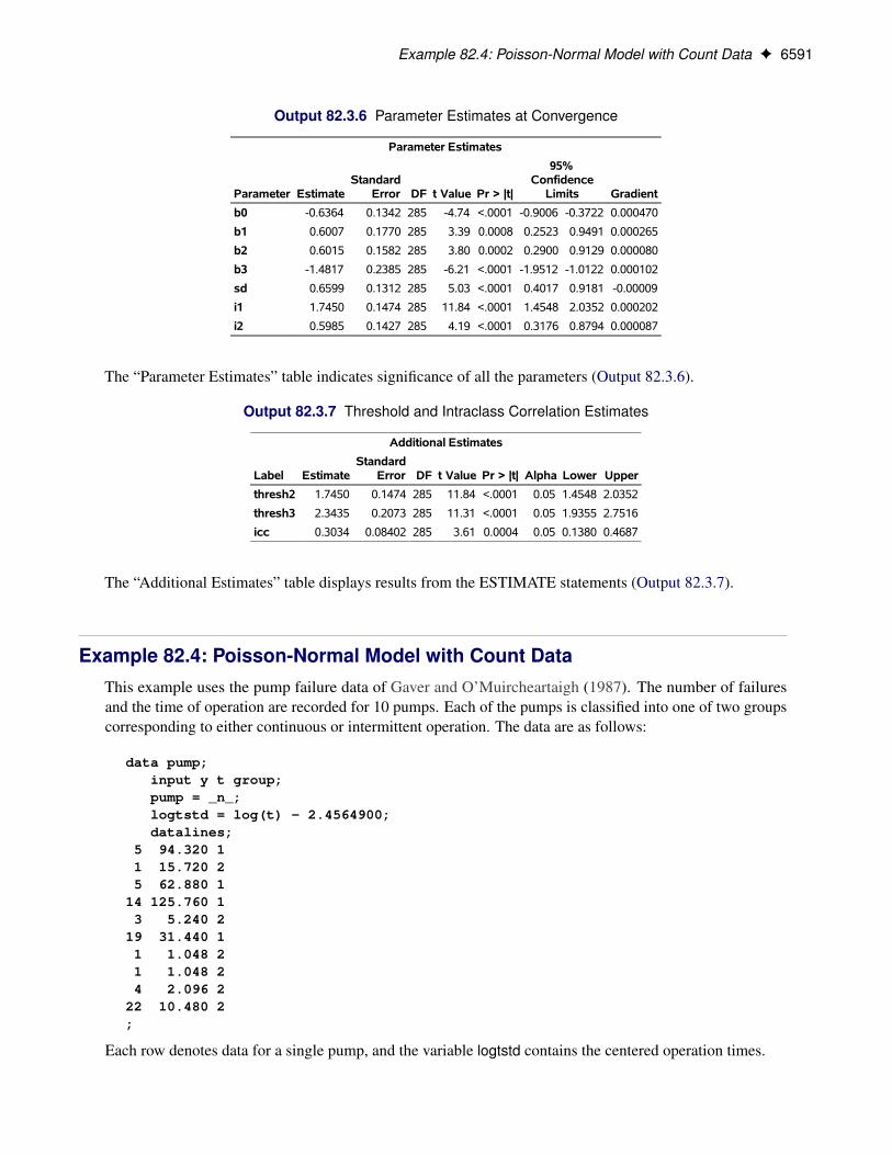
Example 82.4: Poisson-Normal Model with Count Data F 6591
Output 82.3.6 Parameter Estimates at Convergence
Parameter Estimates
Parameter EstimateStandard
Error DF t Value Pr > |t|
95%Confidence
Limits Gradient
b0 -0.6364 0.1342 285 -4.74 <.0001 -0.9006 -0.3722 0.000470
b1 0.6007 0.1770 285 3.39 0.0008 0.2523 0.9491 0.000265
b2 0.6015 0.1582 285 3.80 0.0002 0.2900 0.9129 0.000080
b3 -1.4817 0.2385 285 -6.21 <.0001 -1.9512 -1.0122 0.000102
sd 0.6599 0.1312 285 5.03 <.0001 0.4017 0.9181 -0.00009
i1 1.7450 0.1474 285 11.84 <.0001 1.4548 2.0352 0.000202
i2 0.5985 0.1427 285 4.19 <.0001 0.3176 0.8794 0.000087
The “Parameter Estimates” table indicates significance of all the parameters (Output 82.3.6).
Output 82.3.7 Threshold and Intraclass Correlation Estimates
Additional Estimates
Label EstimateStandard
Error DF t Value Pr > |t| Alpha Lower Upper
thresh2 1.7450 0.1474 285 11.84 <.0001 0.05 1.4548 2.0352
thresh3 2.3435 0.2073 285 11.31 <.0001 0.05 1.9355 2.7516
icc 0.3034 0.08402 285 3.61 0.0004 0.05 0.1380 0.4687
The “Additional Estimates” table displays results from the ESTIMATE statements (Output 82.3.7).
Example 82.4: Poisson-Normal Model with Count DataThis example uses the pump failure data of Gaver and O’Muircheartaigh (1987). The number of failuresand the time of operation are recorded for 10 pumps. Each of the pumps is classified into one of two groupscorresponding to either continuous or intermittent operation. The data are as follows:
data pump;input y t group;pump = _n_;logtstd = log(t) - 2.4564900;datalines;
5 94.320 11 15.720 25 62.880 1
14 125.760 13 5.240 2
19 31.440 11 1.048 21 1.048 24 2.096 2
22 10.480 2;
Each row denotes data for a single pump, and the variable logtstd contains the centered operation times.

6592 F Chapter 82: The NLMIXED Procedure
Letting yij denote the number of failures for the jth pump in the ith group, Draper (1996) considers thefollowing hierarchical model for these data:
yij j�ij � Poisson.�ij /
log �ij D ˛i C ˇi .log tij � log t /C eijeij j�
2� Normal.0; �2/
The model specifies different intercepts and slopes for each group, and the random effect is a mechanism foraccounting for overdispersion.
The corresponding PROC NLMIXED statements are as follows:
proc nlmixed data=pump;parms logsig 0 beta1 1 beta2 1 alpha1 1 alpha2 1;if (group = 1) then eta = alpha1 + beta1*logtstd + e;else eta = alpha2 + beta2*logtstd + e;lambda = exp(eta);model y ~ poisson(lambda);random e ~ normal(0,exp(2*logsig)) subject=pump;estimate 'alpha1-alpha2' alpha1-alpha2;estimate 'beta1-beta2' beta1-beta2;
run;
The selected output is as follows.
Output 82.4.1 Dimensions Table for Poisson-Normal Model
The NLMIXED ProcedureThe NLMIXED Procedure
Dimensions
Observations Used 10
Observations Not Used 0
Total Observations 10
Subjects 10
Max Obs per Subject 1
Parameters 5
Quadrature Points 5
The “Dimensions” table indicates that data for 10 pumps are used with one observation for each (Out-put 82.4.1).

Example 82.4: Poisson-Normal Model with Count Data F 6593
Output 82.4.2 Iteration History for Poisson-Normal Model
Iteration History
Iteration Calls
NegativeLog
Likelihood DifferenceMaximumGradient Slope
1 4 30.6986932 2.162768 5.10725 -91.6020
2 9 30.0255468 0.673146 2.76174 -11.0489
3 12 29.7263250 0.299222 2.99040 -2.36048
4 16 28.7390263 0.987299 2.07443 -3.93678
5 18 28.3161933 0.422833 0.61253 -0.63084
6 21 28.0956400 0.220553 0.46216 -0.52684
7 24 28.0438024 0.051838 0.40505 -0.10018
8 27 28.0357134 0.008089 0.13506 -0.01875
9 30 28.0339250 0.001788 0.026279 -0.00514
10 33 28.0338744 0.000051 0.004020 -0.00012
11 36 28.0338727 1.681E-6 0.002864 -5.09E-6
12 39 28.0338724 3.199E-7 0.000147 -6.87E-7
13 42 28.0338724 2.532E-9 0.000017 -5.75E-9
NOTE: GCONV convergence criterion satisfied.
The “Iteration History” table indicates successful convergence in 13 iterations (Output 82.4.2).
Output 82.4.3 Fit Statistics for Poisson-Normal Model
Fit Statistics
-2 Log Likelihood 56.1
AIC (smaller is better) 66.1
AICC (smaller is better) 81.1
BIC (smaller is better) 67.6
The “Fit Statistics” table lists the final log likelihood and associated information criteria (Output 82.4.3).
Output 82.4.4 Parameter Estimates and Additional Estimates
Parameter Estimates
Parameter EstimateStandard
Error DF t Value Pr > |t|
95%Confidence
Limits Gradient
logsig -0.3161 0.3213 9 -0.98 0.3508 -1.0429 0.4107 -0.00002
beta1 -0.4256 0.7473 9 -0.57 0.5829 -2.1162 1.2649 -0.00002
beta2 0.6097 0.3814 9 1.60 0.1443 -0.2530 1.4725 -1.61E-6
alpha1 2.9644 1.3826 9 2.14 0.0606 -0.1632 6.0921 -5.25E-6
alpha2 1.7992 0.5492 9 3.28 0.0096 0.5568 3.0415 -5.73E-6
Additional Estimates
Label EstimateStandard
Error DF t Value Pr > |t| Alpha Lower Upper
alpha1-alpha2 1.1653 1.4855 9 0.78 0.4529 0.05 -2.1952 4.5257
beta1-beta2 -1.0354 0.8389 9 -1.23 0.2484 0.05 -2.9331 0.8623

6594 F Chapter 82: The NLMIXED Procedure
The “Parameter Estimates” and “Additional Estimates” tables list the maximum likelihood estimates for eachof the parameters and two differences (Output 82.4.4). The point estimates for the mean parameters agreefairly closely with the Bayesian posterior means reported by Draper (1996); however, the likelihood-basedstandard errors are roughly half the Bayesian posterior standard deviations. This is most likely due to the factthat the Bayesian standard deviations account for the uncertainty in estimating �2, whereas the likelihoodvalues plug in its estimated value. This downward bias can be corrected somewhat by using the t9 distributionshown here.
Example 82.5: Failure Time and Frailty ModelIn this example an accelerated failure time model with proportional hazard is fitted with and without randomeffects. The data are from the “Getting Started” example of PROC LIFEREG; see Chapter 69, “The LIFEREGProcedure.” Thirty-eight patients are divided into two groups of equal size, and different pain relievers areassigned to each group. The outcome reported is the time in minutes until headache relief. The variablecensor indicates whether relief was observed during the course of the observation period (censor = 0) orwhether the observation is censored (censor = 1). The SAS DATA step for these data is as follows:
data headache;input minutes group censor @@;patient = _n_;datalines;
11 1 0 12 1 0 19 1 0 19 1 019 1 0 19 1 0 21 1 0 20 1 021 1 0 21 1 0 20 1 0 21 1 020 1 0 21 1 0 25 1 0 27 1 030 1 0 21 1 1 24 1 1 14 2 016 2 0 16 2 0 21 2 0 21 2 023 2 0 23 2 0 23 2 0 23 2 025 2 1 23 2 0 24 2 0 24 2 026 2 1 32 2 1 30 2 1 30 2 032 2 1 20 2 1;
In modeling survival data, censoring of observations must be taken into account carefully. In this example,only right censoring occurs. If g.t;ˇ/, h.t;ˇ/, and G.t;ˇ/ denote the density of failure, the hazard function,and the survival distribution function at time t, respectively, then the log likelihood can be written as
l.ˇI t/ DXi2Uu
log g.ti ;ˇ/CXi2Uc
logG.ti ;ˇ/
D
Xi2Uu
log h.ti ;ˇ/CnXiD1
logG.ti ;ˇ/
(See Cox and Oakes 1984, Ch. 3.) In these expressions Uu is the set of uncensored observations, Uc is theset of censored observations, and n denotes the total sample size.

Example 82.5: Failure Time and Frailty Model F 6595
The proportional hazards specification expresses the hazard in terms of a baseline hazard, multiplied by aconstant. In this example the hazard is that of a Weibull model and is parameterized as h.t;ˇ/ D ˛.˛t/ �1
and ˛ D expf�x0ˇg.
The linear predictor is set equal to the intercept in the reference group (group = 2); this defines thebaseline hazard. The corresponding distribution of survival past time t is G.t;ˇ/ D expf�.˛t/ g. SeeCox and Oakes (1984, Table 2.1) and the section “Supported Distributions” in Chapter 69, “The LIFEREGProcedure,” for this and other survival distribution models and various parameterizations.
The following NLMIXED statements fit this accelerated failure time model and estimate the cumulativedistribution function of time to headache relief:
proc nlmixed data=headache;bounds gamma > 0;linp = b0 - b1*(group-2);alpha = exp(-linp);G_t = exp(-(alpha*minutes)**gamma);g = gamma*alpha*((alpha*minutes)**(gamma-1))*G_t;ll = (censor=0)*log(g) + (censor=1)*log(G_t);model minutes ~ general(ll);predict 1-G_t out=cdf;
run;
Output 82.5.1 Specifications Table for Fixed-Effects Failure Time Model
The NLMIXED ProcedureThe NLMIXED Procedure
Specifications
Data Set WORK.HEADACHE
Dependent Variable minutes
Distribution for Dependent Variable General
Optimization Technique Dual Quasi-Newton
Integration Method None
The “Specifications” table shows that no integration is required, since the model does not contain randomeffects (Output 82.5.1).
Output 82.5.2 Negative Log Likelihood with Default Starting Values
Initial Parameters
gamma b0 b1
NegativeLog
Likelihood
1 1 1 263.990327
No starting values were given for the three parameters. The NLMIXED procedure assigns the default valueof 1.0 in this case. The negative log likelihood based on these starting values is shown in Output 82.5.2.

6596 F Chapter 82: The NLMIXED Procedure
Output 82.5.3 Iteration History for Fixed-Effects Failure Time Model
Iteration History
Iteration Calls
NegativeLog
Likelihood DifferenceMaximumGradient Slope
1 4 169.2443 94.74602 22.5599 -2230.83
2 8 142.8735 26.3708 14.8863 -3.64643
3 11 140.6337 2.239814 11.2523 -9.49454
4 15 122.8907 17.74304 19.4496 -2.50807
5 17 121.3970 1.493699 13.8558 -4.55427
6 20 120.6238 0.773116 13.6706 -1.38064
7 22 119.2782 1.345647 15.7801 -1.69072
8 26 116.2713 3.006871 26.9403 -3.25290
9 30 109.4274 6.843925 19.8838 -6.92890
10 35 103.2981 6.129298 12.1565 -4.96054
11 40 101.6862 1.611863 14.2487 -4.34059
12 42 100.0279 1.658364 11.6985 -13.2049
13 46 99.9189048 0.108971 3.60255 -0.55176
14 49 99.8738836 0.045021 0.17071 -0.16645
15 52 99.8736392 0.000244 0.050822 -0.00041
16 55 99.8736351 4.071E-6 0.000705 -6.9E-6
17 58 99.8736351 6.1E-10 4.768E-6 -1.23E-9
NOTE: GCONV convergence criterion satisfied.
The “Iteration History” table shows that the procedure converges after 17 iterations and 34 evaluations of theobjective function (Output 82.5.3).
Output 82.5.4 Fit Statistics and Parameter Estimates
Fit Statistics
-2 Log Likelihood 199.7
AIC (smaller is better) 205.7
AICC (smaller is better) 206.5
BIC (smaller is better) 210.7
Parameter Estimates
Parameter EstimateStandard
Error DF t Value Pr > |t|
95%Confidence
Limits Gradient
gamma 4.7128 0.6742 38 6.99 <.0001 3.3479 6.0777 5.327E-8
b0 3.3091 0.05885 38 56.23 <.0001 3.1900 3.4283 -4.77E-6
b1 -0.1933 0.07856 38 -2.46 0.0185 -0.3523 -0.03426 -1.22E-6
The parameter estimates and their standard errors shown in Output 82.5.4 are identical to those obtained withthe LIFEREG procedure and the following statements:

Example 82.5: Failure Time and Frailty Model F 6597
proc lifereg data=headache;class group;model minutes*censor(1) = group / dist=weibull;output out=new cdf=prob;
run;
The t statistic and confidence limits are based on 38 degrees of freedom. The LIFEREG procedure computesz intervals for the parameter estimates.
For the two groups you obtain
b̨.group D 1/ D expf�3:3091C 0:1933g D 0:04434b̨.group D 2/ D expf�3:3091g D 0:03655
The probabilities of headache relief by t minutes are estimated as
1 �G.t; group D 1/ D 1 � expf�.0:04434 � t /4:7128g
1 �G.t; group D 2/ D 1 � expf�.0:03655 � t /4:7128g
These probabilities, calculated at the observed times, are shown for the two groups in Output 82.5.5 andprinted with the following statements:
proc print data=cdf;var group censor patient minutes pred;
run;
Since the slope estimate is negative with p-value of 0.0185, you can infer that pain reliever 1 leads to overallsignificantly faster relief, but the estimated probabilities give no information about patient-to-patient variationwithin and between groups. For example, while pain reliever 1 provides faster relief overall, some patientsin group 2 might respond more quickly than some patients in group 1. A frailty model enables you toaccommodate and estimate patient-to-patient variation in health status by introducing random effects into asubject’s hazard function.

6598 F Chapter 82: The NLMIXED Procedure
Output 82.5.5 Estimated Cumulative Distribution Function
Obs group censor patient minutes Pred
1 1 0 1 11 0.03336
2 1 0 2 12 0.04985
3 1 0 3 19 0.35975
4 1 0 4 19 0.35975
5 1 0 5 19 0.35975
6 1 0 6 19 0.35975
7 1 0 7 21 0.51063
8 1 0 8 20 0.43325
9 1 0 9 21 0.51063
10 1 0 10 21 0.51063
11 1 0 11 20 0.43325
12 1 0 12 21 0.51063
13 1 0 13 20 0.43325
14 1 0 14 21 0.51063
15 1 0 15 25 0.80315
16 1 0 16 27 0.90328
17 1 0 17 30 0.97846
18 1 1 18 21 0.51063
19 1 1 19 24 0.73838
20 2 0 20 14 0.04163
21 2 0 21 16 0.07667
22 2 0 22 16 0.07667
23 2 0 23 21 0.24976
24 2 0 24 21 0.24976
25 2 0 25 23 0.35674
26 2 0 26 23 0.35674
27 2 0 27 23 0.35674
28 2 0 28 23 0.35674
29 2 1 29 25 0.47982
30 2 0 30 23 0.35674
31 2 0 31 24 0.41678
32 2 0 32 24 0.41678
33 2 1 33 26 0.54446
34 2 1 34 32 0.87656
35 2 1 35 30 0.78633
36 2 0 36 30 0.78633
37 2 1 37 32 0.87656
38 2 1 38 20 0.20414
The following statements model the hazard for patient i in terms of ˛i D expf�x0iˇ � zig, where zi is a(normal) random patient effect. Notice that the only difference from the previous NLMIXED statements arethe RANDOM statement and the addition of z in the linear predictor. The empirical Bayes estimates of therandom effect (RANDOM statement), the parameter estimates (ODS OUTPUT statement), and the estimatedcumulative distribution function (PREDICT statement) are saved to subsequently graph the patient-specificdistribution functions.

Example 82.5: Failure Time and Frailty Model F 6599
ods output ParameterEstimates=est;proc nlmixed data=headache;
bounds gamma > 0;linp = b0 - b1*(group-2) + z;alpha = exp(-linp);G_t = exp(-(alpha*minutes)**gamma);g = gamma*alpha*((alpha*minutes)**(gamma-1))*G_t;ll = (censor=0)*log(g) + (censor=1)*log(G_t);model minutes ~ general(ll);random z ~ normal(0,exp(2*logsig)) subject=patient out=EB;predict 1-G_t out=cdf;
run;
Output 82.5.6 Specifications for Random Frailty Model
The NLMIXED ProcedureThe NLMIXED Procedure
Specifications
Data Set WORK.HEADACHE
Dependent Variable minutes
Distribution for Dependent Variable General
Random Effects z
Distribution for Random Effects Normal
Subject Variable patient
Optimization Technique Dual Quasi-Newton
Integration Method Adaptive Gaussian Quadrature
The “Specifications” table shows that the objective function is computed by adaptive Gaussian quadraturebecause of the presence of random effects (compare Output 82.5.6 and Output 82.5.1). The “Dimensions”table reports that nine quadrature points are being used to integrate over the random effects (Output 82.5.7).
Output 82.5.7 Dimensions Table for Random Frailty Model
Dimensions
Observations Used 38
Observations Not Used 0
Total Observations 38
Subjects 38
Max Obs per Subject 1
Parameters 4
Quadrature Points 9
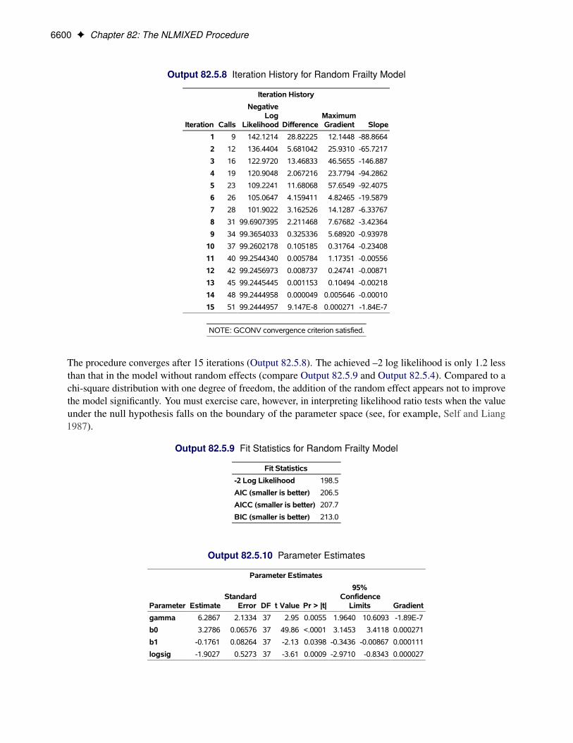
6600 F Chapter 82: The NLMIXED Procedure
Output 82.5.8 Iteration History for Random Frailty Model
Iteration History
Iteration Calls
NegativeLog
Likelihood DifferenceMaximumGradient Slope
1 9 142.1214 28.82225 12.1448 -88.8664
2 12 136.4404 5.681042 25.9310 -65.7217
3 16 122.9720 13.46833 46.5655 -146.887
4 19 120.9048 2.067216 23.7794 -94.2862
5 23 109.2241 11.68068 57.6549 -92.4075
6 26 105.0647 4.159411 4.82465 -19.5879
7 28 101.9022 3.162526 14.1287 -6.33767
8 31 99.6907395 2.211468 7.67682 -3.42364
9 34 99.3654033 0.325336 5.68920 -0.93978
10 37 99.2602178 0.105185 0.31764 -0.23408
11 40 99.2544340 0.005784 1.17351 -0.00556
12 42 99.2456973 0.008737 0.24741 -0.00871
13 45 99.2445445 0.001153 0.10494 -0.00218
14 48 99.2444958 0.000049 0.005646 -0.00010
15 51 99.2444957 9.147E-8 0.000271 -1.84E-7
NOTE: GCONV convergence criterion satisfied.
The procedure converges after 15 iterations (Output 82.5.8). The achieved –2 log likelihood is only 1.2 lessthan that in the model without random effects (compare Output 82.5.9 and Output 82.5.4). Compared to achi-square distribution with one degree of freedom, the addition of the random effect appears not to improvethe model significantly. You must exercise care, however, in interpreting likelihood ratio tests when the valueunder the null hypothesis falls on the boundary of the parameter space (see, for example, Self and Liang1987).
Output 82.5.9 Fit Statistics for Random Frailty Model
Fit Statistics
-2 Log Likelihood 198.5
AIC (smaller is better) 206.5
AICC (smaller is better) 207.7
BIC (smaller is better) 213.0
Output 82.5.10 Parameter Estimates
Parameter Estimates
Parameter EstimateStandard
Error DF t Value Pr > |t|
95%Confidence
Limits Gradient
gamma 6.2867 2.1334 37 2.95 0.0055 1.9640 10.6093 -1.89E-7
b0 3.2786 0.06576 37 49.86 <.0001 3.1453 3.4118 0.000271
b1 -0.1761 0.08264 37 -2.13 0.0398 -0.3436 -0.00867 0.000111
logsig -1.9027 0.5273 37 -3.61 0.0009 -2.9710 -0.8343 0.000027
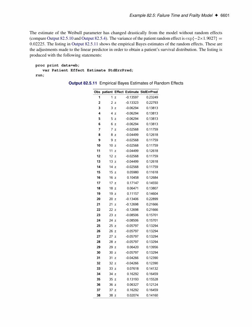
Example 82.5: Failure Time and Frailty Model F 6601
The estimate of the Weibull parameter has changed drastically from the model without random effects(compare Output 82.5.10 and Output 82.5.4). The variance of the patient random effect is expf�2�1:9027g D0:02225. The listing in Output 82.5.11 shows the empirical Bayes estimates of the random effects. These arethe adjustments made to the linear predictor in order to obtain a patient’s survival distribution. The listing isproduced with the following statements:
proc print data=eb;var Patient Effect Estimate StdErrPred;
run;
Output 82.5.11 Empirical Bayes Estimates of Random Effects
Obs patient Effect Estimate StdErrPred
1 1 z -0.13597 0.23249
2 2 z -0.13323 0.22793
3 3 z -0.06294 0.13813
4 4 z -0.06294 0.13813
5 5 z -0.06294 0.13813
6 6 z -0.06294 0.13813
7 7 z -0.02568 0.11759
8 8 z -0.04499 0.12618
9 9 z -0.02568 0.11759
10 10 z -0.02568 0.11759
11 11 z -0.04499 0.12618
12 12 z -0.02568 0.11759
13 13 z -0.04499 0.12618
14 14 z -0.02568 0.11759
15 15 z 0.05980 0.11618
16 16 z 0.10458 0.12684
17 17 z 0.17147 0.14550
18 18 z 0.06471 0.13807
19 19 z 0.11157 0.14604
20 20 z -0.13406 0.22899
21 21 z -0.12698 0.21666
22 22 z -0.12698 0.21666
23 23 z -0.08506 0.15701
24 24 z -0.08506 0.15701
25 25 z -0.05797 0.13294
26 26 z -0.05797 0.13294
27 27 z -0.05797 0.13294
28 28 z -0.05797 0.13294
29 29 z 0.06420 0.13956
30 30 z -0.05797 0.13294
31 31 z -0.04266 0.12390
32 32 z -0.04266 0.12390
33 33 z 0.07618 0.14132
34 34 z 0.16292 0.16459
35 35 z 0.13193 0.15528
36 36 z 0.06327 0.12124
37 37 z 0.16292 0.16459
38 38 z 0.02074 0.14160

6602 F Chapter 82: The NLMIXED Procedure
The predicted values and patient-specific survival distributions can be plotted with the SAS code that follows:
proc transpose data=est(keep=estimate)out=trest(rename=(col1=gamma col2=b0 col3=b1));
run;
data pred;merge eb(keep=estimate) headache(keep=patient group);array pp{2} pred1-pred2;if _n_ = 1 then set trest(keep=gamma b0 b1);do time=11 to 32;
linp = b0 - b1*(group-2) + estimate;pp{group} = 1-exp(- (exp(-linp)*time)**gamma);symbolid = patient+1;output;
end;keep pred1 pred2 time patient;
run;
data pred;merge pred
cdf(where = (group=1)rename = (pred=pcdf1 minutes=minutes1)keep = pred minutes group)
cdf(where = (group=2)rename = (pred=pcdf2 minutes=minutes2)keep = pred minutes group);
drop group;run;
proc sgplot data=pred noautolegend;label minutes1='Minutes to Headache Relief'
pcdf1 ='Estimated Patient-specific CDF';series x=time y=pred1 /
group=patientlineattrs=(pattern=solid color=black);
series x=time y=pred2 /group=patientlineattrs=(pattern=dash color=black);
scatter x=minutes1 y=pcdf1 /markerattrs=(symbol=CircleFilled size=9);
scatter x=minutes2 y=pcdf2 /markerattrs=(symbol=Circle size=9);
run;
The separation of the distribution functions by groups is evident in Output 82.5.12. Most of the distributionsof patients in the first group are to the left of the distributions in the second group. The separation is notcomplete, however. Several patients who are assigned the second pain reliever experience headache reliefmore quickly than patients assigned to the first group.

Example 82.5: Failure Time and Frailty Model F 6603
Output 82.5.12 Patient-Specific CDFs and Predicted Values. Pain Reliever 1: Solid Lines, Closed Circles;Pain Reliever 2: Dashed Lines, Open Circles.

6604 F Chapter 82: The NLMIXED Procedure
Example 82.6: Simulated Nested Linear Random-Effects ModelThis simulation study example demonstrates how to fit a hierarchical model with PROC NLMIXED by usinga simple two-level nested linear model. In this example, the data are generated from a simple two-levelnested hierarchical normal model (Littell et al. 2006). Here the conditional distribution of the responsevariable, given the random effects, is normal. The mean of this conditional normal distribution is a linearfunction of a fixed parameter and the random effects. In this simulation, only the intercept is used as a fixedparameter. Also, the first-level random effects are assumed to follow a normal distribution. Similarly, thesecond-level random effects that are nested within the first level follow a normal distribution. The model canbe represented as follows:
yij jˇ0; vi ; vj.i/ � N.�ij ; �2/
�ij D ˇ0 C vi C vj.i/
vi � N.0; �2a /
vj.i/ � N.0; �2b /
The simulation code is as follows:
%let na = 100;%let nb = 5;%let nr = 2;data nested;
do A = 1 to &na;err1 = 3*rannor(339205);do B = 1 to &nb;
err2 = 2*rannor(0);do rep = 1 to &nr;
err3 = 1*rannor(0);resp = 10 + err1 + err2 + err3;output;
end;end;
end;run;
You can use PROC NLMIXED to fit the preceding nested model as follows by using two RANDOMstatements:
proc nlmixed data = nested;bounds vara >=0, varb_a >=0;mean = intercept + aeffect + beffect;model resp ~ normal (mean, s2);random aeffect ~ normal(0,vara) subject = A;random beffect ~ normal(0,varb_a) subject = B(A);
run;
The MODEL statement specifies the response variable distribution as normal. The linear relationship betweenthe mean of this normal distribution and the fixed and random effects is specified by using a SAS programmingstatement. The BOUNDS statement specifies the nonnegative constraints on the variance parameters.
PROC NLMIXED with multiple RANDOM statements is used to fit hierarchical (nested) models. In thisexample, two RANDOM statements are used to fit a two-level nested model. The first RANDOM statement

Example 82.6: Simulated Nested Linear Random-Effects Model F 6605
identifies aeffect as the first-level random effect, vi , and it is followed by the subject variable A. The subjectvariable A indexes the number of distinct and independent subjects at the first level. Then the secondRANDOM statement identifies the beffect, vj.i/, as the second-level random effect, which is nested withinthe first level. The subject variable specification in the second RANDOM statement defines the nestedstructure. In this example, the subject variable B is nested within A.
The results from the analysis follow.
Output 82.6.1 Model Specifications for a Two-Level Nested Model
The NLMIXED ProcedureThe NLMIXED Procedure
Specifications
Data Set WORK.NESTED
Dependent Variable resp
Distribution for Dependent Variable Normal
Random Effects aeffect, beffect
Distribution for Random Effects Normal, Normal
Subject Variables A, B
Optimization Technique Dual Quasi-Newton
Integration Method Adaptive Gaussian Quadrature
The “Specifications” table (Output 82.6.1) lists the setup of the nested model. It lists all the random effectsand their distribution along with the SUBJECT= variable in the nested sequence. Random effects that arelisted in the specifications table are separated by a comma, indicating that aeffect is the first-level randomeffect, followed by the second-level random effect, beffect, which is nested within the first level. The samescheme applies to the distribution and subject items in the table. In this example, aeffect is the random effectfor the first level and is specified using the subject variable A, which follows a normal distribution. Thenbeffect is the random effect for the second level, which is nested within the first level; it is specified using thesubject variable B, which also follows a normal distribution.
The “Dimensions” table (Output 82.6.2) follows the same nested flow to exhibit the model dimensions. Itindicates that 1,000 observations are used. There are 100 first-level subjects and 500 second-level subjects,because each first-level subject is contained by five nested second-level subjects. For this model, PROCNLMIXED selects one quadrature point to fit the model.
Output 82.6.2 Dimensions Table for a Two-Level Nested Model
Dimensions
Observations Used 1000
Observations Not Used 0
Total Observations 1000
Subjects [A] 100
Max Obs per Subject 10
Subjects [B] 500
Max Obs per Subject 2
Parameters 4
Quadrature Points 1

6606 F Chapter 82: The NLMIXED Procedure
A total of 15 steps are required to achieve convergence. They are shown in the “Iteration History” table(Output 82.6.3).
Output 82.6.3 Iteration History
Iteration History
Iteration Calls
NegativeLog
Likelihood DifferenceMaximumGradient Slope
1 12 2982.0141 2695.598 215.363 -87641.4
2 37 2462.0898 519.9243 518.335 -346.648
3 43 2144.0047 318.0852 60.9954 -2483.38
4 49 2108.7720 35.23267 56.3198 -64.4603
5 61 2098.5627 10.20936 43.0728 -7.79282
6 67 2094.2091 4.353502 34.1536 -20.0831
7 73 2090.2802 3.928941 26.4378 -5.86557
8 80 2089.3443 0.935937 15.0337 -2.41721
9 86 2088.1107 1.233618 20.3762 -0.59126
10 98 2072.7699 15.3408 5.02630 -1.53248
11 105 2068.5424 4.227408 28.6084 -2.25950
12 112 2066.4439 2.09858 9.01353 -2.53321
13 119 2065.8127 0.63118 3.73621 -0.50717
14 126 2065.7590 0.053646 1.02924 -0.07232
15 133 2065.7550 0.00406 0.36114 -0.00578
16 139 2065.7502 0.004798 0.27897 -0.00171
NOTE: GCONV convergence criterion satisfied.
The “Parameter Estimates” table (Output 82.6.4) contains the maximum likelihood estimates of the parameters.You can see from this table that the intercept and the s2 variables are very close to the simulation parameters.Also, both variances are very close to the simulation parameters.
Output 82.6.4 Parameter Estimates for a Two-Level Nested Model
Parameter Estimates
Parameter EstimateStandard
Error DF t Value Pr > |t|
95%Confidence
Limits Gradient
vara 9.2198 1.4299 498 6.45 <.0001 6.4104 12.0292 0.022612
varb_a 3.6997 0.2973 498 12.44 <.0001 3.1156 4.2839 0.008443
intercept 10.1546 0.3171 498 32.02 <.0001 9.5315 10.7776 -0.04079
s2 0.9661 0.06102 498 15.83 <.0001 0.8462 1.0860 -0.31590

Example 82.7: Overdispersion Hierarchical Nonlinear Mixed Model F 6607
Example 82.7: Overdispersion Hierarchical Nonlinear Mixed ModelThis example describes the overdispersion hierarchical nonlinear mixed model that is given in Ghebretinsaeet al. (2013). In this experiment, 24 rats are divided into four groups and receive a daily oral dose of1,2-dimethylhydrazine dihydrochloride in three dose levels (low, medium, and high) and a vehicle control.In addition, an extra group of three animals receive a positive control. All 27 animals are euthanized 3hours after the last dose is administered. For each animal, a cell suspension is prepared, and from eachcell suspension, three replicate samples are prepared for scoring. Using a semi-automated scoring system,50 randomly selected cells from each sample are scored per animal for DNA damage. The comet assaymethodology is used to detect this DNA damage. In this methodology, the DNA damage is measured by thedistance of DNA migration from the perimeter of the comet head to the last visible point in the tail. Thisdistance is defined as the tail length and is observed for the 150 cells from each animal. The data are availablein the Sashelp library. In order to use the dose levels as regressors in PROC NLMIXED, you need to createindicator variables for each dose level. The following DATA step creates indicator variables for the doselevels:
data comet;set sashelp.comet;L = 0; M = 0; H = 0; PC = 0;if (dose = 1.25) then L = 1;if (dose = 2.50) then M = 1;if (dose = 5.00) then H = 1;if (dose = 200) then PC = 1;
run;
Ghebretinsae et al. (2013) suggest a Weibull distribution to model the outcomes (tail lengths). Note that thedata exhibit the nested nature because of the three replicate samples from each cell. Also, the 50 cells fromeach rat are correlated. To account for the dependency of these 150 correlated cells from each rat, two levelsof normally distributed nested random effects are used. Let yijk be the tail length that is observed in the kthcell from the jth sample of the ith rat. Then the suggested two-level nested model can be described as follows:
yijkjri ; sj.i/ �Weibull.�; �ijk/
�ijk D exp.ˇ0 C ˇ1Lijk C ˇ2Mijk C ˇ3Hijk C ˇ4PCi C ri C sj.i//ri � N.0; d1/
sj.i/ � N.0; d2/
This model is referred to as the nested Weibull model in the rest of the example. The parameters of theWeibull distribution, � and �ijk , are known as the shape and scale parameters, respectively. Based on thismodel specification, the conditional expectation of the response variable, given the random effects, is anonlinear function of fixed and random effects. The nonlinear relationship can be written as
E.yijkjri ; sj.i// D��1�C 1
��1=�
ijk
D
��1�C 1
��e.ˇ0Cˇ1LijkCˇ2MijkCˇ3HijkCˇ4PCiCriCsj.i//
�1=�These expected values can be obtained using the PREDICT statement in PROC NLMIXED, and they areuseful for validating the model fitting. The specified nested Weibull model can be fitted using the followingPROC NLMIXED statements:

6608 F Chapter 82: The NLMIXED Procedure
proc nlmixed data = comet;parms b0 = -25 b1 = -10 b2 = -10 b3 = -10 b4 = -10 rho = 10;bounds sd1 >=0, sd2 >=0;mu = b0+ b1*L+ b2*M+ b3*H+ b4*PC + rateff + sampeff;term = (length**rho)*exp(mu);llike = log(rho) + (rho-1)*log(length) + mu - term;model length ~ general(llike);random ratEff ~ normal(0,sd1) subject = rat;random sampEff ~ normal(0,sd2) subject = sample(rat);predict gamma(1+(1/rho))/(exp(mu)**(1/rho)) out = p1;
run;
Note that the two-parameter Weibull density function is given by
f .yI �; �/ D ��y��1e��y�
This implies that the log likelihood is
l.�; �Iy/ D log.�/C log.�/C .� � 1/ log.y/ � �y�
A general log-likelihood specification is used in the MODEL statement to specify the preceding log of theWeibull density. The linear combination of the parameters, b0 to b4, and the two random effects, RatEffand SampEff, is defined using the linear predictor MU in the first SAS programming statement. Then, thenext two SAS programming statements together define the log of the Weibull density function. The firstRANDOM statement defines the first level of the random effect, ri , by using RatEff. Then, the secondRANDOM statement defines the second level of the random effect, sj.i/, nested within the first level by usingSampEff. Both random-effects distributions are specified as normal with mean 0 and variance sd1 and sd2for the first and second levels, respectively. The selected output from this model is shown in Output 82.7.1,Output 82.7.2, and Output 82.7.3.
Output 82.7.1 Model Specification for Nested Weibull Model
The NLMIXED ProcedureThe NLMIXED Procedure
Specifications
Data Set WORK.COMET
Dependent Variable Length
Distribution for Dependent Variable General
Random Effects rateff, sampeff
Distribution for Random Effects Normal, Normal
Subject Variables Rat, Sample
Optimization Technique Dual Quasi-Newton
Integration Method Adaptive Gaussian Quadrature
The “Specifications” table shows that RatEff is the first-level random effect, specified by the subject variableRat, and it follows a normal distribution (Output 82.7.1). Similarly, SampEff is the second-level randomeffect, nested in RatEff and specified by the subject variable Sample, and it follows a normal distribution.

Example 82.7: Overdispersion Hierarchical Nonlinear Mixed Model F 6609
Output 82.7.2 Dimensions Table for Nested Weibull Model
Dimensions
Observations Used 4050
Observations Not Used 0
Total Observations 4050
Subjects [Rat] 27
Max Obs per Subject 150
Subjects [Sample] 81
Max Obs per Subject 50
Parameters 8
Quadrature Points 1
The “Dimensions” table indicates that 4,050 observations are used in the analysis (Output 82.7.2). It alsoindicates that there are 27 rats and that 81 samples are nested within the rats. As explained earlier, threesamples are selected randomly from each rat, so a total of 81 (27 times 3) samples are used in the analysis.
Output 82.7.3 Parameter Estimates for Nested Weibull Model
Parameter Estimates
Parameter EstimateStandard
Error DF t Value Pr > |t|
95%Confidence
Limits Gradient
b0 -15.6346 0.2627 79 -59.52 <.0001 -16.1575 -15.1117 -0.21455
b1 -4.4912 0.2345 79 -19.15 <.0001 -4.9581 -4.0244 -0.12563
b2 -4.5865 0.2186 79 -20.98 <.0001 -5.0216 -4.1514 0.20926
b3 -4.8188 0.2188 79 -22.02 <.0001 -5.2543 -4.3833 0.088666
b4 -3.4834 0.2664 79 -13.08 <.0001 -4.0136 -2.9532 -0.18096
rho 4.9558 0.05881 79 84.27 <.0001 4.8388 5.0729 -1.18121
sd1 0.02454 0.04601 79 0.53 0.5953 -0.06704 0.1161 -0.75888
sd2 0.3888 0.07106 79 5.47 <.0001 0.2473 0.5302 -0.79003
The “Parameter Estimates” table list the maximum likelihood estimates of the parameters along with theirstandard errors (Output 82.7.3). The estimates are fairly close to the estimates that are given in Ghebretinsaeet al. (2013), who use a gamma distribution for the Sample random effects instead of the normal distributionas in the preceding model. Note that the parameters ˇ1, ˇ2, and ˇ3 represent the effects of low, medium,and high doses, respectively, when compared to the vehicle control. Similarly, ˇ4 is the parameter thatcorresponds to the effect of positive control when compared to vehicle control. The p-value indicatesthat the point estimates of all these parameters, ˇ1 to ˇ4, are significant; this implies that the toxicity of1,2-dimethylhydrazine dihydrochloride is significant at different dose levels.
In the nested Weibull model, the scale parameter, �ijk , is random because it is a function of random effects.This implies that the model assumes that each observation is drawn from a different Weibull distribution.Molenberghs et al. (2010) indicate that this way of modeling leads to an overdispersed Weibull model.Ghebretinsae et al. (2013) use the random-effects mechanism to account for this overdispersion. The

6610 F Chapter 82: The NLMIXED Procedure
overdispersed Weibull model can be written as follows:
yijkjri ; sj.i/; �ijk �Weibull.�; �ijk/
�ijk D �ijk exp.ˇ0 C ˇ1Lijk C ˇ2Mijk C ˇ3Hijk C ˇ4PCi C ri C sj.i//�ijk � gamma.˛; 1=˛/
ri � N.0; d1/
sj.i/ � N.0; d2/
This model is referred to as the nested Weibull overdispersion model in the rest of this example. Again,in this model, the shape parameter, �ijk , is the function of the normally distributed random effects, riand sj.i/, along with other random effects, �ijk . Further, the model assumes that �ijk follow a gammadistribution. Note that the random effects, ri and sj.i/, account for the cluster effect of the observationsfrom the same sample that is nested within a rat, whereas �ijk account for the overdispersion in the data.Molenberghs et al. (2010) integrate out the overdispersion random effects, �ijk , from the joint distributionf .yijkj�ijk; ri ; sj.i//g.�ijkj˛/ and provide the conditional density of yijkjri ; sj.i/. The conditional densityfollows:
f .yijkjri ; sj.i// D�y��1ij e.ˇ0Cˇ1LijkCˇ2MijkCˇ3HijkCˇ4PCiCriCsj.i//�
1C 1˛y�ij e
.ˇ0Cˇ1LijkCˇ2MijkCˇ3HijkCˇ4PCiCriCsj.i//�˛C1
Again, in this case, the conditional expectation of the response variable, given the random effects, is anonlinear function of the fixed and random effects. Molenberghs et al. (2010) provide this nonlinearrelationship as follows:
E.yijkjri ; sj.i// D��˛ � 1
�
���1�C 1
��1˛e.ˇ0Cˇ1LijkCˇ2MijkCˇ3HijkCˇ4PCiCriCsj.i//
�1=��.˛/
As indicated previously, these values are useful for validating the fit of the model, and they can be obtainedusing a PREDICT statement in PROC NLMIXED. Using the preceding conditional distribution of response,given the random effects and the random-effects distribution, PROC NLMIXED fits the two-level nestedWeibull overdispersion model by using the following statements:
ods select ParameterEstimates;proc nlmixed data = comet;
parms b0 = -25 b1 = -10 b2 = -10 b3 = -10 b4 = -10 alpha = 1 rho = 10;bounds sd1 >=0, sd2 >=0;mu = b0+ b1*L+ b2*M+ b3*H+ b4*PC + rateff + sampeff;num = rho*((length)**(rho-1))*exp(mu);den = (1+(((length)**rho)*exp(mu))/alpha)**(alpha+1);llike = log(num/den);model length ~ general(llike);random rateff ~ normal(0,sd1) subject = rat;random sampeff ~ normal(0,sd2) subject = sample(rat);predict (gamma(alpha-(1/rho))*gamma(1+(1/rho)))
/(gamma(alpha)*((exp(mu)/alpha)**(1/rho))) out = p2;run;
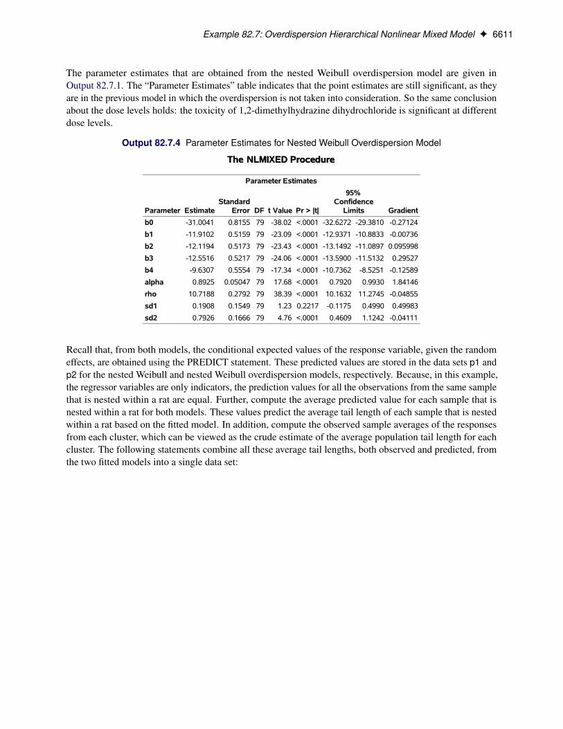
Example 82.7: Overdispersion Hierarchical Nonlinear Mixed Model F 6611
The parameter estimates that are obtained from the nested Weibull overdispersion model are given inOutput 82.7.1. The “Parameter Estimates” table indicates that the point estimates are still significant, as theyare in the previous model in which the overdispersion is not taken into consideration. So the same conclusionabout the dose levels holds: the toxicity of 1,2-dimethylhydrazine dihydrochloride is significant at differentdose levels.
Output 82.7.4 Parameter Estimates for Nested Weibull Overdispersion Model
The NLMIXED ProcedureThe NLMIXED Procedure
Parameter Estimates
Parameter EstimateStandard
Error DF t Value Pr > |t|
95%Confidence
Limits Gradient
b0 -31.0041 0.8155 79 -38.02 <.0001 -32.6272 -29.3810 -0.27124
b1 -11.9102 0.5159 79 -23.09 <.0001 -12.9371 -10.8833 -0.00736
b2 -12.1194 0.5173 79 -23.43 <.0001 -13.1492 -11.0897 0.095998
b3 -12.5516 0.5217 79 -24.06 <.0001 -13.5900 -11.5132 0.29527
b4 -9.6307 0.5554 79 -17.34 <.0001 -10.7362 -8.5251 -0.12589
alpha 0.8925 0.05047 79 17.68 <.0001 0.7920 0.9930 1.84146
rho 10.7188 0.2792 79 38.39 <.0001 10.1632 11.2745 -0.04855
sd1 0.1908 0.1549 79 1.23 0.2217 -0.1175 0.4990 0.49983
sd2 0.7926 0.1666 79 4.76 <.0001 0.4609 1.1242 -0.04111
Recall that, from both models, the conditional expected values of the response variable, given the randomeffects, are obtained using the PREDICT statement. These predicted values are stored in the data sets p1 andp2 for the nested Weibull and nested Weibull overdispersion models, respectively. Because, in this example,the regressor variables are only indicators, the prediction values for all the observations from the same samplethat is nested within a rat are equal. Further, compute the average predicted value for each sample that isnested within a rat for both models. These values predict the average tail length of each sample that is nestedwithin a rat based on the fitted model. In addition, compute the observed sample averages of the responsesfrom each cluster, which can be viewed as the crude estimate of the average population tail length for eachcluster. The following statements combine all these average tail lengths, both observed and predicted, fromthe two fitted models into a single data set:
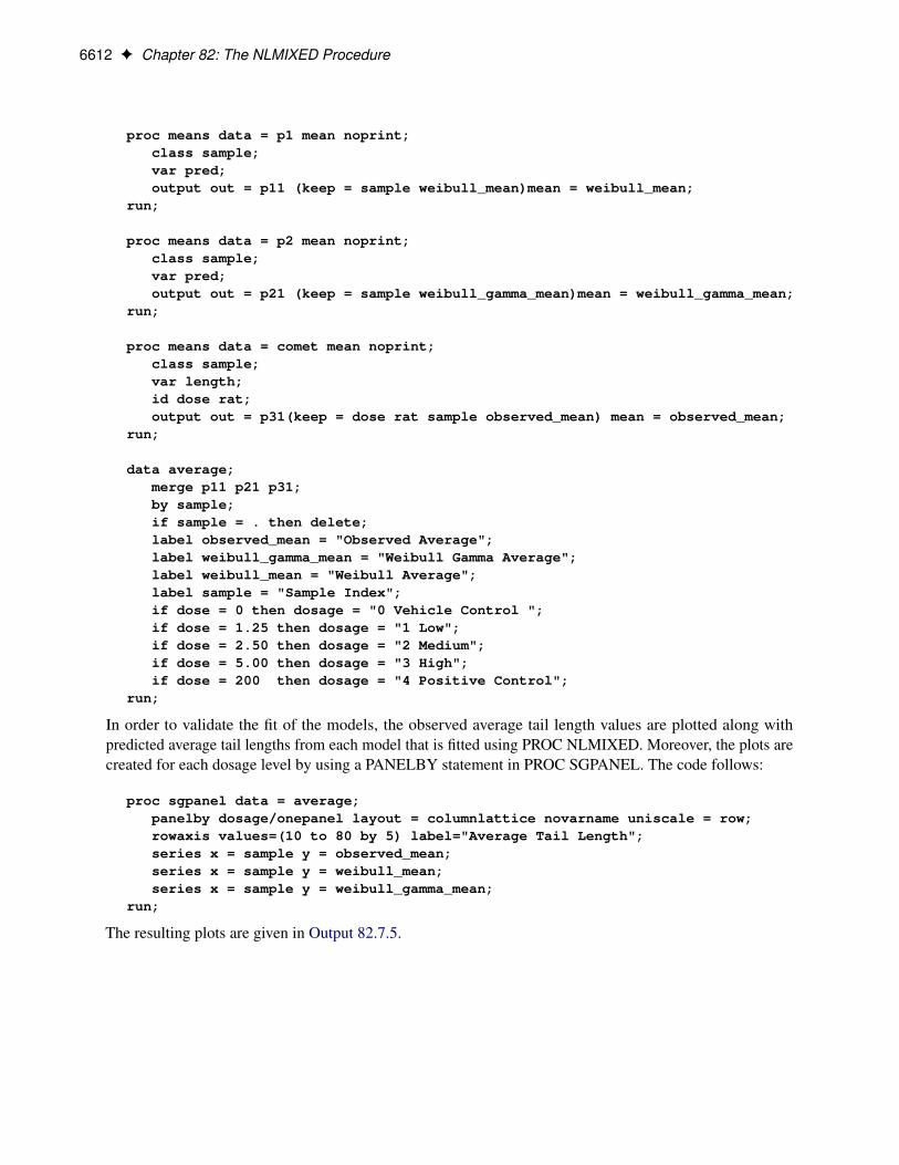
6612 F Chapter 82: The NLMIXED Procedure
proc means data = p1 mean noprint;class sample;var pred;output out = p11 (keep = sample weibull_mean)mean = weibull_mean;
run;
proc means data = p2 mean noprint;class sample;var pred;output out = p21 (keep = sample weibull_gamma_mean)mean = weibull_gamma_mean;
run;
proc means data = comet mean noprint;class sample;var length;id dose rat;output out = p31(keep = dose rat sample observed_mean) mean = observed_mean;
run;
data average;merge p11 p21 p31;by sample;if sample = . then delete;label observed_mean = "Observed Average";label weibull_gamma_mean = "Weibull Gamma Average";label weibull_mean = "Weibull Average";label sample = "Sample Index";if dose = 0 then dosage = "0 Vehicle Control ";if dose = 1.25 then dosage = "1 Low";if dose = 2.50 then dosage = "2 Medium";if dose = 5.00 then dosage = "3 High";if dose = 200 then dosage = "4 Positive Control";
run;
In order to validate the fit of the models, the observed average tail length values are plotted along withpredicted average tail lengths from each model that is fitted using PROC NLMIXED. Moreover, the plots arecreated for each dosage level by using a PANELBY statement in PROC SGPANEL. The code follows:
proc sgpanel data = average;panelby dosage/onepanel layout = columnlattice novarname uniscale = row;rowaxis values=(10 to 80 by 5) label="Average Tail Length";series x = sample y = observed_mean;series x = sample y = weibull_mean;series x = sample y = weibull_gamma_mean;
run;
The resulting plots are given in Output 82.7.5.

References F 6613
Output 82.7.5 Comparison of Nested Weibull Model and Nested Weibull Overdispersion Model
You can see from the plots that the observed averages of the tail lengths from each sample that is nestedwithin a rat are closer to the predicted averages of the nested Weibull overdispersion model than to thepredicted averages of the nested Weibull model.
References
Abramowitz, M., and Stegun, I. A., eds. (1972). Handbook of Mathematical Functions with Formulas,Graphs, and Mathematical Tables. 10th printing. New York: Dover.
Anderson, D. A., and Aitkin, M. (1985). “Variance Component Models with Binary Response: InterviewerVariability.” Journal of the Royal Statistical Society, Series B 47:203–210.
Beal, S. L., and Sheiner, L. B. (1982). “Estimating Population Kinetics.” CRC Critical Reviews in BiomedicalEngineering 8:195–222.
Beal, S. L., and Sheiner, L. B. (1988). “Heteroscedastic Nonlinear Regression.” Technometrics 30:327–338.

6614 F Chapter 82: The NLMIXED Procedure
Beal, S. L., and Sheiner, L. B. (1992). NONMEM User’s Guide. San Francisco: NONMEM Project Group,University of California, San Francisco.
Beale, E. M. L. (1972). “A Derivation of Conjugate Gradients.” In Numerical Methods for NonlinearOptimization, edited by F. A. Lootsma, 39–43. London: Academic Press.
Beitler, P. J., and Landis, J. R. (1985). “A Mixed-Effects Model for Categorical Data.” Biometrics 41:991–1000.
Billingsley, P. (1986). Probability and Measure. 2nd ed. New York: John Wiley & Sons.
Booth, J. G., and Hobert, J. P. (1998). “Standard Errors of Prediction in Generalized Linear Mixed Models.”Journal of the American Statistical Association 93:262–272.
Breslow, N. E., and Clayton, D. G. (1993). “Approximate Inference in Generalized Linear Mixed Models.”Journal of the American Statistical Association 88:9–25.
Burnham, K. P., and Anderson, D. R. (1998). Model Selection and Inference: A Practical Information-Theoretic Approach. New York: Springer-Verlag.
Cox, C. (1998). “Delta Method.” In Encyclopedia of Biostatistics, edited by P. Armitage, and T. Colton. NewYork: John Wiley & Sons.
Cox, D. R., and Oakes, D. (1984). Analysis of Survival Data. London: Chapman & Hall.
Cramer, J. S. (1986). Econometric Applications of Maximum Likelihood Methods. Cambridge: CambridgeUniversity Press.
Crouch, E. A. C., and Spiegelman, D. (1990). “The Evaluation of Integrals of the FormR1�1
f .t/ exp.�t2/dt :Application to Logistic-Normal Models.” Journal of the American Statistical Association 85:464–469.
Davidian, M., and Gallant, A. R. (1993). “The Nonlinear Mixed Effects Model with a Smooth RandomEffects Density.” Biometrika 80:475–488.
Davidian, M., and Giltinan, D. M. (1995). Nonlinear Models for Repeated Measurement Data. New York:Chapman & Hall.
Dennis, J. E., Gay, D. M., and Welsch, R. E. (1981). “An Adaptive Nonlinear Least-Squares Algorithm.”ACM Transactions on Mathematical Software 7:348–368.
Dennis, J. E., and Mei, H. H. W. (1979). “Two New Unconstrained Optimization Algorithms Which UseFunction and Gradient Values.” Journal of Optimization Theory and Applications 28:453–482.
Dennis, J. E., and Schnabel, R. B. (1983). Numerical Methods for Unconstrained Optimization and NonlinearEquations. Englewood Cliffs, NJ: Prentice-Hall.
Diggle, P. J., Liang, K.-Y., and Zeger, S. L. (1994). Analysis of Longitudinal Data. Oxford: Clarendon Press.
Draper, D. (1996). “Discussion of the Paper by Lee and Nelder.” Journal of the Royal Statistical Society,Series B 58:662–663.
Draper, N. R., and Smith, H. (1981). Applied Regression Analysis. 2nd ed. New York: John Wiley & Sons.
Engel, B., and Keen, A. (1992). A Simple Approach for the Analysis of Generalized Linear Mixed Models,vol. LWA-92-6. Wageningen, Netherlands: Agricultural Mathematics Group (GLW-DLO).

References F 6615
Eskow, E., and Schnabel, R. B. (1991). “Algorithm 695: Software for a New Modified Cholesky Factorization.”ACM Transactions on Mathematical Software 17:306–312.
Ezzet, F., and Whitehead, J. (1991). “A Random Effects Model for Ordinal Responses from a CrossoverTrial.” Statistics in Medicine 10:901–907.
Fletcher, R. (1987). Practical Methods of Optimization. 2nd ed. Chichester, UK: John Wiley & Sons.
Galecki, A. T. (1998). “NLMEM: New SAS/IML Macro for Hierarchical Nonlinear Models.” ComputerMethods and Programs in Biomedicine 55:207–216.
Gallant, A. R. (1987). Nonlinear Statistical Models. New York: John Wiley & Sons.
Gaver, D. P., and O’Muircheartaigh, I. G. (1987). “Robust Empirical Bayes Analysis of Event Rates.”Technometrics 29:1–15.
Gay, D. M. (1983). “Subroutines for Unconstrained Minimization.” ACM Transactions on MathematicalSoftware 9:503–524.
Ghebretinsae, A. H., Faes, C., Molenberghs, G., De Boeck, M., and Geys, H. (2013). “A Bayesian,Generalized Frailty Model for Comet Assays.” Journal of Biopharmaceutical Statistics 23:618–636.
Gilmour, A. R., Anderson, R. D., and Rae, A. L. (1985). “The Analysis of Binomial Data by GeneralizedLinear Mixed Model.” Biometrika 72:593–599.
Goldstein, H. (1991). “Nonlinear Multilevel Models, with an Application to Discrete Response Data.”Biometrika 78:45–51.
Golub, G. H., and Welsch, J. H. (1969). “Calculation of Gaussian Quadrature Rules.” MathematicalComputing 23:221–230.
Harville, D. A., and Mee, R. W. (1984). “A Mixed-Model Procedure for Analyzing Ordered CategoricalData.” Biometrics 40:393–408.
Hedeker, D., and Gibbons, R. D. (1994). “A Random Effects Ordinal Regression Model for MultilevelAnalysis.” Biometrics 50:933–944.
Hurvich, C. M., and Tsai, C.-L. (1989). “Regression and Time Series Model Selection in Small Samples.”Biometrika 76:297–307.
Lin, X., and Breslow, N. E. (1996). “Bias Correction in Generalized Linear Mixed Models with MultipleComponents of Dispersion.” Journal of the American Statistical Association 91:1007–1016.
Lindstrom, M. J., and Bates, D. M. (1990). “Nonlinear Mixed Effects Models for Repeated Measures Data.”Biometrics 46:673–687.
Littell, R. C., Milliken, G. A., Stroup, W. W., Wolfinger, R. D., and Schabenberger, O. (2006). SAS for MixedModels. 2nd ed. Cary, NC: SAS Institute Inc.
Liu, Q., and Pierce, D. A. (1994). “A Note on Gauss-Hermite Quadrature.” Biometrika 81:624–629.
Longford, N. T. (1994). “Logistic Regression with Random Coefficients.” Computational Statistics and DataAnalysis 17:1–15.

6616 F Chapter 82: The NLMIXED Procedure
McCulloch, C. E. (1994). “Maximum Likelihood Variance Components Estimation for Binary Data.” Journalof the American Statistical Association 89:330–335.
McGilchrist, C. A. (1994). “Estimation in Generalized Mixed Models.” Journal of the Royal StatisticalSociety, Series B 56:61–69.
Molenberghs, G., Verbeke, G., Demetrio, C. G. B., and Vieira, A. M. C. (2010). “A Family of GeneralizedLinear Models for Repeated Measures with Normal and Conjugate Random Effects.” Statistical Science25:325–347.
Moré, J. J. (1978). “The Levenberg-Marquardt Algorithm: Implementation and Theory.” In Lecture Notes inMathematics, vol. 30, edited by G. A. Watson, 105–116. Berlin: Springer-Verlag.
Moré, J. J., and Sorensen, D. C. (1983). “Computing a Trust-Region Step.” SIAM Journal on Scientific andStatistical Computing 4:553–572.
Ochi, Y., and Prentice, R. L. (1984). “Likelihood Inference in a Correlated Probit Regression Model.”Biometrika 71:531–543.
Pierce, D. A., and Sands, B. R. (1975). Extra-Bernoulli Variation in Binary Data. Technical Report 46,Department of Statistics, Oregon State University.
Pinheiro, J. C., and Bates, D. M. (1995). “Approximations to the Log-Likelihood Function in the NonlinearMixed-Effects Model.” Journal of Computational and Graphical Statistics 4:12–35.
Polak, E. (1971). Computational Methods in Optimization. New York: Academic Press.
Powell, M. J. D. (1977). “Restart Procedures for the Conjugate Gradient Method.” Mathematical Program-ming 12:241–254.
Pringle, R. M., and Rayner, A. A. (1971). Generalized Inverse Matrices with Applications to Statistics. NewYork: Hafner Publishing.
Rodriguez, G., and Goldman, N. (1995). “An Assessment of Estimation Procedures for Multilevel Modelswith Binary Response.” Journal of the Royal Statistical Society, Series A 158:73–89.
Roe, D. J. (1997). “Comparison of Population Pharmacokinetic Modeling Methods Using Simulated Data:Results from the Population Modeling Workgroup.” Statistics in Medicine 16:1241–1262.
Schall, R. (1991). “Estimation in Generalized Linear Models with Random Effects.” Biometrika 78:719–727.
Schittkowski, K., and Stoer, J. (1979). “A Factorization Method for the Solution of Constrained Linear LeastSquares Problems Allowing Subsequent Data Changes.” Numerische Mathematik 31:431–463.
Self, S. G., and Liang, K.-Y. (1987). “Asymptotic Properties of Maximum Likelihood Estimators andLikelihood Ratio Tests under Nonstandard Conditions.” Journal of the American Statistical Association82:605–610.
Serfling, R. J. (1980). Approximation Theorems of Mathematical Statistics. New York: John Wiley & Sons.
Sheiner, L. B., and Beal, S. L. (1980). “Evaluation of Methods for Estimating Population PharmacokineticParameters, Part I: Michaelis-Menten Model—Routine Clinical Pharmacokinetic Data.” Journal ofPharmacokinetics and Biopharmaceutics 8:553–571.
References F 6617
Sheiner, L. B., and Beal, S. L. (1985). “Pharmacokinetic Parameter Estimates from Several Least SquaresProcedures: Superiority of Extended Least Squares.” Journal of Pharmacokinetics and Biopharmaceutics13:185–201.
Smith, S. P. (1995). “Differentiation of the Cholesky Algorithm.” Journal of Computational and GraphicalStatistics 4:134–147.
Stiratelli, R., Laird, N. M., and Ware, J. H. (1984). “Random Effects Models for Serial Observations withBinary Response.” Biometrics 40:961–971.
Vonesh, E. F. (1992). “Nonlinear Models for the Analysis of Longitudinal Data.” Statistics in Medicine11:1929–1954.
Vonesh, E. F. (1996). “A Note on Laplace’s Approximation for Nonlinear Mixed-Effects Models.” Biometrika83:447–452.
Vonesh, E. F., and Chinchilli, V. M. (1997). Linear and Nonlinear Models for the Analysis of RepeatedMeasurements. New York: Marcel Dekker.
Weil, C. S. (1970). “Selection of the Valid Number of Sampling Units and Consideration of Their Combinationin Toxicological Studies Involving Reproduction, Teratogenesis, or Carcinogenesis.” Food and CosmeticToxicology 8:177–182.
White, H. (1982). “Maximum Likelihood Estimation of Misspecified Models.” Econometrica 50:1–25.
Williams, D. A. (1975). “The Analysis of Binary Responses from Toxicological Experiments InvolvingReproduction and Teratogenicity.” Biometrics 31:949–952.
Wolfinger, R. D. (1993). “Laplace’s Approximation for Nonlinear Mixed Models.” Biometrika 80:791–795.
Wolfinger, R. D. (1997). “Comment: Experiences with the SAS Macro NLINMIX.” Statistics in Medicine16:1258–1259.
Wolfinger, R. D., and Lin, X. (1997). “Two Taylor-Series Approximation Methods for Nonlinear MixedModels.” Computational Statistics and Data Analysis 25:465–490.
Wolfinger, R. D., and O’Connell, M. A. (1993). “Generalized Linear Mixed Models: A Pseudo-likelihoodApproach.” Journal of Statistical Computation and Simulation 48:233–243.
Yuh, L., Beal, S. L., Davidian, M., Harrison, F., Hester, A., Kowalski, K., Vonesh, E., and Wolfinger, R. D.(1994). “Population Pharmacokinetic/Pharmacodynamic Methodology and Applications: A Bibliography.”Biometrics 50:566–575.
Subject Index
accelerated failure time modelNLMIXED procedure, 6594
active set methodsNLMIXED procedure, 6568
adaptive Gaussian quadratureNLMIXED procedure, 6555
arraysNLMIXED procedure, 6545
Bayes estimationNLMIXED procedure, 6555
Bernoulli distributionNLMIXED procedure, 6548
binary distributionNLMIXED procedure, 6548
binomial distributionNLMIXED procedure, 6548
boundary constraints, 6546bounds
NLMIXED procedure, 6546Broyden-Fletcher-Goldfarb-Shanno update, 6544
censoreddata, example (NLMIXED), 6595
Choleskyparameterization (NLMIXED), 6584
computational problemsNLMIXED procedure, 6572
computational resourcesNLMIXED procedure, 6576
conjugatedescent (NLMIXED), 6544gradient (NLMIXED), 6543
contrasts, 6547convergence problems
NLMIXED procedure, 6573convergence status
NLMIXED procedure, 6579covariance matrix
NLMIXED procedure, 6575, 6579
Davidon-Fletcher-Powell update, 6544degrees of freedom
NLMIXED procedure, 6531double dogleg
method (NLMIXED), 6543
empirical Bayes estimate
NLMIXED procedure, 6518, 6525, 6532, 6549,6551
empirical Bayes estimationNLMIXED procedure, 6555
empirical bayes optionsNLMIXED procedure, 6541
examples, NLMIXEDbinomial data, 6585binomial-normal model, 6524boundary specification, 6546censored data, 6595Cholesky parameterization, 6584ESTIMATE statement, 6585failure time model, 6594frailty, 6594gamma distribution, 6558general distribution, 6588, 6595, 6599getting started, 6520GLIMMIX procedure, 6558graphics, predicted profiles, 6602group-specific random effects, 6585growth curve, 6520intraclass correlation coefficient, 6588logistic-normal model, 6524multicenter clinical trial, 6524negative binomial distribution, 6559one-compartment model, 6581orange tree data, 6520Overdispersion-nested example, 6607pharmacokinetic model, 6581Poisson-normal example, 6591PREDICT statement, 6585predicted profiles, graphics, 6602probit-normal model, binomial, 6584probit-normal model, ordinal, 6587random frailty, 6599SGPLOT procedure, 6602sigma reparameterization, 6592Simulate-nested example, 6604single random effect, 6520, 6524, 6550starting values from data set, 6573theophylline data, 6580three random effects, 6550two random effects, 6550, 6581user-specified log likelihood, 6588, 6595, 6599
finite differencingNLMIXED procedure, 6534, 6566

first-order methodNLMIXED procedure, 6556
floating point errorsNLMIXED procedure, 6572
frailtyNLMIXED procedure, 6594random, example (NLMIXED), 6594
gamma distributionNLMIXED procedure, 6548
Gaussian distributionNLMIXED procedure, 6548
general distributionNLMIXED procedure, 6548
generalized inverseNLMIXED procedure, 6535
Hessian matrixNLMIXED procedure, 6536
Hessian scalingNLMIXED procedure, 6568
hierarchical model specificationNLMIXED procedure, 6559
identification variables, 6547integral approximations
NLMIXED procedure, 6539, 6555intraclass correlation coefficient
NLMIXED procedure, 6588iteration details
NLMIXED procedure, 6537iteration history
NLMIXED procedure, 6536, 6578
lag functionalityNLMIXED procedure, 6552
Lagrange multiplierNLMIXED procedure, 6568
line-search methodsNLMIXED procedure, 6536, 6537, 6570
long run timesNLMIXED procedure, 6572
maximum likelihoodNLMIXED procedure, 6519
modelspecification (NLMIXED, 6548
negative binomial distributionNLMIXED procedure, 6548
Nelder-Mead simplexmethod (NLMIXED), 6543
nested multilevel nonlinear mixed modelsNLMIXED procedure, 6554
Newton-Raphson algorithm
NLMIXED procedure, 6543Newton-Raphson algorithm with ridging
NLMIXED procedure, 6543NLMIXED procedure
accelerated failure time model, 6594active set methods, 6568adaptive Gaussian quadrature, 6555additional estimates, 6547, 6580alpha level, 6530arrays, 6545assumptions, 6553Bernoulli distribution, 6548binary distribution, 6548binomial distribution, 6548bounds, 6546Cholesky parameterization, 6584compared with other SAS procedures and macros,
6519computational problems, 6572computational resources, 6576contrasts, 6546convergence criteria, 6529, 6535, 6562convergence problems, 6573convergence status, 6579covariance matrix, 6531, 6575, 6579cross-referencing variables, 6545degrees of freedom, 6531empirical Bayes estimate, 6518, 6525, 6532,
6549, 6551empirical Bayes estimation, 6555empirical Bayes options, 6532empirical bayes options, 6541examples, see also examples, NLMIXED, 6580finite differencing, 6534, 6566first-order method, 6556fit statistics, 6579floating point errors, 6572frailty, 6594frailty model example, 6594functional convergence criteria, 6533gamma distribution, 6548Gaussian distribution, 6548general distribution, 6548generalized inverse, 6535growth curve example, 6520Hessian matrix, 6536Hessian scaling, 6535, 6568hierarchical model specification, 6559integral approximations, 6539, 6555intraclass correlation coefficient, 6588iteration details, 6537iteration history, 6536, 6578lag functionality, 6552Lagrange multiplier, 6568

line-search methods, 6536, 6537, 6570log-likelihood function, 6557logistic-normal example, 6523long run times, 6572maximum likelihood, 6519negative binomial distribution, 6548nested multilevel nonlinear mixed models, 6554Newton-Raphson algorithm with ridging, 6543normal distribution, 6548, 6550notation, 6553ODS table names, 6580optimization techniques, 6543, 6561options summary, 6527Overdispersion-nested example, 6607overflows, 6572parameter estimates, 6579parameter rescaling, 6572parameter specification, 6548pharmacokinetics example, 6580Poisson distribution, 6548Poisson-normal example, 6591precision, 6574prediction, 6549, 6576probit-normal-binomial example, 6584probit-normal-ordinal example, 6587programming statements, 6551projected gradient, 6568projected Hessian, 6568quadrature options, 6541random effects, 6550replicate subjects, 6551sandwich estimator, 6533Simulate-nested example, 6604singularity tolerances, 6542sorting of input data set, 6531, 6550stationary point, 6574step length options, 6571syntax summary, 6527termination criteria, 6529, 6562update methods, 6544
nonlinearmixed models (NLMIXED), 6518
normal distributionNLMIXED procedure, 6548, 6550
optimizationtechniques (NLMIXED), 6543, 6561
OUTQ= data set, 6541OUTR= data set, 6541Overdispersion-nested example
NLMIXED procedure, 6607overflows
NLMIXED procedure, 6572
parameter estimates
NLMIXED procedure, 6579parameter rescaling
NLMIXED procedure, 6572parameter specification
NLMIXED procedure, 6548pharmacokinetics example
NLMIXED procedure, 6580Poisson distribution
NLMIXED procedure, 6548Poisson-normal example
NLMIXED procedure, 6591precision
NLMIXED procedure, 6574prediction
NLMIXED procedure, 6549, 6576probit-normal-binomial example
NLMIXED procedure, 6584probit-normal-ordinal example
NLMIXED procedure, 6587programming statements
NLMIXED procedure, 6551projected gradient
NLMIXED procedure, 6568projected Hessian
NLMIXED procedure, 6568
quadrature optionsNLMIXED procedure, 6541
quasi-Newton, 6543
random effectsNLMIXED procedure, 6550
replicate subjectsNLMIXED procedure, 6551
sandwich estimatorNLMIXED procedure, 6533
Simulate-nested exampleNLMIXED procedure, 6604
singularity tolerancesNLMIXED procedure, 6542
stationary pointNLMIXED procedure, 6574
step length optionsNLMIXED procedure, 6571
theophylline dataexamples, NLMIXED, 6580
trust region (TR), 6543
update methodsNLMIXED procedure, 6544

Syntax Index
ABSCONV= optionPROC NLMIXED statement, 6530
ABSFCONV= optionPROC NLMIXED statement, 6530
ABSGCONV= optionPROC NLMIXED statement, 6530
ABSXCONV= optionPROC NLMIXED statement, 6530
ALPHA= optionESTIMATE statement (NLMIXED), 6547PREDICT statement (NLMIXED), 6549PROC NLMIXED statement, 6531RANDOM statement (NLMIXED), 6551
ARRAY statementNLMIXED procedure, 6545
ASINGULAR= optionPROC NLMIXED statement, 6531
BEST= optionPARMS statement (NLMIXED), 6549
BOUNDS statementNLMIXED procedure, 6546
BY statementNLMIXED procedure, 6546
BYDATA optionPARMS statement (NLMIXED), 6549
CFACTOR= optionPROC NLMIXED statement, 6531
CONTRAST statementNLMIXED procedure, 6547
CORR optionPROC NLMIXED statement, 6531
COV optionPROC NLMIXED statement, 6531
COVSING= optionPROC NLMIXED statement, 6531
DAMPSTEP option, 6571PROC NLMIXED statement, 6531
DATA= optionPARMS statement (NLMIXED), 6549PROC NLMIXED statement, 6531
DER optionPREDICT statement (NLMIXED), 6549
DF= optionCONTRAST statement (NLMIXED), 6547ESTIMATE statement (NLMIXED), 6547PREDICT statement (NLMIXED), 6549
PROC NLMIXED statement, 6531RANDOM statement (NLMIXED), 6551
DIAHES optionPROC NLMIXED statement, 6532
EBOPT optionPROC NLMIXED statement, 6532
EBSSFRAC optionPROC NLMIXED statement, 6532
EBSSTOL optionPROC NLMIXED statement, 6532
EBSTEPS optionPROC NLMIXED statement, 6532
EBSUBSTEPS optionPROC NLMIXED statement, 6532
EBTOL optionPROC NLMIXED statement, 6532
EBZSTART optionPROC NLMIXED statement, 6532
ECORR optionPROC NLMIXED statement, 6532
ECOV optionPROC NLMIXED statement, 6532
EDER optionPROC NLMIXED statement, 6533
EMPIRICAL optionPROC NLMIXED statement, 6533
ESTIMATE statementNLMIXED procedure, 6547
FCONV2= optionPROC NLMIXED statement, 6533
FCONV= optionPROC NLMIXED statement, 6533
FD= optionPROC NLMIXED statement, 6534
FDHESSIAN= optionPROC NLMIXED statement, 6534
FDIGITS= option, 6567PROC NLMIXED statement, 6535
FLOW optionPROC NLMIXED statement, 6535
FSIZE= optionPROC NLMIXED statement, 6535
G4= optionPROC NLMIXED statement, 6535
GCONV= optionPROC NLMIXED statement, 6535

HESCAL= optionPROC NLMIXED statement, 6535
HESS optionPROC NLMIXED statement, 6536
ID statementNLMIXED procedure, 6547
INHESSIAN optionPROC NLMIXED statement, 6536
INSTEP= option, 6571, 6572PROC NLMIXED statement, 6536
ITDETAILS optionPROC NLMIXED statement, 6537
LCDEACT= optionPROC NLMIXED statement, 6537
LCEPSILON= optionPROC NLMIXED statement, 6537
LCSINGULAR= optionPROC NLMIXED statement, 6537
LINESEARCH= option, 6570PROC NLMIXED statement, 6537
LIST optionPROC NLMIXED statement, 6538
LISTCODE optionPROC NLMIXED statement, 6538
LISTDEP optionPROC NLMIXED statement, 6538
LISTDER optionPROC NLMIXED statement, 6538
LOGNOTE optionPROC NLMIXED statement, 6538
LSPRECISION= optionPROC NLMIXED statement, 6538
MAXFUNC= optionPROC NLMIXED statement, 6539
MAXITER= optionPROC NLMIXED statement, 6539
MAXSTEP= optionPROC NLMIXED statement, 6539
MAXTIME= optionPROC NLMIXED statement, 6539
METHOD= optionPROC NLMIXED statement, 6540
MINITER= optionPROC NLMIXED statement, 6540
MODEL statementNLMIXED procedure, 6548
MSINGULAR= optionPROC NLMIXED statement, 6540
NLMIXED procedure, 6527syntax, 6527
NLMIXED procedure, ARRAY statement, 6545
NLMIXED procedure, BOUNDS statement, 6546NLMIXED procedure, BY statement, 6546NLMIXED procedure, CONTRAST statement, 6547
DF= option, 6547NLMIXED procedure, ESTIMATE statement, 6547
ALPHA= option, 6547DF= option, 6547
NLMIXED procedure, ID statement, 6547NLMIXED procedure, MODEL statement, 6548NLMIXED procedure, PARMS statement, 6548
BEST= option, 6549BYDATA option, 6549DATA= option, 6549
NLMIXED procedure, PREDICT statement, 6549ALPHA= option, 6549DER option, 6549DF= option, 6549
NLMIXED procedure, PROC NLMIXED statementABSCONV= option, 6530ABSFCONV= option, 6530ABSGCONV= option, 6530ABSXCONV= option, 6530ALPHA= option, 6531ASINGULAR= option, 6531CFACTOR= option, 6531CORR option, 6531COV option, 6531COVSING= option, 6531DAMPSTEP option, 6531DATA= option, 6531DF= option, 6531DIAHES option, 6532EBOPT option, 6532EBSSFRAC option, 6532EBSSTOL option, 6532EBSTEPS option, 6532EBSUBSTEPS option, 6532EBTOL option, 6532EBZSTART option, 6532ECORR option, 6532ECOV option, 6532EDER option, 6533EMPIRICAL option, 6533FCONV2= option, 6533FCONV= option, 6533FD= option, 6534FDHESSIAN= option, 6534FDIGITS= option, 6535FLOW option, 6535FSIZE= option, 6535G4= option, 6535GCONV= option, 6535HESCAL= option, 6535HESS option, 6536

INHESSIAN option, 6536INSTEP= option, 6536ITDETAILS option, 6537LCDEACT= option, 6537LCEPSILON= option, 6537LCSINGULAR= option, 6537LINESEARCH= option, 6537LIST option, 6538LISTCODE option, 6538LISTDEP option, 6538LISTDER option, 6538LOGNOTE option, 6538LSPRECISION= option, 6538MAXFUNC= option, 6539MAXITER= option, 6539MAXSTEP= option, 6539MAXTIME= option, 6539METHOD= option, 6540MINITER= option, 6540MSINGULAR= option, 6540NOAD option, 6540NOADSCALE option, 6540NOSORTSUB option, 6541NTHREADS option, 6541OPTCHECK option, 6541OUTQ= option, 6541OUTR= option, 6541QFAC option, 6541QMAX option, 6541QPOINTS option, 6541QSCALEFAC option, 6542QTOL option, 6542RESTART option, 6542SEED option, 6542SINGCHOL= option, 6542SINGHESS= option, 6542SINGSWEEP= option, 6542SINGVAR option, 6542START option, 6542SUBGRADIENT option, 6543TECHNIQUE= option, 6543TRACE option, 6544UPDATE= option, 6544VSINGULAR= option, 6544XCONV= option, 6544XREF option, 6545XSIZE= option, 6545
NLMIXED procedure, RANDOM statement, 6550ALPHA= option, 6551DF= option, 6551OUT= option, 6551
NLMIXED procedure, REPLICATE statement, 6551NOAD option
PROC NLMIXED statement, 6540
NOADSCALE optionPROC NLMIXED statement, 6540
NOSORTSUB optionPROC NLMIXED statement, 6541
NTHREADS optionPROC NLMIXED statement, 6541
OPTCHECK optionPROC NLMIXED statement, 6541
OUT= optionRANDOM statement (NLMIXED), 6551
OUTQ= optionPROC NLMIXED statement, 6541
OUTR= optionPROC NLMIXED statement, 6541
PARMS statementNLMIXED procedure, 6548
PREDICT statementNLMIXED procedure, 6549
QFAC optionPROC NLMIXED statement, 6541
QMAX optionPROC NLMIXED statement, 6541
QPOINTS optionPROC NLMIXED statement, 6541
QSCALEFAC optionPROC NLMIXED statement, 6542
QTOL optionPROC NLMIXED statement, 6542
RANDOM statementNLMIXED procedure, 6550
REPLICATE statementNLMIXED procedure, 6551
RESTART optionPROC NLMIXED statement, 6542
SEED optionPROC NLMIXED statement, 6542
SINGCHOL= optionPROC NLMIXED statement, 6542
SINGHESS= optionPROC NLMIXED statement, 6542
SINGSWEEP= optionPROC NLMIXED statement, 6542
SINGVAR optionPROC NLMIXED statement, 6542
START optionPROC NLMIXED statement, 6542
SUBGRADIENT optionPROC NLMIXED statement, 6543
TECHNIQUE= option

PROC NLMIXED statement, 6543TRACE option
PROC NLMIXED statement, 6544
UPDATE= optionPROC NLMIXED statement, 6544
VSINGULAR= optionPROC NLMIXED statement, 6544
XCONV= optionPROC NLMIXED statement, 6544
XREF optionPROC NLMIXED statement, 6545
XSIZE= optionPROC NLMIXED statement, 6545


![[Concord] [Warrior Series 6519] Battle in the East. the German Army in Russia (2008)](https://static.fdocuments.in/doc/165x107/577cd63e1a28ab9e789bea0c/concord-warrior-series-6519-battle-in-the-east-the-german-army-in-russia.jpg)

![CMA BDHH 6519 E0-8 PA1 [Kompatibilitetsläge] · CMA-BDHH/6519/E0-8 Electrical specification: Frequency range 1800: 1710-1880 MHz 1900: 1850-1990 MHz 2100: 1920-2170 MHz Polarization](https://static.fdocuments.in/doc/165x107/5f350f6e3fc2f219b25d8c9f/cma-bdhh-6519-e0-8-pa1-kompatibilitetslge-cma-bdhh6519e0-8-electrical-specification.jpg)