The NLMIXED Procedure - Worcester Polytechnic … Chapter 46. The NLMIXED Procedure 5 1004 125 5...
87
Chapter 46 The NLMIXED Procedure Chapter Table of Contents OVERVIEW ................................... 2421 Introduction ................................... 2421 Literature on Nonlinear Mixed Models ..................... 2421 PROC NLMIXED Compared with Other SAS Procedures and Macros .... 2422 GETTING STARTED .............................. 2423 Nonlinear Growth Curves with Gaussian Data ................. 2423 Logistic-Normal Model with Binomial Data .................. 2427 SYNTAX ..................................... 2431 PROC NLMIXED Statement .......................... 2432 ARRAY Statement ............................... 2448 BOUNDS Statement .............................. 2449 BY Statement .................................. 2450 CONTRAST Statement ............................. 2450 ESTIMATE Statement ............................. 2451 ID Statement .................................. 2451 MODEL Statement ............................... 2452 PARMS Statement ............................... 2452 PREDICT Statement .............................. 2453 RANDOM Statement .............................. 2454 REPLICATE Statement ............................. 2455 Programming Statements ............................ 2455 DETAILS ..................................... 2457 Modeling Assumptions and Notation ...................... 2457 Integral Approximations ............................ 2458 Optimization Algorithms ............................ 2460 Finite Difference Approximations of Derivatives ............... 2465 Hessian Scaling ................................. 2467 Active Set Methods ............................... 2468 Line-Search Methods .............................. 2470 Restricting the Step Length ........................... 2471 Computational Problems ............................ 2472 Covariance Matrix ............................... 2475 Prediction .................................... 2476
Transcript of The NLMIXED Procedure - Worcester Polytechnic … Chapter 46. The NLMIXED Procedure 5 1004 125 5...

Chapter 46The NLMIXED Procedure
Chapter Table of Contents
OVERVIEW . . . . . . . . . . . . . . . . . . . . . . . . . . . . . . . . . . .2421Introduction . . . . . . . . . . . . . . . . . . . . . . . . . . . . . . . . . . .2421Literature on Nonlinear Mixed Models . . . . . . . . . . . . . . . . . . . . .2421PROC NLMIXED Compared with Other SAS Procedures and Macros . . . .2422
GETTING STARTED . . . . . . . . . . . . . . . . . . . . . . . . . . . . . .2423Nonlinear Growth Curves with Gaussian Data . . . . . . . . . . . . . . . . .2423Logistic-Normal Model with Binomial Data . . . . . . . . . . . . . . . . . .2427
SYNTAX . . . . . . . . . . . . . . . . . . . . . . . . . . . . . . . . . . . . .2431PROC NLMIXED Statement . . . . . . . . . . . . . . . . . . . . . . . . . .2432ARRAY Statement . . . . . . . . . . . . . . . . . . . . . . . . . . . . . . .2448BOUNDS Statement . . .. . . . . . . . . . . . . . . . . . . . . . . . . . .2449BY Statement . . . . . . . . . . . . . . . . . . . . . . . . . . . . . . . . . .2450CONTRAST Statement . .. . . . . . . . . . . . . . . . . . . . . . . . . . .2450ESTIMATE Statement . .. . . . . . . . . . . . . . . . . . . . . . . . . . .2451ID Statement . . . . . . . . . . . . . . . . . . . . . . . . . . . . . . . . . .2451MODEL Statement . . . . . . . . . . . . . . . . . . . . . . . . . . . . . . .2452PARMS Statement . . . . . . . . . . . . . . . . . . . . . . . . . . . . . . .2452PREDICT Statement . . . . . . . . . . . . . . . . . . . . . . . . . . . . . .2453RANDOM Statement . . .. . . . . . . . . . . . . . . . . . . . . . . . . . .2454REPLICATE Statement . .. . . . . . . . . . . . . . . . . . . . . . . . . . .2455Programming Statements . . . . . . . . . . . . . . . . . . . . . . . . . . . .2455
DETAILS . . . . . . . . . . . . . . . . . . . . . . . . . . . . . . . . . . . . .2457Modeling Assumptions and Notation . . . . . . . . . . . . . . . . . . . . . .2457Integral Approximations . . . . . . . . . . . . . . . . . . . . . . . . . . . .2458Optimization Algorithms .. . . . . . . . . . . . . . . . . . . . . . . . . . .2460Finite Difference Approximations of Derivatives . . . . . . . . . . . . . . .2465Hessian Scaling. . . . . . . . . . . . . . . . . . . . . . . . . . . . . . . . .2467Active Set Methods. . . . . . . . . . . . . . . . . . . . . . . . . . . . . . .2468Line-Search Methods . . .. . . . . . . . . . . . . . . . . . . . . . . . . . .2470Restricting the Step Length. . . . . . . . . . . . . . . . . . . . . . . . . . .2471Computational Problems . . . . . . . . . . . . . . . . . . . . . . . . . . . .2472Covariance Matrix . . . . . . . . . . . . . . . . . . . . . . . . . . . . . . .2475Prediction . . . . . . . . . . . . . . . . . . . . . . . . . . . . . . . . . . . .2476
2420 � Chapter 46. The NLMIXED Procedure
Computational Resources . . . . . . . . . . . . . . . . . . . . . . . . . . . .2477Displayed Output . . . . . . . . . . . . . . . . . . . . . . . . . . . . . . . .2478ODS Table Names . . . . . . . . . . . . . . . . . . . . . . . . . . . . . . .2481
EXAMPLES . . . . . . . . . . . . . . . . . . . . . . . . . . . . . . . . . . .2481Example 46.1 One-Compartment Model with Pharmacokinetic Data . . . . .2481Example 46.2 Probit-Normal Model with Binomial Data. . . . . . . . . . .2488Example 46.3 Probit-Normal Model with Ordinal Data .. . . . . . . . . . .2492Example 46.4 Poisson-Normal Model with Count Data .. . . . . . . . . . .2497
REFERENCES . . . . . . . . . . . . . . . . . . . . . . . . . . . . . . . . . .2501
SAS OnlineDoc: Version 8
Chapter 46The NLMIXED Procedure
Overview
Introduction
The NLMIXED procedure fits nonlinear mixed models, that is, models in which bothfixed and random effects enter nonlinearly. These models have a wide variety ofapplications, two of the most common being pharmacokinetics and overdispersedbinomial data. PROC NLMIXED enables you to specify a conditional distribution foryour data (given the random effects) having either a standard form (normal, binomial,Poisson) or a general distribution that you code using SAS programming statements.
PROC NLMIXED fits nonlinear mixed models by maximizing an approximation tothe likelihood integrated over the random effects. Different integral approximationsare available, the principal ones being adaptive Gaussian quadrature and a first-orderTaylor series approximation. A variety of alternative optimization techniques areavailable to carry out the maximization; the default is a dual quasi-Newton algorithm.
Successful convergence of the optimization problem results in parameter estimatesalong with their approximate standard errors based on the second derivative matrixof the likelihood function. PROC NLMIXED enables you to use the estimated modelto construct predictions of arbitrary functions using empirical Bayes estimates of therandom effects. You can also estimate arbitrary functions of the nonrandom param-eters, and PROC NLMIXED computes their approximate standard errors using thedelta method.
Literature on Nonlinear Mixed Models
Davidian and Giltinan (1995) and Vonesh and Chinchilli (1997) provide goodoverviews as well as general theoretical developments and examples of nonlinearmixed models. Pinheiro and Bates (1995) is a primary reference for the theory andcomputational techniques of PROC NLMIXED. They describe and compare severaldifferent integrated likelihood approximations and provide evidence that adaptiveGaussian quadrature is one of the best methods. Davidian and Gallant (1993) alsouse Gaussian quadrature for nonlinear mixed models, although the smooth nonpara-metric density they advocate for the random effects is currently not available in PROCNLMIXED.
Traditional approaches to fitting nonlinear mixed models involve Taylor series expan-sions, expanding around either zero or the empirical best linear unbiased predictionsof the random effects. The former is the basis for the well-known first-order methodof Beal and Sheiner (1982, 1988) and Sheiner and Beal (1985), and it is optionallyavailable in PROC NLMIXED. The latter is the basis for the estimation method of

2422 � Chapter 46. The NLMIXED Procedure
Lindstrom and Bates (1990), and it is not available in PROC NLMIXED. However,the closely related Laplacian approximation is an option; it is equivalent to adaptiveGaussian quadrature with only one quadrature point. The Laplacian approximationand its relationship to the Lindstrom-Bates method are discussed by Beal and Sheiner(1992), Wolfinger (1993), Vonesh (1992, 1996), Vonesh and Chinchilli (1997), andWolfinger and Lin (1997).
A parallel literature exists in the area of generalized linear mixed models, in whichrandom effects appear as a part of the linear predictor inside of a link function.Taylor-series methods similar to those just described are discussed in articles such asHarville and Mee (1984), Stiratelli, Laird, and Ware (1984), Gilmour, Anderson, andRae (1985), Goldstein (1991), Schall (1991), Engel and Keen (1992), Breslow andClayton (1993), Wolfinger and O’Connell (1993), and McGilchrist (1994), but suchmethods have not been implemented in PROC NLMIXED because they can producebiased results in certain binary data situations (Rodriguez and Goldman 1995, Linand Breslow 1996). Instead, a numerical quadrature approach is available in PROCNLMIXED, as discussed in Pierce and Sands (1975), Anderson and Aitkin (1985),Crouch and Spiegelman (1990), Hedeker and Gibbons (1994), Longford (1994), Mc-Culloch (1994), Liu and Pierce (1994), and Diggle, Liang, and Zeger (1994).
Nonlinear mixed models have important applications in pharmacokinetics, and Roe(1997) provides a wide-ranging comparison of many popular techniques. Yuh et al.(1994) provide an extensive bibliography on nonlinear mixed models and their use inpharmacokinetics.
PROC NLMIXED Compared with Other SAS Procedures andMacros
The models fit by PROC NLMIXED can be viewed as generalizations of the ran-dom coefficient models fit by the MIXED procedure. This generalization allows therandom coefficients to enter the model nonlinearly, whereas in PROC MIXED theyenter linearly. With PROC MIXED you can perform both maximum likelihood andrestricted maximum likelihood (REML) estimation, whereas PROC NLMIXED onlyimplements maximum likelihood. This is because the analog to the REML methodin PROC NLMIXED would involve a high dimensional integral over all of the fixed-effects parameters, and this integral is typically not available in closed form. Fi-nally, PROC MIXED assumes the data to be normally distributed, whereas PROCNLMIXED enables you to analyze data that are normal, binomial, or Poisson or thathave any likelihood programmable with SAS statements.
PROC NLMIXED does not implement the same estimation techniques available withthe NLINMIX and GLIMMIX macros. These macros are based on the estimationmethods of Lindstrom and Bates (1990), Breslow and Clayton (1993), and Wolfingerand O’Connell (1993), and they iteratively fit a set of generalized estimating equa-tions (refer to Chapters 11 and 12 of Littell et al. 1996 and to Wolfinger 1997). Incontrast, PROC NLMIXED directly maximizes an approximate integrated likelihood.
SAS OnlineDoc: Version 8
Nonlinear Growth Curves with Gaussian Data � 2423
This remark also applies to the SAS/IML macros MIXNLIN (Vonesh and Chinchilli1997) and NLMEM (Galecki 1998).
PROC NLMIXED has close ties with the NLP procedure in SAS/OR software. PROCNLMIXED uses a subset of the optimization code underlying PROC NLP and hasmany of the same optimization-based options. Also, the programming statementfunctionality used by PROC NLMIXED is the same as that used by PROC NLPand the MODEL procedure in SAS/ETS software.
Getting Started
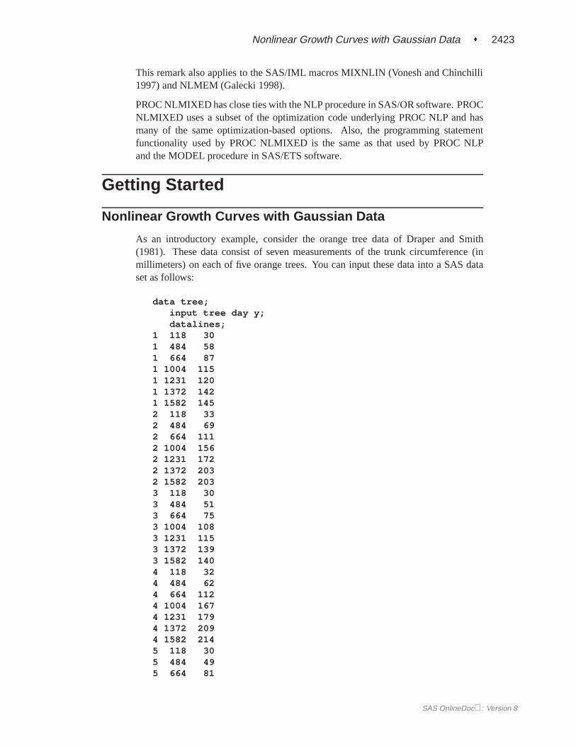
Nonlinear Growth Curves with Gaussian Data
As an introductory example, consider the orange tree data of Draper and Smith(1981). These data consist of seven measurements of the trunk circumference (inmillimeters) on each of five orange trees. You can input these data into a SAS dataset as follows:
data tree;input tree day y;datalines;
1 118 301 484 581 664 871 1004 1151 1231 1201 1372 1421 1582 1452 118 332 484 692 664 1112 1004 1562 1231 1722 1372 2032 1582 2033 118 303 484 513 664 753 1004 1083 1231 1153 1372 1393 1582 1404 118 324 484 624 664 1124 1004 1674 1231 1794 1372 2094 1582 2145 118 305 484 495 664 81
SAS OnlineDoc: Version 8

2424 � Chapter 46. The NLMIXED Procedure
5 1004 1255 1231 1425 1372 1745 1582 177;
Lindstrom and Bates (1990) and Pinheiro and Bates (1995) propose the followinglogistic nonlinear mixed model for these data:
yij =b1 + ui1
1 + exp[�(dij � b2)=b3]+ eij
Here,yij represents thejth measurement on theith tree (i = 1; : : : ; 5; j = 1; : : : ; 7),dij is the corresponding day,b1; b2; b3 are the fixed-effects parameters,ui1 are therandom-effect parameters assumed to be iidN(0; �2u), andeij are the residual errorsassumed to be iidN(0; �2e ) and independent of theui1. This model has a logisticform, and the random-effect parametersui1 enter the model linearly.
The statements to fit this nonlinear mixed model are as follows:
proc nlmixed data=tree;parms b1=190 b2=700 b3=350 s2u=1000 s2e=60;num = b1+u1;ex = exp(-(day-b2)/b3);den = 1 + ex;model y ~ normal(num/den,s2e);random u1 ~ normal(0,s2u) subject=tree;
run;
The PROC NLMIXED statement invokes the procedure and inputs the TREE dataset. The PARMS statement identifies the unknown parameters and their starting val-ues. Here there are three fixed-effects parameters (B1, B2, B3) and two variancecomponents (S2U, S2E).
The next three statements are SAS programming statements specifying the logisticmixed model. A new variable U1 is included to identify the random effect. Thesestatements are evaluated for every observation in the data set when PROC NLMIXEDcomputes the log likelihood function and its derivatives.
The MODEL statement defines the dependent variable and its conditional distribu-tion given the random effects. Here a normal (Gaussian) conditional distribution isspecified with mean NUM/DEN and variance S2E.
The RANDOM statement defines the single random effect to be U1, and specifiesthat it follows a normal distribution with mean 0 and variance S2U. The SUBJECT=argument defines a variable indicating when the random effect obtains new realiza-tions; in this case, it changes according to the values of the TREE variable. PROCNLMIXED assumes that the input data set is clustered according to the levels of theTREE variable; that is, all observations from the same tree occur sequentially in theinput data set.
The output from this analysis is as follows.
SAS OnlineDoc: Version 8

Nonlinear Growth Curves with Gaussian Data � 2425
The NLMIXED Procedure
Specifications
Description Value
Data Set WORK.TREEDependent Variable yDistribution for Dependent Variable NormalRandom Effects u1Distribution for Random Effects NormalSubject Variable treeOptimization Technique Dual Quasi-NewtonIntegration Method Adaptive Gaussian
Quadrature
The “Specifications” table lists some basic information about the nonlinear mixedmodel you have specified. Included are the input data set, dependent and subjectvariables, random effects, relevant distributions, and type of optimization.
The NLMIXED Procedure
Dimensions
Description Value
Observations Used 35Observations Not Used 0Total Observations 35Subjects 5Max Obs Per Subject 7Parameters 5Quadrature Points 1
The “Dimensions” table lists various counts related to the model, including the num-ber of observations, subjects, and parameters. These quantities are useful for check-ing that you have specified your data set and model correctly. Also listed is the num-ber of quadrature points that PROC NLMIXED has selected based on the evaluationof the log likelihood at the starting values of the parameters. Here, only one quadra-ture point is necessary because the random-effect parametersui1 enter the modellinearly.
The NLMIXED Procedure
Parameters
b1 b2 b3 s2u s2e NegLogLike
190 700 350 1000 60 132.491787
SAS OnlineDoc: Version 8

2426 � Chapter 46. The NLMIXED Procedure
The “Parameters” table lists the parameters to be estimated, their starting values, andthe negative log likelihood evaluated at the starting values.
The NLMIXED Procedure
Iteration History
Iter Calls NegLogLike Diff MaxGrad Slope
1 4 131.686742 0.805045 0.010269 -0.6332 6 131.64466 0.042082 0.014783 -0.01823 8 131.614077 0.030583 0.009809 -0.027964 10 131.572522 0.041555 0.001186 -0.013445 11 131.571895 0.000627 0.0002 -0.001216 13 131.571889 5.549E-6 0.000092 -7.68E-67 15 131.571888 1.096E-6 6.097E-6 -1.29E-6
NOTE: GCONV convergence criterion satisfied.
The “Iterations” table records the history of the minimization of the negative log like-lihood. For each iteration of the quasi-Newton optimization, values are listed for thenumber of function calls, the value of the negative log likelihood, the difference fromthe previous iteration, the absolute value of the largest gradient, and the slope of thesearch direction. The note at the bottom of the table indicates that the algorithm hasconverged successfully according to the GCONV convergence criterion, a standardcriterion computed using a quadratic form in the gradient and inverse Hessian.
The NLMIXED Procedure
Fit Statistics
Description Value
-2 Log Likelihood 263.1AIC (smaller is better) 273.1BIC (smaller is better) 271.2Log Likelihood -131.6AIC (larger is better) -136.6BIC (larger is better) -135.6
The“Fitting Information” table lists the final maximized value of the log likelihood aswell as the information criteria of Akaike and Schwarz in two different forms. Thesestatistics can be used to compare different nonlinear mixed models.
SAS OnlineDoc: Version 8
Logistic-Normal Model with Binomial Data � 2427
The NLMIXED Procedure
Parameter Estimates
StandardParameter Estimate Error DF t Value Pr > |t| Alpha Lower
b1 192.05 15.6473 4 12.27 0.0003 0.05 148.61b2 727.90 35.2472 4 20.65 <.0001 0.05 630.04b3 348.07 27.0790 4 12.85 0.0002 0.05 272.88s2u 999.88 647.44 4 1.54 0.1974 0.05 -797.70s2e 61.5139 15.8831 4 3.87 0.0179 0.05 17.4153
Parameter Estimates
Parameter Upper Gradient
b1 235.50 1.154E-6b2 825.76 5.289E-6b3 423.25 -6.1E-6s2u 2797.45 -3.84E-6s2e 105.61 2.892E-6
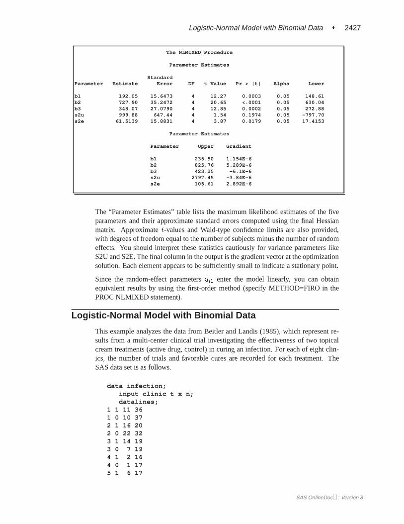
The “Parameter Estimates” table lists the maximum likelihood estimates of the fiveparameters and their approximate standard errors computed using the final Hessianmatrix. Approximatet-values and Wald-type confidence limits are also provided,with degrees of freedom equal to the number of subjects minus the number of randomeffects. You should interpret these statistics cautiously for variance parameters likeS2U and S2E. The final column in the output is the gradient vector at the optimizationsolution. Each element appears to be sufficiently small to indicate a stationary point.
Since the random-effect parametersui1 enter the model linearly, you can obtainequivalent results by using the first-order method (specify METHOD=FIRO in thePROC NLMIXED statement).
Logistic-Normal Model with Binomial Data
This example analyzes the data from Beitler and Landis (1985), which represent re-sults from a multi-center clinical trial investigating the effectiveness of two topicalcream treatments (active drug, control) in curing an infection. For each of eight clin-ics, the number of trials and favorable cures are recorded for each treatment. TheSAS data set is as follows.
data infection;input clinic t x n;datalines;
1 1 11 361 0 10 372 1 16 202 0 22 323 1 14 193 0 7 194 1 2 164 0 1 175 1 6 17
SAS OnlineDoc: Version 8
2428 � Chapter 46. The NLMIXED Procedure
5 0 0 126 1 1 116 0 0 107 1 1 57 0 1 98 1 4 68 0 6 7run;
Supposenij denotes the number of trials for theith clinic and thejth treatment(i = 1; : : : ; 8 j = 0; 1), andxij denotes the corresponding number of favorablecures. Then a reasonable model for the preceding data is the following logistic modelwith random effects:
xij jui � Binomial(nij ; pij)
and
�ij = log
�pij
(1� pij)
�= �0 + �1tj + ui
The notationtj indicates thejth treatment, and theui are assumed to be iidN(0; �2u).
The PROC NLMIXED statements to fit this model are as follows:
proc nlmixed data=infection;parms beta0=-1 beta1=1 s2u=2;eta = beta0 + beta1*t + u;expeta = exp(eta);p = expeta/(1+expeta);model x ~ binomial(n,p);random u ~ normal(0,s2u) subject=clinic;predict eta out=eta;estimate ’1/beta1’ 1/beta1;
run;
The PROC NLMIXED statement invokes the procedure, and the PARMS statementdefines the parameters and their starting values. The next three statements definepij,and the MODEL statement defines the conditional distribution ofxij to be binomial.The RANDOM statement defines U to be the random effect with subjects defined bythe CLINIC variable.
The PREDICT statement constructs predictions for each observation in the input dataset. For this example, predictions of�ij and approximate standard errors of predictionare output to a SAS data set named ETA. These predictions include empirical Bayesestimates of the random effectsui.
The ESTIMATE statement requests an estimate of the reciprocal of�1.
The output for this model is as follows.
SAS OnlineDoc: Version 8

Logistic-Normal Model with Binomial Data � 2429
The NLMIXED Procedure
Specifications
Description Value
Data Set WORK.INFECTIONDependent Variable xDistribution for Dependent Variable BinomialRandom Effects uDistribution for Random Effects NormalSubject Variable clinicOptimization Technique Dual Quasi-NewtonIntegration Method Adaptive Gaussian
Quadrature
The “Specifications” table provides basic information about the nonlinear mixedmodel.
The NLMIXED Procedure
Dimensions
Description Value
Observations Used 16Observations Not Used 0Total Observations 16Subjects 8Max Obs Per Subject 2Parameters 3Quadrature Points 5
The “Dimensions” table provides counts of various variables. You should checkthis table to make sure the data set and model have been entered properly. PROCNLMIXED selects five quadrature points to achieve the default accuracy in the like-lihood calculations.
The NLMIXED Procedure
Parameters
beta0 beta1 s2u NegLogLike
-1 1 2 37.5945925
The “Parameters” table lists the starting point of the optimization.
SAS OnlineDoc: Version 8
2430 � Chapter 46. The NLMIXED Procedure
The NLMIXED Procedure
Iteration History
Iter Calls NegLogLike Diff MaxGrad Slope
1 2 37.3622692 0.232323 2.882077 -19.37622 3 37.1460375 0.216232 0.921926 -0.828523 5 37.0300936 0.115944 0.315897 -0.591754 6 37.0223017 0.007792 0.01906 -0.016155 7 37.0222472 0.000054 0.001743 -0.000116 9 37.0222466 6.57E-7 0.000091 -1.28E-67 11 37.0222466 5.38E-10 2.078E-6 -1.1E-9
NOTE: GCONV convergence criterion satisfied.
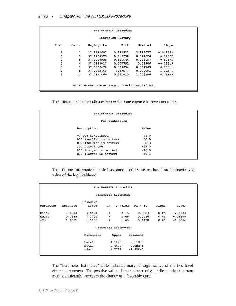
The “Iterations” table indicates successful convergence in seven iterations.
The NLMIXED Procedure
Fit Statistics
Description Value
-2 Log Likelihood 74.0AIC (smaller is better) 80.0BIC (smaller is better) 80.3Log Likelihood -37.0AIC (larger is better) -40.0BIC (larger is better) -40.1
The “Fitting Information” table lists some useful statistics based on the maximizedvalue of the log likelihood.
The NLMIXED Procedure
Parameter Estimates
StandardParameter Estimate Error DF t Value Pr > |t| Alpha Lower
beta0 -1.1974 0.5561 7 -2.15 0.0683 0.05 -2.5123beta1 0.7385 0.3004 7 2.46 0.0436 0.05 0.02806s2u 1.9591 1.1903 7 1.65 0.1438 0.05 -0.8554
Parameter Estimates
Parameter Upper Gradient
beta0 0.1175 -3.1E-7beta1 1.4488 -2.08E-6s2u 4.7736 -2.48E-7
The “Parameter Estimates” table indicates marginal significance of the two fixed-effects parameters. The positive value of the estimate of�1 indicates that the treat-ment significantly increases the chance of a favorable cure.
SAS OnlineDoc: Version 8
Syntax � 2431
The NLMIXED Procedure
Additional Estimates
StandardLabel Estimate Error DF t Value Pr > |t| Alpha Lower Upper
1/beta1 1.3542 0.5509 7 2.46 0.0436 0.05 0.05146 2.6569
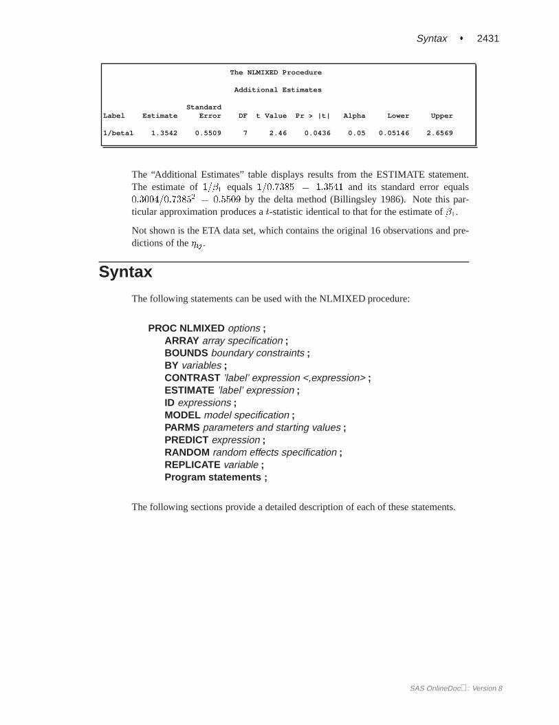
The “Additional Estimates” table displays results from the ESTIMATE statement.The estimate of1=�1 equals1=0:7385 = 1:3541 and its standard error equals0:3004=0:73852 = 0:5509 by the delta method (Billingsley 1986). Note this par-ticular approximation produces at-statistic identical to that for the estimate of�1.
Not shown is the ETA data set, which contains the original 16 observations and pre-dictions of the�ij .
Syntax
The following statements can be used with the NLMIXED procedure:
PROC NLMIXED options ;ARRAY array specification ;BOUNDS boundary constraints ;BY variables ;CONTRAST ’label’ expression <,expression> ;ESTIMATE ’label’ expression ;ID expressions ;MODEL model specification ;PARMS parameters and starting values ;PREDICT expression ;RANDOM random effects specification ;REPLICATE variable ;Program statements ;
The following sections provide a detailed description of each of these statements.
SAS OnlineDoc: Version 8

2432 � Chapter 46. The NLMIXED Procedure
PROC NLMIXED Statement
PROC NLMIXED options ;
This statement invokes the NLMIXED procedure. A large number of options areavailable in the PROC NLMIXED statement, and the following table categorizesthem according to function.
Table 46.1. PROC NLMIXED statement options
Option DescriptionBasic OptionsDATA= input data setMETHOD= integration method
Displayed Output SpecificationsSTART gradient at starting valuesHESS Hessian matrixITDETAILS iteration detailsCORR correlation matrixCOV covariance matrixECORR corr matrix of additional estimatesECOV cov matrix of additional estimatesEDER derivatives of additional estimatesALPHA= alpha for confidence limitsDF= degrees of freedom forp values and confidence limits
Debugging OutputLIST model program, variablesLISTCODE compiled model programLISTDEP model dependency listingLISTDER model derivativeXREF model cross referenceFLOW model execution messagesTRACE detailed model execution messages
Quadrature OptionsNOAD no adaptive centeringNOADSCALE no adaptive scalingOUTQ= output data setQFAC= search factorQMAX= maximum pointsQPOINTS= number of pointsQSCALEFAC= scale factorQTOL= tolerance
Empirical Bayes OptionsEBSTEPS= number of Newton stepsEBSUBSTEPS= number of substepsEBSSFRAC= step-shortening fraction
SAS OnlineDoc: Version 8

PROC NLMIXED Statement � 2433
Table 46.1. (continued)
Option Description
EBSSTOL= step-shortening toleranceEBTOL= convergence toleranceEBOPT comprehensive optimizationEBZSTART zero starting values
Optimization SpecificationsTECHNIQUE= minimization techniqueUPDATE= update techniqueLINESEARCH= line-search methodLSPRECISION= line-search precisionHESCAL= type of Hessian scalingINHESSIAN= start for approximated HessianRESTART= iteration number for update restartOPTCHECK[=] check optimality in neighborhood
Derivatives SpecificationsFD[=] finite-difference derivativesFDHESSIAN[=] finite-difference second derivativesDIAHES use only diagonal of Hessian
Constraint SpecificationsLCEPSILON= range for active constraintsLCDEACT= LM tolerance for deactivatingLCSINGULAR= tolerance for dependent constraints
Termination Criteria SpecificationsMAXFUNC= maximum number of function callsMAXITER= maximum number of iterationsMINITER= minimum number of iterationsMAXTIME= upper limit seconds of CPU timeABSCONV= absolute function convergence criterionABSFCONV= absolute function convergence criterionABSGCONV= absolute gradient convergence criterionABSXCONV= absolute parameter convergence criterionFCONV= relative function convergence criterionFCONV2= relative function convergence criterionGCONV= relative gradient convergence criterionXCONV= relative parameter convergence criterionFDIGITS= number accurate digits in objective functionFSIZE= used in FCONV, GCONV criterionXSIZE= used in XCONV criterion
Step Length SpecificationsDAMPSTEP[=] damped steps in line searchMAXSTEP= maximum trust-region radiusINSTEP= initial trust-region radius
SAS OnlineDoc: Version 8

2434 � Chapter 46. The NLMIXED Procedure
Table 46.1. (continued)
Option Description
Singularity TolerancesSINGCHOL= tolerance for Cholesky rootsSINGHESS= tolerance for HessianSINGSWEEP= tolerance for sweepSINGVAR= tolerance for variances
Covariance Matrix TolerancesASINGULAR= absolute singularity for inertiaMSINGULAR= relative M singularity for inertiaVSINGULAR= relative V singularity for inertiaG4= threshold for Moore-Penrose inverseCOVSING= tolerance for singular COV matrixCFACTOR= multiplication factor for COV matrix
These options are described in alphabetical order. For a description of the mathemat-ical notation used in the following sections, see the section “Modeling Assumptionsand Notation.”
ABSCONV=rABSTOL= r
specifies an absolute function convergence criterion. For minimization, terminationrequiresf(�(k)) � r: The default value ofr is the negative square root of the largestdouble precision value, which serves only as a protection against overflows.
ABSFCONV=r[n]ABSFTOL= r[n]
specifies an absolute function convergence criterion. For all techniques exceptNMSIMP, termination requires a small change of the function value in successiveiterations:
jf(�(k�1))� f(�(k))j � r
The same formula is used for the NMSIMP technique, but�(k) is defined as the vertexwith the lowest function value, and�(k�1) is defined as the vertex with the highestfunction value in the simplex. The default value isr = 0. The optional integervaluen specifies the number of successive iterations for which the criterion must besatisfied before the process can be terminated.
ABSGCONV=r[n]ABSGTOL= r[n]
specifies an absolute gradient convergence criterion. Termination requires the maxi-mum absolute gradient element to be small:
maxjjgj(�(k))j � r
This criterion is not used by the NMSIMP technique. The default value isr = 1E�5.The optional integer valuen specifies the number of successive iterations for whichthe criterion must be satisfied before the process can be terminated.
SAS OnlineDoc: Version 8

PROC NLMIXED Statement � 2435
ABSXCONV=r[n]ABSXTOL= r[n]
specifies an absolute parameter convergence criterion. For all techniques exceptNMSIMP, termination requires a small Euclidean distance between successive pa-rameter vectors,
k �(k) � �(k�1) k2� r
For the NMSIMP technique, termination requires either a small length�(k) of thevertices of a restart simplex,
�(k) � r
or a small simplex size,�(k) � r
where the simplex size�(k) is defined as the L1 distance from the simplex vertex�(k)
with the smallest function value to the othern simplex points�(k)l 6= �(k):
�(k) =X�l 6=y
k �(k)l � �(k) k1
The default isr = 1E � 8 for the NMSIMP technique andr = 0 otherwise. Theoptional integer valuen specifies the number of successive iterations for which thecriterion must be satisfied before the process can terminate.
ALPHA=�specifies the alpha level to be used in computing confidence limits. The default valueis 0.05.
ASINGULAR= rASING=r
specifies an absolute singularity criterion for the computation of the inertia (numberof positive, negative, and zero eigenvalues) of the Hessian and its projected forms.The default value is the square root of the smallest positive double precision value.
CFACTOR=fspecifies a multiplication factorf for the estimated covariance matrix of the parame-ter estimates.
COVrequests the approximate covariance matrix for the parameter estimates.
CORRrequests the approximate correlation matrix for the parameter estimates.
COVSING=r > 0specifies a nonnegative threshold that determines whether the eigenvalues of a singu-lar Hessian matrix are considered to be zero.
DAMPSTEP[= r]DS[= r]
specifies that the initial step-size value�(0) for each line search (used by theQUANEW, CONGRA, or NEWRAP technique) cannot be larger thanr times the
SAS OnlineDoc: Version 8

2436 � Chapter 46. The NLMIXED Procedure
step-size value used in the former iteration. If you specify the DAMPSTEP optionwithout factorr, the default value isr = 2. The DAMPSTEP=r option can pre-vent the line-search algorithm from repeatedly stepping into regions where some ob-jective functions are difficult to compute or where they could lead to floating pointoverflows during the computation of objective functions and their derivatives. TheDAMPSTEP=r option can save time-costly function calls that result in very smallstep sizes�. For more details on setting the start values of each line search, see thesection “Restricting the Step Length,” beginning on page 2471.
DATA=SAS-data-setspecifies the input data set. Observations in this data set are used to compute the loglikelihood function that you specify with PROC NLMIXED statements.
NOTE: If you are using a RANDOM statement, the input data set must be clus-tered according to the SUBJECT= variable. One easy way to accomplish this is tosort your data by the SUBJECT= variable prior to calling PROC NLMIXED. PROCNLMIXED does not sort the input data set for you.
DF=dspecifies the degrees of freedom to be used in computingp values and confidencelimits. The default value is the number of subjects minus the number of randomeffects for random effects models, and the number of observations otherwise.
DIAHESspecifies that only the diagonal of the Hessian is used.
EBOPTrequests that a more comprehensive optimization be carried out if the default empiri-cal Bayes optimization fails to converge.
EBSSFRAC=r > 0specifies the step-shortening fraction to be used while computing empirical Bayesestimates of the random effects. The default value is 0.8.
EBSSTOL=r � 0specifies the objective function tolerance for determining the cessation of step-shortening while computing empirical Bayes estimates of the random effects. Thedefault value isr = 1E� 8.
EBSTEPS=n � 0specifies the maximum number of Newton steps for computing empirical Bayes esti-mates of random effects. The default value isn = 50.
EBSUBSTEPS=n � 0specifies the maximum number of step-shortenings for computing empirical Bayesestimates of random effects. The default value isn = 20.
EBTOL=r � 0specifies the convergence tolerance for empirical Bayes estimation. The default valueis r = �E4, where� is the machine precision. This default value equals approximately1E� 12 on most machines.
SAS OnlineDoc: Version 8

PROC NLMIXED Statement � 2437
EBZSTARTrequests that a zero be used as starting values during empirical Bayes estimation. Bydefault, the starting values are set equal to the estimates from the previous iteration(or zero for the first iteration).
ECOVrequests the approximate covariance matrix for all expressions specified in ESTI-MATE statements.
ECORRrequests the approximate correlation matrix for all expressions specified in ESTI-MATE statements.
EDERrequests the derivatives of all expressions specified in ESTIMATE statements withrespect to each of the model parameters.
FCONV=r[n]FTOL=r[n]
specifies a relative function convergence criterion. For all techniques exceptNMSIMP, termination requires a small relative change of the function value in suc-cessive iterations,
jf(�(k))� f(�(k�1))jmax(jf(�(k�1))j;FSIZE)
� r
where FSIZE is defined by the FSIZE= option. The same formula is used for theNMSIMP technique, but�(k) is defined as the vertex with the lowest function value,and�(k�1) is defined as the vertex with the highest function value in the simplex.The default isr=10�FDIGITSwhere FDIGITS is the value of the FDIGITS= option.The optional integer valuen specifies the number of successive iterations for whichthe criterion must be satisfied before the process can terminate.
FCONV2=r[n]FTOL2=r[n]
specifies another function convergence criterion. For all techniques except NMSIMP,termination requires a small predicted reduction
df (k) � f(�(k))� f(�(k) + s(k))
of the objective function. The predicted reduction
df (k) = �g(k)T s(k) � 1
2s(k)TH(k)s(k)
= �1
2s(k)T g(k)
� r
is computed by approximating the objective functionf by the first two terms of theTaylor series and substituting the Newton step.
s(k) = �[H(k)]�1g(k)
SAS OnlineDoc: Version 8

2438 � Chapter 46. The NLMIXED Procedure
For the NMSIMP technique, termination requires a small standard deviation of the
function values of then+ 1 simplex vertices�(k)l , l = 0; : : : ; n,s1
n+ 1
Xl
hf(�
(k)l )� f(�(k))
i2 � r
wheref(�(k)) = 1n+1
Pl f(�
(k)l ). If there arenact boundary constraints active at
�(k), the mean and standard deviation are computed only for then + 1 � nact un-constrained vertices. The default value isr = 1E � 6 for the NMSIMP techniqueandr = 0 otherwise. The optional integer valuen specifies the number of successiveiterations for which the criterion must be satisfied before the process can terminate.
FD[= FORWARD | CENTRAL | r]specifies that all derivatives be computed using finite difference approximations. Thefollowing specifications are permitted:
FD is equivalent to FD=100.
FD=CENTRAL uses central differences.
FD=FORWARD uses forward differences.
FD=r uses central differences for the initial and final evaluations of thegradient, and Hessian. During iteration, start with forward dif-ferences and switch to a corresponding central-difference formuladuring the iteration process when one of the following two criteriais satisfied:
� The absolute maximum gradient element is less than or equalto r times the ABSGTOL threshold.
� The normalized predicted function reduction (see theGTOL option on page 2439) is less than or equal tomax(1E� 6; r �GTOL). The 1E � 6 ensures that theswitch is done, even if you set the GTOL threshold to zero.
Note that the FD and FDHESSIAN options cannot apply at the same time. TheFDHESSIAN option is ignored when only first-order derivatives are used. See thesection “Finite Difference Approximations of Derivatives,” beginning on page 2465,for more information.
FDHESSIAN[= FORWARD | CENTRAL]FDHES[= FORWARD | CENTRAL]FDH[= FORWARD | CENTRAL]
specifies that second-order derivatives be computed using finite difference approxi-mations based on evaluations of the gradients.
FDHESSIAN=FORWARD uses forward differences.
FDHESSIAN=CENTRAL uses central differences.
FDHESSIAN uses forward differences for the Hessian except for the initial andfinal output.
SAS OnlineDoc: Version 8

PROC NLMIXED Statement � 2439
Note that the FD and FDHESSIAN options cannot apply at the same time. See thesection “Finite Difference Approximations of Derivatives,” beginning on page 2465,for more information.
FDIGITS=rspecifies the number of accurate digits in evaluations of the objective function. Frac-tional values such as FDIGITS=4.7 are allowed. The default value isr = � log10 �,where� is the machine precision. The value ofr is used to compute the interval sizeh for the computation of finite-difference approximations of the derivatives of theobjective function and for the default value of the FCONV= option.
FLOWdisplays a message for each statement in the model program as it is executed. Thisdebugging option is very rarely needed and produces voluminous output.
FSIZE=rspecifies the FSIZE parameter of the relative function and relative gradient termina-tion criteria. The default value isr = 0. For more details, see the FCONV= andGCONV= options.
G4=n > 0specifies a dimension to determine the type of generalized inverse to use when theapproximate covariance matrix of the parameter estimates is singular. The defaultvalue ofn is 60. See the section “Covariance Matrix,” beginning on page 2475, formore information.
GCONV=r[n]GTOL=r[n]
specifies a relative gradient convergence criterion. For all techniques except CON-GRA and NMSIMP, termination requires that the normalized predicted function re-duction is small,
g(�(k))T [H(k)]�1g(�(k))
max(jf(�(k))j;FSIZE)� r
where FSIZE is defined by the FSIZE= option. For the CONGRA technique (wherea reliable Hessian estimateH is not available), the following criterion is used:
k g(�(k)) k22 k s(�(k)) k2k g(�(k))� g(�(k�1)) k2 max(jf(�(k))j;FSIZE)
� r
This criterion is not used by the NMSIMP technique. The default value isr =1E�8. The optional integer valuen specifies the number of successive iterations forwhich the criterion must be satisfied before the process can terminate.
HESCAL=0j1j2j3HS=0j1j2j3
specifies the scaling version of the Hessian matrix used in NRRIDG, TRUREG,NEWRAP, or DBLDOG optimization. If HS is not equal to 0, the first iteration
and each restart iteration sets the diagonal scaling matrixD(0) = diag(d(0)i ):
d(0)i =
qmax(jH(0)
i;i j; �)
SAS OnlineDoc: Version 8

2440 � Chapter 46. The NLMIXED Procedure
whereH(0)i;i are the diagonal elements of the Hessian. In every other iteration, the
diagonal scaling matrixD(0) = diag(d(0)i ) is updated depending on the HS op-
tion:
HS=0 specifies that no scaling is done.
HS=1 specifies the Moré (1978) scaling update:
d(k+1)i = max
�d(k)i ;
qmax(jH(k)
i;i j; �)�
HS=2 specifies the Dennis, Gay, & Welsch (1981) scaling update:
d(k+1)i = max
�0:6 � d(k)i ;
qmax(jH(k)
i;i j; �)�
HS=3 specifies thatdi is reset in each iteration:
d(k+1)i =
qmax(jH(k)
i;i j; �)
In each scaling update,� is the relative machine precision. The default value is HS=0.Scaling of the Hessian can be time consuming in the case where general linear con-straints are active.
HESSrequests the display of the final Hessian matrix after optimization. If you also specifythe START option, then the Hessian at the starting values is also printed.
INHESSIAN[= r]INHESS[= r]
specifies how the initial estimate of the approximate Hessian is defined for the quasi-Newton techniques QUANEW and DBLDOG. There are two alternatives:
� If you do not use ther specification, the initial estimate of the approximateHessian is set to the Hessian at�(0).
� If you do use ther specification, the initial estimate of the approximate Hessianis set to the multiple of the identity matrixrI.
By default, if you do not specify the option INHESSIAN=r, the initial estimate of theapproximate Hessian is set to the multiple of the identity matrixrI, where the scalarr is computed from the magnitude of the initial gradient.
INSTEP=rreduces the length of the first trial step during the line search of the first iterations.For highly nonlinear objective functions, such as the EXP function, the default ini-tial radius of the trust-region algorithm TRUREG or DBLDOG or the default steplength of the line-search algorithms can result in arithmetic overflows. If this oc-curs, you should specify decreasing values of0 < r < 1 such as INSTEP=1E � 1,INSTEP=1E� 2, INSTEP=1E� 4, and so on, until the iteration starts successfully.
SAS OnlineDoc: Version 8

PROC NLMIXED Statement � 2441
� For trust-region algorithms (TRUREG, DBLDOG), the INSTEP= option spec-ifies a factorr > 0 for the initial radius�(0) of the trust region. The defaultinitial trust-region radius is the length of the scaled gradient. This step corre-sponds to the default radius factor ofr = 1.
� For line-search algorithms (NEWRAP, CONGRA, QUANEW), the INSTEP=option specifies an upper bound for the initial step length for the line searchduring the first five iterations. The default initial step length isr = 1.
� For the Nelder-Mead simplex algorithm, using TECH=NMSIMP, theINSTEP=r option defines the size of the start simplex.
For more details, see the section “Computational Problems,” beginning onpage 2472.
ITDETAILS=requests a more complete iteration history, including the current values of the pa-rameter estimates, their gradients, and additional optimization statistics. For furtherdetails, see the section “Iterations” beginning on page 2479.
LCDEACT=rLCD=r
specifies a thresholdr for the Lagrange multiplier that determines whether an activeinequality constraint remains active or can be deactivated. During minimization, anactive inequality constraint can be deactivated only if its Lagrange multiplier is lessthan the threshold valuer < 0. The default value is
r = �min(0:01;max(0:1 �ABSGCONV; 0:001 � gmax(k)))
where ABSGCONV is the value of the absolute gradient criterion, andgmax(k) isthe maximum absolute element of the (projected) gradientg(k) or ZT g(k). (See thesection “Active Set Methods,” beginning on page 2468, for a definition ofZ.)
LCEPSILON=r > 0LCEPS=r > 0LCE=r > 0
specifies the range for active and violated boundary constraints. The default value isr = 1E�8. During the optimization process, the introduction of rounding errors canforce PROC NLMIXED to increase the value ofr by a factor of10; 100; : : :. If thishappens, it is indicated by a message displayed in the log.
LCSINGULAR= r > 0LCSING=r > 0LCS=r > 0
specifies a criterionr, used in the update of the QR decomposition, that determineswhether an active constraint is linearly dependent on a set of other active constraints.The default value isr = 1E�8. The largerr becomes, the more the active constraintsare recognized as being linearly dependent. If the value ofr is larger than0:1, it isreset to0:1.
SAS OnlineDoc: Version 8

2442 � Chapter 46. The NLMIXED Procedure
LINESEARCH=iLIS=i
specifies the line-search method for the CONGRA, QUANEW, and NEWRAP opti-mization techniques. Refer to Fletcher (1987) for an introduction to line-search tech-niques. The value ofi can be1; : : : ; 8. For CONGRA, QUANEW and NEWRAP,the default value isi = 2.
LIS=1 specifies a line-search method that needs the same number of func-tion and gradient calls for cubic interpolation and cubic extrapola-tion; this method is similar to one used by the Harwell subroutinelibrary.
LIS=2 specifies a line-search method that needs more function than gra-dient calls for quadratic and cubic interpolation and cubic ex-trapolation; this method is implemented as shown in Fletcher(1987) and can be modified to an exact line search by using theLSPRECISION= option.
LIS=3 specifies a line-search method that needs the same number offunction and gradient calls for cubic interpolation and cubic ex-trapolation; this method is implemented as shown in Fletcher(1987) and can be modified to an exact line search by using theLSPRECISION= option.
LIS=4 specifies a line-search method that needs the same number of func-tion and gradient calls for stepwise extrapolation and cubic inter-polation.
LIS=5 specifies a line-search method that is a modified version of LIS=4.
LIS=6 specifies golden section line search (Polak 1971), which uses onlyfunction values for linear approximation.
LIS=7 specifies bisection line search (Polak 1971), which uses only func-tion values for linear approximation.
LIS=8 specifies the Armijo line-search technique (Polak 1971), whichuses only function values for linear approximation.
LISTdisplays the model program and variable lists. The LIST option is a debugging featureand is not normally needed.
LISTCODEdisplays the derivative tables and the compiled program code. The LISTCODE optionis a debugging feature and is not normally needed.
LSPRECISION=rLSP=r
specifies the degree of accuracy that should be obtained by the line-search algorithmsLIS=2 and LIS=3. Usually an imprecise line search is inexpensive and successful.For more difficult optimization problems, a more precise and expensive line searchmay be necessary (Fletcher 1987). The second line-search method (which is the
SAS OnlineDoc: Version 8

PROC NLMIXED Statement � 2443
default for the NEWRAP, QUANEW, and CONGRA techniques) and the third line-search method approach exact line search for small LSPRECISION= values. If youhave numerical problems, you should try to decrease the LSPRECISION= value toobtain a more precise line search. The default values are shown in the following table.
TECH= UPDATE= LSP defaultQUANEW DBFGS, BFGS r = 0.4QUANEW DDFP, DFP r = 0.06CONGRA all r = 0.1NEWRAP no update r = 0.9
For more details, refer to Fletcher (1987).
MAXFUNC=iMAXFU=i
specifies the maximum numberi of function calls in the optimization process. Thedefault values are
� TRUREG, NRRIDG, NEWRAP: 125
� QUANEW, DBLDOG: 500
� CONGRA: 1000
� NMSIMP: 3000
Note that the optimization can terminate only after completing a full iteration. There-fore, the number of function calls that is actually performed can exceed the numberthat is specified by the MAXFUNC= option.
MAXITER=iMAXIT=i
specifies the maximum numberi of iterations in the optimization process. The defaultvalues are
� TRUREG, NRRIDG, NEWRAP: 50
� QUANEW, DBLDOG: 200
� CONGRA: 400
� NMSIMP: 1000
These default values are also valid wheni is specified as a missing value.
MAXSTEP=r[n]specifies an upper bound for the step length of the line-search algorithms during thefirstn iterations. By default,r is the largest double precision value andn is the largestinteger available. Setting this option can improve the speed of convergence for theCONGRA, QUANEW, and NEWRAP techniques.
MAXTIME=rspecifies an upper limit ofr seconds of CPU time for the optimization process. Thedefault value is the largest floating point double representation of your computer.Note that the time specified by the MAXTIME= option is checked only once at the
SAS OnlineDoc: Version 8

2444 � Chapter 46. The NLMIXED Procedure
end of each iteration. Therefore, the actual running time can be much longer thanthat specified by the MAXTIME= option. The actual running time includes the restof the time needed to finish the iteration and the time needed to generate the outputof the results.
METHOD=valuespecifies the method for approximating the integral of the likelihood over the randomeffects. Valid values are as follows.
� FIROspecifies the first-order method of Beal and Sheiner (1982).
� GAUSSspecifies adaptive Gauss-Hermite quadrature (Pinheiro and Bates 1995). You
can prevent the adaptation with the NOAD option or prevent adaptive scalingwith the NOADSCALE option. This is the default integration method.
� HARDYspecifies Hardy quadrature based on an adaptive trapezoidal rule. This methodis available only for one-dimensional integrals; that is, you must specify onlyone random effect.
� ISAMPspecifies adaptive importance sampling (Pinheiro and Bates 1995) . You can
prevent the adaptation with the NOAD option or prevent adaptive scaling withthe NOADSCALE option. You can use the SEED= option to specify a start-ing seed for the random number generation used in the importance sampling;otherwise, PROC NLMIXED uses the clock time as a seed.
MINITER=iMINIT=i
specifies the minimum number of iterations. The default value is 0. If you requestmore iterations than are actually needed for convergence to a stationary point, theoptimization algorithms can behave strangely. For example, the effect of roundingerrors can prevent the algorithm from continuing for the required number of itera-tions.
MSINGULAR=r > 0MSING=r > 0
specifies a relative singularity criterion for the computation of the inertia (number ofpositive, negative, and zero eigenvalues) of the Hessian and its projected forms. Thedefault value is1E � 12 if you do not specify the SINGHESS= option; otherwise,the default value ismax(10�; 1E � 4 � SINGHESS). See the section “CovarianceMatrix,” beginning on page 2475, for more information.
NOADrequests that the Gaussian quadrature be nonadaptive; that is, the quadrature pointsare centered at zero for each of the random effects and the current random-effectsvariance matrix is used as the scale matrix.
SAS OnlineDoc: Version 8

PROC NLMIXED Statement � 2445
NOADSCALErequests nonadaptive scaling for adaptive Gaussian quadrature; that is, the quadraturepoints are centered at the empirical Bayes estimates for the the random effects, butthe current random-effects variance matrix is used as the scale matrix. By default,the observed Hessian from the current empirical Bayes estimates is used as the scalematrix.
OPTCHECK[= r > 0]computes the function valuesf(�l) of a grid of points�l in a ball of radius ofrabout��. If you specify the OPTCHECK option without factorr, the default valueis r = 0:1 at the starting point andr = 0:01 at the terminating point. If a point��l isfound with a better function value thanf(��), then optimization is restarted at��l .
OUTQ=SAS-data-setspecifies an output data set containing the quadrature points used for numerical inte-gration.
QFAC=r > 0specifies the additive factor used to adaptively search for the number of quadraturepoints. For METHOD=GAUSS, the search sequence is 1, 3, 5, 7, 9, 11, 11 +r,11 + 2r, : : :, where the default value ofr is 10. For METHOD=ISAMP, the searchsequence is 10, 10 +r, 10 +2r, : : :, where the default value ofr is 50.
QMAX=r > 0specifies the maximum number of quadrature points permitted before the adaptivesearch is aborted. The default values are 31 for adaptive Gaussian quadrature, 61 fornon-adaptive Gaussian quadrature, 160 for adaptive importance sampling, and 310for non-adaptive importance sampling.
QPOINTS=n > 0specifies the number of quadrature points to be used during evaluation of integrals.For METHOD=GAUSS,n equals the number of points used in each dimension of therandom effects, resulting in a total ofnr points, wherer is the number of dimensions.For METHOD=ISAMP,n specifies the total number of quadrature points regardlessof the dimension of the random effects. By default, the number of quadrature pointsis selected adaptively, and this option disables the adaptive search.
QSCALEFAC= r > 0specifies a multiplier for the scale matrix used during quadrature calculations. Thedefault value is 1.0.
QTOL=r > 0specifies the tolerance used to adaptively select the number of quadrature points.When the relative difference between two successive likelihood calculations is lessthanr, then the search terminates and the lesser number of quadrature points is usedduring the subsequent optimization process. The default value is1E� 4.
SAS OnlineDoc: Version 8
2446 � Chapter 46. The NLMIXED Procedure
RESTART=i > 0REST=i > 0
specifies that the QUANEW or CONGRA algorithm is restarted with a steepest de-scent/ascent search direction after, at most,i iterations. Default values are
� CONGRA: UPDATE=PB: restart is performed automatically,i is not used.
� CONGRA: UPDATE6=PB: i = min(10n; 80), wheren is the number of pa-rameters.
� QUANEW: i is the largest integer available.
SEED=i > 0specifies the random number seed for METHOD=ISAMP.
SINGCHOL=r > 0specifies the singularity criterionr for Cholesky roots of the random-effects variancematrix and scale matrix for adaptive Gaussian quadrature. The default value is1E4times the machine epsilon; this product is approximately1E�12 on most computers.
SINGHESS=r > 0specifies the singularity criterionr for the inversion of the Hessian matrix. The de-fault value is1E � 8. See the ASINGULAR, MSINGULAR=, and VSINGULAR=options for more information.
SINGSWEEP=r > 0specifies the singularity criterionr for inverting the variance matrix in the first-ordermethod and the empirical Bayes Hessian matrix. The default value is1E4 times themachine epsilon; this product is approximately1E� 12 on most computers.
SINGVAR=r > 0specifies the singularity criterionr below which statistical variances are consideredto equal zero. The default value is1E4 times the machine epsilon; this product isapproximately1E� 12 on most computers.
STARTrequests that the gradient of the log likelihood at the starting values be displayed. Ifyou also specify the HESS option, then the starting Hessian is displayed as well.
TECHNIQUE=valueTECH=value
specifies the optimization technique. Valid values are
� CONGRAperforms a conjugate-gradient optimization, which can be more precisely spec-ified with the UPDATE= option and modified with the LINESEARCH= option.When you specify this option, UPDATE=PB by default.
� DBLDOGperforms a version of double dogleg optimization, which can be more pre-
cisely specified with the UPDATE= option. When you specify this option,UPDATE=DBFGS by default.
� NMSIMPperforms a Nelder-Mead simplex optimization.
SAS OnlineDoc: Version 8

PROC NLMIXED Statement � 2447
� NONEdoes not perform any optimization. This option can be used
– to perform a grid search without optimization
– to compute estimates and predictions that cannot be obtained efficientlywith any of the optimization techniques
� NEWRAPperforms a Newton-Raphson optimization combining a line-search algorithm
with ridging. The line-search algorithm LIS=2 is the default method.
� NRRIDGperforms a Newton-Raphson optimization with ridging.
� QUANEWperforms a quasi-Newton optimization, which can be defined more precisely
with the UPDATE= option and modified with the LINESEARCH= option. Thisis the default estimation method.
� TRUREGperforms a trust region optimization.
TRACEdisplays the result of each operation in each statement in the model program as it isexecuted. This debugging option is very rarely needed, and it produces voluminousoutput.
UPDATE=methodUPD=method
specifies the update method for the quasi-Newton, double dogleg, or conjugate-gradient optimization technique. Not every update method can be used with eachoptimizer. See the section “Optimization Algorithms,” beginning on page 2460, formore information. Valid methods are
� BFGSperforms the original Broyden, Fletcher, Goldfarb, and Shanno (BFGS) updateof the inverse Hessian matrix.
� DBFGSperforms the dual BFGS update of the Cholesky factor of the Hessian matrix.This is the default update method.
� DDFPperforms the dual Davidon, Fletcher, and Powell (DFP) update of the Choleskyfactor of the Hessian matrix.
� DFPperforms the original DFP update of the inverse Hessian matrix.
� PBperforms the automatic restart update method of Powell (1977) and Beale
(1972).
SAS OnlineDoc: Version 8
2448 � Chapter 46. The NLMIXED Procedure
� FRperforms the Fletcher-Reeves update (Fletcher 1987).
� PRperforms the Polak-Ribiere update (Fletcher 1987).
� CDperforms a conjugate-descent update of Fletcher (1987).
VSINGULAR=r > 0VSING=r > 0
specifies a relative singularity criterion for the computation of the inertia (numberof positive, negative, and zero eigenvalues) of the Hessian and its projected forms.The default value isr = 1E � 8 if the SINGHESS= option is not specified, and itis the value of SINGHESS= option otherwise. See the section “Covariance Matrix,”beginning on page 2475, for more information.
XCONV=r[n]XTOL=r[n]
specifies the relative parameter convergence criterion. For all techniques exceptNMSIMP, termination requires a small relative parameter change in subsequent it-erations.
maxj j�(k)j � �(k�1)j j
max(j�(k)j j; j�(k�1)j j;XSIZE)� r
For the NMSIMP technique, the same formula is used, but�(k)j is defined as the
vertex with the lowest function value and�(k�1)j is defined as the vertex with thehighest function value in the simplex. The default value isr = 1E � 8 for theNMSIMP technique andr = 0 otherwise. The optional integer valuen specifies thenumber of successive iterations for which the criterion must be satisfied before theprocess can be terminated.
XSIZE=r > 0specifies the XSIZE parameter of the relative parameter termination criterion. Thedefault value isr = 0. For more detail, see the XCONV= option.
ARRAY Statement
ARRAY arrayname [{ dimensions }] [$] [variables and constants] ;
The ARRAY statement is similar to, but not the same as, the ARRAY statement inthe SAS DATA step, and it is the same as the ARRAY statements in the NLIN, NLP,and MODEL procedures. The ARRAY statement is used to associate a name (of nomore than eight characters) with a list of variables and constants. The array nameis used with subscripts in the program to refer to the array elements. The followingstatements illustrate this.
SAS OnlineDoc: Version 8
BOUNDS Statement � 2449
array r[8] r1-r8;
do i = 1 to 8;r[i] = 0;
end;
The ARRAY statement does not support all the features of the ARRAY statement inthe DATA step. It cannot be used to assign initial values to array elements. Implicitindexing of variables cannot be used; all array references must have explicit subscriptexpressions. Only exact array dimensions are allowed; lower-bound specifications arenot supported. A maximum of six dimensions is allowed.
On the other hand, the ARRAY statement does allow both variables and constants tobe used as array elements. (Constant array elements cannot have values assigned tothem.) Both dimension specification and the list of elements are optional, but at leastone must be specified. When the list of elements is not specified or fewer elementsthan the size of the array are listed, array variables are created by suffixing elementnumbers to the array name to complete the element list.
BOUNDS Statement
BOUNDS b–con [ , b–con... ] ;
where b–con := numberoperatorparameter–list operatornumberor b–con := numberoperatorparameter–listor b–con := parameter–list operatornumber
and operator:= <=, <, >=, or>
Boundary constraints are specified with a BOUNDS statement. One- or two-sidedboundary constraints are allowed. The list of boundary constraints are separated bycommas. For example,
bounds 0 <= a1-a9 X <= 1, -1 <= c2-c5;bounds b1-b10 y >= 0;
You can specify more than one BOUNDS statement. If you specify more than onelower (upper) bound for the same parameter, the maximum (minimum) of these istaken.
If the maximumlj of all lower bounds is larger than the minimum of all upper boundsuj for the same variable�j , the boundary constraint is replaced by�j := lj :=min(uj) defined by the minimum of all upper bounds specified for�j .
SAS OnlineDoc: Version 8

2450 � Chapter 46. The NLMIXED Procedure
BY Statement
BY variables ;
You can use a BY statement with PROC NLMIXED to obtain separate analyses onDATA= data set observations in groups defined by the BY variables. This meansthat, unless TECH=NONE, an optimization problem is solved for each BY groupseparately. When a BY statement appears, the procedure expects the input DATA=data set to be sorted in order of the BY variables. If your input data set is not sortedin ascending order, use one of the following alternatives:
� Use the SORT procedure with a similar BY statement to sort the data.
� Use the BY statement option NOTSORTED or DESCENDING in the BY state-ment for the NLMIXED procedure. As a cautionary note, the NOTSORTEDoption does not mean that the data are unsorted but rather that the data arearranged in groups (according to values of the BY variables) and that thesegroups are not necessarily in alphabetical or increasing numeric order.
� Use the DATASETS procedure (in Base SAS software) to create an index onthe BY variables.
For more information on the BY statement, refer to the discussion inSAS LanguageReference: Concepts. For more information on the DATASETS procedure, refer tothe discussion in theSAS Procedures Guide.
CONTRAST Statement
CONTRAST ’label’ expression <, expression> <options> ;
The CONTRAST statement enables you to conduct a statistical test that several ex-pressions simultaneously equal zero. The expressions are typically contrasts, that is,differences whose expected values equal zero under the hypothesis of interest.
In the CONTRAST statement you must provide a quoted string to identify the con-trast and then a list of valid SAS expressions separated by commas. Multiple CON-TRAST statements are permitted, and results from all statements are listed in a com-mon table. PROC NLMIXED constructs approximateF tests for each statementusing the delta method (Billingsley 1986) to approximate the variance-covariancematrix of the constituent expressions.
The following option is available in the CONTRAST statement.
SAS OnlineDoc: Version 8
ID Statement � 2451
DF=dspecifies the denominator degrees of freedom to be used in computingp values forthe F statistics. The default value corresponds to the DF= option in the PROCNLMIXED statement.
ESTIMATE Statement
ESTIMATE ’label’ expression <options> ;
The ESTIMATE statement enables you to compute an additional estimate that isa function of the parameter values. You must provide a quoted string to identifythe estimate and then a valid SAS expression. Multiple ESTIMATE statements arepermitted, and results from all statements are listed in a common table. PROCNLMIXED computes approximate standard errors for the estimates using the deltamethod (Billingsley 1986). It uses these standard errors to compute correspondingtstatistics,p-values, and confidence limits.
The ECOV option in the PROC NLMIXED statement produces a table containingthe approximate covariance matix of all of the additional estimates you specify. TheECORR option produces the corresponding correlation matrix. The EDER optionproduces a table of the derivatives of the additional estimates with respect to each ofthe model parameters.
The following options are available in the ESTIMATE statement:
ALPHA=�specifies the alpha level to be used in computing confidence limits. The default valuecorresponds to the ALPHA= option in the PROC NLMIXED statement.
DF=dspecifies the degrees of freedom to be used in computingp-values and confidencelimits. The default value corresponds to the DF= option in the PROC NLMIXEDstatement.
ID Statement
ID expressions ;
The ID statement identifies additional quantities to be included in the OUT= data setof the PREDICT statement. These can be any symbols you have defined with SASprogramming statements.
SAS OnlineDoc: Version 8

2452 � Chapter 46. The NLMIXED Procedure
MODEL Statement
MODEL dependent-variable � distribution ;
The MODEL statement is the mechanism for specifying the conditional distributionof the data given the random effects. You must specify a single dependent variablefrom the input data set, a tilde (�), and then a distribution with its parameters. Validdistributions are as follows.
� normal(m,v)specifies a normal (Gaussian) distribution with meanm and vari-ancev.
� binary(p)specifies a binary (Bernouilli) distribution with probabilityp.
� binomial(n,p)specifies a binomial distribution with countn and probabilityp.
� poisson(m)specifies a Poisson distribution with meanm.
� general(ll) specifies a general log likelihood function that you construct usingSAS programming statements.
PARMS Statement
PARMS <name–list [=numbers] [ , name–list [=numbers] ... ]></ options> ;
The PARMS statement lists names of parameters and specifies initial values, possiblyover a grid. You can specify the parameters and values either directly in a list orprovide the name of a SAS data set that contains them using the DATA= option.
While the PARMS statement is not required, you are encouraged to use it to providePROC NLMIXED with accurate starting values. Parameters not listed in the PARMSstatement are assigned an initial value of 1. PROC NLMIXED considers all symbolsnot assigned values to be parameters, so you should specify your modeling statementscarefully and check the output from the “Parameters” table to make sure the properparameters are identified.
A list of parameter names in the PARMS statement is not separated by commas andis followed by an equal sign and a list of numbers. If the number list consists of onlyone number, this number defines the initial value for all the parameters listed to theleft of the equal sign.
If the number list consists of more than one number, these numbers specify the gridlocations for each of the parameters listed to the left of the equal sign. You can use theTO and BY keywords to specify a number list for a grid search. If you specify a gridof points in a PARMS statement, PROC NLMIXED computes the objective functionvalue at each grid point and chooses the best (feasible) grid point as an initial pointfor the optimization process. You can use the BEST= option to save memory for thestoring and sorting of all grid point information.
SAS OnlineDoc: Version 8

PREDICT Statement � 2453
The following options are available in the PARMS statement after a slash (/):
BEST=i > 0specifies the maximum number of points displayed in the “Parameters” table, selectedas the points with the maximum likelihood values. By default, all grid values aredisplayed.
DATA=SAS-data-setspecifies a SAS data set containing parameter names and starting values. The data setshould be in one of two forms: narrow or wide. The narrow-form data set containsthe variables PARAMETER and ESTIMATE, with parameters and values listed asdistinct observations. The wide-form data set has the parameters themselves as vari-ables, and each observation provides a different set of starting values. BY groups areignored in this data set, so the same starting grid is evaluated for each BY group.
PREDICT Statement
PREDICT expression OUT=SAS-data-set <options> ;
The PREDICT statement enables you to construct predictions of an expression acrossall of the observations in the input data set. Any valid SAS programming expres-sion involving the input data set variables, parameters, and random effects is valid.Predicted values are computed using the parameter estimates and empirical Bayesestimates of the random effects. Standard errors of prediction are computed usingthe delta method (Billingsley 1986). Results are placed in an output data set thatyou specify with the OUT= option. Besides all variables from the input data set, theOUT= data set contains the following variables: Pred, StdErrPred, DF, tValue, Probt,Alpha, Lower, Upper. You can also add other computed quantities to this data setwith the ID statement.
The following options are available in the PREDICT statement:
ALPHA=�specifies the alpha level to be used in computingt statistics and intervals. The defaultvalue corresponds to the ALPHA= option in the PROC NLMIXED statement.
DERrequests that derivatives of the predicted expression with respect to all parameters beincluded in the OUT= data set. The variable names for the derivatives are the sameas the parameter names with the prefix “Der–” appended. All of the derivatives areevaluated at the final estimates of the parameters and the empirical Bayes estimatesof the random effects.
SAS OnlineDoc: Version 8

2454 � Chapter 46. The NLMIXED Procedure
DF=dspecifies the degrees of freedom to be used in computingt statistics and intervals inthe OUT= data set. The default value corresponds to the DF= option in the PROCNLMIXED statement.
RANDOM Statement
RANDOM random-effects � distribution SUBJECT=variable <options> ;
The RANDOM statement defines the random effects and their distribution. The ran-dom effects must be represented by symbols that appear in your SAS programmingstatements. They typically influence the mean value of the distribution specified inthe MODEL statement. The RANDOM statement consists of a list of the randomeffects (usually just one or two symbols), a tilde (�), the distribution for the randomeffects, and then a SUBJECT= variable.
NOTE: The input data set must be clustered according to the SUBJECT= variable.One easy way to accomplish this is to sort your data by the SUBJECT= variableprior to calling PROC NLMIXED. PROC NLMIXED does not sort the input data setfor you; rather, it processes the data sequentially and considers an observation to befrom a new subject whenever the value of its SUBJECT= changes from the previousobservation.
The only distribution currently available for the random effects is normal(m,v) withmeanm and variancev. This syntax is illustrated as follows for one effect:
random u ~ normal(0,s2u) subject=clinic;
For multiple effects, you should specify bracketed vectors form andv, the latter con-sisting of the lower triangle of the random-effects variance matrix. This is illustratedfor two random effects as follows.
random b1 b2 ~ normal([0,0],[s2b1,cb12,s2b2]) subject=person;
The SUBJECT= variable determines when new realizations of the random effects areassumed to occur. PROC NLMIXED assumes that a new realization occurs wheneverthe SUBJECT= variable changes from the previous observation, so your input dataset should be clustered according to this variable. One easy way to accomplish this isto run PROC SORT prior to calling PROC NLMIXED using the SUBJECT= variableas the BY variable.
Only one RANDOM statement is permitted, so multilevel nonlinear mixed modelsare not currently accommodated.
The following options are available in the RANDOM statement:
ALPHA=�specifies the alpha level to be used in computingt statistics and intervals. The defaultvalue corresponds to the ALPHA= option in the PROC NLMIXED statement.
SAS OnlineDoc: Version 8

Programming Statements � 2455
DF=dspecifies the degrees of freedom to be used in computingt statistics and intervals inthe OUT= data set. The default value corresponds to the DF= option in the PROCNLMIXED statement.
OUT=SAS-data-setrequests an output data set containing empirical Bayes estimates of the random effectsand their approximate standard errors of prediction.
REPLICATE Statement
REPLICATE variable ;
The REPLICATE statement provides a way to accommodate models in which dif-ferent subjects have identical data. This occurs most commonly when the dependentvariable is binary. When you specify a REPLICATE variable, PROC NLMIXED as-sumes that its value indicates the number of subjects having data identical to those forthe current value of the SUBJECT= variable (specified in the RANDOM statement).Only the last observation of the REPLICATE variable for each subject is used, andthe replicate variable must have only positive integer values.
Programming Statements
This section lists the programming statements used to code the log likelihood func-tion in PROC NLMIXED. It also documents the differences between programmingstatements in PROC NLMIXED and programming statements in the DATA step. Thesyntax of programming statements used in PROC NLMIXED is identical to that usedin the CALIS and GENMOD procedures (see Chapter 19 and Chapter 29, respec-tively), and the MODEL procedure (refer to theSAS/ETS User’s Guide). Most of theprogramming statements that can be used in the SAS DATA step can also be usedin the NLMIXED procedure. Refer toSAS Language Reference: Dictionaryfor adescription of SAS programming statements. The following are valid statements:
ABORT;CALL name [ ( expression [, expression ... ] ) ];DELETE;DO [ variable = expression
[ TO expression ] [BY expression ][, expression [TO expression ] [BY expression ] ... ]
][ WHILE expression ] [UNTIL expression ];
END;GOTO statement–label;IF expression;IF expressionTHEN program–statement;
ELSE program–statement;variable= expression;
SAS OnlineDoc: Version 8

2456 � Chapter 46. The NLMIXED Procedure
variable+ expression;LINK statement–label;PUT [ variable] [ =] [...] ;RETURN;SELECT [( expression)];STOP;SUBSTR( variable, index, length ) = expression;WHEN ( expression) program–statement;
OTHERWISE program–statement;
For the most part, the SAS programming statements work the same as they do in theSAS DATA step, as documented inSAS Language Reference: Concepts; however,there are several differences.
� The ABORT statement does not allow any arguments.
� The DO statement does not allow a character index variable. Thus
do i = 1,2,3;
is supported; however, the following statement is not supported.
do i = ’A’,’B’,’C’;
� The PUT statement, used mostly for program debugging in PROC NLMIXED,supports only some of the features of the DATA step PUT statement, and it hassome new features that the DATA step PUT statement does not.
– The PROC NLMIXED PUT statement does not support line pointers, fac-tored lists, iteration factors, overprinting,–INFILE–, the colon (:) formatmodifier, or “$”.
– The PROC NLMIXED PUT statement does support expressions, but theexpression must be enclosed in parentheses. For example, the followingstatement displays the square root of x:
put (sqrt(x));
– The PROC NLMIXED PUT statement supports the item–PDV– to dis-play a formatted listing of all variables in the program. For example, thefollowing statement displays a much more readable listing of the vari-ables than the–ALL – print item:
put - pdv - ;
� The WHEN and OTHERWISE statements enable you to specify more thanone target statement. That is, DO/END groups are not necessary for multiplestatement WHENs. For example, the following syntax is valid.
SAS OnlineDoc: Version 8

Modeling Assumptions and Notation � 2457
select;when ( exp1) stmt1;
stmt2;when ( exp2) stmt3;
stmt4;end;
When coding your programming statements, you should avoid defining variables thatbegin with an underscore (–), as they may conflict with internal variables created byPROC NLMIXED.
Details
This section contains details about the underlying theory and computations of PROCNLMIXED.
Modeling Assumptions and Notation
PROC NLMIXED operates under the following general framework for nonlinearmixed models. Assume that you have an observed data vectoryi for each ofi sub-jects,i = 1; : : : ; s. Theyi are assumed to be independent acrossi, but within-subjectcovariance is likely to exist because each of the elements ofyi are measured on thesame subject. As a statistical mechanism for modeling this within-subject covariance,assume that there exist latent random-effect vectorsui of small dimension (typicallyone or two) that are also independent acrossi. Assume also that an appropriate modellinking yi andui exists, leading to the joint probability density function
p(yijXi; �; ui)q(uij�)
whereXi is a matrix of observed explanatory variables and� and� are vectors ofunknown parameters.
Let � = (�; �) and assume that it is of dimensionn. Then inferences about� arebased on the marginal likelihood function
m(�) =sY
i=1
Zp(yijXi; �; ui)q(uij�)dui
In particular, the functionf(�) = � logm(�)
is minimized over� numerically in order to estimate�, and the inverse Hessian (sec-ond derivative) matrix at the estimates provides an approximate variance-covariancematrix for the estimate of�. The functionf(�) is referred to both as the negative loglikelihood function and as the objective function for optimization.
SAS OnlineDoc: Version 8
2458 � Chapter 46. The NLMIXED Procedure
As an example of the preceding general framework, consider the nonlinear growthcurve example in the “Getting Started” section. Here, the conditional distributionp(yijXi; �; ui) is normal with mean
b1 + ui11 + exp[�(dij � b2)=b3]
and variance�2e ; thus� = (b1; b2; b3; �2e). Also, ui is a scalar andq(uij�) is normal
with mean 0 and variance�2u; thus� = �2u.
The following additional notation is also found in this chapter. The quantity�(k)
refers to the parameter vector at thekth iteration, the functiong(�) refers to thegradient vectorrf(�), and the matrixH(�) refers to the Hessianr2f(�). Othersymbols are used to denote various constants or option values.
Integral Approximations
An important part of the marginal maximum likelihood method described previouslyis the computation of the integral over the random effects. The default method inPROC NLMIXED for computing this integral is adaptive Gaussian quadrature asdescribed in Pinheiro and Bates (1995). Another approximation method is the first-order method of Beal and Sheiner (1982, 1988). A description of these two methodsfollows.
Adaptive Gaussian QuadratureA quadrature method approximates a given integral by a weighted sum over prede-fined abscissas for the random effects. A good approximation can usually be obtainedwith an adequate number of quadrature points as well as appropriate centering andscaling of the abscissas. Adaptive Gaussian quadrature for the integral overui cen-ters the integral at the empirical Bayes estimate ofui, defined as the vectorui thatminimizes
� log [p(yijXi; �; ui)q(uij�)]with � and� set equal to their current estimates. The final Hessian matrix from thisoptimization can be used to scale the quadrature abscissas.
Suppose(zj ; wj ; j = 1; : : : ; p) denote the standard Gauss-Hermite abscissas andweights (Golub and Welsch 1969, or Table 25.10 of Abramowitz and Stegun 1972).The adaptive Gaussian quadrature integral approximation is as follows.Z
p(yijXi; �; ui)q(uij�)dui �
2r=2 j�(Xi; �)j�1=2pX
j1=1
� � �pX
jr=1
"p(yijXi; �; aj1;:::;jr)q(aj1;:::;jr j�)
rYk=1
wjk exp z2jk
#
wherer is the dimension ofui, �(Xi; �) is the Hessian matrix from the empiricalBayes minimization,zj1;:::;jr is a vector with elements(zj1 ; : : : ; zjr), and
aj1;:::;jr = ui + 21=2�(Xi; �)�1=2zj1;:::;jr
SAS OnlineDoc: Version 8

Optimization Algorithms � 2459
PROC NLMIXED selects the number of quadrature points adaptively by evaluatingthe log likelihood function at the starting values of the parameters until two successiveevaluations have a relative difference less than the value of the QTOL= option. Thespecific search sequence is described under the QFAC= option. Using the QPOINTS=option, you can adjust the number of quadrature pointsp to obtain different levels ofaccuracy. Settingp = 1 results in the Laplacian approximation as described in Bealand Sheiner (1992), Wolfinger (1993), Vonesh (1992, 1996), Vonesh and Chinchilli(1997), and Wolfinger and Lin (1997).
The NOAD option in the PROC NLMIXED statement requests nonadaptive Gaussianquadrature. Here allui are set equal to zero, and the Cholesky root of the estimatedvariance matrix of the random effects is substituted for�(Xi; �)
�1=2 in the precedingexpression foraj1;:::;jr . The NOADSCALE option requests the same scaling substi-tution but with the empirical Bayesui.
PROC NLMIXED computes the derivatives of the adaptive Gaussian quadrature ap-proximation when carrying out the default dual quasi-Newton optimization.
First-Order MethodAnother integral approximation available in PROC NLMIXED is the first-ordermethod of Beal and Sheiner (1982, 1988) and Sheiner and Beal (1985). This ap-proximation is used only in the case wherep(yijXi; �; ui) is normal, that is,
p(yijXi; �; ui) = (2�)�ni=2 jRi(Xi; �)j�1=2
expn�(1=2) [yi �mi(Xi; �; ui)]
T Ri(Xi; �)�1 [yi �mi(Xi; �; ui)]
o
whereni is the dimension ofyi, Ri is a diagonal variance matrix, andmi is theconditional mean vector ofyi.
The first-order approximation is obtained by expandingm(Xi; �; ui) with a one-termTaylor series expansion aboutui = 0, resulting in the approximation
p(yijXi; �; ui) � (2�)�ni=2 jRi(Xi; �)j�1=2
exp��(1=2) [yi �mi(Xi; �; 0) � Zi(Xi; �)ui]
T Ri(Xi; �)�1
[yi �mi(Xi; �; 0) � Zi(Xi; �)ui])
whereZi(Xi; �) is the Jacobian matrix@mi(Xi; �; ui)=@ui evaluated atui = 0.
Assuming thatq(uij�) is normal with mean0 and variance matrixG(�), the first-orderintegral approximation is computable in closed form after completing the square:Z
p(yijXi; �; ui)q(uij�)dui � (2�)�ni=2 jVi(Xi; �)j�1=2
exp��(1=2) [yi �mi(Xi; �; 0)]
T Vi(Xi; �)�1 [yi �mi(Xi; �; 0)]
�
whereVi(Xi; �) = Zi(Xi; �)G(�)Zi(Xi; �)T + Ri(Xi; �). The resulting approxi-
mation forf(�) is then minimized over� = (�; �) to obtain the first-order estimates.
SAS OnlineDoc: Version 8

2460 � Chapter 46. The NLMIXED Procedure
PROC NLMIXED uses finite-difference derivatives of the first-order integral approx-imation when carrying out the default dual quasi-Newton optimization.
Optimization Algorithms
There are several optimization techniques available in PROC NLMIXED. You canchoose a particular optimizer with the TECH=name option in the PROC NLMIXEDstatement.
Algorithm TECH=trust region Method TRUREGNewton-Raphson method with line search NEWRAPNewton-Raphson method with ridging NRRIDGquasi-Newton methods (DBFGS, DDFP, BFGS, DFP)QUANEWdouble-dogleg method (DBFGS, DDFP) DBLDOGconjugate gradient methods (PB, FR, PR, CD) CONGRANelder-Mead simplex method NMSIMP
No algorithm for optimizing general nonlinear functions exists that always finds theglobal optimum for a general nonlinear minimization problem in a reasonable amountof time. Since no single optimization technique is invariably superior to others, PROCNLMIXED provides a variety of optimization techniques that work well in variouscircumstances. However, you can devise problems for which none of the techniquesin PROC NLMIXED can find the correct solution. Moreover, nonlinear optimizationcan be computationally expensive in terms of time and memory, so you must becareful when matching an algorithm to a problem.
All optimization techniques in PROC NLMIXED useO(n2) memory except the con-jugate gradient methods, which use onlyO(n) of memory and are designed to opti-mize problems with many parameters. Since the techniques are iterative, they requirethe repeated computation of
� the function value (optimization criterion)
� the gradient vector (first-order partial derivatives)
� for some techniques, the (approximate) Hessian matrix (second-order partialderivatives)
However, since each of the optimizers requires different derivatives, some computa-tional efficiencies can be gained. The following table shows, for each optimizationtechnique, which derivatives are required (FOD: first-order derivatives; SOD: second-order derivatives).
SAS OnlineDoc: Version 8

Optimization Algorithms � 2461
Algorithm FOD SODTRUREG x xNEWRAP x xNRRIDG x xQUANEW x -DBLDOG x -CONGRA x -NMSIMP - -
Each optimization method employs one or more convergence criteria that determinewhen it has converged. The various termination criteria are listed and described inthe “PROC NLMIXED Statement” section. An algorithm is considered to have con-verged when any one of the convergence criterion is satisfied. For example, under thedefault settings, the QUANEW algorithm will converge ifABSGCONV < 1E�5,FCONV < 10�FDIGITS, orGCONV < 1E� 8.
Choosing an Optimization AlgorithmThe factors that go into choosing a particular optimization technique for a particularproblem are complex and may involve trial and error.
For many optimization problems, computing the gradient takes more computer timethan computing the function value, and computing the Hessian sometimes takesmuchmore computer time and memory than computing the gradient, especially when thereare many decision variables. Unfortunately, optimization techniques that do not usesome kind of Hessian approximation usually require many more iterations than tech-niques that do use a Hessian matrix, and as a result the total run time of these tech-niques is often longer. Techniques that do not use the Hessian also tend to be lessreliable. For example, they can more easily terminate at stationary points rather thanat global optima.
A few general remarks about the various optimization techniques are as follows.
� The second-derivative methods TRUREG, NEWRAP, and NRRIDG are bestfor small problems where the Hessian matrix is not expensive to compute.Sometimes the NRRIDG algorithm can be faster than the TRUREG algorithm,but TRUREG can be more stable. The NRRIDG algorithm requires only onematrix with n(n + 1)=2 double words; TRUREG and NEWRAP require twosuch matrices.
� The first-derivative methods QUANEW and DBLDOG are best for medium-sized problems where the objective function and the gradient are much fasterto evaluate than the Hessian. The QUANEW and DBLDOG algorithms, ingeneral, require more iterations than TRUREG, NRRIDG, and NEWRAP, buteach iteration can be much faster. The QUANEW and DBLDOG algorithmsrequire only the gradient to update an approximate Hessian, and they requireslightly less memory than TRUREG or NEWRAP (essentially one matrix withn(n+ 1)=2 double words). QUANEW is the default optimization method.
� The first-derivative method CONGRA is best for large problems where the ob-jective function and the gradient can be computed much faster than the Hessianand where too much memory is required to store the (approximate) Hessian.
SAS OnlineDoc: Version 8

2462 � Chapter 46. The NLMIXED Procedure
The CONGRA algorithm, in general, requires more iterations than QUANEWor DBLDOG, but each iteration can be much faster. Since CONGRA requiresonly a factor ofn double-word memory, many large applications of PROCNLMIXED can be solved only by CONGRA.
� The no-derivative method NMSIMP is best for small problems where deriva-tives are not continuous or are very difficult to compute.
Algorithm DescriptionsSome details about the optimization techniques are as follows.
Trust Region Optimization (TRUREG)The trust region method uses the gradientg(�(k)) and the Hessian matrixH(�(k));thus, it requires that the objective functionf(�) have continuous first- and second-order derivatives inside the feasible region.
The trust region method iteratively optimizes a quadratic approximation to the nonlin-ear objective function within a hyperelliptic trust region with radius� that constrainsthe step size corresponding to the quality of the quadratic approximation. The trustregion method is implemented using Dennis, Gay, and Welsch (1981), Gay (1983),and Moré and Sorensen (1983).
The trust region method performs well for small- to medium-sized problems, and itdoes not need many function, gradient, and Hessian calls. However, if the compu-tation of the Hessian matrix is computationally expensive, one of the (dual) quasi-Newton or conjugate gradient algorithms may be more efficient.
Newton-Raphson Optimization with Line Search (NEWRAP)The NEWRAP technique uses the gradientg(�(k)) and the Hessian matrixH(�(k));thus, it requires that the objective function have continuous first- and second-orderderivatives inside the feasible region. If second-order derivatives are computed effi-ciently and precisely, the NEWRAP method may perform well for medium-sized tolarge problems, and it does not need many function, gradient, and Hessian calls.
This algorithm uses a pure Newton step when the Hessian is positive definite andwhen the Newton step reduces the value of the objective function successfully. Oth-erwise, a combination of ridging and line search is performed to compute successfulsteps. If the Hessian is not positive definite, a multiple of the identity matrix is addedto the Hessian matrix to make it positive definite (Eskow and Schnabel 1991).
In each iteration, a line search is performed along the search direction to find anapproximate optimum of the objective function. The default line-search method usesquadratic interpolation and cubic extrapolation (LIS=2).
Newton-Raphson Ridge Optimization (NRRIDG)The NRRIDG technique uses the gradientg(�(k)) and the Hessian matrixH(�(k));thus, it requires that the objective function have continuous first- and second-orderderivatives inside the feasible region.
This algorithm uses a pure Newton step when the Hessian is positive definite andwhen the Newton step reduces the value of the objective function successfully. If atleast one of these two conditions is not satisfied, a multiple of the identity matrix isadded to the Hessian matrix.
SAS OnlineDoc: Version 8
Optimization Algorithms � 2463
The NRRIDG method performs well for small- to medium-sized problems, and itdoes not require many function, gradient, and Hessian calls. However, if the com-putation of the Hessian matrix is computationally expensive, one of the (dual) quasi-Newton or conjugate gradient algorithms may be more efficient.
Since the NRRIDG technique uses an orthogonal decomposition of the approximateHessian, each iteration of NRRIDG can be slower than that of the NEWRAP tech-nique, which works with Cholesky decomposition. Usually, however, NRRIDG re-quires fewer iterations than NEWRAP.
Quasi-Newton Optimization (QUANEW)The (dual) quasi-Newton method uses the gradientg(�(k)), and it does not need tocompute second-order derivatives since they are approximated. It works well formedium to moderately large optimization problems where the objective function andthe gradient are much faster to compute than the Hessian; but, in general, it requiresmore iterations than the TRUREG, NEWRAP, and NRRIDG techniques, which com-pute second-order derivatives. QUANEW is the default optimization algorithm be-cause it provides an appropriate balance between the speed and stability required formost nonlinear mixed model applications.
The QUANEW technique is one of the following, depending upon the value of theUPDATE= option.
� the original quasi-Newton algorithm, which updates an approximation of theinverse Hessian
� the dual quasi-Newton algorithm, which updates the Cholesky factor of an ap-proximate Hessian (default)
You can specify four update formulas with the UPDATE= option:
� DBFGS performs the dual Broyden, Fletcher, Goldfarb, and Shanno (BFGS)update of the Cholesky factor of the Hessian matrix. This is the default.
� DDFP performs the dual Davidon, Fletcher, and Powell (DFP) update of theCholesky factor of the Hessian matrix.
� BFGS performs the original BFGS update of the inverse Hessian matrix.
� DFP performs the original DFP update of the inverse Hessian matrix.
In each iteration, a line search is performed along the search direction to find anapproximate optimum. The default line-search method uses quadratic interpolationand cubic extrapolation to obtain a step size� satisfying the Goldstein conditions.One of the Goldstein conditions can be violated if the feasible region defines an upperlimit of the step size. Violating the left-side Goldstein condition can affect the positivedefiniteness of the quasi-Newton update. In that case, either the update is skipped orthe iterations are restarted with an identity matrix, resulting in the steepest descent orascent search direction. You can specify line-search algorithms other than the defaultwith the LIS= option.
The QUANEW algorithm performs its own line-search technique. All options andparameters (except the INSTEP= option) controlling the line search in the other algo-
SAS OnlineDoc: Version 8

2464 � Chapter 46. The NLMIXED Procedure
rithms do not apply here. In several applications, large steps in the first iterations aretroublesome. You can use the INSTEP= option to impose an upper bound for the stepsize� during the first five iterations. You can also use the INHESSIAN[=r] optionto specify a different starting approximation for the Hessian. If you specify only theINHESSIAN option, the Cholesky factor of a (possibly ridged) finite difference ap-proximation of the Hessian is used to initialize the quasi-Newton update process. Thevalues of the LCSINGULAR=, LCEPSILON=, and LCDEACT= options, which con-trol the processing of linear and boundary constraints, are valid only for the quadraticprogramming subroutine used in each iteration of the QUANEW algorithm.
Double Dogleg Optimization (DBLDOG)The double dogleg optimization method combines the ideas of the quasi-Newton andtrust region methods. In each iteration, the double dogleg algorithm computes thesteps(k) as the linear combination of the steepest descent or ascent search direction
s(k)1 and a quasi-Newton search directions(k)2 .
s(k) = �1s(k)1 + �2s
(k)2
The step is requested to remain within a prespecified trust region radius; refer toFletcher (1987, p. 107). Thus, the DBLDOG subroutine uses the dual quasi-Newtonupdate but does not perform a line search. You can specify two update formulas withthe UPDATE= option:
� DBFGS performs the dual Broyden, Fletcher, Goldfarb, and Shanno update ofthe Cholesky factor of the Hessian matrix. This is the default.
� DDFP performs the dual Davidon, Fletcher, and Powell update of the Choleskyfactor of the Hessian matrix.
The double dogleg optimization technique works well for medium to moderatelylarge optimization problems where the objective function and the gradient are muchfaster to compute than the Hessian. The implementation is based on Dennis andMei (1979) and Gay (1983), but it is extended for dealing with boundary and lin-ear constraints. The DBLDOG technique generally requires more iterations than theTRUREG, NEWRAP, or NRRIDG technique, which requires second-order deriva-tives; however, each of the DBLDOG iterations is computationally cheap. Further-more, the DBLDOG technique requires only gradient calls for the update of theCholesky factor of an approximate Hessian.
Conjugate Gradient Optimization (CONGRA)Second-order derivatives are not required by the CONGRA algorithm and are noteven approximated. The CONGRA algorithm can be expensive in function and gra-dient calls, but it requires onlyO(n) memory for unconstrained optimization. Ingeneral, many iterations are required to obtain a precise solution, but each of theCONGRA iterations is computationally cheap. You can specify four different updateformulas for generating the conjugate directions by using the UPDATE= option:
� PB performs the automatic restart update method of Powell (1977) and Beale(1972). This is the default.
SAS OnlineDoc: Version 8

Finite Difference Approximations of Derivatives � 2465
� FR performs the Fletcher-Reeves update (Fletcher 1987).
� PR performs the Polak-Ribiere update (Fletcher 1987).
� CD performs a conjugate-descent update of Fletcher (1987).
The default, UPDATE=PB, behaved best in most test examples. You are advised toavoid the option UPDATE=CD, which behaved worst in most test examples.
The CONGRA subroutine should be used for optimization problems with largen. Forthe unconstrained or boundary constrained case, CONGRA requires onlyO(n) bytesof working memory, whereas all other optimization methods require orderO(n2)bytes of working memory. Duringn successive iterations, uninterrupted by restartsor changes in the working set, the conjugate gradient algorithm computes a cycleof n conjugate search directions. In each iteration, a line search is performed alongthe search direction to find an approximate optimum of the objective function. Thedefault line-search method uses quadratic interpolation and cubic extrapolation to ob-tain a step size� satisfying the Goldstein conditions. One of the Goldstein conditionscan be violated if the feasible region defines an upper limit for the step size. Otherline-search algorithms can be specified with the LIS= option.
Nelder-Mead Simplex Optimization (NMSIMP)The Nelder-Mead simplex method does not use any derivatives and does not assumethat the objective function has continuous derivatives. The objective function itselfneeds to be continuous. This technique is quite expensive in the number of functioncalls, and it may be unable to generate precise results forn� 40.
The original Nelder-Mead simplex algorithm is implemented and extended to bound-ary constraints. This algorithm does not compute the objective for infeasible points,but it changes the shape of the simplex adapting to the nonlinearities of the objectivefunction, which contributes to an increased speed of convergence. It uses a specialtermination criteria.
Finite Difference Approximations of Derivatives
The FD= and FDHESSIAN= options specify the use of finite difference approx-imations of the derivatives. The FD= option specifies that all derivatives are ap-proximated using function evaluations, and the FDHESSIAN= option specifies thatsecond-order derivatives are approximated using gradient evaluations.
Computing derivatives by finite difference approximations can be very time consum-ing, especially for second-order derivatives based only on values of the objectivefunction (FD= option). If analytical derivatives are difficult to obtain (for example, ifa function is computed by an iterative process), you might consider one of the opti-mization techniques that uses first-order derivatives only (QUANEW, DBLDOG, orCONGRA).
Forward Difference ApproximationsThe forward difference derivative approximations consume less computer time, butthey are usually not as precise as approximations that use central difference formulas.
SAS OnlineDoc: Version 8

2466 � Chapter 46. The NLMIXED Procedure
� For first-order derivatives,n additional function calls are required:
gi =@f
@�i� f(� + hiei)� f(�)
hi
� For second-order derivatives based on function calls only (Dennis and Schnabel1983, p. 80),n+n2=2 additional function calls are required for dense Hessian:
@2f
@�i@�j� f(� + hiei + hjej)� f(� + hiei)� f(� + hjej) + f(�)
hihj
� For second-order derivatives based on gradient calls (Dennis and Schnabel1983, p. 103),n additional gradient calls are required:
@2f
@�i@�j� gi(� + hjej)� gi(�)
2hj+gj(� + hiei)� gj(�)
2hi
Central Difference ApproximationsCentral difference approximations are usually more precise, but they consume morecomputer time than approximations that use forward difference derivative formulas.
� For first-order derivatives,2n additional function calls are required:
gi =@f
@�i� f(� + hiei)� f(� � hiei)
2hi
� For second-order derivatives based on function calls only (Abramowitz andStegun 1972, p. 884),2n+ 4n2=2 additional function calls are required.
@2f
@�2i� �f(�+ 2hiei) + 16f(� + hiei)� 30f(�) + 16f(� � hiei)� f(� � 2hiei)
12h2i
@2f
@�i@�j� f(� + hiei + hjej)� f(� + hiei � hjej)� f(� � hiei + hjej) + f(� � hiei � hjej)
4hihj
� For second-order derivatives based on gradient calls,2n additional gradientcalls are required:
@2f
@�i@�j� gi(� + hjej)� gi(� � hjej)
4hj+gj(� + hiei)� gj(� � hiei)
4hi
You can use the FDIGITS== option to specify the number of accurate digits in theevaluation of the objective function. This specification is helpful in determining anappropriate interval sizeh to be used in the finite difference formulas.
SAS OnlineDoc: Version 8

Hessian Scaling � 2467
The step sizeshj , j = 1; : : : ; n are defined as follows.
� For the forward difference approximation of first-order derivatives using func-tion calls and second-order derivatives using gradient calls,hj = 2
p�(1+ j�j j).
� For the forward difference approximation of second-order derivatives usingonly function calls and all central difference formulas,hj = 3
p�(1 + j�j j).
The value of� is defined by the FDIGITS= option:
� If you specify the number of accurate digits using FDIGITS=r, � is set to10�r.
� If you do not specify the FDIGITS= option,� is set to the machine precision�.
Hessian Scaling
The rows and columns of the Hessian matrix can be scaled when you use the trustregion, Newton-Raphson, and double dogleg optimization techniques. Each elementHi;j, i; j = 1; : : : ; n is divided by the scaling factordidj , where the scaling vectord = (d1; : : : ; dn) is iteratively updated in a way specified by the HESCAL=i option,as follows.
i = 0 : No scaling is done (equivalent todi = 1).
i 6= 0 : First iteration and each restart iteration sets:
d(0)i =
qmax(jH(0)
i;i j; �)
i = 1 : Refer to Moré (1978):
d(k+1)i = max
�d(k)i ;
qmax(jH(k)
i;i j; �)�
i = 2 : Refer to Dennis, Gay, and Welsch (1981):
d(k+1)i = max
�:6d
(k)i ;
qmax(jH(k)
i;i j; �)�
i = 3 : di is reset in each iteration:
d(k+1)i =
qmax(jH(k)
i;i j; �)
In the preceding equations,� is the relative machine precision or, equivalently, thelargest double precision value that, when added to 1, results in 1.
SAS OnlineDoc: Version 8

2468 � Chapter 46. The NLMIXED Procedure
Active Set Methods
The parameter vector� 2 Rn can be subject to a set ofm linear equality and inequal-ity constraints:
nXj=1
aij�j = bi i = 1; : : : ;me
nXj=1
aij�j � bi i = me + 1; : : : ;m
The coefficientsaij and right-hand sidesbi of the equality and inequality constraintsare collected in them� n matrixA and them vectorb.
Them linear constraints define a feasible regionG in Rn that must contain the point�� that minimizes the problem. If the feasible regionG is empty, no solution to theoptimization problem exists.
In PROC NLMIXED, all optimization techniques useactive set methods. The itera-tion starts with a feasible point�(0), which you can provide or which can be computedby the Schittkowski and Stoer (1979) algorithm implemented in PROC NLMIXED.The algorithm then moves from one feasible point�(k�1) to a better feasible point
�(k) along a feasible search directions(k),
�(k) = �(k�1) + �(k)s(k) ; �(k) > 0
Theoretically, the path of points�(k) never leaves the feasible regionG of the opti-
mization problem, but it can reach its boundaries. The active setA(k) of point �(k)is defined as the index set of all linear equality constraints and those inequality con-straints that are satisfied at�(k). If no constraint is active�(k), the point is located in
the interior ofG, and the active setA(k) = ; is empty. If the point�(k) in iterationk hits the boundary of inequality constrainti, this constrainti becomes active and isadded toA(k). Each equality constraint and each active inequality constraint reducethe dimension (degrees of freedom) of the optimization problem.
In practice, the active constraints can be satisfied only with finite precision. TheLCEPSILON=r option specifies the range for active and violated linear constraints.If the point�(k) satisfies the condition
������nX
j=1
aij�(k)j � bi
������ � t
wheret = r(jbij+1), the constrainti is recognized as an active constraint. Otherwise,the constrainti is either an inactive inequality or a violated inequality or equalityconstraint. Due to rounding errors in computing the projected search direction, errorcan be accumulated so that an iterate�(k) steps out of the feasible region.
SAS OnlineDoc: Version 8

Active Set Methods � 2469
In those cases, PROC NLMIXED may try to pull the iterate�(k) back into the feasibleregion. However, in some cases the algorithm needs to increase the feasible regionby increasing the LCEPSILON=r value. If this happens, a message is displayed inthe log output.
If the algorithm cannot improve the value of the objective function by moving froman active constraint back into the interior of the feasible region, it makes this inequal-ity constraint an equality constraint in the next iteration. This means that the activesetA(k+1) still contains the constrainti. Otherwise, it releases the active inequal-ity constraint and increases the dimension of the optimization problem in the nextiteration.
A serious numerical problem can arise when some of the active constraints become(nearly) linearly dependent. PROC NLMIXED removes linearly dependent equalityconstraints before starting optimization. You can use the LCSINGULAR= optionto specify a criterionr used in the update of the QR decomposition that determineswhether an active constraint is linearly dependent relative to a set of other activeconstraints.
If the solution�� is subjected tonact linear equality or active inequality constraints,the QR decomposition of then�nact matrix AT of the linear constraints is computedby AT = QR, whereQ is ann � n orthogonal matrix andR is ann � nact uppertriangular matrix. Then columns of matrixQ can be separated into two matrices,Q = [Y;Z], whereY contains the firstnact orthogonal columns ofQ andZ containsthe lastn � nact orthogonal columns ofQ. Then� (n � nact) column-orthogonalmatrixZ is also called thenullspace matrixof the active linear constraintsAT . Then�nact columns of then� (n�nact) matrixZ form a basis orthogonal to the rowsof thenact � n matrix A.
At the end of the iterating, PROC NLMIXED computes theprojected gradientgZ ,
gZ = ZT g
In the case of boundary-constrained optimization, the elements of the projected gradi-ent correspond to the gradient elements of the free parameters. A necessary conditionfor �� to be a local minimum of the optimization problem is
gZ(��) = ZT g(��) = 0
The symmetricnact � nact matrixGZ ,
GZ = ZTGZ
is called aprojected Hessian matrix. A second-order necessary condition for�� to bea local minimizer requires that the projected Hessian matrix is positive semidefinite.
SAS OnlineDoc: Version 8
2470 � Chapter 46. The NLMIXED Procedure
Those elements of thenact vector of first-order estimates ofLagrange multipliers,
� = (AAT )�1AZZT g
that correspond to active inequality constraints indicate whether an improvement ofthe objective function can be obtained by releasing this active constraint. For mini-mization, a significant negative Lagrange multiplier indicates that a possible reduc-tion of the objective function can be achieved by releasing this active linear constraint.The LCDEACT=r option specifies a thresholdr for the Lagrange multiplier that de-termines whether an active inequality constraint remains active or can be deactivated.(In the case of boundary-constrained optimization, the Lagrange multipliers for activelower (upper) constraints are the negative (positive) gradient elements correspondingto the active parameters.)
Line-Search Methods
In each iterationk, the (dual) quasi-Newton, conjugate gradient, and Newton-Raphson minimization techniques use iterative line-search algorithms that try to opti-mize a linear, quadratic, or cubic approximation off along a feasible descent searchdirections(k)
�(k+1) = �(k) + �(k)s(k); �(k) > 0
by computing an approximately optimal scalar�(k).
Therefore, a line-search algorithm is an iterative process that optimizes a nonlinearfunctionf(�) of one parameter (�) within each iterationk of the optimization tech-nique. Since the outside iteration process is based only on the approximation of theobjective function, the inside iteration of the line-search algorithm does not have to beperfect. Usually, it is satisfactory that the choice of� significantly reduces (in a min-imization) the objective function. Criteria often used for termination of line-searchalgorithms are the Goldstein conditions (refer to Fletcher 1987).
You can select various line-search algorithms by specifying the LIS= option. Theline-search method LIS=2 seems to be superior when function evaluation consumessignificantly less computation time than gradient evaluation. Therefore, LIS=2 is thedefault method for Newton-Raphson, (dual) quasi-Newton, and conjugate gradientoptimizations.
You can modify the line-search methods LIS=2 and LIS=3 to be exact line searchesby using the LSPRECISION= option and specifying the� parameter described inFletcher (1987). The line-search methods LIS=1, LIS=2, and LIS=3 satisfy the left-hand side and right-hand side Goldstein conditions (refer to Fletcher 1987). Whenderivatives are available, the line-search methods LIS=6, LIS=7, and LIS=8 try tosatisfy the right-hand side Goldstein condition; if derivatives are not available, theseline-search algorithms use only function calls.
SAS OnlineDoc: Version 8

Restricting the Step Length � 2471
Restricting the Step Length
Almost all line-search algorithms use iterative extrapolation techniques that can eas-ily lead them to (feasible) points where the objective functionf is no longer definedor difficult to compute. Therefore, PROC NLMIXED provides options restricting thestep length� or trust region radius�, especially during the first main iterations.
The inner productgT s of the gradientg and the search directions is the slope off(�) = f(� + �s) along the search directions. The default starting value�(0) =�(k;0) in each line-search algorithm (min�>0 f(� + �s)) during the main iterationkis computed in three steps:
1. The first step uses either the differencedf = jf (k) � f (k�1)j of the functionvalues during the last two consecutive iterations or the final step-size value�–
of the last iterationk � 1 to compute a first value of�(0)1 .
� If the DAMPSTEP option is not used,
�(0)1 =
8<:
step if 0:1 � step � 1010 if step > 100:1 if step < 0:1
with
step =
�df=jgT sj if jgT sj � �max(100df; 1)1 otherwise
This value of�(0)1 can be too large and can lead to a difficult or impossiblefunction evaluation, especially for highly nonlinear functions such as theEXP function.
� If the DAMPSTEP[=r] option is used,
�(0)1 = min(1; r�–)
The initial value for the new step length can be no larger thanr times thefinal step length�– of the former iteration. The default value isr = 2.
2. During the first five iterations, the second step enables you to reduce�(0)1 to a
smaller starting value�(0)2 using the INSTEP=r option:
�(0)2 = min(�
(0)1 ; r)
After more than five iterations,�(0)2 is set to�(0)1 .
3. The third step can further reduce the step length by
�(0)3 = min(�
(0)2 ;min(10; u))
whereu is the maximum length of a step inside the feasible region.
The INSTEP=r option enables you to specify a smaller or larger radius� of the trustregion used in the first iteration of the trust region and double dogleg algorithms.
SAS OnlineDoc: Version 8

2472 � Chapter 46. The NLMIXED Procedure
The default initial trust region radius�(0) is the length of the scaled gradient (Moré1978). This step corresponds to the default radius factor ofr = 1. In most practi-cal applications of the TRUREG and DBLDOG algorithms, this choice is successful.However, for bad initial values and highly nonlinear objective functions (such as theEXP function), the default start radius can result in arithmetic overflows. If this hap-pens, you can try decreasing values of INSTEP=r, 0 < r < 1, until the iterationstarts successfully. A small factorr also affects the trust region radius�(k+1) of thenext steps because the radius is changed in each iteration by a factor0 < c � 4, de-pending on the ratio� expressing the goodness of quadratic function approximation.Reducing the radius� corresponds to increasing the ridge parameter�, producingsmaller steps directed more closely toward the (negative) gradient direction.
Computational Problems
Floating Point Errors and OverflowsNumerical optimization of a numerically integrated function is a difficult task, andthe computation of the objective function and its derivatives can lead to arithmetic ex-ceptions and overflows. A typical cause of these problems is parameters with widelyvarying scales. If the scaling of your parameters varies by more than a few ordersof magnitude, the numerical stability of the optimization problem can be seriouslyreduced and result in computational difficulties. A simple remedy is to rescale eachparameter so that its final estimated value has a magnitude near 1.
If parameter rescaling does not help, consider the following actions:
� Specify the ITDETAILS option in the PROC NLMIXED statement to obtainmore detailed information about when and where the problem is occurring.
� Provide different initial values or try a grid search of values.
� Use boundary constraints to avoid the region where overflows may happen.
� Delete outlying observations or subjects from the input data, if this is reason-able.
� Change the algorithm (specified in programming statements) that computes theobjective function.
The line-search algorithms that work with cubic extrapolation are especially sensitiveto arithmetic overflows. If an overflow occurs during a line search, you can usethe INSTEP= option to reduce the length of the first trial step during the first fiveiterations, or you can use the DAMPSTEP or MAXSTEP option to restrict the steplength of the initial� in subsequent iterations. If an arithmetic overflow occurs inthe first iteration of the trust region or double dogleg algorithms, you can use theINSTEP= option to reduce the default trust region radius of the first iteration. Youcan also change the optimization technique or the line-search method.
Long Run TimesPROC NLMIXED can take a long time to run for problems with complex models,many parameters, or large input data sets. Although the optimization techniques usedby PROC NLMIXED are some of the best ones available, they are not guaranteed
SAS OnlineDoc: Version 8

Computational Problems � 2473
to converge quickly for all problems. Ill-posed or misspecified models can cause thealgorithms to use more extensive calculations designed to achieve convergence, andthis can result in longer run times. So first make sure that your model is specifiedcorrectly, that your parameters are scaled to be of the same order of magnitude, andthat your data reasonably match the model you are contemplating.
If you are using the default adaptive Gaussian quadrature algorithm and no iterationhistory is printing at all, then PROC NLMIXED may be bogged down trying to deter-mine the number of quadrature points at the first set of starting values. Specifying theQPOINTS= option will bypass this stage and proceed directly to iterations; however,be aware that the likelihood approximation may not be accurate if there are too fewquadrature points.
PROC NLMIXED may also have difficulty determining the number of quadraturepoints if the intitial starting values are far from the optimum values. To obtain moreaccurate starting values for the model parameters, one easy method is to fit a modelwith no RANDOM statement. You can then use these estimates as starting values,although you will still need to specify values for the random-effects distribution. Fornormal-normal models, another strategy is to use METHOD=FIRO. If you can obtainestimates using this approximate method, then they can be used as starting values formore accurate likelihood approximations.
If you are running PROC NLMIXED multiple times, you will probably want to in-clude a statement like the following in your program:
ods output ParameterEstimates=pe;
This statement creates a SAS data set named PE upon completion of the run. In yournext invocation of PROC NLMIXED, you can then specify
parms / data=pe;
to read in the previous estimates as starting values.
To speed general computations, you should check over your programming statementsto minimize the number of floating point operations. Using auxilliary variables andfactorizing amenable expressions can be useful changes in this regard.
Problems Evaluating Code for Objective FunctionThe starting point�(0) must be a point for which the programming statements canbe evaluated. However, during optimization, the optimizer may iterate to a point�(k) where the objective function or its derivatives cannot be evaluated. In somecases, the specification of boundary for parameters can avoid such situations. In manyother cases, you can indicate that the point�(0) is a bad point simply by returning anextremely large value for the objective function. In these cases, the optimizationalgorithm reduces the step length and stays closer to the point that has been evaluatedsuccessfully in the former iteration.
SAS OnlineDoc: Version 8
2474 � Chapter 46. The NLMIXED Procedure
No ConvergenceThere are a number of things to try if the optimizer fails to converge.
� Change the initial values by using a grid search specification to obtain a set ofgood feasible starting values.
� Change or modify the update technique or the line-search algorithm.
This method applies only to TECH=QUANEW and TECH=CONGRA. Forexample, if you use the default update formula and the default line-search al-gorithm, you can
– change the update formula with the UPDATE= option
– change the line-search algorithm with the LIS= option
– specify a more precise line search with the LSPRECISION= option, ifyou use LIS=2 or LIS=3
� Change the optimization technique.
For example, if you use the default option, TECH=QUANEW, you can tryone of the second-derivative methods if your problem is small or the conjugategradient method if it is large.
� Adjust finite difference derivatives.
The forward difference derivatives specified with the FD[=] or FDHES-SIAN[=] option may not be precise enough to satisfy strong gradient termi-nation criteria. You may need to specify the more expensive central differenceformulas. The finite difference intervals may be too small or too big, and thefinite difference derivatives may be erroneous.
� Double-check the data entry and program specification.
Convergence to Stationary PointThe gradient at a stationary point is the null vector, which always leads to a zerosearch direction. This point satisfies the first-order termination criterion. Searchdirections that are based on the gradient are zero, so the algorithm terminates. Thereare two ways to avoid this situation:
� Use the PARMS statement to specify a grid of feasible initial points.
� Use the OPTCHECK[=r] option to avoid terminating at the stationary point.
The signs of the eigenvalues of the (reduced) Hessian matrix contain informationregarding a stationary point.
� If all of the eigenvalues are positive, the Hessian matrix is positive definite, andthe point is a minimum point.
� If some of the eigenvalues are positive and all remaining eigenvalues are zero,the Hessian matrix is positive semidefinite, and the point is a minimum orsaddle point.
SAS OnlineDoc: Version 8
Covariance Matrix � 2475
� If all of the eigenvalues are negative, the Hessian matrix is negative definite,and the point is a maximum point.
� If some of the eigenvalues are negative and all of the remaining eigenvalues arezero, the Hessian matrix is negative semidefinite, and the point is a maximumor saddle point.
� If all of the eigenvalues are zero, the point can be a minimum, maximum, orsaddle point.
Precision of SolutionIn some applications, PROC NLMIXED may result in parameter values that are notprecise enough. Usually, this means that the procedure terminated at a point too farfrom the optimal point. The termination criteria define the size of the terminationregion around the optimal point. Any point inside this region can be accepted for ter-minating the optimization process. The default values of the termination criteria areset to satisfy a reasonable compromise between the computational effort (computertime) and the precision of the computed estimates for the most common applications.However, there are a number of circumstances in which the default values of thetermination criteria specify a region that is either too large or too small.
If the termination region is too large, then it can contain points with low precision. Insuch cases, you should determine which termination criterion stopped the optimiza-tion process. In many applications, you can obtain a solution with higher precisionsimply by using the old parameter estimates as starting values in a subsequent run inwhich you specify a smaller value for the termination criterion that was satisfied atthe former run.
If the termination region is too small, the optimization process may take longer tofind a point inside such a region, or it may not even find such a point due to round-ing errors in function values and derivatives. This can easily happen in applicationsin which finite difference approximations of derivatives are used and the GCONVand ABSGCONV termination criteria are too small to respect rounding errors in thegradient values.
Covariance Matrix
The estimated covariance matrix of the parameter estimates is computed as the in-verse Hessian matrix, and for unconstrained problems it should be positive definite.If the final parameter estimates are subjected tonact > 0 active linear inequalityconstraints, the formulas of the covariance matrices are modified similar to Gallant(1987) and Cramer (1986, p. 38) and additionally generalized for applications withsingular matrices.
There are several steps available that enable you to tune the rank calculations of thecovariance matrix.
1. You can use the ASINGULAR=, MSINGULAR=, and VSINGULAR= optionsto set three singularity criteria for the inversion of the Hessian matrixH. Thesingularity criterion used for the inversion is
jdj;j j � max(ASING;VSING � jHj;jj;MSING �max(jH1;1j; : : : ; jHn;nj))
SAS OnlineDoc: Version 8
2476 � Chapter 46. The NLMIXED Procedure
wheredj;j is the diagonal pivot of the matrixH, and ASING, VSING, andMSING are the specified values of the ASINGULAR=, VSINGULAR=, andMSINGULAR= options. The default values are
� ASING: the square root of the smallest positive double precision value
� MSING: 1E � 12 if you do not specify the SINGHESS= option andmax(10�;1E-4�SINGHESS) otherwise, where� is the machine precision
� VSING: 1E � 8 if you do not specify the SINGHESS= option and thevalue of SINGHESS otherwise
Note that, in many cases, a normalized matrixD�1AD�1 is decomposed, andthe singularity criteria are modified correspondingly.
2. If the matrixH is found to be singular in the first step, a generalized inverseis computed. Depending on the G4= option, either a generalized inverse satis-fying all four Moore-Penrose conditions is computed or a generalized inversesatisfying only two Moore-Penrose conditions is computed. If the number ofparametersn of the application is less than or equal to G4=i, a G4 inverse iscomputed; otherwise, only a G2 inverse is computed. The G4 inverse is com-puted by the (computationally very expensive but numerically stable) eigen-value decomposition, and the G2 inverse is computed by Gauss transformation.The G4 inverse is computed using the eigenvalue decompositionA = Z�ZT ,whereZ is the orthogonal matrix of eigenvectors and� is the diagonal matrixof eigenvalues,� = diag(�1; :::; �n). The G4 inverse ofH is set to
A� = Z��ZT
where the diagonal matrix�� = diag(��1 ; :::; ��n ) is defined using the COVS-
ING= option.
��i =
�1=�i if |�i| > COVSING0 if |�i|� COVSING
If you do not specify the COVSING= option, thenr smallest eigenvalues areset to zero, wherenr is the number of rank deficiencies found in the first step.
For optimization techniques that do not use second-order derivatives, the covariancematrix is computed using finite difference approximations of the derivatives.
Prediction
The nonlinear mixed model is a useful tool for statistical prediction. Assuming a pre-diction is to be made regarding theith subject, suppose thatf(�; ui) is a differentiablefunction predicting some quantity of interest. Recall that� denotes the vector of un-known parameters andui denotes the vector of random effects for theith subject.A natural point prediction isf(�; ui), where� is the maximum likelihood estimateof � and ui is the empirical Bayes estimate ofui described previously in “IntegralApproximations.”
SAS OnlineDoc: Version 8

Computational Resources � 2477
An approximate prediction variance matrix for(�; ui) is
P =
264 H�1 H�1
�@ui@�
�T�@ui@�
�H�1 ��1 +
�@ui@�
�H�1
�@ui@�
�T375
whereH is the approximate Hessian matrix from the optimization for�, � is the ap-proximate Hessian matrix from the optimization forui, and(@ui=@�) is the derivativeof ui with respect to�, evaluated at(�; ui). The approximate variance matrix for� isthe standard one discussed in the previous section, and that forui is an approximationto the conditional mean squared error of prediction described by Booth and Hobert(1998).
The prediction variance forf(�; ui) is computed as follows using the delta method(Billingsley, 1986). The derivative off(�; ui) is computed with respect to each ele-ment of(�; ui) and evaluated at(�; ui). If ai is the resulting vector, then the predictionvariance isaTi Pai.
Computational Resources
Since nonlinear optimization is an iterative process that depends on many factors,it is difficult to estimate how much computer time is necessary to find an optimalsolution satisfying one of the termination criteria. You can use the MAXTIME=,MAXITER=, and MAXFU= options to restrict the amount of CPU time, the numberof iterations, and the number of function calls in a single run of PROC NLMIXED.
In each iterationk, the NRRIDG technique uses a symmetric Householder transfor-mation to decompose then� n Hessian matrixH
H = V 0TV; V : orthogonal; T : tridiagonal
to compute the (Newton) search directions
s(k) = �[H(k)]�1g(k) k = 1; 2; 3; : : :
The TRUREG and NEWRAP techniques use the Cholesky decomposition to solvethe same linear system while computing the search direction. The QUANEW,DBLDOG, CONGRA, and NMSIMP techniques do not need to invert or decom-pose a Hessian matrix; thus, they require less computational resources than the othertechniques.
The larger the problem, the more time is needed to compute function values andderivatives. Therefore, you may want to compare optimization techniques by count-ing and comparing the respective numbers of function, gradient, and Hessian evalua-tions.
SAS OnlineDoc: Version 8

2478 � Chapter 46. The NLMIXED Procedure
Finite difference approximations of the derivatives are expensive because they requireadditional function or gradient calls:
� forward difference formulas
– For first-order derivatives,n additional function calls are required.
– For second-order derivatives based on function calls only, for a denseHessian,n+ n2=2 additional function calls are required.
– For second-order derivatives based on gradient calls,n additional gradi-ent calls are required.
� central difference formulas
– For first-order derivatives,2n additional function calls are required.
– For second-order derivatives based on function calls only, for a denseHessian,2n+ 2n2 additional function calls are required.
– For second-order derivatives based on gradient calls,2n additional gradi-ent calls are required.
Many applications need considerably more time for computing second-order deriva-tives (Hessian matrix) than for computing first-order derivatives (gradient). In suchcases, a dual quasi-Newton technique is recommended, which does not requiresecond-order derivatives.
Displayed Output
This section describes the displayed output from PROC NLMIXED. See the section“ODS Table Names” on page 2481 for details about how this output interfaces withthe Output Delivery System.
SpecificationsThe NLMIXED procedure first displays the “Specifications” table, listing basic in-formation about the nonlinear mixed model that you have specified. It includes theprincipal variables and estimation methods.
DimensionsThe “Dimensions” table lists counts of important quantities in your nonlinear mixedmodel, including the number of observations, subjects, parameters, and quadraturepoints.
ParametersThe “Parameters” table displays the information you provided with the PARMS state-ment and the value of the negative log likelihood function evaluated at the startingvalues.
Starting Gradient and HessianThe START option in the PROC NLMIXED statement displays the gradient of thenegative log likelihood function at the starting values of the parameters. If you alsospecify the HESS option, then the starting Hessian is displayed as well.
SAS OnlineDoc: Version 8

Displayed Output � 2479
IterationsThe iteration history consists of one line of output for each iteration in the optimiza-tion process. The iteration history is displayed by default because it is important thatyou check for possible convergence problems. The default iteration history includesthe following variables:
� Iter, the iteration number
� Calls, the number of function calls
� NegLogLike, the value of the objective function
� Diff, the difference between adjacent function values
� MaxGrad, the maximum of the absolute (projected) gradient components (ex-cept NMSIMP)
� Slope, the slopegT s of the search directions at the current parameter iterate�(k) (QUANEW only)
� Rho, the ratio between the achieved and predicted value of Diff (NRRIDGonly)
� Radius, the radius of the trust region (TRUREG only)
� StdDev, the standard deviation of the simplex values (NMSIMP only)
� Delta, the vertex length of the simplex (NMSIMP only)
� Size, the size of the simplex (NMSIMP only)
For the QUANEW method, the value of Slope should be significantly negative. Oth-erwise, the line-search algorithm has difficulty reducing the function value suffi-ciently. If this difficulty is encountered, an asterisk (*) appears after the iterationnumber. If there is a tilde (�) after the iteration number, the BFGS update is skipped,and very high values of the Lagrange function are produced. A backslash (n ) afterthe iteration number indicates that Powell’s correction for the BFGS update is used.
For methods using second derivatives, an asterisk (*) after the iteration number meansthat the computed Hessian approximation was singular and had to be ridged with apositive value.
For the NMSIMP method, only one line is displayed for several internal iterations.This technique skips the output for some iterations because some of the terminationtests (StdDev and Size) are rather time consuming compared to the simplex opera-tions, and they are performed only every five simplex operations.
The ITDETAILS option in the PROC NLMIXED statement provides a more detailediteration history. Besides listing the current values of the parameters and their gradi-ents, the following values are provided in addition to the default output:
� Restart, the number of iteration restarts
� Active, the number of active constraints
� Lambda, the value of the Lagrange multiplier (TRUREG and DBLDOG only)
SAS OnlineDoc: Version 8

2480 � Chapter 46. The NLMIXED Procedure
� Ridge, the ridge value (NRRIDG only)
� Alpha, the line-search step size (QUANEW only)
An apostrophe (’) trailing the number of active constraints indicates that at least oneof the active constraints was released from the active set due to a significant Lagrangemultiplier.
Fitting InformationThe “Fitting Information” table lists the final maximized value of the log likelihoodas well as the information criteria of Akaike and Schwarz in two different forms. Thesmaller-is-better forms are as follows.
AIC = 2f(�) + 2n
BIC = 2f(�) + n log(s)
where� is the vector of parameter estimates ands is the number of subjects. Thelarger-is-better forms for AIC and BIC multiply the preceding values by�0:5.
Parameter EstimatesThe “Parameter Estimates” table lists the estimates of the parameter values after suc-cessful convergence of the optimization problem or the final values of the parametersunder nonconvergence. If the problem did converge, standard errors are computedfrom the final Hessian matrix. The ratio of the estimate with its standard error pro-duces at value, with approximate degrees of freedom computed as the number ofsubjects minus the number of random effects. Ap-value and confidence limits basedon thist distribution are also provided. Finally, the gradient of the negative log like-lihood function is displayed for each parameter, and you should verify that they eachare sufficiently small for non-constrained parameters.
Covariance and Correlation MatricesFollowing standard maximum likelihood theory (for example, Serfling 1980), theasymptotic variance-covariance matrix of the parameter estimates equals the inverseof the Hessian matrix. You can display this matrix with the COV option in thePROC NLMIXED statement. The corresponding correlation form is available withthe CORR option.
Additional EstimatesThe “Additional Estimates” table displays the results of all ESTIMATE statementsthat you specify, with the same columns as the “Parameter Estimates” table. TheECOV and ECORR options in the PROC NLMIXED statement produce tables dis-playing the approximate covariance and correlation matrices of the additional esti-mates. They are computed using the delta method (Billingsley 1986). The EDERoption in the PROC NLMIXED statement produces a table displaying the derivativesof the additional estimates with respect to the model parameters evaluated at theirfinal estimated values.
SAS OnlineDoc: Version 8
Example 46.1. One-Compartment Model with Pharmacokinetic Data � 2481
ODS Table Names
PROC NLMIXED assigns a name to each table it creates. You can use these namesto reference the table when using the Output Delivery System (ODS) to select tablesand create output data sets. These names are listed in the following table. For moreinformation on ODS, see Chapter 15, “Using the Output Delivery System.”
Table 46.2. ODS Tables Produced in PROC NLMIXED
ODS Table Name Description Statement or OptionAdditionalEstimates Results from ESTIMATE statements ESTIMATEConvergenceStatus Convergence status defaultCorrMatAddEst Correlation matrix of additional estimates ECORRCorrMatParmEst Correlation matrix of parameter estimates CORRCovMatAddEst Covariance matrix of additional estimates ECOVCovMatParmEst Covariance matrix of parameter estimates COVDerAddEst Derivatives of additional estimates EDERDimensions Dimensions of the problem defaultFitStatistics Fit statistics defaultHessian Second derivative matrix HESSIterHistory Iteration history defaultParameters Parameters defaultParameterEstimates Parameter estimates defaultSpecifications Model specifications defaultStartingHessian Starting hessian matrix START HESSStartingValues Starting values and gradient START
Examples
Example 46.1. One-Compartment Model withPharmacokinetic Data
A popular application of nonlinear mixed models is in the field of pharmacokinetics,which studies how a drug disperses through a living individual. This example con-siders the theophylline data from Pinheiro and Bates (1995). Serum concentrationsof the drug theophylline are measured in 12 subjects over a 25-hour period after oraladministration. The data are as follows.
data theoph;input subject time conc dose wt;datalines;
1 0.00 0.74 4.02 79.61 0.25 2.84 4.02 79.61 0.57 6.57 4.02 79.61 1.12 10.50 4.02 79.61 2.02 9.66 4.02 79.61 3.82 8.58 4.02 79.61 5.10 8.36 4.02 79.61 7.03 7.47 4.02 79.6
SAS OnlineDoc: Version 8

2482 � Chapter 46. The NLMIXED Procedure
1 9.05 6.89 4.02 79.61 12.12 5.94 4.02 79.61 24.37 3.28 4.02 79.62 0.00 0.00 4.40 72.42 0.27 1.72 4.40 72.42 0.52 7.91 4.40 72.42 1.00 8.31 4.40 72.42 1.92 8.33 4.40 72.42 3.50 6.85 4.40 72.42 5.02 6.08 4.40 72.42 7.03 5.40 4.40 72.42 9.00 4.55 4.40 72.42 12.00 3.01 4.40 72.42 24.30 0.90 4.40 72.43 0.00 0.00 4.53 70.53 0.27 4.40 4.53 70.53 0.58 6.90 4.53 70.53 1.02 8.20 4.53 70.53 2.02 7.80 4.53 70.53 3.62 7.50 4.53 70.53 5.08 6.20 4.53 70.53 7.07 5.30 4.53 70.53 9.00 4.90 4.53 70.53 12.15 3.70 4.53 70.53 24.17 1.05 4.53 70.54 0.00 0.00 4.40 72.74 0.35 1.89 4.40 72.74 0.60 4.60 4.40 72.74 1.07 8.60 4.40 72.74 2.13 8.38 4.40 72.74 3.50 7.54 4.40 72.74 5.02 6.88 4.40 72.74 7.02 5.78 4.40 72.74 9.02 5.33 4.40 72.74 11.98 4.19 4.40 72.74 24.65 1.15 4.40 72.75 0.00 0.00 5.86 54.65 0.30 2.02 5.86 54.65 0.52 5.63 5.86 54.65 1.00 11.40 5.86 54.65 2.02 9.33 5.86 54.65 3.50 8.74 5.86 54.65 5.02 7.56 5.86 54.65 7.02 7.09 5.86 54.65 9.10 5.90 5.86 54.65 12.00 4.37 5.86 54.65 24.35 1.57 5.86 54.66 0.00 0.00 4.00 80.06 0.27 1.29 4.00 80.06 0.58 3.08 4.00 80.06 1.15 6.44 4.00 80.06 2.03 6.32 4.00 80.06 3.57 5.53 4.00 80.06 5.00 4.94 4.00 80.0
SAS OnlineDoc: Version 8

Example 46.1. One-Compartment Model with Pharmacokinetic Data � 2483
6 7.00 4.02 4.00 80.06 9.22 3.46 4.00 80.06 12.10 2.78 4.00 80.06 23.85 0.92 4.00 80.07 0.00 0.15 4.95 64.67 0.25 0.85 4.95 64.67 0.50 2.35 4.95 64.67 1.02 5.02 4.95 64.67 2.02 6.58 4.95 64.67 3.48 7.09 4.95 64.67 5.00 6.66 4.95 64.67 6.98 5.25 4.95 64.67 9.00 4.39 4.95 64.67 12.05 3.53 4.95 64.67 24.22 1.15 4.95 64.68 0.00 0.00 4.53 70.58 0.25 3.05 4.53 70.58 0.52 3.05 4.53 70.58 0.98 7.31 4.53 70.58 2.02 7.56 4.53 70.58 3.53 6.59 4.53 70.58 5.05 5.88 4.53 70.58 7.15 4.73 4.53 70.58 9.07 4.57 4.53 70.58 12.10 3.00 4.53 70.58 24.12 1.25 4.53 70.59 0.00 0.00 3.10 86.49 0.30 7.37 3.10 86.49 0.63 9.03 3.10 86.49 1.05 7.14 3.10 86.49 2.02 6.33 3.10 86.49 3.53 5.66 3.10 86.49 5.02 5.67 3.10 86.49 7.17 4.24 3.10 86.49 8.80 4.11 3.10 86.49 11.60 3.16 3.10 86.49 24.43 1.12 3.10 86.4
10 0.00 0.24 5.50 58.210 0.37 2.89 5.50 58.210 0.77 5.22 5.50 58.210 1.02 6.41 5.50 58.210 2.05 7.83 5.50 58.210 3.55 10.21 5.50 58.210 5.05 9.18 5.50 58.210 7.08 8.02 5.50 58.210 9.38 7.14 5.50 58.210 12.10 5.68 5.50 58.210 23.70 2.42 5.50 58.211 0.00 0.00 4.92 65.011 0.25 4.86 4.92 65.011 0.50 7.24 4.92 65.011 0.98 8.00 4.92 65.011 1.98 6.81 4.92 65.011 3.60 5.87 4.92 65.0
SAS OnlineDoc: Version 8

2484 � Chapter 46. The NLMIXED Procedure
11 5.02 5.22 4.92 65.011 7.03 4.45 4.92 65.011 9.03 3.62 4.92 65.011 12.12 2.69 4.92 65.011 24.08 0.86 4.92 65.012 0.00 0.00 5.30 60.512 0.25 1.25 5.30 60.512 0.50 3.96 5.30 60.512 1.00 7.82 5.30 60.512 2.00 9.72 5.30 60.512 3.52 9.75 5.30 60.512 5.07 8.57 5.30 60.512 7.07 6.59 5.30 60.512 9.03 6.11 5.30 60.512 12.05 4.57 5.30 60.512 24.15 1.17 5.30 60.5run;
Pinheiro and Bates (1995) consider the following first-order compartment model forthese data:
Cit =Dkeikai
Cli(kai � kei)[exp(�keit)� exp(�kai t)] + eit
whereCit is the observed concentration of theith subject at timet, D is the dose oftheophylline,kei is the elimination rate constant for subjecti, kai is the absorptionrate constant for subjecti,Cli is the clearance for subjecti, andeit are normal errors.To allow for random variability between subjects, they assume
Cli = exp(�1 + bi1)
kai = exp(�2 + bi2)
kei = exp(�3)
where the�s denote fixed-effects parameters and thebis denote random-effects pa-rameters with an unknown covariance matrix.
The PROC NLMIXED statements to fit this model are as follows.
proc nlmixed data=theoph;parms beta1=-3.22 beta2=0.47 beta3=-2.45
s2b1=0.03 cb12=0 s2b2=0.4 s2=0.5;cl = exp(beta1 + b1);ka = exp(beta2 + b2);ke = exp(beta3);pred = dose*ke*ka*(exp(-ke*time)-exp(-ka*time))/cl/(ka-ke);model conc ~ normal(pred,s2);random b1 b2 ~ normal([0,0],[s2b1,cb12,s2b2]) subject=subject;
run;
The PARMS statement specifies starting values for the three�s and four variance-covariance parameters. The clearance and rate constants are defined using SAS pro-gramming statements, and the conditional model for the data is defined to be normal
SAS OnlineDoc: Version 8

Example 46.1. One-Compartment Model with Pharmacokinetic Data � 2485
with mean PRED and variance S2. The two random effects are B1 and B2, and theirjoint distribution is defined in the RANDOM statement. Brackets are used in defin-ing their mean vector (two zeroes) and the lower triangle of their variance-covariancematrix (a general2� 2 matrix). The SUBJECT= variable is SUBJECT.
The results from this analysis are as follows.
The NLMIXED Procedure
Specifications
Description Value
Data Set WORK.THEOPHDependent Variable concDistribution for Dependent Variable NormalRandom Effects b1 b2Distribution for Random Effects NormalSubject Variable subjectOptimization Technique Dual Quasi-NewtonIntegration Method Adaptive Gaussian
Quadrature
The “Specifications” table lists the set up of the model.
The NLMIXED Procedure
Dimensions
Description Value
Observations Used 132Observations Not Used 0Total Observations 132Subjects 12Max Obs Per Subject 11Parameters 7Quadrature Points 5
The “Dimensions” table indicates that there are 132 observations, 12 subjects, and7 parameters. PROC NLMIXED selects 5 quadrature points for each random effect,producing a total grid of 25 points over which quadrature is performed.
The NLMIXED Procedure
Parameters
beta1 beta2 beta3 s2b1 cb12 s2b2 s2 NegLogLike
-3.22 0.47 -2.45 0.03 0 0.4 0.5 177.789945
The “Parameters” table lists the 7 parameters, their starting values, and the initialevaluation of the negative log likelihood using adaptive Gaussian quadrature.
SAS OnlineDoc: Version 8

2486 � Chapter 46. The NLMIXED Procedure
The NLMIXED Procedure
Iteration History
Iter Calls NegLogLike Diff MaxGrad Slope
1 5 177.776248 0.013697 2.873367 -63.07442 8 177.7643 0.011948 1.698144 -4.752393 10 177.757264 0.007036 1.297439 -1.973114 12 177.755688 0.001576 1.441408 -0.497725 14 177.7467 0.008988 1.132279 -0.82236 17 177.746401 0.000299 0.831293 -0.002447 19 177.746318 0.000083 0.724198 -0.007898 21 177.74574 0.000578 0.180018 -0.005839 23 177.745736 3.88E-6 0.017958 -8.25E-6
10 25 177.745736 3.222E-8 0.000143 -6.51E-8
NOTE: GCONV convergence criterion satisfied.
The “Iterations” table indicates that 10 steps are required for the dual quasi-Newtonalgorithm to achieve convergence.
The NLMIXED Procedure
Fit Statistics
Description Value
-2 Log Likelihood 355.5AIC (smaller is better) 369.5BIC (smaller is better) 372.9Log Likelihood -177.7AIC (larger is better) -184.7BIC (larger is better) -186.4
The “Fitting Information” table lists the final optimized values of the log likelihoodfunction and two information criteria in two different forms.
SAS OnlineDoc: Version 8

Example 46.2. Probit-Normal Model with Binomial Data � 2487
The NLMIXED Procedure
Parameter Estimates
StandardParameter Estimate Error DF t Value Pr > |t| Alpha Lower
beta1 -3.2268 0.05950 10 -54.23 <.0001 0.05 -3.3594beta2 0.4806 0.1989 10 2.42 0.0363 0.05 0.03745beta3 -2.4592 0.05126 10 -47.97 <.0001 0.05 -2.5734s2b1 0.02803 0.01221 10 2.30 0.0445 0.05 0.000833cb12 -0.00127 0.03404 10 -0.04 0.9710 0.05 -0.07712s2b2 0.4331 0.2005 10 2.16 0.0560 0.05 -0.01353s2 0.5016 0.06837 10 7.34 <.0001 0.05 0.3493
Parameter Estimates
Parameter Upper Gradient
beta1 -3.0942 -0.00009beta2 0.9238 3.645E-7beta3 -2.3449 0.000039s2b1 0.05523 -0.00014cb12 0.07458 -0.00007s2b2 0.8798 -6.98E-6s2 0.6540 6.133E-6
The “Parameter Estimates” table contains the maximum likelihood estimates of theparameters. Both S2B1 and S2B2 are marginally significant, indicating between-subject variability in the clearances and absorption rate constants, respectively. Theredoes not appear to be a significant covariance between them, as seen by the estimateof CB12.
The estimates of�1, �2, and�3 are close to the adaptive quadrature estimates listed inTable 3 of Pinheiro and Bates (1995). However, Pinheiro and Bates use a Cholesky-root parameterization for the random-effects variance matrix and a logarithmic pa-rameterization for the residual variance. The PROC NLMIXED statements usingtheir parameterization are as follows, and results are similar.
proc nlmixed data=theoph;parms ll1=-1.5 l2=0 ll3=-0.1 beta1=-3 beta2=0.5 beta3=-2.5
ls2=-0.7;s2 = exp(ls2);l1 = exp(ll1);l3 = exp(ll3);s2b1 = l1*l1*s2;cb12 = l2*l1*s2;s2b2 = (l2*l2 + l3*l3)*s2;cl = exp(beta1 + b1);ka = exp(beta2 + b2);ke = exp(beta3);pred = dose*ke*ka*(exp(-ke*time)-exp(-ka*time))/cl/(ka-ke);model conc ~ normal(pred,s2);random b1 b2 ~ normal([0,0],[s2b1,cb12,s2b2]) subject=subject;
run;
SAS OnlineDoc: Version 8

2488 � Chapter 46. The NLMIXED Procedure
Example 46.2. Probit-Normal Model with Binomial Data
For this example, consider the data from Weil (1970), also studied by Williams(1975), Ochi and Prentice (1984), and McCulloch (1994). In this experiment 16pregnant rats receive a control diet and 16 receive a chemically treated diet, and thelitter size for each rat is recorded after 4 and 21 days. The SAS data set is a follows.
data rats;input trt$ m x;if (trt=’c’) then do;
x1 = 1;x2 = 0;
end;else do;
x1 = 0;x2 = 1;
end;litter = _n_;datalines;
c 13 13c 12 12c 9 9c 9 9c 8 8c 8 8c 13 12c 12 11c 10 9c 10 9c 9 8c 13 11c 5 4c 7 5c 10 7c 10 7t 12 12t 11 11t 10 10t 9 9t 11 10t 10 9t 10 9t 9 8t 9 8t 5 4t 9 7t 7 4t 10 5t 6 3t 10 3t 7 0run;
SAS OnlineDoc: Version 8

Example 46.2. Probit-Normal Model with Binomial Data � 2489
Here, M represents the size of the litter after 4 days, and X represents the size of thelitter after 21 days. Also, indicator variables X1 and X2 are constructed for the twotreatment levels.
Following McCulloch (1994), assume a latent survival model of the form
yijk = ti + �ij + eijk
wherei indexes treatment,j indexes litter, andk indexes newborn rats within a litter.The ti represent treatment means, the�ij represent random litter effects assumed tobe iidN(0; s2i ), and theeijk represent iid residual errors, all on the latent scale.
Instead of observing the survival timesyijk, assume that only the binary variableindicating whetheryijk exceeds 0 is observed. Ifxij denotes the sum of these binaryvariables for theith treatment and thejth litter, then the preceding assumptions leadto the following generalized linear mixed model:
xijj�ij � Binomial(mij; pij)
wheremij is the size of each litter after 4 days and
pij = �(ti + �ij)
The PROC NLMIXED statements to fit this model are as follows.
proc nlmixed data=rats;parms t1=1 t2=1 s1=.05 s2=1;eta = x1*t1 + x2*t2 + alpha;p = probnorm(eta);model x ~ binomial(m,p);random alpha ~ normal(0,x1*s1*s1+x2*s2*s2) subject=litter;estimate ’gamma2’ t2/sqrt(1+s2*s2);predict p out=p;
run;
As in the previous example, the PROC NLMIXED statement invokes the procedureand the PARMS statement defines the parameters. The parameters for this exampleare the two treatment means, T1 and T2, and the two random-effect standard devia-tions, S1 and S2.
The indicator variables X1 and X2 are used in the program to assign the proper meanto each observation in the input data set as well as the proper variance to the randomeffects. Note that programming expressions are permitted inside the distributionalspecifications, as illustrated by the random-effects variance specified here.
The ESTIMATE statement requests an estimate of 2 = t2=p1 + s22, which is a
location-scale parameter from Ochi and Prentice (1984).
The PREDICT statement constructs predictions for each observation in the input dataset. For this example, predictions of P and approximate standard errors of predictionare output to a SAS data set named P. These predictions are functions of the parameterestimates and the empirical Bayes estimates of the random effects�i.
The output for this model is as follows.
SAS OnlineDoc: Version 8

2490 � Chapter 46. The NLMIXED Procedure
The NLMIXED Procedure
Specifications
Description Value
Data Set WORK.RATSDependent Variable xDistribution for Dependent Variable BinomialRandom Effects alphaDistribution for Random Effects NormalSubject Variable litterOptimization Technique Dual Quasi-NewtonIntegration Method Adaptive Gaussian
Quadrature
The “Specifications” table provides basic information about this nonlinear mixedmodel.
The NLMIXED Procedure
Dimensions
Description Value
Observations Used 32Observations Not Used 0Total Observations 32Subjects 32Max Obs Per Subject 1Parameters 4Quadrature Points 7
The “Dimensions” table provides counts of various variables.
The NLMIXED Procedure
Parameters
t1 t2 s1 s2 NegLogLike
1 1 0.05 1 54.9362323
The “Parameters” table lists the starting point of the optimization.
SAS OnlineDoc: Version 8

Example 46.2. Probit-Normal Model with Binomial Data � 2491
The NLMIXED Procedure
Iteration History
Iter Calls NegLogLike Diff MaxGrad Slope
1 2 53.9933934 0.942839 11.03261 -81.94282 3 52.875353 1.11804 2.148952 -2.862773 5 52.6350386 0.240314 0.329957 -1.050494 6 52.6319939 0.003045 0.122926 -0.006725 8 52.6313583 0.000636 0.028246 -0.003526 11 52.6313174 0.000041 0.013551 -0.000237 13 52.6313115 5.839E-6 0.000603 -0.000018 15 52.6313115 9.45E-9 0.000022 -1.68E-8
NOTE: GCONV convergence criterion satisfied.
The “Iterations” table indicates successful convergence in 8 iterations.
The NLMIXED Procedure
Fit Statistics
Description Value
-2 Log Likelihood 105.3AIC (smaller is better) 113.3BIC (smaller is better) 119.1Log Likelihood -52.6AIC (larger is better) -56.6BIC (larger is better) -59.6
The “Fitting Information” table lists some useful statistics based on the maximizedvalue of the log likelihood.
The NLMIXED Procedure
Parameter Estimates
StandardParameter Estimate Error DF t Value Pr > |t| Alpha Lower
t1 1.3063 0.1685 31 7.75 <.0001 0.05 0.9626t2 0.9475 0.3055 31 3.10 0.0041 0.05 0.3244s1 0.2403 0.3015 31 0.80 0.4315 0.05 -0.3746s2 1.0292 0.2988 31 3.44 0.0017 0.05 0.4198
Parameter Estimates
Parameter Upper Gradient
t1 1.6499 -0.00002t2 1.5705 9.283E-6s1 0.8552 0.000014s2 1.6385 -3.16E-6
SAS OnlineDoc: Version 8

2492 � Chapter 46. The NLMIXED Procedure
The “Parameter Estimates” table indicates significance of all of the parameters exceptS1.
The NLMIXED Procedure
Additional Estimates
StandardLabel Estimate Error DF t Value Pr > |t| Alpha Lower Upper
gamma2 0.6603 0.2165 31 3.05 0.0047 0.05 0.2186 1.1019
The “Additional Estimates” table displays results from the ESTIMATE statement.The estimate of 2 equals0:6602, agreeing with that obtained by McCulloch (1994).The standard error0:2166 is computed using the delta method (Billingsley 1986).
Not shown is the P data set, which contains the original 32 observations and predic-tions of thepij.
Example 46.3. Probit-Normal Model with Ordinal Data
The data for this example are from Ezzet and Whitehead (1991), who describe acrossover experiment on two groups of patients using two different inhaler devices(A and B). Patients from group 1 used device A for one week and then device Bfor another week. Patients from group 2 used the devices in reverse order. The dataentered as a SAS data set are as follows.
data inhaler;input clarity group time freq;gt = group*time;sub = floor((_n_+1)/2);datalines;
1 0 0 591 0 1 591 0 0 352 0 1 351 0 0 33 0 1 31 0 0 24 0 1 22 0 0 111 0 1 112 0 0 272 0 1 272 0 0 23 0 1 22 0 0 14 0 1 14 0 0 11 0 1 14 0 0 1
SAS OnlineDoc: Version 8

Example 46.3. Probit-Normal Model with Ordinal Data � 2493
2 0 1 11 1 0 631 1 1 631 1 0 132 1 1 132 1 0 401 1 1 402 1 0 152 1 1 153 1 0 71 1 1 73 1 0 22 1 1 23 1 0 13 1 1 14 1 0 21 1 1 24 1 0 13 1 1 1run;
The response measurement, CLARITY, is the patients’ assessment on the clarity ofthe leaflet instructions for the devices. The CLARITY variable is on an ordinal scale,with 1=easy, 2=only clear after rereading, 3=not very clear, and 4=confusing. TheGROUP variable indicates the treatment group and the TIME variable indicates thetime of measurement. The FREQ variable indicates the number of patients with ex-actly the same responses. A variable GT is created to indicate a group by time inter-action, and a variable SUB is created to indicate patients.
As in the previous example and in Hedeker and Gibbons (1994), assume an underly-ing latent continuous variable, here with the form
yij = �0 + �1gi + �2tj + �3gitj + ui + eij
wherei indexes patient andj indexes the time period,gi indicates groups,tj indicatestime,ui is a patient-level normal random effect, andeij are iid normal errors. The�sare unknown coefficients to be estimated.
Instead of observingyij, though, you observe only whether it falls in one of the fourintervals:(�1; 0), (0; I1), (I1; I1+I2), or (I1+I2;1), whereI1 andI2 are bothpositive. The resulting category is the value assigned to the CLARITY variable.
The following code sets up and fits this ordinal probit model:
proc nlmixed data=inhaler corr ecorr;parms b0=0 b1=0 b2=0 b3=0 sd=1 i1=1 i2=1;bounds i1 > 0, i2 > 0;eta = b0 + b1*group + b2*time + b3*gt + u;if (clarity=1) then z = probnorm(-eta);else if (clarity=2) then
z = probnorm(i1-eta) - probnorm(-eta);else if (clarity=3) then
SAS OnlineDoc: Version 8

2494 � Chapter 46. The NLMIXED Procedure
z = probnorm(i1+i2-eta) - probnorm(i1-eta);else z = 1 - probnorm(i1+i2-eta);if (z > 1e-8) then ll = log(z);else ll = -1e100;model clarity ~ general(ll);random u ~ normal(0,sd*sd) subject=sub;replicate freq;estimate ’thresh2’ i1;estimate ’thresh3’ i1 + i2;estimate ’icc’ sd*sd/(1+sd*sd);
run;
The PROC statement specifies the input data set and requests correlations both forthe parameter estimates (CORR option) and the additional estimates specified withESTIMATE statements (ECORR option).
The parameters as defined in the PARMS statement are as follows. B0 (overall inter-cept), B1 (group main effect), B2 (time main effect), B3 (group by time interaction),SD (standard deviation of the random effect), I1 (increment between first and secondthresholds), and I2 (increment between second and third thresholds). The BOUNDSstatement restricts I1 and I2 to be positive.
The SAS programming statements begin by defining the linear predictor ETA, whichis a linear combination of the B parameters and a single random effect U. The nextstatements define the ordinal likelihood according to the CLARITY variable, ETA,and the increment variables. An error trap is included in case the likelihood becomestoo small.
A general log likelihood specification is used in the MODEL statement, and the RAN-DOM statement defines the random effect U to have standard deviation SD and sub-ject variable SUB. The REPLICATE statement indicates that data for each subjectshould be replicated according to the FREQ variable.
The ESTIMATE statements specify the second and third thresholds in terms of theincrement variables (the first threshold is assumed to equal zero for model identifia-bility). Also computed is the intraclass correlation.
The output is as follows.
The NLMIXED Procedure
Specifications
Description Value
Data Set WORK.INHALERDependent Variable clarityDistribution for Dependent Variable GeneralRandom Effects uDistribution for Random Effects NormalSubject Variable subReplicate Variable freqOptimization Technique Dual Quasi-NewtonIntegration Method Adaptive Gaussian
Quadrature
SAS OnlineDoc: Version 8

Example 46.3. Probit-Normal Model with Ordinal Data � 2495
The “Specifications” table echoes some primary information specified for this non-linear mixed model.
The NLMIXED Procedure
Dimensions
Description Value
Observations Used 38Observations Not Used 0Total Observations 38Subjects 286Max Obs Per Subject 2Parameters 7Quadrature Points 5
The “Dimensions” table reveals a total of 286 subjects, which is the sum of the valuesof the FREQ variable. Five quadrature points are selected for log likelihood evalua-tion.
The NLMIXED Procedure
Parameters
b0 b1 b2 b3 sd i1 i2 NegLogLike
0 0 0 0 1 1 1 538.484276
The “Parameters” table lists the simple starting values for this problem.
The NLMIXED Procedure
Iteration History
Iter Calls NegLogLike Diff MaxGrad Slope
1 2 476.382511 62.10176 43.75062 -1431.42 4 463.228197 13.15431 14.24648 -106.7533 5 458.528118 4.70008 48.31316 -33.03894 6 450.975735 7.552383 22.60098 -40.99545 8 448.012701 2.963033 14.86877 -16.74536 10 447.245153 0.767549 7.774189 -2.267437 11 446.72767 0.517483 3.793533 -1.592788 13 446.518273 0.209396 0.868638 -0.378019 16 446.514528 0.003745 0.328568 -0.02356
10 18 446.513341 0.001187 0.056778 -0.0018311 20 446.513314 0.000027 0.010785 -0.0000412 22 446.51331 3.956E-6 0.004922 -5.41E-613 24 446.51331 1.989E-7 0.00047 -4E-7
NOTE: GCONV convergence criterion satisfied.
The “Iterations” table indicates successful convergence in 13 iterations.
SAS OnlineDoc: Version 8
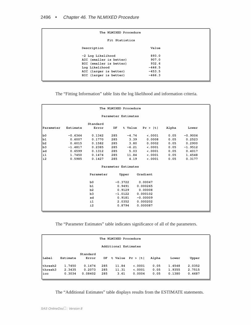
2496 � Chapter 46. The NLMIXED Procedure
The NLMIXED Procedure
Fit Statistics
Description Value
-2 Log Likelihood 893.0AIC (smaller is better) 907.0BIC (smaller is better) 932.6Log Likelihood -446.5AIC (larger is better) -453.5BIC (larger is better) -466.3
The “Fitting Information” table lists the log likelihood and information criteria.
The NLMIXED Procedure
Parameter Estimates
StandardParameter Estimate Error DF t Value Pr > |t| Alpha Lower
b0 -0.6364 0.1342 285 -4.74 <.0001 0.05 -0.9006b1 0.6007 0.1770 285 3.39 0.0008 0.05 0.2523b2 0.6015 0.1582 285 3.80 0.0002 0.05 0.2900b3 -1.4817 0.2385 285 -6.21 <.0001 0.05 -1.9512sd 0.6599 0.1312 285 5.03 <.0001 0.05 0.4017i1 1.7450 0.1474 285 11.84 <.0001 0.05 1.4548i2 0.5985 0.1427 285 4.19 <.0001 0.05 0.3177
Parameter Estimates
Parameter Upper Gradient
b0 -0.3722 0.00047b1 0.9491 0.000265b2 0.9129 0.00008b3 -1.0122 0.000102sd 0.9181 -0.00009i1 2.0352 0.000202i2 0.8794 0.000087
The “Parameter Estimates” table indicates significance of all of the parameters.
The NLMIXED Procedure
Additional Estimates
StandardLabel Estimate Error DF t Value Pr > |t| Alpha Lower Upper
thresh2 1.7450 0.1474 285 11.84 <.0001 0.05 1.4548 2.0352thresh3 2.3435 0.2073 285 11.31 <.0001 0.05 1.9355 2.7515icc 0.3034 0.08402 285 3.61 0.0004 0.05 0.1380 0.4687
The “Additional Estimates” table displays results from the ESTIMATE statements.
SAS OnlineDoc: Version 8

Example 46.4. Poisson-Normal Model with Count Data � 2497
Example 46.4. Poisson-Normal Model with Count Data
This example uses the pump failure data of Gaver and O’Muircheartaigh (1987). Thenumber of failures and the time of operation are recorded for 10 pumps. Each ofthe pumps is classified into one of two groups corresponding to either continuous orintermittent operation. The data are as follows.
data pump;input y t group;pump = _n_;logtstd = log(t) - 2.4564900;datalines;
5 94.320 11 15.720 25 62.880 1
14 125.760 13 5.240 2
19 31.440 11 1.048 21 1.048 24 2.096 2
22 10.480 2run;
Each row denotes data for a single pump, and the variable LOGTSTD contains thecentered operation times.
Letting yij denote the number of failures for thejth pump in theith group, Draper(1996) considers the following hierarchical model for these data:
yij j�ij � Poisson(�ij)
log �ij = �i + �i(log tij � log t) + eij
eij j�2 � Normal(0; �2)
The model specifies different intercepts and slopes for each group, and the randomeffect is a mechanism for accounting for overdispersion.
The corresponding PROC NLMIXED statements are as follows.
proc nlmixed data=pump;parms logsig 0 beta1 1 beta2 1 alpha1 1 alpha2 1;if (group = 1) then eta = alpha1 + beta1*logtstd + e;else eta = alpha2 + beta2*logtstd + e;lambda = exp(eta);model y ~ poisson(lambda);random e ~ normal(0,exp(2*logsig)) subject=pump;estimate ’alpha1-alpha2’ alpha1-alpha2;estimate ’beta1-beta2’ beta1-beta2;
run;
The output is as follows.
SAS OnlineDoc: Version 8

2498 � Chapter 46. The NLMIXED Procedure
The NLMIXED Procedure
Specifications
Description Value
Data Set WORK.PUMPDependent Variable yDistribution for Dependent Variable PoissonRandom Effects eDistribution for Random Effects NormalSubject Variable pumpOptimization Technique Dual Quasi-NewtonIntegration Method Adaptive Gaussian
Quadrature
The “Specifications” table displays some details for this Poisson-Normal model.
The NLMIXED Procedure
Dimensions
Description Value
Observations Used 10Observations Not Used 0Total Observations 10Subjects 10Max Obs Per Subject 1Parameters 5Quadrature Points 5
The “Dimensions” table indicates that data for 10 pumps are used with one observa-tion for each.
The NLMIXED Procedure
Parameters
logsig beta1 beta2 alpha1 alpha2 NegLogLike
0 1 1 1 1 32.8614614
The “Parameters” table lists the simple starting values for this problem and the initialevaluation of the negative log likelihood.
SAS OnlineDoc: Version 8

Example 46.4. Poisson-Normal Model with Count Data � 2499
The NLMIXED Procedure
Iteration History
Iter Calls NegLogLike Diff MaxGrad Slope
1 2 30.6986932 2.162768 5.107253 -91.6022 5 30.0255468 0.673146 2.761738 -11.04893 7 29.726325 0.299222 2.990401 -2.360484 9 28.7390263 0.987299 2.074431 -3.936785 10 28.3161933 0.422833 0.612531 -0.630846 12 28.09564 0.220553 0.462162 -0.526847 14 28.0438024 0.051838 0.405047 -0.100188 16 28.0357134 0.008089 0.135059 -0.018759 18 28.033925 0.001788 0.026279 -0.00514
10 20 28.0338744 0.000051 0.00402 -0.0001211 22 28.0338727 1.681E-6 0.002864 -5.09E-612 24 28.0338724 3.199E-7 0.000147 -6.87E-713 26 28.0338724 2.532E-9 0.000017 -5.75E-9
NOTE: GCONV convergence criterion satisfied.
The “Iterations” table indicates successful convergence in 13 iterations.
The NLMIXED Procedure
Fit Statistics
Description Value
-2 Log Likelihood 56.1AIC (smaller is better) 66.1BIC (smaller is better) 67.6Log Likelihood -28.0AIC (larger is better) -33.0BIC (larger is better) -33.8
The “Fitting Information” table lists the final log likelihood and associated informa-tion criteria.
SAS OnlineDoc: Version 8
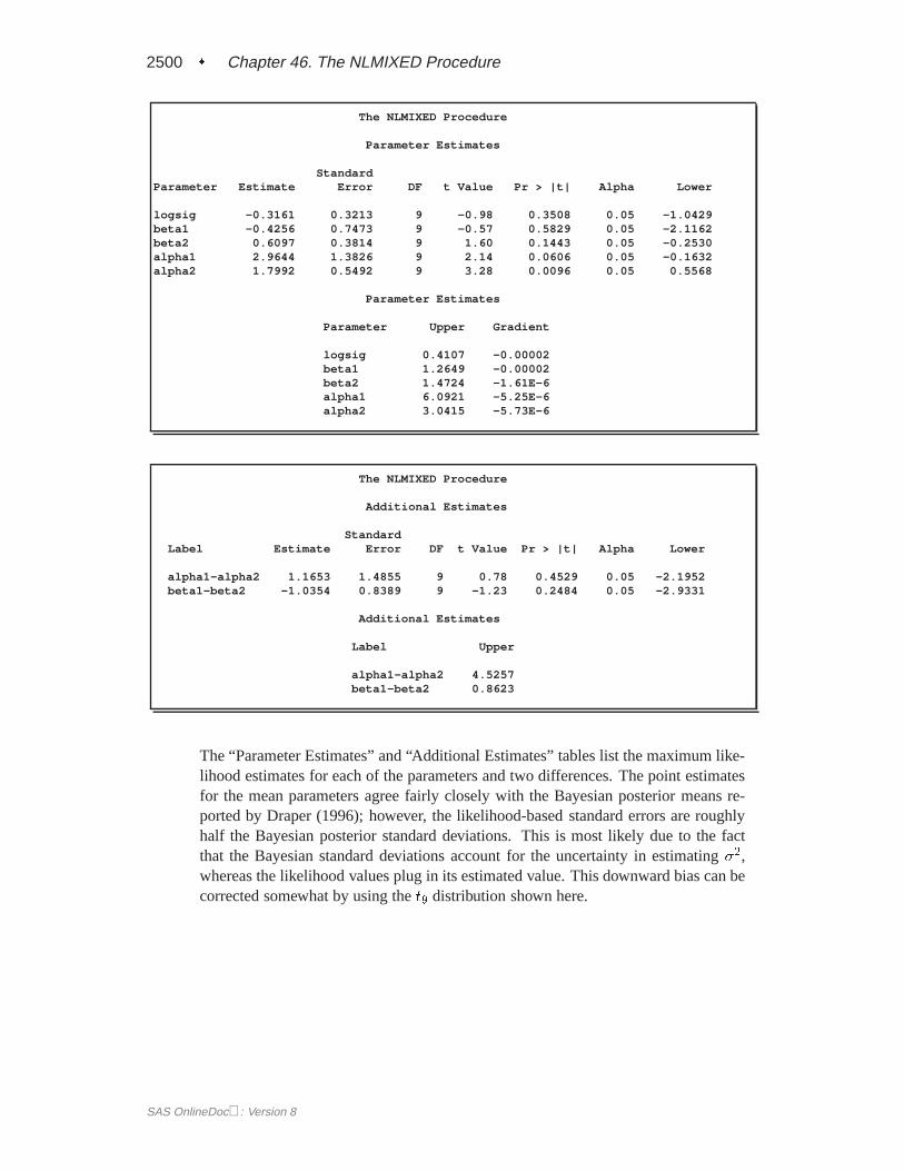
2500 � Chapter 46. The NLMIXED Procedure
The NLMIXED Procedure
Parameter Estimates
StandardParameter Estimate Error DF t Value Pr > |t| Alpha Lower
logsig -0.3161 0.3213 9 -0.98 0.3508 0.05 -1.0429beta1 -0.4256 0.7473 9 -0.57 0.5829 0.05 -2.1162beta2 0.6097 0.3814 9 1.60 0.1443 0.05 -0.2530alpha1 2.9644 1.3826 9 2.14 0.0606 0.05 -0.1632alpha2 1.7992 0.5492 9 3.28 0.0096 0.05 0.5568
Parameter Estimates
Parameter Upper Gradient
logsig 0.4107 -0.00002beta1 1.2649 -0.00002beta2 1.4724 -1.61E-6alpha1 6.0921 -5.25E-6alpha2 3.0415 -5.73E-6
The NLMIXED Procedure
Additional Estimates
StandardLabel Estimate Error DF t Value Pr > |t| Alpha Lower
alpha1-alpha2 1.1653 1.4855 9 0.78 0.4529 0.05 -2.1952beta1-beta2 -1.0354 0.8389 9 -1.23 0.2484 0.05 -2.9331
Additional Estimates
Label Upper
alpha1-alpha2 4.5257beta1-beta2 0.8623
The “Parameter Estimates” and “Additional Estimates” tables list the maximum like-lihood estimates for each of the parameters and two differences. The point estimatesfor the mean parameters agree fairly closely with the Bayesian posterior means re-ported by Draper (1996); however, the likelihood-based standard errors are roughlyhalf the Bayesian posterior standard deviations. This is most likely due to the factthat the Bayesian standard deviations account for the uncertainty in estimating�2,whereas the likelihood values plug in its estimated value. This downward bias can becorrected somewhat by using thet9 distribution shown here.
SAS OnlineDoc: Version 8

References � 2501
References
Abramowitz, M. and Stegun, I.A. (1972),Handbook of Mathematical Functions,New York: Dover Publications, Inc.
Anderson, D.A. and Aitkin, M. (1985), “Variance Component Models with BinaryResponse: Interviewer Variability,”Journal of the Royal Statistical Society B,47, 203–210.
Beal, S.L. and Sheiner, L.B. (1982), “Estimating Population Kinetics,”CRC Crit.Rev. Biomed. Eng.,8, 195–222.
Beal, S.L. and Sheiner, L.B. (1988), “Heteroskedastic Nonlinear Regression,”Tech-nometrics,30, 327–338.
Beal, S.L. and Sheiner, L.B., eds. (1992),NONMEM User’s Guide,University ofCalifornia, San Francisco, NONMEM Project Group.
Beale, E.M.L. (1972), “A Derivation of Conjugate Gradients,” inNumerical Methodsfor Nonlinear Optimization, ed. F.A. Lootsma, London: Academic Press.
Beitler, P.J. and Landis, J.R. (1985), “A Mixed-effects Model for Categorical Data,”Biometrics,41, 991–1000.
Billingsley, P. (1986),Probability and Measure,Second Edition, New York: JohnWiley & Sons, Inc.
Booth, J.G. and Hobert, J.P. (1998), “Standard Errors of Prediction in GeneralizedLinear Mixed Models,”Journal of the American Statistical Association,93,262–272.
Breslow, N.E. and Clayton, D.G. (1993), “Approximate Inference in Generalized Lin-ear Mixed Models,”Journal of the American Statistical Association,88, 9–25.
Cramer, J. S. (1986),Econometric Applications of Maximum Likelihood Methods,Cambridge, England: Cambridge University Press.
Crouch, E.A.C. and Spiegelman, D. (1990), “The Evaluation of Integrals of the FormR1�1
f(t) exp(�t2)dt: Application to Logistic-normal Models,”Journal of theAmerican Statistical Association,85, 464–469
Davidian, M. and Gallant, R.A. (1993), “The Nonlinear Mixed Effects Model with aSmooth Random Effects Density,”Biometrika,80, 475–488.
Davidian, M. and Giltinan, D.M. (1995),Nonlinear Models for Repeated Measure-ment Data,New York: Chapman & Hall.
Dennis, J.E., Gay, D.M., and Welsch, R.E. (1981), “An Adaptive Nonlinear Least-Squares Algorithm,”ACM Transactions on Mathematical Software, 7, 348–368.
Dennis, J.E. and Mei, H.H.W. (1979), “Two New Unconstrained Optimization Algo-rithms which Use Function and Gradient Values,”J. Optim. Theory Appl., 28,453–482.
Dennis, J.E. and Schnabel, R.B. (1983),Numerical Methods for Unconstrained Op-timization and Nonlinear Equations,Englewood, New Jersey: Prentice-Hall.
SAS OnlineDoc: Version 8
2502 � Chapter 46. The NLMIXED Procedure
Diggle, P.J., Liang, K.Y., and Zeger, S.L. (1994),Analysis of Longitudinal Data,Oxford: Clarendon Press.
Draper, D. (1996), “Discussion of the Paper by Lee and Nelder,”Journal of the RoyalStatistical Society, Series B, 58, 662–663.
Draper, N.R. and Smith, H. (1981),Applied Regression Analysis,Second Edition,New York: John Wiley & Sons, Inc.
Engel, B. and Keen, A. (1992), “A Simple Approach for the Analysis of General-ized Linear Mixed Models,” LWA-92-6, Agricultural Mathematics Group (GLW-DLO). Wageningen, The Netherlands.
Eskow, E. and Schnabel, R.B. (1991), “Algorithm 695: Software for a New Mod-ified Cholesky Factorization,”Transactions on Mathematical Software, 17(3),306–312.
Ezzet, F. and Whitehead, J. (1991), “A Random Effects Model for Ordinal Responsesfrom a Crossover Trial,”Statistics in Medicine,10, 901–907.
Fletcher, R. (1987),Practical Methods of Optimization,Second Edition, Chichester:John Wiley & Sons, Inc.
Galecki, A.T. (1998), “NLMEM: New SAS/IML Macro for Hierarchical NonlinearModels,”Computer Methods and Programs in Biomedicine,55, 107–216.
Gallant, A.R. (1987),Nonlinear Statistical Models, New York: John Wiley & Sons,Inc.
Gaver, D.P. and O’Muircheartaigh, I.G. (1987), “Robust Empirical Bayes Analysisof Event Rates,”Technometrics, 29, 1–15.
Gay, D.M. (1983), “Subroutines for Unconstrained Minimization,”ACM Transac-tions on Mathematical Software, 9, 503–524.
Gilmour, A.R., Anderson, R.D., and Rae, A.L. (1985), “The Analysis of BinomialData by Generalized Linear Mixed Model,”Biometrika,72, 593–599.
Goldstein, H. (1991), “Nonlinear Multilevel Models, with an Application to DiscreteResponse Data,”Biometrika,78, 45–51.
Golub, G.H., and Welsch, J.H. (1969), “Calculation of Gaussian Quadrature Rules,”Mathematical Computing,23, 221–230.
Harville, D.A. and Mee, R.W. (1984), “A Mixed-model Procedure for AnalyzingOrdered Categorical Data,”Biometrics,40, 393–408.
Hedeker, D. and Gibbons, R.D. (1994), “A Random Effects Ordinal RegressionModel for Multilevel Analysis,”Biometrics,50, 933–944.
Lin, X. and Breslow, N.E. (1996), “Bias Correction in Generalized Linear MixedModels with Multiple Components of Dispersion,”Journal of the American Sta-tistical Association,91, 1007–1016.
Lindstrom, M.J. and Bates, D.M. (1990), “Nonlinear Mixed Effects Models for Re-peated Measures Data,”Biometrics,46, 673–687.
SAS OnlineDoc: Version 8
References � 2503
Littell, R.C., Milliken, G.A., Stroup, W.W., and Wolfinger, R.D. (1996),SAS Systemfor Mixed Models,Cary, NC: SAS Institute Inc.
Liu, Q. and Pierce, D.A. (1994), “A Note on Gauss-Hermite Quadrature,”Biometrika,81, 624–629.
Longford, N.T. (1994), “Logistic Regression with Random Coefficients,”Computa-tional Statistics and Data Analysis,17, 1–15.
McCulloch, C.E. (1994), “Maximum Likelihood Variance Components Estimationfor Binary Data,”Journal of the American Statistical Association,89, 330–335.
McGilchrist, C.E. (1994), “Estimation in Generalized Mixed Models,”Journal of theRoyal Statistical Society B,56, 61–69.
Moré, J.J. (1978), “The Levenberg-Marquardt Algorithm: Implementation and The-ory,” in Lecture Notes in Mathematics 630, ed. G.A. Watson, Berlin-Heidelberg-New York: Springer Verlag.
Moré, J.J. and Sorensen, D.C. (1983), “Computing a Trust-region Step,”SIAM Jour-nal on Scientific and Statistical Computing, 4, 553–572.
Ochi, Y. and Prentice, R.L. (1984), “Likelihood Inference in a Correlated Probit Re-gression Model,”Biometrika,71, 531–543.
Pierce, D.A. and Sands, B.R. (1975),Extra-Bernoulli Variation in Binary Data,Tech-nical Report 46, Department of Statistics, Oregon State University.
Pinheiro, J.C. and Bates, D.M. (1995), “Approximations to the Log-likelihood Func-tion in the Nonlinear Mixed-effects Model,”Journal of Computational andGraphical Statistics,4, 12–35.
Polak, E. (1971),Computational Methods in Optimization, New York, AcademicPress.
Powell, J.M.D. (1977), “Restart Procedures for the Conjugate Gradient Method,”Math. Prog., 12, 241–254.
Roe, D.J. (1997) “Comparison of Population Pharmacokinetic Modeling MethodsUsing Simulated Data: Results from the Population Modeling Workgroup,”Statistics in Medicine,16, 1241–1262.
Rodriguez, G. and Goldman, N. (1995), “An Assessment of Estimation Proceduresfor Multilevel Models with Binary Response,”Journal of the Royal StatisticalSociety, Series A,158, 73–89.
Schall, R. (1991). “Estimation in Generalized Linear Models with Random Effects,”Biometrika, 78, 719–727.
Schittkowski, K. and Stoer, J. (1979), “A Factorization Method for the Solu-tion of Constrained Linear Least Squares Problems Allowing Subsequent DataChanges,”Numererische Mathematik, 31, 431–463.
Serfling, R.J. (1980),Approximation Theorems of Mathematical Statistics,New York,John Wiley & Sons, Inc.
SAS OnlineDoc: Version 8
2504 � Chapter 46. The NLMIXED Procedure
Sheiner L. B. and Beal S. L., “Evaluation of Methods for Estimating Population Phar-macokinetic Parameters. I. Michaelis-Menten Model: Routine Clinical Pharma-cokinetic Data,”Journal of Pharmacokinetics and Biopharmaceutics,8, (1980)553–571.
Sheiner, L.B. and Beal, S.L. (1985), “Pharmacokinetic Parameter Estimates fromSeveral Least Squares Procedures: Superiority of Extended Least Squares,”Jour-nal of Pharmacokinetics and Biopharmaceutics,13, 185–201.
Stiratelli, R., Laird, N.M., and Ware, J.H. (1984), “Random Effects Models for SerialObservations with Binary Response,”Biometrics,40, 961-971.
Vonesh, E.F., (1992), “Nonlinear Models for the Analysis of Longitudinal Data,”Statistics in Medicine,11, 1929–1954.
Vonesh, E.F., (1996), “A Note on Laplace’s Approximation in Nonlinear Mixed Ef-fects Models,”Biometrika,83, 447–452.
Vonesh, E.F. and Chinchilli, V.M. (1997),Linear and Nonlinear Models for the Anal-ysis of Repeated Measurements,New York: Marcel Dekker.
Weil, C.S. (1970), “Selection of the Valid Number of Sampling Units and Consid-eration of their Combination in Toxicological Studies Involving Reproduction,Teratogenesis, or Carcinogenesis,”Food and Cosmetic Toxicology,8, 177–182.
Williams, D.A. (1975), “The Analysis of Binary Responses from Toxicological Ex-periments Involving Reproduction and Teratogenicity,”Biometrics,31, 949–952.
Wolfinger R.D. (1993), “Laplace’s Approximation for Nonlinear Mixed Models,”Biometrika,80, 791–795.
Wolfinger, R.D. (1997), “Comment: Experiences with the SAS Macro NLINMIX,”Statistics in Medicine,16, 1258–1259.
Wolfinger, R.D., and Lin, X. (1997), “Two Taylor-series Approximation Methodsfor Nonlinear Mixed Models,”Computational Statistics and Data Analysis,25,465–490.
Wolfinger, R.D. and O’Connell, M. (1993), “Generalized Linear Mixed Models: aPseudo-likelihood Approach,”Journal of Statistical Computation and Simula-tion, 48, 233–243.
Yuh, L., Beal, S., Davidian, M., Harrison, F., Hester, A., Kowalski, K., Vonesh, E.,Wolfinger, R. (1994), “Population Pharmacokinetic/Pharmacodynamic Method-ology and Applications: a Bibliography,”Biometrics,50, 566–575.
SAS OnlineDoc: Version 8

The correct bibliographic citation for this manual is as follows: SAS Institute Inc.,SAS/STAT ® User’s Guide, Version 8, Cary, NC: SAS Institute Inc., 1999.
SAS/STAT® User’s Guide, Version 8Copyright © 1999 by SAS Institute Inc., Cary, NC, USA.ISBN 1–58025–494–2All rights reserved. Produced in the United States of America. No part of this publicationmay be reproduced, stored in a retrieval system, or transmitted, in any form or by anymeans, electronic, mechanical, photocopying, or otherwise, without the prior writtenpermission of the publisher, SAS Institute Inc.U.S. Government Restricted Rights Notice. Use, duplication, or disclosure of thesoftware and related documentation by the U.S. government is subject to the Agreementwith SAS Institute and the restrictions set forth in FAR 52.227–19 Commercial ComputerSoftware-Restricted Rights (June 1987).SAS Institute Inc., SAS Campus Drive, Cary, North Carolina 27513.1st printing, October 1999SAS® and all other SAS Institute Inc. product or service names are registered trademarksor trademarks of SAS Institute Inc. in the USA and other countries.® indicates USAregistration.Other brand and product names are registered trademarks or trademarks of theirrespective companies.The Institute is a private company devoted to the support and further development of itssoftware and related services.


![ORSON PARLEY BATES SR LIFE SKETCH - Ames Family...ORSON PARLEY BATES SR LIFE SKETCH 3 March 1836 – 5 January 1899 BY HIS SON, ORMUS ARIAH BATES [1836] Orson Parley Bates Sr, the](https://static.fdocuments.in/doc/165x107/6036ee78251f5076a613ccc8/orson-parley-bates-sr-life-sketch-ames-family-orson-parley-bates-sr-life-sketch.jpg)