Discussion Papers No. 652, May 2011 Statistics Norway, Research Department

Pål Boug, Ådne Cappelen and Anders R. Swensen

The new Keynesian Phillips curve: Does it fit Norwegian data?

Abstract:

We evaluate the empirical performance of the new Keynesian Phillips curve (NKPC) for a small open economy using cointegrated vector autoregressive models, likelihood based methods and general method of moments. Our results indicate that both baseline and hybrid versions of the NKPC as well as exact and inexact formulations of the rational expectation hypothesis are most likely at odds with Norwegian data. By way of contrast, we establish a well-specified dynamic backward-looking imperfect competition model (ICM), a model which encompasses the NKPC in-sample with a major monetary policy regime shift from exchange rate targeting to inflation targeting. We also demonstrate that the ICM model forecasts well both post-sample and during the recent financial crisis. Our findings suggest that taking account of forward-looking behaviour when modelling consumer price inflation is unnecessary to arrive at a well-specified model by econometric criteria.

Keywords: The new Keynesian Phillips curve, imperfect competition model, cointegrated vector autoregressive models (CVAR), equilibrium correction models, likelihood based methods and general method of moments (GMM).

JEL classification: C51, C52, E31, F31

Acknowledgements: The authors thank Ida Wolden Bache, Neil R. Ericsson, David F. Hendry, Eilev Jansen, Katarina Juselius, Ragnar Nymoen, Terje Skjerpen and J-P Urbain for valuable comments and discussions. The procedure "optim" in the statistical package R [see http://www.r-project.org/ and R Development Core team (2006)] was used to carry out tests of the exact NKPC model within vector autoregressive models and likelihood based methods. The GMM results of the inexact NKPC were produced by EViews6 [see EViews6 (2007)], while the modelling of the backward-looking ICM model was performed by OxMetrics 6 [see Doornik and Hendry (2009)]. Data underlying the empirical analysis and test results referred to in the paper are available from the authors upon request.

Address: Pål Boug, Statistics Norway, Research Department. E-mail: bou@ssb.no

Ådne Cappelen, Statistics Norway, Research Department. E-mail: cap@ssb.no

Anders R. Swensen, University of Oslo, Department of Mathematics. E-mail: swensen@math.uio.no

Discussion Papers comprise research papers intended for international journals or books. A preprint of a Discussion Paper may be longer and more elaborate than a standard journal article, as it may include intermediate calculations and background material etc.

© Statistics Norway Abstracts with downloadable Discussion Papers in PDF are available on the Internet: http://www.ssb.no http://ideas.repec.org/s/ssb/dispap.html For printed Discussion Papers contact: Statistics Norway Telephone: +47 62 88 55 00 E-mail: Salg-abonnement@ssb.no ISSN 0809-733X Print: Statistics Norway

3

Sammendrag

Vi undersøker hvor godt den nykeynesianske Phillipskurven for en liten åpen økonomi passer til

norske forhold. Modellen tilsier at løpende konsumprisvekst avhenger av forventet konsumprisvekst i

neste periode og avvik mellom nivået på konsumprisene og prisene på arbeidskraft og import av varer

og tjenester. Våre funn indikerer at modellen ikke får støtte med norske data når vi legger standard

statistiske kriterier til grunn. Vi finner isteden støtte for en konkurrerende modell som inneholder

betydelige effekter av konsumprisveksten i tidligere perioder i tillegg til effekter fra avviket mellom

nivået på konsumprisene og prisene på arbeidskraft og import av varer og tjenester. Den

konkurrerende modellen forklarer konsumprisveksten rimelig godt i estimeringsperioden, en periode

som inkluderer overgangen fra valutakursstyring til inflasjonsstyring i pengepolitikken. Samtidig er

den konkurrerende modellen i stand til å prognostisere konsumprisveksten nokså godt etter

estimeringsperioden og gjennom finanskrisen som var en ganske turbulent periode for norsk økonomi.

Våre funn indikerer at framoverskuende forventninger i prissettingen ikke synes å være viktig som

forklaringsvariabel ved modellering av den norske konsumprisveksten.

1 IntroductionWithin the new Keynesian economics paradigm, based on rational expectations, op-timising agents and imperfect competition in markets for goods, the new KeynesianPhillips curve (henceforth NKPC) is the workhorse of understanding in�ation dy-namics. The baseline NKPC explains current in�ation by expected future in�ationand real marginal costs as the forcing variable, whereas the hybrid version of themodel also includes lagged in�ation terms as a way of modelling "rule of thumb"or backward-looking price setters. Since the in�uential papers by Galí and Gertler(1999) and Galí et al. (2001), who claim strong evidence in favour of the NKPCusing European and US post-war data, a great number of studies have tested theempirical validity of the model based on data of both closed and open economies,see e.g. Boug et al. (2010), Tillmann (2009), Juillard et al. (2008), Bjørnstad andNymoen (2008), Gogley and Sbordone (2008), Fanelli (2008), Kurmann (2007), Ba-tini et al. (2005), Bårdsen et al. (2004, 2005) and Kara and Nelson (2003) amongothers. The studies di¤er with respect to data used, sample period studied andeconometric methods applied, and the supportive evidence on the NKPC is rathermixed.

The open economy new Keynesian Phillips curve (henceforth OE-NKPC) dif-fers from its closed economy counterpart in that the exchange rate and prices onimported goods matter in some way or another for domestic in�ation. In the empir-ical OE-NKPC literature two approaches have basically been undertaken to modelthe hypothesised connection between the exchange rate and domestic in�ation. The�rst approach involves treating imported goods as �nal consumer goods and henceintroducing import prices directly into the de�nition of consumer prices. In sodoing, the real exchange rate becomes an explanatory variable in addition to ex-pected future in�ation and real marginal costs in the NKPC model, see Bjørnstadand Nymoen (2008), Guender and Xie (2007), Guender (2006), Galí and Monacelli(2005) and Giordani (2004) for examples. The second approach involves introducingimported goods as intermediate inputs which, together with labour, produce �nalconsumer goods. Accordingly, real marginal costs in production becomes a functionof relative prices of imported inputs, see e.g. Batini et al. (2005), Kara and Nelson(2003) and McCallum and Nelson (1999).1

The two approaches have mainly been investigated from a theoretical perspec-tive in the literature. Among the relatively few existing empirical studies, Bjørnstadand Nymoen (2008) introduce open economy features by means of the �rst approachand conclude that the OE-NKPC is most likely at odds with a panel data set oftwenty OECD countries (including Norway). Guender and Xie (2007) also argue, us-

1Smets and Wouters (2002) combine the two approaches in their theoretical NKPC model byintroducing imported goods as both intermediate inputs as well as �nal consumer goods. Svensson(2000) discusses the channels through which the exchange rate is likely to a¤ect consumer pricesin the NKPC model for small open economies.

4

ing the �rst approach, that the OE-NKPC does not receive much empirical supportbased on a data set of six open economies. Kara and Nelson (2003), on the otherhand, apply the second approach and claim that the OE-NKPC matches reasonablywell with UK data. Batini et al. (2005) also derive versions of the OE-NKPC withaccommodating results on UK data. Although imports are theoretically modelledas intermediate inputs in that study, the empirical models are more in line withimports being modelled as �nal goods as prices of total imports (and not prices ofimported material inputs) are used among the explanatory variables. Nevertheless,the rather mixed results with respect to the empirical status of the OE-NKPC callfor further research.

In this paper, we evaluate by means of the �rst approach the empirical per-formance of the OE-NKPC for Norway, a small open economy where internationaltrade plays an important role in the exchange of goods and services. Hence, theexchange rate through import prices is likely to be relevant in the determination ofdomestic in�ation. We derive an OE-NKPC for Norwegian in�ation based on theforward-looking linear quadratic adjustment cost model of Rotemberg (1982) andthe theoretical principles of the imperfect competition model (henceforth ICM) fora small open economy. Our OE-NKPC thereby relates current in�ation to expectedfuture in�ation and the di¤erence between the actual price and the price target inlevels as a theory consistent forcing variable, the latter hypothesised to be based ona weigthed average of unit labour costs and prices of total imports. We contribute tothe existing OE-NKPC literature by focusing on both baseline and hybrid models aswell as on exact formulations in the sense of Hansen and Sargent (1991) and inexactformulations in which a stochastic term is included in the models. To this end, weemploy the likelihood based testing procedures suggested by Johansen and Swensen(1999, 2004, 2008) and the commonly used GMM procedure when evaluating theexact and the inexact versions of our OE-NKPC, respectively. Rather than usingan arbitrary instrument set, which is often the case in related studies, we let theinstruments used within the GMM framework be dictated from �tted VAR modelsunderlying the testing of the exact OE-NKPC. We are consequently able to shedsome light on the importance of introducing a stochastic error term to the empiricalmodels, an often neglected econometric issue in the literature. Unlike many relatedstudies, we pay particular attention to time series properties, and possibly cointe-grated nature, of variables involved by means of �tted VAR models and likelihoodbased inference.

Our empirical investigation produces several noteworthy �ndings. First, weestablish a well-speci�ed empirical counterpart to the theory-consistent forcing vari-able. Accordingly, the hypothesised link between domestic in�ation and the ex-change rate through import prices in our OE-NKPC is supported using Norwegiandata. These �ndings are also in line with existing models of in�ation based on Nor-wegian data. Second, and by way of contrast, we demonstrate that both baselineand hybrid versions as well as exact and inexact formulations of our OE-NKPC are

5

most likely at odds with the data. Hence, the forward-looking part of our OE-NKPCis rejected, whereas the part of the model containing the deviation of the price levelfrom its target is not. Finally, we establish a well-speci�ed dynamic ICM modelof in�ation with backward-looking elements only, a model which encompasses theOE-NKPC in-sample with a major monetary policy regime shift from exchange ratetargeting to in�ation targeting. The regime robustness of the dynamic ICM modelis inconsistent with the Lucas-critique being quantitatively important in our case.Also, we �nd that the dynamic ICM model forecasts well post-sample and duringthe �nancial crisis in 2008 and 2009 when the exchange rate �uctuated considerably.

The rest of the paper is organised as follows: Section 2 outlines our OE-NKPC,Section 3 describes the data, Section 4 reports �ndings from the cointegration analy-sis, Section 5 reports the various tests of the OE-NKPC and Section 6 develops adynamic backward-looking ICM model as a competing model of in�ation and con-ducts a forecasting exercise on that model. Section 7 concludes.

2 An open economy NKPC modelAs explained by Roberts (1995), there are several routes from a theoretical set up of�rm�s pricing behaviour that lead to the NKPCmodel, including the forward-lookinglinear quadratic adjustment cost model of Rotemberg (1982) and the models ofstaggered contracts developed by Taylor (1979, 1980) and Calvo (1983). We assumethat the representative �rm, based on Rotemberg (1982), chooses a sequence ofprices (Pt+j) to minimise the loss function

(1) Et

" 1Xj=1

�j��(pt+j � p�t+j)2 + (pt+j � pt+j�1)2

�#;

where Et denotes the conditional expectation given the information contained inthe information set at time t and lower case letters indicate natural logarithms ofa variable, i.e., pt+j =ln(Pt+j).2 The variable p�t is the price target or the staticequilibrium price, whereas � represents the discount rate and � the relative costparameter of the two terms of the loss function. Hence, �rms determine a sequence ofprices so as to minimise the expected present discounted value of the sum of all futuresquared deviations from the target and squared changes in the price itself. Becausechanges in the price will be penalised, immediate adjustment towards the targetwill be non-optimal unless � is large. The �rst order condition of this minimisationproblem gives the Euler equation

(2) �pt = �Et�pt+1 � �(pt � p�t );2Throughout the paper, lower case letters denote natural logarithms of the corresponding upper

case variables.

6

where the �rst di¤erence of pt, �pt = pt � pt�1, de�nes current in�ation, whileEt�pt+1 is expected in�ation one period ahead conditional upon information avail-able at time t.

We now show how to introduce, from theoretical principles, open economyfeatures into (2). Building on existing ICM models of in�ation for Norway, see e.g.Bårdsen et al. (2005, ch. 8.7), we assume that the representative �rm operates inimperfectly competitive markets facing regular downward sloping demand curves.Pro�t maximisation then implies that prices are set as a mark-up over marginalcosts. Assuming a value added Cobb-Douglas production function in labour andcapital with capital as a quasi-�xed factor, unit labour costs are proportional tomarginal costs. We follow Bjørnstad and Nymoen (2008) and Batini et al. (2005)among others and let the mark-up depend on relative prices such that

(3) pdt = m0 �m1(pdt � pit) + ulct;

where pdt denotes the price level on domestic consumer goods and services, pit isthe price level on imported consumer goods and services, ulct denotes unit labourcosts and 0 � m1 � 1 and re�ects conditions on the demand side of the productmarkets. It follows from (3) that an increase in the competing price allows thedomestic producer to increase her mark-up over unit labour costs. We then let(1 � �) denote the constant import share and de�ne the aggregate consumer pricelevel by the commonly used identity of the form [see e.g. Svensson (2000), Galí andMonacelli (2005) and Bjørnstad and Nymoen (2008)]

(4) pt � �pdt + (1� �)pit:

By using (4), we can solve for the producer�s price target to obtain

(5) pt = 0 + 1ulct + 2pit;

where 0 = m0 1, 1 = �=(1 + m1) and 2 = (1 � 1). We notice that (5) ishomogeneous of degree one in competing prices and unit labour costs. Although(5) is derived from the ICM model, it also contains the law of one price or perfectcompetition for homogenous goods as a special case. In the latter casem1 approachesin�nity, such that the domestic price is equal to the cometing price, i.e., pdt = pit.Intuitively, this is reasonable because the closer substitutes the products are thesmaller is the market power of each producer and accordingly also the mark-up.Our speci�cation of the mark-up allows for a general model to be tested, with aconstant mark-up as a special case.3 Equation (5) is a static model of the price

3In the closed economy NKPC literature it is common to assume that producers face isoelasticdemand curves so that the mark-up is a constant, see e.g. Galí and Gertler (1999) and Galí et al.(2001).

7

target so that the right hand side of (5) is equivalent to p�t in (2). Inserting (5) in(2) yields the baseline OE-NKPC model in our context

(6) �pt = �Et�pt+1 � �eqcmt;

where eqcmt = pt � 0 � 1ulct � 2pit. Before looking at the hybrid version of (6),we point out that the dynamic backward-looking ICM model, without any forward-lokking term, is a special case of the OE-NKPC. To see this, we may reparameterise(6) such that

(7) �pt = �1Et�pt+1 + �2�ulct + �3�pit � �4eqcmt�1;

where �1 = �=(1 + �), �2 = � 1=(1 + �), �3 = � 2=(1 + �) and �4 = �=(1 + �). Thedynamic backward-looking ICM model is therefore nested by and is a special caseof the OE-NKPC when �1 = 0. If the hypothesis �1 = 0 cannot be rejected the OE-NKPC is said to be parsimoniously encompassed by the dynamic backward-lookingICM model in the terminology of Hendry (1995).4 Such a test outcome is furtherinconsistent with the main assumption of the NKPC that a signi�cant proportionof price setters are forward looking in accordance with the rational expectationhypothesis.

Inspired by the in�uencial studies by Galí and Gertler (1999) and Galí, Gertlerand López-Salido (2001), we specify the following hybrid version of (6) with bothforward-looking and backward-looking elements included:

(8) �pt = fEt�pt+1 + b�pt�1 � �heqcmt:

We see that (8) reduces to (6) when b = 0. Accordingly, if the baseline OE-NKPCis valid, then f = �, b = 0 and �h = �. Generally, the parameter spaces 0 � � � 1,0 � � and 0 � f ; b � 1, 0 � �h are required to provide an admissible economicinterpretation of an estimated baseline and hybrid OE-NKPC, respectively. If weregard in�ation as a stationary process, the deviation of the price level from itstarget value must also be a stationary process in order for (6) and (8) to be balancedequations. We notice that the expression eqcmt in (6) and (8) is a theory-consistentdriving variable that may form a cointegration relationship with testable restrictions.

The open economy NKPC in Batini et al. (2005) is consistent with and has thesame form and interpretation as (6), see Appendix 1 for details. However, as opposedto Batini et al. (2005), we pay particular attention to the time series properties, andpossibly cointegrated nature, of variables involved. We test the empirical relevanceof (6), (7) and (8) based on Norwegian data, cointegration techniques, likelihoodbased methods and GMM.

4Generally speaking, parsimonious encompassing requires a small model to explain the resultsof a larger model within which it is nested, cf. Hendry (1995, p. 511).

8

3 DataThe empirical analysis is based on quarterly, seasonally unadjusted data that spansthe period 1982Q1� 2009Q4, of which data from the period 1982Q1� 2005Q4 and2006Q1 � 2009Q4 are used for estimation and out-of -sample forecasting, respec-tively. Mavroeidis (2004) concludes that the estimates of the NKPC are less reliablewhen the sample covers periods in which in�ation has been under e¤ective policycontrol. The starting point of our estimation period is thus motivated by the factthat the 1970s and the early 1980s were characterised by massive governmental pricecontrols. If the expectational term in the OE-NKPC relationship is the most impor-tant in�uences on the correlation between exchange rate movements and in�ation,then we would expect the relationship to depend closely on monetary policy regimein force. We explored this hypothesis by ending the estimation period in 2001Q1rather than in 2005Q4 as monetary policy changed fundamentally from exchangerate targeting to in�ation targeting in late March 2001.5 It turned out, however,that the estimates of both the OE-NKPC and the dynamic backward-looking ICMmodel are virtually unchanged irrespective of which of the two ending points is used.These �ndings suggest that the Lucas critique lacks force in our empirical case. Weextend the estimation sample by sixteen quarters for out-of -sample forecasting toshed light on any change in the link between exchange rates movements and domesticin�ation following the �nancial crisis in 2008 and 2009.

In line with Bårdsen et al. (2005), we measure quarterly in�ation by the o¢ cialconsumer price index rather than by the GDP de�ator normally used in the NKPCliterature. The actual prices that agents in the economy set are on gross outputand not on value added. De�ators based on value added are typically residuals inthe national accounts, in particular those following the principle of double-de�ating.Hence, the GDP de�ator is less related to the micro price setting behaviour thanother concept within the national account. Thus, we argue that the consumer priceindex is a more relevant price series for evaluating the OE-NKPC for Norway thanthe GDP de�ator. We employ the de�ator for total imports as a proxy for the pricelevel on imported consumer goods and services, whereas total labour costs relativeto value added in the private mainland economy serves as a proxy for unit labourcosts, see Appendix 2 for details. Figure 1 displays the log of the consumer priceindex (pt), the log of the import prices (pit) and the log of unit labour costs (ulct),together with the in�ation rates (�pt) over the sample period.

We notice that the consumer price in�ation shows rather large changes inthe quarters 1986Q3, 2001Q3, 2003Q1 and 2003Q2 during the estimation period.These changes are most likely associated with the 12 per cent devaluation of theNorwegian currency in May 1986, the drop in the VAT rate on food from 24 percent to 12 per cent in July 2001 and the substantial increase and decrease of theelectricity prices during the �rst and second quarter of 2003, respectively. That

5See Boug et al. (2006) for details.

9

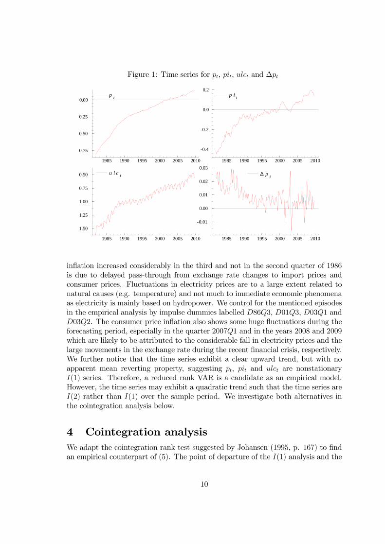
Figure 1: Time series for pt, pit, ulct and �pt

p t

1985 1990 1995 2000 2005 2010

­0.75

­0.50

­0.25

0.00p t p i t

1985 1990 1995 2000 2005 2010

­0.4

­0.2

0.0

0.2p i t

u l c t

1985 1990 1995 2000 2005 2010

­1.50

­1.25

­1.00

­0.75

­0.50 u l c t ∆ p t

1985 1990 1995 2000 2005 2010

­0.01

0.00

0.01

0.02

0.03∆ p t

in�ation increased considerably in the third and not in the second quarter of 1986is due to delayed pass-through from exchange rate changes to import prices andconsumer prices. Fluctuations in electricity prices are to a large extent related tonatural causes (e.g. temperature) and not much to immediate economic phenomenaas electricity is mainly based on hydropower. We control for the mentioned episodesin the empirical analysis by impulse dummies labelled D86Q3, D01Q3, D03Q1 andD03Q2. The consumer price in�ation also shows some huge �uctuations during theforecasting period, especially in the quarter 2007Q1 and in the years 2008 and 2009which are likely to be attributed to the considerable fall in electricity prices and thelarge movements in the exchange rate during the recent �nancial crisis, respectively.We further notice that the time series exhibit a clear upward trend, but with noapparent mean reverting property, suggesting pt, pit and ulct are nonstationaryI(1) series. Therefore, a reduced rank VAR is a candidate as an empirical model.However, the time series may exhibit a quadratic trend such that the time series areI(2) rather than I(1) over the sample period. We investigate both alternatives inthe cointegration analysis below.

4 Cointegration analysisWe adapt the cointegration rank test suggested by Johansen (1995, p. 167) to �ndan empirical counterpart of (5). The point of departure of the I(1) analysis and the

10

tests that follow is an equilibrium correction representation of a p-dimensional VARof order k written as

(9) �Xt =

k�1Xi=1

�i�Xt�i +�Xt�1 + �0Dt + �1 + �2t+ "t; t = k + 1; : : : ; T;

where Xt = (pt; ulct; pit)0, Dt includes seasonal dummies labelled SDit (i = 1; 2; 3)

and the impulse dummies D86Q3, D01Q3, D03Q1 and D03Q2 as described above,t is a linear deterministic trend and "k+1; : : : ; "T are independent Gaussian variableswith expectation zero and (unrestricted) covariance matrix . The initial obser-vations of X1; : : : ; Xk are kept �xed. We follow common practice and restrict thelinear trend to lie in the cointegrating space, whereas the deterministic componentsDt and �1 are kept unrestricted in (9). IfXt is I(1), presence of cointegration implies0 < r < p, where r denotes the rank or the number of cointegrating vectors of theimpact matrix �. The null hypothesis of r cointegrating vectors may be formulatedas H0: � = ��

0, where � and � are p x r matrices, �0Xt comprises r cointegratingI(0) linear combinations and � contains the adjustment coe¢ cients.

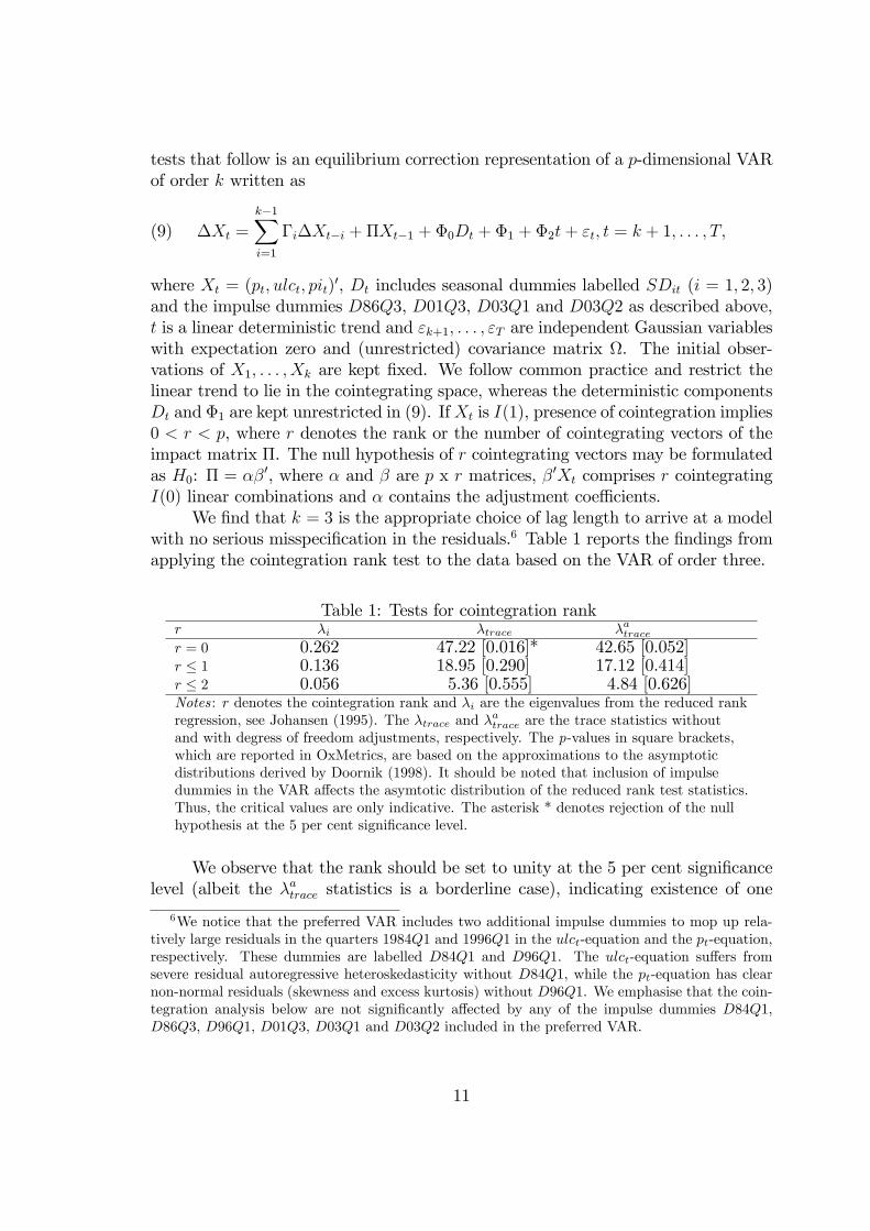
We �nd that k = 3 is the appropriate choice of lag length to arrive at a modelwith no serious misspeci�cation in the residuals.6 Table 1 reports the �ndings fromapplying the cointegration rank test to the data based on the VAR of order three.

Table 1: Tests for cointegration rankr �i �trace �atracer = 0 0.262 47.22 [0.016]* 42.65 [0.052]r � 1 0.136 18.95 [0.290] 17.12 [0.414]r � 2 0.056 5.36 [0.555] 4.84 [0.626]Notes: r denotes the cointegration rank and �i are the eigenvalues from the reduced rankregression, see Johansen (1995). The �trace and �

atrace are the trace statistics without

and with degress of freedom adjustments, respectively. The p-values in square brackets,which are reported in OxMetrics, are based on the approximations to the asymptoticdistributions derived by Doornik (1998). It should be noted that inclusion of impulsedummies in the VAR a¤ects the asymtotic distribution of the reduced rank test statistics.Thus, the critical values are only indicative. The asterisk * denotes rejection of the nullhypothesis at the 5 per cent signi�cance level.

We observe that the rank should be set to unity at the 5 per cent signi�cancelevel (albeit the �atrace statistics is a borderline case), indicating existence of one

6We notice that the preferred VAR includes two additional impulse dummies to mop up rela-tively large residuals in the quarters 1984Q1 and 1996Q1 in the ulct-equation and the pt-equation,respectively. These dummies are labelled D84Q1 and D96Q1. The ulct-equation su¤ers fromsevere residual autoregressive heteroskedasticity without D84Q1, while the pt-equation has clearnon-normal residuals (skewness and excess kurtosis) without D96Q1. We emphasise that the coin-tegration analysis below are not signi�cantly a¤ected by any of the impulse dummies D84Q1,D86Q3, D96Q1, D01Q3, D03Q1 and D03Q2 included in the preferred VAR.

11

cointegration relationship between consumer prices, unit labour costs and importprices. Testing the I(2) hypothesis by means of Johansen (1995), which combinestesting the rank of � as before and the potential additional reduced rank restrictionon the long run matrix of the model in �rst di¤erences, proposes that the numberof I(2) relations is zero in our case. It may be that including a quadratic deter-ministic trend would yield an even more satisfactory model �t. From an economicperspective, however, such a trend in levels of the variables is not a sensible longrun property.

The null hypothesis that the linear trend can be eliminated from the VAR, as-suming the rank to be unity, is not rejected by a likelihood ratio test. The p-value is0.388 based on a �2 approximation with one degree of freedom. The correspondingmaximised value of the 2 log likelihood, to be used in Section 5.1, is 2536:72. Impos-ing a further restriction of homogeneity between pt, ulct and pit entails a reductionin the value of the 2 log likelihood of 0:00097, which corresponds to a p-value of0:912 using the same �2 approximation. The issue of joint weak exogeneity of ulctand pit is more debatable. Here the �2 log likelihood ratio value is 7:909. The p-value based on approximating the null distribution with a �2 distribution with twodegrees of freedom is 0:02. However, investigating weak exogeneity more closely,using both parametric and non-parametric bootstrap methods, reveals that the as-ymptotic approximations are not accurate in our case. A bootstrap of the likelihoodratio test, using the estimated values of the VAR coe¢ cients not imposing weakexogeneity and resampling the residuals, yields a p-value of 0:515. The outcome ofa non-parametric bootstrap is similar. Hence, we conclude that the cointegrationvector enters the �pt-equation only.

We obtain the following restricted cointegrating vector (normalised on pt) whenthe restrictions of homogeneity between pt, ulct and pit, weak exogeneity of bothulct and pit and no linear trend in � are imposed (standard errors in parenthesis):

(10) pt = const:+ 0:604(0:084)

ulct + 0:396pit:

To sum up, we interpret (10) as a long-run consumer price equation that cor-responds well with the theory of mark-up prising and that for a small open economylike the Norwegian, open economy features such as import prices are expected tomatter somewhat. The estimates in (10) are in line with previous �ndings on Nor-wegian data, see e.g. Bårdsen et al. (2005, p. 182). More than three decadesago, Aukrust (1977, p. 123) pointed out that the total direct e¤ect on consumerprices to be expected, under Norwegian conditions, from a proportionate increaseof all import prices can be put at 0.33 per cent. Hence, (10) is also in line with theScandinavian model of in�ation, cf. Lindbeck (1979).

12

5 Tests of the OE-NKPC modelAn important econometric issue when testing the OE-NKPC concerns whether themodel is speci�ed in its exact or inexact form by introducing a stochastic errorterm ut. Generally, absence of an unobserved disturbance term (ut = 0) may be arestrictive and nontrivial assumption as there are several justi�cations for why such aterm could be included in the model, see e.g. Sbordone (2005). To shed light on theimportance of the disturbance term in our empirical case, we evaluate both versionsof the model in this paper. However, as demonstrated by Boug et al. (2010), theexact version of the NKPC is algebraically less involved and produces much simplerrational expectations (RE) restrictions on a bivariate VAR than what follows fromthe inexact version under the assumption of ut being a sequence of innovations, i.e.,Et(ut+1) = 0. Hence, the numerical treatment of the exact model using likelihoodbased methods is also much simpler than the inexact model. When a trivariate VARis the underlying model, as is the case in the present study, the numerical treatmentof the inexact NKPC is even more complicated to handle within likelihood basedmethods. As a consequence, we employ the testing procedure suggested by Johansenand Swensen (1999, 2004, 2008) and the commonly used GMM procedure whenevaluating the exact and the inexact versions of the OE-NKPC, respectively.

5.1 The exact OE-NKPCThe basic idea behind the procedures suggested by Johansen and Swensen (1999,2004, 2008) is to start with a well-speci�ed VAR model and test, using a likelihoodratio test, the implications of the OE-NKPC for the parameters of the VAR. Toconstruct a likelihood ratio test, we need to work out the maximum likelihood esti-mator of the parameters, both with and without the exact RE restrictions imposedon the model. Generally, the way the likelihood ratio test is constructed dependson whether the VAR includes restricted or unrestricted deterministic terms or ahomogeneity restriction between the variables involved.

We recall from Section 4 that a well-speci�ed reduced rank VAR (henceforthCVAR) with unrestricted deterministic terms (the constants, the seasonals and theimpulse dummies) and no restricted deterministic trend passed a test for homogene-ity between pt, ulct and pit. Consequently, we will test the exact OE-NKPC belowby means of the procedures developed in Johansen and Swensen (2008) with somenecessary modi�cations to make them relevant in our empirical context. First, tak-ing the conditional expectation of c0�Xt+1 and using the empirical counterpart of(9), we get

(11) c0Et[�Xt+1] = c0�Xt + c

0�1�Xt + c0�2�Xt�1 + c

0�0Dt+1 + c0�1;

where c0 = (1; 0; 0). Then, we make use of the fact that the exact form of the baseline

13

OE-NKPC in (6) can be expressed as

(12) Et[�pt+1] = (�=�)(pt � 1ulct � 2pit) + (1=�)�pt � � 0=�:

De�ning c = d1 = (1; 0; 0)0, d2 = (0; 0; 0)0 and d = (1;� 1;� 2)0, and letting� = (�=�), � 1 = (1=�) and � = �� 0=�, we observe that (12) has exactly the sameform of the RE restrictions as covered by equation (2) in Johansen and Swensen(2008), i.e.,

(13) c0Et[�Xt+1] = �d0Xt + � 1d

01�Xt + �:

The exact RE model in (13) expressed as restrictions on the coe¢ cients of (11)will imply restrictions also on the deterministic parts of the model. Because we arenot focusing on the properties captured by the seasonals and the impulse dummiesfrom the �tted VAR, we simply drop the RE restrictions on these deterministiccomponents. As explained in Boug et al. (2006) this amounts to formulating theexact RE restrictions as

(14) c0Et[�Xt+1 � �0Dt+1] = �d0Xt + � 1d

01�X + �:

Equating (14) and (11) rewritten as c0Et[�Xt+1 � �0Dt+1] implies that thefollowing RE restrictions must be satis�ed in the exact baseline OE-NKPC case:

(15) c0� = �d0; c0�1 = � 1d01; c

0�2 = 0 and c0�1 = �:

To �nd the pro�le or concentrated likelihood, the structural parameters 1 and 2, and hence d, are considered as known, while � and � 1 are allowed to vary. Accord-ingly, following the procedures in Johansen and Swensen (2008), we may computefor each value of = 1 = 1 � 2 the value of the likelihood when the homogene-ity restriction and the restrictions in (15) are satis�ed concurrently. Moreover, therestrictions in (15) imply that the marginal part of the model takes the form

(16) �pt = � [pt�1 � ulct�1 � (1� )pit�1] + � 1�pt�1 + �0Dt + �1t;

where � = (�1; : : : ; �10) are the coe¢ cients on the seasonals, the impulse dummiesand the constant from the VAR. We notice that there are �ve restrictions involvedas the coe¢ cients of �ulct�1, �pit�1, �pt�2, �ulct�2 and �pit�2 are constrainedto zero. The conditional part of the model involves an unrestricted regression of�(ulct; pit)

0 on �pt; [pt�1 � ulct�1 � (1 � )pit�1];�pt�1, �ulct�1, �pit�1, �pt�2,�ulct�2, �pit�2, constant, the seasonals and the impulse dummies. For �xed valuesof the numerical value of the likelihood can be evaluated, and hence the maximumlikelihood estimate of be determined by a numerical optimisation routine. Oncethe maximum likelihood estimate of is known, the estimates of � and � 1 canbe found by ordinary least squares (OLS) from the marginal part of the model.

14

The structural parameters � and � then follow from the de�nitions � = (�=�) and� 1 = (1=�). As we pointed out in Section 2 the two formulations (6) and (7) arereparameterisations of each other. Due to the invarians property of the maximumlikelihood estimators under reparameterisations the results just reported also applyfor the alternative formulation in (7).

All the procedures described above are also applicable to the exact form ofthe hybrid OE-NKPC in (8). Speci�cally, the hybrid OE-NKPC can be formulatedon the form of equation (2) in Johansen and Swensen (2008) by letting c; d and d1be as earlier and de�ning d2 = (1; 0; 0)0, � = �h= f , � 1 = 1= f , � 2 = � b= f and� = ��h 0= f . Using these de�nitions of the parameters to modify the equations(13), (14) and (15) we may again compute for each value of the value of thelikelihood when both the homogeneity restriction and the restrictions implied bythe exact RE hypothesis are satis�ed. Because the models are nested we shall usethe top down procedure by means of likelihood ratio tests when testing the modelsagainst each other. Table 2 summarises the outcome of the likelihood ratio tests ofthe exact OE-NKPC.

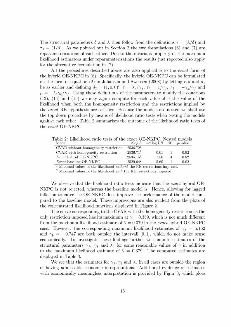
Table 2: Likelihood ratio tests of the exact OE-NKPC. Nested modelsModel 2 logL �2 logLR df. p-valueCVAR without homogeneity restriction 2536.721

CVAR with homogeneity restriction 2536.711 0.01 1 0.92Exact hybrid OE-NKPC 2535.152 1.56 4 0.82Exact baseline OE-NKPC 2529.642 5.60 1 0.021 Maximal values of the likelihood without the RE restrictions imposed.2 Maximal values of the likelihood with the RE restrictions imposed.

We observe that the likelihood ratio tests indicate that the exact hybrid OE-NKPC is not rejected, whereas the baseline model is. Hence, allowing for laggedin�ation to enter the OE-NKPC does improve the performance of the model com-pared to the baseline model. These impressions are also evident from the plots ofthe concentrated likelihood functions displayed in Figure 2.

The curve corresponding to the CVAR with the homogeneity restriction as theonly restriction imposed has its maximum at ̂ = 0:359, which is not much di¤erentfrom the maximum likelihood estimate of ̂ = 0:379 in the exact hybrid OE-NKPCcase. However, the corresponding maximum likelihood estimates of f = 5:162and b = �0:747 are both outside the intervall [0; 1], which do not make senseeconomically. To investigate these �ndings further we compute estimates of thestructural parameters f ; b and �h for some reasonable values of in additionto the maximum likelihood estimate of ̂ = 0:379. The computed estimates aredisplayed in Table 3.

We see that the estimates for f , b and �h in all cases are outside the regionof having admissable economic interpretations. Additional evidence of estimateswith economically meaningless interpretation is provided by Figur 3, which plots

15

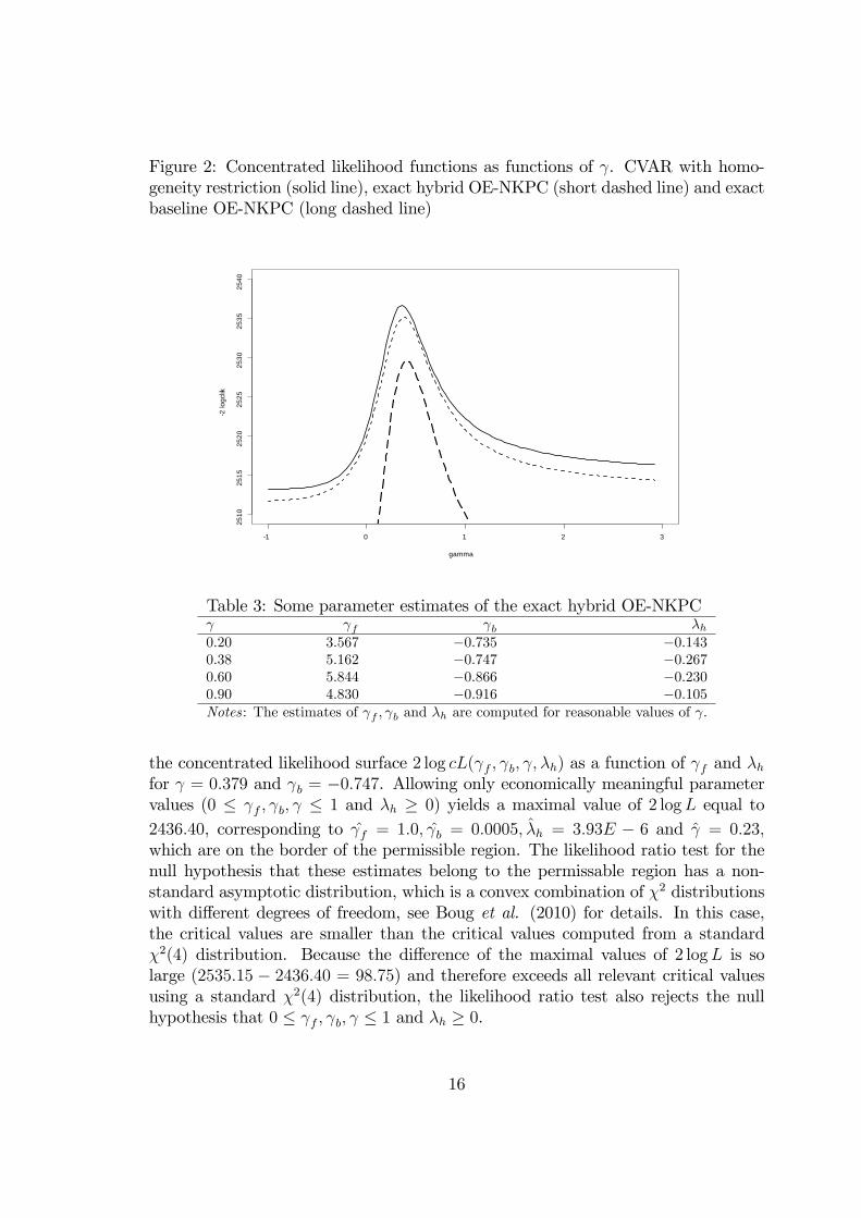
Figure 2: Concentrated likelihood functions as functions of . CVAR with homo-geneity restriction (solid line), exact hybrid OE-NKPC (short dashed line) and exactbaseline OE-NKPC (long dashed line)

­1 0 1 2 3

2510

2515

2520

2525

2530

2535

2540

gamma

­2 lo

gclik

Table 3: Some parameter estimates of the exact hybrid OE-NKPC f b �h0:20 3:567 �0:735 �0:1430:38 5:162 �0:747 �0:2670:60 5:844 �0:866 �0:2300:90 4:830 �0:916 �0:105Notes: The estimates of f ; b and �h are computed for reasonable values of :

the concentrated likelihood surface 2 log cL( f ; b; ; �h) as a function of f and �hfor = 0:379 and b = �0:747. Allowing only economically meaningful parametervalues (0 � f ; b; � 1 and �h � 0) yields a maximal value of 2 logL equal to2436:40, corresponding to ̂f = 1:0; ̂b = 0:0005; �̂h = 3:93E � 6 and ̂ = 0:23;which are on the border of the permissible region. The likelihood ratio test for thenull hypothesis that these estimates belong to the permissable region has a non-standard asymptotic distribution, which is a convex combination of �2 distributionswith di¤erent degrees of freedom, see Boug et al. (2010) for details. In this case,the critical values are smaller than the critical values computed from a standard�2(4) distribution. Because the di¤erence of the maximal values of 2 logL is solarge (2535:15 � 2436:40 = 98:75) and therefore exceeds all relevant critical valuesusing a standard �2(4) distribution, the likelihood ratio test also rejects the nullhypothesis that 0 � f ; b; � 1 and �h � 0.

16

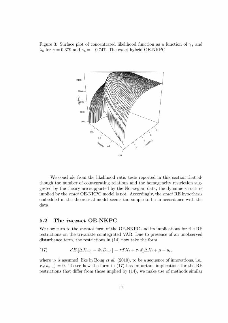
Figure 3: Surface plot of concentrated likelihood function as a function of f and�h for = 0:379 and b = �0:747. The exact hybrid OE-NKPC

gamma_f

2

4

6

8

lambda

­1.0

­0.5

0.0

0.5

­ 2log clik

1600

1800

2000

2200

2400

We conclude from the likelihood ratio tests reported in this section that al-though the number of cointegrating relations and the homogeneity restriction sug-gested by the theory are supported by the Norwegian data, the dynamic structureimplied by the exact OE-NKPC model is not. Accordingly, the exact RE hypothesisembedded in the theoretical model seems too simple to be in accordance with thedata.

5.2 The inexact OE-NKPCWe now turn to the inexact form of the OE-NKPC and its implications for the RErestrictions on the trivariate cointegrated VAR. Due to presence of an unobserveddisturbance term, the restrictions in (14) now take the form

(17) c0Et[�Xt+1 � �0Dt+1] = �d0Xt + � 1d

01�Xt + �+ ut;

where ut is assumed, like in Boug et al. (2010), to be a sequence of innovations, i.e.,Et(ut+1) = 0. To see how the form in (17) has important implications for the RErestrictions that di¤er from those implied by (14), we make use of methods similar

17

to those used by Boug et al. (2010) for bivariate VARs.7 First, the �tted reducedrank VAR may be written on level form as

(18) Xt = A1Xt�1 + A2Xt�2 + A3Xt�3 + �0Dt + �1 + �t;

and the restrictions in (17) correspondingly as

(19) c0Et[Xt+1 � �0Dt+1] = c00Xt + c

0�1Xt�1 + ut;

for c as earlier, c0 = c + �d + � 1d1 and c�1 = �� 1d1. Then, rewriting (19) at timet + 1, using the law of iterated expectations and inserting one-step ahead forecastsfrom the VAR, the following restrictions on the coe¢ cients of the VAR must besatis�ed in the inexact baseline OE-NKPC case when Et(ut+1) = 0:

c0(A21 + A2) + c00A1 + c

0�1 = 0(20)

c0(A1A2 + A3) + c00A2 = 0

c0(A1A3) + c00A3 = 0

(21) c0[A1(�0Dt+1 + �1) + �1] + c00(�0Dt+1 + �1) = 0:

The model (18) with reduced rank equal to unity contains 18 + 3 + 2 = 23 autore-gressive parameters in addition to the coe¢ cients of the deterministic terms. Thereare not more than 9 restrictions on the coe¢ cients of the VAR in (20), so usingthe reversed engineering approach of Kurmann (2007), expressing the likelihood interms of the parameters of the in�ation equation and the structural parameters �; and �, we end up with at least 17 freely varying parameters in addition to those from(21). However, the maximum likelihood estimates are computationally troublesometo obtain due to the rather complicated nature of the restrictions in (20), and isbeyond the scope of the present paper. To simplify matters, we therefore follow anumber of related studies and adopt the GMM approach to evaluate inexact versionsof the OE-NKPC.

The GMM approach in our context requires identifying relevant instrumentsand does not necessitate strong assumptions on the underlying model, as is the casewith the VAR and the likelihood based procedure used above. First, we de�ne inline with Galí and Gertler (1999) among others the RE forecast error as vt+1 ��pt+1 � Et�pt+1. Then, Et[vt+1] = 0 according to the RE hypothesis. ReplacingEt�pt+1 in (6) by its realised value �pt+1 we obtain the following modi�ed equationin the case of the inexact baseline OE-NKPC:

(22) �pt = ��pt+1 � �eqcmt + �t;

where �t = ut��vt+1 is a linear relationship between the stochastic error term ut andthe forecast error vt+1 in predicting future in�ation and the homogeneity restriction

7See also Kurmann (2007) and Fanelli (2008).

18

2 = 1 � 1 is satis�ed in eqcmt. We notice that estimating (22) by means of theerrors in variables method induces �rst order moving average errors by construction,see e.g. Bårdsen et al. (2005, p. 291) for details. Estimated serial correlation thuscorroborates forward-looking behaviour in the RE sense, but it may also be a signof model misspeci�cation, as discussed in Bårdsen et al. (2004). Nevertheless, thepossibility of serially correlated errors motivates the use of GMM. Under the REhypothesis in (6), we also have that

(23) Et f(�pt � ��pt+1 + �eqcmt)zt�1g = 0;

where zt�1 is a vector of instruments dated at time t � 1 and earlier. The orthog-onality conditions in (23) provide the basis for the GMM estimation of the inexactbaseline OE-NKPC in our context Because the instrument set includes only laggedvariables, we implicitly treat eqcmt as an endogenous variable.8 We use the corre-sponding GMM set up to estimate inexact versions of (7) and (8).

A potential shortcoming of our approach, as pointed out by e.g. Galí et al.(2005), is that GMM estimates may be biased in favour of �nding a signi�cantrole for expected future in�ation, even if that role is truly absent or negligible, ifthe instrument set includes variables that directly cause in�ation, but are omittedas regressors in the model speci�cation. Similarly, Mavroeidis (2005) argues thatNKPC models are likely to su¤er from underidenti�cation, and that identi�cation inempirical applications is achieved by con�ning important explanatory variables tothe set of instruments, with misspeci�cation as a result. In principle, misspeci�cationcan be tested using Hansen�s (1982) J test of overidentifying restrictions. However,Mavroeidis (2005) shows that using too many instruments seriously weaken thepower of the J test, thus obscuring speci�cation problems and distorting GMMbased inference. We address these issues below by using relatively few instrumentsthat may also play a role as additional explanatory variables.

Throughout the evaluation of (22) and the corresponding equations for (7) and(8), we use the following set of instruments similar to the predetermined variablesfrom the reduced rank VAR established above:

(24) zt�1 =

��pt�1;�pt�2;�pit�1;�pit�2;�ulct�1;

�ulct�2; eqcmt�1; �; SDit

�;

where � denotes a constant term.9 The number of instruments used in our analysesis small compared to e.g. Batini et al. (2005), who base their study on as much

8This could be justi�ed by the fact that pt = �pt + pt�1, and thus includes the left hand sidevariable as a right hand side variable in (22). It is common in the NKPC literature to use onlylagged instruments, see e.g. Galí and Gertler (1999) and Galí et al. (2001). One obvious reasonis that some current information may not be available at the date when price setters form theirexpectations.

9The impulse dummies D84Q1, D86Q3, D96Q1, D01Q3, D03Q1 and D03Q2 used in the VARto account for outliers and special events in the economy are not included in the set of instrumentsto facilitate GMM estimation in EViews6.

19

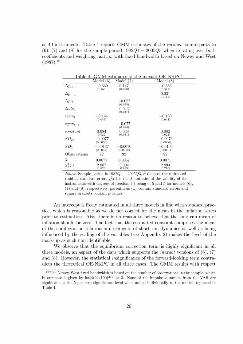
as 40 instruments. Table 4 reports GMM estimates of the inexact counterparts to(6), (7) and (8) for the sample period 1982Q4 � 2005Q3 when iterating over bothcoe¢ cients and weighting matrix, with �xed bandwidth based on Newey and West(1987).10

Table 4: GMM estimates of the inexact OE-NKPCModel (6) Model (7) Model (8)

�pt+1 �0:639(0:390)

0:147(0:220)

�0:636(0:385)

�pt�1 0:031(0:115)

�pit �0:027(0:075)

�ulct 0:043(0:017)

eqcmt �0:164(0:043)

�0:160(0:044)

eqcmt�1 �0:077(0:024)

constant 0:084(0:022)

0:039(0:011)

0:082(0:022)

SD2t �0:0077(0:0036)

�0:0076(0:0036)

SD3t �0:0137(0:0031)

�0:0070(0:0010)

�0:0136(0:0031)

Observations 92 92 92^� 0:0071 0:0057 0:0071�2J(�) 2:887

[0:823]3:004[0:699]

2:894[0:716]

Notes: Sample period is 1982Q4� 2005Q3, ^� denotes the estimatedresidual standard error, �2J(�) is the J statistics of the validity of theinstruments with degrees of freedom (�) being 6, 5 and 5 for models (6),(7) and (8), respectively, parenthesis (..) contain standard errors andsquare brackets contain p-values.

An intercept is freely estimated in all three models in line with standard prac-tice, which is reasonable as we do not correct for the mean in the in�ation seriesprior to estimation. Also, there is no reason to believe that the long run mean ofin�ation should be zero. The fact that the estimated constant comprises the meanof the cointegration relationship, elements of short run dynamics as well as beingin�uenced by the scaling of the variables (see Appendix 2) makes the level of themark-up as such non identi�able.

We observe that the equilibrium correction term is highly signi�cant in allthree models, an aspect of the data which supports the inexact versions of (6), (7)and (8). However, the statistical insigni�cance of the forward-looking term contra-dicts the theoretical OE-NKPC in all three cases. The GMM results with respect

10The Newey-West �xed bandwidth is based on the number of observations in the sample, whichin our case is given by int[4(92=100)2=9] = 3. None of the impulse dummies from the VAR aresigni�cant at the 5 per cent signi�cance level when added individually to the models reported inTable 4.

20

to the forward-looking term, the equilibrium correction term,^� and the J statis-

tics are hardly a¤ected when comparing models (6) and (8), the latter estimatedby including the �rst lag of in�ation from the list of instruments as an additionalregressor in the model. We notice that �pt�1 is far from being signi�cant in model(8), which is also the case for all the other variables from the instrument set. Theargument of Mavroeidis (2005) that identi�cation of the NKPC is achieved by con-�ning important explanatory variables to the set of instrument does not seem to berelevant in our empirical case.

We conclude from the range of GMM estimates in this section that neitherthe inexact baseline nor the inexact hybrid OE-NKPC �t Norwegian data well.Accordingly, we claim that introducing a disturbance term to our model in the wayit is interpreted here is not important when evaluating the empirical performanceof the OE-NKPC. Our �ndings stand in sharp contrast to several existing studiesusing GMM, which present evidence that the NKPC is a good approximation ofin�ation dynamics in the US and Europe, cf. Galí and Gertler (1999), Galí et al.(2001) and Batini et al. (2005) to mention some few examples.

6 A competing model of in�ationThat the forward-looking term in the OE-NKPC is statistically insigni�cant mo-tivates us to evaluate empirically the dynamic backward-looking ICM model as acompeting model of in�ation. We recall from Section 2 that the dynamic backward-looking ICM model is nested by and is a special case of the OE-NKPC when theforward-looking term is excluded from the model. Hence, to the extent that ourdata set is able to discriminate between the two competing models of in�ation, weshould �nd a well-speci�ed dynamic backward-looking ICM model as judged byeconometric criteria. To establish such a model in this section, we shall rely on ageneral-to-speci�c modelling strategy using the autometrics procedure available inOxMetrics, see Doornik and Hendry (2009). The point of departure is the generalconditional model

�pt = � +

2Xi=1

'1;i�pt�i +

2Xi=0

'2;i�ulct�i +

2Xi=0

'3;i�pit�i + �eqcmt�1(25)

+�1SD1t + �2SD2t + �3SD3t + �1D84Q1 + �2D86Q3

+�3D96Q1 + �4D01Q3 + �5D03Q1 + �6D03Q2 + et;

which is justi�ed by the cointegration analysis and the reduced rank VAR estab-lished above, both in terms of the number of lags and the weak exogeneity testresults of pit and ulct, see Boswijk and Urbain (1997). The error term et in (25)is assumed to be white noise. Brie�y speaking, autometrics �rst tests the generalmodel for misspeci�cation to ensure data coherence. If data coherence is satis�ed,

21

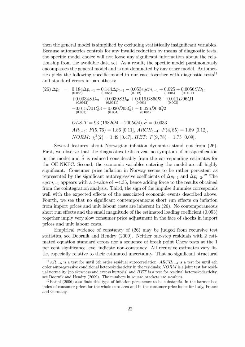
then the general model is simpli�ed by excluding statistically insigni�cant variables.Because autometrics controls for any invalid reduction by means of diagnostic tests,the speci�c model choice will not loose any signi�cant information about the rela-tionship from the available data set. As a result, the speci�c model parsimoniouslyencompasses the general model and is not dominated by any other model. Automet-rics picks the following speci�c model in our case together with diagnostic tests11

and standard errors in parenthesis:

�pt = 0:184(0:068)

�pt�1 + 0:144(0:065)

�pt�2 � 0:053(0:012)

eqcmt�1 + 0:025(0:005)

+ 0:0056(0:0011)

SD1t(26)

+0:0034(0:0012)

SD2t � 0:0039(0:0011)

SD3t + 0:019(0:003)

D86Q3� 0:011(0:003)

D96Q1

�0:015(0:003)

D01Q3 + 0:020(0:004)

D03Q1� 0:026(0:004)

D03Q2

OLS; T = 93 (1982Q4� 2005Q4); ^� = 0:0033AR1�5: F (5; 76) = 1:86 [0:11], ARCH1�4: F (4; 85) = 1:89 [0:12],

NORM : �2(2) = 1:49 [0:47], HET : F (9; 78) = 1:75 [0:09].

Several features about Norwegian in�ation dynamics stand out from (26).First, we observe that the diagnostics tests reveal no symptom of misspeci�cationin the model and

^� is reduced considerably from the corresponding estimates for

the OE-NKPC. Second, the economic variables entering the model are all highlysigni�cant. Consumer price in�ation in Norway seems to be rather persistent asrepresented by the signi�cant autoregressive coe¢ cients of �pt�1 and �pt�2.12 Theeqcmt�1 appears with a t-value of �4:35, hence adding force to the results obtainedfrom the cointegration analysis. Third, the sign of the impulse dummies correspondswell with the expected e¤ects of the associated economic events described above.Fourth, we see that no signi�cant contemporaneous short run e¤ects on in�ationfrom import prices and unit labour costs are inherent in (26). No contemporaneousshort run e¤ects and the small magnitude of the estimated loading coe¢ cient (0:053)together imply very slow consumer price adjustment in the face of shocks in importprices and unit labour costs.

Empirical evidence of constancy of (26) may be judged from recursive teststatistics, see Doornik and Hendry (2009). Neither one-step residuals with 2 esti-mated equation standard errors nor a sequence of break point Chow tests at the 1per cent signi�cance level indicate non-constancy. All recursive estimates vary lit-tle, especially relative to their estimated uncertainty. That no signi�cant structural11AR1�5 is a test for until 5th order residual autocorrelation; ARCH1�4 is a test for until 4th

order autoregressive conditional heteroskedasticity in the residuals; NORM is a joint test for resid-ual normality (no skewness and excess kurtosis) and HET is a test for residual heteroskedasticity,see Doornik and Hendry (2009). The numbers in square brackets are p-values.12Batini (2006) also �nds this type of in�ation persistence to be substantial in the harmonised

index of consumer prices for the whole euro area and in the consumer price index for Italy, Franceand Germany.

22

breaks are detected around the date of the shift in monetary policy regime fromexchange rate targeting to in�ation targeting (late March 2001) points to (26) notbeing subject to the Lucas critique.

Having identi�ed a well-speci�ed dynamic ICM model in-sample, we study theout-of-sample forecasting performance to shed light on its robustness with respectto relatively large movements in the exchange rate during the recent �nancial crisis,which took o¤ after the bankruptcy of Lehman Brothers September 15th 2008. Tay-lor (2000) argues that the extent to which a �rm matches exchange rate movementsby changing its own price depends on how persistent the movements are expected tobe. For a retail �rm that adds services to its imports of �nal goods, a depreciation ofthe exchange rate will raise the costs of the imports evaluated in domestic currency.If the depreciation is viewed as temporary, the retail �rm will according to Taylor(2000) pass through less of the depreciation to its own price.

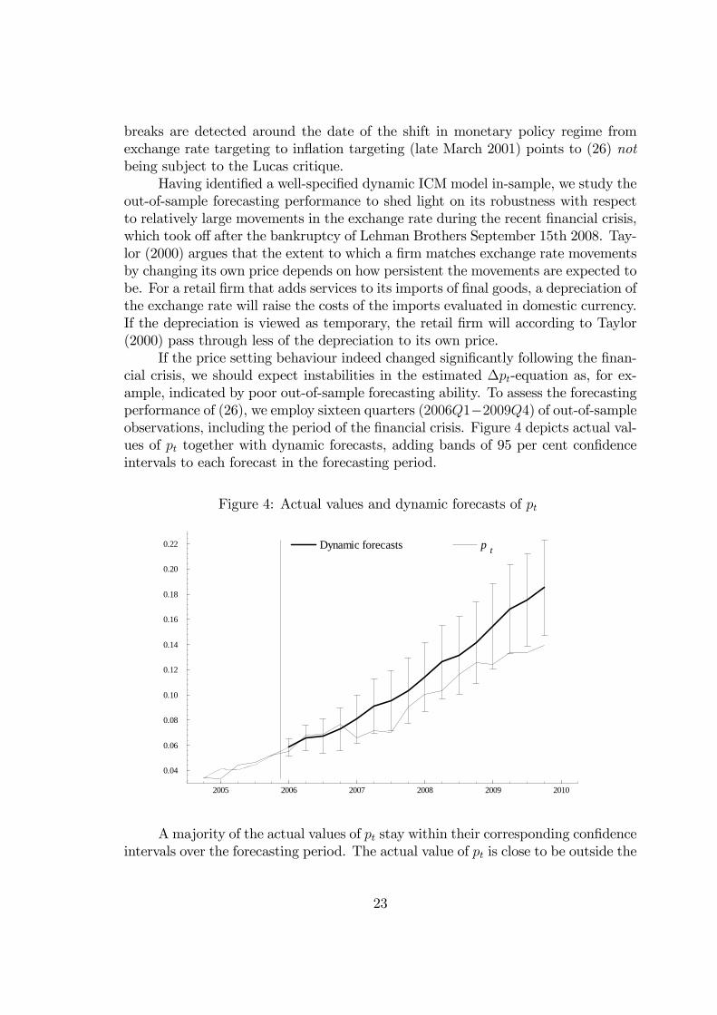
If the price setting behaviour indeed changed signi�cantly following the �nan-cial crisis, we should expect instabilities in the estimated �pt-equation as, for ex-ample, indicated by poor out-of-sample forecasting ability. To assess the forecastingperformance of (26), we employ sixteen quarters (2006Q1�2009Q4) of out-of-sampleobservations, including the period of the �nancial crisis. Figure 4 depicts actual val-ues of pt together with dynamic forecasts, adding bands of 95 per cent con�denceintervals to each forecast in the forecasting period.

Figure 4: Actual values and dynamic forecasts of pt

2005 2006 2007 2008 2009 2010

0.04

0.06

0.08

0.10

0.12

0.14

0.16

0.18

0.20

0.22 Dynamic forecasts p t

Amajority of the actual values of pt stay within their corresponding con�denceintervals over the forecasting period. The actual value of pt is close to be outside the

23

con�dence interval in the �rst quarter of 2007. The point in time in which the �rstsign of instability occurs does not, however, coincide with the period of the �nancialcrisis. Rather, the actual value of pt in 2007Q1 and the values thereafter are likelyto be in�uenced by the huge and transitory fall in electricity prices during the �rstquarter of 2007. Consequently, the dynamic forecasts overpredict the actual valuesof pt thereafter.

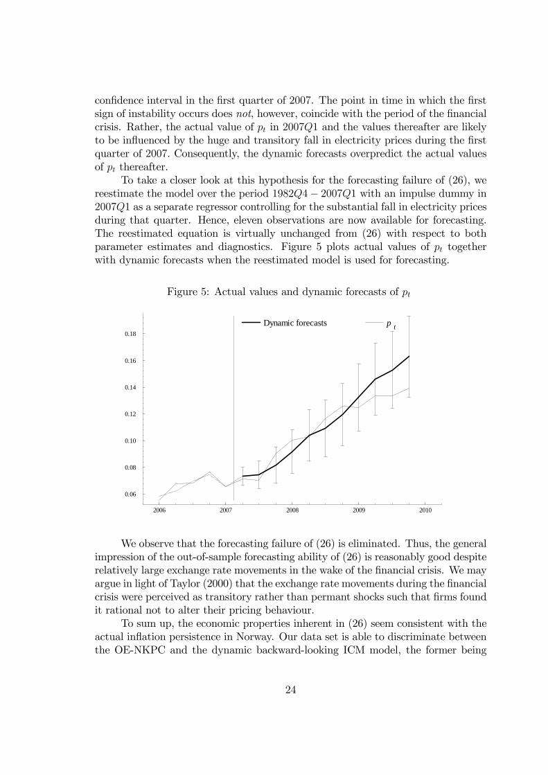
To take a closer look at this hypothesis for the forecasting failure of (26), wereestimate the model over the period 1982Q4� 2007Q1 with an impulse dummy in2007Q1 as a separate regressor controlling for the substantial fall in electricity pricesduring that quarter. Hence, eleven observations are now available for forecasting.The reestimated equation is virtually unchanged from (26) with respect to bothparameter estimates and diagnostics. Figure 5 plots actual values of pt togetherwith dynamic forecasts when the reestimated model is used for forecasting.

Figure 5: Actual values and dynamic forecasts of pt

2006 2007 2008 2009 2010

0.06

0.08

0.10

0.12

0.14

0.16

0.18Dynamic forecasts p t

We observe that the forecasting failure of (26) is eliminated. Thus, the generalimpression of the out-of-sample forecasting ability of (26) is reasonably good despiterelatively large exchange rate movements in the wake of the �nancial crisis. We mayargue in light of Taylor (2000) that the exchange rate movements during the �nancialcrisis were perceived as transitory rather than permant shocks such that �rms foundit rational not to alter their pricing behaviour.

To sum up, the economic properties inherent in (26) seem consistent with theactual in�ation persistence in Norway. Our data set is able to discriminate betweenthe OE-NKPC and the dynamic backward-looking ICM model, the former being

24

rejected in favour of the latter. Of course, relying on Bårdsen et al. (2005, p. 183),other and more elaborate dynamic backward-looking ICMmodels in which electricityprices and unemployment are allowed to play a role may exist. However, the purposehere has been to emphasise that discrimination between the two rival models ispossible through testable restrictions using the same information set throughout.

7 ConclusionsIn this paper, we have evaluated the empirical performance of an open economyversion of the NKPC (labelled OE-NKPC) as a model of Norwegian in�ation. Ourstarting point was the forward-looking linear quadratic adjustment cost model ofRotemberg (1982) and the theoretical principles of the incomplete competition model(ICM) for a small open economy. We showed that our OE-NKPC relates currentin�ation to expected future in�ation and the di¤erence between the actual priceand the price target in levels, a di¤erence being a theory consistent forcing variabledetermined by a weigthed average of unit labour costs and prices of total imports.The OE-NKPC thus includes variables both in levels and di¤erences that demandeconometric care with respect to both time series properties and cointegrated natureof these variables in the model. Such econometric issues have typically been ignoredin related studies on open economies data.

We �rst established by means of reduced rank regressions a cointegrating vec-tor between the price level and the target level in line with the ICM model andexisting evidence on Norwegian data. By way of contrast, we then found usingcointegrated VAR models and likelihood based testing procedures that the exactOE-NKPC, both in terms of the baseline and the hybrid version, does not receivemuch backing from the data. We obtained similar �ndings when various inexactOE-NKPC models were evaluated within the GMM framework. Accordingly, weclaim that introducing a disturbance term to the model in the way it is interpretedhere is not important when evaluating the empirical performance of the OE-NKPCas a model of Norwegian in�ation. Finally, we established a well-speci�ed dynamicICM model, which in addition to the theory consistent forcing variable includesbackward-looking terms only. We found that the dynamic ICM model encompassesthe OE-NKPC, is reasonably stable in-sample with a major monetary policy regimeshift from exchange rate targeting to in�ation targeting and forecasts well post-sample and during the recent �nancial crisis. All these �ndings are strong evidencein favour of the dynamic ICM model and the Lucas critique does not seem to beimportant in our empirical context. We conclude that including forward-lookingbehaviour when modelling consumer price in�ation in Norway seems unnecessary toarrive at a well-speci�ed model by econometric criteria.

25

References[1] Aukrust, O. (1977): In�ation in the Open Economy: A Norwegian Model,

in Worldwide In�ation, L.B. Krause and W.S. Salânt (eds.), Brookings, 1977,Washington D.C.

[2] Batini, N., B. Jackson and S. Nickell (2005): An Open Economy New KeynesianPhillips Curve for the UK, Journal of Monetary Economics 52, 1061-1071.

[3] Batini, N. (2006): Euro area in�ation persistence, Empirical Economics 31,977-1002.

[4] Bjørnstad, R. and R. Nymoen (2008): The New Keynesian Phillips CurveTested on OECD Panel Data, Economics. The Open-Access, Open-AssessmentE-Journal, Vol. 2, 2008-23, 1-18.

[5] Boswijk, H.P. and J-P Urbain (1997): Lagrange-multiplier tests for weak exo-geneity: A synthesis, Econometric Reviews 16, 21-38.

[6] Boug, P., Å. Cappelen and A. Rygh Swensen (2006): Expectations and RegimeRobustness in Price Formation: Evidence from Vector Autoregressive Modelsand Recursive Methods, Empirical Economics 31, 821-854.

[7] Boug, P., Å. Cappelen and A. Rygh Swensen (2010): The new KeynesianPhillips curve revisited, Journal of Economic Dynamics & Control 34, 858-874.

[8] Bårdsen, G., E.S. Jansen and R. Nymoen (2004): Econometric Evaluation ofthe New Keynesian Phillips Curve, Oxford Bulletin of Economics and Statistics66, Supplement, 671-686.

[9] Bårdsen, G., Ø. Eitrheim, E.S. Jansen and R. Nymoen (2005): The Economet-rics of Macroeconomic Modelling, Advanced Texts in Econometrics, OxfordUniversity Press, UK.

[10] Calvo, G.A. (1983): Staggered Prices in a Utility Maximising Framework, Jour-nal of Monetary Economics 12, 383-398.

[11] Doornik, J.A. (1998): Approximations to the Asymptotic Distribution of Coin-tegration Tests, Journal of Economic Surveys 12, 573-593.

[12] Doornik, J.A. and D.F. Hendry (2009): Empirical Econometric Modelling: Pc-Give 13, Volume I, Timberlake Consultants LTD, London.

[13] EViews6 (2007): User�s Guide, Quantitative Micro Software, LLC, UnitedStates of America.

26

[14] Fanelli, L. (2008): Testing the New Keynesian Phillips Curve through VectorAutoregressive Models: Results from the Euro area, Oxford Bulletin of Eco-nomics and Statistics 70, 53-66.

[15] Galí, J. and M. Gertler (1999): In�ation Dynamics: A Structural EconometricAnalysis, Journal of Monetary Economics 44, 195-222.

[16] Galí, J., M. Gertler and J.D. López-Salido (2001): European In�ation Dynam-ics, European Economic Review 45, 1237-1270.

[17] Galí, J., M. Gertler and J.D. López-Salido (2005): Robustness of the Estimatesof the Hybrid New Keynesian Phillips Curve, Journal of Monetary Economics52, 1107-1118.

[18] Gali, J. and T. Monacelli (2005): Monetary Policy and Exchange Rate Volatilityin a Small Open Economy, Review of Economic Studies 72, 707-734.

[19] Giordani, P. (2004): Evaluating New-Keynesian Models of a Small Open Econ-omy, Oxford Bulletin of Economics and Statistics 66, Supplement, 713-733.

[20] Gogley, T. and A.M. Sbordone (2008): Trend in�ation, indexation, and in�ationpersistence in the new Keynesian Phillips curve, American Economic Review98, 2101-2126.

[21] Guender, A.V. (2006): Stabilising properties of discretionary monetary policiesin a small open economy, The Economic Journal 116, 309-326.

[22] Guender, A.V. and Yu Xie (2007): Is there an exchange rate channel in theforward-looking Phillips curve? A theoretical and empirical investigation, NewZealand Economic Papers 41, 5-28.

[23] Hansen, L.P. (1982): Large Sample Properties of Generalized Method of Mo-ments Estimators, Econometrica 50, 1029-1054.

[24] Hansen, L.P. and T.J. Sargent (1991): Exact linear rational expectations mod-els: Speci�cation and estimation. In: Hansen, L.P., Sargent T.J. (Eds.), Ratio-nal Expectations Econometrics, Westview Press, Boulder.

[25] Hendry, D.F. (1995): Dynamic Econometrics, Oxford University Press, Oxford,England.

[26] Johansen, S. (1995): Likelihood-based Inference in Cointegrated Vector Au-toregressive Models, Advanced Texts in Econometrics, Oxford University Press,New York.

[27] Johansen, S. and A.R. Swensen (1999): Testing Exact Rational Expectations inCointegrated Vector Autoregressive Models, Journal of Econometrics 93, 73-91.

27

[28] Johansen, S. and A.R. Swensen (2004): More on Testing Exact Rational Ex-pectations in Cointegrated Vector Autoregressive Models: Restricted Constantand Linear Term, Econometrics Journal 7, 389-397.

[29] Johansen, S. and A.R. Swensen (2008): Exact Rational Expectations, Coin-tegration, and Reduced Rank Regression, Journal of Statistical Planning andInference 138, 2738-2748.

[30] Juillard, M., O. Kamenik, M. Kumhof and D. Laxton (2008): Optimal price set-ting and in�ation inertia in a rational expectation model, Journal of EconomicDynamics & Control 32, 2584-2621.

[31] Kara, A. and E. Nelson (2003): The exchange rate and in�ation in the UK,Scottish Journal of Political Economy 50, 585-608.

[32] Kurmann, A. (2007): VAR-based estimation of Euler equations with an appli-cation to New Keynesian pricing, Journal of Economic Dynamics & Control 31,767-796.

[33] Lindbeck, A. (ed.)(1979): In�ation and Employment in Open Economies, Am-sterdam, North- Holland.

[34] Mavroeidis, S. (2004): Weak Identi�cation of Forward-looking Models in Mon-etary Economics, Oxford Bulletin of Economics and Statistics 66, Supplement,609-635.

[35] Mavroeidis, S. (2005): Identi�cation Issues in Forward-looking Models Esti-mated by GMM, with an Application to the Phillips Curve, Journal of Money,Credit and Banking 37, 421-448.

[36] McCallum, B. and E. Nelson (1999): Nominal income targeting in an openeconomy optimising model, Journal of Monetary Economics 43, 553-578.

[37] Newey, W. and K. West (1987): A Simple Positive Semi-De�nite, Heteroskedas-ticity and Autocorrelation Consistent Covariance Matrix, Econometrica 55,703-708.

[38] R Development Core Team (2006): R: A language and environment for statis-tical computing, R Foundation for Statistical Computing, Vienna, Austria.

[39] Roberts, J.M. (1995): New-Keynesian Economics and the Phillips Curve, Jour-nal of Money, Credit and Banking 27, 975-984.

[40] Rotemberg, J.J. (1982): Sticky Prices in the United States, Journal of PoliticalEconomy 62, 1187-1211.

28

[41] Sbordone, A.M. (2005): Do Expected Future Marginal Costs Drive In�ationDynamics?, Journal of Monetary Economics 52, 1183-1197.

[42] Smets, F. and R. Wouters (2002): Openness, Imperfect Exchange Rate Pass-Through and Monetary Policy, Journal of Monetary Economics 49, 947-981.

[43] Svensson, L.E.O. (2000): Open-economy in�ation targeting, Journal of Inter-national Economics 50, 155-183.

[44] Taylor, J.B. (1979): Staggered wage setting in a macro model, American Eco-nomic Review 69, 108-113.

[45] Taylor, J.B. (1980): Aggregate dynamics and staggered contracts, Journal ofPolitical Economy 88, 1-23.

[46] Taylor, J.B. (2000): Low in�ation, pass-through, and the pricing power of �rms,European Economic Review, 44, 1389-1408.

[47] Tillmann, P. (2009): The New Keynesian Phillips curve in Europe: does it �tor does it fail?, Empirical Economics 37, 463-473.

29

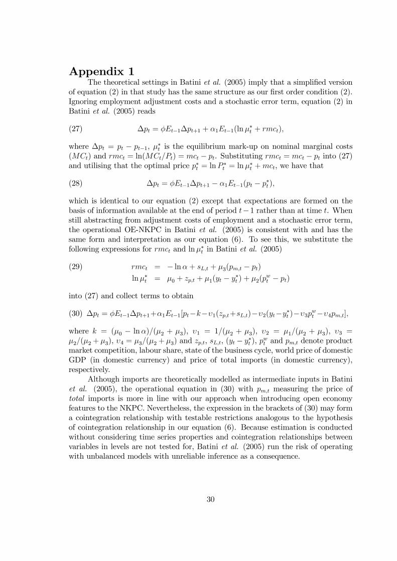
Appendix 1The theoretical settings in Batini et al. (2005) imply that a simpli�ed version

of equation (2) in that study has the same structure as our �rst order condition (2).Ignoring employment adjustment costs and a stochastic error term, equation (2) inBatini et al. (2005) reads

(27) �pt = �Et�1�pt+1 + �1Et�1(ln��t + rmct);

where �pt = pt � pt�1, ��t is the equilibrium mark-up on nominal marginal costs(MCt) and rmct = ln(MCt=Pt) = mct � pt. Substituting rmct = mct � pt into (27)and utilising that the optimal price p�t = lnP

�t = ln�

�t +mct, we have that

(28) �pt = �Et�1�pt+1 � �1Et�1(pt � p�t );

which is identical to our equation (2) except that expectations are formed on thebasis of information available at the end of period t�1 rather than at time t. Whenstill abstracting from adjustment costs of employment and a stochastic error term,the operational OE-NKPC in Batini et al. (2005) is consistent with and has thesame form and interpretation as our equation (6). To see this, we substitute thefollowing expressions for rmct and ln��t in Batini et al. (2005)

rmct = � ln�+ sL;t + �3(pm;t � pt)(29)

ln��t = �0 + zp;t + �1(yt � y�t ) + �2(pwt � pt)

into (27) and collect terms to obtain

(30) �pt = �Et�1�pt+1+�1Et�1[pt�k��1(zp;t+sL;t)��2(yt�y�t )��3pwt ��4pm;t];

where k = (�0 � ln�)=(�2 + �3), �1 = 1=(�2 + �3), �2 = �1=(�2 + �3), �3 =�2=(�2 + �3), �4 = �3=(�2 + �3) and zp;t, sL;t, (yt � y�t ), pwt and pm;t denote productmarket competition, labour share, state of the business cycle, world price of domesticGDP (in domestic currency) and price of total imports (in domestic currency),respectively.

Although imports are theoretically modelled as intermediate inputs in Batiniet al. (2005), the operational equation in (30) with pm;t measuring the price oftotal imports is more in line with our approach when introducing open economyfeatures to the NKPC. Nevertheless, the expression in the brackets of (30) may forma cointegration relationship with testable restrictions analogous to the hypothesisof cointegration relationship in our equation (6). Because estimation is conductedwithout considering time series properties and cointegration relationships betweenvariables in levels are not tested for, Batini et al. (2005) run the risk of operatingwith unbalanced models with unreliable inference as a consequence.

30

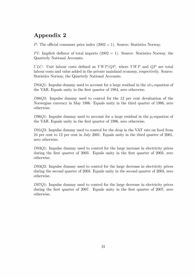
Appendix 2

P : The o¢ cial consumer price index (2002 = 1). Source: Statistics Norway.

PI: Implicit de�ator of total imports (2002 = 1). Source: Statistics Norway, theQuarterly National Accounts.

ULC: Unit labour costs de�ned as YWP=QP , where YWP and QP are totallabour costs and value added in the private mainland economy, respectively. Source:Statistics Norway, the Quarterly National Accounts.

D84Q1: Impulse dummy used to account for a large residual in the ulct-equation ofthe VAR. Equals unity in the �rst quarter of 1984, zero otherwise.

D86Q3: Impulse dummy used to control for the 12 per cent devaluation of theNorwegian currency in May 1986. Equals unity in the third quarter of 1986, zerootherwise.

D96Q1: Impulse dummy used to account for a large residual in the pt-equation ofthe VAR. Equals unity in the �rst quarter of 1996, zero otherwise.

D01Q3: Impulse dummy used to control for the drop in the VAT rate on food from24 per cent to 12 per cent in July 2001. Equals unity in the third quarter of 2001,zero otherwise.

D03Q1: Impulse dummy used to control for the large increase in electricity pricesduring the �rst quarter of 2003. Equals unity in the �rst quarter of 2003, zerootherwise.

D03Q2: Impulse dummy used to control for the large decrease in electricity pricesduring the second quarter of 2003. Equals unity in the second quarter of 2003, zerootherwise.

D07Q1: Impulse dummy used to control for the large decrease in electricity pricesduring the �rst quarter of 2007. Equals unity in the �rst quarter of 2007, zerootherwise.

31