Identifying the New Keynesian Phillips...

Identifying the New Keynesian Phillips Curve

James M. Nason and Gregor W. Smith†

First draft: May 2003August 2006

AbstractPhillips curves are central to discussions of inflation dynamics and monetary policy.The hybrid new Keynesian Phillips curve (NKPC) describes how past inflation, expectedfuture inflation, and a measure of real aggregate demand drive the current inflationrate. This paper studies the (potential) weak identification of the NKPC under GMM andtraces this syndrome to a lack of persistence in either exogenous variables or shocks.We employ analytic methods to understand the economics of the NKPC identificationproblem in the canonical three-equation, new Keynesian model. Given U.S., U.K., andCanadian data, we revisit the empirical evidence and construct tests and confidenceintervals based on the exact and pivotal Anderson and Rubin (1949) statistic that isrobust to weak identification. We also apply the Guggenberger and Smith (2006) LMtest to the underlying NKPC pricing parameters. Both tests yield little evidence offorward-looking inflation dynamics.

JEL classification: E31; C32.

Keywords: Phillips curve, Keynesian, identification, inflation.

†J.M. Nason: Research Department, Federal Reserve Bank of Atlanta; [email protected]. Smith: Department of Economics, Queen’s University; [email protected]

We thank the Social Sciences and Humanities Research Council of Canada and the Bank ofCanada Research Fellowship programme for support of this research. Smith thanks the Re-search Department of the Federal Reserve Bank of Atlanta for providing the environment forthis research. Richard Luger and Katharine Neiss provided data for Canada and the U.K. respec-tively, while Nikolay Gospodinov and Amir Yaron shared their code. Helpful comments wereprovided by Fabio Canova, Richard Clarida, Jean-Marie Dufour, Roger Farmer, Jon Faust, JeffreyFuhrer, Allan Gregory, Eric Leeper, Jesper Linde, Thomas Lubik, Antonio Moreno, Charles Nel-son, Michel Normandin, Athanasios Orphanides, Adrian Pagan, Juan Rubio-Ramırez, ThomasSargent, Christoph Schleicher, Michael Woodford, Jonathan Wright, Tao Zha, and seminar par-ticipants at the Canadian Economics Association meetings, Federal Reserve Bank of Atlanta,European Central Bank’s 3rd Workshop on Forecasting Techniques, Bank of Canada/UBC/SFUMacroeconomics Workshop, Queen’s University, University of Western Ontario Monetary Eco-nomics Conference, University of New South Wales, Johns Hopkins University, Vanderbilt Uni-versity, Duke University, North Carolina State University, the Federal Reserve Board, the ReserveBank of New Zealand, and the 2005 Econometric Society World Congress. The views in this pa-per represent those of the authors alone and are not those of the Bank of Canada, the FederalReserve Bank of Atlanta, the Federal Reserve System, or any of its staff.

USC FBE DEPT. MACROECONOMICS

presented by James NasonFRIDAY, Oct. 6, 20063:30 pm – 5:00 pm, Room: HOH-601K

& INTERNATIONAL FINANCE WORKSHOP

1. Introduction

Recent years have witnessed a boom in work on the Phillips curve. For a student

of monetary policy and the business cycle steeped in dynamic general equilibrium

methods, the revival of Phillips curve research might come as a shock. The shock

might be mitigated because the Phillips curve revival features debates on the role of

backward- and forward-looking expectations for inflation, on which measure of real

aggregate demand most directly influences inflation, on the response of monetary

policy to various disturbances, on the costs of disinflation, and on optimal monetary

policy. These debates often are framed by the new Keynesian Phillips curve (NKPC)

because it appears to provide a tent under which many views of inflation dynamics

can exist. However, whether to be inside or outside the Phillips curve revival tent

depends on the NKPC being a persuasive description of inflation dynamics.

Variations on the NKPC are just about limitless. The canonical NKPC is driven

either by current real marginal cost or today’s output gap and is forward-looking in

the current expectation of tomorrow’s inflation. Galı and Gertler (1999) add lagged

inflation to create a ‘hybrid NKPC’, which they use to address aspects of the debate

among Phillips curve revivalists. Specification of the NKPC has important implications

for monetary policy, and in particular for how central banks should react to real events

while maintaining inflation targets. Although contributions to this research are too

numerous to list, besides Galı and Gertler (1999), Fuhrer and Moore (1995), Roberts

(1995), and Sbordone (2002) make important empirical contributions. Theory and

evidence about the NKPC also are reviewed by Woodford (2003).

The hybrid NKPC is a second-order, linear, expectational difference equation.

Hansen and Sargent (1980) and Sargent (1987) study the dynamic and time series prop-

erties of this general class of stochastic models. Much empirical work on the NKPC

estimates it using instrumental variables (IV) methods, as Galı and Gertler (1999) do.

Generally, NKPC parameters prove difficult to pin down even with large instrument

sets. This suggests weak identification. Other symptoms of this syndrome include

instability of estimates across instrument sets, estimates which may approach those

1

from ordinary least-squares and hence be inconsistent, and Wald tests with size dis-

tortions. The goals of this paper are (a) to study the economics underlying weak

identification, with a view to drawing lessons and recommendations for applied work

and (b) to provide new tests of the NKPC that are robust to weak identification.

Section 2 provides background on the NKPC and begins our study of the eco-

nomics of weak identification. It shows that identification requires predictability of

future marginal cost or the output gap beyond that provided by current marginal cost

or current or lagged inflation. This predictability requires higher-order dynamics in

marginal cost, or additional instruments beyond lags of the variables in the NKPC.

Section 3 briefly considers a variety of approaches that have been proposed for

dealing with the identification problem, while using standard tools of GMM estimation

and testing. For example, some researchers have suggested calibrating the discount

factor in the Calvo pricing model, focusing on the purely forward-looking NKPC, or

indexing with lagged inflation. We note that some of these methods can improve

identification, but at the cost of precluding tests of the general, hybrid NKPC.

Section 4 details the GMM identification problem when the hybrid NKPC is set in a

typical, three-equation, new Keynesian model. The hybrid NKPC cannot be identified

under IV estimation in the baseline version of this model. For the hybrid NKPC to be

identified requires that either (a) one of the shocks to the system is persistent or (b) the

interest-rate rule involves a lagged interest rate (interest-rate smoothing). Studying

the NKPC within the three-equation, new Keynesian model thus does not generally

suggest added instruments that could aid identification. The key analytic results are

summarized in table 1.

Given these analytical results, section 5 therefore provides tests of the NKPC that

are robust to weak identification. We estimate the hybrid NKPC for the U.S., U.K., and

Canada, using a range of instruments. We first use the Anderson and Rubin (1949)

statistic to test the hybrid NKPC. This test is exact and robust to weak or omitted

instruments. Its application yields little evidence of forward-looking inflation dynam-

ics for the U.S. and U.K., but cannot reject the forward-looking NKPC for Canada. We

2

also apply the methods of Guggenberger and Smith (2006), which allow more power-

ful tests – again robust to weak identification – of the Calvo pricing parameters that

underlie the NKPC. These methods too yield little evidence in support of the hybrid

NKPC for the U.S., U.K., and Canada.

2. Background

A variety of pricing environments give rise to a hybrid NKPC that describes infla-

tion, πt :

πt = γfEtπt+1 + γbπt−1 + λxt, (1)

where we use xt to denote real aggregate demand (either real marginal cost or an out-

put gap). The studies by Rotemberg (1982), Roberts (1997), Fuhrer and Moore (1995),

and Galı and Gertler (1999) contain examples of these environments. The underlying

pricing behavior can range from smooth adjustment with quadratic costs to a varia-

tion of Calvo’s contract model (with or without firm-specific capital) in which some

price-setters are backward-looking. The hybrid NKPC (1) also may be consistent with

the dynamic indexing model suggested by Woodford (2003), assuming it is written in

the quasi-difference or change in inflation rather than the level.

An influential example of an environment underlying the NKPC is Calvo’s pricing

model. There the discount factor is β. A fraction θ of firms are allowed to change

prices each period. In Galı and Gertler’s hybrid version of the model, meanwhile, a

fraction ω are able to change prices but choose not to. Define φ = θ +ω[1 − θ(1 −β)]. Then the mapping between these structural paramaters and the reduced-form

parameters is:

γf = βθφ , γb = ωφ , λ = (1−ω)(1− θ)(1− βθ)φ

. (2)

This mapping is unique when the structural parameters are positive fractions.

It is often convenient to work with the general problem of identifying the parame-

ters γf , γb, and λ. In this case the environment is linear, so there is no distinction be-

tween local and global identification. Throughout the paper we also assume (with one

3

exception) that the roots of relevant difference equations imply stability and unique-

ness of solutions, and that the difference equation (1) follows from a pricing model

– in which all three parameters are positive – and not an observationally equivalent

environment, as in Beyer and Farmer (2004).

The hybrid NKPC (1) is a linear, second-order, stochastic difference equation. Our

study draws on tools for formulating these problems under rational expectations de-

veloped by Hansen and Sargent (1980) and Sargent (1987). We also draw on studies

of estimation in the linear-quadratic model by Gregory, Pagan, and Smith (1993), West

and Wilcox (1994), and Fuhrer, Moore, and Schuh (1995).

GMM estimation of the hybrid NKPC (1) uses sample versions of:

E[πt − γfπt+1 − γbπt−1 − λxt|zt

] = 0, (3)

and instruments zt . Given moment conditions (3), a necessary condition for identi-

fication of {γb, γf , λ} is that there are as many valid instruments as parameters (or

variables that explain inflation in this linear model). A test based on over-identification

requires at least four instruments or four such pieces of information. The instruments

must be uncorrelated with the GMM residuals, which are essentially forecast errors.

This is the order condition. Of course, being dated t − 1 or earlier is not sufficient

for an instrument to be valid: it must possess incremental information about πt+1.

The matrix of cross-products of the instruments and the right-hand-side variables in

the hybrid NKPC cannot be singular. This is the rank or ‘relevance’ condition of IV

estimation. We have omitted constant terms, as if the data have been demeaned. Of

course, if in applications a constant term is included in the NKPC, a vector of ones can

be used as an instrument while adding no net identifying information.

Identification obviously requires that one can predict πt+1 with at least one vari-

able other than πt , πt−1, and xt . This is a stringent requirement. Stock and Watson

(1999) report that few variables have power to forecast U.S. inflation during the great

disinflation of the 1980s and 1990s.

4

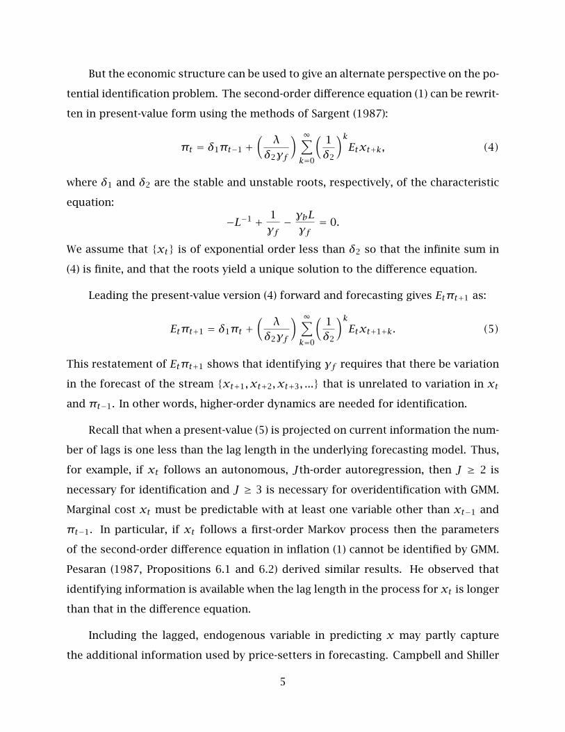
But the economic structure can be used to give an alternate perspective on the po-

tential identification problem. The second-order difference equation (1) can be rewrit-

ten in present-value form using the methods of Sargent (1987):

πt = δ1πt−1 +(λδ2γf

) ∞∑k=0

(1δ2

)kEtxt+k, (4)

where δ1 and δ2 are the stable and unstable roots, respectively, of the characteristic

equation:

−L−1 + 1γf− γbLγf

= 0.

We assume that {xt} is of exponential order less than δ2 so that the infinite sum in

(4) is finite, and that the roots yield a unique solution to the difference equation.

Leading the present-value version (4) forward and forecasting gives Etπt+1 as:

Etπt+1 = δ1πt +(λδ2γf

) ∞∑k=0

(1δ2

)kEtxt+1+k. (5)

This restatement of Etπt+1 shows that identifying γf requires that there be variation

in the forecast of the stream {xt+1, xt+2, xt+3, ...} that is unrelated to variation in xt

and πt−1. In other words, higher-order dynamics are needed for identification.

Recall that when a present-value (5) is projected on current information the num-

ber of lags is one less than the lag length in the underlying forecasting model. Thus,

for example, if xt follows an autonomous, Jth-order autoregression, then J ≥ 2 is

necessary for identification and J ≥ 3 is necessary for overidentification with GMM.

Marginal cost xt must be predictable with at least one variable other than xt−1 and

πt−1. In particular, if xt follows a first-order Markov process then the parameters

of the second-order difference equation in inflation (1) cannot be identified by GMM.

Pesaran (1987, Propositions 6.1 and 6.2) derived similar results. He observed that

identifying information is available when the lag length in the process for xt is longer

than that in the difference equation.

Including the lagged, endogenous variable in predicting x may partly capture

the additional information used by price-setters in forecasting. Campbell and Shiller

5

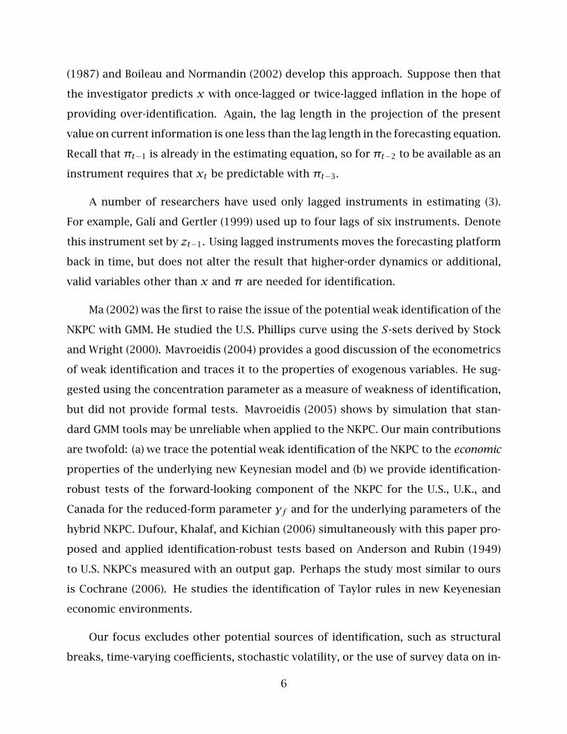
(1987) and Boileau and Normandin (2002) develop this approach. Suppose then that

the investigator predicts x with once-lagged or twice-lagged inflation in the hope of

providing over-identification. Again, the lag length in the projection of the present

value on current information is one less than the lag length in the forecasting equation.

Recall that πt−1 is already in the estimating equation, so for πt−2 to be available as an

instrument requires that xt be predictable with πt−3.

A number of researchers have used only lagged instruments in estimating (3).

For example, Galı and Gertler (1999) used up to four lags of six instruments. Denote

this instrument set by zt−1. Using lagged instruments moves the forecasting platform

back in time, but does not alter the result that higher-order dynamics or additional,

valid variables other than x and π are needed for identification.

Ma (2002) was the first to raise the issue of the potential weak identification of the

NKPC with GMM. He studied the U.S. Phillips curve using the S-sets derived by Stock

and Wright (2000). Mavroeidis (2004) provides a good discussion of the econometrics

of weak identification and traces it to the properties of exogenous variables. He sug-

gested using the concentration parameter as a measure of weakness of identification,

but did not provide formal tests. Mavroeidis (2005) shows by simulation that stan-

dard GMM tools may be unreliable when applied to the NKPC. Our main contributions

are twofold: (a) we trace the potential weak identification of the NKPC to the economic

properties of the underlying new Keynesian model and (b) we provide identification-

robust tests of the forward-looking component of the NKPC for the U.S., U.K., and

Canada for the reduced-form parameter γf and for the underlying parameters of the

hybrid NKPC. Dufour, Khalaf, and Kichian (2006) simultaneously with this paper pro-

posed and applied identification-robust tests based on Anderson and Rubin (1949)

to U.S. NKPCs measured with an output gap. Perhaps the study most similar to ours

is Cochrane (2006). He studies the identification of Taylor rules in new Keyenesian

economic environments.

Our focus excludes other potential sources of identification, such as structural

breaks, time-varying coefficients, stochastic volatility, or the use of survey data on in-

6

flation expectations. We also do not focus on the system estimator – where additional

identifying information is available from cross-equation and covariance restrictions.

Systems estimation has been studied by, among others, Fuhrer and Moore (1995),

Sbordone (2002, 2005), Kurmann (2005), Linde (2005), Jondeau and Le Bihan (2003),

and Fuhrer and Olivei (2004).

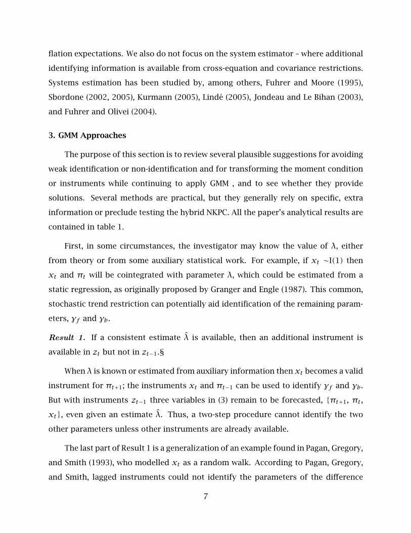
3. GMM Approaches

The purpose of this section is to review several plausible suggestions for avoiding

weak identification or non-identification and for transforming the moment condition

or instruments while continuing to apply GMM , and to see whether they provide

solutions. Several methods are practical, but they generally rely on specific, extra

information or preclude testing the hybrid NKPC. All the paper’s analytical results are

contained in table 1.

First, in some circumstances, the investigator may know the value of λ, either

from theory or from some auxiliary statistical work. For example, if xt ∼I(1) then

xt and πt will be cointegrated with parameter λ, which could be estimated from a

static regression, as originally proposed by Granger and Engle (1987). This common,

stochastic trend restriction can potentially aid identification of the remaining param-

eters, γf and γb.

Result 1. If a consistent estimate λ is available, then an additional instrument is

available in zt but not in zt−1.§

When λ is known or estimated from auxiliary information then xt becomes a valid

instrument for πt+1; the instruments xt and πt−1 can be used to identify γf and γb.

But with instruments zt−1 three variables in (3) remain to be forecasted, {πt+1, πt ,

xt}, even given an estimate λ. Thus, a two-step procedure cannot identify the two

other parameters unless other instruments are already available.

The last part of Result 1 is a generalization of an example found in Pagan, Gregory,

and Smith (1993), who modelled xt as a random walk. According to Pagan, Gregory,

and Smith, lagged instruments could not identify the parameters of the difference

7

equation without higher-order dynamics in the x-process. Result 1 also is relevant to

price-setting rules that are written in terms of the level of prices, rather than the in-

flation rate, because the price level is more likely to be nonstationary yet cointegrated

with the fundamental.

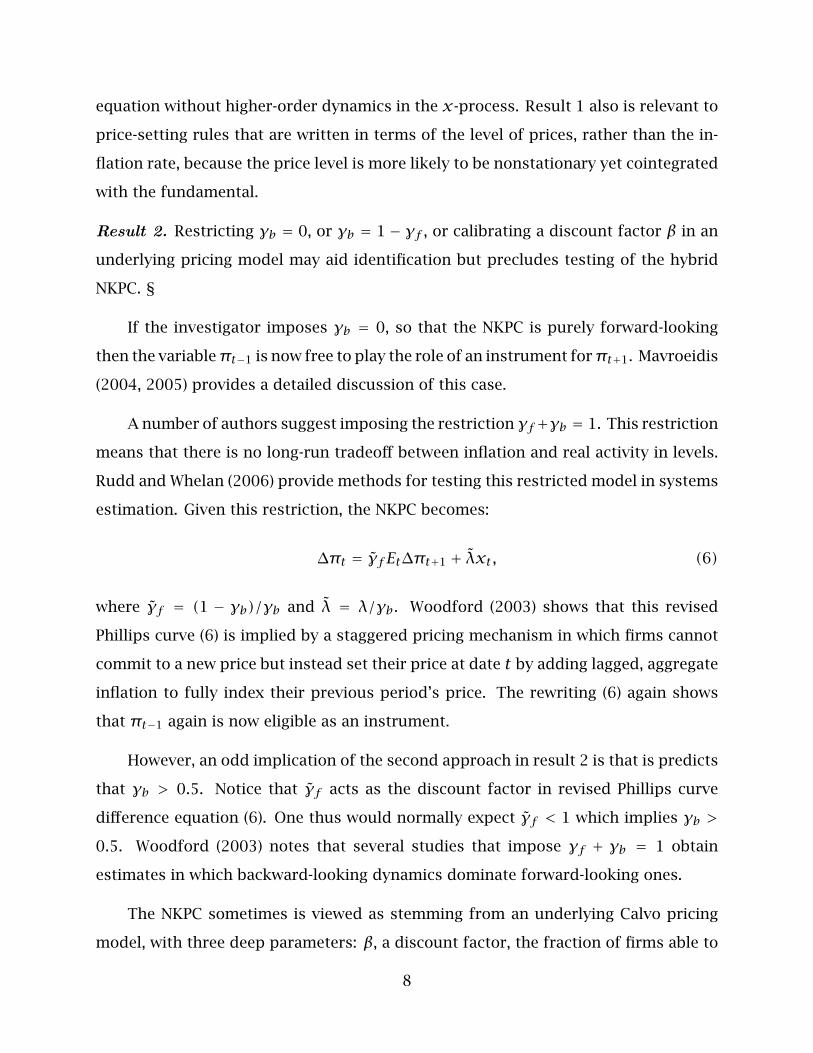
Result 2. Restricting γb = 0, or γb = 1− γf , or calibrating a discount factor β in an

underlying pricing model may aid identification but precludes testing of the hybrid

NKPC. §

If the investigator imposes γb = 0, so that the NKPC is purely forward-looking

then the variableπt−1 is now free to play the role of an instrument forπt+1. Mavroeidis

(2004, 2005) provides a detailed discussion of this case.

A number of authors suggest imposing the restriction γf+γb = 1. This restriction

means that there is no long-run tradeoff between inflation and real activity in levels.

Rudd and Whelan (2006) provide methods for testing this restricted model in systems

estimation. Given this restriction, the NKPC becomes:

∆πt = γf Et∆πt+1 + λxt, (6)

where γf = (1 − γb)/γb and λ = λ/γb. Woodford (2003) shows that this revised

Phillips curve (6) is implied by a staggered pricing mechanism in which firms cannot

commit to a new price but instead set their price at date t by adding lagged, aggregate

inflation to fully index their previous period’s price. The rewriting (6) again shows

that πt−1 again is now eligible as an instrument.

However, an odd implication of the second approach in result 2 is that is predicts

that γb > 0.5. Notice that γf acts as the discount factor in revised Phillips curve

difference equation (6). One thus would normally expect γf < 1 which implies γb >

0.5. Woodford (2003) notes that several studies that impose γf + γb = 1 obtain

estimates in which backward-looking dynamics dominate forward-looking ones.

The NKPC sometimes is viewed as stemming from an underlying Calvo pricing

model, with three deep parameters: β, a discount factor, the fraction of firms able to

8

change price, and the fraction able to change price that do not. Pre-setting β amounts

to setting γf conditional on γb and λ, and so it may allow identification.

An important corollary of result 2, however, is that naturally none of the restric-

tions in result 2 can be tested if the two remaining parameters are just identified. For

example, one cannot test the hybrid NKPC against the purely forward-looking one.

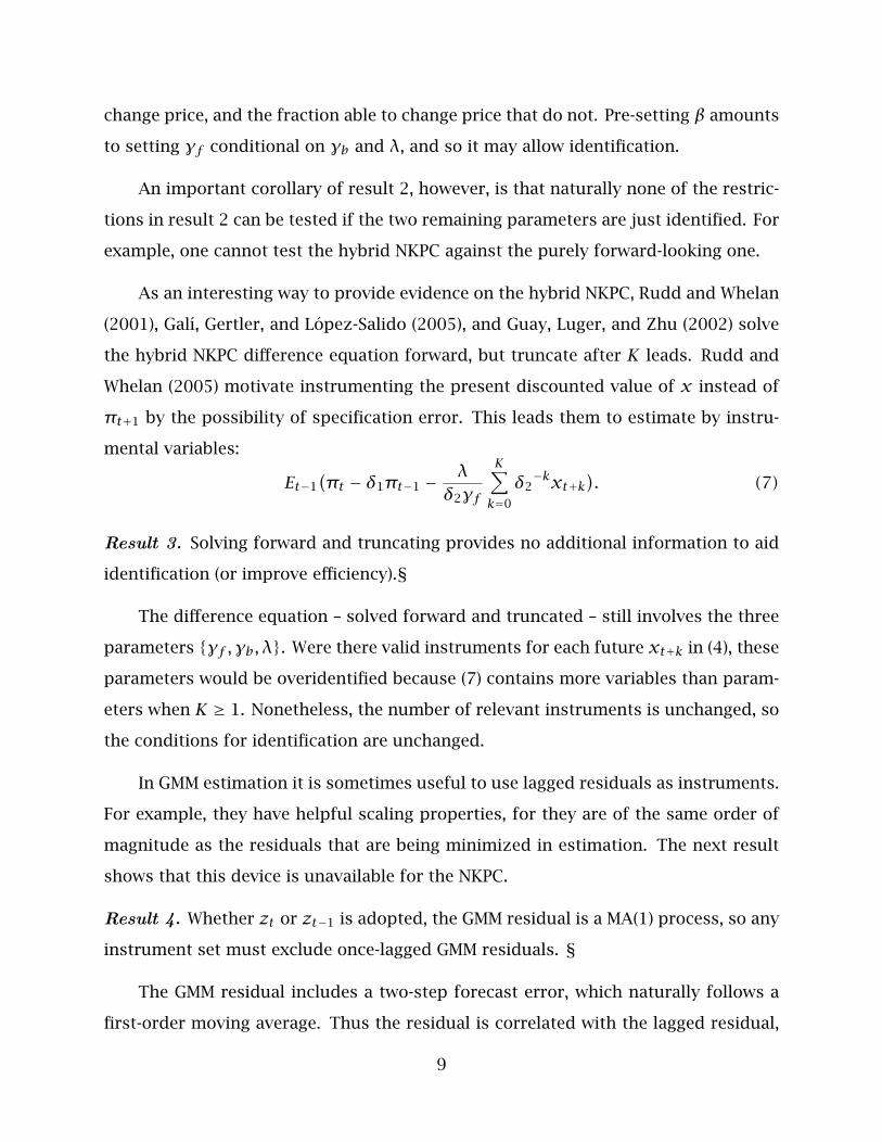
As an interesting way to provide evidence on the hybrid NKPC, Rudd and Whelan

(2001), Galı, Gertler, and Lopez-Salido (2005), and Guay, Luger, and Zhu (2002) solve

the hybrid NKPC difference equation forward, but truncate after K leads. Rudd and

Whelan (2005) motivate instrumenting the present discounted value of x instead of

πt+1 by the possibility of specification error. This leads them to estimate by instru-

mental variables:

Et−1(πt − δ1πt−1 − λ

δ2γf

K∑k=0

δ2−kxt+k

). (7)

Result 3. Solving forward and truncating provides no additional information to aid

identification (or improve efficiency).§

The difference equation – solved forward and truncated – still involves the three

parameters {γf , γb, λ}. Were there valid instruments for each future xt+k in (4), these

parameters would be overidentified because (7) contains more variables than param-

eters when K ≥ 1. Nonetheless, the number of relevant instruments is unchanged, so

the conditions for identification are unchanged.

In GMM estimation it is sometimes useful to use lagged residuals as instruments.

For example, they have helpful scaling properties, for they are of the same order of

magnitude as the residuals that are being minimized in estimation. The next result

shows that this device is unavailable for the NKPC.

Result 4. Whether zt or zt−1 is adopted, the GMM residual is a MA(1) process, so any

instrument set must exclude once-lagged GMM residuals. §

The GMM residual includes a two-step forecast error, which naturally follows a

first-order moving average. Thus the residual is correlated with the lagged residual,

9

which violates the orthogonality condition. However, this moving average can be ac-

counted for in constructing the weighting matrix in GMM estimation.

In summary, several methods suggested to ward off weak identification are prac-

tical, but they generally rule out testing of the hybrid NKPC. Thus identification and

testing requires higher-order dynamics or additional variables to predict inflation. A

natural question concerns the economic interpretation of these features. The next

section looks at their availability in a new Keynesian economic model.

4. Economic Sources of Weak Identification

Up to this point, we have discovered (or rediscovered) that identifying the hy-

brid NKPC depends on the multi-step predictability of the x-process. However, real

marginal cost or the output gap is endogenous in a dynamic, stochastic, general-

equilibrium model. We study identification in a more complete model in this section.

It seems natural to work with a typical, new Keynesian, trinity (i.e., three-equation)

model (NKTM) consisting of an NKPC, a linearized, dynamic IS schedule, and a Taylor

rule. Let y be the output gap and R be the central bank’s discount rate (the nominal

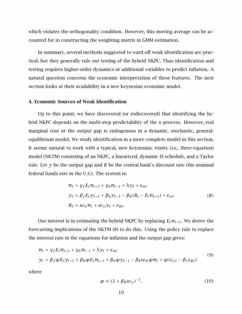
federal funds rate in the U.S.). The system is:

πt = γfEtπt+1 + γbπt−1 + λyt + επtyt = βfEtyt+1 + βbyt−1 − βR(Rt − Etπt+1)+ εytRt =ωππt +ωyyt + εRt.

(8)

Our interest is in estimating the hybrid NKPC by replacing Etπt+1. We derive the

forecasting implications of the NKTM (8) to do this. Using the policy rule to replace

the interest rate in the equations for inflation and the output gap gives:

πt = γfEtπt+1 + γbπt−1 + λyt + επtyt = βfϕEtyt+1 + βRϕEtπt+1 + βbϕyt−1 − βRωπϕπt +ϕ(εyt − βrεRt)

(9)

where

ϕ ≡ (1+ βRωy)−1. (10)

10

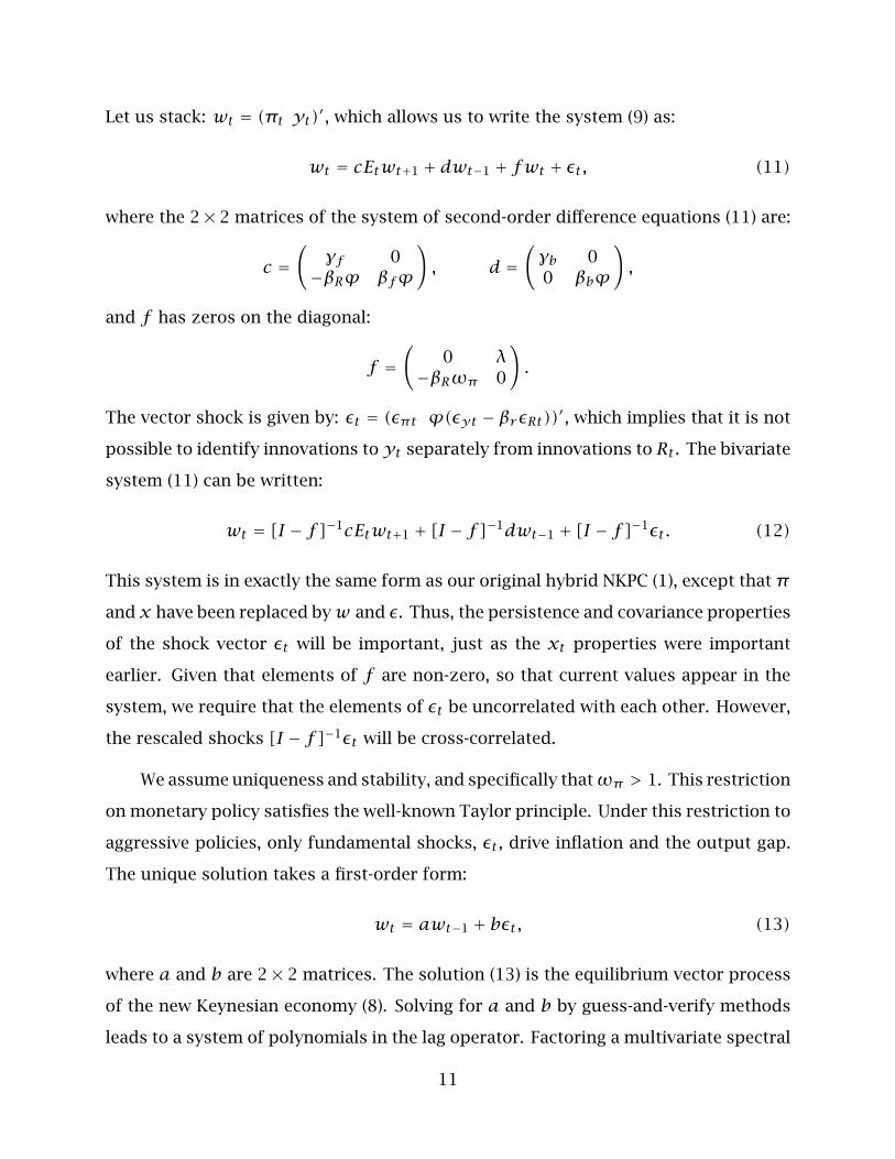
Let us stack: wt = (πt yt)′, which allows us to write the system (9) as:

wt = cEtwt+1 + dwt−1 + fwt + εt, (11)

where the 2× 2 matrices of the system of second-order difference equations (11) are:

c =(

γf 0−βRϕ βfϕ

), d =

(γb 00 βbϕ

),

and f has zeros on the diagonal:

f =(

0 λ−βRωπ 0

).

The vector shock is given by: εt = (επt ϕ(εyt − βrεRt))′, which implies that it is not

possible to identify innovations to yt separately from innovations to Rt . The bivariate

system (11) can be written:

wt = [I − f]−1cEtwt+1 + [I − f]−1dwt−1 + [I − f]−1εt. (12)

This system is in exactly the same form as our original hybrid NKPC (1), except that π

and x have been replaced byw and ε. Thus, the persistence and covariance properties

of the shock vector εt will be important, just as the xt properties were important

earlier. Given that elements of f are non-zero, so that current values appear in the

system, we require that the elements of εt be uncorrelated with each other. However,

the rescaled shocks [I − f]−1εt will be cross-correlated.

We assume uniqueness and stability, and specifically thatωπ > 1. This restriction

on monetary policy satisfies the well-known Taylor principle. Under this restriction to

aggressive policies, only fundamental shocks, εt , drive inflation and the output gap.

The unique solution takes a first-order form:

wt = awt−1 + bεt, (13)

where a and b are 2× 2 matrices. The solution (13) is the equilibrium vector process

of the new Keynesian economy (8). Solving for a and b by guess-and-verify methods

leads to a system of polynomials in the lag operator. Factoring a multivariate spectral

11

density matrix usually requires numerical methods; a and b cannot be found analyt-

ically in general. For discussion and examples, see Hansen and Sargent (1981) and

Sayed and Kailath (2001). Nonetheless, the form of the solution (13) tells us much

about the necessary conditions for identification.

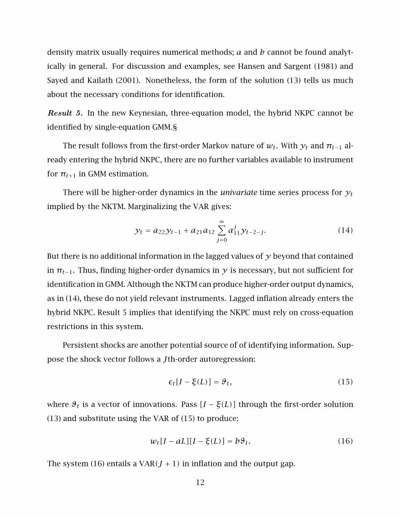
Result 5. In the new Keynesian, three-equation model, the hybrid NKPC cannot be

identified by single-equation GMM.§

The result follows from the first-order Markov nature of wt . With yt and πt−1 al-

ready entering the hybrid NKPC, there are no further variables available to instrument

for πt+1 in GMM estimation.

There will be higher-order dynamics in the univariate time series process for yt

implied by the NKTM. Marginalizing the VAR gives:

yt = a22yt−1 + a21a12

∞∑j=0

aj11yt−2−j. (14)

But there is no additional information in the lagged values of y beyond that contained

in πt−1. Thus, finding higher-order dynamics in y is necessary, but not sufficient for

identification in GMM. Although the NKTM can produce higher-order output dynamics,

as in (14), these do not yield relevant instruments. Lagged inflation already enters the

hybrid NKPC. Result 5 implies that identifying the NKPC must rely on cross-equation

restrictions in this system.

Persistent shocks are another potential source of of identifying information. Sup-

pose the shock vector follows a Jth-order autoregression:

εt[I − ξ(L)] = ϑt, (15)

where ϑt is a vector of innovations. Pass [I − ξ(L)] through the first-order solution

(13) and substitute using the VAR of (15) to produce:

wt[I − aL][I − ξ(L)] = bϑt. (16)

The system (16) entails a VAR(J + 1) in inflation and the output gap.

12

Result 6. One of the shocks to inflation, to the output gap, or to the interest rate

must be persistent for the hybrid NKPC to be identified by GMM in the NKTM (8).§

Identifying the second-order difference equation in inflation in GMM requires at

least second-order dynamics. A necessary condition for these dynamics to arise is

that the intrinsic, first-order dynamics of the NKTM (8) be augmented with first-order

dynamics in at least one shock. Given there are no zero elements in [I−f]−1, all three

shocks from the NKTM (8) affectπt . Thus, persistence in at least one shock is sufficient

for identification. Shock persistence also translates into serial correlation in inflation

and the output gap. This finding may help to explain the long lags in estimated NKTM

inflation and output gap equations reported, for example, by Linde (2005) and Jondeau

and Le Bihan (2003). Likewise, Ireland (2004) found that an autocorrelated cost shock

in the NKPC was necessary for empirical success of the NKTM.

There is an analogous result when the NKTM (8) possesses multiple equilibria.

Lubik and Schorfheide (2004) study a NKTM that associates the indeterminacy with

passive monetary policy, ωπ < 1, and sunspot (i.e. extrinsic) shocks. Under ωπ < 1,

they show that the rational expectations forecast of πt and yt is a first-order VAR

with forecast innovations a function of the fundamental shocks εt and the rational

expectation forecast errors, φt :

[I − τwL]Etwt+1 = τϑϑt + τφφt, (17)

where φt+1 = [yt+1−Etyt+1 πt+1−Etπt+1]′ and the τ matrices are functions of the

parameters of the NKTM. Given the linear NKTM (8), this class of passive monetary

policies also permits φt to be a linear function of εt and a vector of sunspot shocks,

ψt . It follows from these facts – Etwt+1 is the VAR(1) of (17) and φt depends on ψt ,

besides fundamental shocks – that wt becomes a (restricted) bivariate ARMA process

rather than a pure bivariate autoregression:

[I − µL]wt = κϑ[I − µθϑL]ϑt + κψ[I − µθψL]ψt, (18)

where µ denotes the stable eigenvalue of (17) and the κ and θ matrices are functions

of the NKTM parameters. Note that the first-order moving average of the bivariate

13

ARMA process (18) are functions of the fundamental and sunspot shocks. The econo-

metrician focuses on the sunspot to connect the observed data to one of the multiple

equilibria. This motivates Lubik and Schorfheide to argue that the sunspot shock in-

terpretation of indeterminacy (created byωπ < 1) explains serially correlated inflation

and output gap data.

Result 7. When the new Keynesian, three-equation model (8) possesses multiple equi-

libria and the rational expectations forecast errors are a (linear) function of the funda-

mental and extrinsic shocks, the GMM estimator of the hybrid NKPC is not identified.§

The key to Result 7 is that the lack of restrictions on the rational expectations

forecast errors under indeterminacy provides no additional identification information.

Although fundamental and sunspot shocks are news for an econometrician attempting

to estimate the NKTM (8), these shocks do not help forecast πt+1. However, this

approach to identifying the NKPC within a larger model imposes persistence and cross-

equation restrictions on the forecast innovation of the bivariate ARMA process (18) of

yt and πt , which can yield additional information for identification in the system.

The NKTM is a monetary model, in which the central bank’s policy tool is its

discount rate, Rt . Although our analysis of the NKPC with the NKTM uses the Taylor

rule to substitute for the discount rate in the dynamic IS schedule, it seems reasonable

to use Rt as an instrument.

Result 8. With the Taylor rule in the NKTM (8), the current, nominal, policy interest

rate, Rt is not a valid instrument in the NKPC.§

The nominal interest rate is a natural predictor of πt+1 and so might seem to

be a natural instrument. It is invalid because under the Taylor rule Rt is set as a

proportionωπ of the current inflation rate πt which in turn is the dependent variable

in the hybrid NKPC. The correlation between Rt and επt violates the order condition.

Result 9. Lagged policy interest rates are valid but inefficient instruments in the

NKTM.§

Recall that the solution (13) describes the optimal forecast of πt+1 in the NKTM

14

based on lags of inflation and the output gap. Meanwhile, inspection of the lagged

Taylor rule shows that the nominal interest rate contains information on the lagged

output gap and inflation but (a) with an error εR and (b) with Taylor-rule coefficients

on the lagged values of inflation and the output gap that will not correspond to the

elements of the optimal coefficient matrix a given in the solution (13).

Result 10. Interest-rate smoothing in monetary policy may provide an alternate

source of identification.§

There is much debate about whether the discount rate can be partly explained by

its own lag due to persistent shocks or to an interest rate smoothing policy. Suppose

the policy rule is:

Rt = (1− υ)(ωππt +ωyyt)+ υRt−1 + εRt (19)

with 0 < υ < 1. The current interest rate thus reflects information on the entire

history of inflation, the output gap, and policy shocks εRt . The output gap inherits

this memory because Rt enters the equation for the output gap in the NKTM (8).

Thus, additional instruments become available in the same way that Result 6 adds

them using shock persistence.

This section has focused on the bivariate VAR in {wt} implied by the NKTM (8)

because of our interest in instrumenting πt+1 in the hybrid NKPC. Thus, we have not

studied the complete reduced form, or addressed the identification of other NKTM

parameters. The main result of this section is that a persistent shock or an interest

rate smoothing policy is necessary for the hybrid NKPC to be identified by GMM within

the NKTM. Table 1 summarizes the results of this section.

5. Revisiting the Evidence: Robust Tests

The theory in section 4 suggests that candidate instruments may not be available

for GMM estimation of the NKPC, unless there are autocorrelated shocks or interest-

rate smoothing. Identifying the NKPC under GMM may be challenging. We thus turn

to tests of the NKPC that are valid even under weak identification. We draw inference

15

without using a system by using simple statistics from Anderson and Rubin (1949)

plus some recent developments. We next apply our results to the estimation and

testing of hybrid NKPCs for the U.S., U.K., and Canada. The data consists of GDP

inflation and measures of real marginal cost. The appendix describes the data sources.

5.1 Statistics

First, we study the time-series properties of xt . We estimate univariate autore-

gressions for xt , and test the lag length from J = 1 to J = 6 lags using a likelihood

ratio statistic, the AIC, and the SIC. Recall from section 2 that – if there are no instru-

ments other than lags of x – then J ≥ 2 is necessary for identification in GMM. We

next include lagged values of inflation and report the results of a pre-test of the null

hypothesis that {πt} does not Granger-cause {xt}. Section 2 also noted that finding

a role for lagged inflation in forecasting x suggests that further instruments may be

available. These could include lags of inflation beyond the first two or other variables

that lead to Granger-causality because of the superior information of price-setters.

Second, our main interest is in instrumental-variables estimation, so we estimate:

E[πt − γfπt+1 − γbπt−1 − λxt|zt] = 0 (20)

by GMM and report point estimates and standard errors as well as the J-test statistic

of over-identifying restrictions and its p-value. Following Result 4, GMM estimators

will allow for a first-order moving average in the GMM residual. The weighting matrix

will be the continuous-updating version introduced by Hansen, Heaton, and Yaron

(1996), which has good finite-sample properties and is invariant to the normalization

of the hybrid NKPC (1). Of course, these standard estimates and inferences may be

suspect due to weak identification but the idea is to show how conclusions may differ

between these methods and those that are robust to weak identification.

Third, we calculate Anderson-Rubin (1949) statistics to test several hypotheses,

and find the implied confidence intervals. Excellent surveys of inference under weak

identification are provided by Dufour (2003) and Andrews and Stock (2005). For the

just-identified case, the Anderson-Rubin test is preferred, according to these authors.

16

The statistics from GMM estimation (20) depend on nuisance parameters under weak

identification. In contrast, the AR statistics are pivotal in finite samples. To test

H0 : γf = γf0 one projects as follows:

πt − γf0πt+1 = α0 +α1πt−1 +α2xt +α3ut, (21)

with auxiliary variables ut , then constructs the Anderson-Rubin (AR) F -statistic for

H′0 : α3 = 0. The idea is that there should be no further role for ut at the true value

for γf . In our case, γf is a scalar. This yields a F(k + 2, T − k) statistic, where k + 2

is the total number of exogenous variables and instruments. The Anderson-Rubin

(AR) statistic provides an exact test, which is robust to (a) weak instruments and

(b) omitted instruments. We do not need all the u-elements necessarily, but power

is lower if irrelevant instruments are included. The test statistic also is robust to

misspecification of the forecasting rule for πt+1 (i.e., its size is not affected, though

again its power may be).

The distributional assumption underlying the statistic’s being pivotal in finite

samples is normality of the GMM residuals. In the literature, the main drawbacks to

this approach arise when the structural equation is non-linear, or when there is more

than one endogenous, explanatory variable and we want to study subsets of their

coefficients. But here the hybrid NKPC is linear, and γf is a scalar.

The AR statistics also can be used to construct confidence intervals. A confidence

set is:

C(α) = {γf0 : AR(γf0) ≤ Fα(k, T − k− 2)}. (22)

Since γf is a scalar, there is a quadratic solution, given by Zivot, Startz, and Nelson

(1998). The coefficients of the quadratic equation are functions of the data and the

F−statistic at significance level α and degrees of freedom dim(u) and T − 2 − k.

With over-identification this confidence set can be empty. Without identification, it

can be unbounded. More generally, Andrews and Stock (2005, p 18) describe how

this confidence interval may be conservative (too wide) if there are other endogenous

right-hand-side variables.

17

Fourth, one criticism of the Anderson-Rubin tests is that they lack power when

there is overidentification. We find these tests reject for the U.S. and U.K. data. Thus,

a lack of power is not a a central issue in this study. A variety of approaches have been

proposed recently to correct this potential shortfall. We apply the LM test of Guggen-

berger and Smith (2006), which is robust to weak instruments and suffers no power

loss as over-identification rises. Guggenberger and Smith (GS) also present Monte

Carlo work in which their LM statistic has good sampling properties. For example,

its power properties are comparable to the test of Kleibergen (2005), and sometimes

superior when there are many instruments. Thus our evidence complements Dufour,

Khalaf, and Kichian (2006) who apply Kleibergen’s test to the U.S. NKPC.

A further advantage of the GS LM statistic is that it allows tests of parameters from

nonlinear moment condition models. Recall that the NKPC interprets the parameters

{γf , γb, λ} as arising from an underlying structure with parameters {β,θ,ω} given

the mapping (2). We employ the GS LM statistic to test hypotheses on several values

of θ and ω. In this approach we assume that parameters not under test are strongly

identified. In test statistics, these parameters are replaced by consistent estimates.

For methods to test subsets of parameters under weak identification, also see Dufour

and Tamouti (2003), Guggenberger and Smith (2006, section 2.3), and section 7.8 of

Andrews and Stock (2005).

5.2 United States

Table 2 presents evidence on real marginal cost dynamics for a U.S. sample of

1949Q1 − 2001Q4. We fail to reject the null that inflation does not Granger-cause

real marginal cost according to the first two rows of table 2. In addition, the AIC and

LR statistic choose a lag length of 3, while the SIC selects a lag length of 1 for the

x-autoregression. It is not surprising then that the second-order coefficient in this

regression is insignificantly different from zero. The implication of these pre-tests is

that finding relevant instruments may be a challenge in the U.S. data. Although U.S.

real marginal cost is persistent (the half life of a shock is about seven quarters), there

is not strong evidence of higher-order dynamics in U.S. real marginal cost. Campbell

18

and Shiller (1987) and Boileau and Normandin (2002) also show that the presence of

other predictors of xt should lead to a role for lagged inflation, yet we find none here.

Thus, the quest for other instruments may not be fruitful.

Table 3 contains single-equation GMM estimates. Most of the work is done by the

instruments {πt−1, xt, xt−2}, as is suggested by the pre-test evidence that only xt and

xt−2 help forecast xt+1. Adding further instruments increases the precision slightly

but does not lead to significant changes in the estimates. The J-test clearly does not

reject the over-identifying restrictions.

The estimated weight attributed to backward-looking inflationary expectations,

γb, ranges from 0.28 to 0.42, depending on the instrument set. The GMM estimates

show these expectations are dominated by forward-looking expectations because γf

ranges from 0.52 to 0.70. The response of πt to xt , denoted λ, also takes plausible

values, between 0.1 and 0.9 percent, but is not statistically significant (for a five per-

cent test). Our results are comparable to those of Galı and Gertler (1999, table 2), but

we obtain smaller and insignificant estimates of λ using smaller instrument sets.

Table 3 includes estimates of {θ,ω,β} on the U.S. data. The estimates imply that

about 90 percent of firms have the opportunity to change price each quarter and of

those 30-55 percent choose not to do so. We also find reasonable estimates for the

discount factor β.

Next, we provide tests for the forward-looking component in the U.S. NKPC that

are robust to weak identification. Table 4 presents AR F -statistics and their associated

p-values based on equation (21) and a grid of potentially ‘true’ γf = γf0. We set γf0

to [0.0, 0.2, 0.5, 0.6, 0.7, 0.8, 0.9, 0.99]. The AR statistics in the first row reveal little

evidence against the null of γf = γf0, for any of these values of γf0 given ut = xt−2.

When we add instruments though – in the next two rows – we can reject any of the null

hypotheses at standard significance levels. Thus, lags of real marginal cost besides

xt−2 matter for predicting the quasi-difference of πt and πt+1. The test is correctly

sized even if these added instruments are weak, which gives us a formal rejection of

the forward looking model.

19

The asymptotic 95 percent confidence interval C(α = 0.05) of γf , given in (22),

reflects the evidence of table 4. The solution yields C(0.05) = {−6.75, 0.05},{0.60,0.84}, and {−0.10, 1.24} for ut = xt−2, {xt−1, xt−2}, and {xt−1, . . . , xt−4}, re-

spectively. The smallest (just-identified) and largest (overidentified) instrument sets

yield asymptotic 95 percent confidence intervals that contain zero. Only the informa-

tion vector with the first two lags of x produces a confidence interval with reasonable

values of γf .

These wide confidence intervals yield the same, negative conclusion as do the

large S-sets found by Ma (2002). It is interesting to note the contrast with some of

the findings of Dufour, Khalaf, and Kichian (2006) who use a real-time output gap

measure in the U.S. NKPC and cannot reject a significant, forward-looking component

in U.S. inflation using robust methods. It remains an open question how sensitive test

results are to the choice between using marginal cost or the output gap in the NKPC

or, indeed, to different ways of measuring these variables.

Table 5 presents the GS test statistics for various values of θ and, separately, of

ω. The grids for these underlying parameters are suggested by the GMM estimates

in table 3. Across a grid of values, the test rejects each value of θ with the exception

of θ = 0.9 on the just-identified instrument set, which yields an estimate of β greater

than one. When further instruments are added, this value too is rejected. With larger

instrument sets, the test also rejects each value of ω. For those ω that do not reject

the GS test, the estimates of θ are between 0.93 and 1.03. Joint tests (not shown but

available on request) lead to similar conclusions.

5.3 United Kingdom

The estimation sample for the U.K. is 1961Q1 − 2000Q4. Table 2 shows that

the Granger causality pre-test provides strong evidence of predictability in both di-

rections. This result implies that lagged values of inflation (beyond the first two lags)

may be available as instruments. The second set of pre-tests indicate a lag length

in the x-autoregression of J = 5 using the LR test and SIC. This places more of the

history of x in the instrument vector zt than in the U.S. case.

20

Table 6 contains estimates of the U.K. hybrid NKPC. The GMM estimates depend on

instrument choice. Once lags up to xt−4 are included, the coefficients accord with the-

ory and are estimated with some precision. However, the over-identifying restrictions

are rejected when xt is an instrument. When xt is not an instrument, the estimates

of γf , γb, and λ are significant at the ten percent level or better. Neiss and Nelson

(2002) obtain statistically significant estimates of λ, but use dummy variables to con-

trol for a variety of price shocks. Table 6 also shows that the Calvo parameters are

quite sensitive to the instrument set, a potential sign of weak identification.

In contrast with the standard methods in table 6, however, table 7 gives evidence

against the null of γf = γf0 for the U.K. hybrid NKPC. The significance levels of the

AR statistics average 0.03 in table 7, for the projection (21), on the same grid of values

of γf0 used for table 4. Only two of the 16 AR statistics have p-values that exceed ten

percent, which are associated with the instrument xt−1, and γf0 near unity.

The AR 95 percent asymptotic confidence interval (22) of γf is C(0.05) = {−0.87,

−0.01} when ut = xt−1, and C(0.05) = {0.02, 0.97} when ut = {xt−1, ..., xt−4}. Thus

the confidence interval of γf has the wrong sign with the smaller information set.

The confidence interval takes the correct sign using the larger information set and

matches values set for γf0 in table 7. Nonetheless, with equal probability γf runs

from economically meaningless values to values that reveal an important role for

forward-looking inflationary expectations.

Table 8 presents the GS test statistics. The results are even more negative than in

the U.S. case shown in table 5. The test rejects each value of θ orω that we investigate.

Overall, then, the methods that are robust to weak identification provide a different

impression of the U.K. NKPC than do standard methods.

5.4 Canada

Estimating and testing the Canadian NKPC uses data from 1963Q1 to 2000Q4.

Table 2 shows that Canadian inflation Granger-causes real marginal cost. This table

also shows real marginal cost fails to Granger-cause inflation – in contrast to results

21

for the U.K. and U.S. data. The pre-tests for lag length reveal a persistence pattern

similar to that in U.S. real marginal cost, according to the LR test, the AIC, and the

SIC. In the time series for {xt}, once-lagged costs play a large predictive role and

thrice-lagged costs play an additional role, that is statistically significant. However,

a half-life of 8.5 quarters with respect to a shock to its third-order, autoregressive

process shows that Canadian real marginal cost is more persistent than it is in the

U.K. and the U.S. data.

Table 9 contains estimates of the hybrid NKPC parameters γf , γb, and λ for

Canada. They suggest that the hybrid NKPC is poorly identified. For example, the

point estimates γf and γb are sensitive to the instrument set. When we include πt−2

as an instrument, these two coefficients are similar to those found in the U.S. data,

with a large role for future inflation. Guay, Luger, and Zhu (2003) estimate the hybrid

NKPC using a wider range of instruments. They increase precision and reject the over-

identifying restrictions. However, we reproduce their finding that λ is insignificant.

This indicates little role for real marginal cost in Canadian inflation dynamics. Table 9

also shows that either we cannot find an economically plausible value for the discount

factor β or we obtain a wide 95 percent asymptotic confidence interval for β that runs

from 0.71 to 1.24 (using the largest instrument vector).

Table 10 includes AR statistics that favor forward-looking inflation dynamics for

Canada, which is the opposite found in the U.S. and the U.K. data. None of the hy-

pothesized values of γf can be rejected at the five percent level in table 10. Thus,

the AR 95 percent asymptotic confidence intervals (22) for γf , C(0.05), should cover

plausible values. For instrument vectors ut = xt−2, {xt−1, xt−2}, and {xt−1, . . . , xt−4},C(0.05) = {−0.00, 0.97}, {−0.00, 0.78}, and {−0.00, 0.97}, respectively.

The non-rejection in table 10 may reflect a lack of test power. Table 11 presents

the GS test statistics for Canada. Recall that this test has greater power in over-

identified cases. With relatively small instrument sets, there is some support for the

selected values of θ or ω, but at these values the estimates of γf are less than 0.1.

But with larger instrument sets, all the values of θ and ω we condider are rejected.

22

Thus, the GS LM tests limit support for the hybrid NKPC in Canadian data.

6. Conclusion

This paper is about identification problems in the hybrid new-Keynesian Phillips

curve (NKPC). We show that estimation of the hybrid NKPC faces a fundamental source

of non-identification: weak, higher-order dynamics. By setting the hybrid NKPC in a

new Keynesian, three-equation model, we find the hybrid NKPC cannot be identified

by GMM. In this setting, the current nominal interest rate also is ineligible as an in-

strument, as long as a Taylor rule applies. One solution to the identification problem

is to posit persistent shocks either to real aggregate demand, inflation, or monetary

policy, as is often implicitly done in the literature. Table 1 collects and summarizes

our analytical results.

We draw on the Anderson-Rubin statistic to provide a new set of tests of the

forward-looking inflation model. These test statistics are exact, pivotal, and robust to

either weak or omitted instruments. The tests reveal little evidence of forward-looking

expectations driving U.S. or U.K. inflation. When we add to test power by using the

tests derived by Guggenberger and Smith (2005), we also reject the model of inflation

for Canada. It is noteworthy that in all three cases the conventional J-test statistic

does not reject the over-identifying restrictions.

Rejecting a necessary condition is sufficient for rejecting a model. As usual, then,

an advantage of the limited-information approach is that it may alert us to an em-

pirical difficulty without requiring a complete model. But whether the test rejections

here are due to misspecification of the economic model of inflation, or to measure-

ment problems, or to the assumptions of rational expectations is worthy of further

exploration.

23

Appendix: Data Sources

United States

The price level Pt is the GDP implicit price deflator. The GDP deflator is availablein chain weight form and in implicit form (all the U.S. results are based on the implicitGDP deflator).

Nominal unit labor cost (ULC) is the ratio of the index of hourly compensation inthe non-farm business sector, labelled COMPNFB, to output per hour of all persons inthe non-farm business sector, labelled OPHNFB. COMPNFB is an index of the nominalwage. OPHNFB is an index of the average product of labor. These can be found in theFederal Reserve Bank of St. Louis’ FRED databank. Thus, ULC is a measure of labor’sshare.

Real ULC equals nominal ULC deflated by Pt . Inflation is 100 ln(Pt/Pt−1) and realULC is 100(1 + a) ln(COMPNFBt/OPHNFBt) − 100 lnPt , where a is a function of thesteady-state markup and labor’s share parameter in the firm’s production function.This adjustment renders real ULC stationary and a = 1.08.

The entire sample runs from 1947Q1 to 2002Q4, but the estimation sample pe-riod is 1949Q1− 2002Q4, T = 212.

United Kingdom

The inflation rate is measured with the GDP deflator, and x is a measure of the logof real marginal cost. Data sources are given by Katharine Neiss and Edward Nelson(2002), who kindly provided the data. The estimation period is 1961Q1 to 2000Q4,so T = 168.

Canada

The inflation rate is measured with the GDP deflator, while x is the log of thelabour share in the non-farm, business sector. Data sources are given by Guay, Luger,and Zhu (2003), who kindly provided the data. The estimation period is 1963Q1 to2000Q4.

References

Anderson, Theodore W. and Rubin, Herman (1949). Estimation of the parametersof a single equation in a complete system of stochastic equations. Annals ofMathematical Statistics 20, 46-63

Andrews, Donald W.K. and Stock, James H. (2005) Inference with weak instruments.Cowles Foundation Discussion Paper No. 1530, Yale University.

Beyer, Andreas and Farmer, Roger (2004). On the indeterminacy of New-Keynesianeconomics. Working Paper 323, European Central Bank.

Boileau, Martin and Normandin, Michel (2002). Aggregate employment volatility, realbusiness cycles, and superior information. Journal of Monetary Economics 49,495-520.

Campbell, John Y. and Shiller, Robert (1987). Cointegration and tests of present-valuemodels. Journal of Political Economy 95, 357-374.

Cochrane, John (2006) Identification and price determination with Taylor rules: Acritical review. mimeo, Graduate School of Business, University of Chicago.

Dufour, Jean-Marie (2003). Identification, weak instruments, and statistical inferencein econometrics. Canadian Journal of Economics 36, 767-808.

Dufour, Jean-Marie and Taamouti, Mohamed (2003) Projection-based statistical infer-ence in linear structural models with possibly weak instruments. Econometricaforthcoming

Dufour, Jean-Marie, Lynda Khalaf, and Maral Kichain (2006) Inflation dynamics andthe New Keynesian Phillips Curve: An identification-robust econometric analysis,Journal of Economic Dynamics and Control forthcoming, 2006.

Engle, Robert F. and Granger, Clive W.J. (1987). Cointegration and error correction:Representation, estimation, and testing, Econometrica 55, 251-130.

Fuhrer, Jeffrey C. and Moore, George R. (1995). Inflation persistence. Quarterly Journalof Economics 110, 127-159.

Fuhrer, Jeffrey C., Moore, George R., and Schuh, Scott D. (1995). Estimating the linear-quadratic inventory model: Maximum likelihood versus generalized method ofmoments. Journal of Monetary Economics 35, 115-157.

Fuhrer, Jeffrey C., and Olivei, Giovanni P. (2004). Estimating forward-looking Eulerequations with GMM and maximum likelihood estimators: An optimal instru-ments approach, in Models and Monetary Policy: Research in the Tradition ofDale Henderson, Richard Porter, and Peter Tinsley Faust, J., Orphanides, A. andD. Reifschneider, eds. 2004, Board of Governors of the Federal Reserve System.

Galı, Jordi and Gertler, Mark (1999). Inflation dynamics: A structural econometricanalysis. Journal of Monetary Economics 44, 195-222.

Galı, Jordi, Gertler, Mark, and Lopez-Salido, J. David (2005). Robustness of the esti-mates of the hybrid New Keynesian Phillips curve. Journal of Monetary Economics52, 1107-1118.

Gregory, Allan, Pagan, Adrian, and Smith, Gregor (1993). Estimating linear-quadraticmodels with integrated processes. pp. 220-239 in P.C.B. Phillips, ed. Models,Methods, and Applications of Econometrics. Oxford: Basil Blackwell.

Guay, Alain, Luger, Richard, and Zhu, Zhenhua (2003). The new Phillips curve inCanada. in Price Adjustment and Monetary Policy. Ottawa: Bank of Canada.

Guggenberger, Patrick and Smith, Richard J. (2006) Generalized empirical likelihoodtests in time series models with potential identification failure. mimeo, Depart-ment of Economics, UCLA.

Hansen, Lars Peter, Heaton, John, and Yaron, Amir (1996). Finite-sample propertiesof some alternative GMM estimators. Journal of Business and Economic Statistics14, 262-280.

Hansen, Lars Peter, and Sargent, Thomas J. (1980). Formulating and estimating dy-namic linear rational expectations models. Journal of Economic Dynamics andControl 2, 7-46.

Hansen, Lars Peter and Sargent, Thomas J. (1981). Linear rational expectations modelsfor dynamically interrelated variables, pp. 127-156 in Rational Expectations andEconometric Practice, eds. R.E. Lucas Jr. and T.J. Sargent. University of MinnesotaPress.

Ireland, Peter N. (2004). Technology shocks in the New Keynesian model. Review ofEconomics and Statistics 86, 923-936.

Jondeau, Eric and Le Bihan, Herve (2003). ML vs GMM estimates of hybrid macroeco-nomic models (with and application to the ‘new Phillips curve’). NER 103, Banquede France.

Kleibergen, Frank (2005). Testing parameters in GMM without assuming that they areidentified. Econometrica 73, 1103-1124.

Kurmann, Andre (2005). Quantifying the uncertainty about a forward-looking, newKeynesian pricing model. Journal of Monetary Economics 52, 1119-1134.

Linde, Jesper (2005). Estimating new-Keynesian Phillips curves: A full informationmaximum likelihood approach. Journal of Monetary Economics 52, 1135-1149.

Lubik, Thomas and Schorfheide, Frank (2004). Testing for indeterminacy: An appli-cation to U.S. monetary policy. American Economic Review 94, 190-217.

Ma, Adrian (2002). GMM estimation of the new Phillips curve. Economics Letters 76,411-417.

Mavroeidis, Sophocles (2004). Weak identification of forward-looking models in mon-etary economics. Oxford Bulletin of Economics and Statistics 66, 609-635.

Mavroeidis, Sophocles (2005). Identification issues in forward-looking models esti-mated by GMM, with an application to the Phillips curve. Journal of Money, Credit,and Banking 37, 421-448.

Neiss, Katharine and Nelson, Edward (2002). Inflation dynamics, marginal costs, andthe output gap: Evidence from three countries. mimeo, Bank of England.

Pesaran, M. Hashem (1987). The limits to rational expectations. Oxford: Basil Blackwell.

Roberts, John M. (1995). New Keynesian economics and the Phillips curve. Journal ofMoney, Credit, and Banking 27, 975-984.

Roberts, John M. (1997). Is inflation sticky? Journal of Monetary Economics 39, 173-196.

Rotemberg, Julio (1982). Monopolistic price adjustment and aggregate output. Reviewof Economic Studies 49, 517-531.

Rudd, Jeremy and Whelan, Karl (2005) New tests of the new Keynesian Phillips curve.Journal of Monetary Economics 52, 1167-1181.

Rudd, Jeremy and Whelan, Karl (2006) Can rational expectations sticky-price modelsexplain inflation dynamics? American Economic Review 96, 303-320.

Sargent, Thomas J. (1987). Macroeconomic Theory (second edition). Academic Press,NY, New York.

Sayed, A.H. and Kailath, T. (2001). A survey of spectral factorization methods. Nu-merical Linear Algebra with Applications 8, 467-496.

Sbordone, Argia M. (2002). Prices and unit costs: A new test of price stickiness. Jour-nal of Monetary Economics 49, 235-256.

Sbordone, Argia M. (2005) Do expected marginal costs drive inflation dynamics? Jour-nal of Monetary Economics 52, 1183-1197.

Stock, James and Watson, Mark (1999). Forecasting inflation. Journal of MonetaryEconomics 44, 293-335.

Stock, James and Wright, Jonathan (2000). GMM with weak identification. Economet-rica 68, 1055-1096.

West, Kenneth D. and Wilcox, David W. (1994). Estimation and inference in the linear-quadratic inventory model. Journal of Economic Dynamics and Control 18, 897-908.

Woodford, Michael (2003). Interest and prices. Princeton University Press, Princeton,NJ.

Zivot, Eric, Richard Startz, and Nelson, Charles (1998). Valid confidence intervals andinference in the presence of weak instruments. International Economic Review39, 1119-1144.

Table 1Summary of New Keynesian Phillips Curve Identification Results

Result 1. If a consistent estimate λ is available, then an additional instrument isavailable in zt but not in zt−1.

Result 2. Restricting γb = 0, or γb = 1− γf , or calibrating a discount factor β in anunderlying pricing model may aid identification but precludes testing of the hybridNKPC.

Result 3. Solving forward and truncating provides no additional information to aididentification (or improve efficiency).

Result 4. Whether zt or zt−1 is adopted, the GMM residual is a MA(1) process, so anyinstrument set must exclude once-lagged GMM residuals.

Result 5. In the NKTM, the hybrid NKPC cannot be identified by single-equation GMM.

Result 6. Either the shock to inflation, the output gap, or the interest rate must bepersistent for the NKPC to be identified by GMM in the NKTM.

Result 7. When the NKTM possesses multiple equilibria and the rational expectationsforecast errors are a (linear) function of the fundamental and extrinsic shocks, theGMM estimator of the hybird-NKPC is not identified.

Result 8. With the Taylor rule in the NKTM, the current nominal interest rate, Rt , isnot a valid instrument in the NKPC.

Result 9. Lagged policy interest rates are valid but inefficient instruments under theNKTM.

Result 10. Interest-rate smoothing in monetary policy may provide an alternatesource of identification.

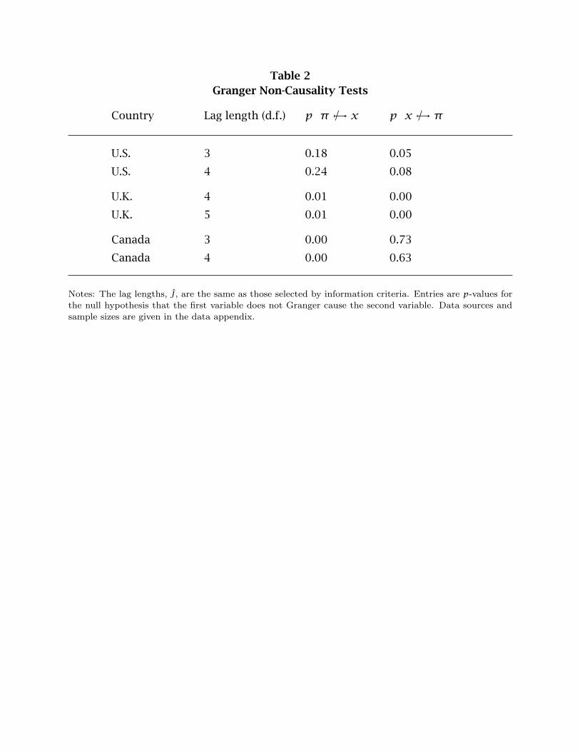
Table 2Granger Non-Causality Tests

Country Lag length (d.f.) p π �� → x p x �� → π

U.S. 3 0.18 0.05

U.S. 4 0.24 0.08

U.K. 4 0.01 0.00

U.K. 5 0.01 0.00

Canada 3 0.00 0.73

Canada 4 0.00 0.63

Notes: The lag lengths, J, are the same as those selected by information criteria. Entries are p-values forthe null hypothesis that the first variable does not Granger cause the second variable. Data sources andsample sizes are given in the data appendix.

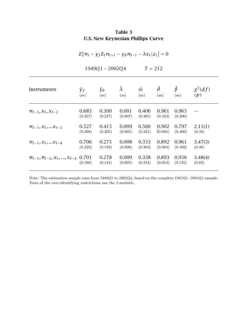
Table 3U.S. New Keynesian Phillips Curve

E[πt − γfEtπt+1 − γbπt−1 − λxt|zt

] = 0

1949Q1 – 2002Q4 T = 212

Instruments γf γb λ ω θ β χ2(df)(se) (se) (se) (se) (se) (se) (p)

πt−1, xt, xt−2 0.685 0.300 0.001 0.406 0.961 0.965 —(0.357) (0.247) (0.007) (0.465) (0.163) (0.306)

πt−1, xt, ...xt−2 0.527 0.415 0.009 0.566 0.902 0.797 2.11(1)(0.298) (0.205) (0.005) (0.321) (0.094) (0.480) (0.34)

πt−1, xt, ...xt−4 0.706 0.275 0.008 0.333 0.892 0.961 3.47(3)(0.223) (0.158) (0.006) (0.263) (0.064) (0.169) (0.48)

πt−1, πt−2, xt, ..., xt−4 0.701 0.278 0.009 0.338 0.893 0.956 3.48(4)(0.188) (0.141) (0.005) (0.234) (0.054) (0.135) (0.63)

Note: The estimation sample runs from 1949Q1 to 2002Q4, based on the complete 1947Q1−2001Q2 sample.Tests of the over-identifying restrictions use the J-statistic.

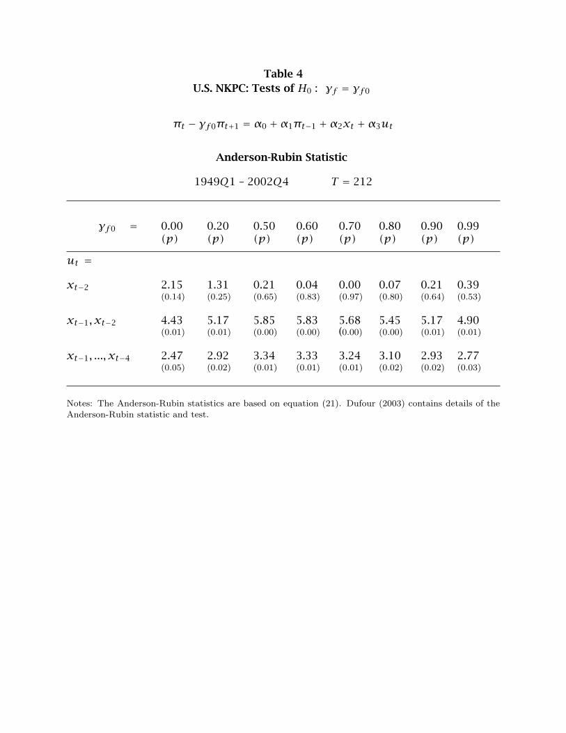
Table 4U.S. NKPC: Tests of H0 : γf = γf0

πt − γf0πt+1 = α0 +α1πt−1 +α2xt +α3ut

Anderson-Rubin Statistic

1949Q1 – 2002Q4 T = 212

γf0 = 0.00 0.20 0.50 0.60 0.70 0.80 0.90 0.99(p) (p) (p) (p) (p) (p) (p) (p)

ut =

xt−2 2.15 1.31 0.21 0.04 0.00 0.07 0.21 0.39(0.14) (0.25) (0.65) (0.83) (0.97) (0.80) (0.64) (0.53)

xt−1, xt−2 4.43 5.17 5.85 5.83 5.68 5.45 5.17 4.90(0.01) (0.01) (0.00) (0.00) (0.00) (0.00) (0.01) (0.01)

xt−1, ..., xt−4 2.47 2.92 3.34 3.33 3.24 3.10 2.93 2.77(0.05) (0.02) (0.01) (0.01) (0.01) (0.02) (0.02) (0.03)

Notes: The Anderson-Rubin statistics are based on equation (21). Dufour (2003) contains details of theAnderson-Rubin statistic and test.

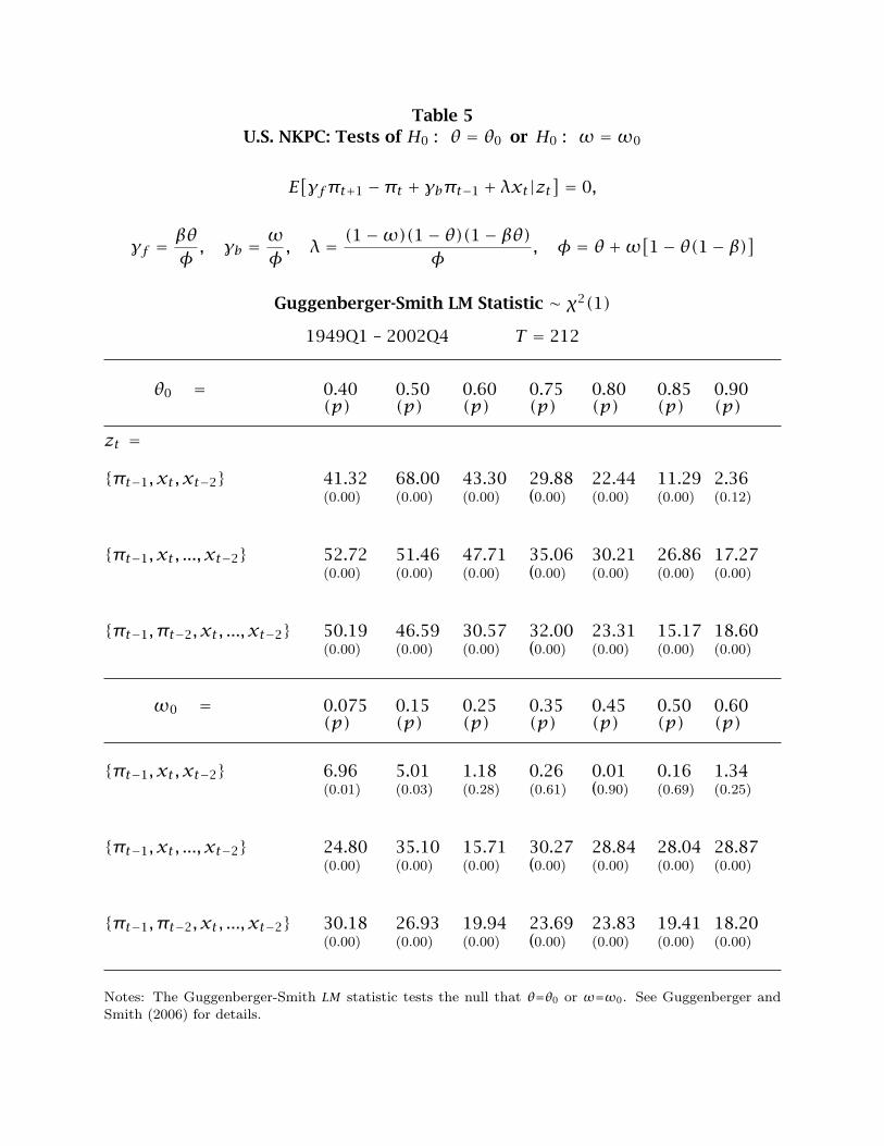
Table 5U.S. NKPC: Tests of H0 : θ = θ0 or H0 : ω =ω0

E[γfπt+1 −πt + γbπt−1 + λxt|zt

] = 0,


, φ = θ +ω[1− θ(1− β)]Guggenberger-Smith LM Statistic ∼ χ2(1)

1949Q1 – 2002Q4 T = 212

θ0 = 0.40 0.50 0.60 0.75 0.80 0.85 0.90(p) (p) (p) (p) (p) (p) (p)

zt =

{πt−1, xt, xt−2} 41.32 68.00 43.30 29.88 22.44 11.29 2.36(0.00) (0.00) (0.00) (0.00) (0.00) (0.00) (0.12)

{πt−1, xt, ..., xt−2} 52.72 51.46 47.71 35.06 30.21 26.86 17.27(0.00) (0.00) (0.00) (0.00) (0.00) (0.00) (0.00)

{πt−1, πt−2, xt, ..., xt−2} 50.19 46.59 30.57 32.00 23.31 15.17 18.60(0.00) (0.00) (0.00) (0.00) (0.00) (0.00) (0.00)

ω0 = 0.075 0.15 0.25 0.35 0.45 0.50 0.60(p) (p) (p) (p) (p) (p) (p)

{πt−1, xt, xt−2} 6.96 5.01 1.18 0.26 0.01 0.16 1.34(0.01) (0.03) (0.28) (0.61) (0.90) (0.69) (0.25)

{πt−1, xt, ..., xt−2} 24.80 35.10 15.71 30.27 28.84 28.04 28.87(0.00) (0.00) (0.00) (0.00) (0.00) (0.00) (0.00)

{πt−1, πt−2, xt, ..., xt−2} 30.18 26.93 19.94 23.69 23.83 19.41 18.20(0.00) (0.00) (0.00) (0.00) (0.00) (0.00) (0.00)

Notes: The Guggenberger-Smith LM statistic tests the null that θ=θ0 or ω=ω0. See Guggenberger andSmith (2006) for details.

Table 6U.K. New Keynesian Phillips Curve


]1961Q1 – 2000Q4 T = 168


πt−1, xt, xt−1 -2.699 2.396 0.924 0.702 0.492 -1.608 —(4.782) (3.047) (1.531) (0.113) (0.337) (1.412)

πt−1, xt−1, ..., xt−4 0.935 0.019 0.334 0.011 0.570 0.953 4.40(2)(0.266) (0.192) (0.152) (0.114) (0.065) (0.113) (0.22)

πt−1, xt, ..., xt−4 0.234 0.535 0.062 0.562 0.801 0.307 9.82(3)(0.200) (0.120) (0.133) (0.139) (0.303) (0.287) (0.04)

πt−1, πt−2, xt, ..., xt−4 0.233 0.621 -0.045 0.842 1.569 0.201 15.94(4)(0.153) (0.107) (0.089) (0.224) (2.120) (0.242) (0.01)

Notes: The estimation sample runs from 1961Q1 to 2000Q4, based on the complete 1959Q3−2001Q2 sample.Otherwise, see the notes to table 3.

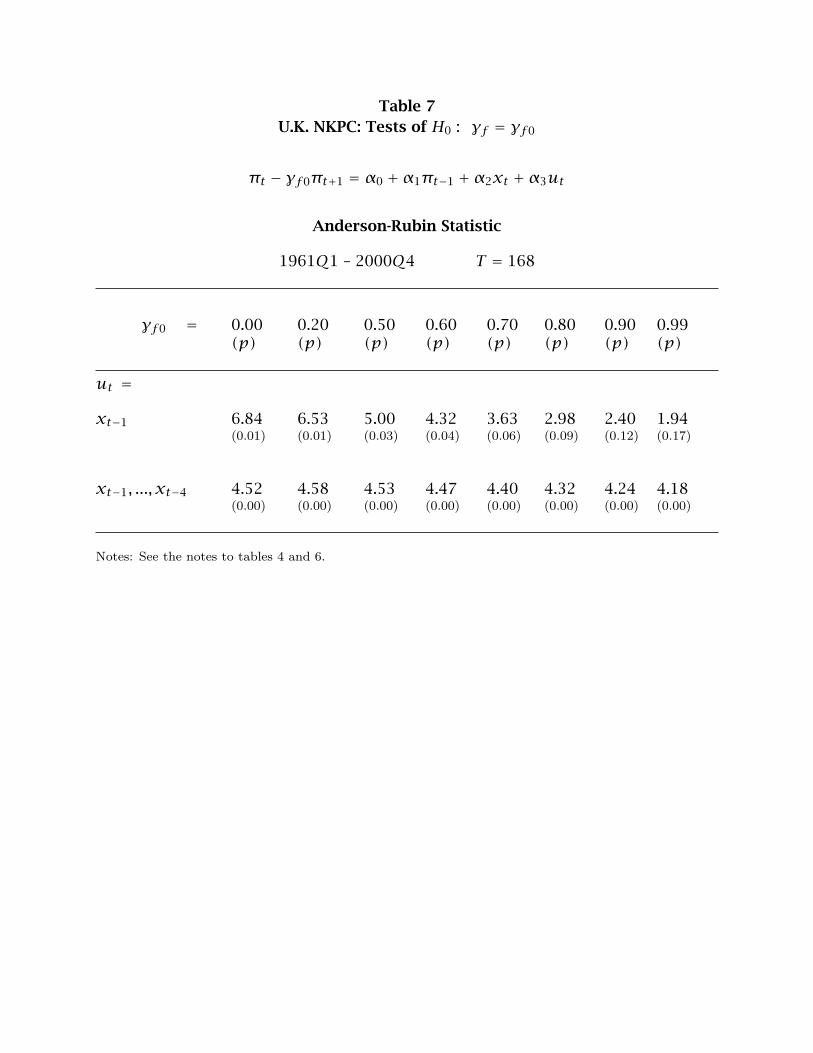
Table 7U.K. NKPC: Tests of H0 : γf = γf0



1961Q1 – 2000Q4 T = 168

γf0 = 0.00 0.20 0.50 0.60 0.70 0.80 0.90 0.99(p) (p) (p) (p) (p) (p) (p) (p)

ut =

xt−1 6.84 6.53 5.00 4.32 3.63 2.98 2.40 1.94(0.01) (0.01) (0.03) (0.04) (0.06) (0.09) (0.12) (0.17)

xt−1, ..., xt−4 4.52 4.58 4.53 4.47 4.40 4.32 4.24 4.18(0.00) (0.00) (0.00) (0.00) (0.00) (0.00) (0.00) (0.00)

Notes: See the notes to tables 4 and 6.

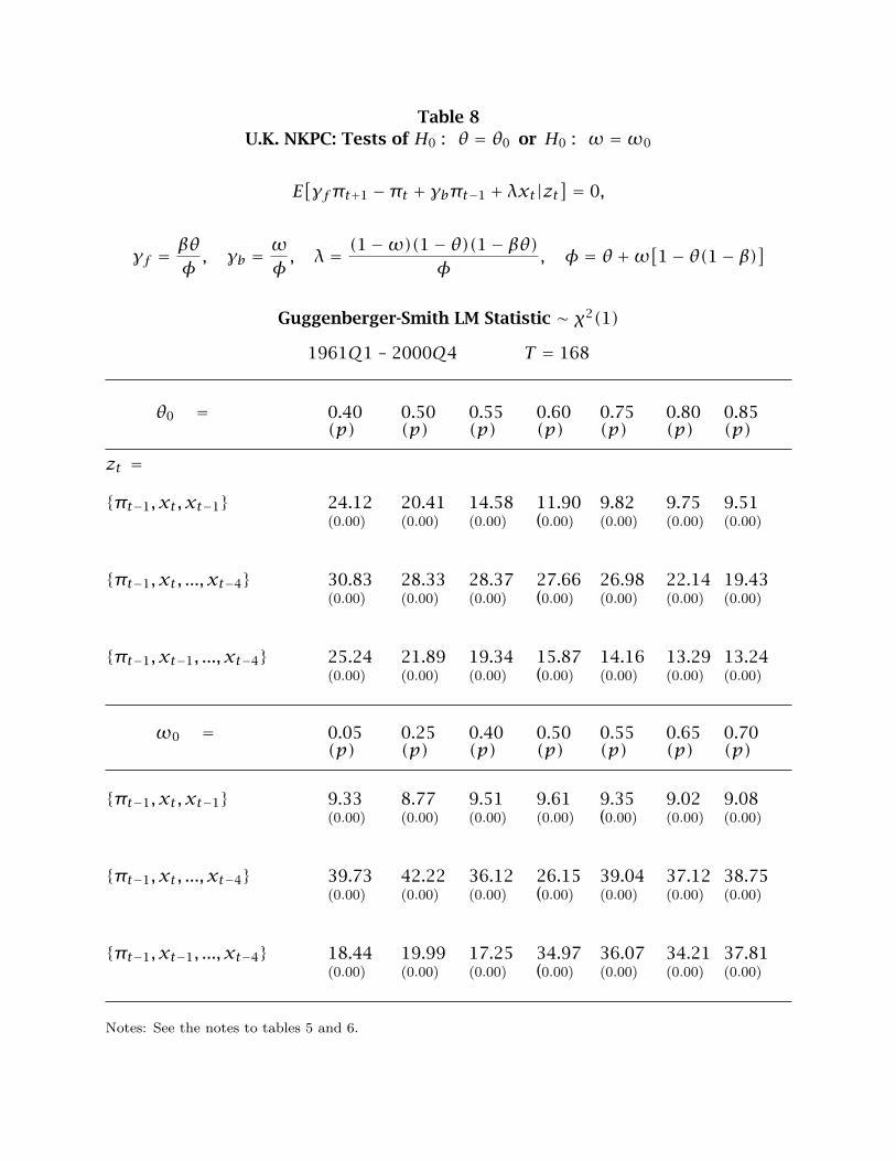
Table 8U.K. NKPC: Tests of H0 : θ = θ0 or H0 : ω =ω0


] = 0,


, φ = θ +ω[1− θ(1− β)]

Guggenberger-Smith LM Statistic ∼ χ2(1)

1961Q1 – 2000Q4 T = 168

θ0 = 0.40 0.50 0.55 0.60 0.75 0.80 0.85(p) (p) (p) (p) (p) (p) (p)

zt =

{πt−1, xt, xt−1} 24.12 20.41 14.58 11.90 9.82 9.75 9.51(0.00) (0.00) (0.00) (0.00) (0.00) (0.00) (0.00)

{πt−1, xt, ..., xt−4} 30.83 28.33 28.37 27.66 26.98 22.14 19.43(0.00) (0.00) (0.00) (0.00) (0.00) (0.00) (0.00)

{πt−1, xt−1, ..., xt−4} 25.24 21.89 19.34 15.87 14.16 13.29 13.24(0.00) (0.00) (0.00) (0.00) (0.00) (0.00) (0.00)

ω0 = 0.05 0.25 0.40 0.50 0.55 0.65 0.70(p) (p) (p) (p) (p) (p) (p)

{πt−1, xt, xt−1} 9.33 8.77 9.51 9.61 9.35 9.02 9.08(0.00) (0.00) (0.00) (0.00) (0.00) (0.00) (0.00)

{πt−1, xt, ..., xt−4} 39.73 42.22 36.12 26.15 39.04 37.12 38.75(0.00) (0.00) (0.00) (0.00) (0.00) (0.00) (0.00)

{πt−1, xt−1, ..., xt−4} 18.44 19.99 17.25 34.97 36.07 34.21 37.81(0.00) (0.00) (0.00) (0.00) (0.00) (0.00) (0.00)


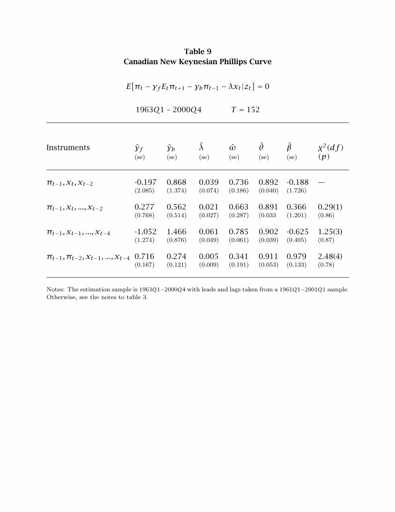
Table 9Canadian New Keynesian Phillips Curve


] = 0

1963Q1 – 2000Q4 T = 152


πt−1, xt, xt−2 -0.197 0.868 0.039 0.736 0.892 -0.188 —(2.085) (1.374) (0.074) (0.186) (0.040) (1.726)

πt−1, xt, ..., xt−2 0.277 0.562 0.021 0.663 0.891 0.366 0.29(1)(0.768) (0.514) (0.027) (0.287) (0.033 (1.201) (0.86)

πt−1, xt−1, ..., xt−4 -1.052 1.466 0.061 0.785 0.902 -0.625 1.25(3)(1.274) (0.876) (0.049) (0.061) (0.039) (0.405) (0.87)

πt−1, πt−2, xt−1, ..., xt−4 0.716 0.274 0.005 0.341 0.911 0.979 2.48(4)(0.167) (0.121) (0.009) (0.191) (0.053) (0.133) (0.78)

Notes: The estimation sample is 1963Q1−2000Q4 with leads and lags taken from a 1961Q1−2001Q1 sample.Otherwise, see the notes to table 3.

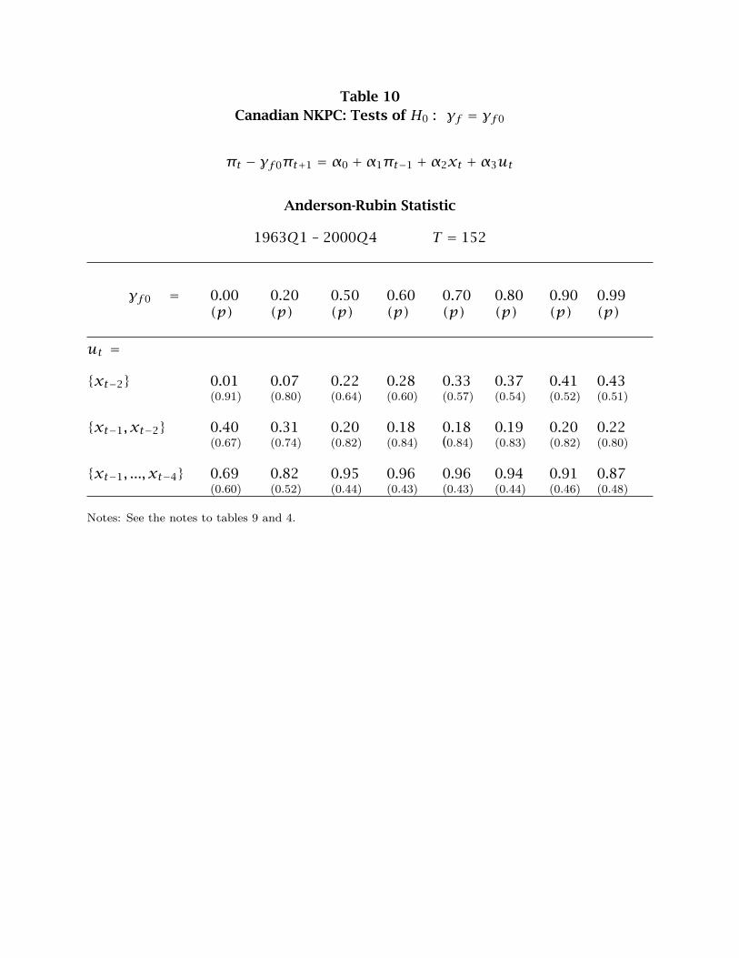
Table 10Canadian NKPC: Tests of H0 : γf = γf0



1963Q1 – 2000Q4 T = 152

γf0 = 0.00 0.20 0.50 0.60 0.70 0.80 0.90 0.99(p) (p) (p) (p) (p) (p) (p) (p)

ut =

{xt−2} 0.01 0.07 0.22 0.28 0.33 0.37 0.41 0.43(0.91) (0.80) (0.64) (0.60) (0.57) (0.54) (0.52) (0.51)

{xt−1, xt−2} 0.40 0.31 0.20 0.18 0.18 0.19 0.20 0.22(0.67) (0.74) (0.82) (0.84) (0.84) (0.83) (0.82) (0.80)

{xt−1, ..., xt−4} 0.69 0.82 0.95 0.96 0.96 0.94 0.91 0.87(0.60) (0.52) (0.44) (0.43) (0.43) (0.44) (0.46) (0.48)


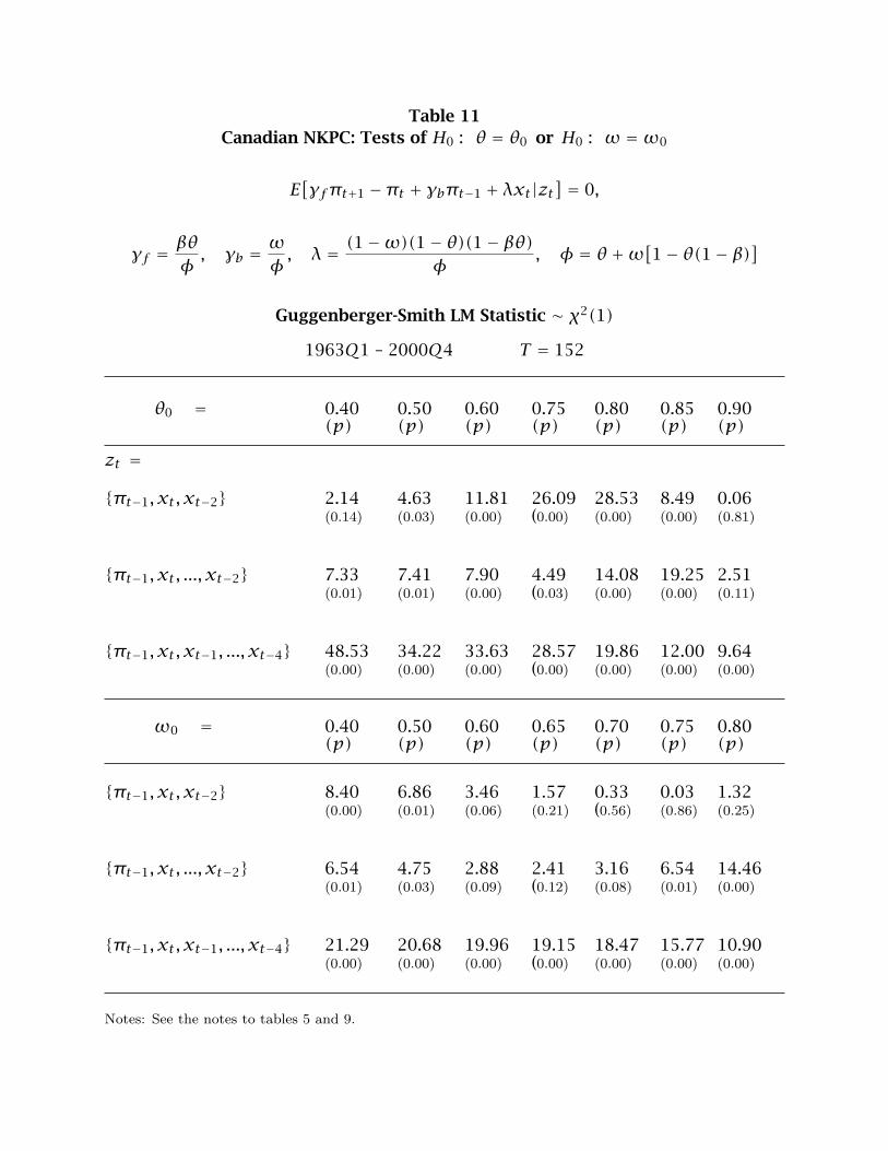
Table 11Canadian NKPC: Tests of H0 : θ = θ0 or H0 : ω =ω0


] = 0,


, φ = θ +ω[1− θ(1− β)]

Guggenberger-Smith LM Statistic ∼ χ2(1)

1963Q1 – 2000Q4 T = 152

θ0 = 0.40 0.50 0.60 0.75 0.80 0.85 0.90(p) (p) (p) (p) (p) (p) (p)

zt =

{πt−1, xt, xt−2} 2.14 4.63 11.81 26.09 28.53 8.49 0.06(0.14) (0.03) (0.00) (0.00) (0.00) (0.00) (0.81)

{πt−1, xt, ..., xt−2} 7.33 7.41 7.90 4.49 14.08 19.25 2.51(0.01) (0.01) (0.00) (0.03) (0.00) (0.00) (0.11)

{πt−1, xt, xt−1, ..., xt−4} 48.53 34.22 33.63 28.57 19.86 12.00 9.64(0.00) (0.00) (0.00) (0.00) (0.00) (0.00) (0.00)

ω0 = 0.40 0.50 0.60 0.65 0.70 0.75 0.80(p) (p) (p) (p) (p) (p) (p)

{πt−1, xt, xt−2} 8.40 6.86 3.46 1.57 0.33 0.03 1.32(0.00) (0.01) (0.06) (0.21) (0.56) (0.86) (0.25)

{πt−1, xt, ..., xt−2} 6.54 4.75 2.88 2.41 3.16 6.54 14.46(0.01) (0.03) (0.09) (0.12) (0.08) (0.01) (0.00)

{πt−1, xt, xt−1, ..., xt−4} 21.29 20.68 19.96 19.15 18.47 15.77 10.90(0.00) (0.00) (0.00) (0.00) (0.00) (0.00) (0.00)


Auxiliary Tables

Joint Tests

Not for Publication

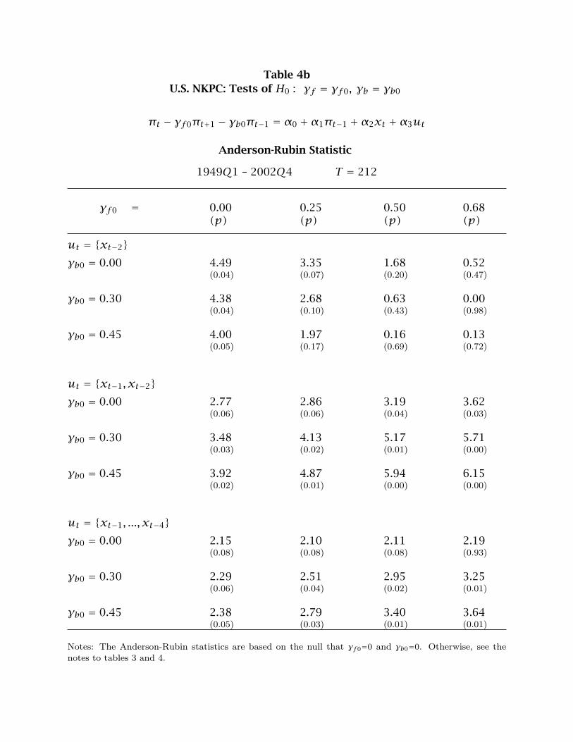
Table 4bU.S. NKPC: Tests of H0 : γf = γf0, γb = γb0

πt − γf0πt+1 − γb0πt−1 = α0 +α1πt−1 +α2xt +α3ut


1949Q1 – 2002Q4 T = 212

γf0 = 0.00 0.25 0.50 0.68(p) (p) (p) (p)

ut = {xt−2}γb0 = 0.00 4.49 3.35 1.68 0.52

(0.04) (0.07) (0.20) (0.47)

γb0 = 0.30 4.38 2.68 0.63 0.00(0.04) (0.10) (0.43) (0.98)

γb0 = 0.45 4.00 1.97 0.16 0.13(0.05) (0.17) (0.69) (0.72)

ut = {xt−1, xt−2}γb0 = 0.00 2.77 2.86 3.19 3.62

(0.06) (0.06) (0.04) (0.03)

γb0 = 0.30 3.48 4.13 5.17 5.71(0.03) (0.02) (0.01) (0.00)

γb0 = 0.45 3.92 4.87 5.94 6.15(0.02) (0.01) (0.00) (0.00)

ut = {xt−1, ..., xt−4}γb0 = 0.00 2.15 2.10 2.11 2.19

(0.08) (0.08) (0.08) (0.93)

γb0 = 0.30 2.29 2.51 2.95 3.25(0.06) (0.04) (0.02) (0.01)

γb0 = 0.45 2.38 2.79 3.40 3.64(0.05) (0.03) (0.01) (0.01)

Notes: The Anderson-Rubin statistics are based on the null that γf0=0 and γb0=0. Otherwise, see thenotes to tables 3 and 4.

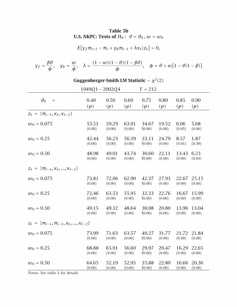
Table 5bU.S. NKPC: Tests of H0 : θ = θ0 , ω =ω0


] = 0,



1949Q1 – 2002Q4 T = 212

θ0 = 0.40 0.50 0.60 0.75 0.80 0.85 0.90(p) (p) (p) (p) (p) (p) (p)

zt = {πt−1, xt, xt−2}

ω0 = 0.075 53.51 39.29 63.91 34.67 19.52 6.06 5.68(0.00) (0.00) (0.00) (0.00) (0.00) (0.05) (0.06)

ω0 = 0.25 42.44 56.23 56.39 33.11 24.79 8.57 1.87(0.00) (0.00) (0.00) (0.00) (0.00) (0.01) (0.39)

ω0 = 0.50 48.98 49.01 43.74 30.60 22.11 13.43 6.23(0.00) (0.00) (0.00) (0.00) (0.00) (0.00) (0.04)

zt = {πt−1, xt, ..., xt−2}

ω0 = 0.075 73.81 72.06 62.90 42.37 27.93 22.67 25.15(0.00) (0.00) (0.00) (0.00) (0.00) (0.00) (0.00)

ω0 = 0.25 72.46 63.53 55.95 32.33 22.76 16.67 15.99(0.00) (0.00) (0.00) (0.00) (0.00) (0.00) (0.00)

ω0 = 0.50 49.15 49.32 48.64 30.08 20.80 13.96 13.04(0.00) (0.00) (0.00) (0.00) (0.00) (0.00) (0.00)

zt = {πt−1, πt−2, xt, ..., xt−2}

ω0 = 0.075 73.99 71.63 63.57 40.27 31.77 21.72 21.84(0.00) (0.00) (0.00) (0.00) (0.00) (0.00) (0.00)

ω0 = 0.25 68.88 65.91 56.60 29.97 20.47 16.29 22.65(0.00) (0.00) (0.00) (0.00) (0.00) (0.00) (0.00)

ω0 = 0.50 64.65 52.19 52.95 35.88 22.80 16.66 20.36(0.00) (0.00) (0.00) (0.00) (0.00) (0.00) (0.00)

Notes: See table 5 for details.

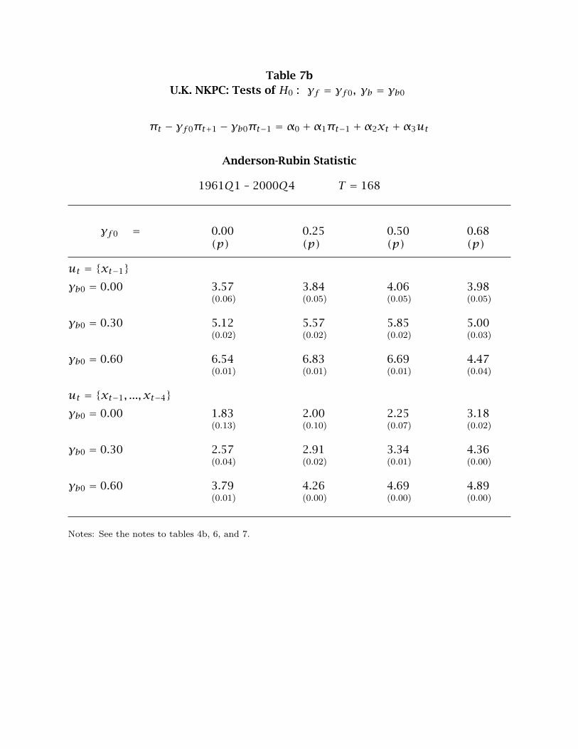
Table 7bU.K. NKPC: Tests of H0 : γf = γf0, γb = γb0



1961Q1 – 2000Q4 T = 168

γf0 = 0.00 0.25 0.50 0.68(p) (p) (p) (p)

ut = {xt−1}γb0 = 0.00 3.57 3.84 4.06 3.98

(0.06) (0.05) (0.05) (0.05)

γb0 = 0.30 5.12 5.57 5.85 5.00(0.02) (0.02) (0.02) (0.03)

γb0 = 0.60 6.54 6.83 6.69 4.47(0.01) (0.01) (0.01) (0.04)

ut = {xt−1, ..., xt−4}γb0 = 0.00 1.83 2.00 2.25 3.18

(0.13) (0.10) (0.07) (0.02)

γb0 = 0.30 2.57 2.91 3.34 4.36(0.04) (0.02) (0.01) (0.00)

γb0 = 0.60 3.79 4.26 4.69 4.89(0.01) (0.00) (0.00) (0.00)

Notes: See the notes to tables 4b, 6, and 7.

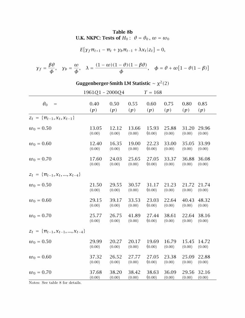
Table 8bU.K. NKPC: Tests of H0 : θ = θ0 , ω =ω0


] = 0,



1961Q1 – 2000Q4 T = 168

θ0 = 0.40 0.50 0.55 0.60 0.75 0.80 0.85(p) (p) (p) (p) (p) (p) (p)

zt = {πt−1, xt, xt−1}

ω0 = 0.50 13.05 12.12 13.66 15.93 25.88 31.20 29.96(0.00) (0.00) (0.00) (0.00) (0.00) (0.00) (0.00)

ω0 = 0.60 12.40 16.35 19.00 22.23 33.00 35.05 33.99(0.00) (0.00) (0.00) (0.00) (0.00) (0.00) (0.00)

ω0 = 0.70 17.60 24.03 25.65 27.05 33.37 36.88 36.08(0.00) (0.00) (0.00) (0.00) (0.00) (0.00) (0.00)

zt = {πt−1, xt, ..., xt−4}

ω0 = 0.50 21.50 29.55 30.57 31.17 21.23 21.72 21.74(0.00) (0.00) (0.00) (0.00) (0.00) (0.00) (0.00)

ω0 = 0.60 29.15 39.17 33.53 23.03 22.64 40.43 48.32(0.00) (0.00) (0.00) (0.00) (0.00) (0.00) (0.00)

ω0 = 0.70 25.77 26.75 41.89 27.44 38.61 22.64 38.16(0.00) (0.00) (0.00) (0.00) (0.00) (0.00) (0.00)

zt = {πt−1, xt−1, ..., xt−4}

ω0 = 0.50 29.99 20.27 20.17 19.69 16.79 15.45 14.72(0.00) (0.00) (0.00) (0.00) (0.00) (0.00) (0.00)

ω0 = 0.60 37.32 26.52 27.77 27.05 23.38 25.09 22.88(0.00) (0.00) (0.00) (0.00) (0.00) (0.00) (0.00)

ω0 = 0.70 37.68 38.20 38.42 38.63 36.09 29.56 32.16(0.00) (0.00) (0.00) (0.00) (0.00) (0.00) (0.00)


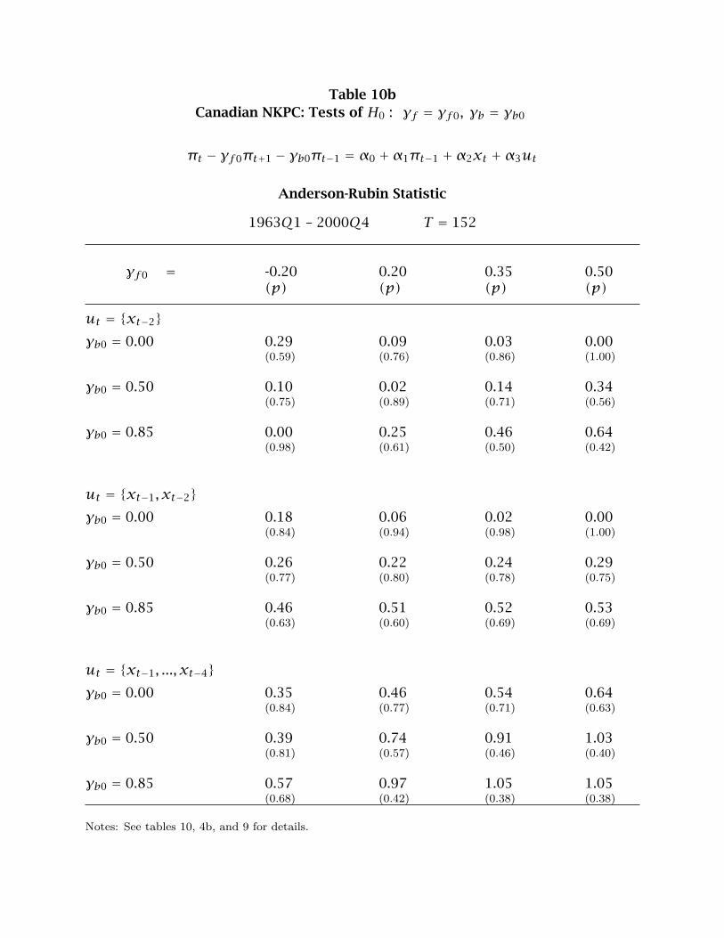
Table 10bCanadian NKPC: Tests of H0 : γf = γf0, γb = γb0



1963Q1 – 2000Q4 T = 152

γf0 = -0.20 0.20 0.35 0.50(p) (p) (p) (p)

ut = {xt−2}γb0 = 0.00 0.29 0.09 0.03 0.00

(0.59) (0.76) (0.86) (1.00)

γb0 = 0.50 0.10 0.02 0.14 0.34(0.75) (0.89) (0.71) (0.56)

γb0 = 0.85 0.00 0.25 0.46 0.64(0.98) (0.61) (0.50) (0.42)

ut = {xt−1, xt−2}γb0 = 0.00 0.18 0.06 0.02 0.00

(0.84) (0.94) (0.98) (1.00)

γb0 = 0.50 0.26 0.22 0.24 0.29(0.77) (0.80) (0.78) (0.75)

γb0 = 0.85 0.46 0.51 0.52 0.53(0.63) (0.60) (0.69) (0.69)

ut = {xt−1, ..., xt−4}γb0 = 0.00 0.35 0.46 0.54 0.64

(0.84) (0.77) (0.71) (0.63)

γb0 = 0.50 0.39 0.74 0.91 1.03(0.81) (0.57) (0.46) (0.40)

γb0 = 0.85 0.57 0.97 1.05 1.05(0.68) (0.42) (0.38) (0.38)

Notes: See tables 10, 4b, and 9 for details.

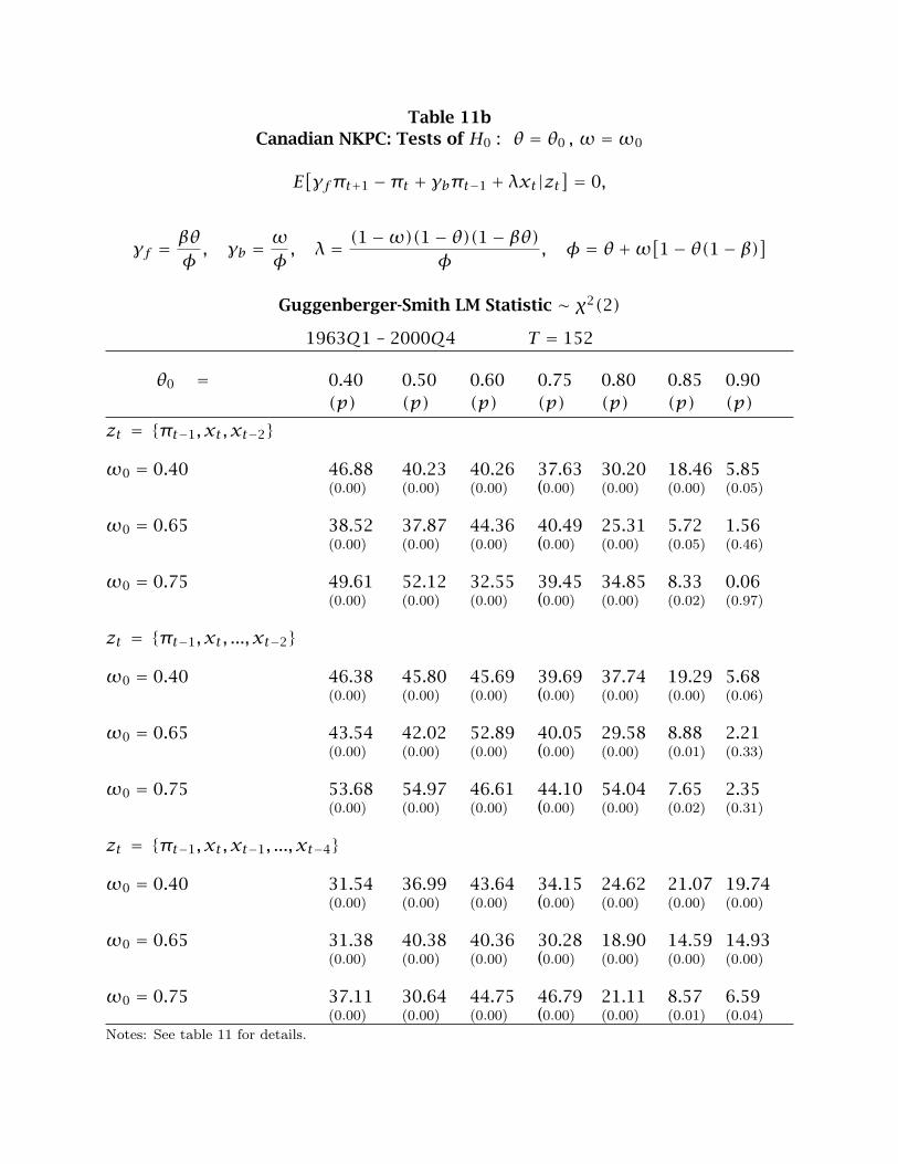
Table 11bCanadian NKPC: Tests of H0 : θ = θ0 , ω =ω0


] = 0,



1963Q1 – 2000Q4 T = 152

θ0 = 0.40 0.50 0.60 0.75 0.80 0.85 0.90(p) (p) (p) (p) (p) (p) (p)

zt = {πt−1, xt, xt−2}

ω0 = 0.40 46.88 40.23 40.26 37.63 30.20 18.46 5.85(0.00) (0.00) (0.00) (0.00) (0.00) (0.00) (0.05)

ω0 = 0.65 38.52 37.87 44.36 40.49 25.31 5.72 1.56(0.00) (0.00) (0.00) (0.00) (0.00) (0.05) (0.46)

ω0 = 0.75 49.61 52.12 32.55 39.45 34.85 8.33 0.06(0.00) (0.00) (0.00) (0.00) (0.00) (0.02) (0.97)

zt = {πt−1, xt, ..., xt−2}

ω0 = 0.40 46.38 45.80 45.69 39.69 37.74 19.29 5.68(0.00) (0.00) (0.00) (0.00) (0.00) (0.00) (0.06)

ω0 = 0.65 43.54 42.02 52.89 40.05 29.58 8.88 2.21(0.00) (0.00) (0.00) (0.00) (0.00) (0.01) (0.33)

ω0 = 0.75 53.68 54.97 46.61 44.10 54.04 7.65 2.35(0.00) (0.00) (0.00) (0.00) (0.00) (0.02) (0.31)

zt = {πt−1, xt, xt−1, ..., xt−4}

ω0 = 0.40 31.54 36.99 43.64 34.15 24.62 21.07 19.74(0.00) (0.00) (0.00) (0.00) (0.00) (0.00) (0.00)

ω0 = 0.65 31.38 40.38 40.36 30.28 18.90 14.59 14.93(0.00) (0.00) (0.00) (0.00) (0.00) (0.00) (0.00)

ω0 = 0.75 37.11 30.64 44.75 46.79 21.11 8.57 6.59(0.00) (0.00) (0.00) (0.00) (0.00) (0.01) (0.04)


Identifying the New Keynesian Phillips...

Documents

Transcript of Identifying the New Keynesian Phillips...