The method of fundamental solutions for the Cauchy problem in two-dimensional linear elasticity
14
The method of fundamental solutions for the Cauchy problem in two-dimensional linear elasticity Liviu Marin a, * , Daniel Lesnic b a School of the Environment, University of Leeds, Leeds LS2 9JT, UK b Department of Applied Mathematics, University of Leeds, Leeds LS2 9JT, UK Received 20 January 2004; received in revised form 20 January 2004 Available online 11 March 2004 Abstract In this paper, the application of the method of fundamental solutions to the Cauchy problem in two-dimensional isotropic linear elasticity is investigated. The resulting system of linear algebraic equations is ill-conditioned and therefore its solution is regularised by employing the first-order Tikhonov functional, while the choice of the regu- larisation parameter is based on the L-curve method. Numerical results are presented for both smooth and piecewise smooth geometries, as well as for constant and linear stress states. The convergence and the stability of the method with respect to increasing the number of source points and the distance between the source points and the boundary of the solution domain, and decreasing the amount of noise added into the input data, respectively, are analysed. Ó 2004 Elsevier Ltd. All rights reserved. Keywords: Meshless method; Method of fundamental solutions; Cauchy problem; Linear elasticity; Regularisation; Inverse problem 1. Introduction The method of fundamental solutions (MFS) was originally introduced by Kupradze and Aleksidze (1964), whilst its numerical formulation was first given by Mathon and Johnston (1977). The main idea of the MFS consists of approximating the solution of the problem by a linear combination of fundamental solutions with respect to some singularities/source points which are located outside the domain. Then, the original problem is reduced to determining the unknown coefficients of the fundamental solutions and the coordinates of the source points by requiring the approximation to satisfy the boundary conditions and hence solving a non-linear problem. If the source points are a priori fixed then the coefficients of the MFS approximation are determined by solving a linear problem. An excellent survey of the MFS and related methods over the past three decades has been presented by Fairweather and Karageorghis (1998). The advantages of the MFS over domain discretisation methods, such as the finite difference (FDM) and the finite element methods (FEM), are very well documented (see e.g. Fairweather and Karageorghis, * Corresponding author. Tel.: +44-0113-3436744; fax: +44-0113-3436716. E-mail address: [email protected] (L. Marin). 0020-7683/$ - see front matter Ó 2004 Elsevier Ltd. All rights reserved. doi:10.1016/j.ijsolstr.2004.02.009 International Journal of Solids and Structures 41 (2004) 3425–3438 www.elsevier.com/locate/ijsolstr
-
Upload
liviu-marin -
Category
Documents
-
view
215 -
download
3
Transcript of The method of fundamental solutions for the Cauchy problem in two-dimensional linear elasticity

International Journal of Solids and Structures 41 (2004) 3425–3438
www.elsevier.com/locate/ijsolstr
The method of fundamental solutions for the Cauchyproblem in two-dimensional linear elasticity
Liviu Marin a,*, Daniel Lesnic b
a School of the Environment, University of Leeds, Leeds LS2 9JT, UKb Department of Applied Mathematics, University of Leeds, Leeds LS2 9JT, UK
Received 20 January 2004; received in revised form 20 January 2004
Available online 11 March 2004
Abstract
In this paper, the application of the method of fundamental solutions to the Cauchy problem in two-dimensional
isotropic linear elasticity is investigated. The resulting system of linear algebraic equations is ill-conditioned and
therefore its solution is regularised by employing the first-order Tikhonov functional, while the choice of the regu-
larisation parameter is based on the L-curve method. Numerical results are presented for both smooth and piecewise
smooth geometries, as well as for constant and linear stress states. The convergence and the stability of the method with
respect to increasing the number of source points and the distance between the source points and the boundary of the
solution domain, and decreasing the amount of noise added into the input data, respectively, are analysed.
� 2004 Elsevier Ltd. All rights reserved.
Keywords: Meshless method; Method of fundamental solutions; Cauchy problem; Linear elasticity; Regularisation; Inverse problem
1. Introduction
The method of fundamental solutions (MFS) was originally introduced by Kupradze and Aleksidze
(1964), whilst its numerical formulation was first given by Mathon and Johnston (1977). The main idea of
the MFS consists of approximating the solution of the problem by a linear combination of fundamental
solutions with respect to some singularities/source points which are located outside the domain. Then, theoriginal problem is reduced to determining the unknown coefficients of the fundamental solutions and the
coordinates of the source points by requiring the approximation to satisfy the boundary conditions and
hence solving a non-linear problem. If the source points are a priori fixed then the coefficients of the MFS
approximation are determined by solving a linear problem. An excellent survey of the MFS and related
methods over the past three decades has been presented by Fairweather and Karageorghis (1998).
The advantages of the MFS over domain discretisation methods, such as the finite difference (FDM) and
the finite element methods (FEM), are very well documented (see e.g. Fairweather and Karageorghis,
* Corresponding author. Tel.: +44-0113-3436744; fax: +44-0113-3436716.
E-mail address: [email protected] (L. Marin).
0020-7683/$ - see front matter � 2004 Elsevier Ltd. All rights reserved.
doi:10.1016/j.ijsolstr.2004.02.009

3426 L. Marin, D. Lesnic / International Journal of Solids and Structures 41 (2004) 3425–3438
1998). In addition, the MFS has all the advantages of boundary methods, such as the boundary element
method (BEM), as well as several advantages over other boundary methods. For example, the MFS does
not require an elaborate discretisation of the boundary, integrations over the boundary are avoided, the
solution in the interior of the domain is evaluated without extra quadratures, its implementation is veryeasy and only little data preparation is required. The most arguable issue regarding the MFS is still the
location of the source points. However, this problem can be overcome by employing a non-linear least-
squares minimisation procedure. Alternatively, the source points can be prescribed a priori (see Bala-
krishnan and Ramachandran, 1999; Golberg and Chen, 1996, 1999) and the post-processing analysis of the
errors can indicate their optimal location.
The MFS has been successfully applied for solving a wide variety of boundary value problems. Kara-
georghis and Fairweather (1987) have solved numerically the biharmonic equation using the MFS and later
their method has been modified in order to take into account the presence of boundary singularities in boththe Laplace and the biharmonic equations by Poullikkas et al. (1998a). Furthermore, Poullikkas et al.
(1998b) have investigated the numerical solutions of the inhomogeneous harmonic and biharmonic
equations by reducing these problems to the homogeneous corresponding cases and subtracting a particular
solution of the governing equation. The MFS has been formulated for three-dimensional Signorini
boundary value problems and it has been tested on a three-dimensional electropainting problem related to
the coating of vehicle roofs in Poullikkas et al. (2001). Whilst Karageorghis and Fairweather (2000) have
studied the use of the MFS for the approximate solution of three-dimensional isotropic materials with
axisymmetrical geometry and both axisymmetrical and arbitrary boundary conditions. The application ofthe MFS to two-dimensional problems of steady-state heat conduction and elastostatics in isotropic and
anisotropic bimaterials has been addressed by Berger and Karageorghis (1999, 2001). Karageorghis (2001)
has investigated the calculation of the eigenvalues of the Helmholtz equation subject to homogeneous
Dirichlet boundary conditions for circular and rectangular geometries by employing the MFS, whilst
Poullikkas et al. (2002) have successfully applied the MFS for solving three-dimensional elastostatics
problems. The MFS, in conjunction with singular value decomposition, has been employed by Rama-
chandran (2002) in order to obtain numerical solutions of the Laplace and the Helmholtz equations. Re-
cently, Balakrishnan et al. (2002) have proposed an operator splitting-radial basis function method as ageneric solution procedure for transient nonlinear Poisson problems by combining the concepts of operator
splitting, radial basis function interpolation, particular solutions and the MFS.
In most boundary value problems in solid mechanics, the governing system of partial differential
equations, i.e. the equilibrium, constitutive and kinematics equations, have to be solved with the appro-
priate initial and boundary conditions for the displacement and/or traction vectors, i.e. Dirichlet, Neumann
or mixed boundary conditions. These problems are called direct problems and their existence and
uniqueness have been well established (see for example Knops and Payne, 1986). However, there are other
engineering problems which do not belong to this category. For example, the material properties and/or theexternal sources are unknown, the geometry of a portion of the boundary is not determined or the
boundary conditions are incomplete, either in the form of underspecified and overspecified boundary
conditions on different parts of the boundary or the solution is prescribed at some internal points in the
domain. These are inverse problems, and it is well known that they are generally ill-posed, i.e. the existence,
uniqueness and stability of their solutions are not always guaranteed (see e.g. Hadamard, 1923).
A classical example of an inverse problem in elasticity is the Cauchy problem in which both displacement
and traction boundary conditions are prescribed only on a part of the boundary of the solution domain,
whilst no information is available on the remaining part of the boundary. This problem has been studied byYeih et al. (1993), who have analysed its existence, uniqueness and continuous dependence on the data and
have proposed an alternative regularisation procedure, namely the fictitious boundary indirect method,
based on the simple or double layer potential theory. The numerical implementation of the aforementioned
method has been undertaken by Koya et al. (1993), who have used the BEM and the Nystr€om method for
L. Marin, D. Lesnic / International Journal of Solids and Structures 41 (2004) 3425–3438 3427
discretising the integrals. However, this formulation has not yet removed the problem of multiple inte-
grations. Marin et al. (2001) have determined the approximate solutions to the Cauchy problem in linear
elasticity using an alternating iterative BEM which reduced the problem to solving a sequence of well-posed
boundary value problems and they have later extended this numerical method to singular Cauchy problems(see Marin et al., 2002a). Whilst Huang and Shih (1997) and Marin et al. (2002b) have both used the
conjugate gradient method combined with the BEM, in order to solve the same problem. Recently, the
Tikhonov regularisation method and the singular value decomposition, in conjunction with the BEM, have
been employed by Marin and Lesnic (2002a,b) to solve the two-dimensional Cauchy problem in linear
elasticity.
To our knowledge, the application of the MFS to the Cauchy problem in linear elasticity has not been
investigated yet. The MFS discretised system of equations is ill-conditioned and hence it is solved by
employing the first-order Tikhonov regularisation method (see e.g. Tikhonov and Arsenin, 1986), whilst thechoice of the regularisation parameter is based on the L-curve criterion (see Hansen, 2001). Three
benchmark examples for the two-dimensional isotropic linear elasticity involving smooth and piecewise
smooth geometries and dealing with constant and linear stress states, i.e. linear and quadratic displace-
ments, respectively, are investigated and the convergence and stability of the method with respect to the
location and the number of source points and the amount of noise added into the Cauchy input data,
respectively, are analysed.
2. Mathematical formulation
Consider an isotropic linear elastic material which occupies an open bounded domain X � R2 and as-
sume that X is bounded by a piecewise smooth curve C ¼ oX, such that C ¼ C1 [ C2, where C1;C2 6¼ ; and
C1 \ C2 ¼ ;. In the absence of body forces, the equilibrium equations with respect to the displacement
vector uðxÞ, also known as the Lam�e or Navier equations, are given by (see e.g. Landau and Lifshits, 1986)
Go2uiðxÞoxjoxj
þ G1 2m
o2ujðxÞoxioxj
¼ 0; x 2 X; i ¼ 1; 2; ð1Þ
where G and m are the shear modulus and Poisson ratio, respectively, and the customary standard Cartesiannotation for summation over repeated indices is used. The strains eijðxÞ, i; j ¼ 1, 2, are related to the dis-
placement gradients by the kinematic relations
eijðxÞ ¼1
2
ouiðxÞoxj
�þ oujðxÞ
oxi
�; x 2 X; i; j ¼ 1; 2; ð2Þ
while the stresses rijðxÞ, i; j ¼ 1; 2, are related to the strains through the constitutive law (Hooke’s law),
namely
rijðxÞ ¼ 2G eijðxÞ�
þ m1 2m
ekkðxÞ�; x 2 X; i; j ¼ 1; 2; ð3Þ
with dij the Kronecker delta tensor. We now let nðxÞ be the outward normal vector at C and tðxÞ be the
traction vector at a point x 2 C whose components are defined by
tiðxÞ ¼ rijðxÞnjðxÞ; x 2 C; i ¼ 1; 2: ð4Þ
In the direct problem formulation, the knowledge of the displacement and/or traction vectors on the whole
boundary C gives the corresponding Dirichlet, Neumann, or mixed boundary conditions which enables usto determine the displacement vector in the domain X. Then, the strain tensor eij can be calculated from the
kinematic relations (2) and the stress tensor is determined using the constitutive law (3).

3428 L. Marin, D. Lesnic / International Journal of Solids and Structures 41 (2004) 3425–3438
If it is possible to measure both the displacement and traction vectors on a part of the boundary C, say
C1, then this leads to the mathematical formulation of an inverse problem consisting of Eq. (1) and the
boundary conditions
uiðxÞ ¼ ~uiðxÞ; tiðxÞ ¼ ~tiðxÞ; x 2 C1; i ¼ 1; 2; ð5Þ
where eu and et are prescribed vector valued functions. In the above formulation of the boundary conditions(5), it can be seen that the boundary C1 is overspecified by prescribing both the displacement ujC1
¼ eu and
the traction tjC1¼ et vectors, whilst the boundary C2 is underspecified since both the displacement ujC2
and
the traction tjC2vectors are unknown and have to be determined. This problem, termed the Cauchy
problem, is much more difficult to solve both analytically and numerically than the direct problem, since the
solution does not satisfy the general conditions of well-posedness. Although the problem may have a
unique solution, it is well known (see e.g. Hadamard, 1923) that this solution is unstable with respect to
small perturbations in the data on C1. Thus the problem is ill-posed and we cannot use a direct approach,
such as the Gauss elimination method, in order to solve the system of linear equations which arises from thediscretisation of the partial differential equation (1) and the boundary conditions (5). Therefore, regular-
isation methods are required in order to solve accurately the Cauchy problem in linear elasticity.
3. Method of fundamental solutions
The fundamental solutions U ðjÞ, j ¼ 1; 2, of the Lam�e system (1) in the two-dimensional case are given by
(see e.g. Berger and Karageorghis, 2001)
U ðjÞðx; yÞ ¼ Uijðx; yÞei; x 2 X; y 2 R2 n X; j ¼ 1; 2; ð6Þ
where y is a source point, ei, i ¼ 1; 2, is the unit vector along the xi-axis and
Uijðx; yÞ ¼ 1
8pGð1 mÞ ð3�
4mÞ ln rðx; yÞdij ðxi yiÞðxj yjÞ
r2ðx; yÞ
�; i; j ¼ 1; 2: ð7Þ
Here m ¼ m for the plane strain state and m ¼ m=ð1þ mÞ in the plane stress state, rðx; yÞ ¼ffiffiffiffiffiffiffiffiffiffiffiffiffiffiffiffiffiffiffiffiffiffiffiffiffiffiffiffiffiffiffiffiffiffiffiffiffiffiffiffiffiffiffiffiðx1 y1Þ2 þ ðx2 y2Þ2
qrepresents the distance between the domain point x and the source point y and dij is
the Kronecker delta tensor.
The main idea of the MFS consists of the approximation of the displacement vector in the solu-
tion domain by a linear combination of fundamental solutions with respect to M source points yj in the
form
uðxÞ � uMða; b;Y ; xÞ ¼ ajUð1Þðx; yjÞ þ bjU
ð2Þðx; yjÞ; x 2 X; ð8Þ
where a ¼ ða1; . . . ; aMÞ, b ¼ ðb1; . . . ; bMÞ and y is a 2M-vector containing the coordinates of the source
points yj, j ¼ 1; . . . ;M . On taking into account the kinematic relations (2), the constitutive law (3), the
definitions of the components of the traction vector (4) and the fundamental solutions (6) then the traction
vector can be approximated on the boundary C by
tðxÞ � tMða; b;Y ; xÞ ¼ ajTð1Þðx; yjÞ þ bjT
ð2Þðx; yjÞ; x 2 C; ð9Þ
where
TðjÞðx; yÞ ¼ Tijðx; yÞei; x 2 C; y 2 R2 n X; j ¼ 1; 2 ð10Þ

L. Marin, D. Lesnic / International Journal of Solids and Structures 41 (2004) 3425–3438 3429
and
T1jðx; yÞ ¼ 2G1 m1 2m
oU1jðx; yÞox1
�þ m
1 2moU2jðx; yÞ
ox2
�n1ðxÞ
þ GoU1jðx; yÞ
ox2
�þ oU2jðx; yÞ
ox1
�n2ðxÞ; j ¼ 1; 2;
T2jðx; yÞ ¼ GoU1jðx; yÞ
ox2
�þ oU2jðx; yÞ
ox1
�n1ðxÞ
þ 2Gm
1 2moU1jðx; yÞ
ox1
�þ 1 m
1 2moU2jðx; yÞ
ox2
�n2ðxÞ; j ¼ 1; 2:
ð11Þ
If N collocation points xi, i ¼ 1; . . . ;N , are chosen on the overspecified boundary C1 of the solution domain
X and the location of the source points yj, j ¼ 1; . . . ;M , is set then Eqs. (8) and (9) recast as a system of 4Nlinear algebraic equations with 2M unknowns which can be generically written as
AX ¼ F; ð12Þ
where the MFS matrix A, the unknown vector X and the right-hand side vector F are given byAðk1ÞNþi;ðl1ÞMþj ¼ Uklðxi; yjÞ; Aðkþ1ÞNþi;ðl1ÞMþj ¼ Tklðxi; yjÞ;Xj ¼ aj; XMþj ¼ bj; Fðk1ÞNþi ¼ ukðxiÞ; Fðkþ1ÞNþi ¼ tkðxiÞ;i ¼ 1; . . . ;N ; j ¼ 1; . . . ;M ; k; l ¼ 1; 2:
ð13Þ
It should be noted that in order to uniquely determine the solution X of the system of linear algebraic
equations (12), i.e. the coefficients aj and bj, j ¼ 1; . . . ;M , in the approximations (8) and (9), the number Nof boundary collocation points and the number M of source points must satisfy the inequality M 6 2N .However, the system of linear algebraic equation (12) cannot be solved by direct methods, such as the least-
squares method, since such an approach would produce a highly unstable solution. Most of the standard
numerical methods cannot achieve a good accuracy in the solution of the system of linear algebraic
equation (12) due to the large value of the condition number of the matrix A which increases dramatically
as the number of boundary collocation points and source points increases. It should be mentioned that for
inverse problems, the resulting systems of linear algebraic equations are ill-conditioned, even if other well-
known numerical methods (FDM, FEM or BEM) are employed. Although the MFS system of linear
algebraic equation (12) is ill-conditioned even when dealing with direct problems, the MFS has no longerthis disadvantage in comparison with other numerical methods and, in addition, it preserves its advantages,
such as the lack of any mesh, the high accuracy of the numerical results, etc.
3.1. Tikhonov regularisation method
Several regularisation procedures have been developed to solve such ill-conditioned problems (see for
example Hansen, 1998). However, we only consider the Tikhonov regularisation method (see Tikhonov and
Arsenin, 1986) in our study since it is simple, non-iterative and it provides an explicit solution, see Eq. (16)below. Furthermore, the Tikhonov regularisation method is feasible to apply for large systems of equations
unlike the singular value decomposition which may become prohibitive for such large problems (see
Hansen, 2001).
The Tikhonov regularised solution to the system of linear algebraic equation (12) is sought as
Xk : TkðXkÞ ¼ minX2R2M
TkðXÞ; ð14Þ

3430 L. Marin, D. Lesnic / International Journal of Solids and Structures 41 (2004) 3425–3438
where Tk represents the kth order Tikhonov functional given by
Tkð�Þ : R2M ! ½0;1Þ; TkðXÞ ¼ jjAX Fjj22 þ k2jjRðkÞX jj22; ð15Þ
the matrix RðkÞ 2 Rð2MkÞ�2M induces a Ck-constraint on the solution X and k > 0 is the regularisationparameter to be chosen. Formally, the Tikhonov regularised solution Xk of the problem (14) is given as the
solution of the regularised equation
ðATAþ k2RðkÞTRðkÞÞX ¼ ATF: ð16Þ
Regularisation is necessary when solving ill-conditioned systems of linear equations because the simpleleast-squares solution, i.e. k ¼ 0, is completely dominated by contributions from data errors and rounding
errors. By adding regularisation we are able to damp out these contributions and maintain the norm
jjRðkÞXjj2 to be of reasonable size.
3.2. Choice of the regularisation parameter
The choice of the regularisation parameter in Eq. (16) is crucial for obtaining a stable solution and this isdiscussed next. If too much regularisation, or damping, i.e. k2 is large, is imposed on the solution of Eq. (16)
then it will not fit the given data F properly and the residual norm jjAX Fjj2 will be too large. If too little
regularisation is imposed on the solution of equation (16), i.e. k2 is small, then the fit will be good, but the
solution will be dominated by the contributions from the data errors, and hence jjRðkÞX jj2 will be too large.
It is quite natural to plot the norm of the solution as a function of the norm of the residual parametrised by
the regularisation parameter k, i.e. fjjAXk Fjj2; jjRðkÞXkjj2; k > 0g. Hence, the L-curve is really a trade-off
curve between two quantities that both should be controlled and, according to the L-curve criterion, the
optimal value kopt of the regularisation parameter k is chosen at the ‘‘corner’’ of the L-curve (see Hansen,1998, 2001).
As with every practical method, the L-curve has its advantages and disadvantages. There are two main
disadvantages or limitations of the L-curve criterion. The first disadvantage is concerned with the recon-
struction of very smooth exact solutions (see Tikhonov et al., 1998). For such solutions, Hanke (1996)
showed that the L-curve criterion will fail, and the smoother the solution, the worse the regularisation
parameter k computed by the L-curve criterion. However, it is not clear how often very smooth solutions
arise in applications. The second limitation of the L-curve criterion is related to its asymptotic behaviour as
the problem size 2M increases. As pointed out by Vogel (1996), the regularisation parameter k computed bythe L-curve criterion may not behave consistently with the optimal parameter kopt as 2M increases.
However, this ideal situation in which the same problem is discretised for increasing 2M may not arise so
often in practice. Often the problem size 2M is fixed by the particular measurement setup given by N , and if
a larger 2M is required then a new experiment must be undertaken since the inequality M 6 2N must be
satisfied. Apart from these two limitations, the advantages of the L-curve criterion are its robustness and
ability to treat perturbations consisting of correlated noise (see for more details Hansen, 2001).
4. Numerical results and discussion
Although neither convergence nor estimate proofs are as yet available for the MFS, the numerical results
presented in this section for the Cauchy problem in two-dimensional isotropic linear elasticity indicate that
the proposed method is feasible and efficient. In order to present the performance of the MFS in con-
junction with the first-order Tikhonov regularisation method, we consider an isotropic linear elastic
medium characterised by the material constants G ¼ 3:35� 1010 N/m2 and m ¼ 0:34 corresponding to acopper alloy and we solve the Cauchy problem (1) and (5) for three typical examples in both smooth and
piecewise smooth geometries:

L. Marin, D. Lesnic / International Journal of Solids and Structures 41 (2004) 3425–3438 3431
Example 1. We consider the following analytical solution for the displacements:
uðanÞi ðx1; x2Þ ¼1 m
2Gð1þ mÞ r0xi; i ¼ 1; 2; r0 ¼ 1:5� 1010N=m2; ð17Þ
in the unit disk X ¼ fx ¼ ðx1; x2Þjx21 þ x22 < 1g, which corresponds to a uniform hydrostatic stress which is
given by
rðanÞij ðx1; x2Þ ¼ r0dij; i; j ¼ 1; 2: ð18Þ
Here C1 ¼ fx 2 Cj06 hðxÞ6 p=4g and C2 ¼ fx 2 Cjp=4 < hðxÞ < 2pg, where hðxÞ is the angular polarcoordinate of x.
Example 2. We consider the following analytical solution for the displacements:
uðanÞ1 ðx1; x2Þ ¼1
2Gð1þ mÞ r0x1; uðanÞ2 ðx1; x2Þ ¼ m2Gð1þ mÞ r0x2; ð19Þ
in the square X ¼ fx ¼ ðx1; x2Þj 1 < x1; x2 < 1g which corresponds to a uniform traction stress which is
given by
rðanÞ11 ðx1; x2Þ ¼ r0; rðanÞ
12 ðx1; x2Þ ¼ rðanÞ22 ðx1; x2Þ ¼ 0: ð20Þ
Here C1 ¼ fx 2 Cjx1 ¼ 1;16 x2 6 1g [ fx 2 Cj 16 x1 6 1; x2 ¼ 1g and C2 ¼ fx 2 Cjx1 ¼ 1;16 x2 <1g [ fx 2 Cj 16 x1 < 1; x2 ¼ 1g:
Example 3. We consider the following analytical solution for the displacements:
uðanÞ1 ðx1; x2Þ ¼1
2Gð1þ mÞ r0x1x2; uðanÞ2 ðx1; x2Þ ¼ 1
4Gð1þ mÞ r0½ðx21 1Þ þ mx22�; ð21Þ
in the square X ¼ fx ¼ ðx1; x2Þj 1 < x1; x2 < 1g which corresponds to a linear traction stress state which is
given by
rðanÞ11 ðx1; x2Þ ¼ r0x2; rðanÞ
12 ðx1; x2Þ ¼ rðanÞ22 ðx1; x2Þ ¼ 0: ð22Þ
Here C1 ¼ fx 2 Cjx1 ¼ 1;16 x2 6 1g [ fx 2 Cj 16 x1 6 1; x2 ¼ 1g and C2 ¼ fx 2 Cjx1 ¼ 1;16 x2 <1g [ fx 2 Cj 16 x1 < 1; x2 ¼ 1g:
It should be noted that for the examples considered, the Cauchy data is available on a portion C1 of the
boundary C such that measðC1Þ ¼ measðCÞ=4 in the case of Example 1 and measðC1Þ ¼ measðCÞ=2 in the
case of Examples 2 and 3. The Cauchy problems investigated in this study have been solved using a uniform
distribution of both the boundary collocation points xi, i ¼ 1; . . . ;N , and the source points yj, j ¼ 1; . . . ;M ,
with the mention that the later were located on the boundary of the disk Bð0;RÞ, where the radius R > 0 was
chosen such that X � Bð0;RÞ. Furthermore, the number of boundary collocation points was set to N ¼ 40
for the Example 1 and N ¼ 80 for the Examples 2 and 3.
4.1. Stability of the method
In order to investigate the stability of the MFS, the displacement vector ujC1¼ uðanÞjC1
has been per-
turbed as
~ui ¼ ui þ dui; i ¼ 1; 2; ð23Þ

(a) (b)
Fig. 1. (a) The L-curves obtained for various levels of noise added into the displacement data ujC1, namely pu ¼ 1% (––), pu ¼ 3% (– –)
and pu ¼ 5% (� � �), and (b) the accuracy errors eu (––) and et (– –) as functions of the regularisation parameter k, obtained for various
levels of noise added into the displacement ujC1, namely pu ¼ 1% ð�Þ, pu ¼ 3% ð�Þ and pu ¼ 5% ðMÞ, with M ¼ 10 source points,
N ¼ 40 boundary collocation points and R ¼ 5:0 for the Example 1.
3432 L. Marin, D. Lesnic / International Journal of Solids and Structures 41 (2004) 3425–3438
where dui is a Gaussian random variable with mean zero and standard deviation ri ¼ maxC1juijðpu=100Þ,
generated by the NAG subroutine G05DDF, and pu% is the percentage of additive noise included in the
input data ujC1in order to simulate the inherent measurement errors.
Fig. 1(a) presents the L-curves obtained for the Cauchy problem given by Example 1 using the first-order
Tikhonov regularisation method, i.e. k ¼ 1 in (15), to solve the MFS system (12), M ¼ 10 source points,
R ¼ 5:0 and with various levels of noise added into the input displacement data. From this figure it can be
seen that for each amount of noise considered the ‘‘corner’’ of the corresponding L-curve can be clearlydetermined and k ¼ kopt ¼ 1:0� 103 and k ¼ kopt ¼ 3:16� 103 for pu ¼ 1 and pu 2 f3; 5g, respectively.
In order to analyse the accuracy of the numerical results obtained, we introduce the errors eu and et givenby
euðkÞ ¼1
L
XL
l¼1
kuðanÞðxlÞ(
uðkÞðxlÞk22
)1=2
; etðkÞ ¼1
L
XL
l¼1
ktðanÞðxlÞ(
tðkÞðxlÞk22
)1=2
; ð24Þ
where xl, l ¼ 1; . . . ; L, are L uniformly distributed points on the underspecified boundary C2, uðanÞ and tðanÞ
are the analytical displacement and traction vectors, respectively, and uðkÞ and tðkÞ are the numerical dis-
placement and traction vectors, respectively, obtained for the value k of the regularisation parameter. Fig.
1(b) illustrates the accuracy errors eu and et given by relation (24), as functions of the regularisation
parameter k, obtained with various levels of noise added into the input displacement data ujC1for the
Cauchy problem given by Example 1. From this figure it can be seen that both errors eu and et decrease as
the level of noise added into the input displacement data decreases for all the regularisation parameters kand eu < et for all the regularisation parameters k and a fixed amount pu of noise added into the inputdisplacement data, i.e. the numerical results obtained for the displacements are more accurate than those
retrieved for the tractions on the underspecified boundary C2. Furthermore, by comparing Fig. 1(a) and (b),

(a) (b)
Fig. 2. (a) The analytical uðanÞ1 (––) and the numerical uðkÞ1 displacements, and (b) the analytical tðanÞ2 (––) and the numerical tðkÞ2 tractions,
retrieved on the underspecified boundary C2 with M ¼ 10 source points, N ¼ 40 boundary collocation points, R ¼ 5:0, k ¼ kopt and
various levels of noise added into the displacement ujC1, namely pu ¼ 1% (–�–), pu ¼ 3% (–�–) and pu ¼ 5% (–M–), for the Example 1.
L. Marin, D. Lesnic / International Journal of Solids and Structures 41 (2004) 3425–3438 3433
it can be seen, for various levels of noise, that the ‘‘corner’’ of the L-curve occurs at about the same value of
the regularisation parameter k where the minimum in the accuracy errors eu and et is attained. Hence thechoice of the optimal regularisation parameter kopt according to the L-curve criterion is fully justified.
Similar results have been obtained for the Cauchy problems given by Examples 2 and 3 and therefore they
are not presented here.
Fig. 2(a) and (b) illustrates the analytical and the numerical results for the displacement u1 and the
traction t2, respectively, obtained on the underspecified boundary C2 using the optimal regularisation
parameter k ¼ kopt chosen according to the L-curve criterion, M ¼ 10 source points, R ¼ 5:0 and various
(a) (b)
Fig. 3. (a) The analytical uðanÞ2 (––) and the numerical uðkÞ2 displacements on the underspecified boundary x2 ¼ 1, and (b) the analytical
tðanÞ1 (––) and the numerical tðkÞ1 tractions on the underspecified boundary x1 ¼ 1, retrieved with M ¼ 20 source points, N ¼ 80
boundary collocation points, R ¼ 5:0, k ¼ kopt and various levels of noise added into the displacement ujC1, namely pu ¼ 1% (–�–),
pu ¼ 3% (–�–) and pu ¼ 5% (–M–), for the Example 2.

(a) (b)
Fig. 4. (a) The analytical uðanÞ2 (––) and the numerical uðkÞ2 displacements on the underspecified boundary x2 ¼ 1, and (b) the analytical
tðanÞ1 (––) and the numerical tðkÞ1 tractions on the underspecified boundary x1 ¼ 1, retrieved with M ¼ 20 source points, N ¼ 80
boundary collocation points, R ¼ 5:0, k ¼ kopt and various levels of noise added into the displacement ujC1, namely pu ¼ 1% (–�–),
pu ¼ 3% (–�–) and pu ¼ 5% (–M–), for the Example 3.
3434 L. Marin, D. Lesnic / International Journal of Solids and Structures 41 (2004) 3425–3438
levels of noise added into the input displacement data ujC1, namely pu 2 f1; 3; 5g, for the Cauchy problem
given by Example 1. From these figures we can conclude that the numerical solutions retrieved for Example
1 are stable with respect to the amount of noise pu added into the input displacement data ujC1. Moreover, a
similar conclusion can be drawn from Figs. 3 and 4 which present the numerical results for the displacement
u2 on the underspecified boundary x2 ¼ 1 and the traction t2 on the underspecified boundary x1 ¼ 1 in
comparison with their analytical values, obtained using k ¼ kopt chosen according to the L-curve criterion,
M ¼ 20 source points, R ¼ 5:0 and various levels of noise added into the input displacement data ujC1,
namely pu 2 f1; 3; 5g, for the Cauchy problems given by Examples 2 and 3, respectively.
4.2. Convergence and accuracy of the method
In order to investigate the influence of the number M of source points on the accuracy and stability of
the numerical solutions for the displacement and the traction vectors on the underspecified boundary C2,
we set R ¼ 5:0 for the first two examples considered in this study and pu ¼ 5 and 3 for the Cauchy problems
given by Examples 1 and 2, respectively. Although not presented here, it should be noted that similar results
have been obtained for the Cauchy problem given by Example 3. In Fig. 5(a) and (b) we present the
accuracy errors et for the Example 1 and eu for the Example 2, respectively, as functions of the number M ofsource points, obtained using k ¼ kopt given by the L-curve criterion. It can be seen from these figures that
both accuracy errors tend to zero as the number M of source points increases and, in addition, these errors
do not decrease substantially for M P 5 in the case of Example 1 and M P 10 in the case of Example 2.
These results indicate the fact that accurate numerical solutions for the displacement and the traction
vectors on the underspecified boundary C2 can be obtained using a relatively small number M of source
points. Fig. 6(a) and (b) presents the analytical and the numerical solutions for the displacement u2 and the
traction t1, respectively, obtained on the boundary C2 with various numbers of source points, namely
M 2 f3; 5; 10; 15g, for the inverse problem given by Example 1. From this figure we may conclude that thenumerical solutions for the displacement u2 and the traction t1 approach their corresponding analytical

(a) (b)
Fig. 5. The accuracy errors (a) et obtained with N ¼ 40 boundary collocation points, R ¼ 5:0, k ¼ kopt and pu ¼ 5% for the Example 1,
and (b) eu obtained with N ¼ 80 boundary collocation points, R ¼ 5:0, k ¼ kopt and pu ¼ 3% for the Example 2, as functions of the
number M of source points.
(a) (b)
Fig. 6. (a) The analytical uðanÞ2 (––) and the numerical uðkÞ2 displacements, and (b) the analytical tðanÞ1 (––) and the numerical tðkÞ1 tractions,
retrieved on the underspecified boundary C2 with N ¼ 40 boundary collocation points, R ¼ 5:0, k ¼ kopt, pu ¼ 5% and various numbers
of source points, namely M ¼ 3 (–�–), M ¼ 5 (–�–), M ¼ 10 (–M–) and M ¼ 15 (–*–), for the Example 1.
L. Marin, D. Lesnic / International Journal of Solids and Structures 41 (2004) 3425–3438 3435
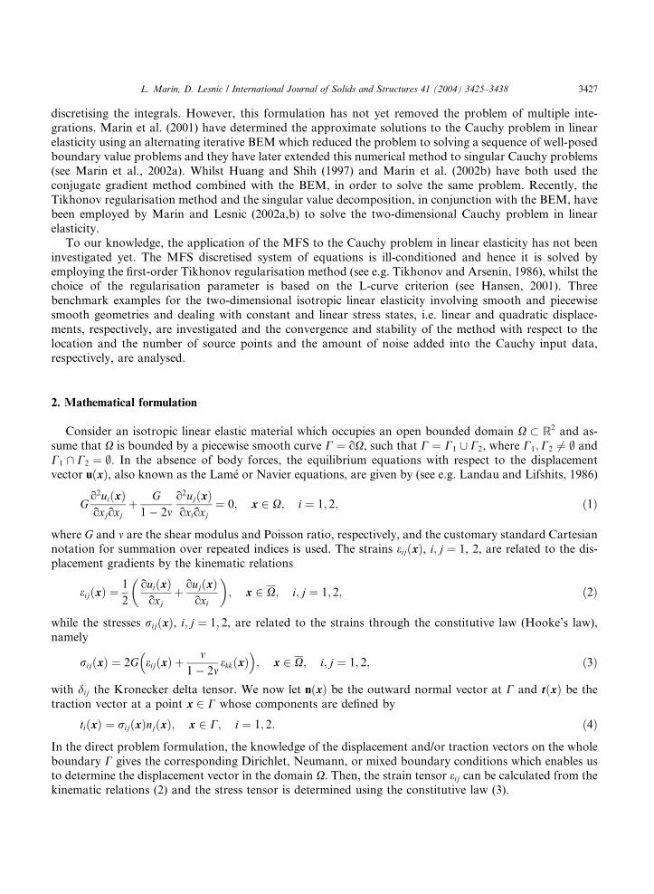
values as the number M of source points increases. A similar conclusion can be drawn from Fig. 7(a) and(b) which present the numerical solutions for the displacement u1 on the underspecified boundary x1 ¼ 1
and the traction t2 on the underspecified boundary x2 ¼ 1, respectively, obtained for Example 2 with
various numbers of source points, namely M 2 f5; 10; 15; 20g, in comparison with their analytical values.
From Fig. 5–7 it can be seen that the MFS in conjunction with the first-order Tikhonov regularisation
method provides accurate and convergent numerical solutions with respect to increasing the number of
source points, with the mention that a small number of source points is required in order for the accuracy of
the numerical displacements and tractions to be achieved.
(a) (b)
Fig. 7. (a) The analytical uðanÞ1 (––) and the numerical uðkÞ1 displacements on the underspecified boundary x2 ¼ 1, and (b) the analytical
tðanÞ2 (––) and the numerical tðkÞ2 tractions on the underspecified boundary x1 ¼ 1, retrieved with N ¼ 80 boundary collocation points,
R ¼ 5:0, k ¼ kopt, pu ¼ 3% and various numbers of source points, namely M ¼ 5 (–�–), M ¼ 10 (–�–), M ¼ 15 (–M–) and M ¼ 20
(–*–), for the Example 2.
(a) (b)
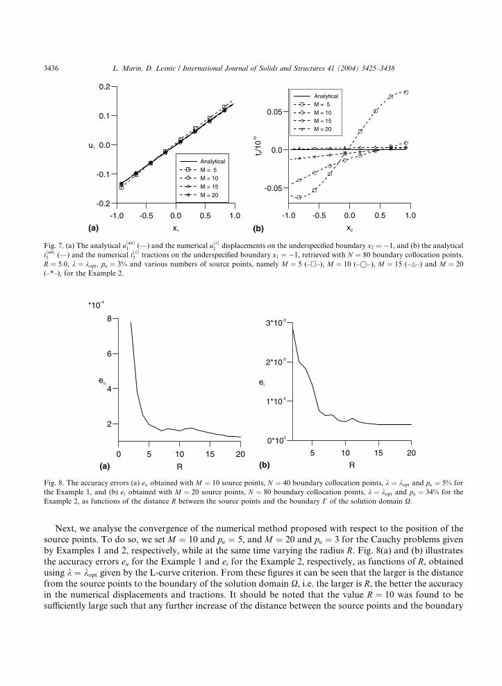
Fig. 8. The accuracy errors (a) eu obtained with M ¼ 10 source points, N ¼ 40 boundary collocation points, k ¼ kopt and pu ¼ 5% for
the Example 1, and (b) et obtained with M ¼ 20 source points, N ¼ 80 boundary collocation points, k ¼ kopt and pu ¼ 34% for the
Example 2, as functions of the distance R between the source points and the boundary C of the solution domain X.
3436 L. Marin, D. Lesnic / International Journal of Solids and Structures 41 (2004) 3425–3438
Next, we analyse the convergence of the numerical method proposed with respect to the position of thesource points. To do so, we set M ¼ 10 and pu ¼ 5, and M ¼ 20 and pu ¼ 3 for the Cauchy problems given
by Examples 1 and 2, respectively, while at the same time varying the radius R. Fig. 8(a) and (b) illustrates
the accuracy errors eu for the Example 1 and et for the Example 2, respectively, as functions of R, obtainedusing k ¼ kopt given by the L-curve criterion. From these figures it can be seen that the larger is the distance
from the source points to the boundary of the solution domain X, i.e. the larger is R, the better the accuracy
in the numerical displacements and tractions. It should be noted that the value R ¼ 10 was found to be
sufficiently large such that any further increase of the distance between the source points and the boundary

L. Marin, D. Lesnic / International Journal of Solids and Structures 41 (2004) 3425–3438 3437
C did not significantly improve the accuracy of the numerical solutions for the examples tested in this paper.
However, the optimal choice of R still remains an open problem, as pointed out by Katsurada and
Okamoto (1996), and it requires further research.
5. Conclusions
In this paper, the Cauchy problem in two-dimensional isotropic linear elasticity has been investigated by
employing the MFS. The resulting ill-conditioned system of linear algebraic equations has been regularised
by using the first-order Tikhonov regularisation method, while the choice of the optimal regularisation
parameter was based on the L-curve criterion. Three benchmark examples involving smooth and piecewise
smooth geometries and dealing with constant and linear stress states, i.e. linear and quadratic displace-
ments, respectively, have been analysed. The numerical results obtained show that the proposed method isconvergent with respect to increasing the number of source points and the distance from the source points
to the boundary of the solution domain and stable with respect to decreasing the amount of noise added
into the input data. Moreover, the method is efficient, easy to adapt to three-dimensional Cauchy problems
in linear elasticity, as well as to irregular domains and stress concentration problems, but these investi-
gations are deferred to future work.
Acknowledgements
L. Marin would like to acknowledge the financial support received from the EPSRC. The authors wouldlike to thank Dr. L. Elliott and Prof. D.B. Ingham from the Department of Applied Mathematics at the
University of Leeds for all their encouragement in performing this research work. The authors would also
like to thank the referees for their constructive suggestions.
References
Balakrishnan, K., Ramachandran, P.A., 1999. A particular solution Trefftz method for non-linear Poisson problems in heat and mass
transfer. Journal of Computational Physics 150, 239–267.
Balakrishnan, K., Sureshkumar, R., Ramachandran, P.A., 2002. An operator splitting-radial basis function method for the solution of
transient nonlinear Poisson problems. Computers and Mathematics with Applications 43, 289–304.
Berger, J.A., Karageorghis, A., 1999. The method of fundamental solutions for heat conduction in layered materials. International
Journal for Numerical Methods in Engineering 45, 1681–1694.
Berger, J.A., Karageorghis, A., 2001. The method of fundamental solutions for layered elastic materials. Engineering Analysis with
Boundary Elements 25, 877–886.
Fairweather, G., Karageorghis, A., 1998. The method of fundamental solutions for elliptic boundary value problems. Advances in
Computational Mathematics 9, 69–95.
Golberg, M.A., Chen, C.S., 1996. Discrete Projection Methods for Integral Equations. Computational Mechanics Publications,
Southampton.
Golberg, M.A., Chen, C.S., 1999. The method of fundamental solutions for potential, Helmholtz and diffusion problems. In: Golberg,
M.A. (Ed.), Boundary Integral Methods: Numerical and Mathematical Aspects. WIT Press and Computational Mechanics
Publications, Boston, pp. 105–176.
Hadamard, J., 1923. Lectures on Cauchy Problem in Linear Partial Differential Equations. Oxford University Press, London.
Hanke, M., 1996. Limitations of the L-curve method in ill-posed problems. BIT 36, 287–301.
Hansen, P.C., 1998. Rank-deficient and discrete ill-posed problems: Numerical aspects of linear inversion. SIAM, Philadelphia.
Hansen, P.C., 2001. The L-curve and its use in the numerical treatment of inverse problems. In: Johnston, P. (Ed.), Computational
Inverse Problems in Electrocardiology. WIT Press, Southampton, pp. 119–142.
3438 L. Marin, D. Lesnic / International Journal of Solids and Structures 41 (2004) 3425–3438
Huang, C.H., Shih, W.Y., 1997. A boundary element based solution of an inverse elasticity problem by conjugate gradient and
regularization method. In: Proceedings of the 7th International Offshore Polar Engineering Conference, Honolulu, USA, pp. 338–
395.
Karageorghis, A., 2001. The method of fundamental solutions for the calculation of the eigenvalues of the Helmholtz equation.
Applied Mathematics Letters 14, 837–842.
Karageorghis, A., Fairweather, G., 1987. The method of fundamental solutions for the numerical solution of the biharmonic equation.
Journal of Computational Physics 69, 434–459.
Karageorghis, A., Fairweather, G., 2000. The method of fundamental solutions for axisymmetric elasticity problems. Computational
Mechanics 25, 524–532.
Katsurada, M., Okamoto, H., 1996. The collocation points of the fundamental solution method for the potential problem. Computers
and Mathematics with Applications 31, 123–137.
Knops, R.J., Payne, L.E., 1986. Uniqueness Theorems in Linear Elasticity. Pergamon Press, Oxford.
Koya, T., Yeih, W.C., Mura, T., 1993. An inverse problem in elasticity with partially overspecified boundary conditions. II. Numerical
details. ASME Journal of Applied Mechanics 60, 601–606.
Kupradze, V.D., Aleksidze, M.A., 1964. The method of functional equations for the approximate solution of certain boundary value
problems. USSR Computational Mathematics and Mathematical Physics 4, 82–126.
Landau, L.D., Lifshits, E.M., 1986. Theory of Elasticity. Pergamon Press, Oxford.
Marin, L., Elliott, L., Ingham, D.B., Lesnic, D., 2001. Boundary element method for the Cauchy problem in linear elasticity.
Engineering Analysis with Boundary Elements 25, 783–793.
Marin, L., Elliott, L., Ingham, D.B., Lesnic, D., 2002a. An alternating boundary element algorithm for a singular Cauchy problem in
linear elasticity. Computational Mechanics 28, 479–488.
Marin, L., H�ao, D.N., Lesnic, D., 2002b. Conjugate gradient-boundary element method for the Cauchy problem in elasticity.
Quarterly Journal of Mechanics and Applied Mathematics 55, 227–247.
Marin, L., Lesnic, D., 2002a. Regularized boundary element solution for an inverse boundary value problem in linear elasticity.
Communications in Numerical Methods in Engineering 18, 817–825.
Marin, L., Lesnic, D., 2002b. Boundary element solution for the Cauchy problem in linear elasticity using singular value
decomposition. Computer Methods in Applied Mechanics and Engineering 191, 3257–3270.
Mathon, R., Johnston, R.L., 1977. The approximate solution of elliptic boundary value problems by fundamental solutions. SIAM
Journal on Numerical Analysis 14, 638–650.
Poullikkas, A., Karageorghis, A., Georgiou, G., 1998a. Methods of fundamental solutions for harmonic and biharmonic boundary
value problems. Computational Mechanics 21, 416–423.
Poullikkas, A., Karageorghis, A., Georgiou, G., 1998b. The method of fundamental solutions for inhomogeneous elliptic problems.
Computational Mechanics 22, 100–107.
Poullikkas, A., Karageorghis, A., Georgiou, G., 2001. The numerical solution of three-dimensional Signorini problems with the
method of fundamental solutions. Engineering Analysis with Boundary Elements 25, 221–227.
Poullikkas, A., Karageorghis, A., Georgiou, G., 2002. The numerical solution for three-dimensional elastostatics problems. Computers
and Structures 80, 365–370.
Ramachandran, P.A., 2002. Method of fundamental solutions: Singular value decomposition analysis. Communications in Numerical
Methods in Engineering 18, 789–801.
Tikhonov, A.N., Arsenin, V.Y., 1986. Methods for Solving Ill-posed Problems. Nauka, Moscow.
Tikhonov, A.N., Leonov, A.S., Yagola, A.G., 1998. Nonlinear Ill-posed Problems. Chapman & Hall, London.
Vogel, C.R., 1996. Non-convergence of the L-curve regularization parameter selection method. Inverse Problems 12, 535–547.
Yeih, W.C., Koya, T., Mura, T., 1993. An inverse problem in elasticity with partially overspecified boundary conditions. I. Theoretical
approach. ASME Journal of Applied Mechanics 60, 595–600.