A new low-cost meshfree method for two and threedimensional problems in elasticity

D. Mirzaeia

aDepartment of Mathematics, University of Isfahan, 81745-163 Isfahan, Iran.

Abstract

In this paper, we develop a new meshless method based on the generalized moving

least squares approximation for elasto-static problems. It is called Direct Meshless Local

Petrov-Galerkin (DMLPG) method. The most significant advantage of the new method

in comparison with the original MLPG lies on the complexity side, where DMLPG re-

duces the computational costs, significantly. Although, the “Petrov-Galerkin” strategy

is used to build up the primary local weak forms, but finally the role of trial space is

ignored and direct approximations for local weak forms and boundary conditions are

performed to construct the final stiffness matrix. This modification shifts the numerical

integrations over polynomials rather than over complicated MLS shape functions. In this

paper, DMLPG is applied for two and three dimensional problems in elasticity. Some

variations of new method are developed and their efficiencies are reported. Finally, we

will conclude that DMLPG can replace the original MLPG in many situations.

Key words: DMLPG methods, MLPG methods, MLS approximation, GMLS

approximation, Direct approximation, Elasticity problems

1. Introduction

The Meshless Local Petrov-Galerkin (MLPG) methods were widely applied to find

the numerical solutions of elasto-static and elasto-dynamic problems. MLPG was first

introduced in [1], and was first applied for elasticity in [2]. Afterward, many papers

were appeared for different types of mechanical problems. For example see [3, 4, 5, 6].

MLPG is based on local weak forms and it is known as a truly meshless method, because

it uses no global background mesh to evaluate integrals and everything breaks down to

some regular, well-shaped and independent sub-domains. This is in contrast to methods

which are based on global weak forms, such as Element-free Galerkin (EFG) method [7],

where triangulation is again required for numerical integration. But MLPG still suffers

Email address: d.mirzaei@sci.ui.ac.ir (D. Mirzaei)

Preprint submitted to ... February 11, 2014

arX

iv:1

402.

2171

v1 [

mat

h.N

A]

10

Feb

2014

from the cost of numerical integration. This is due to the complexity of the integrands.

In MLPG and all MLS based methods, integrations are down over complicated MLS

shape functions, and this leads to high computational costs in comparison with the finite

elements method (FEM), where integrands are simple and close form polynomials. There

are some researches concerning the numerical integration and trying to give accurate and

fast quadratures for MLPG. For example see [8, 9]. This is the reason why this method,

and of course the other meshless methods, have found very limited application to three-

dimensional problems, which are routine applications of FEM.

A tricky modification has been applied to MLPG in [10], which shifts the numerical

integrations over low-degree polynomial basis functions rather than complicated MLS

shape functions. This reduces the computational costs of MLPG, significantly. In the

new method, local weak forms are considered as functionals and directly approximated

from nodal data using a generalized moving least squares (GMLS) approximation. Thus

this method is called Direct MLPG (DMLPG). Although DMLPG uses the same local

forms, but it is theoretically different form MLPG, because it eliminates the role of trial

space. DMLPG can be considered as a generalized finite difference method (GFDM), not

only in its usual strong form, but also in a weak formulation. It is worthy to note that,

by this modification we do not lose the order of convergence. This has been analytically

proven in [11, 12] for different definitions of functionals, specially for the local weak forms

of DMLPG.

DMLPG has been applied to the heat conduction problem in [13] and has been

numerically investigated for 2D and 3D potential problems in [14].

In this paper, the application of DMLPG is provided for elasto-static problems for the

first time. We consider both two and three dimensional problems to show the efficiency

of the new method. The paper is written is an engineering-oriented style, and can be

easily extended to the other problems in elasticity.

2. Generalized moving least squares

Generalized moving least squares (GMLS) approximation was presented in [11] in

details. Here we briefly discuss this concept. Let Ω be a bounded subset in Rd, d ∈ Z+,

and X = x1, x2, . . . , xN ⊂ Ω be a set of meshless points scattered (with certain quality)

over Ω. The MLS method approximates the function u ∈ U (with certain smoothness)

by its values at points xj , j = 1, . . . , N , by

u(x) ≈ u(x) =

N∑j=1

aj(x)u(xj), x ∈ Ω, (2.1)

where aj(x) are MLS shape functions obtained in such way that u be the best approxima-

tion of u in polynomial subspace Pm(Rd) = spanp1, . . . , pQ, Q =(m+dd

), with respect

2

to a weighted, discrete and moving `2 norm. The weight function governs the influence

of the data points and assumed to be a function w : Ω× Ω→ R which becomes smaller

the further away its arguments are from each other. Ideally, w vanishes for arguments

x, y ∈ Ω with ‖x − y‖2 greater than a certain threshold, say δ. Such a behavior can be

modeled by using a translation-invariant weight function. This means that w is of the

form w(x, y) = ϕ(‖x − y‖2/δ) where ϕ is a compactly supported function supported in

[0, 1]. If we define

P = P (x) =(pk(xj)

)∈ RN×Q,

W = W (x) = diagw(xj , x) ∈ RN×N ,(2.2)

then a simple calculation gives the shape functions

a(x) := [a1(x), . . . , aN (x)] = p(x)(PTWP )−1PTW. (2.3)

where p = [p1, . . . , pQ]. If Xx = xj : ‖x − xj‖ 6 δ is Pm(Rd)-unisolvent then A(x) =

PTWP is positive definite [15] and the MLS approximation is well-defined at sample

point x. Of course if ‖x − xj‖ > δ then aj(x) = 0. Thus, in programming we can

only form P and W for active points Xx instead of X. Derivatives of u are usually

approximated by derivatives of u,

Dαu(x) ≈ Dαu(x) =

N∑j=1

Dαaj(x)u(xj), x ∈ Ω, α = (α1, . . . , αd) ∈ Nd0. (2.4)

These derivatives are sometimes called standard or full derivatives. Details are in [16, 17]

and any other text containing the application of MLS approximation.

The GMLS approximation can be introduced as bellow. Suppose that λ is a linear

functional from the dual space U∗. The problem is the recovery of λ(u) from nodal values

u(x1), . . . , u(xN ). The functional λ can, for instance, describe point evaluations of u, its

derivatives up to order m, and the weak formulations which involve u or a derivative

against some test function. The approximation λ(u) of λ(u) should be a linear function

of the data u(xj), i.e., it should have the form

λ(u) ≈ λ(u) =

N∑j=1

aj(λ)u(xj), (2.5)

where aj(λ) are shape functions associated to the functional λ. If λ is chosen to be the

point evaluation functional δx, where δx(u) := u(x), then the classical MLS approxima-

tion (2.1) is resulted. If we assume λ is finally evaluated at sample point x, then the same

weight function w(x, y) as in the classical MLS can be used independent of the choice of

λ. Using this assumption, analogous to (2.3), [11] proves,

a(λ) := [a1(λ), . . . , aN (λ)] = λ(P)(PTWP )−1PTW, (2.6)3

where λ(P) = [λ(p1), . . . , λ(pQ)]. In fact, we have a direct approximation for λ(u) from

nodal values u(x1), . . . , u(xN ), without any detour via classical MLS shape functions.

One can see, λ acts only on polynomial basis functions. This is the central idea in this

GMLS approximation which finally speeds up our numerical algorithms. If λ contains

derivatives of u, (2.6) shows that derivatives of weight functions are not required. This

paves the way for generalizing the forthcoming schemes for discontinuous problems.

In particular, if λ(u) = Dα(u) then derivatives of u are recovered. They are different

from the standard derivatives (2.4), and in meshless literatures are called diffuse or

uncertain derivatives. But [11] and [12] prove the optimal rate of convergence for them

toward the exact derivatives, and thus there is no diffuse or uncertain about them. As

suggested in [11], they can be called GMLS derivative approximations.

In next sections, we deliberately choose λ in such way that MLPG methods speed

up, significantly.

The GMLS approximation of this section is different from one presented in [18]. In

that paper a Hermite-type MLS approximation has been used to solve the forth order

problems of thin beams. Here we approximate the general functional λ(u) from values

u(x1), . . . , u(xN ), where information of Dαu is not required. In more general situation,

the GMLS approximation of [18] can be written as

u(x) ≈ u(x) =

K∑k=1

N∑j=1

ak,j(x)µk,j(u),

where µk,j are linear functionals from U∗ and should be chosen properly to ensure the

solvability of the problem.

In a more and more general situation, both these generalizations can be used simul-

taneously

λ(u) ≈ λ(u) =

K∑k=1

N∑j=1

ak,j(λ)µk,j(u).

Up to the now, there is no rigorous error analysis for such generalized approximation,

even when λ and µk,j are some special functionals. Throughout, we leave the above

recent formulations and focus on GMLS approximation (2.5) together with (2.6).

3. Local weak forms of the elasticity problem

Let Ω ⊂ Rd (usually d = 2, 3) is a bounded domain with boundary Γ. From here on,

integers i and j are assumed to vary from 1 to d. Consider the following d-dimensional

elasto-static problem

σij,j + bi = 0, in Ω (3.1)

4

where σij is the stress tensor, which corresponds to the displacement field ui, and bi is

the body force. The corresponding boundary conditions are given by

ui = ui, on Γu, (3.2)

ti = σijnj = ti, on Γt, (3.3)

where ui and ti are the prescribed displacement and traction on the boundaries Γu and

Γt, respectively. n is the unit outward normal to the boundary Γ.

Many numerical methods such as FEM, FVM, BEM, EFG and etc. are based on a

global weak form of (3.1) over entire Ω, which can be derived using the integration by

parts. However, the MLPG method starts from weak forms over sub-domains Ωk inside

the global domain Ω. Sub-domains usually cover the entire domain Ω and have simple

geometries in order of doing the numerical integrations as much as possible.

Let X = x1, x2, . . . , xN ⊂ Ω are scattered meshless points, where some points are

located on the boundary Γ to enforce the boundary conditions. In this work, spherical

(circular in 2D) subdomains Ωk = B(xk, rk)∩Ω with radius rk centered at xk, and cubical

(rectangular in 2D) subdomains Ωk = C(xk, sk) ∩ Ω with side-length sk centered at xk

are employed. Of course, for boundary points, ∂Ωk intersects with the global boundary

Γ. A local weak form of the equilibrium equation over Ωk is written as∫Ωk

(σij,j + bi)vi dΩ = 0, (3.4)

where vi are appropriate test functions. We are not introduced lagrange multiplier or

penalty parameter in the weak form, because in our numerical method the essential

boundary conditions are imposed in a suitable collocation form. Thus we assume xk

is located either inside Ω or on Γt where the tractions are prescribed. Using σij,jvi =

(σijvi),j − σijvi,j and the Divergence Theorem, (3.4) yields∫∂Ωk

σijnjvi dΓ−∫

Ωk

σijvi,j dΩ =

∫Ωk

bivi dΩ, (3.5)

where n is the outward unit normal to the boundary ∂Ωk. Imposing the natural boundary

conditions σijnj = ti on ∂Ωk ∩ Γt, we have∫∂Ωk\Γt

σijnjvi dΓ−∫

Ωk

σijvi,j dΩ =

∫Ωk

bivi dΩ−∫∂Ωk∩Γt

tivi dΓ. (3.6)

In Petrov-Galerkin methods, the trial functions and the test functions come from different

spaces. Thus there will be many choices for test functions vi, and this leads to a list of

MLPG methods labeled from 1 to 6. But this may cause some difficulties in mathematical

analysis. Up to the here, the new procedure is identical to the classical MLPG method.

In the next section we pave the way of going from MLPG to DMLPG using the concept

of GMLS approximation.5

4. DMLPG formulation

Although, DMLPG uses the same local weak forms obtained from a Petrov-Galerkin

formulation, but it is mathematically different from MLPG because direct approxima-

tions for local weak forms are provided to rule out the action of trial space.

Using the same labels as in MLPG, here we discuss DMLPG1 and 5 and leave the

others for a new research. Note that there are some difficulties to develop DMLPG3 and

6 because they are based on a Galerkin formulation [10, 13].

We use the same scheme to impose the the essential boundary conditions in all types

of DMLPG. The MLS collocation method is applied on points located on Γu,

N∑`=1

a`(xk)ui(x`) = ui(xk), xk ∈ Γu. (4.1)

In fact, the functional λ in GMLS is taken to be δxk, the point evaluation functionals at

xk. In following subsections, we consider the local weak forms around the points located

either inside Ω or over Neumann parts of the boundary Γ.

4.1. DMLPG1

If test functions vi are chosen such that they all vanish over ∂Ωk \ Γt, then the first

integral in (3.6) vanishes and if we define

λ(i)k (u) :=−

∫Ωk

σijvi,j dΩ,

β(i)k :=

∫Ωk

bivi dΩ−∫∂Ωk∩Γt

tivi dΓ,

xk ∈ int(Ω) ∪ Γt, (4.2)

then(3.5) becomes

λ(i)k (u) = β

(i)k , xk ∈ int(Ω) ∪ Γt.

Now, the GMLS can be applied to approximate the above functionals. To simplify the

notation, let

λk =

λ

(1)k...

λ(d)k

, βk =

β

(1)k...

β(d)k

, u =

u1

...

ud

, Ak` =

a

(11)k` · · · a

(1d)k`

.... . .

...

a(d1)k` · · · a

(dd)k`

,where A = (Ak`) is introduced as a block matrix for reserving the acts of GMLS functions.

Blocks of A are not diagonal, because λ(i)k (u) depends not only on ui (for specified i) but

also on all ui for i = 1, . . . , d. The GMLS approximation can be used to write

λk(u) ≈ λk(u) =

N∑`=1

Ak`u(x`). (4.3)

6

According to (2.6), if Ak,: represents the k-th block row of A, then

Ak,: = λk(P)Φ ∈ Rd×dN , (4.4)

where Φ ∈ RdQ×dN is a block matrix obtained form φ := (PTWP )−1WPT ∈ RQ×N by

Φij =

φij 0

. . .

0 φij

∈ Rd×d.

Matrices P and W are defined in (2.2), and

λk(P) = −[ ∫

Ωk

εvDP1(x)dΩ︸ ︷︷ ︸∈Rd×d

,

∫Ωk

εvDP2(x)dΩ︸ ︷︷ ︸∈Rd×d

, . . . ,

∫Ωk

εvDPQ(x)dΩ︸ ︷︷ ︸∈Rd×d

]∈ Rd×dQ, (4.5)

where for a two dimensional problem (d = 2) of isotropic material, the stress-strain

matrix D is defined by

D =E

1− ν2

1 ν 0

ν 1 0

0 0 (1− ν)/2

,where

E =

E for plane stress

E1−ν2 for plane strain

ν =

ν for plane stress

ν1−ν for plane strain

,

in which E and ν are Youngs modulus and Poissons ratio, respectively. The strain matrix

for test functions vi is

εv =

[v1,1 0 v1,2

0 v2,2 v2,1

],

and

Pn(x) =

pn,1(x) 0

0 pn,2(x)

pn,2(x) pn,1(x)

, n = 1, 2, . . . , Q.

For the elasticity problem of isotropic material in 3D (i.e. d = 3), we have D =[D1 0

0 D2

]∈ R6×6 where

D1 =E

(1− 2ν)(1 + ν)

1− ν ν ν

ν 1− ν ν

ν ν 1− ν

, D2 =E

2(1 + ν)

1 0 0

0 1 0

0 0 1

.

7

In addition, the strain matrix of test functions is

εv =

v1,1 0 0 0 v1,3 v1,2

0 v2,2 0 v2,3 0 v2,1

0 0 v3,3 v3,2 v3,1 0

,and finally

Pn(x) =

pn,1(x) 0 0

0 pn,2(x) 0

0 0 pn,3(x)

0 pn,3(x) pn,2(x)

pn,3(x) 0 pn,1(x)

pn,2(x) pn,1(x) 0

, n = 1, 2, . . . , Q.

For simplicity we choose v1 = · · · = vd =: v in following numerical algorithms. To set up

the final linear system, we first assume

u = [u1(x1), . . . , ud(x1), u1(x2), . . . , ud(x2), . . . , u1(xN ), . . . , ud(xN )]T ∈ RdN×1.

Without loss of generality, let the first Nb meshless points are located on Γu. The

boundary matrix B ∈ RdNb×dN corresponds to the essential boundary conditions is a

block matrix in which

Bk` =

a`(xk) 0

. . .

0 a`(xk)

d×d

,

where a`(xk) are the values of GMLS shape functions defined in (4.1). Finally if we set

K =

[B

A

]dN×dN

, R =[u(x1) · · · u(xNb) βNb+1 · · · βN

]TdN×1

,

then we have the final system of linear equations

Ku = R. (4.6)

Sometimes, in a boundary point xk both tractions and displacements are prescribed, i.e.

for some i, tractions ti and for the others, displacements ui are known. Let for such point

xk, displacements ui1 , . . . , uis for indices i1, . . . , is ⊂ 1, 2, . . . , d are prescribed. Since

the essential boundary conditions are applied using the collocation method, in the k-th

block row of A, rows i1, . . . , is should be replaced by corresponding MLS shape function

vectors, say a(im)k , 1 6 m 6 s, of size dN . These vectors are introduces as bellow: first we

define a(im)k as zero dN -vectors. Then vector [a1(xk), a2(xk), . . . , aN (xk)] of MLS shape

functions is settled down in places im, im + d, . . . , im + (N − 1)d of a(im)k . Of course the

8

corresponding right-hand sides should form by known boundary values uim instead of

β(im)k .

In DMLPG process, integrations are only appeared in (4.5), where they are done over

polynomials rather that MLS shape functions. This is the main idea behind the DMLPG

approach. In fact, DMLPG shifts the numerical integration into the MLS itself, rather

than into an outside loop over calls to MLS routines. Thus DMLPG is extremely faster

than original MLPG.

Moreover, in some situations, we can get the exact numerical integrations with limited

number of Gaussian points. For example, if cubical subdomains with polynomial test

function v are used in DMLPG1, the integrands are d-variate polynomials of degree (m−1)×(n−1), where n is the degree of the polynomial test function. Thus a

⌈(m−1)(n−1)+1

2

⌉–

point Gauss quadrature in each axis is enough for doing the exact numerical integration.

As a polynomial test function on the square or cube for DMLPG1 with n = 2, we can

use

v = v(x;xk) =

∏di=1

(1− 4

s2k(χi − χki)

2), x ∈ C(xk, sk),

0, otherwise(4.7)

where x = (χ1, . . . , χd) and xk = (χk1, . . . , χkd). Note that, we should be careful for

points located on the curved parts of the boundary.

4.2. DMLPG5

If v = vi ≡ 1 are chosen over Ωk, then the second integral in (3.6) vanishes, and by

defining

λ(i)k (u) :=

∫∂Ωk\Γt

σijnj dΓ, β(i)k =

∫Ωk

bidΩ−∫∂Ωk∩Γt

ti dΓ, xk ∈ int(Ω) ∪ Γt, (4.8)

we have

λ(i)k (u) = β

(i)k .

As before, we apply the GMLS to find direct approximations for functionals λ(i)k . Equa-

tions are the same as those where obtained for DMLPG1, unless (4.5) which should be

replaced by

λk(P) =[ ∫

∂Ωk\Γt

NDP1(x)dΓ,

∫∂Ωk\Γt

NDP2(x)dΓ, . . . ,

∫∂Ωk\Γt

NDPQ(x)dΓ]∈ Rd×dQ,

(4.9)

where N is reserved for matrix of components of normal vector, which is defined for two

dimensional problem by

N =

[n1 0 n2

0 n2 n1

],

9

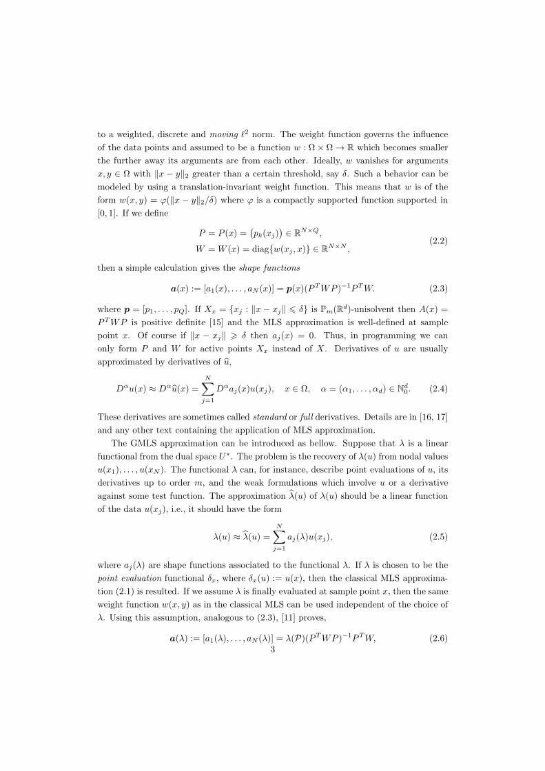
and for three dimensional problem by

N =

n1 0 0 0 n3 n2

0 n2 0 n3 0 n1

0 0 n3 n2 n1 0

.One can see, the integrals in (4.9) are all boundary integrals. Thus DMLPG5 is even

faster. Again if cubes are used as subdomains, a⌈m2

⌉–point Gauss quadrature in each

axis gives the exact solution for local boundary integrals.

In the following section, some numerical experiments in two and three dimensional

elasticity are presented to show the efficiencies of new methods.

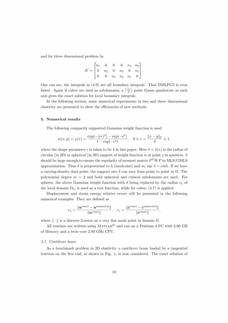
5. Numerical results

The following compactly supported Gaussian weight function is used

w(x, y) = ϕ(r) =exp(−(εr)2)− exp(−ε2)

1− exp(−ε2), 0 6 r =

‖x− y‖2δ

6 1,

where the shape parameter ε is taken to be 4 in this paper. Here δ = δ(x) is the radius of

circular (in 2D) or spherical (in 3D) support of weight function w at point x in question. δ

should be large enough to ensure the regularity of moment matrix PTWP in MLS/GMLS

approximation. Thus δ is proportional to h (mesh-size) and m, say δ = cmh. If we have

a varying-density data point, the support size δ can vary from point to point in Ω. The

polynomial degree m = 2 and both spherical and cubical subdomains are used. For

spheres, the above Gaussian weight function with δ being replaced by the radius rk of

the local domain Ωk, is used as a test function, while for cubes, (4.7) is applied.

Displacement and strain energy relative errors will be presented in the following

numerical examples. They are defined as

ru =‖uexact − unumerical‖

‖uexact‖, rε =

‖εexact − εnumerical‖‖εexact‖

,

where ‖ · ‖ is a discrete 2-norm on a very fine mesh point in domain Ω.

All routines are written using Matlab c© and run on a Pentium 4 PC with 2.00 GB

of Memory and a twin–core 2.80 GHz CPU.

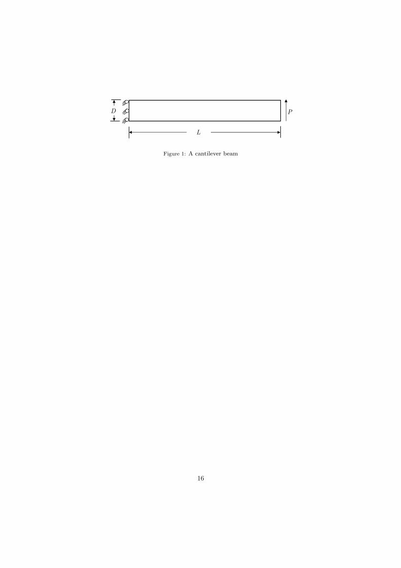
5.1. Cantilever beam

As a benchmark problem in 2D elasticity, a cantilever beam loaded by a tangential

traction on the free end, as shown in Fig. 1, is now considered. The exact solution of

10

this problem is given in Timoshenko and Goodier [19] as follow:

u1 = − P

6EI

(χ2 −

D

2

)(3χ1(2L− χ1) + (2 + ν)χ2(χ2 −D)

),

u2 =P

6EI

[χ

21(3L− χ1) + 3ν(L− χ1)

(χ2 −

D

2

)2

+4 + 5ν

4D2

χ1

],

where I = D3/12 and x = (χ1, χ2) ∈ R2. The corresponding exact stresses are

σ11 = −PI

(L− χ1)

(χ2 −

D

2

),

σ22 = 0,

σ12 = −Pχ2

2I(χ2 −D) .

Both MLPG1 and DMLPG1 are applied with L = 8, D = 1, P = 1, E = 1, ν = 0.25 for

the plane stress case. The uniform mesh sizes (33× 5), (65× 9) and (129× 17) are used

to detect the rates of convergence and computational costs of both techniques. Circular

domains with radius rk = 0.7h, and rectangular domains with hight-length h × h are

employed as sub-domains Ωk for all k. As pointed before, for m = 2 a 2-point Gaussian

quadrature in each axis is enough to get the exact numerical integrations over rectangles

in DMLPG. But 10-point quadrature in each axis is used for circles (r and θ directions) in

both methods and rectangles in MLPG. The sufficiently large number of Gaussian points

should be used to get the high accuracy for integration against MLS shape functions in

MLPG. However, DMLPG works properly with fewer integration points, because there

is no shape function incorporated in integrands. Here, to perform the comparisons in

complexity side, we use the same number of Gaussian points for both methods with

circular subdomains. Results are presented in Figs. 2 and 3 to compare the accuracy of

numerical displacements, numerical stains in MLPG1 and DMLPG1 for rectangular and

circular sub-domains. The rates are more or less the same, but the results of DMLPG

with rectangles are surprising, because we have exact numerical integration.

As discussed, DMLPG is superior to MLPG in complexity side. To confirm this

numerically, the CUP times used are compared in Fig. 4 for rectangular and circular

subdomains.

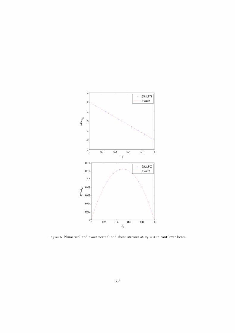
Finally, the DMLPG solutions of normal stress σ11 and shear stress σ12 at χ1 = L/2 =

4 are plotted in Fig. 5 and compared with the exact solutions.

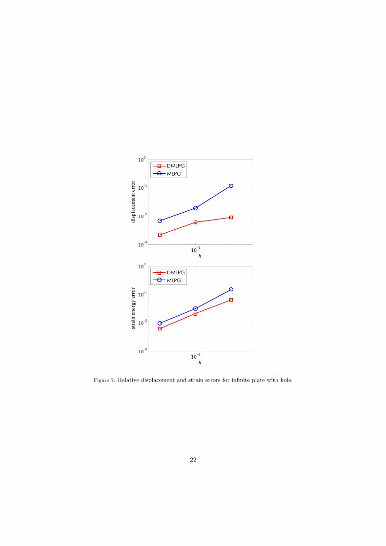
5.2. Infinite plate with circular hole

Consider an infinite plate with a central hole χ21 + χ2

2 6 a2 of radius a, subjected to a

unidirectional tensile load of σ = 1 in the χ1-direction at infinity. There is an analytical

11

solution for stress in the polar coordinate (r, θ)

σ11 =σ

[1− a2

r2

(3

2cos 2θ + cos 4θ

)+

3a4

2r4cos 4θ

],

σ12 =σ

[−a

2

r2

(1

2sin 2θ + sin 4θ

)+

3a4

2r4sin 4θ

],

σ22 =σ

[−a

2

r2

(1

2cos 2θ − cos 4θ

)− 3a4

2r4cos 4θ

],

with the corresponding displacements

u1 =1 + ν

Eσ

[1

1 + νr cos θ +

2

1 + ν

a2

rcos θ +

1

2

a2

rcos 3θ − 1

2

a4

r3cos 3θ

],

u2 =1 + ν

Eσ

[−ν

1 + νr sin θ − 1− ν

1 + ν

a2

rsin θ +

1

2

a2

rsin 3θ − 1

2

a4

r3sin 3θ

].

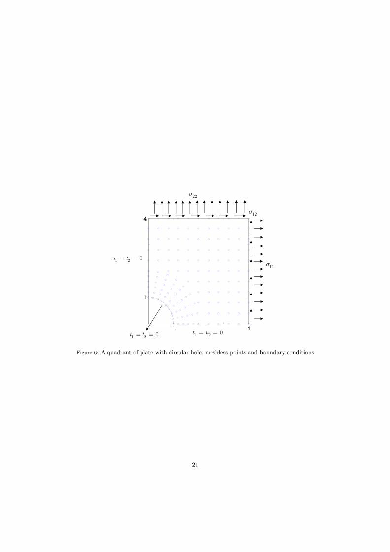
In computations, we consider a finite plate of length b = 4 with a circular hole of radius

a = 1 (see Fig. 6), where the solution is very close to that of the infinite plate [20].

Due to symmetry, only the upper right quadrant of the plate is modelled. The traction

boundary conditions given by the exact solution are imposed on the right and top edges

(see Fig. 6). Symmetry conditions are imposed on the left and bottom edges, i.e.,

u1 = 0, t2 = 0 are prescribed on the left edge and u2 = 0, t1 = 0 on the bottom edge,

and the inner boundary at a = 1 is traction free, i.e. t1 = t2 = 0. Numerical results

are presented for a plane stress case with E = 1.0 and ν = 0.25. The initial set point

is depicted in Fig. 6, where we use more points near the hole. Thus the support size δ

varies according to the density of neighboring points. Here δ = 2mh and δ = 2.5mh are

used for points near the hole and points far away from the hole, respectively. Mesh-size

h is defined to be minhr, hθ for near points. In DMLPG, we use circular subdomains

for points located on the arc boundary r = a, and square subdomains for other points.

Computations are repeated by halving hr and hθ, twice. Results are presented in Figs.

7 and 8 which compare the displacement errors, the strain energy errors, and the CPU

times used. Moreover, the exact normal stress σ11 at χ1 = 0 is plotted in Fig. 9 and

compared with the DMLPG solution.

5.3. 3D Boussinesq problem

The Boussinesq problem can be describe as a concentrated load acting on a semi-

infinite elastic medium with no body force. The exact displacement field within the

semi-infinite medium is given by Timoshenko and Goodier [19]

ur =(1 + ν)P

2Eπρ

[zr

ρ2− (1− 2ν)r

ρ+ z

],

w =(1 + ν)P

2Eπρ

[z2

ρ2+ 2(1− ν)

].

12

where ur is the radial displacement, w (or u3) is the vertical displacement, ρ =√χ2

1 + χ22 + χ2

3

is the distance to the loading point and r =√χ2

1 + χ22 is the projection of ρ on the loading

surface. The exact stresses field is

σr =P

2πρ2

[−3zr2

ρ3+

(1− 2ν)ρ

ρ+ z

],

σθ =(1− 2ν)P

2πρ2

[z

ρ− ρ

ρ+ z

],

σzz = −3πz3

2πρ5,

τzr = τrz = −3πrz2

2πρ5.

It is clear that the displacements and stresses are strongly singular and approach to

infinity; with the displacement being O(1/ρ) and the stresses being O(1/ρ2). MLPG has

been applied to this problem in [3].

In numerical simulation, a finite sphere with large radius b = 10 is used. Due to

the symmetry, a first one-eighth of the sphere is considered and symmetry boundary

conditions are applied on planes xz and yz (see Fig. 10). In fact we impose t1 = u2 = t3 =

0 on plane xz, and u1 = t2 = t3 = 0 on plane yz. In order to avoid direct encounter with

the singular loading point, the theoretical displacement is applied on a small spherical

surface with radius b/40 = 0.25. An isotropic material of E = 1000, ν = 0.25 and P = 1

is used. The number of meshless points is 1386, which are scattered inside the domain

and on the boundary. The density of nodes depends on the distance from the loading

points, where we have many points near the small sphere and few points far from it (see

Fig. 10). Thus the support size δ varies and depends on ρ, correspondingly. Analytical

and DMLPG solutions of the radial displacement ur and vertical displacement w on the

surface xy are plotted in Fig. 11. The Von Mises stress on the surface xy is also shown

in Fig. 12. These are the results of DMLPG1 with cubes as sub-domains where the CPU

time used is around 5 seconds. Again we note that a 2-point Gaussian quadrature in

each axis gives the exact numerical integration. The same results will be obtained by

DMLPG5.

Finally, for comparison we apply both MLPG1 and MLPG5 to this problem with the

same meshless points and MLS parameters. The accuracy of results are far less than

DMLPG solutions and the CPU run times are about 7400 sec. for MLPG1 and 450 sec.

for MLPG5. In computations, a 10-point Gauss formula is employed in each axis. In

fact, for MLPG1, the MLS shape function subroutines should be called 1000 times to

integrate over a sub-domain Ωk. In MLPG5 this number reduces to 100, because the

integrals are all boundary integrals in this example. Compare with DMLPG where the

MLS subroutines are not called for integrations at all, leading to 5 sec. running time in

this example.13

6. Conclusion

In this paper we developed a new meshfree method for elasticity problems, which is

a weak form method in the cost-level of collocation (integration-free) methods. Integra-

tions have been shifted into the MLS itself, rather than into an outside loop over calls to

MLS routines. In fact, we need to integrate against low-degree polynomials basis func-

tions instead of complicated MLS shape functions. Besides, in some situations we can

perform exact numerical integrations. We applied DMLPG1 and 5 for problems in two

and three dimensional elasticity in this paper. The new methods can be easily applied

to other problems in solid engineering. On a downside, DMLPG1 and 5 do not work for

linear basis functions (m = 1). In addition, because of symmetry properties of polyno-

mials in local sub-domains, [10] shows that the convergence rates do not increase when

going from m = 2k to m = 2k + 1. But the results show that this observation affects

MLPG and DMLPG in the same way. DMLPG4 can be formulated using the strategy

presented in [21] to make the second unsymmetric local weak forms and then applying

the GMLS approximation of this paper. Finally, we believe that DMLPG methods have

great potential to replace the original MLPG methods in many situations, specially for

three dimensional problems.

Acknowledgment

Special thanks go to Prof. R. Schaback, Universitat Gottingen and Dr. K. Hasanpour,

Department of Mechanical Engineering, University of Isfahan, for their useful helps and

comments.

References

[1] Atluri S, Zhu TL. A new meshless local Petrov-Galerkin (MLPG) approach in computational me-

chanics. Computational Mechanics 1998; 22:117–127.

[2] Atluri SN, Zhu TL. The meshless local Petrov-Galerkin (MLPG) approach for solving problems in

elasto-statics. Computational Mechanics 2000; 25:169–179.

[3] Li Q, Shen S, Han ZD, Atluri SN. Application of meshless local Petrov-Galerkin (MLPG) to prob-

lems with singularities, and material discontinuities, in 3-D elasticity. CMES: Computer Modeling

in Engineering & Scineces 2003; 4:571–585.

[4] Soares Jr D, Sladek V, Sladek J. Modified meshless local PetrovGalerkin formulations for elastody-

namics. International Journal for Numerical Methods in Engineering 2012; 90:1508–1828.

[5] Sladek J, Sladek V, Zhang C, Krivacek J, Wen PH. Analysis of orthotropic thick plates by meshless

local Petrov-Galerkin (MLPG) method. International Journal for Numerical Methods in Engineer-

ing 2006; 67:1830–1850.

[6] Gu YT, Liu GR. A meshless local Petrov-Galerkin (MLPG) method for free and forced vibration

analyses for solids. Computational Mechanics 2001; 27:188–198.

[7] Belytschko T, Lu Y, Gu L. Element-Free Galerkin methods. International Journal for Numerical

Methods in Engineering 1994; 37:229–256.

14

[8] Pecher R. Efficient cubature formulae for MLPG and related methods. International Journal for

Numerical Methods in Engineering 2006; 65:566–593.

[9] Mazzia A, Pini G. Product Gauss quadrature rules vs. cubature rules in the meshless local Petrov-

Galerkin method. Journal of Complexity 2010; 26:82–101.

[10] Mirzaei D, Schaback R. Direct Meshless Local Petrov-Galerkin (DMLPG) method: a generalized

MLS approximation. Applied Numerical Mathematics 2013; 33:73–82.

[11] Mirzaei D, Schaback R, Dehghan M. On generalized moving least squares and diffuse derivatives.

IMA Journal of Numerical Analysis 2012; 32:983–1000.

[12] Mirzaei D. Error boounds for GMLS derivatives approximations in Lp norms 2013. Preprint, Uni-

versity of Isfahan, Available at http://sci.ui.ac.ir/~d.mirzaei.

[13] Mirzaei D, Schaback R. Sovling heat conduction problem by the Direct Meshless Local Petrov-

Galerkin (DMLPG) method. Numerical Algorithms 2013; In press.

[14] Mazzia A, Pini G, Sartoretto F. Numerical investigation on direct MLPG for 2D and 3D potential

problems. Computer Modeling & Simulation in Engineering 2012; 88:183–209.

[15] Wendland H. Scattered Data Approximation. Cambridge University Press, 2005.

[16] Lancaster P, Salkauskas K. Surfaces generated by moving least squares methods. Mathematics of

Computation 1981; 37:141–158.

[17] Belytschko T, Krongauz Y, Organ D, Fleming M, Krysl P. Meshless methods: an overview and

recent developments. Computer Methods in Applied Mechanics and Engineering, special issue 1996;

139:3–47.

[18] Atluri SN, Cho JY, Kim HG. Analysis of thin beams, using the meshless local Petrov-Galerkin

method, with generalized moving least squares interpolations. Computational Mechanics 1999;

24:334–347.

[19] Timoshenko SP, Goodier JN. Theory of Elasticity. 3rd edition, McGraw-Hill: New York, 1970.

[20] Roark RJ, Young WC. Formulas for Stress and Strain. McGraw-Hill, 1975.

[21] Atluri SN, Sladek J, Sladek V, Zhu TL. The local boundary integral equation (LBIE) and it’s

meshless implementation for linear elasticity. Computational Mechanics 2000; 25:180–198.

15

P

L

D

Figure 1: A cantilever beam

16

10-110-4

10-3

10-2

10-1

disp

lace

men

t err

or

h

DMLPGMLPG

10-110-4

10-3

10-2

10-1

stra

in e

nerg

y er

ror

h

DMLPGMLPG

Figure 2: Relative displacement and strain errors for beam, rectangular subdomains

17

10-110-3

10-2

10-1

disp

lace

men

t err

or

h

DMLPGMLPG

10-110-3

10-2

10-1

stra

in e

nerg

y er

ror

h

DMLPGMLPG

Figure 3: Relative displacement and strain errors for beam, circular subdomains

18

0 500 1000 1500 2000 25000

100

200

300

400

500

600

CPU

tim

e us

ed (s

econ

d)

N

DMLPGMLPG

0 500 1000 1500 2000 25000

100

200

300

400

500

600

CPU

tim

e us

ed (s

econ

d)

N

DMLPGMLPG

Figure 4: Computational costs for beam, rectangular (left) and circular (right) subdomains

19

0 0.2 0.4 0.6 0.8 1-3

-2

-1

0

1

2

3

I/P

11

x2

DMLPGExact

0 0.2 0.4 0.6 0.8 10

0.02

0.04

0.06

0.08

0.1

0.12

0.14

I/P

12

x2

DMLPGExact

Figure 5: Numerical and exact normal and shear stresses at x1 = 4 in cantilever beam

20

1 4

1

412s

22s

11s

1 2 0t u= =

1 2 0u t= =

1 2 0t t= =

Figure 6: A quadrant of plate with circular hole, meshless points and boundary conditions

21

10-110-3

10-2

10-1

100

disp

lace

men

t err

or

h

DMLPGMLPG

10-110-3

10-2

10-1

100

stra

in e

nerg

y er

ror

h

DMLPGMLPG

Figure 7: Relative displacement and strain errors for infinite plate with hole.

22

0 500 1000 1500 2000 2500

0

50

100

150

200

250

300

CPU

tim

e us

ed (s

econ

d)

N

DMLPGMLPG

Figure 8: Computational costs for infinite plate with hole

23

1 1.5 2 2.5 3 3.5 41

1.5

2

2.5

3

3.5

11

y

DMLPGExact

1 1.5 2 2.5 3 3.5 41

1.5

2

2.5

3

3.5

11

y

DMLPGExact

Figure 9: Numerical and exact normal stresses in plate, 535 nodes (left), 2034 nodes (right)

24

2c

3c

1c

Theoretical displacements

Theoretical displacements

1 2 3 0t u t= = =

1 2 3 0u t t= = =

0

5

10 0

5

10

0

2

4

6

8

10

Figure 10: The consideration domain and meshless points (1386 points) in Boussinesq problem

25

0 2 4 6 8 10-4

-3

-2

-1

0x 10-4

r

u r

DMLPGExact

0 2 4 6 8 100

0.2

0.4

0.6

0.8

1

1.2x 10-3

r

w

DMLPGExact

Figure 11: Radial Displacement ur and vertical displacement w in loading surface in Boussinesq

problem

26

0 2 4 6 8 100

0.5

1

1.5

2

2.5

r

VM

DMLPGExact

Figure 12: Von Mises Stress in loading surface in Boussinesq problem

27