T. Craciunescu, G. Bonheure, V. Kiptily, A. Murari, S. Soare, I. Tiseanu, V. Zoitaand JET EFDA contributors

EFDA–JET–PR(07)48

The Maximum LikelihoodReconstruction Method for JET

Neutron Tomography

“This document is intended for publication in the open literature. It is made available on theunderstanding that it may not be further circulated and extracts or references may not be publishedprior to publication of the original when applicable, or without the consent of the Publications Officer,EFDA, Culham Science Centre, Abingdon, Oxon, OX14 3DB, UK.”

“Enquiries about Copyright and reproduction should be addressed to the Publications Officer, EFDA,Culham Science Centre, Abingdon, Oxon, OX14 3DB, UK.”

The Maximum LikelihoodReconstruction Method for JET

Neutron TomographyT. Craciunescu1, G. Bonheure2, V. Kiptily3, A. Murari4, S. Soare5, I. Tiseanu1,

V. Zoita1 and JET EFDA contributors*

1EURATOM-MEdC Association, National Institute for Laser, Plasma and Radiation Physics, Bucharest, Romania2Partners in the TEC, ‘Euratom-Belgian state’ Association LPP-ERM/KMS, B 1000 Brussels, Belgium3EURATOM-UKAEA Fusion Association, Culham Science Centre, OX14 3DB, Abingdon, OXON, UK

4Consorzio RFX, Associazione ENEA-Euratom per la Fusione, Padova, Italy5EURATOM-MEdC Association, National Institute for Cryogenics and Isotopic Technologies, Rm. Valcea, Romania

* See annex of M.L. Watkins et al, “Overview of JET Results ”, (Proc. 21 st IAEA Fusion Energy Conference, Chengdu, China (2006)).

Preprint of Paper to be submitted for publication inNuclear Instruments and Methods in Physics Research Section A

JET-EFDA, Culham Science Centre, OX14 3DB, Abingdon, UK

.

1

ABSTRACT

The JET neutron profile monitor ensures coverage of the neutron emissive region that enables

tomographic reconstruction. However, due to the availability of only two projection angles and to

the coarse sampling, tomography is a limited data set problem. A reconstruction method based on

the maximum likelihood principle is developed for solving the reconstruction problem. A smoothing

operator, defined as median filtering which uses a sliding window moving along magnetic contour

lines, is used to compensate for the lack of experimental information. The method is tested on

numerically simulated phantoms with shapes characteristic for this kind of tomography. Significant

reconstructions of experimental data are reported.

1. INTRODUCTION

The JET neutron profile monitor is a unique instrument among neutron diagnostics available at

large fusion research facilities [1-3]. The profile monitor comprises two fan shaped multi-collimator

cameras, with 10 channels in the horizontal camera and 9 channels in the vertical camera. A schematic

drawing of the JET neutron emission profile monitor, showing the 19 lines of sight is presented in

Fig.1. Each line of sight is equipped with a set of three different detectors:

i) a NE213 liquid organic scintillator with Pulse Shape Discrimination (PSD) electronics for

simultaneous measurements of the 2.5MeV D-D neutrons, 14MeV D-T neutrons and γ-rays,

ii) a BC418 plastic scintillator, insensitive to γ-rays with Eγ < 10MeV for the measurements of

14MeV D-T neutrons and

iii) a CsI(Tl) scintillation detector for measuring the hard X-rays and gamma emission in the

range between 0.2 and 6MeV. The collimation can be adjusted by use of two pairs of rotatable

steel cylinders. The size of the collimation can modify the count rates in the detectors by a

factor of 20 [4]. The instrument has a time resolution currently of 10ms.

The plasma coverage can be used for neutron or γ-ray tomography but the†existence of only two

views (projections in tomographic terms) and the coarse sampling in each projection leads to a

highly limited data set tomographic problem. A number of valuable approaches have been developed

for tomographic reconstruction of the two-dimensional 2-D neutron and gamma emissivity.

A Hybrid Pixel/Analytic Algorithm (HPAA), which involves a poloidal Fourier analysis and a

radial Abel inversion, starting from outside and working inward is reported in Ref.5. During a

series of experiments with tritium in deuterium plasmas in JET, the temporal evolution and the two

dimensional (2-D) spatial profiles of the 2.5 and 14MeV neutron emissivities from D-D and D-T

fusion reactions were inferred from measurements with the JET neutron emission profile monitor

[5-6].

Ingesson [7] applied a Constrained Optimization Method (ICOM). This method was widely used

earlier for tomographic reconstructions to soft X-ray and bolometer measurements at JET. It uses

anisotropic smoothness on flux surfaces as objective function (a priori physical information about

2

the expected emission profile) and measurements as constraints. Thus, the method searches for the

emissivity distribution that is constant on flux surfaces and gently varying in the radial direction.

Instead of traditional square pixels, a grid of pyramid local basis functions are used for the

discretization of the tomographic problem [8]. ICOM was extensively used for the diagnosis of fast

ions in the JET tokamak and relevant results were reported for γ-ray [9-11] and neutron [12-

15]†tomographic emissivity reconstruction.

The Minimum Fisher Regularization (MFR), was applied to the tomographic reconstruction of

both soft X-ray and bolometric data [16-17]. In principle, the Fisher information of the unknown 2-

D distribution is minimized, while the measurements are taken into account as constraints, using

Lagrangian multipliers. Instead of treating the fully nonlinear problem, Anton et al. [16] exploited

only the central idea and achieved a minimization of the Fisher information of the unknown 2-D

distribution by several linear regularization steps. The method was used for the neutron emissivity

reconstruction and 2-D spatial distributions of D-D and D-T neutron emission in JET ELMy H-

mode plasmas with Tritium puff were reported [18-19].

The aim of this paper is to prove that the Maximum Likelihood (ML) reconstruction method,

which has been proven to work with limited data set problems [20-21], can be customized and

successfully used for JET neutron tomography, in order to provide both accurate and fast

reconstructions. The method is evaluated both on phantoms (numerically simulated distributions)

and on experimental data.

2. IMPLEMENTATION OF THE MAXIMUM LIKELIHOOD METHOD

In 2-D tomography systems, measurements are taken along lines of sight, and can essentially be

represented by line integrals; i.e. the measurement p is given by straight line integrals of the emissivity

f (x, y), where x and y are Cartesian coordinates of the plane. The emissivity function can be

appropriately discretized on a 2-D grid. For this purpose, the reconstruction area is divided into

pixels that are sufficiently small for emissivity variations within a pixel to be negligible. The

contribution matrix element ikw represents the proportion of the emission fi from pixel i accumulated

in detector k (the weighting matrix). The basic set of tomographic equations is:

(1)

where Np and Nd are the numbers of pixels and detectors, respectively. This set of linear equations

represents the linear inverse problem. It is evident that, even with exact data constraints, this inversion

cannot be uniquely performed when there are fewer data than pixels, as is generally the case in

plasma tomography.

2.1 MAXIMUM LIKELIHOOD

The ML method arose in clinical application as a promising reconstruction method with the potential

Σ d

N

iiikk Nkfwp

p

,...,2,1 ,1

=•==

3

to yield higher resolution and lower noise reconstructions than conventional methods (see e.g Refs.

22-23). It can be derived based on the principles of the Bayesian tomography. Let P represent a set

of measured projection data, and let F represent a model of the object under consideration. The goal

is to assign values to F that accurately reflect the objects being inspected from the noisy and

potentially incomplete data, P. In ML estimation, the estimated model FML is taken to be the value

of F which maximizes the likelihood, L(P|F), of observing P, assuming that F is correct. Equivalently,

and more commonly, the log-likelihood can be maximized.

More precisely, in ML tomography, it is assumed that the emission is a Poisson process and kp is

a sample from a Poisson distribution whose expected value is:

(2)

Then the probability of obtaining the measurement P ≡ pk|k = 1,...Nd if the image is F ≡ fi|i =

1,...Np (the so-called likelihood function) is:

(3)

The ML method solves the problem of evaluating F, if P is known, by selecting the particular F

which maximizes L(P|F). This is a difficult nonlinear optimization problem and until the application

of the iterative Expectation Maximization (EM) algorithm by Shepp and Vardi [24] there was no

method with known convergence properties for generating the ML solution. The iterative solution

is given by the following formula:

(4)

where fi(iter) is the reconstructed image for the iteration iter, i and j are image element indices, k and

l are projection element indices. Due to the imbricated sums in Eq. 4 the algorithm is computationally

demanding. This leads to long reconstruction times that are not acceptable for routine clinical

application. In consequence the applicability of the method in the medical field is limited. However,

for a limited data set problem, the amount of computation for solving the iterative problem is not so

time-consuming and successful results were reported for several applications. (see e.g. Refs. 25-28).

A well known characteristic of the ML algorithm is that the unconstrained maximum-likelihood

estimator has a fundamental noise artifact that worsens as the iterative algorithm climbs the likelihood

hill. Even the likelihood function is monotonically increasing with the iteration number, the best

reconstruction is obtained before irregular high amplitude patterns or global distortions arise. In

consequence, a criterion for optimal stopping of the algorithm must be introduced. We found that the

correlation coefficient between reconstructions obtained at successive iterations reaches its maximum

value for the best reconstruction. The correlation coefficient is given by the following equation:

Σ iikk

fw

ΣΠ 1

pk!L(P/F) = ×exp -

pk

iik fw iik fw k i

Σi

ikw

jlw

i(iter+1)f

j(iter)f

kp

= i(iter)f

Σl

Σk

ikwΣk

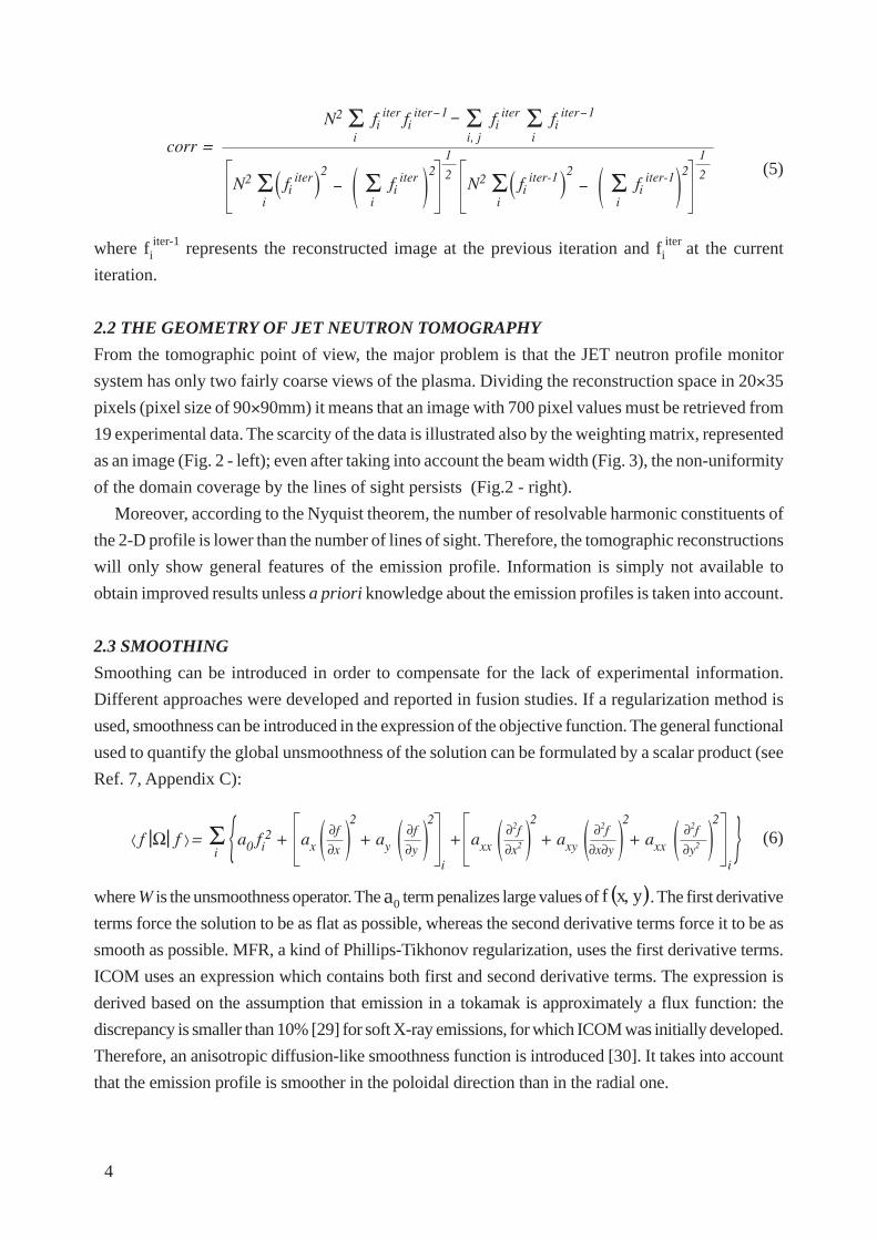
4

(5)

where fiiter-1 represents the reconstructed image at the previous iteration and fi

iter at the current

iteration.

2.2 THE GEOMETRY OF JET NEUTRON TOMOGRAPHY

From the tomographic point of view, the major problem is that the JET neutron profile monitor

system has only two fairly coarse views of the plasma. Dividing the reconstruction space in 20×35

pixels (pixel size of 90×90mm) it means that an image with 700 pixel values must be retrieved from

19 experimental data. The scarcity of the data is illustrated also by the weighting matrix, represented

as an image (Fig. 2 - left); even after taking into account the beam width (Fig. 3), the non-uniformity

of the domain coverage by the lines of sight persists (Fig.2 - right).

Moreover, according to the Nyquist theorem, the number of resolvable harmonic constituents of

the 2-D profile is lower than the number of lines of sight. Therefore, the tomographic reconstructions

will only show general features of the emission profile. Information is simply not available to

obtain improved results unless a priori knowledge about the emission profiles is taken into account.

2.3 SMOOTHING

Smoothing can be introduced in order to compensate for the lack of experimental information.

Different approaches were developed and reported in fusion studies. If a regularization method is

used, smoothness can be introduced in the expression of the objective function. The general functional

used to quantify the global unsmoothness of the solution can be formulated by a scalar product (see

Ref. 7, Appendix C):

(6)

where W is the unsmoothness operator. The 0a term penalizes large values of ( )yxf , . The first derivative

terms force the solution to be as flat as possible, whereas the second derivative terms force it to be as

smooth as possible. MFR, a kind of Phillips-Tikhonov regularization, uses the first derivative terms.

ICOM uses an expression which contains both first and second derivative terms. The expression is

derived based on the assumption that emission in a tokamak is approximately a flux function: the

discrepancy is smaller than 10% [29] for soft X-ray emissions, for which ICOM was initially developed.

Therefore, an anisotropic diffusion-like smoothness function is introduced [30]. It takes into account

that the emission profile is smoother in the poloidal direction than in the radial one.

iiterf i

iter-1f iiterf i

iter-1fN2

corr =

-

-

Σi

iiterfN2

2 2 2

1

Σi

Σi, j

Σi

2

1

iiterfΣ

i-i

iter-1fN22 2Σ

iiiter-1fΣ

i

< f |Ω| f > = a0 fi2 + + ay +ax axx + axy + axxΣ

i

2

∂x

∂f2

i i∂y

∂f2

∂x2

∂2f2

∂x∂y

∂2f2

∂y2

∂2f

5

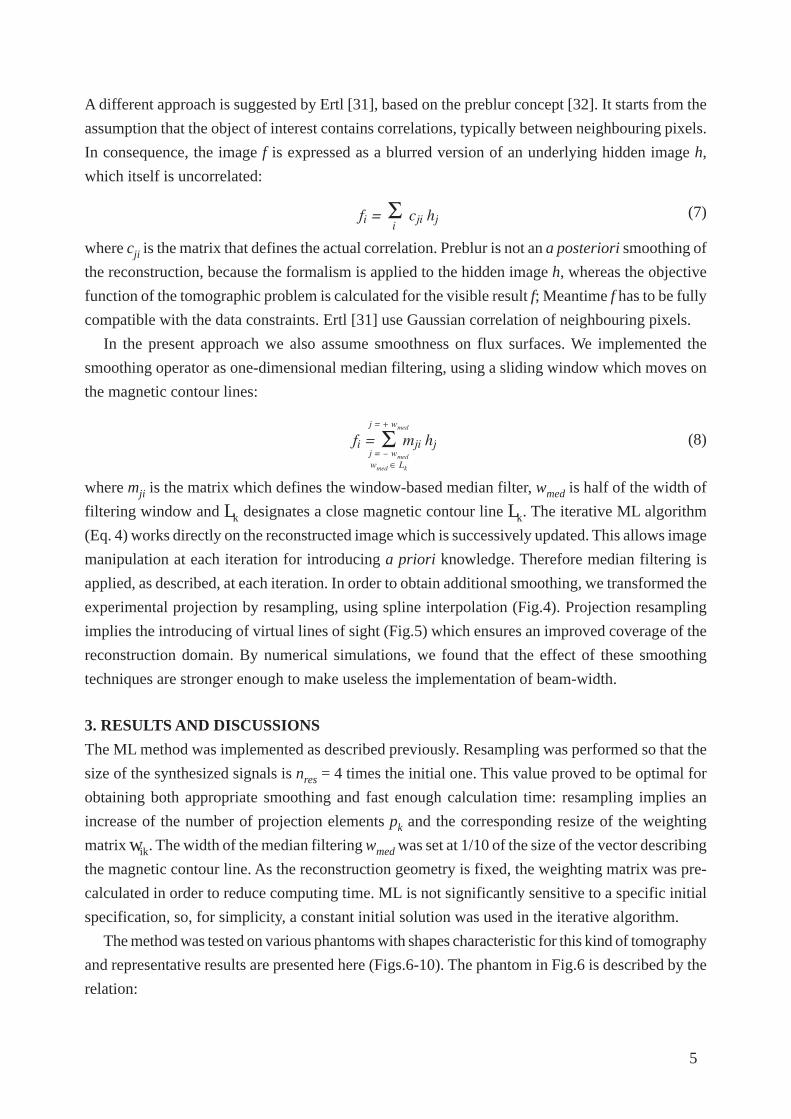
A different approach is suggested by Ertl [31], based on the preblur concept [32]. It starts from the

assumption that the object of interest contains correlations, typically between neighbouring pixels.

In consequence, the image f is expressed as a blurred version of an underlying hidden image h,

which itself is uncorrelated:

(7)

where cji is the matrix that defines the actual correlation. Preblur is not an a posteriori smoothing of

the reconstruction, because the formalism is applied to the hidden image h, whereas the objective

function of the tomographic problem is calculated for the visible result f; Meantime f has to be fully

compatible with the data constraints. Ertl [31] use Gaussian correlation of neighbouring pixels.

In the present approach we also assume smoothness on flux surfaces. We implemented the

smoothing operator as one-dimensional median filtering, using a sliding window which moves on

the magnetic contour lines:

(8)

where mji is the matrix which defines the window-based median filter, wmed is half of the width of

filtering window and kL designates a close magnetic contour line kL . The iterative ML algorithm

(Eq. 4) works directly on the reconstructed image which is successively updated. This allows image

manipulation at each iteration for introducing a priori knowledge. Therefore median filtering is

applied, as described, at each iteration. In order to obtain additional smoothing, we transformed the

experimental projection by resampling, using spline interpolation (Fig.4). Projection resampling

implies the introducing of virtual lines of sight (Fig.5) which ensures an improved coverage of the

reconstruction domain. By numerical simulations, we found that the effect of these smoothing

techniques are stronger enough to make useless the implementation of beam-width.

3. RESULTS AND DISCUSSIONS

The ML method was implemented as described previously. Resampling was performed so that the

size of the synthesized signals is nres = 4 times the initial one. This value proved to be optimal for

obtaining both appropriate smoothing and fast enough calculation time: resampling implies an

increase of the number of projection elements pk and the corresponding resize of the weighting

matrix ikw . The width of the median filtering wmed was set at 1/10 of the size of the vector describing

the magnetic contour line. As the reconstruction geometry is fixed, the weighting matrix was pre-

calculated in order to reduce computing time. ML is not significantly sensitive to a specific initial

specification, so, for simplicity, a constant initial solution was used in the iterative algorithm.

The method was tested on various phantoms with shapes characteristic for this kind of tomography

and representative results are presented here (Figs.6-10). The phantom in Fig.6 is described by the

relation:

fi = cji hjΣi

j = + wmed

j = - wmedwmed ∈ Lk

fi = mji hjΣ

6

(9)

where Npx is the number of pixels on the horizontal dimension of the reconstruction grid. Phantoms

in Figs. 7-8 were derived from the same circular symmetrical shape, by cutting half of the shape.

Virtual magnetic contour lines were simulated by circles placed concentrically on the

reconstruction grid. For the phantom in Fig. 9 the half-hollow shape from Fig.7 was distorted to

a elliptical symmetrical one (the vertical semi-axis is twice the horizontal one) and a centred

Gaussian A•exp - -x2

2πσ2 y2

2πσ2 yx

was superimposed (σx = 0.8 and σx = 1.6 and A = 0.18.Virtual

magnetic contour lines were simulated by concentric ellipses for which the ratio between the vertical

semi-axis and the horizontal one is equal to 2.

Good reconstructions are obtained for the “hollow” and “banana” phantoms (Figs.6-7). A more

difficult case is the reconstruction of the “banana” phantom, rotated by 180 degrees about the

vertical axis (Fig. 8). The diverging chords fan spread wider in this region and this results in a

reduced information density leading to a shadow effect. There are more possibilities in this region

to distribute each detector signal among different cells than in the region close to the detectors and

this may result in reduced spatial resolution. However, the decline in reliability with increasing

distance from the detector proved to be a tolerable effect. The shape of the “banana” is reconstructed

without global distortions. A blurring effect is superimposed on the image, however this does not

alter significantly the spatial resolution. We appreciate that this is also the inherent effect of smoothing

which is, on the other hand, essential for obtaining correct reconstructions. The spatial resolution of

the method is sufficient to resolve the complex shapes like “banana” plus peak (Fig.9).

The method was applied for the analysis of experimental data recorded at JET and significant

results are reported (Figs.10-13). In order to evaluate the performances of the ML method a

comparison with the results provided by the ICOM method [33] was performed. Similar

reconstruction of a “peak” phantom (most frequent distribution shape) is obtained by both methods

(Fig.10). This is the reconstructions of the DT-neutron emissivity profile in the experiment with the

T-puff in the deuterium plasma at 22.5s during the D neutral beam injection. In such experiments,

tritium is injected in ‘trace’ amount (typically nI / (nT + nD) <3% and the temporal evolution of the

tritium spatial distribution can be detected by observation of the 14MeV neutron emission, allowing

non-perturbative transients experiments. The neutron profile is a typical one for plasma with tritium

which has penetrated to the plasma core in full. The reconstruction of a “banana” distribution is

presented in Fig. 11. In this case DT-neutron emission was measured in the ohmic deuterium discharge

during the off-axis injection of the T neutral beam. Comparable reconstructions are obtained by

both methods. In comparison with ICOM, the ML reconstruction is affected by a slightly vertical

x2 + y2 , for

, for

ph(r) =<

2

Npx

Npx2

Npx

3/2x2 + y2

1/2

< <x2 + y21/2

1 - x2 + y21/2

7

asymmetry. The reconstruction of a combined “peak” plus “banana” distribution is illustrated in

Fig.12. This profile was recorded just after the T-puff in the same discharge as it has been presented

in the Fig.10, and tritons partly penetrated to the plasma core from the periphery. Thinner shapes

are obtained in case of ML method. We appreciate that this difference is due to the difference in the

definition of the smoothing: ICOM uses smoothing in both poloidal and radial direction

(anisotropically) while ML implements smoothing only along magnetic contour lines.

Besides spatial information, tomography is able to provide also information about the temporal

evolution of the neutron emissivity. The capability of the ML method to reveal this kind of information

is illustrated in Fig.13, where six reconstructions are taken in the temporal interval 20.87-21.32s.

They show the temporal evolution of the D-T 14MeV neutron emissivity in a trace tritium experiment.

The tomographic reconstruction demonstrates a relaxation of the high density plasma, which is

heated by D neutral beams after the T-puff at 20.5s. An evolution of the tritium penetration from the

edge toward the core can be clearly seen.

MATLAB was used as a suitable environment for developing and testing the method. In this

implementation the time needed for a reconstruction is lower than 3.5 minutes since 15-20 iterations

are typically enough to reach the maximum value of the correlation coefficient (Eq. 5). This is two

time faster than a single run of ICOM, which needs multiple runs for data preparation. As the

iterative algorithm (Eq. 4) can not be formulated in a matricial form (most suitable for MATLAB),

we expect to obtain a significant improvement of the calculation time in a further optimized

implementation. The computation speed, combined with accurate reconstruction represents an

advantage of the ML method which will qualify it as an appropriate method for inter-shot analysis.

CONCLUSION

In conclusion we appreciate that the ML reconstruction method provides good reconstructions in

terms of shapes and resolution. The smoothing techniques, introduced in order to compensate for

the lack of experimental information, induce a blurring effect but the correct reconstructions are

still practicable. The strategy used for smoothing implementation allows fast reconstructions. The

possibility of further optimization qualifies ML as a candidate for inter-shot analysis.

REFERENCES

[1] J.M. Adams, O.N. Jarvis, G.J. Sadler, D.B. Syme, N. Watkins, Nucl.Instrum.Methods A, 329

(1993) 277 290.

[2] O.N. Jarvis, J. M. Adams, F.B. Marcus, G.J. Sadler, Fusion Eng.Design, 34-35 (1997) 59 66.

[3] G. Bonheure, M. Angelone, R. Barnsley, L. Bertalot, S. Conroy, G. Ericsson, B. Esposito, J.

Kaellne, M. Loughlin, A. Murari, J. Mlynar, M. Pillon, S. Popovichev, B. Syme, M. Tardocchi,

M. Tsalas, Workshop on Fast Neutron Detection and Applications, Proc. of Science FNDA,

S. 091, 2006.

[4] M.J. Loughlin, N. Watkins, J.M. Adams, N. Basse, N.P. Hawkes, O.N. Jarvis, G. Matthews,

8

F.B. Marcus, M. O’Mullane, G. Sadler, J.D. Strachan, P. van Belle, K-D. Zastrow, Review of

Scientific Instruments 70 (1999) 1123 1125.

[5] R.S. Granetz, P. Smeulders, Nuclear fusion, 28 (1988) 457 476.

[6] F.B. Marcus, J.M. Adams, B. Balet, D.S. Bond, S.W. Conroy, P.J.A. Howarth, O.N. Jarvis,

M.J. Loughlin, G.J. Sadler, P. Smeulders, N. Watkins, Nuclear Fusion, 33 (1993) 1325 1344.

[7] L.C. Ingesson, B. Alper, H. Chen, A.W. Edwards, G.C. Fehmers, J.C. Fuchs, R. Giannella,

R.D. Gill, L. Lauro-Taroni, M. Romanelli, Nucl. Fusion 38 (1998) 1675.

[8] L.C. Ingesson,†H. Chen,†P. Helander,†M.J. Mantsinen, Plasma Physics and Controlled Fusion,

42 (2000) 161 180.

[9] M.J. Mantsinen, L.C. Ingesson, T. Johnson, V.G. Kiptily, M.-L. Mayoral, S. E. Sharapov, B.

Alper, L. Bertalot, Phys. Rev. Lett. 89 (2002) 115004-1-4.

[10] V.G. Kiptily, F.E. Cecil, O.N. Jarvis, M.J. Mantsinen, S.E. Sharapov, L. Bertalot, S. Conroy,

L.C. Ingesson, T. Johnson, K.D. Lawson, S. Popovichev, Nucl. Fusion 42 (2002) 999 1007.

[11] V.G. Kiptily, J.M. Adams, L. Bertalot, A. Murari, S.E. Sharapov, V. Yavorskij, B. Alper, R.

Barnsley, P. de Vries, C. Gowers, L.-G. Eriksson, P.J. Lomas, M.J. Mantsinen, A. Meigs, J.-

M. Noterdaeme, F.P. Orsitto, Nucl. Fusion 45 (2005) L21–L25.

[12] D. Stork, Yu. Baranov, P. Belo, L. Bertalot, D. Borba, J.H. Brzozowski, C.D. Challis, D.

Ciric, S. Conroy, M. de Baar, P. de Vries, P. Dumortier, L. Garzotti, N.C. Hawkes, T.C. Hender,

E. Joffrin T.T.C. Jones, V. Kiptily, P. Lamalle, J. Mailloux, M. Mantsinen, D.C. McDonald,

M.F.F. Nave, R. Neu, M. O’Mullane, J. Ongena, R.J. Pearce, S. Popovichev, S.E. Sharapov,

M. Stamp, J. Stober, E. Surrey, M. Valovic, I. Voitsekhovitch, H. Weisen, A.D. Whiteford, L.

Worth, V. Yavorskij, K.-D. Zastrow, Nucl. Fusion 45 (2005) S181–S194.

[13] N.C. Hawkes, V.A. Yavorskij, J.M. Adams, Yu F. Baranov, L. Bertalot, C.D. Challis, S. Conroy,

V. Goloborod’ko, V. Kiptily, S. Popovichev, K. Schoepf, S.E. Sharapov, D. Stork, E. Surrey,

Plasma Phys. Control. Fusion 47 (2005) 1475 1493.

[14] K.D. Zastrow, J.M. Adams, Yu Baranov, P. Belo, L. Bertalot, J.H. Brzozowski, C.D. Challis,

S. Conroy, M. de Baar, P. de Vries, P. Dumortier, J. Ferreira, L. Garzotti, T.C. Hender, E.

Joffrin, V. Kiptily, J. Mailloux, D.C. McDonald, R. Neu, M. O’Mullane, M.F.F. Nave, J.

Ongena, S. Popovichev, M. Stamp, J. Stober, D. Stork, I. Voitsekhovitch, M. Valovic, H.

Weisen, A.D. Whiteford, A. Zabolotsky, Plasma Phys. Control. Fusion 46 (2004) B255 B265.

[15] P.U. Lamalle, M.J. Mantsinen, J.-M. Noterdaeme, B. Alper, P. Beaumont, L. Bertalot, T.

Blackman, Vl.V. Bobkov, G. Bonheure, J. Brzozowski, C. Castaldo, S. Conroy, M. de Baar,

E. de la Luna, P. de Vries, F. Durodié, G. Ericsson, L.-G. Eriksson, C. Gowers, R. Felton, J.

Heikkinen, T. Hellsten, V. Kiptily, K. Lawson, M. LaxÂback, E. Lerche, P. Lomas, A.

Lyssoivan, M.-L. Mayoral, F. Meo, M. Mironov, I. Monakhov, I. Nunes, G. Piazza, S.

Popovichev, A. Salmi, M.I.K. Santala, S. Sharapov, T. Tala, M. Tardocchi, D. Van Eester, B.

Weyssow, Nucl. Fusion 46 (2006) 391 400.

[16] M Anton, H Weisen, M J Dutch, W von der Linden, F Buhlmann, R Chavan, B Marletaz, P

9

Marmillod, P Paris, Plasma Phys. Control. Fusion 38 (1996) 1849 1878.

[17] J. Mlynar, S. Coda, A. Degeling, B.P. Duval, F. Hofmann, T. Goodman, J.B. Lister, X. Llobet,

H. Weisen, Plasma phys. control. Fusion 45 (2003) 169 180.

[18] G. Bonheure, S. Popovichev, L. Bertalot, A. Murari, S. Conroy, J. Mlynar, I. Voitsekhovitch,

Nucl. Fusion 46 (2006) 725–740.

[19] G. Bonheure, J. Mlynar, L. Bertalot, S. Conroy, A. Murari, S. Popovichev, L. Zabeo, 32nd

EPS Conference on Plasma Phys. Tarragona, 27 June - 1 July 2005 ECA Vol.29C, P-1.083

(2005)

[20] T. Craciunescu, C. Niculae, Gh. Mateescu, C. Turcanu, J. Nucl. Mater. 224 (1995) 199 206

[21] I. Tiseanu, T. Craciunescu, 122 (1996) 384-394.

[22] S.H. Manglos, R.J. Jaszczak, C.E. Floyd, Phys. Med. Biol., 34 (1989) 1947 1957.

[23] K. Lange, Proc. SPIE Conf. Digital Image Synthesis and Inverse Optics, San Diego, CA,

1990, vol. SPIE-1351, pp. 270.

[24] L.A. Shepp, Y. Vardi, IEEE Transactions on Medical Imaging, Vol. 1 (1982) 113 121.

[25] R. Castro, M. Coates, M. Gadhiok, R. King, R. Nowak, E. Rombokas, Y. Tsang, Tech. Rep.

TREE-0107, Rice University, Aug. 2001. http://citeseer.ist.psu.edu/coates01maximum.html.

[26] A. Lvovsky, Journal of Optics B: Quantum and Semiclassical Optics 6 (2004) S556 S559.

[27] J. Rehacek, Z. Hradil, M. Zawisky, U. Bonse, F. Dubus, Phys. Rev., A, 71 (2005) 023608.1

023608.6.

[28] J. Rehacek, Z. Hradil, E. Knill, A. I. Lvovsky, Physical Review A, 75 (2007) 042108.1

042108.4.

[29] M.C. Borras, R.S. Granetz, Plasma Phys. Control. Fusion 38 (1996) 289.

[30] J. C. Fuchs, K. F. Mast, A. Hermann, K. Lackner, Proceedings of the 21st EPS Conference on

Controlled Fusion and Plasma Physics, Montpellier, 27 June – 1 July 1994, Ed. JOFFRIN, E.,

et al., Europhysics Conference Abstracts Vol. 18B (EPS, 1994), Part III, pp. 1308.

[31] K. Ertl, W. von der Linden, V. Dose, A. Weller, Nuclear Fusion, 36 (1996) 1477 1488.

[32] J. Skilling, in: P.F. FougËre (Ed.), Maximum Entropy and Bayesian Methods, Kluwer

Academic Publishers, Dordrecht (1990) pp. 341 350.

[33] JET Task Force DT, Library of 14 MeV tomography reconstructions, http://users.jet.efda.org/

pages/dt-task-force/pages/TTE_AlphaSources_Kiptily/AlphaSources_Table.htm

10

Figure 1: Schematic view of the JET neutron emission profile monitor showing the lines of sight.

Figure 2: The reconstruction domain coverage (the weightmatrix represented as an image): in case of infinitely thinline of sights (left) and taking into account the beam

Figure 3: Beam width representation

JG07

.433

-1c

Vertical camera

Detector box

Detector box

Remotelyselectablecollimators

#19

#19

#10

#10

#1

#11

#11

#1

Horizontalcamera

JG07

.433

-3c

JG

07.4

33-2

c

11

Figure 4. Projection resampling exemplified.

2 4 6 8 10

2 4 6 8 10 12 14 16 18

12 14 16 18

Inte

rpol

ated

Exp

erim

enta

l

Horizontal Camera Vertical Camera

JG07

.433

-4c

JG07

.433

-5c

Figure 5: Reconstruction of the hollow phantom.

12

Figure 7: Reconstruction of the symmetrically reversed“banana” phantom.

Figure 8: Reconstruction of the “banana” plus peakphantom

Figure 9: Neutron emissivity reconstruction for Pulse No:61132 at 22.92 s: ICOM (left) and ML (right).

Figure 6: Reconstruction of the “banana” phantom.

JG

07.4

33-6

c JG

07.4

33-7

c

JG

07.4

33-8

c

JG

07.4

33-9

c

13

Figure 11. Neutron emissivity reconstruction for shot61132 at 2.67s: ICOM (left) and ML (right).

Figure 10: Neutron emissivity reconstruction for PulseNo: 61237 at 6.22 – 6.27s s: ICOM (left) and ML (right)

JG

07.4

33-1

0c

JG07

.433

-13c

Figure 12. Temporal evolution of the neutron emissivity for Pulse No: 61141 (from 20.87 s to 21.32s)

JG07

.433

-11c

JG

07.4

33-1

2c

14