MCB 5472

Phylogenetic reconstruction likelihood and posterior probability

Peter Gogarten Office: BSP 404phone: 860 486-4061, Email: gogarten@uconn.edu

phyml PHYML - A simple, fast, and accurate algorithm to estimate large phylogenies by maximum likelihood

An online interface is here ; there is a command line version that is described here (not as straight forward as in clustalw); a phylip like interface is automatically invoked, if you type “phyml” – the manual is here.

Phyml is installed on bbcxsrv1.

Do example on atp_all.phyNote data type, bootstrap option within program, models for ASRV (pinvar and gamma), by default the starting tree is calculated via neighbor joining.

phyml - comments

The old version of phyml, under some circumstances calculated the consensus tree wrong. One solution was to save all the individual trees and to also evaluate them with consense from the phylip package. Note: phyml allows longer names, but consense allows only 10 characters!

phyml is fast enough to analyze dataset with hundreds of sequences (in 1990, a maximum likelihood analyses with 12 sequences (no ASRV) took several days).

For moderately sized datasets you can estimate branch support through a bootstrap analysis (it still might run several hours, but compared to protml or PAUP, this is extremely fast).

The paper describing phyml is here, a brief interview with the authors is here

Copyright © 2007 by the Genetics Society of America

Zhang, J. et al. Genetics 1998;149:1615-1625

Figure 1. The probability density functions of gamma distributions

Copyright © 2007 by the Genetics Society of America

Zhang, J. et al. Genetics 1998;149:1615-1625

Figure 4. Distributions of the {alpha} values of 51 nuclear (solid histograms) and 13 mitochondrial (open histograms) genes

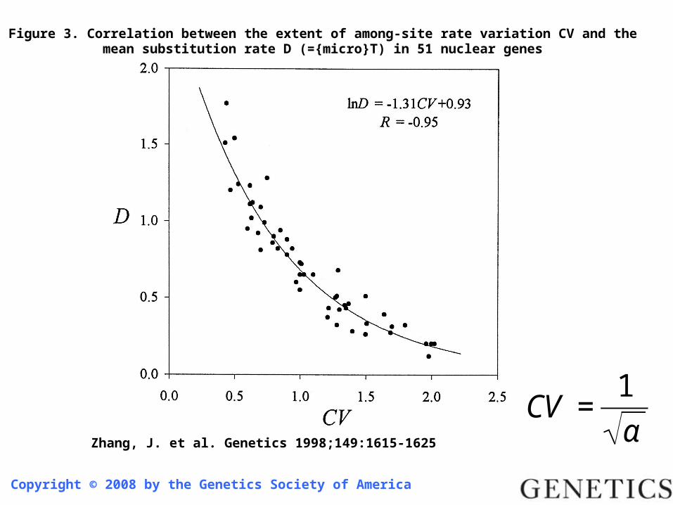
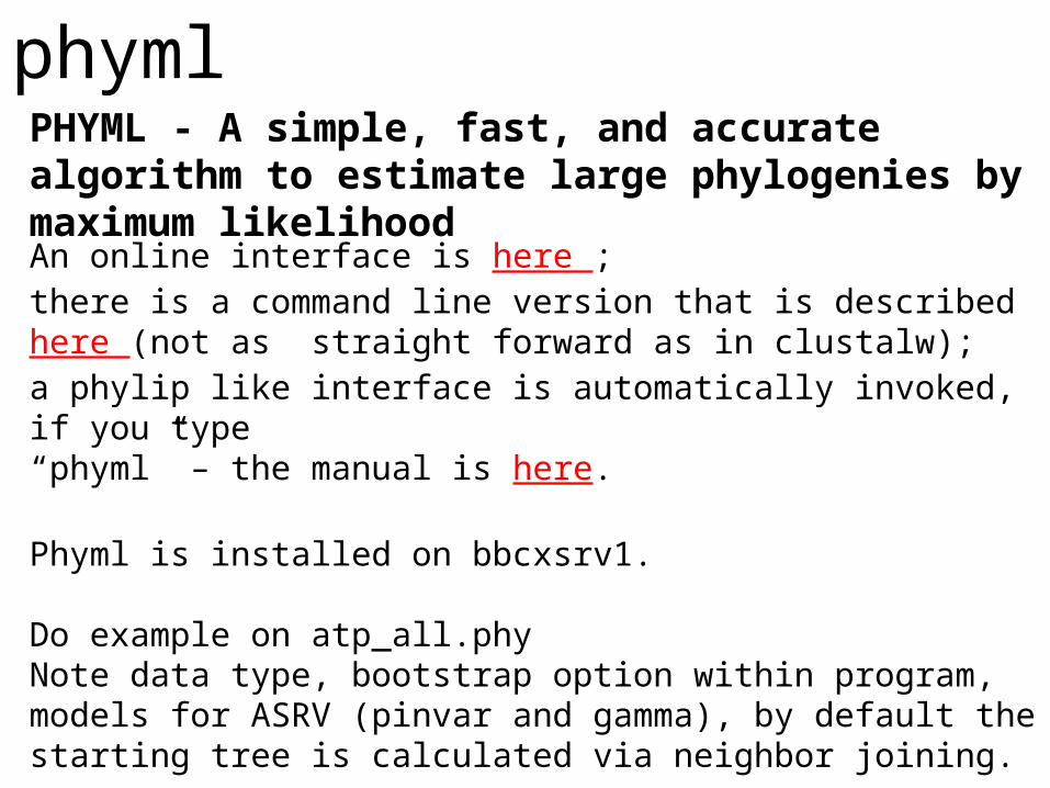
Copyright © 2008 by the Genetics Society of America

Zhang, J. et al. Genetics 1998;149:1615-1625

Figure 3. Correlation between the extent of among-site rate variation CV and the mean substitution rate D (={micro}T) in 51 nuclear genes

€

CV =1

α

TreePuzzle ne PUZZLE

TREE-PUZZLE is a very versatile maximum likelihood program that is particularly useful to analyze protein sequences. The program was developed by Korbian Strimmer and Arnd von Haseler (then at the Univ. of Munich) and is maintained by von Haseler, Heiko A. Schmidt, and Martin Vingron

(contacts see http://www.tree-puzzle.de/).

TREE-PUZZLE

allows fast and accurate estimation of ASRV (through estimating the shape parameter alpha) for both nucleotide and amino acid sequences,

It has a “fast” algorithm to calculate trees through quartet puzzling (calculating ml trees for quartets of species and building the multispecies tree from the quartets).

The program provides confidence numbers (puzzle support values), which tend to be smaller than bootstrap values (i.e. provide a more conservative estimate),

the program calculates branch lengths and likelihood for user defined trees, which is great if you want to compare different tree topologies, or different models using the maximum likelihood ratio test.

Branches which are not significantly supported are collapsed. TREE-PUZZLE runs on "all" platforms TREE-PUZZLE reads PHYLIP format, and communicates with the user

in a way similar to the PHYLIP programs.

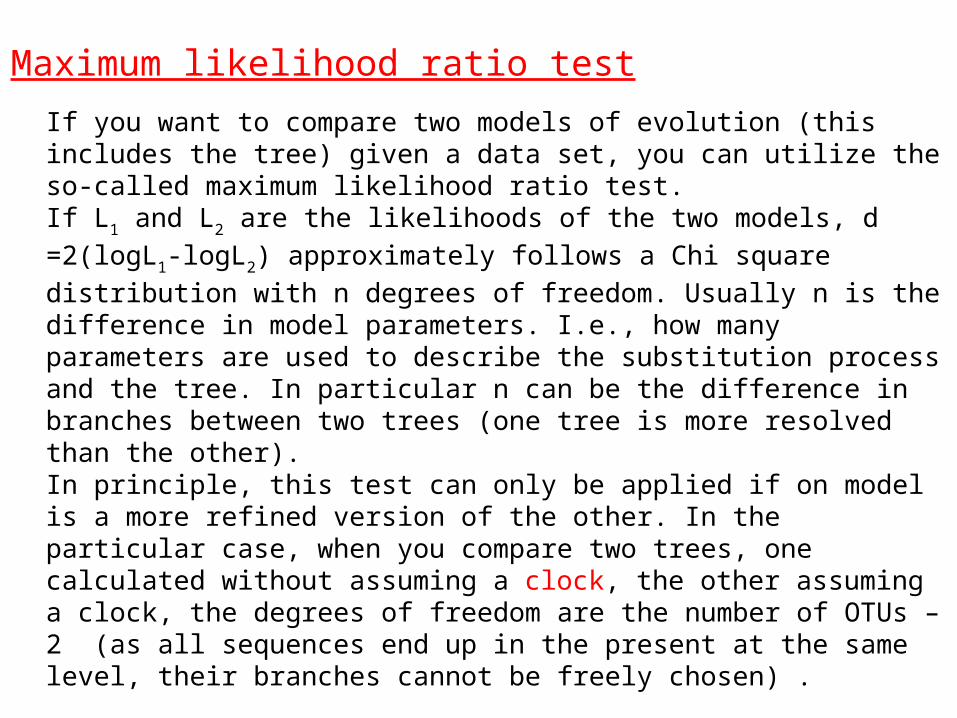
Maximum likelihood ratio test

If you want to compare two models of evolution (this includes the tree) given a data set, you can utilize the so-called maximum likelihood ratio test.  If L1 and L2 are the likelihoods of the two models, d =2(logL1-logL2)

approximately follows a Chi square distribution with n degrees of freedom. Usually n is the difference in model parameters. I.e., how many parameters are used to describe the substitution process and the tree. In particular n can be the difference in branches between two trees (one tree is more resolved than the other). In principle, this test can only be applied if on model is a more refined version of the other. In the particular case, when you compare two trees, one calculated without assuming a clock, the other assuming a clock, the degrees of freedom are the number of OTUs – 2 (as all sequences end up in the present at the same level, their branches cannot be freely chosen) .

To calculate the probability you can use the CHISQUARE calculator for windows available from Paul Lewis.

TREE-PUZZLE allows (cont) TREEPUZZLE calculates distance matrices using the ml

specified model. These can be used in FITCH or Neighbor.PUZZLEBOOT automates this approach to do bootstrap analyses –

WARNING: this is a distance matrix analyses!The official script for PUZZLEBOOT is here – you need to create a command file (puzzle.cmds), and puzzle needs to be envocable through the command puzzle.Your input file needs to be the renamed outfile from seqbootA slightly modified working version of puzzleboot_mod.sh is here, and here is an example for puzzle.cmds . Read the instructions before you run this!

Maximum likelihood mapping is an excellent way to assess the phylogenetic information contained in a dataset.

ML mapping can be used to calculate the support around one branch. @@@ Puzzle is cool, don't leave home without it! @@@

TREE-PUZZLE – PROBLEMS/DRAWBACKS

The more species you add the lower the support for individual branches. While this is true for all algorithms, in TREE-PUZZLE this can lead to completely unresolved trees with only a few handful of sequences.

Trees calculated via quartet puzzling are usually not completely resolved, and they do not correspond to the ML-tree:The determined multi-species tree is not the tree with the highest likelihood, rather it is the tree whose topology is supported through ml-quartets, and the lengths of the resolved branches is determined through maximum likelihood.

Elliot Sober’s Gremlins

?

??

Hypothesis: gremlins in the attic playing bowling

Likelihood = P(noise|gremlins in the attic)

P(gremlins in the attic|noise)

Observation: Loud noise in the attic

Bayes’ Theorem

Reverend Thomas Bayes (1702-1761)

Posterior Probability

represents the degree to which we believe a given model accurately describes the situationgiven the available data and all of our prior information I

Prior Probability

describes the degree to which we believe the model accurately describes realitybased on all of our prior information.

Likelihood

describes how well the model predicts the data

Normalizing constant

P(model|data, I) = P(model, I)P(data|model, I)

P(data,I)

Likelihood estimates do not take prior information into consideration:

e.g., if the result of three coin tosses is 3 times head, then the likelihood estimate for the frequency of having a head is 1 (3 out of 3 events) and the estimate for the frequency of having a head is zero.

€

P(A,B) = P(A,B)

€

P(A | B)∗P(B) = P(B | A) * P(A)

The probability that both events (A and B) occur

Both sides expressed as conditional probability

If A is the model and B is the data, then P(B|A) is the likelihood of model A P(A|B) is the posterior probability of the model given the data. P(A) is the considered the prior probability of the model. P(B) often is treated as a normalizing constant.

€

P(A | B) =P(B | A) * P(A)

P(B)

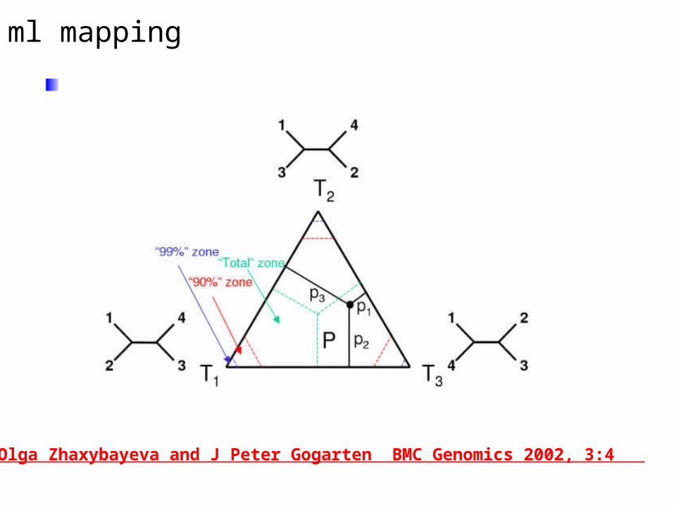
ml mapping

From: Olga Zhaxybayeva and J Peter Gogarten BMC Genomics 2002, 3:4 

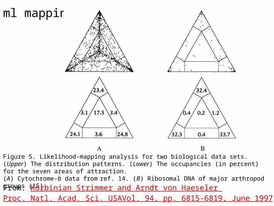
ml mapping

Figure 5. Likelihood-mapping analysis for two biological data sets. (Upper) The distribution patterns. (Lower) The occupancies (in percent) for the seven areas of attraction. (A) Cytochrome-b data from ref. 14. (B) Ribosomal DNA of major arthropod groups (15).

From: Korbinian Strimmer and Arndt von Haeseler Proc. Natl. Acad. Sci. USAVol. 94, pp. 6815-6819, June 1997

(a,b)-(c,d) /\ / \ / \ / 1 \ / \ / \ / \ / \ / \/ \ / 3 : 2 \ / : \ /__________________\ (a,d)-(b,c) (a,c)-(b,d)

Number of quartets in region 1: 68 (= 24.3%)Number of quartets in region 2: 21 (= 7.5%)Number of quartets in region 3: 191 (= 68.2%)

Occupancies of the seven areas 1, 2, 3, 4, 5, 6, 7:

(a,b)-(c,d) /\ / \ / 1 \ / \ / \ / /\ \ / 6 / \ 4 \ / / 7 \ \ / \ /______\ / \ / 3 : 5 : 2 \ /__________________\ (a,d)-(b,c) (a,c)-(b,d)

Number of quartets in region 1: 53 (= 18.9%) Number of quartets in region 2: 15 (= 5.4%) Number of quartets in region 3: 173 (= 61.8%) Number of quartets in region 4: 3 (= 1.1%) Number of quartets in region 5: 0 (= 0.0%) Number of quartets in region 6: 26 (= 9.3%) Number of quartets in region 7: 10 (= 3.6%)

Cluster a: 14 sequencesoutgroup (prokaryotes)

Cluster b: 20 sequencesother Eukaryotes

Cluster c: 1 sequencesPlasmodium

Cluster d: 1 sequences Giardia

Bayesian Posterior Probability Mapping with MrBayes (Huelsenbeck and Ronquist, 2001)

Alternative Approaches to Estimate Posterior Probabilities

Problem: Strimmer’s formula

Solution: Exploration of the tree space by sampling trees using a biased random walk

(Implemented in MrBayes program)

Trees with higher likelihoods will be sampled more often

piNi

Ntotal ,where Ni - number of sampled trees of topology i, i=1,2,3

Ntotal – total number of sampled trees (has to be large)

pi=Li

L1+L2+L3

only considers 3 trees (those that maximize the likelihood for the three topologies)

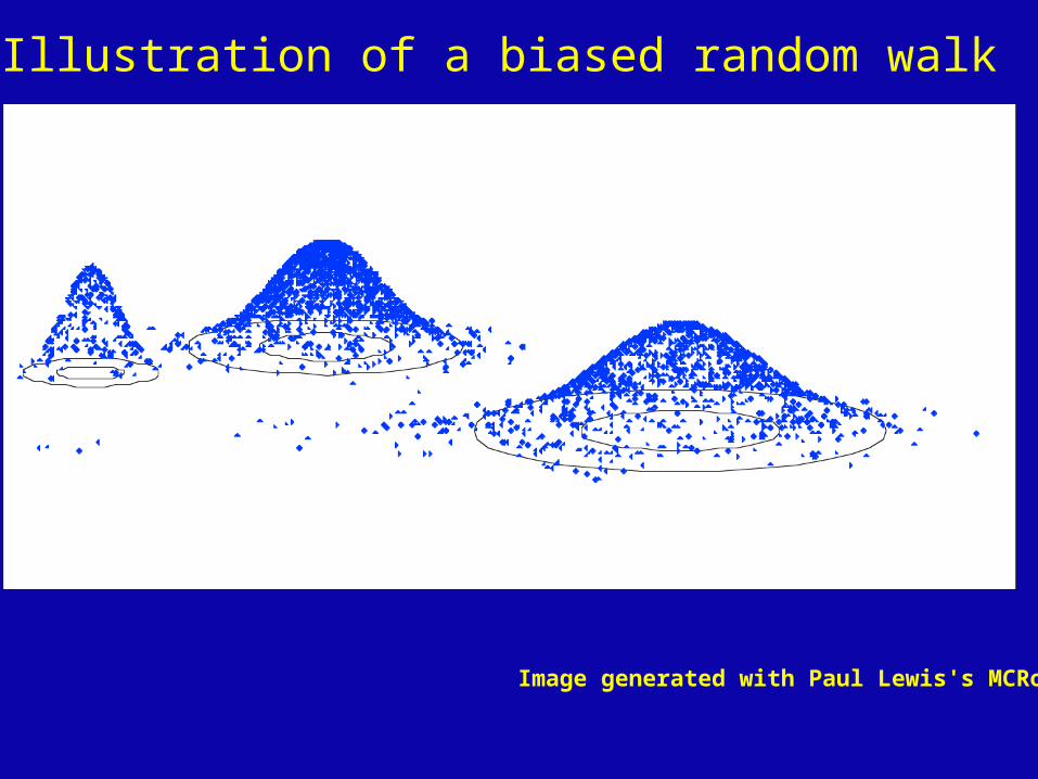
Illustration of a biased random walk

Image generated with Paul Lewis's MCRobot

Nexus files: This is the file format used by many popular programs like MacClade, Mesquite, ModelTest, MrBayes and PAUP*. Nexus file names often have a .nxs or .nex extension.

A formal description of the NEXUS format can be found in Maddison et al. (1997).

Conversion of an interleaved NEXUS file to a non-interleaved NEXUS file: execute the file in PAUP*, and export the file as non-interleaved NEXUS file. You can also type the commands:

export file=yourfile.nex format=nexus interleaved=no; clustalw saves and reads Nexus sequence and tree files (check on gap treatment and label as DNA or aa)

sample DNA file#nexus begin data;dimensions ntax=10 nchar=705;format datatype=dna interleave=yes gap=- missing=?;matrixCow ATGGCATATCCCATACAACTAGGATTCCAAGATGCAACATCACCAATCATAGAAGAACTACarp ATGGCACACCCAACGCAACTAGGTTTCAAGGACGCGGCCATACCCGTTATAGAGGAACTTChicken ATGGCCAACCACTCCCAACTAGGCTTTCAAGACGCCTCATCCCCCATCATAGAAGAGCTCHuman ATGGCACATGCAGCGCAAGTAGGTCTACAAGACGCTACTTCCCCTATCATAGAAGAGCTTLoach ATGGCACATCCCACACAATTAGGATTCCAAGACGCGGCCTCACCCGTAATAGAAGAACTTMouse ATGGCCTACCCATTCCAACTTGGTCTACAAGACGCCACATCCCCTATTATAGAAGAGCTARat ATGGCTTACCCATTTCAACTTGGCTTACAAGACGCTACATCACCTATCATAGAAGAACTTSeal ATGGCATACCCCCTACAAATAGGCCTACAAGATGCAACCTCTCCCATTATAGAGGAGTTAWhale ATGGCATATCCATTCCAACTAGGTTTCCAAGATGCAGCATCACCCATCATAGAAGAGCTCFrog ATGGCACACCCATCACAATTAGGTTTTCAAGACGCAGCCTCTCCAATTATAGAAGAATTA

Cow CTTCACTTTCATGACCACACGCTAATAATTGTCTTCTTAATTAGCTCATTAGTACTTTACCarp CTTCACTTCCACGACCACGCATTAATAATTGTGCTCCTAATTAGCACTTTAGTTTTATATChicken GTTGAATTCCACGACCACGCCCTGATAGTCGCACTAGCAATTTGCAGCTTAGTACTCTACHuman ATCACCTTTCATGATCACGCCCTCATAATCATTTTCCTTATCTGCTTCCTAGTCCTGTATLoach CTTCACTTCCATGACCATGCCCTAATAATTGTATTTTTGATTAGCGCCCTAGTACTTTATMouse ATAAATTTCCATGATCACACACTAATAATTGTTTTCCTAATTAGCTCCTTAGTCCTCTATRat ACAAACTTTCATGACCACACCCTAATAATTGTATTCCTCATCAGCTCCCTAGTACTTTATSeal CTACACTTCCATGACCACACATTAATAATTGTGTTCCTAATTAGCTCATTAGTACTCTACWhale CTACACTTTCACGATCATACACTAATAATCGTTTTTCTAATTAGCTCTTTAGTTCTCTACFrog CTTCACTTCCACGACCATACCCTCATAGCCGTTTTTCTTATTAGTACGCTAGTTCTTTAC

//Frog AACTGATCTTCATCAATACTA---GAAGCATCACTA------AGA;end;

sample aa file#NEXUS

Begin data;Dimensions ntax=10 nchar=234;Format datatype=protein gap=- interleave;MatrixCow MAYPMQLGFQDATSPIMEELLHFHDHTLMIVFLISSLVLYIISLMLTTKLTHTSTMDAQECarp MAHPTQLGFKDAAMPVMEELLHFHDHALMIVLLISTLVLYIITAMVSTKLTNKYILDSQEChicken MANHSQLGFQDASSPIMEELVEFHDHALMVALAICSLVLYLLTLMLMEKLS-SNTVDAQEHuman MAHAAQVGLQDATSPIMEELITFHDHALMIIFLICFLVLYALFLTLTTKLTNTNISDAQELoach MAHPTQLGFQDAASPVMEELLHFHDHALMIVFLISALVLYVIITTVSTKLTNMYILDSQEMouse MAYPFQLGLQDATSPIMEELMNFHDHTLMIVFLISSLVLYIISLMLTTKLTHTSTMDAQERat MAYPFQLGLQDATSPIMEELTNFHDHTLMIVFLISSLVLYIISLMLTTKLTHTSTMDAQESeal MAYPLQMGLQDATSPIMEELLHFHDHTLMIVFLISSLVLYIISLMLTTKLTHTSTMDAQEWhale MAYPFQLGFQDAASPIMEELLHFHDHTLMIVFLISSLVLYIITLMLTTKLTHTSTMDAQEFrog MAHPSQLGFQDAASPIMEELLHFHDHTLMAVFLISTLVLYIITIMMTTKLTNTNLMDAQE

//Loach QTAFIASRPGVFYGQCSEICGANHSFMPIVVEAVPLSHFENWSTLMLKDASLGSMouse QATVTSNRPGLFYGQCSEICGSNHSFMPIVLEMVPLKYFENWSASMI-------Rat QATVTSNRPGLFYGQCSEICGSNHSFMPIVLEMVPLKYFENWSASMI-------Seal QTTLMTMRPGLYYGQCSEICGSNHSFMPIVLELVPLSHFEKWSTSML-------Whale QTTLMSTRPGLFYGQCSEICGSNHSFMPIVLELVPLEVFEKWSVSML-------Frog QTSFIATRPGVFYGQCSEICGANHSFMPIVVEAVPLTDFENWSSSML-EASL--

;End;

Another example is here

More information on Nexus files and PAUP and

MrBayes commands are in the respective manuals: http://paup.csit.fsu.edu/, manual here, tutorial here

http://mrbayes.csit.fsu.edu/, manual here Wikki

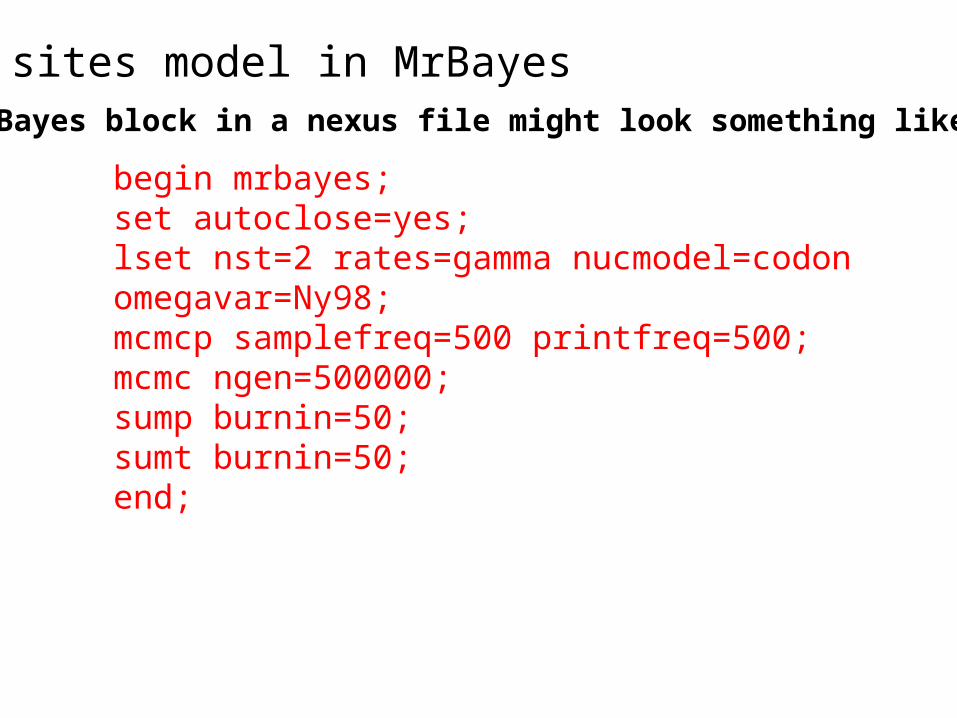
sites model in MrBayes

begin mrbayes; set autoclose=yes; lset nst=2 rates=gamma nucmodel=codon omegavar=Ny98; mcmcp samplefreq=500 printfreq=500; mcmc ngen=500000; sump burnin=50; sumt burnin=50; end;

The MrBayes block in a nexus file might look something like this:

Often in phylogenetic analysis the model and the prior information is very complex. For example, if you attempt to calculate a dated molecular phylogeny with a clock whose rate changes over the tree, and with some soft calibration points thrown in. To get an idea what the outcome of the model and constraints is without the data, run the chain without any data.

A: mapping of posterior probabilities according to Strimmer and von Haeseler

B: mapping of bootstrap support values

C: mapping of bootstrap support values from extended datasets

COMPARISON OF DIFFERENT SUPPORT

MEASURES

Zha

xyba

yeva

and

Gog

arte

n, B

MC

Gen

omic

s 20

03 4

: 37

bootstrap values from extended datasets

ml-mapping versus

More gene families group species according to environment than according to 16SrRNA phylogeny

In contrast, a themophilic archaeon has more genes grouping with the thermophilic bacteria

Sequence alignment:

Removing ambiguous positions:

Generation of pseudosamples:

Calculating and evaluating phylogenies:

Comparing phylogenies:

Comparing models:

Visualizing trees:

FITCHFITCH

TREE-PUZZLETREE-PUZZLE

ATV, njplot, or treeviewATV, njplot, or treeview

Maximum Likelihood Ratio TestMaximum Likelihood Ratio Test

SH-TEST in TREE-PUZZLESH-TEST in TREE-PUZZLE

NEIGHBORNEIGHBOR

PROTPARSPROTPARS PHYMLPHYMLPROTDISTPROTDIST

T-COFFEET-COFFEE

SEQBOOTSEQBOOT

FORBACKFORBACK

CLUSTALWCLUSTALW MUSCLEMUSCLE

CONSENSECONSENSE

Phylip programs can be combined in many different ways with one another and with programs that use the same file formats.

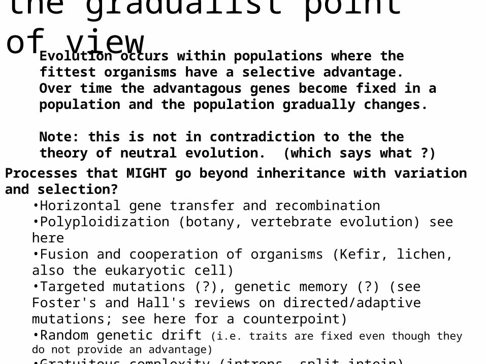
the gradualist point of viewEvolution occurs within populations where the fittest organisms have a selective advantage. Over time the advantagous genes become fixed in a population and the population gradually changes.

Note: this is not in contradiction to the the theory of neutral evolution. (which says what ?)

Processes that MIGHT go beyond inheritance with variation and selection? •Horizontal gene transfer and recombination •Polyploidization (botany, vertebrate evolution) see here •Fusion and cooperation of organisms (Kefir, lichen, also the eukaryotic cell) •Targeted mutations (?), genetic memory (?) (see Foster's and Hall's reviews on directed/adaptive mutations; see here for a counterpoint) •Random genetic drift (i.e. traits are fixed even though they do not provide an advantage)

•Gratuitous complexity (introns, split intein)•Selfish genes (who/what is the subject of evolution??) •Parasitism, altruism, Morons (Gene Transfer Agents)

Old exercises: Write a script that determines the number of elements in %ash. @keys = keys(%ash); #assigns keys to an array $number =@keys; # determines number of different keys (uses array in scalar context). print "$number \n";

Write a script that prints out a hash sorted on the keys in alphabetical order. @gi_names = sort(keys(%gi_hash)); # sorts key and assigns keys to an array foreach (@gi_names){ print "$_ occurred $gi_hash{$_} times\n"; }

Remove an entry in a hash (key and value): delete $gi_hash{$varaible_denoting_some_key};

Write a program that it uses hashes to calculates mono-, di-, tri-, and quartet-nucleotide frequencies in a genome. Carries over to next week

Assignments:

•Re-read chapter P16-P18 in the primer

•Given a multiple fasta sequence file*, write a script that for each sequence extract the gi number and the species name. and rewrites the file so that the annotation line starts with the gi number, followed by the species/strain name, followed by a space. (The gi number and the species name should not be separated by or contain any spaces – replace them by _. This is useful, because clustalw will recognize the number and name as handle for the sequence.)

•Work on your student project

•Assume that the annotation line follows the NCBI convention and begins with the > followed by the gi number, and ends with the species and strain designation given in []Example:>gi|229240723|ref|ZP_04365119.1| primary replicative DNA helicase; intein [Cellulomonas flavigena DSM 20109]

Example multiple sequence file is here.