The Lake Trout Rehabilitation Model:

Program Documentation

by

Carl J. Walters 1

Lawrence D. Jacobson

and

George R. Spangler*

Great Lakes Fishery Commission Special Publication No. 86-1

Citation: Walters, C. J., Jacobson, L. D., and G. R. Spangler. 1986. The laketrout rehabilitation model: program documentation. Great Lakes Fish.Corm. Spec. Pub. 86-l. 33 p,

GREAT LAKES FISHERY COMMISSION1451 Green Road

Ann Arbor, MI 48105USA

August, 1986

1 institute of Animal Resource Ecology 2 Department of Fisheries and WildlifeUniversity of British Columbia University of MinnesotaVancouver, B. C. V6T 1W5 200 Hodson HallCanada 1980 Folwell Avenue

St. Paul, MN 55108USA

The Lake Trout Rehabilitation Model:

Program Documentation

TABLE OF CONTENTS

Foreword ................................................................................................... 1

Overview .................................................................................................... 3

Functional Relationships ........................................................................ 3

References ................................................................................................ 9

Policy Analysis (Appendix A) .............................................................. 10

Instructions For Running The Model (Appendix B) .......................... 19

Flowchart (Appendix C) ....................................................................... 22

Listing of Computer Code (Appendix D) .......................................... .26

Modifications to the Original Model (Appendix E) . . . . . . . . . . . . . . . . . . . . . . . . . . . 33

The purpose of this report is to describe and document a computersimulation model known as “The Lake Trout Rehabilitation Model” written by

Carl Walters. The Lake Trout Rehabilitation Model has its roots in the work OfWalters et al. (1980) and in the Sea Lamprey International Symposium (SLIS)that was sponsored by the Great Lakes Fishery Commision and Convened in1979. Over time, and with the help Of numerous individuals, the Lake TroutRehabilitation Model evolved into its present form. Unlike the models describedby Koonce et al. (1982) and Spangler and Jacobson (1985), the Lake TroutRehabilitation Model was not written by a large team of experts during anadaptive management workshop.

The Lake Trout Rehabilitation Model simulates most aspects of lake troutpopulation biology, including factors that are thought to contribute to delayedrehabilitation of Great Lakes lake trout stocks: 1) mortality due to predation bysea lamprey, 2) fishing mortality, 3) reproductive incompetence of stocked fishand 4) time lags due to the relatively late age at maturity in lake trout. Themodel is realistic in that it includes the essential features of an age structuredpopulation and important biological characteristics of lake trout. It is importantto remember, however, that the model does not include some aspects of laketrout biology that may be crucial to the problem of lake trout rehabilitation,notably changes in growth of lake trout due to forage base limitations.Furthermore, the true functional relationships between some of the entities inthe model (e.g. mortality of lake trout and abundance of sea lamprey,abundance of sea lamprey and dollars spent for sea lamprey control) areunknown and are represented in the model by “best guesses”. For thesereasons results obtained using the Lake Trout Rehabilitation Model should beinterpreted qualitatively rather than quantitatively.

The Lake Trout Rehabilitation Model simulates rehabilitation of a troutstock from an initial condition of no fish. Rehabilitation is achieved throughcontrol of sea lamprey, lake trout stocking and limitations on fishing effort. Therate of rehabilitation depends on how much money is spent on lamprey control,the number of yearling lake trout stocked and the amount of fishing effort; thesepolicy variables are controlled by the person using the model. The model runsquickly (2 1/4 minutes to simulate 30 years) and plots the status of the simulatedtrout Stock and fishery on the screen at the end of every simulated year. Theuser can interrupt the simulation at any time in order to Chang8 the policyvariables. These features are important because they allow the user toexperiment with a variety of different policies for lake trout rehabilitation and tocontinuously monitor the effects of those pOliCi8S as the Simulation prOgr8SS8S.The potential for interactive use of the program and the degree of r8aliSm thatwas obtained make use of the Lake Trout Rehabilitation Model an interestingexercise.

The Lake Trout Rehabilitation Model is written in ApplesofP BASIC andwill run under Disk Operating System 3.3 (DOS 3.3) on any Apple llIH seri8Smicrocomputer with at least 64K of memory. The model can be obtained on a 51/4 inch floppy disk from the Great Lakes Fishery Commission or from George

1

Spangler. There are two versions of the program: “INTERACTIVETROUT. ORIGINAL” and “INTERACTIVE TROUT”. INTERACTIVETROUT. ORIGINAL is the original version written by Walters. INTERACTIVETROUT is a version that was modified by the junior authors. The modificationswere made to correct a minor bug and to enhance the readability of thecomputer code (see Appendix E). The original and modified VerSiOns are bothuseable and will give similar, though not identical, results.

Functional relationships used in the Lake Trout Rehabilitation Model aredescribed in the main body of this document. Policy analysis (using themodified version) is illustrated in Appendix A. Appendix B gives instructions forrunning the models. A flow chart and listing of the computer code are given forINTERACTIVE TROUT in Appendices C and D, respectively. Appendix Edescribes the differences between INTERACTIVE TROUT and INTERACTIVETROUT.ORIGINAL.

The Lake Trout Rehabilitation Model:

Program Documentation

OVERVIEW

The objective of the Lake Trout Rehabilitation Model is to simulatechanges in lake trout abundance using an age structured population model thatrealistically accounts for: 1) known time lags (between birth, stocking, maturityand recruitment to the fishery), 2) stocking policy, 3) differences in thereproductive capability of wild and stocked fish, 4) natural limits to recruitment(the stock-recruitment relationship and juvenile habitat capacity) and 5)mortality due to natural factors, lamprey predation and fishing. Not included inthe model are a number of more controversial relationships such as changes inthe forage base, changes in the abundance of alternate hosts for sea lampreyand changes in lake trout habitat due to pollution. The “slow dynamic” ofspawning habitat recolonization and adaptation of local stocks is notconsidered; instead, it is assumed that all major spawning shoals aresimultaneously recolonized as abundance of lake trout increases. The modelstarts from an initial condition of no fish. Abundance of lake trout increases asfish are stocked and as stocked fish begin to reproduce naturally. Thirty yearsof lake trout rehabilitation are simulated.

FUNCTIONAL RELATIONSHIPS

The following are detailed descriptions of the important functionalrelationships in the Lake Trout Rehabilitation Model. Values for constants andinitial values of variables are given in parentheses after the quantity is defined.

Age Structure

The number of fish age a in year t is related to the number of fish age a+1in year t+1 by:

VI

Where: Na,t = number of trout age a in year t,

M = natural mortality rate in the absence of sea lamprey (constant= 0.3),

Va = relative vulnerability to fishing for trout at age a (constant, see

Table 1 ),

3

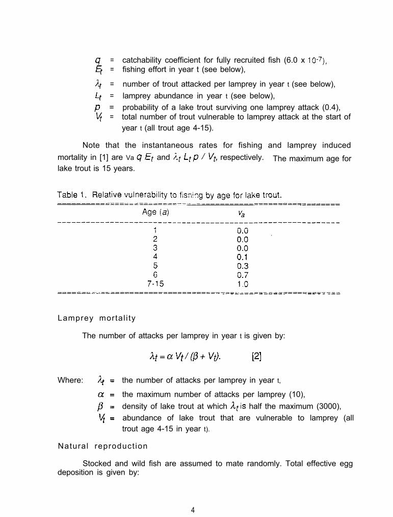
= catchability coefficient for fully recruited fish (6.0 x 1O-7),= fishing effort in year t (see below),

J-t = number of trout attacked per lamprey in year t (see below),

= lamprey abundance in year t (see below),

; = probability of a lake trout surviving one lamprey attack (0.4),= total number of trout vulnerable to lamprey attack at the start of

year t (all trout age 4-15).

Note that the instantaneous rates for fishing and lamprey induced

mortality in [1] are Va g Et and it Ltp / vt, respectively. The maximum age forlake trout is 15 years.

Lamprey mortal i ty

The number of attacks per lamprey in year t is given by:

Where: ;t= the number of attacks per lamprey in year t,

=

p”=

the maximum number of attacks per lamprey (10),

density of lake trout at which &is half the maximum (3000),

y= abundance of lake trout that are vulnerable to lamprey (alltrout age 4-15 in year t).

Natural reproduct ion

Stocked and wild fish are assumed to mate randomly. Total effective eggdeposition is given by:

4

Where: 4 = effective egg deposition in year t,

4 = the ratio of wild yearlings to total yearlings in year t,

s; := the ratio of wild fish to stocked fish in year t,

C2 = the average fecundity for fish age a,= proportion mature x proportion female X eggs per female

(Table 2),

tir,,= relative reproductive success for mating between two wild fish

(1.0),

aws = relative reproductive success for mating between a wild and astocked fish (0.75),

Qss = relative reproductive success for mating between two stocked

fish (0.5),m = the age of maturity (7),

i = the maximum age for lake trout (15).

All fish that result from spawning in the lake are assumed to be wild type atspawning time.

5

Limits to recruitment

The number of yearling recruits in year t+1 is given by:

Where: I\Jil,t+j = total number of yearlings in year t+l,

St+ 1 = number of yearlings stocked in year t +7 (2 million),

Ey = effective egg deposition in year t,

K = maximum number (carrying capacity) of wild yearlings (20million),

5-g = maximum survival rate from egg to yearling underuncrowded conditions (0.004).

The relationship between egg deposition and yearlings is illustrated in Figure 1.

6

Figure 1. Number of yearlings produced as a function of effective egg

deposition (assuming 2 million stocked yearlings).

0 20 40 60 80

EFFECTIVE EGG DEPOSITION (BILLIONS)

Fishing EffortFishing effort is a constant fraction of the vulnerable stock until a

maximum value is reached:

where E’, is the fishing effort in year t, Otis the number of fish vulnerable to

fishing in year t (Vt = ZVjNj,t) and E,ax is the maximum effort (1 million boat

days).

Lamprey control by expenditure of moneyThe relationship between lamprey abundance and dollars spent on

lamprey control (Figure 2) is given by:

Where Lt is the number of lamprey in year t and Dt is dollars spent on lampreycontrol in year t (6 million dollars). Expenditure of six million dollars gives50,000 lamprey, expenditure of zero dollars gives 200,000 lampreys.

7

Figure 2. Number of lamprey as a function of dollars spent on lamprey control.

8

REFERENCES

Eshenroder, R. L., J. F. Kitchell, C. H. Olver, T. P. Poe, and G. R. Spangler.1984. Overview, p. 44-50. In: R. L. Eshenroder, T. P. Poe, and C. H.Olver [ed.] Strategies for rehabilitation of lake trout in the Great Lakes:proceedings of a conference on lake trout research, August 1983. GreatLakes Fish. Comm. Tech. Rep. No. 40. 63 p.

Koonce, J. F. [ed.] 1982. A review of the adaptive management workshopaddressing salmonid/lamprey management in the Great Lakes. GreatLakes Fish. Comm. Spec. Publ. 82-2. 57 p.

Spangler, G. R., and L. D. Jacobson [ed.] 1985. A workshop concerning theapplication of integrated pest management (IPM) to sea lamprey controlin the Great Lakes. Great Lakes Fish. Comm. Spec. Publ. 85-2. 97 p.

Walters, C. J., G. Steer, and G. Spangler. 1980. Responses of lake trout(Salvelinus namaycush) to harvesting, stocking, and lamprey reduction.Can. J. Fish. Aquat. Sci. 37: 2133-2145.

9

APPENDIX A

POLICY Analysis

The following examples illustrate the way in which the Lake TroutRehabilitation Model can be used to investigate the effects Of stocking, harvestand sea lamprey control on rehabilitation of lake trout stocks. There are fourexamples. The first is a “baseline” scenario in which the number of fish stocked,maximum fishing effort and dollars spent on lamprey control are kept at theirinitial values (2 million fish, 6 million dollars and 1 million boat days,respectively) through the entire simulation. In the second scenario the amountof money spent for lamprey control is reduced to 2 million dollars (one-third thevalue used in the baseline case) in order to examine the effects of reduced sealamprey control on lake trout rehabilitation. Rehabilitation of lake trout in arefuge is depicted in the third example; fishing effort was zero boat days peryear through the entire simulation. In the fourth scenario the number of fishstocked is temporarily reduced in year 15 to zero. The effects of a one yearinterruption in the stocking program are illustrated. Most of these examples aretaken from the recommendations by Eshenroder et al. (1985) for large scalefield experiments. The axes in the following figures keep the same scale fromone scenario to the next in order to facilitate comparison of results from differentsimulations.

10

Figure Al. Simulation results for baseline scenario (2 million fish stockedannually, 6 million dollars spent annually for lamprey control, and 1 million boatdays per year as the maximum fishing effort). After 30 years of rehabilitation thenumber of 10 year old fish is negligible, wild fish constitute 50% of the maturestock and the annual catch is 400,000 fish.

11

Figure A2. Simulation results for scenario with reduced budget for lampreycontrol (2 million dollars annually for sea lamprey control, other controlvariables as in baseline scenario). Note that the rate of rehabilitation is muchreduced and that total catch in year 30 is about 1/4 the value obtained in thebaseline scenario.

13

Figure A3. Simulation results for scenario with no fishing effort. This is the onlyscenario that (gives an appreciable number of 10 year old fish and more than50% wild fish in the mature stock by year 30.

15

Figure A4. Simulation results for scenario with no fish stocked in year 15 (otherpolicy variables same as for baseline scenario). Note that the number ofyearlings in year 16 produced from natural reproduction in year 15 can beclearly seen in the upper right panel. By the end of the simulation, mostvariables are not much different from the levels obtained in the baselinescenario.

APPENDIX B

INSTRUCTIONS FOR RUNNING THE

LAKE TROUT REHABILITATION MODEL

Both versions of the Lake Trout Rehabilitation Model (INTERACTIVETROUT and INTERACTIVE TROUT.ORIGINAL) are written in ApplesoftM BASICand run under Disk Operating System 3.3 (DOS 3.3) on an Apple IIn* seriesmicrocomputer with at least 64K of memory. To run either model do thefollowing:

1) Insert the disk into the internal disk drive.

2) Turn the computer on. When the disk drive stops turning a greetingmessage is displayed.

3) Type “RUN” plus the name of the program plus a carriage return to load aprogram and run it (e.g. “RUN INTERACTIVE TROUT” followed by acarriage return). You can type “CATALOG” to see the names of the fileson the disk.

4) The program will ask you to press a key in order to start the simulation.

5) If you are using the or ig ina l vers ion ( i .e . INTERACTIVETROUT.ORIGINAL) then the simulation will commence immediately. Ifyou are using the modified version (i.e. INTERACTIVE TROUT) then the

program will give you the opportunity to change the policy variablesbefore the simulation begins. To change a policy variable type the new

value plus a carriage return in response to the appropriate prompt. Forexample, if you type 10000 plus a carriage return in response to theprompt “ANNUAL PLANTING (2000000):” then the number of yearlinglake trout planted annually will be changed from the old value (2000000)to the new value (10000). Typing a carriage return only in response to aquery will leave a value unchanged. A new value, once entered, is usedfor the remainder of the simulation or until it is changed again.

6) Once the simulation begins, you can interrupt the simulation in order tochange the policy variables at any time by pressing the space bar. Theprogram will stop within a few seconds and give you the opportunity tospecify new values for the policy variables. Follow the instructions in theinstruction above to change a policy variable.

7) The numbers of fish in ageclasses l-9 are printed (in thousands of fish)at the bottom of the screen at the end of every simulated year.

19

8) A number of variables are plotted on the screen at the end of eachsimulated year. If you have a Color monitor then the pIots for differentvariables will be in different colors. The variables are described in TableB1.

9) The model will simulate 30 years of lake trout rehabilitation. At the end ofthe simulation the program will prompt you to either quit or start a newsimulation. Press “Q” to quit or any other key will start a new simulation.If you press “Q” accidentally or change your mind about quitting then type“RUN” or “RUN” plus the version name followed by a carriage return.

20

Table B1. Description, plotting color and maximum value for the variablesplotted by the Lake Trout Rehabilitation Model.

Description Color Maximum Value

Panel 1 (upper left)number age 1 white 6 million fishnumber age 2 green 6 million fishnumber age 3 orange 6 million fish

Panel 2 (upper right)% wild yearlings% wild fish age >=5number yearlings stocked

white 100%green 100%orange 6 million fish

Panel 3 (lower left)sport efforttotal catchcatch of wild fish

whitegreenorange

10s boat days/year1 million fish1 million fish

Panel 4 (lower right)lamprey wounds per fish white 1 wound per fishnumber sea lamprey orange 300,000

21

APPENDIX C

FLOWCHART

The following is an informal flowchart that describes the order ofcomputations in the simulation program INTERACTIVE TROUT. Sections of thecomputer code that draw the graphic images on the screen are omitted from theflowchart for simplicity. The line numbers in the computer program at whichcomputations occur are indicated in parentheses.

22

START

DIMENSION ARRAYS (20-70),LOAD MACHINE LANGUAGE ROUTINE (80),

PRINT GREETING AND TITLE OF PROGRAM (90-110)

RESET DATA POINTER,INITIALIZE VARIABLES,

DRAW PLOTS AND LABELS ON SCREEN (120-130)

START SIMULATION (140-l 50)

YESHAS THE USER PRESSED A KEY

TO INTERRUPT THE SIMULATION?(160-170)

REPEAT FOR EACHCHANGE POLICY

TIME STEP UNTILVARIABLES

NOSIMULATION IS COMLETE

(920-960)

(FROM 860)

INITIALIZE VARIABLES FOR CURRENT TIME STEP(190-200)

PRINT ABUNDANCES FOR AGES 1-9 ON SCREEN (210-220)

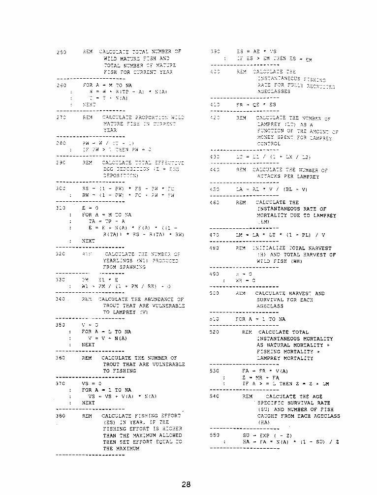
CALCULATE TOTAL NUMBER WILD MATURE FISH ANDTOTAL NUMBER OF MATURE FISH IN CURRENT YEAR

(230-240)

(NEXT PAGE)

CALCULATE PROPORTION WILD MATURE FISH IN CURRENT YEAR(250-260)

CALCULATE TOTAL EFFECTIVE EGG DEPOSITION (270-280)

CALCULATE NUMBER OF YEARLINGS PRODUCED FROM EGGS LAIDIN CURRENT YEAR (290.310)

CALCULATE TOTAL NUMBER OF YEARLINGS (NATURAL REPRODUCTION +STOCKING) AND THE PROPORTION WILD YEARLINGS FOR CURRENT YEAR

(320-330)

CALCULATE ABUNDANCE OF TROUT VULNERABLE TO LAMPREY (340-350)

CALCULATE THE NUMBER OF TROUT VULNERABLE TO FISHING (360-370)

CALCULATE FISHING EFFORT FOR CURRENT YEAR (380-390)

CALCULATE INSTANTANEOUS FISHING RATE FOR FULL RECRUITEDAGECLASSES (400-410)

CALCULATE THE NUMBER OF LAMPREY FROM DOLLARS SPENT ONLAMPREY CONTROL (420-430)

(NEXT PAGE)

APPENDIX D

LISTING of COMPUTER CODE

The following is a complete listing of the Lake Trout Rehabilitation Modelnamed INTERACTIVE TROUT. The dashed lines between lines of computercode are meant to improve readability; they are not part of the code.

26

APPENDIX E

MODIFICATIONS BY THE EDITORS To THE ORIGINAL MODEL

1) A comment was added to every line of code that had biologicalsignificance.

2) The code was renumbered (the first line in the new version isnumber 10, each line increments by 10).

3) The subscript on the vector F in line 240 of the original version(line 310 in the modified version) was changed from A-M to A. Thefecundity table in line 10030 of the original model was altered tocomplement the subscript change (lines 1210-1220 in themodified version). As a result of these changes the fecundity tableand egg deposition calculations are indexed by age. Themodifications do not affect numerical results.

4) The order of calculations in the original model was changed sothat the number of yearlings in year t is the sum of yearlingsproduced from spawning in year t-1 and yearlings stocked in yeart. The relevant line numbers are 250-260 in the original versionand 240 and 330 in the modified version.

GREAT LAKES FISHERY COMMISSION

SPECIAL PUBLICATIONS

79-l Illustrated field guide for the classification of sea lamprey attack marks on GreatLakes lake trout. 1979. E. L. King and T. A. Edsall. 41 p.

82-1 Recommendations for freshwater fisheries research and management from theStock Concept Symposium (STOCS). 1982. A. H. Berst and G. R. Spangler. 24 p.

82-2 A review of the adaptive management workshop addressing salmonid/lampreymanagement in the Great Lakes. 1982. Edited by J. F. Koonce, L. Greig,B. Henderson, D. Jester, K. Minns, and G. Spangler. 40 p.

82-3 Identification of larval fishes of the Great Lakes basin with emphasis on the LakeMichigan drainage. 1982. Edited by N. A. Auer. 744 p.

83-l Quota management of Lake Erie fisheries. 1983. Edited by J. F. Koonce,D. Jester, B. Henderson, R. Hatch, and M. Jones. 39 p.

83-2 A guide to integrated fish health management in the Great Lakes basin. 1983.Edited by F. P. Meyer, J. W. Warren, and T. G. Carey. 262 p.

84-l Recommendations for standardizing the reporting of sea lamprey marking data.1984. R. L. Eshenroder, and J. F. Koonce. 21 p.

84-2 Working papers developed at the August 1983 conference on lake trout research.1984. Edited by R. L. Eshenroder, T. P. Poe, and C. H. Olver.

84-3 Analysis of the response to the use of “Adaptive Environmental AssessmentMethodology*’ by the Great Lakes Fishery Commission. 1985. C. K. Minns, J. M.Cooley, and J. E. Forney. 21 p.

85-l Lake Erie fish community workshop (report of the April 4-5, 1979 meeting).1985. Edited by J. R. Paine and R. B. Kenyon. 58 p.

85-2 A workshop concerning the application of integrated pest management (IPM) tosea lamprey control in the Great Lakes. 1985. Edited by G. R. Spangler and L. D.Jacobson. 97 p.

85-3 Presented papers from the Council of Lake Committees plenary session on GreatLakes predator-prey issues, March 20, 1985. 1985. Edited by R. L. Eshenroder.134 p.

85-4 Great Lakes fish disease control policy and model program. 1985. Edited by J. G.Hnath. 24 p.

85-5 Great Lakes Law Enforcement/Fisheries Management Workshop (Report of the 21,22 September 1983 meeting). 1985. Edited by W. L. Hartman and M. A. Ross.26 p.

85-6 TFM vs. the sea lamprey: a generation later. 1985. 17 p.