ASTRONOMY & ASTROPHYSICS OCTOBER I 1999, PAGE 183

SUPPLEMENT SERIES

Astron. Astrophys. Suppl. Ser. 139, 183–197 (1999)

The IUE INES System: Improved data extraction procedures forIUE

P.M. Rodrıguez-Pascual1,?, R. Gonzalez-Riestra2,?, N. Schartel3,?,??, and W. Wamsteker4,??

1 Departamento de Fısica, Universidad Europea de Madrid, C/Tajo S/N, 28670 Villaviciosa de Odon, Spain2 LAEFF, P.O. Box 50727, 28080 Madrid, Spain3 ESA - XMM SOC, P.O. Box 50727, 28080 Madrid, Spain4 ESA - IUE Observatory, P.O. Box 50727, 28080 Madrid, Spain

Received March 1; accepted June 28, 1999

Abstract. We present the extraction and processing ofthe IUE Low Dispersion spectra within the framework ofthe ESA “IUE Newly Extracted Spectra” (INES) System.Weak points of SWET, the optimal extraction imple-mentation to produce the NEWSIPS output products(extracted spectra) are discussed, and the procedures im-plemented in INES to solve these problems are outlined.The more relevant modifications are: 1) the use of a newnoise model, 2) a more accurate representation of the spa-tial profile of the spectrum and 3) a more reliable deter-mination of the background. The INES extraction alsoincludes a correction for the contamination by solar lightin long wavelength spectra. Examples showing the im-provements obtained in INES with respect to SWET aredescribed. Finally, the linearity and repeatability charac-teristics of INES data are evaluated and the validity ofthe errors provided in the extraction is discussed.

Key words: methods: data analysis — space vehicles —techniques: image processing — ultraviolet: general

1. Introduction

The International Ultraviolet Explorer (IUE) collectedmore than 104000 spectra of all types of astronomical ob-jects during its more than 18 years of operations. TheIUE Project considered it desirable to make available tothe astronomical community a “Final Archive” holdingall the IUE data processed in an uniform way and withimproved reduction techniques and calibrations. For this

Send offprint requests to: P.M. Rodrıguez-Pascual? Previously: ESA - IUE Observatory.?? Affiliated to the Astrophysics Division, SSD, ESTEC.

Correspondence to: p miguel.rodriguez@fis.cie.uem.es

purpose a new processing system (NEWSIPS) was devel-oped and the full IUE archive was re-processed with anewly derived linearization and wavelength scale. Also anadapted optimal extraction scheme (Horne 1986), SWET,was used to derive the low resolution absolutely calibratedoutput spectra. A full description of the NEWSIPS sys-tem is given in Nichols & Linsky (1996) and in Nichols(1998). Technical details can be found in the NEWSIPSManual (Garhart et al. 1997).

One of the main goals of the system is to obtainthe maximum signal-to-noise ratio in the final data.For this purpose the geometric and photometric cor-rections are performed through a new approach, basedon cross-correlation techniques to align science andIntensity Transfer Functions (ITF) images (Linde &Dravins 1990). The application of this new approachreduces substantially the fixed pattern noise, and leadsto improvements in the signal-to-noise ratio between 50and 100% in low dispersion spectra and between 50 and200% in high resolution data (Nichols 1998).

The intrinsic non-linearity of the detectors (SECVIDICON cameras) makes the photometric correctionone of the most critical tasks in the processing ofIUE data. The correction is performed through theIntensity Transfer Functions (ITFs), which are derivedfrom series of graded lamp exposures. These functionstransform the raw Data Numbers (DN) of each pixelin the Raw Image into linearized Flux Numbers (FN)in the Photometrically Corrected Image. Specificallyfor the Final Archive, a new set of ITFs images wereobtained for the three cameras under well controlledspacecraft conditions and through improved algorithms.However, the final extracted spectra still show someresidual non-linearities, most likely due to the breakdownat the extreme ITF levels of the assumption that oversmall differential flux ranges the relation between FNsand DNs can be approximated by a linear interpolation.

184 P.M. Rodrıguez-Pascual et al.: INES low resolution data

Further modifications implemented in NEWSIPS in-clude the improvement in the wavelength calibration, therevision of the flux scale, the derivation of noise modelsand the optimal extraction of spectra (only for low reso-lution). The existence of noise models has allowed to esti-mate the errors on IUE fluxes for the first time. A specialeffort has also been made to ensure the correctness of allthe information referring to the specific observation at-tached to the data.

The quality control procedures applied by the IUEProject have shown that the NEWSIPS reprocessed spec-tra are superior to the IUESIPS spectra in all cases(Nichols 1998). For the high resolution spectra the newmethods to estimate the image background (Smith 1998)and the ripple correction algorithm (Cassatella et al. 1998)result in a much higher quality high resolution spectra forthis data. However, it was found that the low resolutiondata extraction still contained some serious shortcomingswhich would affect significantly the usefulness of the ex-tracted spectra. (Talavera et al. 1992; Nichols 1998). Mostof these shortcomings and drawbacks in the IUEFA prod-ucts were related to the method for the final extractionof the 1-D spectra (SWET) from the bi-dimensional, spa-tially resolved, rotated images (SILO1 files).

Within the framework of the ESA IUE DataDistribution System, it was decided to correct all thelow dispersion spectra through the application of newextraction algorithms that significantly improve thequality and reliability in the final data products. Acompletely different philosophy is behind these newalgorithms. The model-dependent strategy followed inSWET is abandoned, with the aim of retaining as muchinformation as possible concerning the data. We antici-pate that the results of both techniques are essentiallyidentical, when the model parameters used by SWET arewell suited, namely, for well exposed continuum sources.The method chosen has assured that the improvementsachieved with the NEWSIPS geometric and photometriccorrections are preserved since the new algorithms workon the SILO files. In this paper we describe the mainfeatures of the INES extraction procedures: backgroundand spatial profile determination, quality flags handling,solar contamination removal, homogenization of thewavelength scale (Sect. 2).

In Sect. 3 the repeatability, errors reliability and lin-earity of INES low dispersion data are evaluated. Finally,the major improvements achieved by INES are summa-rized in Sect. 4.

1 The photometrically and geometrically corrected image isrotated so that the dispersion direction is along the X axis.

2. Optimal extraction of IUE Low dispersion spectra

Optimal extraction techniques for bidimensional detectorswere originally developed for CCD chips (Horne 1986).The basic equations of the method are:

FN(λ) =

∑x [FN(x, λ)−B(x, λ)] p(x,λ)

σ(x,λ)2∑xp(x,λ)2

σ(x,λ)2

(1)

1∆FN(λ)2

=∑x

p(x, λ)2

σ(x, λ)2(2)

where the variables are:

– x: coordinate in the cross-dispersion (spatial) direc-tion,

– λ: coordinate in the spectral direction,– FN(x, λ): FN value at pixel (x, λ),– B(x, λ): background at pixel (x, λ),– σ(x, λ): noise at pixel (x, λ),– p(x, λ): extraction profile at pixel (x, λ),– FN(λ): total flux number (FN) at λ.

It must be noted that the IUE detectors are quite differentfrom CCDs, which are nearly linear detectors, with a verylarge dynamic range, formed by individual pixels, almostindependent on their neighbors. None of these character-istics are valid for the IUE SEC Vidicon cameras. Eachraw IUE image consist on a 768 × 768 array of 8-bit ele-ments, which are not physical pixels, but picture elementsdetermined by the stepping and size of the camera read-out beam. The focusing system of this beam introducesgeometric distortions. The dynamic range is small (0-255DN) and the response of the camera is non-uniform andhighly non-linear. Furthermore, the noise in these detec-tors deviates strongly from the poissonian photon noise ofCCDs.

Therefore, a direct application of the techniques usedfor CCDs is not appropriate. The application of Eq. (1)to IUE data requires a careful determination of the noisemodel, the background estimation, the extraction profileand the treatment of “bad” pixels. Furthermore, these de-terminations are model dependent and the best results areobtained only after fine tuning a number of parameters.In an interactive processing the choice of the best set ofparameters is made case by case. For automatic process-ing, these processing parameters are fixed and must bechosen so as to cover the largest number of possible cases.This approach unavoidably leads to the degradation of theperformance of the system.

In the following subsections, the main items enteringin the optimal extraction process are discussed, indicatingthe solutions adopted in SWET and identifying the prob-lems which have led to the different extraction schemeapplied in INES.

P.M. Rodrıguez-Pascual et al.: INES low resolution data 185

2.1. Noise models

The estimate of the noise in IUE data is essential at twostages of the extraction of the spectrum from the SILOimages. Firstly, the determination of the extraction pro-file requires an evaluation of the signal-to-noise ratio inorder to perform weighted fits to the data. Secondly, theerrors in individual pixels are propagated through the ex-traction procedure in order to assign errors to the finalextracted fluxes.

The characteristics of the noise in the IUE Raw imagesare strongly altered by the photometric linearization pro-cedure via the Intensity Transfer Function and by the spa-tial resampling required to derive the SILO image format.The approach followed to derive the noise model in SWET,as well as in INES, has been to model it empirically fromSILO science and lamp (UV-flood) images (Garhart et al.1997). However the final noise models in the INES proce-dure are different from that used in SWET in two points:the extrapolation to high FN values and the handling ofvery low FN values. In the first case, the SWET noisemodel extrapolates a third order polynomials determinedfrom the fitting of lower FN ’s. These polynomials oftenhave a negative derivative for high FN values, leading tounrealistic estimates of the noise as shown in Fig. 1. Atthe low end of the FN range, SWET noise models also usehigh order polynomials which introduces strong boundaryeffects. It is especially remarkable that SWET assigns anerror of 1 FN to negative FNs, which occurs becauseof statistical fluctuations around the adopted NULL ITFlevel.

Fig. 1. Example of the noise model for the wavelength 1612 A.Points represent the standard deviation σ(FN) as a function ofthe corresponding median flux numbers < FN >0. The crossesindicate data not considered for the modeling. The continuousline shows the noise model applied in INES consisting of a fit-ted polynomial and its linear extrapolation. The broken lineshows the SWET extrapolated polynomial for comparison

In the INES noise models, for every wavelength in-terval the standard deviation as a function of the FNis described by polynomials of different order for differ-ent FN ranges. For FN values below thirty, a first orderpolynomial was used in order to avoid boundary effects.In the FN range from thirty up to the point where stillenough data points are available (“breakpoint”) a higherorder polynomial was used (third degree for LWP, fourthfor SWP and LWR). The region of higher FN is linearlyextrapolated based on the third (fourth) order polynomialfit (Fig. 1). Therefore, for a given wavelength, λ the noise,σ(FN), is represented by:

σ(FN)|λ=const. =

B1 + C1 · FN for FN ≤ 30

4(SWP),3(LWP)∑i=0

Ai · FN i for 30 ≤ FN ≤ breakpoint

B2 + C2 · FN for FN > breakpoint.

The fitting of the third (fourth) order polynomial was it-erated five times, excluding data points for which σ(FN)was greater then two times the values fitted in the previ-ous iteration in order to exclude cosmic rays and similarfeatures.

The extrapolation to high FN values was based onthe fifty highest data points. The “breakpoint” was de-fined as the value with the largest positive derivative. Forthe LWP camera the “breakpoints” are found at valuesbetween 390 and 460 FN , depending on the wavelength.For SWP they are in the range 280 to 400 FN , and forLWR in the range 105 to 410. Therefore the extrapolationin the LWR camera covers a larger range of FNs.

The noise models were smoothed in the wavelengthdirection following a similar approach, i.e. different poly-nomials were used for different cameras and wavelengthranges.

Finally, the noise model was interpolated over a two di-mensional grid of 1025 FN values (from 0 to 1024) by 640pixels in the wavelength direction. In the cases in whichthe SILO file has negative FN values, the noise of thesepixels is taken as the value corresponding to FN = 0 forthat wavelength.

As expected, both noise models are indistinguishablefor most FN values and wavelengths. It is only in veryshort exposure time images and/or images with pixelsreaching FN values larger than the “break-points” de-fined above that different results are obtained. It shouldbe noticed that in the SWET method a single high FNpixel with an incorrectly extrapolated error may affect sig-nificantly the extraction profile determination because ofthe exceptional signal-to-noise ratio assigned to it.

186 P.M. Rodrıguez-Pascual et al.: INES low resolution data

2.2. Spectral extraction

According to Eq. (1), the three major items in the optimalextraction method are: the background, the spatial profileand the noise model. Their treatment in the INES extrac-tion procedure is described in following subsections. Inaddition, a subsection is devoted to describe the handlingof those pixels whose quality is non-optimal. The methodapplied to remove the solar contamination in LWP im-ages is also described in detail in a separate subsection.Finally, the method to homogenize the wavelength scalefor all long and short wavelength spectra, independentlyof observing epoch or ITF, is outlined.

2.2.1. Background determination

The background in IUE science images is a combinationof different sources: particle radiation, radioactive phos-phor decay in the detector, halation within the UV con-verter, background skylight, scattered light and readoutnoise. The first two depend on the instrument itself andon the radiation environment and vary slowly across thecamera faceplate, whereas the last three depend on thespectral flux distribution of the object observed and theirintegrated effect varies in a complicated way across theraw image.

The background is derived from two swathes seven pix-els wide in the spatial direction, symmetrically locatedwith respect to the center of the aperture.

Fig. 2. Example of background smoothing in INES (solid line).The dashed line represents the 6th degree polynomial fit usedin SWET

Along the dispersion direction, the method to estimatethe background has to remove the high frequency noise butpreserving the low frequency intrinsic variations. The twoapproaches generally followed in the past have been (a) toapply consecutively a median and a box filter (IUESIPS)or (b) to fit the background to a polynomial (SWET). Adirect smoothing is simple, robust and model independent,but sensitive to bright spots and outlying pixels. A poly-nomial fit is more efficient in removing such outliers, but

the degree of the polynomial must be too high to repro-duce the small scale variations. As a compromise providingacceptable solutions, we have adopted for INES an itera-tive method in which the background is median and boxfiltered (31 pixels wide), allowing for outlying pixels re-jection in each iteration. This method effectively reducesthe noise, preserves the intrinsic background variations inrelatively small scales and removes bright spots (Fig. 2).

Fig. 3. This figure shows an example where there are small, butsignificant, variations of the background in the spatial direc-tion. The dashed line is the average of the SWET backgroundand the thick line is the background as computed by INES

IUESIPS and SWET assumed a constant backgroundin the spatial direction. For non-optimal extraction thismay be an acceptable approach since the overestimate atone side of the aperture is roughly compensated by theunderestimate at the other side. However, such compen-sation does not occur in an optimization technique such asSWET because the weighting profile will be forced to zeroin the region where the background is overestimated, lead-ing to a distortion of the extraction profile with respectto the true spatial profile (Fig. 3). In the extraction of theINES data, the background for each line within the aper-ture region is obtained from a linear interpolation betweenthe smoothed background at both sides of the aperture.

The largest deviations between INES and SWET re-sults due to different background estimates are expectedin images where the net signal from the target is ratherweak. As will be described in next subsections, both meth-ods follow completely different approaches to obtain thefinal 1-D spectrum from underexposed images. Since it isnot easy to show the sole effect of the background, wedefer to next subsections the discussion of the differencesbetween both methods in underexposed spectra.

2.2.2. Extraction profile

The not interactive processing of the data implies thatthe extraction parameters cannot be fine tuned foreach individual spectrum. Furthermore, the targetsobserved with IUE span a wide range of properties:pure continuum/line emission, very blue/red objects,

P.M. Rodrıguez-Pascual et al.: INES low resolution data 187

extended/point-like sources, multiple sources within theaperture, etc.

In INES the spatial profile is modeled so that it issmooth, but able to track short scale variations alongthe dispersion direction. The 2-D spectrum is blockedin bins of similar total S/N and interpolated linearly inwavelength. The process is iterative and outlying pix-els are rejected after each iteration. The iteration stopswhen no further outliers are found. All pixels with no realflux information (not photometrically corrected, telemetrydropout, reseaux, permanent artifacts, 159DN corruptedpixels) are excluded from the process of flux extraction.This method provides results in agreement with SWETwithin 2 − 3% for well exposed continuum spectra, cor-responding to the repeatability errors of the IUE instru-ments (see Sect. 3).

For very underexposed spectra where the total S/N istoo low to determine the spatial (weighting) profile em-pirically, the adopted approach in INES is to add-up allthe spectral lines within the aperture (boxcar extraction).In contrast, the SWET method depends on the expectedextension of the source: for extended sources a boxcarextraction is used too, but for point sources a defaultpoint-like extraction profile is used at the center of theaperture. These two different approaches define the dif-ference in the philosophy underneath SWET and INES:SWET goal is to get the highest signal-to-noise spectrum,even if at some particular cases (weak sources that are notpoint-like in spite of its classification or point-like weaksources miscentered in the aperture) the flux reported isnot correctly computed. INES goal is to get the best rep-resentation of the actual flux at all wavelengths, even atthe cost of not reaching the highest signal-to-noise (weakpoint-like sources).

Figures 4, 5 and 6 show examples of the different re-sults obtained with SWET and INES for weak spectra. Inall the examples, the spectrum is too weak for its profileto be determined empirically and the sources are classifiedas point-like. Therefore, SWET uses a default point-sourceprofile and INES uses a boxcar through the whole aper-ture. When there is a true point source, properly centeredin the aperture (Fig. 4), both extractions provide similarflux levels, although the INES spectrum is noisier. The sec-ond example is an exposure on the echo of the SN1987Ain the Large Magellanic Cloud through the large aperture.Since the image is classified as IUECLASS 56 (Supernova),SWET uses the default point-like extraction profile at thecenter of the aperture (dotted line in the inset in Fig. 5),and the resulting flux is underestimated by more than afactor 2. Obviously, the boxcar method used by INES re-sults in a noisier spectrum, but provides the correct fluxlevel, better representing the actual information contentof the spectrum.

SWP 37503 is an image of CC Eri, a rapidly rotatinglate type star with strong chromospheric emission lines.Here, SWET again uses the default point-like extraction

Fig. 4. Example of the differences in the extraction of a weakpoint source properly centered in the aperture. The flux level issimilar with both extractions, but the INES spectrum is noisierbecause it has not been optimally extracted (see text for de-tails). Solid lines in both panels indicate the extraction errors.The actual spatial profile is shown in the upper right cornerof the figure together with the default profile used by SWET(dotted line) and the uniform weight used by INES (dashedline)

Fig. 5. Example of the differences in the extraction of a weakextended source. The use of a boxcar extraction in the wholeaperture for weak sources guarantees that all the flux will gointo the extracted spectrum. Symbols are as in 4

profile at the aperture center (Fig. 6). The source is in-deed point-like, but was not properly centered within theslit. Thus, the extraction profile used by SWET is offsetwith respect to the location of the spectrum, resulting ina formal non-detection of the source, in particular of thestrong emission lines. The boxcar method used in INESproduces a noisier spectrum, but the emission lines arecorrectly extracted.

Strong narrow emission lines onto a weak continuumhave been reported to be incorrectly extracted by SWET,even though they are optimally exposed (Talavera et al.1992; Huelamo et al. 1999). The problem is that in these

188 P.M. Rodrıguez-Pascual et al.: INES low resolution data

Fig. 6. Example of the extraction of a weak point source mis-centered in the aperture. The default extraction profile usedby SWET at the expected location of the spectrum gives thelargest weights to regions where there is no spectrum, leadingto an underestimate of the flux. Symbols are as in Fig. 4

cases there exist variations in the spatial profile on wave-length scales much shorter than SWET can follow. Theorigin is the “beam pulling” effect (Boggess et al. 1978)which consists in a deflection of the readout beam in re-gions with large charge variations in the image section ofthe cameras. The shift in the image registration can be asmuch as 2 lines along the cross-dispersion direction in afew wavelength steps. The result is that the emission lineregistration is shifted with respect to the continuum. If theextraction profile cannot change on wavelength scales ofthe order of the spectral resolution, the strong unresolvedemission lines are recognized and flagged as “cosmic rays”,resulting in a strong underestimate of the lines flux. To ac-count for this effect, the INES extraction method sets theminimum block size to 7 wavelength bins, slightly largerthan the spectral resolution.

An example of this effect is shown in Fig. 7. The spec-trum belongs to the symbiotic star AG Dra, characterizedby a weak continuum with strong narrow emission lines.The intensity of the HeII 1640 A line given by SWET is ap-proximately half the intensity given by INES. SWET findspart of the emission line outside the extraction profile, con-sequently flags the pixels as “cosmic rays” (flag -32) andrejects them in the derivation of the final spectrum. It isalso worth to note that although half the line is rejected as“cosmic ray” the flags do not go into the final 1-D qualityflag spectrum (see next subsection).

A similar example (a spectrum of Nova Puppis 1991)is shown in Fig. 8. The ratio NIV]1486 A/NIII]1750 Ais smaller by a 20% when derived from the SWET spec-trum, and clearly in error. These examples demonstratethat SWET results for sources with strong narrow emis-sion lines onto a weak continuum are not optimal andthe use of line ratios as diagnostics for physical parame-ters (temperature, density, chemical abundances ...) may

Fig. 7. Example of the extraction with INES and SWET ofa spectrum with weak continuum and strong narrow emis-sion lines in. The HeII 1640 A line is not flagged in eitherof the extracted spectra. Shown in the bottom panel is the bi-dimensional SILO file with the 2-D quality flags overplotted.Diamonds correspond to flag “−32” (SWET Cosmic ray) andfilled squares to other flags (e.g. reseau marks)

be misleading, greatly diminishing the usefulness of theIUEFA for general usage.

2.2.3. Quality flags handling and propagation

Quality flags (ν’s) mark those SILO pixels whose qualityis not optimal. The quality of a pixel can be affected bydifferent problems, and there is a gradation in the relia-bility of the value. Flags are coded in NEWSIPS in sucha way that more negative values indicate more importantproblem conditions.

The importance of a proper handling of ν’s is twofold:firstly, the flags are used to exclude “bad” pixels duringthe extraction procedure and secondly, they mark in the

P.M. Rodrıguez-Pascual et al.: INES low resolution data 189

Fig. 8. In this spectrum of Nova V351 Puppis 1991 none of theemission lines are flagged in either of the extractions, but theNIV] 1486 A and the [NeIV] l602 A lines have been identifiedby SWET as “cosmic rays”, and their intensity is underesti-mated. Symbols are as in Fig. 7

final 1-D extracted spectrum those wavelengths where theuser should be warned about the reliability of the flux.

One of the advantages of optimal extraction techniquesis that they should be able to recover the flux at flaggedpixels as far as the correct cross-dispersion profile is used.However, this ability must be analyzed carefully sinceflagged pixels are already excluded from the determina-tion of the weighting profile. As an example we will discussthe case of an emission lines spectrum.

In many cases the exposure times were chosen to get agood exposure level in the continuum, frequently resultingin saturation for the the peak of the lines. Then, the coreof the strongest lines are flagged as “Extrapolated ITF”or “saturated”. If there are only a few pixels flagged itis expected that the correct flux will be obtained from acorrect profile. However, the beam pulling effect in IUEimages shifts the strong lines with respect to the contin-

Fig. 9. This figure is similar to Fig. 7, but in this spectrum theHeII line is flagged in the INES spectrum, while it is not in theSWET extraction. As shown in the bottom panel, there aretwo pixels flagged as saturated in the SILO file. While theseflags are propagated to the INES extracted spectrum, they dis-appear in the SWET extraction. Symbols are as in Fig. 7. Inparticular, the two solid squares on the HeII line in the SILOfile mark saturated pixels

uum. Even in the case that the method would be ableto reproduce such short scale shifts, if flagged pixels arenot used to determine the spatial profile, the weightingprofile will be shifted with respect to the actual spatialprofile of the line that will be treated as a cosmic ray.For this reason, in the INES extraction only pixels withno real flux information are discarded: reseaux marks, pix-els not photometrically corrected, 159DN corrupted pixelsand telemetry dropouts.

The way the information about bad quality pixels ispassed onto the final 1-D output spectrum is also relatedto the role these pixels play in the extraction procedure.In the INES extraction, a conservative approach has beenfollowed and the flag of any pixel in the SILO file that

190 P.M. Rodrıguez-Pascual et al.: INES low resolution data

makes a contribution to the final 1-D extracted spectrum(i.e. for which the extraction profile is not zero) is passedinto the 1-D flag spectrum. This method may propagateflags of pixels whose contribution is almost negligible (e.g.reseaux marks within the aperture, but outside the PSF),but assures that no relevant quality flag is lost. Figure 9illustrates a case where there are two pixels in the HeIIline with the saturation flag in the SILO file. SWET treatsthe line pixels as a “cosmic rays” (note the “−32” flags inSILO file), but neither these flags nor the saturation flagsare passed onto the final 1-D spectrum. In contrast, INESreproduces the correct flux and flags the wavelength binswhere there are saturated pixels.

2.2.4. Solar contamination removal

By the end of its operational life, the IUE telescope wasaffected by the so-called FES anomaly (Perez & Pepoy1997). In reality, it was not an anomaly of the FES func-tionality but that name was given because the problemwas firstly detected on FES images (Rodrıguez-Pascual1993). For an unknown reason, scattered Sun and Earthlight was entering the telescope tube and reaching the on-board detectors (FES and SEC Vidicon cameras). On FESimages this light was known as the “streak” because itfilled only a portion of the image, producing a pseudo-background. Under the worst conditions the FES detectorwas fully saturated, providing a number of counts simi-lar to that from a 5th magnitude star. The analysis of theproblem showed that light scattered into the telescope wasmainly solar in origin (Rodrıguez & Fernley 1993). Theeffect on science images was to contaminate LWP lowresolution images with an extended spectrum filling thewhole aperture (Fig. 10). SWP images were not affectedbecause of the solar-like spectrum of the scattered lightand no measurable contamination has been detected inLWP high resolution spectra. Two types of contaminationwere identified in LWP images, depending on whether thedominant source was direct sunlight or sunlight reflectedon the Earth (Rodrıguez-Pascual & Fernley 1993).

LWP images contaminated with solar scattered lightare identified as extended sources by NEWSIPS. However,the SWET extraction module is forced to perform a point-like source extraction, i.e., restricted to 13 spectral lines,in all LWP images taken after November 1992 and whoseIUECLASS does not correspond to solar system objectsor sky exposures. This approach does not reduce the so-lar contribution to the extracted spectrum in a consistentway and definitely does not remove it completely.

Several methods have been evaluated to correct thiscontamination. The correlation between the strength ofthe streak as measured with the FES and the strength ofthe contamination in spectral images led to consider thepossibility of building up a spectral template to be scaledby the FES counts. However, this approach was not useful

Fig. 10. Average spatial profile of solar scattered light, basedon sky exposures

Fig. 11. The thick line shows the average spatial profile from2900 A to 3300 A in the image LWP28262. The contributionfrom the solar scattered light contamination and the extractionprofile used for the point source are shown as thin lines andthe sum of both is represented by crosses. Squares show theextrapolated points of the solar contribution. Note that thereis still some remnant contribution of the extended source inthe left side of the point source profile

in practice because of the two types of solar spectra foundand the large scatter in the FES counts-spectral flux rela-tion (Rodrıguez-Pascual & Fernley 1993) associated withthe specific light scattering geometry.

The procedure developed in the INES extraction wasdesigned to handle only the most straightforward case:a point-like source, well centered into the aperture. Thespectrum of the target does not fill the whole aperture andthe solar contamination can be estimated from the spec-tral lines on both sides of the target PSF. Obviously, thismethod only works on large aperture spectra; contamina-tion in the small aperture is not corrected.

P.M. Rodrıguez-Pascual et al.: INES low resolution data 191

Fig. 12. This figure illustrates how the INES extraction softwareis able to get rid of most of the solar scattered light contami-nation. The thick line is the spectrum of the point source, thethin line represents the solar spectrum and the dotted line isa direct boxcar extraction of the whole aperture

The first step is to identify whether an image is af-fected by solar contamination. The check is done only onLWP images taken after November 1992 since this was thetime its presence was first detected in the FES. The pro-cedure searches for the peak of the average spatial profile.If the contribution of a point source, i.e. up to 11 spec-tral lines wide, is between 5% and 95% of the total spatialprofile then the presence of both an extended and a point-like sources is assumed. This method obviously does notguarantee that the extended source is due to the solarcontamination; it may happen that the observation corre-sponds to a crowded field with several sources. However,we have adopted this approach because any potential userof crowded fields data should already be aware that theIUE Project does not provide individual spectra when sev-eral sources are within the aperture. Such spectra need tobe individually analyzed from the SILO file. But any userinterested in the archival data of an isolated object shouldnot have to worry about contamination by other sourcesand can take the extracted spectra as the real spectra ofthe isolated object. Bearing this in mind, it was decidedto accept the risk that in some cases the procedure willremove the contribution of an extended component thatis not the solar contamination.

Once a LWP image has been identified as contami-nated, the 2-D spectrum of the solar light is reconstructed.First, the solar spectrum is extracted as in the standardcase, but masking out 11 spectral lines centered at thelocation of the peak in the average spatial profile. Sincesky exposures show that the cross-dispersion profile of thesolar contamination is roughly linear in the center of theaperture (Fig. 10), the 2-D spatial profile of the solar con-tamination within the point-like source location is derivedinterpolating linearly from the wings of the profile. The2-D contamination is then reconstructed and subtracted

from the SILO file. The point-like spectrum is extractedfrom the resulting corrected SILO following the standardINES procedures. Spectra in which the correction for solarcontamination has been applied are identified by the fol-lowing message in the FITS header: *** WARNING: SOLARCONTAMINATION CORRECTION APPLIED.

In Figs. 11 and 12 we show an example of the perfor-mance of the method. The average spatial profile in therange 2900 − 3300 A is shown as a thick line in Fig. 11;the thin lines show the profiles estimated for the extendedand point sources (crosses represent the sum of both). Thesquares show the spectral lines discarded to estimate theextended source and later interpolated. The correspondingoutput spectra are shown in Fig. 12.

The performance of this technique has been tested us-ing the data of the blazar PKS 2155−304, extensivelymonitored with IUE. In particular, two intensive moni-toring campaign were carried out in 1991 and 1994 (Pianet al. 1997), before and after the appearance of the FESanomaly. During the 1991 campaign, 98 LWP spectra wereobtained. In 1994, IUE was continuously pointing to thistarget for 10 days starting on May 15th. A total of 236spectra were obtained, half of them with the LWP cam-era. Albeit the flux level of the target varied between bothruns and even within each run, the effect of the solar scat-tered light into the LWP camera can be tested becausethe changes in the spectral shape are small (Pian et al.1997).

First we compare the ratio of the SWET average spec-tra of both campaigns (Fig. 13). This ratio shows a sharpturn-up beyond 2800 A due to the solar contamination,but the ratio of the INES averages is essentially indepen-dent of the wavelength. This is a clear demonstration thatSWET is not able to remove the scattered light in the out-put spectrum. The features beyond 3200 A are typicallydue to the low S/N in this region of the IUE LWP camerain the individual spectra.

Another test of the presence of solar scattered lightin the output spectra is to compare the ratios of fluxes indifferent wavelength bands. For each campaign and extrac-tion method we have compared the relation between theflux at 2600 A, where no solar contamination is expectedand the ratio of the fluxes at 3100 A and 2600 A. This ratiocan be taken as a measure of the amount of contaminationsince the band centered at 3100 A is the most affected. Theresults are shown in Fig. 14. The F (3100 A)/F (2600 A)ratio is definitely larger for the 1994 spectra extracted withSWET. However, the 1991 and 1994 values of this ratio forINES spectra are indistinguisable, although there are stilla few data points for which the ratio is larger by ∼20%.

2.3. Homogenization of the wavelength scale

One of the main purposes of the modifications imple-mented within the INES system is to provide the data in

192 P.M. Rodrıguez-Pascual et al.: INES low resolution data

Fig. 13. Ratio between the average spectra of PKS 2155−304during the observing campaigns in 1991 and 1994. The thin lineis the ratio between SWET spectra and the thick line showsthe ratio between INES spectra. Although the 1994 flux is onaverage 10% lower than in 1991, the index of the power lawdescribing the UV spectrum has not changed noticeably, as in-dicated by the constant ratio below 2800 A. The sharp rise ofthe SWET ratio is due to the solar contamination

Fig. 14. The 3100 A region in the SWET extracted spectra ofPKS 2155−304 (upper panel) is strongly contaminated by solarscattered light as shown by the ratio F (3100 A)/F (2600 A) in1994 (squares) and 1991 (crosses). The values of this ratio dur-ing 1994 and 1991 are in much better agreement when INESextracted spectra are used (lower panel)

such a form that the user needs to perform the minimumnumber of operations before starting the scientific anal-ysis and to decrease the instrumental dependence of theextracted spectrum (important for further use by scientistwithout specific IUE knowledge).

One of the characteristics of the SWET low resolu-tion spectra which, although well documented, can orig-inate some confusion to users, is that the low resolutionlong wavelength data do not have an uniform wavelength

scale, i.e., there are long wavelength spectra with differ-ent stepsize and with different number of points in theextracted data. These differences depend on the date ofobservation and, in the case of the LWR camera, on theITF used in the processing. The dependency on the dateof observation is very small (and it is also present in theSWP camera), but differences between both long wave-length cameras and between both LWR ITFs cannot beneglected. The difference is only in the size of the wave-length step and not in the starting wavelength of the NETspectra (1050 and 1750 A for short and long wavelengthranges, respectively). Since the Inverse Sensitivity curvesare not defined for the full spectral range of the extracteddata, LWP and LWR NEWSIPS low resolution calibratedspectra do not start at the same wavelength and have adifferent number of points.

Any combination or comparison of long wavelengthspectra would require the rebinning to a common wave-length scale. In order to facilitate the use of the extracteddata, this rebinning has already been built in the INESprocessing system, assuring homogeneity in the data.

Table 1 summarizes the low resolution wavelength stepused in NEWSIPS for each camera.

Table 1. Summary of the wavelength steps of NEWSIPS lowresolution spectra

Camera λ step First calibrated # of calibrated(A) pixel pixels

LWPpre-1990 2.6627 1851.181 563post-1990 2.6628 1851.186 563

LWR-ITF Apre-1980.1 2.6658 1851.300 563post-1980.1 2.6657 1851.298 563

LWR-ITF Bpre- 1979.9 2.6693 1851.433 562post- 1979.9 2.6689 1851.418 562

SWPpre-1990 1.6763 1150.578 495post-1990 1.6764 1150.584 495

The resampling was performed following this ap-proach:

– All the long wavelength spectra are rebinned to thesame wavelength step.

– The size of the new wavelength step is taken as thelargest one of all the steps used, i.e. 2.6693 A per pixelfor the LW cameras, and 1.6764 A per pixel for SWP.The number of calibrated pixels is 495 for the SWPcamera, and 562 for the long wavelengths cameras.

P.M. Rodrıguez-Pascual et al.: INES low resolution data 193

– The starting wavelength of the calibrated spectrum hasnot been modified (i.e. it is the first pixel within thespectral region in which the Inverse Sensitivity Curvesare defined).

– Only flux-calibrated points are included in the finalspectrum.

– Both the absolute flux and the sigma spectra are re-binned.

– The rebinning of the flux spectrum is made throughthe following expression:

Fi =

∑j wjfj∑j wj

(3)

where Fi is the flux of the final rebinned pixel, fj arethe fluxes of the input pixels, and ωj are the fractionsof each original pixel within the new one. It must benoted that for this particular case in which the originaland the final wavelength steps are very close to eachother, this procedure provides results very similar to asimple linear interpolation.

– The procedure to handle the sigma spectrum is similar,but using the square of the errors instead:

Ei =

√∑j wje

2j∑

j wj· (4)

In this expression, Ei and ej are the rebinned and orig-inal errors, respectively.

– The ν-spectrum is also re-computed. Each final pixelhas the minimum (i.e. the “worst”) ν of the originalpixels used in the rebinning. The number of flags in therebinned spectrum is larger than in the original one,since every pixel contributes to at least two final pixels(e.g. a reseau mark originally flagged in two consecu-tive pixels would result in three flagged points in theresampled spectrum).It must be noted that the largest increase in the size ofwavelength step (which corresponds to the LWP cam-era) is by a 0.25%. The spectral resolution for thiscamera is 5.2 A (1.95 pixels, Garhart et al. 1997).Consequently this rebinning does not introduce anysignificant degradation in spectral resolution.

3. INES data quality evaluation

3.1. Flux repeatability

The repeatability of the INES low resolution spectra hasbeen tested on a large sample of spectra of some of the IUEstandard stars. The only restriction imposed has been toinclude only non–saturated spectra of similar level of ex-posure (i.e. similar exposure times) in order to avoid theremaining non–linearity effects (see Sect. 3.3). The spectracover all the range of observing epochs and camera tem-peratures. Therefore it must be taken into account thatthe repeatability, as defined here, includes implicitly the

Table 2. Flux repeatability of INES low resolution spectra

SWPBD+28 4211 BD+75 325 HD 60753 Average

Band (292) (196) (228)1200 3.82 3.11 5.29 4.071300 3.12 2.50 3.08 2.901400 1.99 1.95 2.09 2.011500 1.84 1.70 1.90 1.811600 2.00 1.86 2.10 2.041700 2.21 1.68 1.99 1.961800 2.03 1.74 1.97 1.911900 2.10 2.03 1.94 2.02

LWPBD+28 4211 BD+75 325 HD 60753 Average

Band (232) (223) (225)1900 18.21 16.90 15.69 16.932000 3.43 3.65 4.75 3.942100 4.19 3.81 4.61 4.202200 3.11 3.29 4.83 3.742300 3.54 3.59 4.49 3.872400 2.78 2.71 3.19 2.892500 2.35 2.38 2.63 2.452600 2.21 2.17 2.64 2.342700 1.99 2.13 2.27 2.232800 1.94 2.07 2.06 2.022900 1.94 2.26 2.06 2.093000 2.42 2.71 2.24 2.463100 4.00 4.12 3.51 3.883200 7.77 6.93 5.64 6.783300 14.90 16.84 11.29 14.34

LWRBD+28 4211 BD+75 325 HD 60753 Average

Band (89) (86) (76)1900 7.77 7.14 7.92 7.612000 4.51 4.99 5.66 5.052100 3.84 4.25 5.26 4.452200 4.07 4.72 5.50 4.762300 3.71 3.64 4.57 3.972400 3.43 3.48 4.24 3.722500 2.92 3.00 3.19 3.042600 3.05 2.94 3.55 3.182700 3.20 3.18 3.95 3.442800 3.42 3.66 3.66 3.582900 3.67 3.77 3.77 3.743000 4.31 3.19 4.17 3.893100 5.18 4.28 4.62 5.693200 10.19 9.18 10.22 9.863300 50.35 41.19 54.17 48.57

uncertainties in the camera time degradation and the tem-perature corrections.

The study has been performed in 100 A wide bands.Table 2 lists the central wavelength of the bands and therepeatability, defined as the percent rms respect to themean intensity of the band. The figures in brackets arethe number of spectra considered in each case.

As expected, the best repeatability is attained in theregions of maximum sensitivity of the cameras. In theSWP the repeatability is around 2% longward 1400 A.For the LWP camera, values lower than 3% are reachedin the central part of the camera, 2400− 3000 A. At theextreme wavelengths the repeatability is around 15%. Theresults are slightly worse for LWR most likely due to theinstability of the camera after it ceased to be used forroutine operations. The repeatability is between 3−4% inthe region 2300− 3000 A. Particularly bad is the 3300 Aband, but at the shortest wavelengths (1850 − 1950 A)

194 P.M. Rodrıguez-Pascual et al.: INES low resolution data

the repeatability is substantially better than in the LWPcamera. When considering only images taken when LWRwas the prime long wavelength camera, the repeatabilityis similar to that of LWP in the central part of the camera.

Fig. 15. Comparison of the extraction errors (Errors) in INESwith the dispersion around the mean spectrum (STD) for threestandard stars, after correction with the coefficients shown inTable 3 for the SWP camera

3.2. Reliability of extraction errors

In addition to the flux spectrum, optimal extraction meth-ods also provide an error spectrum. Formally, these errorsonly account for the uncertainties in the extraction proce-dure, based on the noise model of the detector. They donot include uncertainties driven by parameters affectingthe image registration. During the processing, correctionsare applied to account for the changes in temperature inthe head amplifier of the cameras (THDA) and the lossof sensitivity of the detectors. All these corrections havetheir own uncertainties. There are yet other systematic er-rors that affect the absolute fluxes, as the uncertainty in

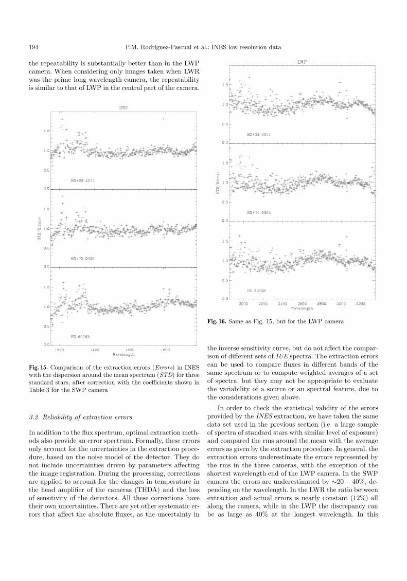
Fig. 16. Same as Fig. 15, but for the LWP camera

the inverse sensitivity curve, but do not affect the compar-ison of different sets of IUE spectra. The extraction errorscan be used to compare fluxes in different bands of thesame spectrum or to compute weighted averages of a setof spectra, but they may not be appropriate to evaluatethe variability of a source or an spectral feature, due tothe considerations given above.

In order to check the statistical validity of the errorsprovided by the INES extraction, we have taken the samedata set used in the previous section (i.e. a large sampleof spectra of standard stars with similar level of exposure)and compared the rms around the mean with the averageerrors as given by the extraction procedure. In general, theextraction errors underestimate the errors represented bythe rms in the three cameras, with the exception of theshortest wavelength end of the LWP camera. In the SWPcamera the errors are underestimated by ∼20− 40%, de-pending on the wavelength. In the LWR the ratio betweenextraction and actual errors is nearly constant (12%) allalong the camera, while in the LWP the discrepancy canbe as large as 40% at the longest wavelength. In this

P.M. Rodrıguez-Pascual et al.: INES low resolution data 195

Fig. 17. Same as Fig. 15, but for the LWR camera with a voltageof −5.0 kV

Table 3.

Camera a b

LWP −0.49 6.2 10−4

SWP 1.11 1.6 10−4

LWR(−5.0 kV) 1.12 −3.1 10−6

camera, shortward 2400 A the extractions errors are toolarge by 15− 20%. This region is very noisy and there arereasons to suspect that such a noise departs significantlyfrom a gaussian behaviour.

It is also found that the dependency of the ratioSTD/Error (where “STD” is the standard deviationaround the mean spectrum, and “Error” is derivedfrom the extraction errors) with wavelength can be wellrepresented by a straight line with the coefficients shownin Table 3. Reliable values for these coefficients could notbe obtained for the LWR camera operated at −4.5 kVdue to the scarcity of data.

In order to compare fluxes in different spectra of thesame object, the extraction errors must be modified ac-cording to

ε(λ) = a+ bεE(λ) (5)

where a and b are the coefficients in Table 3 and εE(λ) arethe extraction errors.

The results of the application of this correction areshown in Figs. 15, 16 and 17. The dispersion around theexpected value of 1 is 0.15 for SWP, 0.17 for LWP and 0.18for LWR. The structure still seen in these figures mightbe related to remaining non linearities in the ITF’s (seebelow).

3.3. Flux linearity

Despite the correction applied during the processing of theIUE data through the application of the Intensity TransferFunctions (ITFs), the final spectra are still affected bynon-linearities to some degree. As a consequence, spectraof the same non-variable object observed with differentexposure times might have slightly different flux levels.

In order to evaluate the importance of the remainingnon-linearities we have chosen, for each camera, a set oflow resolution spectra of the standard star BD+28 4211,extracted with the INES system, obtained close in timeunder similar temperature conditions and with differentexposure times. In each set one of the spectra is definedas a 100% exposure, and all the other are referred to thatone.

The summary of the data used for each camera is asfollows:

– SWP: Nine spectra taken in December 1993, with ex-posure times ranging from 2 s (9%) to 40 s (150%).

– LWP: Nine spectra taken in October 1986, with expo-sure times ranging from 10 s (20%) to 100 s (200%).

– LWR: Five spectra taken in August 1980, with expo-sure times ranging from 20 s (30%) to 150 s (250%). Allthis spectra have been processed with ITF–B (Garhartet al. 1997), which is the one giving the best correla-tion coefficient in this case, as in most of the pre-1984LWR spectra.

Each spectrum was binned into in 100 A bands and di-vided by the corresponding reference exposure. The resultsare summarized in Table 4. Examples of the behaviour ofdifferent spectral bands for each of the cameras as a func-tion of the level of exposure are shown in Fig. 18.

In the SWP camera the largest departures from linear-ity are found at the short wavelength end of the underex-posed spectra, where flux can be underestimated by up toa 20%. Apart from this case, longward Lyman α ratios tothe 100% spectrum are generally within± 5%. The bestresults are achieved in the 1800 A band, where linearity iswithin ±3%.

196 P.M. Rodrıguez-Pascual et al.: INES low resolution data

Fig. 18. Ratios of different exposure levels to the 100% for the three cameras. The thick horizontal line marks the saturated partin the overexposed spectra

For the LWP camera the largest non-linearities occurat the extreme wavelengths (1900, 3300 A), where the fluxis largely overestimated. Except for these bands, linear-ity is within ± 5% for spectra with exposure levels from40% to 150%. In the saturated region of the most exposedspectrum the flux is overestimated by 10%. Excluding thesaturated region, the bands which show the best linearitycharacteristics (within ± 3%) are those centered at 2800and 3000 A.

The LWR camera shows the largest non-linearitiesat the longest wavelengths of the underexposed spectra.Linearity remains within ± 5% for exposure levels above60%. The most linear bands are those centered at 2500,2900 and 3100 A. In the saturated part of the 200% spec-trum, the flux is underestimated by approximately 10%.However, the flux is correct in the 170% spectrum, whichis also saturated.

4. Summary

Within the framework of the development of the ESAINES Data Distribution System for the IUE FinalArchive, IUE Low Dispersion spectra have been re-extracted from the bi-dimensional SILO files with a newextraction software. INES implements a number of majormodifications with respect to the SWET extractionapplied to the early version of the IUE Final Archive.The improvements in INES deal with the noise model,the optimal extraction method, the homogenization ofthe wavelength scale and the flagging of the absolutecalibrated extracted spectra.

– The noise models for the different cameras have beenre-derived to correct anomalies at high and low expo-sure levels in those used in SWET. The noise modelresults in a considerably more realistic estimate of theactual extraction errors in the IUE spectra.

– The algorithms to compute the camera backgroundand the extraction profile are more consistent with the

P.M. Rodrıguez-Pascual et al.: INES low resolution data 197

Table 4. Linearity properties of INES low resolution spectra(ratios to 100% exposure)

SWP

Band 8% 19% 28% 39% 59% 79% 121% 151%1200 0.78 0.87 0.88 0.86 0.92 0.98 1.04 1.141300 0.81 0.90 0.87 0.92 0.96 0.99 1.03 1.041400 0.92 0.96 0.95 0.96 0.96 1.01 1.02 1.031500 0.88 0.93 0.93 0.95 0.96 0.98 0.99 0.981600 0.92 0.97 0.96 0.95 0.98 1.01 1.02 1.001700 0.83 0.99 0.97 0.97 1.00 1.02 1.03 1.001800 0.98 1.00 0.97 1.00 1.00 1.03 1.01 1.021900 0.96 0.94 0.95 0.97 1.00 1.03 1.03 1.02

LWP

Band 19% 39% 59% 79% 129% 150% 200%1900 1.33 1.28 1.04 1.11 1.03 1.03 1.012000 1.10 1.01 1.01 1.00 1.02 1.03 1.002100 1.06 1.04 1.03 1.04 1.02 1.01 1.042200 0.97 1.02 0.99 1.03 1.02 1.01 1.062300 0.97 0.98 1.00 1.00 1.02 0.99 1.012400 1.05 1.00 1.03 1.03 1.04 1.03 1.052500 1.04 1.05 0.99 0.99 1.00 1.01 1.072600 0.94 0.96 0.96 0.99 1.00 1.01 1.092700 0.95 0.96 0.99 0.99 1.02 1.05 1.122800 1.00 0.99 1.02 1.00 1.03 1.03 1.112900 1.08 1.04 1.05 1.02 1.05 1.05 1.083000 1.02 1.00 1.02 1.03 1.05 1.03 1.053100 0.93 0.99 0.95 1.01 1.07 1.05 1.023200 1.13 0.86 0.95 1.05 1.10 0.97 1.073300 1.02 1.16 1.30 1.29 1.11 1.37 1.12

LWR-ITF-B

Band 32% 56% 167% 251%1900 0.94 1.06 1.09 1.092000 0.94 1.01 1.01 1.022100 1.05 1.05 1.02 1.052200 1.01 1.00 1.02 1.022300 0.93 0.97 1.01 1.022400 1.03 0.97 1.01 1.032500 0.98 1.00 1.02 1.012600 0.97 0.98 1.02 0.902700 0.94 0.93 1.00 0.872800 0.93 0.99 1.02 0.922900 0.95 1.00 1.00 1.023000 0.99 0.95 1.01 1.053100 0.98 0.99 0.98 0.993200 1.16 1.08 1.01 1.013300 1.63 1.29 1.06 1.15

nature of the IUE detectors and result in a significantlyimproved data quality.

– Weak extended or miscentered spectra are more ade-quately handled. The fluxes of strong emission lines inweak continuum spectra are more reliable and consis-tent in the INES extraction.

– The handling and propagation of quality flags to thefinal extracted spectra has been improved. This im-plies a larger number of pixels flagged, but also a more

correct information for the user of potential problemsin the data.

– A major improvement has been reached in the removalof the solar contamination in LWP images after 1992.

– In order to facilitate an easier use of the data, all thespectra of a given range (short and long) have beenresampled to a common wavelength scale.

As a general rule, INES data are similar or superior toSWET. Although the INES spectra may at times givesomewhat lower signal-to-noise ratio than those obtainedthrough SWET (e.g. when boxcar extraction is requiredto maintain data validity), the INES extraction results ina higher reliability of the IUEFA data, allowing direct in-tercomparison of all low resolution spectra, through anadequate treatment of errors, flags and warning messagesin the image header.

Acknowledgements. We would like to acknowledge the supportof all VILSPA staff, which collaborated actively to the devel-opment of the INES system.

References

Boggess A., Carr F.A., Evans D.C., et al., 1978, Nat 275, 372Cassatella A., Ponz J.D., Altamore A., et al., 1998, in: “UV

Astrophysics beyond the IUE Final Archive”, WamstekerW. & Gonzalez-Riestra R. (eds.), ESA SP-413, p. 697

Garhart M.P., Smith M.A., Levay K.L., Thompson R.W., 1997,IUE NEWSIPS Information Manual, Version 2.0

Horne K., 1986, PASP 98, 609Huelamo N., et al., 1999 (submitted to MNRAS)Linde P., Dravins D., 1990, in: “Evolution in Astrophysics: IUE

Astronomy in the era of new Space Missions”, ESA SP-310,p. 605

Nichols J.S., 1998, in: “UV Astrophysics beyond the IUE FinalArchive”, Wamsteker W. & Gonzalez-Riestra R. (eds.),ESA SP-413, p. 671

Nichols J.S., Linsky J.L., 1996, AJ 111, 517Perez A., Pepoy J., 1997, ESA SP-1215Pian E., et al., 1997, ApJ 486, 784Rodrıguez Pascual P.M., 1993, ESA-IUE Newslett. 42, p. 1Rodrıguez Pascual P.M., Fernley J.A., 1993, ESA-IUE

Newslett. 43, p. 15Smith M.A., 1999, PASP 760, 722Talavera A., de la Fuente A., Gonzalez Riestra R., Ulla A.M.,

1992, ESA-IUE Observatory, TN8018-00