The Internet’s Dynamic Geography

Scott Kirkpatrick,School of Engineering, Hebrew University of Jerusalem

and EVERGROW

Collaborators (thanks, not blame…)Yuval Shavitt, Eran Shir, Shai Carmi, Shlomo Havlin,

Avishalom Shalit

Bremen, June 11-12, 2007

Measuring and monitoring the Internet

Has undergone a revolution Traceroute – an old hack basic tool in wide use Active monitors – hardware intensive distributed software

DIMES (“Dimes@home”) an example, not the only one now Many enhancements under consideration, as the problems in

traceroute become very evident

Ultimately, we expect every router (or what they become in the future internet) will participate in distributed active monitoring.

The payoff comes with interactive and distributed services that can achieve greater performance at greatly decreased overhead

History of TraceRoute active measurement

Jacobson, “traceroute” from LBL, February 1989 Commonly uses ICMP echo or UDP Variants exist – tcptraceroute, NANOG, “Paris traceroute” And this is something that can be rewritten for special

situations, such as cellphones Single machine traces to many destinations – Lucent,

1990s (Burch and Cheswick) Great pictures, but interpretation not clear, demonstrate

need for more analytic visualization techniques But excellent for magazine covers, t-shirts…

First attempt to determine the time evolution of the Internet First experience in operating under the “network radar”

Lumeta, their spinoff, ended up as a network radar supplier.

IP address map of August 1998

IP address map of Jan 1999

IP address map of June 1999

Map interpreted: color by ISPs

History of Internet Measurement, ctd.

Skitter and subsequent projects at CAIDA (SDSC) 15-50 machines (typically <25), at academic sites around

world RIPE and NLANR, 1-200 machines, commercial networks

and telco backbones, information is proprietary DIMES (>10,000 software agents) represents the next

step

A complementary approach is available at the coarser level of ISPs (actually “autonomous systems” or ASes)

RouteViews (Univ. of Oregon) since 2001 has monitored BGP preferred routes broadcast from a healthy sampling of ASes’ border routers.

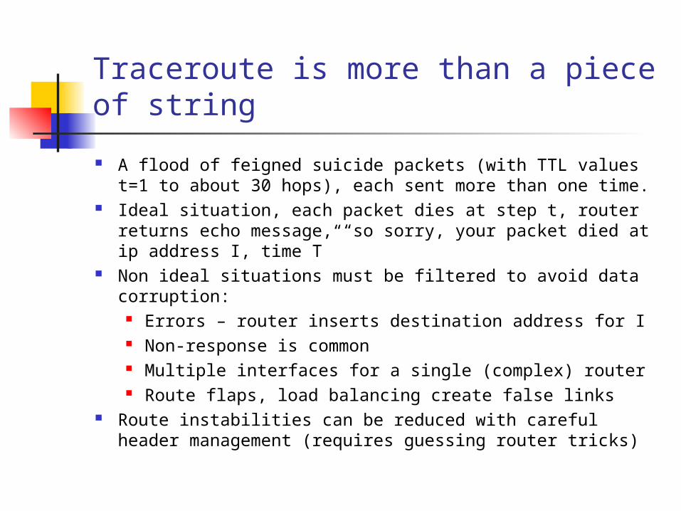
Traceroute is more than a piece of string

A flood of feigned suicide packets (with TTL values t=1 to about 30 hops), each sent more than one time.

Ideal situation, each packet dies at step t, router returns echo message, “so sorry, your packet died at ip address I, time T”

Non ideal situations must be filtered to avoid data corruption:

Errors – router inserts destination address for I Non-response is common Multiple interfaces for a single (complex) router Route flaps, load balancing create false links

Route instabilities can be reduced with careful header management (requires guessing router tricks)

The Internet is more than a random graph

Internet is a federation of subnetworks (ASs or ISPs) It has at least a two-level structure (AS, ip-level) because

two different routing strategies and software are used to direct packets. Other coarse grain views – country, city, POP…

There are no global databases, many local databases, poor data quality available.

Models have evolved steadily Waxman (Random graph with Poisson distribution of ngbrs) “Transit-stub” model with two-level hierarchy Power law pictures, such as preferential attachment, reordering Jellyfish and Medusa

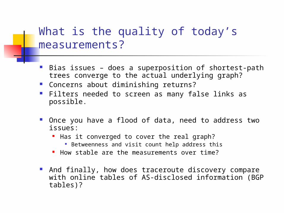
What is the quality of today’s measurements?

Bias issues – does a superposition of shortest-path trees converge to the actual underlying graph?

Concerns about diminishing returns? Filters needed to screen as many false links as possible.

Once you have a flood of data, need to address two issues:

Has it converged to cover the real graph? Betweenness and visit count help address this

How stable are the measurements over time?

And finally, how does traceroute discovery compare with online tables of AS-disclosed information (BGP tables)?

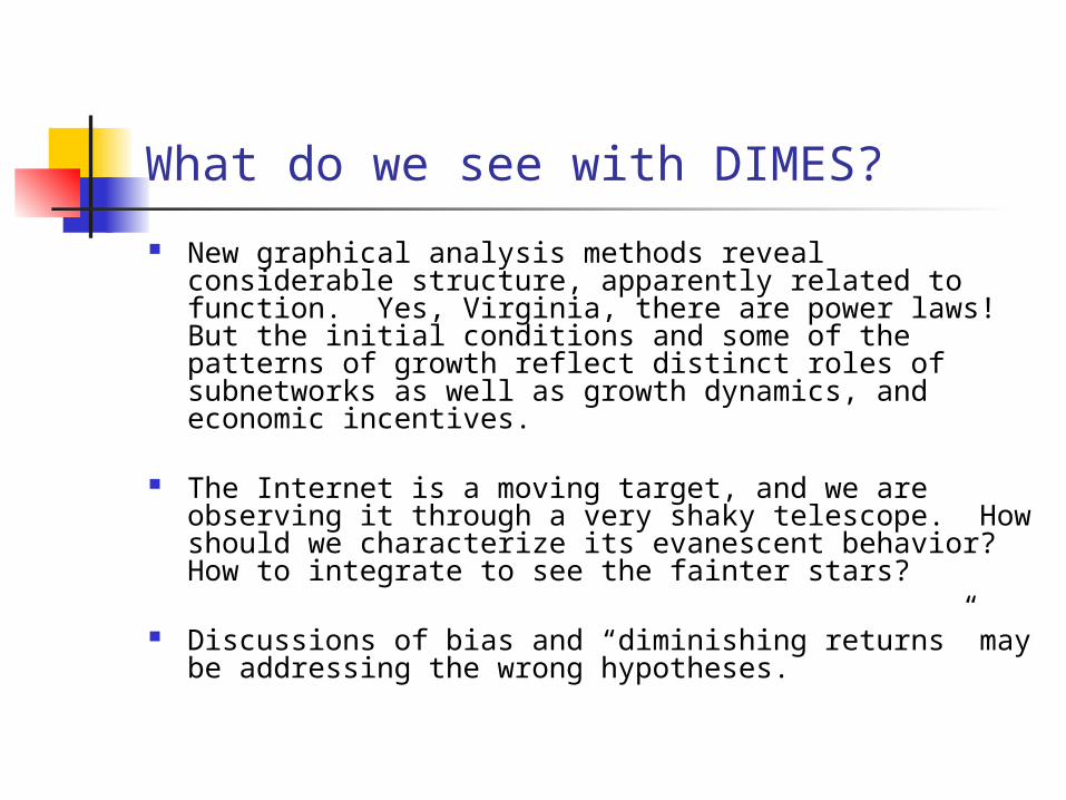
What do we see with DIMES?

New graphical analysis methods reveal considerable structure, apparently related to function. Yes, Virginia, there are power laws! But the initial conditions and some of the patterns of growth reflect distinct roles of subnetworks as well as growth dynamics, and economic incentives.

The Internet is a moving target, and we are observing it through a very shaky telescope. How should we characterize its evanescent behavior? How to integrate to see the fainter stars?

Discussions of bias and “diminishing returns” may be addressing the wrong hypotheses.

Use a new analytical tool – k-pruning

Prune by grouping sites in “shells” with a common connectivity further into the Internet: All sites with connectivity 1 are removed (recursively) and placed in the “1-shell,” leaving a “2-core” then 2-shell, 3-core and so forth.

The union of shells 1-k is called the “k-crust” At some point, kmax, pruning runs to completion.

Identify nucleus as kmax-core This is a natural, robust definition, and should apply to

other large networks of interest in economics and biology. Cluster analysis finds interesting structure in the k-crusts

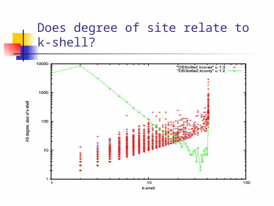
Does degree of site relate to k-shell?

Numbers of site-distinct paths in the nucleus

Conclusion: innermost k-cores are k-connected. But outer k-cores (2,3,4) show exceptions (sites with 1,2,3 paths).

kmax (03-06) = 41

kmax (05-06) = 39

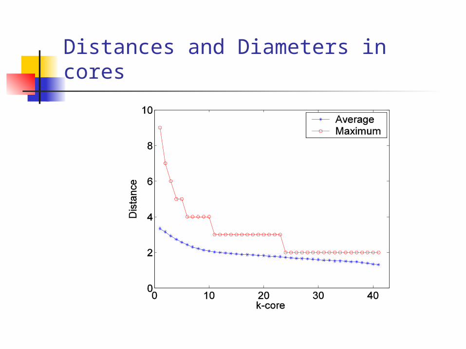
Distances and Diameters in cores

Distances and Diameters

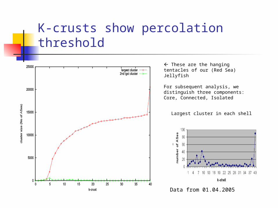
K-crusts show percolation threshold

Data from 01.04.2005

These are the hanging tentacles of our (Red Sea)Jellyfish

For subsequent analysis, we distinguish three components:Core, Connected, Isolated

Largest cluster in each shell

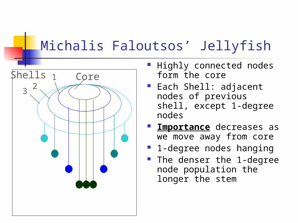
Michalis Faloutsos’ Jellyfish Highly connected nodes

form the core Each Shell: adjacent

nodes of previous shell, except 1-degree nodes

Importance decreases as we move away from core

1-degree nodes hanging The denser the 1-degree

node population the longer the stem

CoreShells 12

3

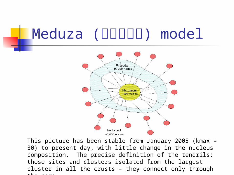
Meduza (מדוזה) model

This picture has been stable from January 2005 (kmax = 30) to present day, with little change in the nucleus composition. The precise definition of the tendrils: those sites and clusters isolated from the largest cluster in all the crusts – they connect only through the core.

Non-communication Networks

Communication networks

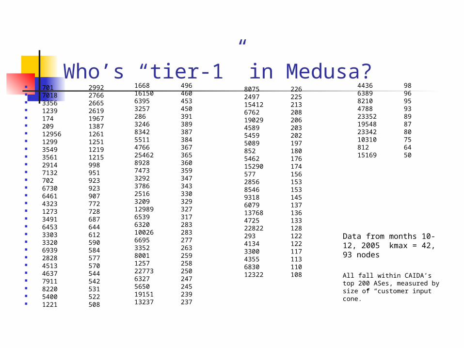
Who’s “tier-1” in Medusa? 701 2992 7018 2766 3356 2665 1239 2619 174 1967 209 1387 12956 1261 1299 1251 3549 1219 3561 1215 2914 998 7132 951 702 923 6730 923 6461 907 4323 772 1273 728 3491 687 6453 644 3303 612 3320 590 6939 584 2828 577 4513 570 4637 544 7911 542 8220 531 5400 522 1221 508

1668 49616150 4606395 4533257 450286 3913246 3898342 3875511 3844766 36725462 3658928 3607473 3593292 3473786 3432516 3303209 32912989 3276539 3176320 28310026 2836695 2773352 2638001 2591257 25822773 2506327 2475650 24519151 23913237 237

8075 2262497 22515412 2136762 20819029 2064589 2035459 2025089 197852 1805462 17615290 174577 1562856 1538546 1539318 1456079 13713768 1364725 13322822 128293 1224134 1223300 1174355 1136830 11012322 108

4436 986389 968210 954788 9323352 8919548 8723342 8010310 75812 6415169 50

Data from months 10-12, 2005 kmax = 42, 93 nodes

All fall within CAIDA’s top 200 ASes, measured by size of “customer input cone.”

What about the error bars, the bias, etc.?

Need to address the specifics of the “network discoveries”

How frequently observed? How sensitive are the observations to the number of

observers? How do the measurements depend on the time of

observation?

The extensive literature on the subject is mostly straw-man counterexamples, that show bias from this class of observation can be serious, in graphs of known structure, but do not address how to estimate structure from actual measurements.

Lecture 2 Efforts to model the Internet

Waxman (Poisson statistics, single scale) Zegura and co-workers (GaTech) two scales

“Transit” and “stub” Preferential attachment

Shalit et al (2001) showed exponent in (2,3) possible, and k-shells also give simple power laws

Counterattack of the establishment Luddites?

The Empire Strikes Back!

Willinger et al. analysis of models

Is a particular model “descriptive” or “explanatory”?

Descriptive models are “evocative “data-driven” But too generic in nature

Explanatory models are Structural Can close the loop by validating the explanatory

steps with real data “Demystify emergent phenomena”

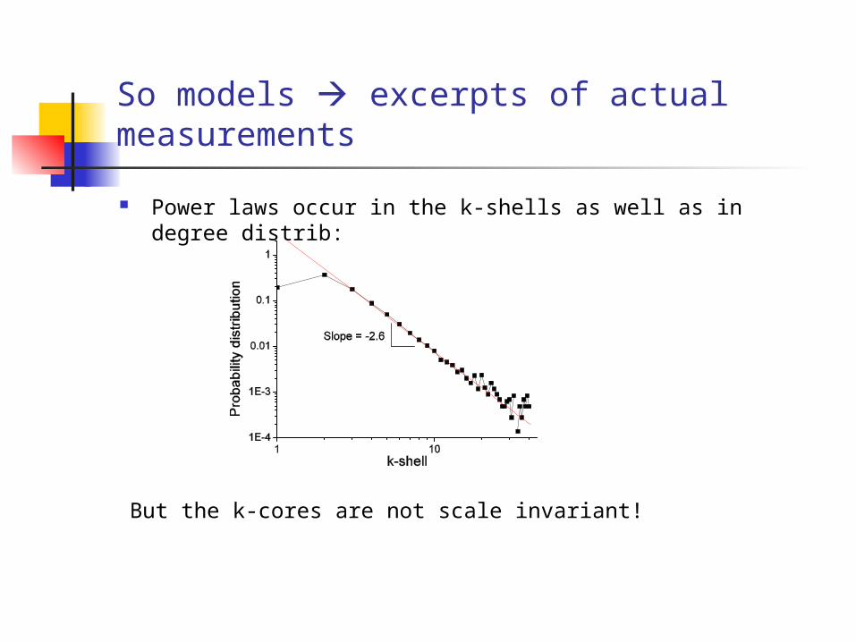
So models excerpts of actual measurements

Power laws occur in the k-shells as well as in degree distrib:

But the k-cores are not scale invariant!

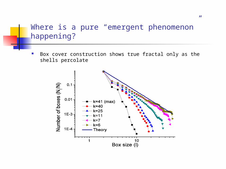
Where is a pure “emergent phenomenon” happening?

Box cover construction shows true fractal only as the shells percolate

Back to the actual data Visit count and betweenness

Best evidence for reliability of data How much better will it get with 100,000

agents observing? Can’t ask the question. But can ask, how much

worse will it be with fewer. Three approaches in prospect. All future work.

Study betweenness of present graph with reduced traffic model

Reanalyze our raw data with fewer agents included Run retrospective experiments with agents selected

specially

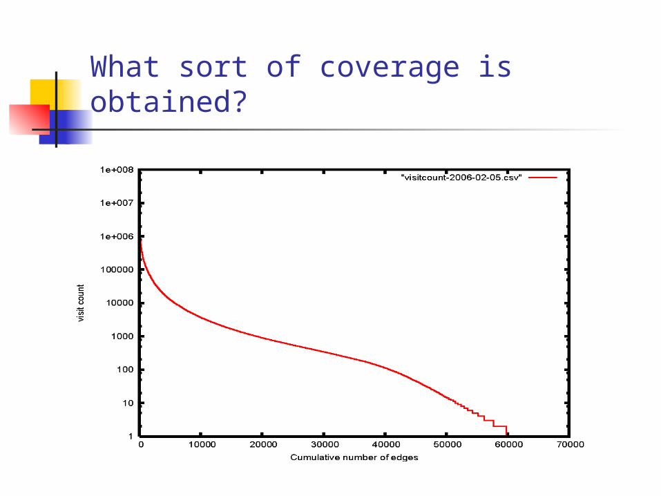
What sort of coverage is obtained?

Agents from entire two years participate

Weekly coverage and agent utilization

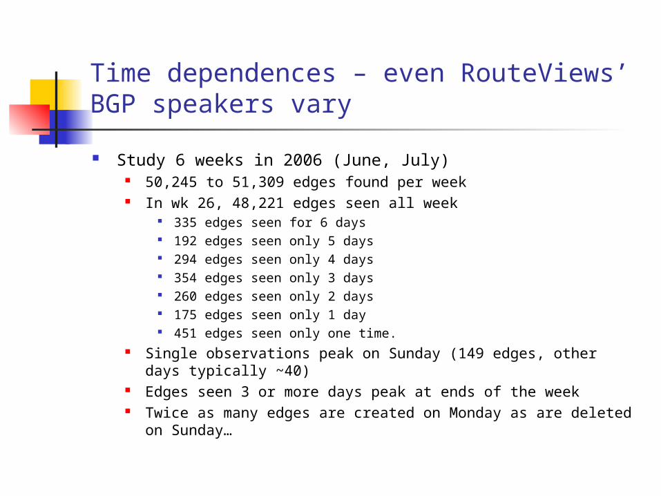
Time dependences – even RouteViews’ BGP speakers vary

Study 6 weeks in 2006 (June, July) 50,245 to 51,309 edges found per week In wk 26, 48,221 edges seen all week

335 edges seen for 6 days 192 edges seen only 5 days 294 edges seen only 4 days 354 edges seen only 3 days 260 edges seen only 2 days 175 edges seen only 1 day 451 edges seen only one time.

Single observations peak on Sunday (149 edges, other days typically ~40)

Edges seen 3 or more days peak at ends of the week Twice as many edges are created on Monday as are deleted on

Sunday…

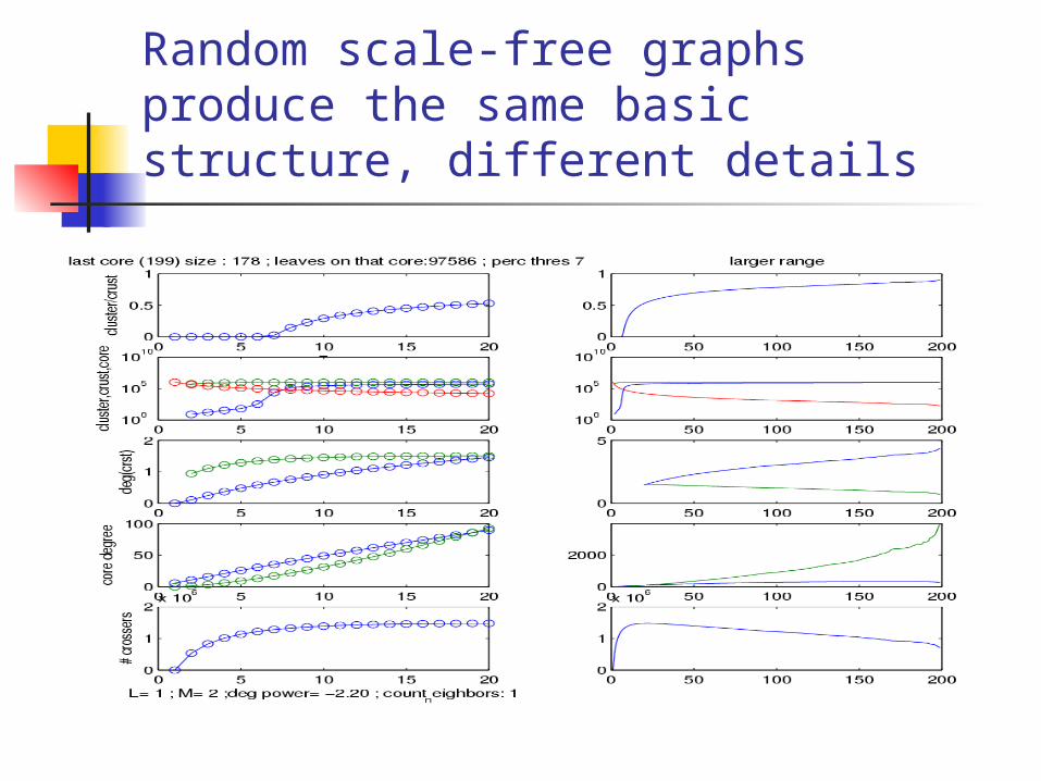
Random scale-free graphs produce the same basic structure, different details

Percolation “attacks”

K-core based attack (“by reputation”) is comparable to accurate degree-based attack for random networks, but not for the real AS graph.

Preliminary reachability data (using whole graph)

Site

s re

acha

ble

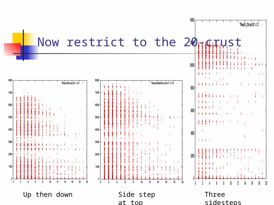
Now restrict to the 20-crust

Up then down Side step at top Three sidesteps