THE IMPACT OF WIND CAPACITY ON ELECTRICITY ...

THE IMPACT OF WIND CAPACITY ON ELECTRICITY GENERATION COSTS IN INDIANA

Clay D. Davis

Douglas J. Gotham

Paul V. Preckel

State Utility Forecasting Group

June 2013

State Utility Forecasting Group Page 1

EXECUTIVE SUMMARY

This report examines the impact of wind power on the cost of generating electricity in Indiana by comparing the load in a specific time period to the expected wind generation output at the same time period and determining the amount of energy that must be supplied from other generators. Results include the impact on both the capital costs for new generating equipment and the operating costs to generate electricity. Only costs are considered, so possible non-cost benefits of wind such as reducing risk through a more diverse portfolio are not captured.

The inclusion of wind in the generation mix has a number of cost implications, some of which lower overall costs and some that increase costs. Factors that lower cost include displacing the consumption of fossil fuels with a free source of power and displacing the need for new resources from other sources. The latter factor is somewhat complicated due to the relationship between customer load and wind speed. In general, the wind tends to be strongest during periods of the day (and seasons of the year) when load is lowest. This means that while additional wind capacity will likely reduce the total need for other types of new capacity, the impact varies by capacity type, i.e. baseload versus peaking. For the most part, adding wind reduces the need for baseload resources, which have the highest capital cost, and increases the need for peaking resources, which have a lower capital cost. Thus, adding wind not only has the benefit of reducing the total amount of incremental capacity needed, but it also reduces the total capital cost of the mix of those resources.

Factors associated with wind that tend to increase the overall cost include the capital cost of the wind generation itself, and changes in the amount that existing resources are used for generating electricity. For the same reason that baseload resource needs decrease and peaking needs increase, existing low operating cost baseload generators are used less and high operating cost peaking units are used more. Thus, while adding wind generation reduces the amount that must be generated from fossil-fueled units, what is generated tends to be at a higher cost.

In order to determine the impact of wind on overall generating costs, the new capacity requirements and economic dispatch for Indiana were determined for levels of wind capacity between 0 and 6,000 megawatts (MW). Additional scenarios were examined that attempted to look at the value of geographic diversity for the wind generators; that is, looking at wind from sites in different locations so that it is less likely that the wind would stop blowing at all sites simultaneously. In addition, the impact of including subsidies and carbon costs, which improve the relative economics of wind, were examined.

In all cases, additional wind had a capacity value in the sense that the amount of other new resources decreases as wind capacity increases. This benefit declines as the amount of wind capacity increases (the first 1,000 MW has more capacity benefit than the second 1,000 MW and so forth). Despite the capacity benefit, the total capital cost increases as wind capacity increases. This occurs because the capital cost of the wind capacity exceeds the reduction in capital costs from new fossil-fueled resources.

In all cases, there is a net reduction in operating costs as wind capacity increases. While there is a slight increase in variable costs from peaking units for small amounts of wind, it is insignificant compared to the reduction in variable costs from other units.


However in all cases, the increase in annualized capital costs exceeds the reduction in operating costs. Thus, total costs increase as wind capacity increases. The amount of the increase and its impact on electric rates depends on the amount of wind capacity and the existence of subsidies or carbon prices. In going from no wind to 1,000 MW of wind capacity, the rate impact ranges from 0.8% (with the inclusion of both a production tax credit and a relatively high carbon price) to 2.7 percent (with no tax credit or carbon cost). Moving from no wind to 6,000 MW results in rate impacts between 4.7% and 17.7% depending on the scenario.

It must be noted that there are a number of assumptions that have the potential to affect the results of this study. The study assumes capital costs and fossil fuel projections used by the Energy Information Administration (EIA). The lower natural gas price projections from EIA, which result from recent developments in capturing unconventional sources, hurts the relative economics of wind generation. Should fossil fuel prices rise above the projected levels, adding wind would result in a lower cost impact or even a cost reduction. Similarly, relative changes in the capital costs of new generators would impact the results. The study also assumes that the existing generating fleet is available. Since the existing fleet has an abundance of baseload generation, the cost benefit of reducing the need for new baseload resources that occurs with additional wind capacity is limited. As existing units are retired, adding wind would be expected to result in higher levels of capital cost reduction. Thus, the relative economics of wind would improve. The study does not consider the potential impact of price responsive demand, which could reduce the peak load levels. Pairing demand response with increased wind generation could also improve the relative economics of wind.


INTRODUCTION

Over the past few years, wind energy has become an increasingly significant component of Indiana’s portfolio of electricity supply. Given the emphasis on lower emission sources of generation resulting from tighter federal regulations, the reliance on wind energy is expected to grow in the future. Thus, understanding the impacts of including larger amounts of intermittent resources, such as wind, on the overall generation mix is important. This report examines how the inclusion of varying levels of wind power changes the capital and operating costs of generation resources for the state of Indiana.

The output of a wind generator depends on the wind speed, with higher wind speeds corresponding to more power supplied by the generator. It should be noted that a wind generator can produce electricity at a lower level than the wind speed allows, a process known as curtailment of the generator output. Wind curtailment does, however, allow the wind generator to change output between its minimum output level and the maximum output achievable at the present wind speed. Since the fuel cost of the wind generator is zero, curtailment generally results in increased system operating costs.

Another important factor for consideration is the variability of the wind. The wind speed at the wind generator changes over time, which means that the power generated by the generator changes. Holding all other factors constant (such as the loads on the system), when the wind generator output changes, some other generator must be changed in the opposite direction to keep total generation and load in balance. Of course, load levels also change over time. Thus, the dispatchable generation on the system must adjust to account for both changing load and changing wind. If wind output and load change in the same direction, the need to adjust dispatchable generation is lessened. If wind output and load change in opposite directions, the need to adjust dispatchable generation increases. Unfortunately, wind speed and load tend to be negatively correlated in the Midwest. That is, periods of relatively high wind speeds tend to correspond to periods of low load levels. Figure 1 shows the average hourly load data for the state of Indiana for the years 2004-2006 and simulated wind speed data for the same period. The wind speed data is calculated from estimates from locations in the National Renewable Energy Laboratory’s Eastern Wind Integration and Transmission Study (EWITS) that most closely correspond to locations from which Indiana utilities currently purchase wind power [NREL, 2010].


Figure 1. Average Indiana hourly load and simulated wind generation for the years 2004-2006

An increase in the amount of wind power generally results in an overall decrease in the amount of generating capacity that is needed from other sources. This occurs because there is usually some amount of wind power produced during the periods of high demand. The wind output at the time of peak demand is usually lower than it is during other times of the year. This indicates that incorporating wind into the generation portfolio has the potential to have a greater impact during off-peak periods than during the peak periods. This has important implications for the appropriate mix of fossil-fueled generators to be used in conjunction with the wind generators to meet the load. Lower off-peak loads mean that less baseload generation is needed. Baseload generation, historically coal-fired or nuclear, is characterized by relatively high capital costs and low operating costs. It is typically used during most hours of the year. Since wind power is normally greater during off-peak hours than on-peak hours, the decrease in baseload resource needs due to wind is greater than the decrease in total resource needs. This indicates that the need for other types of resources, such as intermediate or peaking, must increase. These types of resources often use natural gas and have lower capital costs but higher operating costs than baseload resources. They are used for fewer hours of the year than baseload resources.

This report examines the impact of increasing levels of wind generation on both the capital costs of new generation and the operating cost of both new and existing generation in Indiana. It uses expected demand in 2025 from the 2009 SUFG forecast [SUFG, 2009] and actual historical hourly loads that were obtained from the Indiana utilities, paired with the EWITS wind data [NREL, 2010] for the same hours, over a three-year period (2004-2006).

0

50

100

150

200

250

300

350

0

2,000

4,000

6,000

8,000

10,000

12,000

14,000

16,000

1 3 5 7 9 11 13 15 17 19 21 23

Win

d (M

W)

Load

(MW

)

Day Hour

Average LoadAverage Wind


This report is based on work from Chapter 2 of the doctoral dissertation of Clay Davis, “Three Essays on the Effect of Wind Generation on Power System Planning and Operation” [Davis, 2013] and an earlier study produced by SUFG in March 2011 [SUFG, 2011]. It includes a discussion of what assumptions and methodology have been changed from the earlier report, what the differences are between the two studies, and the significance of those differences. For more technical detail on the methodology and sensitivity analyses, please see Dr. Davis’s dissertation, which is available on the SUFG website.

METHODOLOGY

This report provides a framework for assessing the impact of wind generation on the need for other generation resources for the state of Indiana. Observed load data for 2004-2006 and estimated wind generation data from EWITS from the same time period were used to estimate the impact of wind generation on system costs and on the need for other generation types. In addition to wind, three generating technologies were considered (pulverized coal, natural gas combined cycle, and natural gas combustion turbine) for use in conjunction with existing installed Indiana generating capacity. Generating resources were classified as one of three types (baseload, cycling, and peaking). A ten percent statewide reserve margin is included for all scenarios to account for unplanned generator outages.

The impacts of increased wind generation capacity on Indiana utilities’ generation portfolios are calculated in four areas: changes in generating capacity needs for different types of fossil-fueled capacity; the change in energy (MWh) supplied by baseload, cycling, and peaking generating units; changes in capital costs due to changes in capacity requirements; and changes in variable costs resulting from changes in energy requirements.

The EWITS data consists of estimates of potential wind power output at ten minute intervals for various sites within the eastern United States. The hourly load data were linearly interpolated to ten minute intervals, so as to correspond with the wind generation data. It is important that the timing of the wind generation and load data coincide because wind speed affects both data types. For instance, higher wind speeds during the summer simultaneously results in greater wind generator output and lower air conditioning loads.

For this analysis, wind sites were chosen in close proximity to existing Indiana wind power purchase agreement (PPA) sites. The site capacities were initially scaled to the wind capacity agreed upon in the Indiana power purchase agreements. The load data for each year were scaled from the respective year up to the forecast load in 2025 (as projected in the 2009 SUFG forecast) .1 That is, each annual load profile was scaled such that annual energy consumption is equivalent to the projected consumption in 2025 (144,495 GWh). The three years of load data were all scaled to the same year (2025) in order to

1 The load level is increased to ensure that additional resources are needed so that the impact of wind on capacity needs and the corresponding impacts on capital costs are captured. The choice of forecast and forecast year are arbitrary and should not significantly affect the results as long as load levels are high enough to require additional resources.


generate three distinct annual load profiles. Impacts were calculated for each of the three years and averaged.

Calculation of Capacity Requirements and Capital Costs

Capacity requirements were calculated for the three generation resource types (baseload, cycling, and peaking) as wind capacity was added relative to a base resource case, which includes existing generation plus planned capacity changes. The base resource case capacity levels are: 16,426 MW baseload, 2,500 MW cycling, and 3,585 MW peaking.

Load duration curves (LDCs) were created by sorting the load from highest to lowest across each year. The major advantage of the LDC is that by ranking the load levels from highest to lowest, one can determine the amount of time the load is above a certain level, which is helpful in determining the appropriate amount of each of the three capacity types should be included.

In this analysis, there is no wind generation uncertainty, so that the analysis effectively assumes a perfect wind forecast. Since wind generation has near zero variable costs and wind power purchase agreement contracts are “take-or-pay” (i.e. the utility must pay for the wind generation regardless of whether it is used), all energy generated by wind units is used in the capacity planning stage. Therefore, the LDC analysis was adjusted to first remove the load that would be served by the wind generation, creating load net of wind duration curves.

Capacity levels for the three generation types were calculated using a break-even cost curve, in conjunction with the load net of wind duration curves.2 This approach of dispatching to a load net of wind duration curve ignores some features of the economic dispatch problem, such as the possibility of wind curtailment, generator minimum up and down times, and the topology of the transmission network. The advantage of determining capacity requirements in this manner is that it results in the least cost mix of generation resources to serve a given load net of wind duration curve. The break-even cost curve and load net of wind duration are shown below in Figure 2. The upper chart shows the break-even points of the three generation technologies. The vertical axis represents the annualized per unit capital cost for each of the three technologies, with baseload having the highest capital cost and peaking generation the lowest capital cost. The slope of each line represents the variable cost of the three resource types. The points where the lines intersect represent the number of hours of operation where the cost of either option is the same. Peaking generation is characterized by low capital costs and high variable costs making this resource the lowest cost form of generation for serving the highest load portion of the LDC, due to peaking generation being the lowest cost form of generation when operating a small portion of the year. Similarly, baseload generation is the lowest cost resource to serve the lowest portion of the LDC, where this resource operates for the majority of hours during the year. For

2 This methodology is different from the one used in the 2011 study produced by SUFG. The previous report used an arbitrary cutoff of the 90th percentile of the LDC for peaking capacity needs and the maximum daily load variation less the peaking capacity to determine the cycling capacity needs.


purposes of capital and operating costs in this analysis, natural gas combustion turbines (CT) were used for peaking, natural gas combined cycle units (CC) were used for cycling, and pulverized coal units (PC) were used for baseload.

Figure 2. Break-even Cost and Load Duration Curves

Due to the relatively low cost of natural gas used in the analysis (taken from the Energy Information Administration’s 2011 Annual Energy Outlook), the slope of the CT and CC lines are less than they would be with higher natural gas prices. This has the effect of moving the points where the lines cross to the right, which indicates it is economical to operate the lower capital cost option for a greater number of

Load Duration Curve

Total Cost Curve

PC

Cycling

CT

Hours per Year

Hours per Year

Peaking

CC

Baseload


hours. In fact, the CC curve falls below the PC curve for all hours of the year. In other words, it would be cheaper to construct and operate a new natural gas combined cycle facility than a new pulverized coal facility, even if the units were operated 100 percent of the time. Thus, the natural gas combined cycle option is the appropriate choice for both new cycling and baseload capacity.3 Figure 3 illustrates the break even cost curve for lower natural gas prices.

Figure 3. Break-even Cost and Load Duration Curves with Low Natural Gas Prices

3 Since pulverized coal may be economic under a different set of fuel prices, it is included in the model. The operational parameters assumed for pulverized coal units are included in this report even though it is not economical under the fuel prices used.

Load Duration Curve

Total Cost Curve

PC

CT

Hours per Year

Hours per Year

Peaking

CC

Cycling and

Baseload


Capacity requirements for the three generation resources were calculated for the load net of wind duration curves. The new capacity requirements to meet 2025 demand were determined by subtracting the existing capacity levels (3,585 MW of peaking capacity, 2,500 MW of cycling capacity, and 16,426 MW of baseload capacity) from the levels resulting from these calculations. If the baseload capacity requirement is less than 16,426 MW, then no new baseload capacity is necessary and the excess existing baseload capacity is reclassified as cycling capacity. Similarly, if no new cycling capacity is needed then both excess baseload and cycling capacity are reclassified as peaking capacity. This reclassification may become more prevalent as wind capacity increases and is necessary to avoid adding new capacity while there is idle existing capacity. The 2025 new capacity levels calculated for each generation resource type were further increased by ten percent to account for forced outages. These capacity levels were used when dispatching the ten minute load, in order to calculate the energy impacts.

Capital costs for this analysis are on an annual basis. Baseload capacity is modeled using characteristics representative of a pulverized coal plant, cycling capacity as a combined-cycle gas turbine unit, and peaking capacity as a combustion turbine unit. Per unit annualized capital costs of these technologies, as well as wind generation are shown below in Table 1. These costs include annualized capital costs plus fixed operating and maintenance costs associated with generation.

Table 1. Annualized Capital Costs and Variable Costs by Generation Typea

Unit Vintage Generation Type Annualized Capital Cost (2010 $/MW/Yr)

Variable Cost (2010 $/MWh)

New Units PC 542,277 25.34 CC 170,100 37.66 CT 110,353 62.26 Wind 403,430 0.00 Existing Units Baseload n.a. 24.65 Cycling n.a. 42.72 Peaking n.a. 67.27 Wind n.a. 0.00

a Fixed costs for baseload, peaking, cycling and wind units are from Tables 3-3, 9-2, 6-2 and 21-2 respectively, using

Indiana specific costs [EIA, 2010]. Capital costs for existing units are sunk costs and hence, not used in the analysis. Fuel costs are 2025 projections for the East North Central Region in the EIA 2011 Annual Energy Outlook (EIA, 2011). Fuel prices are in 2010 dollars. Variable O&M costs and plant characteristics for existing generation are from typical Indiana generating units. Variable costs for wind are treated as zero.

Calculation of Energy Impacts and Variable Costs

Energy impacts were calculated using a minimum cost economic dispatch model with wind generation being dispatched in addition to the other three non-wind generation technologies to meet load for each ten minute interval. The model minimizes the cost of meeting demand in each time period. Wind


generation may be dispatched up to the level of wind generation for a given ten minute interval, allowing for the possibility of wind curtailment when it is optimal. The other three generation technologies may be dispatched up to the capacity levels determined from the capacity planning stage for the various levels of wind capacity. If some wind generation is curtailed in the economic dispatch model it would alter the shape of the load net of wind duration curve and may have an impact on the optimal capacity. While wind curtailment would alter the load net of wind duration curve (and the optimal mix of generating capacities), this effect is expected to be minor. Absent any wind curtailment the energy impact from wind generation is equal to the total wind output for the year, although variations in impacts are likely across the three generation technologies. Additionally, ramping limits are imposed on baseload, peaking, and cycling generation.4 Ramping limits are shown by generation technology in Table 2 and are specified as a percent of installed capacity because the number of generating units is not determined in this analysis. Wind curtailment will only take place to avoid violating a ramping limit. Other reasons wind curtailment may take place in a wholesale market, which were not modeled in this analysis, are to avoid violating transmission constraints, wind generation forecasting errors, or wind generation not having a lower offer price than the offer price of the marginal generation unit.

Energy impacts were calculated as the difference in generation for each technology between the base (no wind) case and generation at various levels of installed wind capacity. The difference in energy supplied by baseload capacity for the load and load net of wind profiles determines the change in energy that must be supplied by baseload generation at a given level of wind capacity. Similar calculations determine wind generation impacts on cycling and peaking generation. Again, these calculations were made for all three years and then averaged to arrive at an expected energy impact.

Table 2. Generator Ten Minute Ramping Limits as a Percent of Installed Capacitya

Unit Vintage Generation Type Ramping Limit (% of capacity)

New Units PC 40 CC 70 CT 100 Wind 100b Existing Units Baseload 10 Cycling 60 Peaking 100

a Baseload ramping limits p. 6 [Ihle, 2003]; Cycling ramping limits Table 1 [NWPP, 2002]; Peaking is assumed to have a ramping limit of 100 percent of installed capacity. b Wind generation is capable of ramping between zero and the level of wind generation available for that ten minute period, as opposed to a percent of installed generation capacity.

4 Ramping limits were not included in the 2011 study due to the use of 1-hour time steps in the model at that time (as opposed to 10-minute time steps now). Many units are not able to fully ramp between minimum and maximum output in a ten minute period but can do so in an hour.


Variable costs were broken down by generation type and listed separately for new and existing capacity. This further distinction is made because newer technologies are generally more efficient due to lower heat rates, resulting in lower variable costs. Per unit variable costs are equal to per unit fuel costs plus per unit variable operations and maintenance costs (see Table 1). Wind generation is assumed to have zero variable cost.

Total variable cost impacts for a given level of wind capacity were calculated relative to total variable costs by generation type without any wind generation. For example, the impact for new peaking variable cost is calculated as the difference between energy supplied by new peaking capacity without wind versus energy supplied by new peaking capacity given a specific level of wind generation, multiplied by new peaking variable cost. This calculation is performed for both new and existing units by type of generation and summed to arrive at the total impact. This is the annual impact for the year 2025, and it is calculated based on the data for each of the three years and then averaged to get the expected impact.

Modeling Scenarios

The impact of increasing levels of wind generation was captured by varying the wind generation in the Indiana portfolio from 0 to 6,000 MW. The physical locations of the wind generators have some impact on the results, since some sites have greater average wind speeds while others may provide greater diversity in wind output. That is, when there is little to no output at existing sites, some alternative sites may be more likely than others to be producing at a higher level. Four scenarios were chosen to show some key differences between adding wind at alternative locations in different regions. The results of the four scenarios chosen show that the location from which wind power is sourced is important, but also that the proportion of the wind capacity from a particular location in the overall wind portfolio is important, as well. The four scenarios modeled in order to further draw out these distinctions are: 1) scaling all power purchase agreements (PPAs) in proportion to their existing level, 2) scaling in-state PPAs in proportion to their existing levels while holding out-of-state PPAs constant, 3) scaling out-of-state PPAs in proportion to their existing levels while holding in-state PPAs constant, and 4) equally scaling all existing PPAs and the five sites in Indiana that are least correlated with the existing PPAs.

The first scenario scales all existing power purchase agreements in proportion to their existing levels. This has the effect of adding more wind capacity at sites that currently have a higher share of Indiana wind capacity and less at sites that currently have a lower share of wind capacity. For example, if two sites currently have 100 MW and 300 MW of wind capacity, then adding 100 MW of wind capacity will result in adding 25 MW at the 100 MW site and 75 MW at the 300 MW site. If the sites that currently have the most capacity are more likely to have wind additions than sites that currently have less capacity, then this scenario models that reality.

The second scenario scales all in-state wind sites proportionally in the same manner as the first scenario, while holding out-of-state sites at their existing levels. The third scenario scales the out-of-state sites proportionally, while holding the in-state sites at existing wind capacity levels. Scaling the first three


scenarios in this way shows the impacts resulting from changes in proportions of in-state and out-of-state sites.

The last scenario is intended to show the benefits from additional geographic diversification of the wind portfolio. Adding the five least correlated sites to the existing wind sites is intended to reduce the variability of the total wind portfolio. Reducing this variability should decrease the capacity needs of other resources. Instead of scaling all sites in proportion to their existing levels, the capacity levels of existing sites and five new sites are all increased equally in MW terms. Since the scaling was done in a manner that did not hold the proportion of each site in the overall portfolio constant, impacts are the result of diversification and a changing portfolio make-up.

Again, these scenarios are intended to show the importance of location when choosing new wind sites and the portion each site comprises of the state’s overall wind portfolio. The scenarios presented here are indicative of the likely impacts of adding wind PPAs from locations that are: in-state, out-of-state, or both, as well as the fourth scenario that opportunistically selects sites that are least correlated with existing wind sites.

RESULTS

Scaling Existing PPAs (Scenario 1)

This section details the impacts of scaling wind capacities at the sites of all existing power purchase agreements in proportion to their existing levels. Total resource needs from non-wind resources decrease with increasing wind capacity, as is shown in Figure 4.5 However, there is a shift in the composition of resource needs with peaking capacity requirements increasing and baseload and cycling requirements decreasing with increasing wind capacity. The increase in peaking requirements as wind generation is added to the system is due to the increasing variation in the annual load net of wind generation profile. Increasing levels of wind generation cause the load net of wind duration curve to become steeper resulting in increasing levels of peaking capacity to become cost effective relative to cycling and baseload capacity. Beyond 2,500 MW of installed wind capacity new peaking capacity requirements begin to decrease as excess baseload and cycling capacity are dispatched as peaking capacity so as to avoid idling existing cycling and peaking capacity.

5 In Figure 4, new combined cycle capacity represents both cycling and baseload resources. No pulverized coal resources are included because of the lower cost of natural gas-fired combined cycle generation. New combustion turbine capacity represents peaking resources.


Figure 4. New Capacity Requirements

Scaling wind capacity from 0 MW to 1,000 MW offsets only 271 MW of capacity requirements from other resources. As additional wind resources are added, capacity benefits continue to exist, but at a declining rate. For instance, adding another 2,000 MW of wind resources only reduces capacity resources from other resources by 357 MW.

Annualized capital costs, in aggregate, increase with wind capacity. These costs are nearly completely driven by the capital costs of increasing wind capacity (see Figure 5). Incremental capacity costs mirror the pattern in Figure 4. Combined cycle capacity costs decrease due to a reduction in required additions. Capital costs associated with combustion turbines increase until about 2,500 MW of installed wind capacity and then decrease.

-1,000

0

1,000

2,000

3,000

4,000

5,000

6,000

7,000

8,000

0 1000 2000 3000 4000 5000 6000

Cap

acity

(MW

)

Wind Capacity (MW)

CT CC PC Total


Figure 5. Annualized Capital Costs for New Resources

As expected, energy supplied by resources other than wind decreases with increases in wind capacity. As with capacity requirements, energy that is supplied by baseload and cycling units is reduced as wind capacity increases, while energy supplied by peaking generation increases slightly as wind capacity increases up to about 2,500 MW and then declines with further increases in wind capacity (see Figure 6). Energy supplied by peaking capacity decreases beyond 2,500 MW of installed wind capacity due to the energy supplied for peaking purposes by existing cycling and baseload capacity which are not needed to meet non-peaking needs. Energy supplied by baseload and cycling generation decreases as wind penetration increases due to additions in wind capacity causing a steepening of the load duration curve. Since additions in wind capacity are not able to offset non-wind resource needs on a one to one basis the system capacity factor declines (generation resources are less utilized). The capacity factor is the ratio of how much electricity is generated given a particular level of capacity divided by the amount of electricity that could have been generated if the unit was operating at full capacity continuously, with a larger number representing more generation per unit of capacity.

0

500

1,000

1,500

2,000

2,500

3,000

3,500

0 1000 2000 3000 4000 5000 6000

Cap

acity

Cos

t (m

illio

n 20

10 $

/yr)

Wind Capacity (MW)

CT CC PC Wind Total


Figure 6. Change in Energy Requirements (Relative to No Wind Generation)

Increasing wind capacity results in substantial decreases in variable costs because variable costs associated with wind generation are treated as zero in this analysis (see Figure 7). Thus, changes in energy requirements net of wind drive the changes in variable costs. Variable costs associated with baseload and cycling generation decrease with increasing wind capacity. Variable costs for peaking generation initially increase modestly and then decrease as it is displaced by lower variable cost baseload and cycling capacity.

Figure 7. Change in Variable Costs (Relative to No Wind Generation)

-24,000

-19,000

-14,000

-9,000

-4,000

1,000

0 1000 2000 3000 4000 5000 6000

Ene

rgy

(GW

h/yr

)

Wind Capacity (MW)Peak Cycle Base Total

-700

-600

-500

-400

-300

-200

-100

0

100

0 1000 2000 3000 4000 5000 6000

Var

iabl

e C

ost (

mill

ion

2010

$/y

r)

Wind Capacity (MW)Peak Cycle Base Total


Table 3 summarizes impacts at varying levels of wind capacity.6 The capacity requirements impact represents total capacity needs, including existing capacity by resource in 2025 for a given level of wind capacity. The energy impact is energy that must be supplied by each resource type in 2025. The variable cost impact represents variable costs by resource type in 2025. Capital costs are annualized capital costs in 2025 for capacity needs relative to existing capacity.

Table 3. Annual Capacity, Energy, and Costs for Alternative Wind Capacity Levels

Impact Area

0 MW Wind

Capacity

1,000 MW Wind

Capacity

3,000 MW Wind

Capacity

6,000 MW Wind

Capacity

New Capacity Combined Cycle (MW) 875 500 0 0 Combustion Turbine (MW) 5,769 5,873 6,016 5,586 Wind (MW) 0 1,000 3,000 6,000 Energy Baseload (GWh) 126,226 125,136 122,228 116,109 Cycling (GWh) 13,424 11,238 7,981 5,836 Peaking (GWh) 4,718 4,803 4,585 3,275 Total (GWh) 144,368 141,177 134,794 125,220 Variable Cost Baseload (million $) 3,111 3,085 3,013 2,862 Cycling (million $) 550 467 341 249 Peaking (million $) 295 300 286 205 Total (million $) 3,956 3,852 3,640 3,316 Annualized Capital Cost for New Capacity Combined Cycle (million $) 149 85 0 0 Combustion Turbine (million $) 637 648 664 616 Wind (million $) 0 403 1,210 2,421 Total (million $) 786 1,136 1,874 3,037

The transition from no wind to 1,000 MW of wind results in a decrease of $104 million in variable costs. This occurs because the reduction in the amount that is generated from baseload and cycling units more than overcomes the slight increase in peaking energy. At the same time, less new combined cycle capacity is needed ($64 million worth on an annualized basis) and slightly more combustion turbine capacity is needed, causing an annualized cost increase of $11 million. The annualized cost of the wind is $403 million. The total increase in annualized capital cost is $350 million. The decrease in variable costs is not enough to overcome the increase in capital costs. Thus, the net cost of adding the wind is $246 million. Figure 8 shows the total cost impact of varying levels of wind.

6 These results do not include the federal Production Tax Credit (PTC). The impact of the PTC is included later in the report.


Figure 8. Cost Changes across Varying Levels of Wind Capacity

Comparison of Geographic Scenarios

This section compares the impacts of scaling up wind capacity across the four scenarios. The results show that while one scenario may result in a larger impact in one area, another may show a larger impact in another area. Also, while one scenario may result in the largest impact at a lower level of wind capacity another may show a larger impact at a higher level of wind capacity. This indicates that the locations of the wind capacity additions are important to the analysis.

At higher wind capacity levels, Scenario 4, existing PPAs plus the five least correlated sites, results in the largest reduction in the need for new non-wind generating capacity. This scenario is slightly superior to the scenario where all PPA sites are scaled proportionally, showing that a larger impact is achieved due to the additional geographic diversification. Scenario 2, where only in-state sites are scaled, causes the in-state sites to dominate the portfolio at higher wind penetration levels. This negates some of the benefit from geographic diversification and thus the scenario results in the smallest impact on capacity requirements. Scenario 3, where out-of-state sites are scaled up, had the second lowest capacity impact.

The total energy impacts are similar across Scenarios 1 through 3. Scenario 3 results in the largest energy impact, but the differences between the cases are small in terms of the change in energy requirements. This scenario exhibits the largest impact because the out-of-state sites have slightly higher capacity factors than the in-state sites. As this scenario is scaled up, the out-of-state sites make-up a larger portion of the overall wind portfolio. A larger capacity factor for the out-of-state sites means that a given level of wind capacity installed at an out-of-state site will result in a larger energy reduction than the same level of capacity installed at an in-state site. While the out-of-state scenario has the

-1000

-500

0

500

1000

1500

2000

2500

0 1000 2000 3000 4000 5000 6000

mill

ion

2010

$/y

r

Wind Capacity (MW)Variable Cost Capital Cost Total Cost


highest energy impact, it was shown earlier that it has the second lowest impact on capacity. This is because the out-of-state wind portfolio results in more wind generation, but during lower load periods, compared to Scenarios 1 and 4. Scenario 4 has the smallest reduction in energy requirements because the sites, which were chosen based on correlation with existing sites, have the lowest capacity factor. While wind curtailment was allowed in the economic dispatch model wind generation was not curtailed under any scenario or wind capacity level, therefore all differences in the impacts on total energy are the result of differences in capacity factors at the various wind sites.

Generally a wind site that is more highly correlated with load will have a larger impact on capacity, while a site with a larger capacity factor will result in a larger impact on energy, though this may not always be true. It would be possible for a site to have such a large capacity factor relative to another site that even if it was less correlated with load it could still lead to a larger capacity impact. This could happen if the capacity factor was sufficient to make the wind generation from the site higher during on-peak times despite being less correlated with load. Another way a site that is highly correlated with load could result in a smaller reduction in capacity would be if this site had a single, rather anomalous hour with very low output, which happened to be a relatively high load hour. As this discussion has shown, the impact of the correlation between wind generation and load and the wind site capacity factor cannot be considered entirely separate from each other.

The capital costs are nearly identical across scenarios and are driven by the capital costs from additional wind capacity. For all scenarios, this is due to the incremental costs for installing wind capacity outweighing any other changes in capacity costs. Scenario 4, which has the largest reduction in capacity, also results in the smallest increase in capital costs, $3,011 million at 6,000 MW of wind capacity as compared to the $3,037 million shown in Table 3. Scenario 2 has the highest capital costs, with an increase of $3,073 million in annualized costs at 6,000 MW of wind. It should be noted that it may not always be the case that the scenario that has the largest impact on capacity requirements will result in the smallest increase in capital costs because both the resource mix and peak load are affected. While offsetting more capacity is generally better, it is also important to consider the type of unit the additional wind capacity is replacing.

While Scenarios 1 through 3 have nearly identical energy impacts, Scenario 2 has a smaller reduction in variable costs than the other two. This result occurs because Scenario 2 displaces more of the low variable cost baseload generation and less of the high variable cost peaking generation than the other scenarios. Scenarios 2 and 4 have nearly identical variable costs despite having different energy impacts. Two factors are driving the effect on variable cost. They are the reduction in total energy and the type of generation this reduction affects, because one MWh supplied by a baseload unit has a lower variable cost than one MWh supplied by a peaking unit. The first factor affects the energy impact, while both factors affect the variable cost impact. Thus, it is the change in composition of the generating units that makes the effect on variable costs different across scenarios while the effects on energy are quite similar.

These comparisons across scenarios highlight some key characteristics of wind generation. First, while one scenario may result in the largest impact in one area (e.g. capacity, energy, or cost) it may not in


another area. This means that it is important to define the ultimate goal of the wind capacity that is being added to the system. However as a general rule, it will usually be most advantageous to add wind capacity at sites with high capacity factors and high correlation with load. Table 4 summarizes the changes in costs for moving from no wind to various levels of wind capacity using the four geographic scenarios. Scenarios 1, 3, and 4 exhibit almost identical total costs but arrive there via different routes. The scenario that relies on out-of-state sites (Scenario 3) generates the most energy from wind while the one that relies on sites that are least correlated with existing sites requires the lowest investment in other generation resources. Scenario 2, which relies on in-state sites, results in the highest total cost.

Table 4. Change in Costs across Scenarios (Relative to No Wind)

Change in Costs 1,000 MW 3,000 MW 6,000 MW Variable (million $)

Scenario 1 -104 -316 -640 Scenario 2 -104 -309 -617 Scenario 3 -105 -318 -642 Scenario 4 -103 -301 -612

Annualized capital (million $) Scenario 1 351 1,089 2,252 Scenario 2 354 1,104 2,288 Scenario 3 351 1,088 2,253 Scenario 4 349 1,074 2,226

Total (million $) Scenario 1 247 773 1,612 Scenario 2 250 795 1,671 Scenario 3 246 770 1,611 Scenario 4 246 773 1,614

Impact of Subsidies and Carbon Costs

The results presented to this point do not include some factors that may positively impact the economic competitiveness of wind generation, such as the federal Production Tax Credit (PTC) or limitations or costs associated with the emission of carbon dioxide (CO2). This section examines the impact of subsidies like the PTC and the inclusion of a price for CO2 emissions.

Numerous estimates exist for the price of CO2 emissions. The carbon prices considered in this section were derived from the Bingaman bill proposed in the U.S. Senate [Bingaman, 2011]. The bill proposes a price ceiling of $25/ton and a price floor of $10/ton for calendar year 2012, which were discounted to 2010 levels for this analysis. The price ceiling will increase each year by five percent in real terms. The carbon price ceiling of $25/ton in 2012, increasing at a rate of five percent per year in real terms, will result in a ceiling of 44.13 $/ton (2010 $) in 2025. Similarly, the price floor will increase at a rate equal to three percent per year in real terms. This yields a carbon price floor of 10 $/ton in 2012 that rises to 13.75 $/ton (2010 $) by 2025. For modeling purposes, these low and high carbon prices were converted


to dollars per megawatt hour based on heat rate, fuel type, and carbon emissions of the fuel, and are listed below in Table 5.

Table 5. Carbon Price by Type of Generation

Capacity Type

Low Carbon Price (2010 $/MWh)

High Carbon Price (2010 $/MWh)

New Capacity PC 15.47 49.65 CC 5.19 16.65 CT 7.86 25.24 Base Case Capacity Baseload 16.17 51.90 Cycling 6.31 20.24 Peaking 9.66 31.01

Baseload generation is modeled using the characteristics of a pulverized coal unit, which emits the highest levels of carbon dioxide. Cycling units, modeled using natural gas fired combined cycle technology, emit the lowest levels of carbon dioxide among the fossil fuel technologies. Cycling units have the lowest emission levels because this type of generation combines a gas turbine and steam turbine, where the exhaust heat from powering the gas turbine is then used to power the steam turbine, resulting in highly efficient generation. This highly efficient generation of combined cycle units uses less natural gas per MWh and ultimately emits less carbon dioxide per MWh. Peaking units are modeled as combustion turbine units, resulting in emissions per MWh between baseload and cycling units. It should be noted that the inclusion of carbon prices will affect the break even cost curves shown previously in Figures 2 and 3. Carbon prices will increase the variable cost of each type of unit, which will cause the slopes of the lines associated with the technologies to increase. The slope of the pulverized coal technology will increase the most since it has the highest carbon cost per MWh. Thus, for the natural gas prices in this study, pulverized coal remains uneconomical at all capacity factors and is not selected as a new resource.

Five additional sensitivities are derived from the various combinations of subsidies (with and without) and carbon prices (none, low, and high).7 These sensitivities were performed off of the first geographic sensitivity, where all existing PPAs were scaled to meet the level of wind generation. Inclusion of the PTC subsidy improves the relative economics of wind by reducing the variable cost of the entire system by the amount of the tax credit. Inclusion of a carbon cost improves the relative economics of wind by increasing the variable costs of fossil-fueled generation, thereby causing wind to displace more expensive generation. While all sensitivities had smaller cost increases with a given level of wind than are seen in the previous scenarios (no subsidy, no carbon cost), no combination of subsidy and carbon cost produces a lower total cost with wind than without. Capital costs increase faster than variable

7 The no carbon price, no subsidy case was presented in the previous sections.


costs decline at all levels of wind capacity. The reduction in variable cost due to increases in wind generation is not sufficient to offset the increases in capital costs even when the combination of the subsidy and high carbon price act to increase the reduction in variable costs.

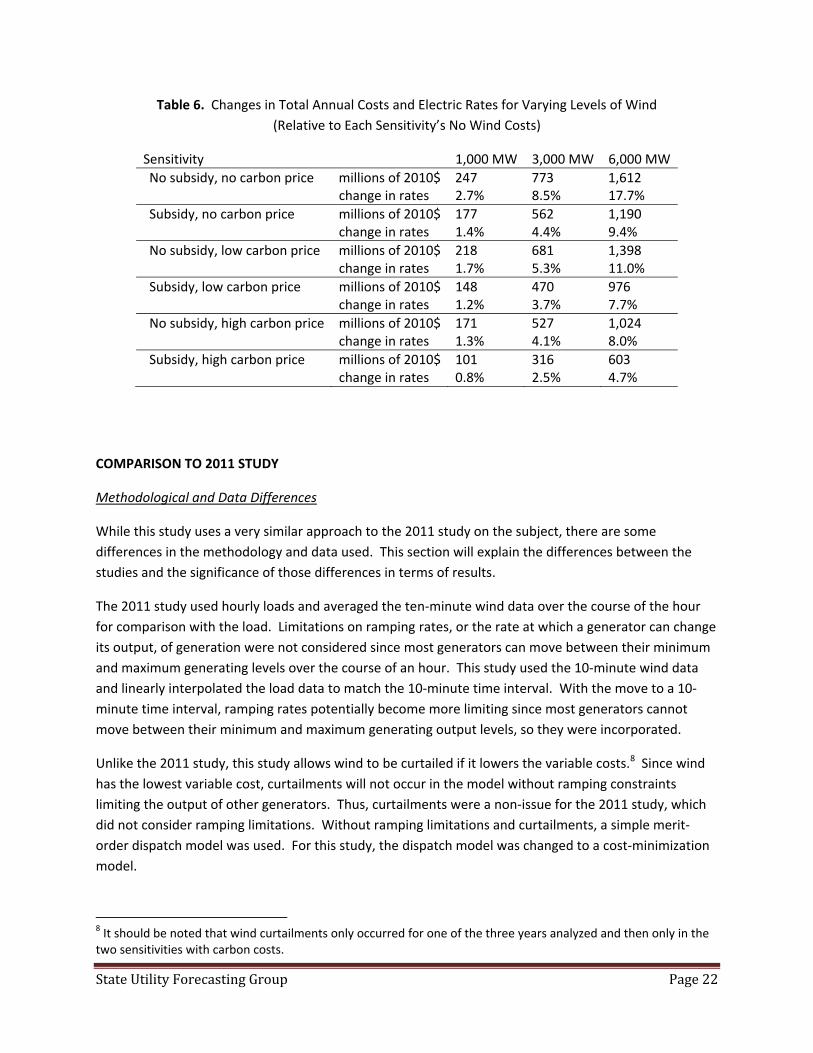
Figure 9 shows the changes in cost at various levels of wind capacity for the five sensitivities. It is important to note that the line for a particular sensitivity represents the change in cost from the no wind case under its own rules, not necessarily from the no wind case presented previously. That is, the low and high carbon costs will have higher costs with no wind than will occur without a carbon price. The low CO2 price with no PTC subsidy has the largest cost increase as wind is added, followed by the no carbon cost with subsidy. As expected, the high carbon cost with subsidy sensitivity has the lowest cost increase due to wind additions. Table 6 provides the total cost numbers for the five sensitivities and the no subsidy, no carbon case for 3 different levels of wind generation. The table also shows the percentage increase in electricity rates (from the SUFG 2025 forecast load and prices) indicated by the cost change [SUFG, 2011].

Figure 9. Change in Total Costs for Varying Levels of Wind (Relative to Each Sensitivity’s No Wind Costs)

0

200

400

600

800

1,000

1,200

1,400

1,600

0 1000 2000 3000 4000 5000 6000

mill

ion

2010

$/y

r

Wind Capacity (MW)Subsidy Low CO2 High CO2Sub. & Low CO2 Sub. & High CO2


Table 6. Changes in Total Annual Costs and Electric Rates for Varying Levels of Wind (Relative to Each Sensitivity’s No Wind Costs)

Sensitivity 1,000 MW 3,000 MW 6,000 MWNo subsidy, no carbon price millions of 2010$ 247 773 1,612 change in rates 2.7% 8.5% 17.7% Subsidy, no carbon price millions of 2010$ 177 562 1,190 change in rates 1.4% 4.4% 9.4% No subsidy, low carbon price millions of 2010$ 218 681 1,398 change in rates 1.7% 5.3% 11.0% Subsidy, low carbon price millions of 2010$ 148 470 976 change in rates 1.2% 3.7% 7.7% No subsidy, high carbon price millions of 2010$ 171 527 1,024 change in rates 1.3% 4.1% 8.0% Subsidy, high carbon price millions of 2010$ 101 316 603 change in rates 0.8% 2.5% 4.7%

COMPARISON TO 2011 STUDY

Methodological and Data Differences

While this study uses a very similar approach to the 2011 study on the subject, there are some differences in the methodology and data used. This section will explain the differences between the studies and the significance of those differences in terms of results.

The 2011 study used hourly loads and averaged the ten-minute wind data over the course of the hour for comparison with the load. Limitations on ramping rates, or the rate at which a generator can change its output, of generation were not considered since most generators can move between their minimum and maximum generating levels over the course of an hour. This study used the 10-minute wind data and linearly interpolated the load data to match the 10-minute time interval. With the move to a 10-minute time interval, ramping rates potentially become more limiting since most generators cannot move between their minimum and maximum generating output levels, so they were incorporated.

Unlike the 2011 study, this study allows wind to be curtailed if it lowers the variable costs.8 Since wind has the lowest variable cost, curtailments will not occur in the model without ramping constraints limiting the output of other generators. Thus, curtailments were a non-issue for the 2011 study, which did not consider ramping limitations. Without ramping limitations and curtailments, a simple merit-order dispatch model was used. For this study, the dispatch model was changed to a cost-minimization model.

8 It should be noted that wind curtailments only occurred for one of the three years analyzed and then only in the two sensitivities with carbon costs.


Another methodological change between the two studies involves the determination of new resource requirements. This study uses the break-even cost curve approach illustrated in Figures 2 and 3. The previous study used an arbitrary cutoff of the 90th percentile of the LDC for peaking capacity needs and the maximum daily load variation less the peaking capacity to determine the cycling capacity needs. The remaining capacity needs were classified as baseload.

While much of the data is unchanged between the two studies, there are two important differences. Updated capital cost and operating characteristics for new generation were used based on the RW Beck report produced for the Energy Information Administration [EIA, 2010]. For the natural gas-fired technologies, these costs are somewhat lower than those used previously. The wind capacity price is similar to the previous study. More recent fuel price projections were used from the 2011 Annual Energy Outlook [EIA, 2011]. The most significant change was lower expected natural gas prices.

Differences in Results

Despite the updates in methodology and data, the results of the two studies are quite similar, with wind generation faring slightly worse economically in this study. Table 7 shows the changes in variable costs, annualized capital costs, and total costs for the case where all existing PPAs are scaled. While the benefits of reduced variable costs are increased in this study, the increases in capital costs are greater. This is consistent with the transfer of some of the fossil-fueled generation from coal to natural gas, which occurs in part because pulverized coal is no longer an economic option for new capacity at even very high capacity factors. There are greater cost savings in displacing the higher variable cost natural gas generation than the lower variable cost coal generation. The higher capital cost impact of adding wind in this study occurs for two reasons. First, there is no new pulverized coal capacity that is foregone because of the wind capacity. Lower capital cost natural gas capacity is avoided instead. Also, natural gas-fired capacity is modeled at a lower cost. Both of these factors mean that there are less savings from the reduction in new fossil-fueled capacity to offset some of the capital cost of the wind generation.

Table 7. Change in Costs between 2011 and 2013 Studies (Relative to No Wind)

Change in Costs 1,000 MW 3,000 MW 6,000 MW Variable (million $)

2013 Study -104 -316 -640 2011 Study -57 -215 -536

Annualized capital (million $) 2013 Study 351 1,089 2,252 2011 Study 267 921 1,995

Total (million $) 2013 Study 247 773 1,612 2011 Study 210 706 1,459

For this study, the addition of wind increases cost in all sensitivities involving subsidies and carbon costs. In the 2011 study this was true for all sensitivities except the one that included both the PTC subsidy and


a high carbon price.9 While this was also the sensitivity with the lowest cost impact of adding wind, the increases in the cost impact due to switching from coal to natural gas was enough to keep the total cost positive for all wind levels.

CAVEATS

As with any model, factors outside of those considered in the model may significantly impact the results. Also, the time horizon considered makes it highly likely that changes in technology and policy will have an impact on the results. The following discussion covers some factors that could impact the results presented in this study.

Incentives Other than the PTC

The inclusion of wind investment incentives in addition to the PTC would likely improve the cost-effectiveness of wind generation, relative to other generation technologies. However, not all wind investment incentives would have the same effect on the cost-effectiveness of wind investment. For example, the PTC included in this study affected every MWh of wind generation, acting in a manner opposite to a variable cost. Other incentives may not affect the wind generation on a per MWh basis, but could be included as an adjustment to reduce the capital cost of wind capacity and in this model would lead to smaller increases in capital costs.

Value of Renewable Credits Associated with Wind Generation

When purchasing wind energy from the developers, Indiana utilities also acquire renewable credits. These credits can be used internally to meet requirements based on customer participation in green pricing programs or the voluntary clean energy standard or can be sold to other utilities that may have renewable portfolio mandates to meet. Incorporation of the value of renewable credits would improve the relative economics of wind, and this value is not reflected in the analysis reported here.

Fuel Costs

As seen when comparing this study to the previous one, changes in future coal and natural prices affect the cost impacts and ultimately the cost-effectiveness of wind generation. If both coal and natural gas prices were to increase, then wind generation would become more cost-effective in all scenarios.

Potential Cost Increases for Fossil Fuel-fired Generation

Since increases in wind generation tend to reduce baseload generation needs, increasingly strict environmental rules as they relate to fossil fuel-fired generation could increase wind generations impacts on variable costs. Stricter environmental rules could be placed on emissions of sulfur dioxide (SO2), nitrogen oxides (NOx), mercury (Hg), and particulates. In addition to stricter emission rules,

9 This sensitivity in the 2011 study showed small cost savings for wind levels below 3,000 MW. Wind levels above 3,000 MW incurred small costs over the no wind case.


disposal of coal ash could become more costly if more stringent regulations regarding disposal are put in place. In a similar manner, tighter regulation of coal-fired generation’s use of cooling water could further increase costs. In general, tighter emissions regulations would make wind more attractive economically.

Transmission Cost Differences

Impacts of additional wind capacity on transmission costs are not considered in this study. Transmission constraints could become an issue with increases in wind capacity, particularly at larger levels of wind capacity. The inclusion of transmission effects would not only become more significant with larger levels of wind capacity, but would have varying effects depending on the wind site’s location. The impact of a wind site’s location on transmission costs can vary depending on the distance and the difference in energy value between the wind site and the load it is serving. Limitations on the existing transmission capacity between these the two points can create incremental costs in the form of required infrastructure investment or market price driven energy costs. In general, the farther the energy must be transmitted, the higher the transmission costs. Also, shorter lines generally incur lower losses than longer ones. Including transmission costs in the analysis could lead to more variation between the four scenarios considered. Not only could transmission costs impact choosing a new wind site, but increasing wind capacity at existing sites, as well.

Existing Capacity Levels

Indiana’s current generation resource mix includes relatively large levels of baseload capacity resulting in relatively little need for more of this type of resource using the allocation rules developed for this study. At higher levels of wind capacity baseload and cycling capacity requirements decrease below existing levels. Thus, the capital cost savings associated with reducing the need for these resources as wind generation increases are limited. If a system were to have relatively low levels of initial baseload and cycling capacity, then even at high wind levels it may be the case that new baseload and cycling capacity would be required, which would improve the relative economics of wind.

Sparseness of Wind Data

While using three years of wind data allowed for the inclusion of some annual variation, this still leaves a lot of uncertainty in wind output given the yearly variation present in the data. Including data from more years would reduce the influence of a single anomalous year on the results.

Demand Response and Energy Efficiency

Demand response, either through direct load control or some other mechanism that incentivizes customers to alter their load patterns, has the potential to mitigate the variability of wind. An energy efficiency technology could reduce capacity needs if its use coincided with peak load. In addition to reductions in capacity needs, increased use of energy efficient technologies could lead to reductions in energy that must be met by other generation resources. Different types of generation resources may be affected to varying degrees depending on the type of technology. An energy efficient technology that is


effective during the peak load periods could reduce generation from peaking capacity more so than baseload generation. Pairing demand response and energy efficiency programs with increased wind generation could improve the relative economics of wind.


REFERENCES

Bingaman, 2011. Bingaman Draft Climate Bill. <http://www.eenews.net/assets/2010/07/13/document_gw_01.pdf> (accessed 14 May 2013).

Davis, C, 2013. Three Essays on the Effect of Wind Generation on Power Systems Planning and

Operation. Doctoral Dissertation, Purdue University, West Lafayette, Indiana. May 2013. Energy Information Administration (EIA), 2010. Updated Capital Costs Estimates for Electricity

Generation Plants. November 2010. Energy Information Administration (EIA), 2011. Annual Energy Outlook 2011. Released April 2011.

DOE/EIA-0383(2011). Ihle, J., 2003. Coal-Wind Integration: Strange Bedfellows May Provide a New Supply Option. The PR&C

Renewable Power Service, London. State Utility Forecasting Group (SUFG), 2009. Indiana Electricity Projections: The 2009 Forecast,

Energy Center, Discovery Park, Purdue University, West Lafayette, Indiana. <http://www.purdue.edu/discoverypark/energy/assets/pdfs/SUFG/publications/2009_SUFG_Forecast.pdf>, (accessed 14 May 2013).

State Utility Forecasting Group (SUFG), 2011. Determining the Impact of Wind on System Costs via

the Temporal Patterns of Load and Wind Generation, Energy Center, Discovery Park, Purdue University, West Lafayette, Indiana. <http://www.purdue.edu/discoverypark/energy/assets/pdfs/Wind_Impact_Report.pdf>, (accessed 14 May 2013).

National Renewable Energy Lab (NREL), 2010. Eastern Wind Dataset,

<http://www.nrel.gov/electricity/transmission/eastern_wind_dataset.html >, (accessed 14 May 2013).

Northwest Power Planning Council (NWPP), 2002. New Resource Characterization for the Fifth Power

Plan: Natural Gas Combined-cycle Gas Turbine Power Plants. August 8, 2002.

THE IMPACT OF WIND CAPACITY ON ELECTRICITY ...

Documents

Transcript of THE IMPACT OF WIND CAPACITY ON ELECTRICITY ...