Electricity Capacity Assessment Report 2013 documents Electricity Capacity Assessment 2013: decision...
122
Ofgem/Ofgem E-Serve, 9 Millbank, London, SW1P 3GE; www.ofgem.gov.uk Electricity Capacity Assessment Report 2013 Report to the Secretary of State Reference: 105/13 Contact: Patricia Ochoa Publication date: 27 June 2013 Team: Energy Market Monitoring and Analysis Tel: 0207 901 7000 Email: [email protected] Overview: This document is Ofgem‟s annual report to the Secretary of State assessing the outlook for electricity security of supply. Based on advice from National Grid, our assessment suggests that the risks to electricity security of supply over the next six winters have increased since our last report in October 2012. This is due in particular to deterioration in the supply-side outlook. There is also uncertainty over projected reductions in demand. We continue to expect that margins will decrease to potentially historically low levels in the middle of the decade and that the risk of electricity customer disconnections will appreciably increase, albeit from near-zero levels. Although it is clear that the risks to security of supply are increasing, it is very difficult to accurately estimate the level of security of supply that will be provided by the market. In particular, this is because of uncertainties regarding the level of demand, commercial decisions about generating plant and interconnector flows. We have undertaken sensitivity analysis to highlight the potential effects of these uncertainties.
Transcript of Electricity Capacity Assessment Report 2013 documents Electricity Capacity Assessment 2013: decision...

Ofgem/Ofgem E-Serve, 9 Millbank, London, SW1P 3GE; www.ofgem.gov.uk
Electricity Capacity Assessment Report 2013
Report to the Secretary of State
Reference: 105/13 Contact: Patricia Ochoa
Publication
date: 27 June 2013 Team:
Energy Market Monitoring and
Analysis
Tel: 0207 901 7000
Email: [email protected]
Overview:
This document is Ofgem‟s annual report to the Secretary of State assessing the outlook for
electricity security of supply.
Based on advice from National Grid, our assessment suggests that the risks to electricity
security of supply over the next six winters have increased since our last report in October
2012. This is due in particular to deterioration in the supply-side outlook. There is also
uncertainty over projected reductions in demand. We continue to expect that margins will
decrease to potentially historically low levels in the middle of the decade and that the risk of
electricity customer disconnections will appreciably increase, albeit from near-zero levels.
Although it is clear that the risks to security of supply are increasing, it is very difficult to
accurately estimate the level of security of supply that will be provided by the market. In
particular, this is because of uncertainties regarding the level of demand, commercial decisions
about generating plant and interconnector flows. We have undertaken sensitivity analysis to
highlight the potential effects of these uncertainties.

Electricity Capacity Assessment Report 2013
2
Context
Ofgem's principal objective is to protect the interests of existing and future consumers. The
interests of consumers are their interests taken as a whole, including their interests in the
reduction of greenhouse gases and in the security of the supply of electricity to them.
Our Project Discovery report in 2009 highlighted that Britain‟s energy industry faces an
unprecedented challenge to secure supplies due to the global financial crisis, tough
environmental targets, increasing gas import dependency and the closure of ageing power
stations. We have since undertaken further analysis to inform thinking on how to help maintain
security of supply.
The Energy Act 2011 introduced an obligation on Ofgem to provide the Secretary of State with
a report assessing plausible electricity capacity margins and the risk to security of supply
associated with each alternative. This report is to be delivered to the Secretary of State by 1
September every year.
Ofgem‟s first Electricity Capacity Assessment report was delivered to the Secretary of State in
August 2012 and published in October 2012. This required a one-off exercise to develop a
model that assesses the risks to electricity security of supply. This model will be updated on an
annual basis, as necessary, to fulfil the Authority‟s reporting obligation. The legislation allows
for the modelling to be delegated to a transmission licence holder and we have delegated the
construction and updating of the model to National Grid Electricity Transmission plc.
Associated documents
Electricity Capacity Assessment 2013: decision on methodology
Electricity Capacity Assessment 2013: consultation on methodology
Electricity Capacity Assessment Report 2012
Decision document: Electricity Capacity Assessment: Measuring and modelling the risk of
supply shortfalls
Consultation: Electricity Capacity Assessment: Measuring and modelling the risk of supply
shortfalls

Electricity Capacity Assessment Report 2013
3
Contents
Executive summary .................................................................................................... 4
1. Security of supply outlook .................................................................................... 7 Methodology ......................................................................................................................................... 8 Outlook for supply, demand and interconnectors ................................................................................. 9 Key results.......................................................................................................................................... 13 Structure of the report........................................................................................................................ 21
2. Methodology ....................................................................................................... 22 Modelling Approach ............................................................................................................................ 22
3. Assumptions ....................................................................................................... 29 Supply ................................................................................................................................................ 29 Demand .............................................................................................................................................. 36 Interconnectors .................................................................................................................................. 41
4. Results ................................................................................................................ 45 Measures of risk and impact on customers ......................................................................................... 45 De-rated capacity margin ................................................................................................................... 56
Appendices ............................................................................................................... 62
Appendix 1 – Detailed results ................................................................................... 63
Appendix 2 – Comparing the 2012 and 2013 reports ................................................ 73
Appendix 3 – Modelling approach ............................................................................. 77
Appendix 4 – Analysis of the contribution of interconnector flows ........................... 99
Appendix 5 – Detailed results tables ...................................................................... 110
Appendix 6 – Glossary ............................................................................................ 116

Electricity Capacity Assessment Report 2013
4
Executive summary
This report sets out an updated assessment of the risks to electricity security of supply in
Great Britain. We present the de-rated capacity margins (the average excess of available
supply over winter peak demand) that could be delivered by the market over the next six
winters under normal operation of the system – and the risks associated with them. Even
during this relatively short time horizon, the uncertainties are large.
The analysis is based on National Grid‟s forthcoming 2013 Gone Green scenario, adjusted to
reflect our own views on interconnector flows and supply-side developments under current
policy arrangements.
We published our first Electricity Capacity Assessment report in October 2012. This showed
that the risks to security of supply were expected to increase appreciably in the coming years
from near-zero levels. This was mainly due to a significant reduction in electricity supplies from
coal and oil generation plant, coupled with limited investment in new plant.
Since last year, the outlook for the supply side has deteriorated and industry has announced
the withdrawal of more than 2GW of installed generation capacity in the near future. Further
withdrawals are still likely. Uncertainty around policy and future prices continues to limit
investment in conventional generation and no new plant is expected before 2016. We estimate
that around 1GW of new gas plant will come online before the end of the decade and the
installed capacity of wind power will more than double over the same period.
Peak demand has fallen by around 5GW over the last seven years due mainly to the economic
downturn and improvements in energy efficiency. National Grid in their 2013 Gone Green
scenario project peak demand to fall a further 3-4GW by 2018/19, in part due to higher levels
of demand-side response expected in the coming years. A drop in demand of this magnitude
may in time compensate for the deterioration in the supply side. However, this is a material
change from National Grid‟s previous projection, which partly reflects a more pessimistic
economic outlook but also changes in methodology and assumptions. The magnitude of this
change highlights the uncertainty that exists around future demand.
We present a Reference Scenario that provides a view of the outlook for security of supply,
based on the information currently available to us. It is difficult to provide a firm view given
the significant uncertainties around both supply and demand. Therefore, the Reference
Scenario alone should not be relied upon to assess the risks to security of supply in the coming
years. We also present different views illustrating some of the key uncertainties.
The Reference Scenario shows de-rated capacity margins decreasing faster in the next few
years than expected in our 2012 report but still bottoming out in 2015/16 at around 4 per
cent, before recovering thereafter. This view uses National Grid‟s Gone Green 2013 scenario
demand projection. If we look at National Grid‟s overall Gone Green 2013 scenario, the trends
are the same but the margins are consistently around 2 percentage points higher as we make
less optimistic assumptions than National Grid with regards to plant investment and retirement
and the contribution of interconnectors.
Small reductions in margins from current levels would result in a significant increase in the
risks to security of supply. To illustrate the impact of the projected demand reductions not
materialising, we present a „high demand‟ sensitivity that uses National Grid‟s broadly flat
demand projection from last year. We also present a „low supply‟ sensitivity with pessimistic
assumptions on the supply side. These sensitivities only illustrate changes in one variable at a
time and so do not capture potential mitigating effects, for example of the supply side reacting
to higher demand projections.

Electricity Capacity Assessment Report 2013
5
De-rated capacity margins
While de-rated margins illustrate trends in the market, they are not a measure of the risk to
security of supply. Instead, we present risk using the “Loss of Load Expectation”. This
represents the number of hours per year in which supply is expected to be lower than demand
under normal operation of the system. Importantly, this is before any intervention by the
System Operator, so does not represent the likelihood of customer disconnections.
In the Reference Scenario, we estimate an increase in Loss of Load Expectation from less than
1 hour per year in winter 2013/14 to just under 3 hours per year in 2015/16 as de-rated
margins decrease. This is within the maximum level of risk accepted by other European
countries, including France, Ireland and Belgium. However, if demand were to remain broadly
flat then the risks to security of supply would be markedly higher than in the Reference
Scenario, reaching up to 9 hours in 2015/16. The risks are also higher in the low supply
sensitivity.
Loss of load expectation
0%
2%
4%
6%
8%
10%
12%
2013/14 2014/15 2015/16 2016/17 2017/18 2018/19
De
-rat
ed
cap
acit
y m
argi
n [
%]
Year
National Grid's Gone Green 2013 Scenario
Reference Scenario 2013
Reference Scenario 2012
Low Supply Sensitivity
High Demand Sensitivity
0
2
4
6
8
10
2013/14 2014/15 2015/16 2016/17 2017/18 2018/19
Loss
of
load
exp
ect
atio
n [
ho
urs
/ye
ar]
Year
National Grid's Gone Green 2013 Scenario
Reference Scenario 2013
Reference Scenario 2012
Low Supply Sensitivity
High Demand Sensitivity

Electricity Capacity Assessment Report 2013
6
The expected volume of demand that may not be met because of electricity shortfalls in the
Reference Scenario reaches around 3GWh in 2015/16 compared to 1GWh this winter. If
demand were to remain broadly flat, this figure would be higher - peaking at around 11GWh.
Controlled disconnections of customers - involving industrial and commercial sites before
households - would only take place if a large deficit were to occur. This is because the System
Operator is usually able to manage supply shortfalls up to a certain level with little or no
impact on customers, such as by making use of emergency interconnector services that
involve increasing imports and reducing exports where possible. These services are not taken
into account in the de-rated margins and risk measures.
To illustrate the potential impact on customers, we estimate in the Reference Scenario that the
probability of a large shortfall requiring the controlled disconnection of customers increases
from around 1 in 47 years in winter 2013/14 to 1 in 12 years in 2015/16. This increases
significantly to around 1 in 4 years if the demand reductions fail to materialise. Aside from the
potential for controlled disconnections, any tightening in de-rated margins could impact
customers through an increase in wholesale prices.
The assessment of risk is therefore highly sensitive to assumptions in the Reference Scenario.
In addition to demand projections and decisions on plant investment and retirement, we have
analysed sensitivities to represent the upside and downside risks associated with uncertainties
over the availability of conventional and wind generation and the contribution of interconnector
flows.
Ofgem and National Grid have consulted widely on the methodology used for this analysis. The
modelling and data analysis was delegated to National Grid given their modelling capabilities
and data availability.

Electricity Capacity Assessment Report 2013
7
1. Security of supply outlook
1.1. This report fulfils the Authority‟s obligation1 to provide the Secretary of State with an
annual report assessing the risks to electricity security of supply in Great Britain (GB) in
the next four years. The main aim of this report is to inform Government‟s decisions with
regards to the Electricity Market Reform (EMR) and, in particular, the Capacity Market.
We have therefore decided to extend our analysis this year to cover the period up to
winter 2018/19. This is when the first delivery year of a Capacity Market could be
expected if the Government decides to run an auction in 2014, as proposed in the Draft Energy Bill in November 20122.
1.2. We presented our first Capacity Assessment report in October 2012. This document
represents our second such report. As in our 2012 report, we estimate a set of plausible
de-rated capacity margins that could be delivered by the market during normal winter conditions and the risks associated with them.
1.3. Our assessment is based upon expectations of how the supply and demand sides of the
market are likely to evolve under current policies (eg in the absence of a firm decision to
implement a Capacity Market). The assumptions are based on National Grid‟s
forthcoming 2013 Future Energy Scenarios3, adjusted to reflect Ofgem‟s views on the
outlook for the supply side with respect to future investment and retirement of plant and the contribution of interconnector flows.
1.4. This assessment is not a traditional “P95” risk analysis4, a “20% margin” analysis5, nor
an assessment of what would happen if policies change (eg a Capacity Market or cash-
out reforms are implemented). We estimate plausible de-rated capacity margins that
represent the average excess of available supply over demand during periods of high
demand (ie winter) as opposed to periods with extremely high demand and/or extremely
low supply6. These extreme periods are accounted for in the calculation of probabilistic
risk measures. The available supply takes into account the fact that generation plant are
sometimes offline due to maintenance or outages by “de-rating” the installed capacity
based on historical rates of availability.
1.5. The Department of Energy and Climate Change (DECC) are expected to publish their
views on de-rated capacity margins and the risks associated with them in their EMR Draft
Delivery Plan consultation this summer and in the Secretary of State‟s electricity Capacity
Assessment report by the end of the year. National Grid are due to publish their Future
Energy Scenarios in July and their Winter Outlook in the autumn. How their results
compare with the ones presented in this report will depend mainly on any differences in
assumptions. The main differences between DECC and Ofgem analyses in 2012 were in relation to the assumptions on demand and interconnector flows.
1 As set out in section 47ZA of the Electricity Act 1989. 2 http://services.parliament.uk/bills/2013-14/energy.html 3 http://www.nationalgrid.com/uk/Gas/OperationalInfo/TBE/ 4 A “P95” risk analysis provides a value for a variable (eg de-rated margin) where there is only a 5% chance of it being exceeded. 5 National Grid‟s Seven Year Statement (SYS) used to report a “20% margin” based on the electricity transmission system Security and Quality of Supply Standard (SQSS) definition of plant margin: “the amount by which the total installed capacity of directly connected power stations and embedded large power stations (with wind de-rated) and imports across directly connected external interconnections exceeds the ACS Peak Demand. This is often expressed as a percentage (eg 20%) or as a decimal fraction (eg 0.2) of the ACS Peak Demand.” 6 Commonly referred to as “stress periods”.

Electricity Capacity Assessment Report 2013
8
1.6. We expect DECC to define a reliability standard for the GB market through their EMR
Delivery Plan. A reliability standard indicates the accepted level of risk in the market. It
represents a trade-off between the level of security of supply and the investment
required to achieve that level. This reliability standard may serve as a benchmark to qualify the estimated levels of risks presented in this report.
Methodology
1.7. The methodology we use to calculate the risks to security of supply combines a
probabilistic approach with sensitivity analysis. The probabilistic approach captures the
uncertainty due to variable generation, plant faults and the effect of weather on demand.
Uncertainties related to future economic growth and policy development and their
potential impacts on future demand, interconnector flows and investment and retirement
decisions cannot be given credible probabilities. We have therefore developed a
Reference Scenario and we undertake sensitivity analysis to account for these uncertainties.
1.8. De-rated capacity margins do not reflect the amount of variability associated with them,
which can differ significantly depending on the generation mix, the characteristics of the
demand-side and the arrangements over interconnectors. By way of illustration, two
systems with the same de-rated capacity margin may have significantly different levels of
risks depending on the proportion of variable generation capacity (eg wind power) in each system7.
1.9. The proportion of wind power in the GB system has increased considerably in recent
years and is expected to continue doing so. This, combined with other factors such as the
smart meter rollout and the potential expansion of the interconnector network, make de-
rated margins a less relevant indicator of security of supply. Therefore, comparing de-
rated capacity margins over time does not give an accurate picture in terms of risks.
Nonetheless, de-rated margins are a familiar and intuitive indication of trends in the short to medium term so we continue to present them here.
1.10. To illustrate the risks to security of supply we use two well-established statistical measures:
Loss of Load Expectation (LOLE): the expected number of hours per year in which
supply is expected to be lower than demand under normal operation of the system.
By normal operation of the system we mean in the absence of intervention (eg voltage reduction) by the System Operator.
Expected Energy Un-served (EEU): the amount of electricity demand in MWh that
may not be served in a given year. EEU combines both the likelihood and the potential size of any supply shortfalls.
1.11. LOLE, as interpreted in this report8, is not a measure of the expected number of hours
per year in which customers may be disconnected. For a given level of LOLE and EEU,
results may come from a large number of small events where demand exceeds supply in
principle but that can be managed by National Grid through a set of mitigation actions
7 Although the average availability of wind power is taken into account by de-rating the capacity, there is a much wider variation around this average (depending on wind conditions) than there is for conventional generation. 8 LOLE is often interpreted in the academic literature as representing the probability of disconnections after all mitigation actions available to the System Operator have been exhausted. We consider that a well functioning market should avoid using mitigation actions in regular basis and as such we interpret LOLE as the probability of having to implement mitigation actions.

Electricity Capacity Assessment Report 2013
9
available to them as System Operator9. The results may also come from a small number
of large events (eg the supply deficit is more than 2-3GW10) where controlled
disconnections cannot be avoided. Given the characteristics of the GB system, any
shortfall is more likely to take the form of a large number of small events that would not have a direct impact on customers.
1.12. To illustrate the potential impact on customers of the risks, we estimate the likely
frequency and size of events. This includes the probability of large events resulting in
controlled disconnections of customers. It accounts for the probability of disconnecting
any type of demand, including both industrial and domestic customers. The probability of
household disconnections would be lower than this given that industrial and commercial
customers would be disconnected first. We are not able to calculate the probability of
household disconnections as this would vary depending on the level of industrial consumption at the exact time of an outage.
1.13. It would not be appropriate to use the probability of controlled disconnections of
customers as the main measure of the risk to security of supply. This would imply that it
is acceptable to use mitigation actions on a regular basis, therefore reducing the quality
of the service provided to electricity customers11. In addition, regular use of maximum
generation could increase the probability of plant outages in the longer term as
generation plant are not designed to run frequently at maximum output.
1.14. In this chapter, we present the general outlook for supply, demand, and interconnector
flows. We also present the key results of our assessment in terms of de-rated margins
and measures of risks for the Reference Scenario and the main sensitivities analysed. The structure of the report is summarised at the end of this chapter.
Outlook for supply, demand and interconnectors
Supply
1.15. Since last year, market participants have announced their intention to withdraw more
than 2GW of installed capacity in the near future. In the 2013 Reference Scenario we
estimate that a further 1GW of installed capacity will mothball by 2015/16. This is in
addition to what has already been announced, mainly due to high levels of uncertainty
about future market conditions, and low levels of profitability for gas-fired plant.
1.16. Figure 1 shows the evolution of installed capacity by generation type in the Reference
Scenario. It also presents the installed capacity from last year‟s Reference Scenario for comparison.
1.17. Large Combustion Plant Directive12 (LCPD) opted-out coal plant have been using their
hours13 faster than expected due to higher than expected profitability in the last year14.
9 The System Operator can implement mitigation actions to maintain the system when available supply is not high enough to meet demand. These include voltage control, maximum generation instructions and the provision of emergency services from the interconnectors. For further information refer to Chapter 2. 10 The exact amount varies with the specific conditions of the market at the time of the outage, including the flows over the interconnectors at the time. 11 For example, variations in voltage may result in lights dimming and may damage domestic appliances. 12 Directive 2001/80/EC of the European Parliament and of the Council of 23 October 2001 on the limitation of emissions of certain pollutants into the air from large combustion plant. 13 Under the LCPD directive, fossil-fuelled generating plants must choose to either opt-in (ie reduce their emissions) or opt-out of the Directive. Opted-out LCPD oil plant are restricted to 10,000 hours of operation in the same period. 14 Coal plant profitability has increased in the last year due to higher gas prices resulting in less gas-fired generation and higher electricity prices.

Electricity Capacity Assessment Report 2013
10
Such plant have therefore been closing earlier than expected, with only 1GW currently
operating (out of the original 9GW of opted-out coal plant in 2008), half of which should
close by 2014/15. Opted-out oil plant are also closing earlier than expected, before using
up their hours, due to low profitability as they are currently not competitive. Only 1GW of oil plant is currently in operation.
Figure 1: Installed capacity by generation technology type in the Reference Scenario
1.18. More than 2GW of LCPD opted-in plant have also closed or converted to biomass since
October 2012, resulting in less pollutant plant but with reduced capacity. Around 0.5GW
of nuclear capacity is reaching the end of its technical life and is expected to close by
2014/15, though potential extensions are being considered. Around 2GW of CCGT plant
should be retired by 2018/19 for the same reasons.
1.19. Wind generation, onshore and offshore, is expected to grow rapidly in the period of
analysis and especially after 2015/16, rising from around 9GW of installed capacity now
to more than 20GW by 2018/19. Given the variability of wind speeds, we estimate that
only 17% of this capacity can be counted as firm (ie always available) for security of
supply purposes by 2018/1915.
1.20. No new conventional plant is expected before winter 2016/17. Around 0.5GW is expected
to start operating in winter 2016/17 and an extra 0.5GW by winter 2017/18, when 0.1GW of biomass is also expected.
1.21. As installed capacity falls in the next few years, all else being equal, prices can be
expected to rise and it is possible that this will lead plant that is currently mothballed to
come back online. This is captured in the Reference Scenario though we also assume that
the uncertainties surrounding the implementation of the EMR and other market reforms
are having as much impact on plant investment and retirement decisions as expectations around how prices will evolve.
15 The Equivalent Firm Capacity (EFC) measures the quantity of firm capacity (ie always available) that can be replaced by a certain volume of wind generation to give the same level of security of supply, as measured by LOLE.
0
20
40
60
80
100
2012/13 2013/14 2014/15 2015/16 2016/17 2017/18 2018/19
Cap
acit
y [G
W]
Year
Wind - Offshore
Wind - Onshore
Tidal
Biomass
Hydro
Pumped storage
Nuclear
Oil
GT
CCGT
Coal
Reference Scenario 2012

Electricity Capacity Assessment Report 2013
11
Demand
1.22. Average Cold Spell (ACS)16 peak demand has fallen over the last seven years as shown in
Figure 2, mainly due to the economic downturn and improvements in energy efficiency.
The Reference Scenario uses National Grid‟s 2013 Gone Green demand projection, which
expects further reductions, with demand falling by 0.8% on average per annum, such that it is more than 3GW lower in 2018/19.
1.23. A drop in demand of this magnitude may compensate for the expected net supply-side
reductions, resulting in lower risks to security of supply. However, demand forecasting is
a particularly complex exercise, especially during an economic downturn and with
uncertain weather patterns. Figure 2 also presents National Grid‟s 2012 final and
provisional17 Gone Green scenarios and 2013 Gone Green and Slow Progression scenarios
to illustrate the uncertainty and potential ranges of variation around the evolution of demand.
Figure 2: National Grid’s historic and projected ACS peak demand
1.24. According to National Grid, the expected drop in peak demand is mostly due to increased
energy efficiency in the domestic sector and increased Demand-Side Response (DSR)18.
National Grid projects an increase in DSR from about 1.2GW in 2013/14 to around 2GW
in 2018/19. Smart metering, through the effects of time-of use tariffs19, is expected to
lead to greater levels of DSR in the later part of the decade.
16 Average Cold Spell (ACS) peak demand is the demand level resulting from a particular combination of weather elements that give rise to a level of peak demand within a financial year (1 April to 31 March) that has a 50% chance of being exceeded as a result of weather variations alone. The Annual ACS Conditions are defined in the Grid Code. 17 A provisional 2012 Gone Green scenario was produced by National Grid for Ofgem‟s 2012 Electricity Capacity Assessment. For this year we use National Grid‟s final 2013 Gone Green and Slow Progression scenarios. These are due to be published by National Grid in their Future Energy Scenarios in July 2013. 18 DSR refers to customers responding to a signal to change the amount of energy they consume from the grid at a particular time. 19 Time of use tariffs refers to the variable pricing of electricity consumption based on varying costs of generation.
45
50
55
60
65
2005/06 2006/07 2007/08 2008/09 2009/10 2010/11 2011/12 2012/13 2013/14 2014/15 2015/16 2016/17 2017/18 2018/19
AC
S p
eak
de
man
d [
GW
]
Year
Historic Final Gone Green 2012
Reference Scenario 2012 (Provisional Gone Green 2012) Reference Scenario 2013 (Final Gone Green 2013)
Slow Progression 2013

Electricity Capacity Assessment Report 2013
12
1.25. Detailed information on the differences in the inputs and assumptions with regards to the 2012 and 2013 Gone Green demand projections is not yet available from National Grid.
Interconnector flows
1.26. Interconnection capacity between GB and mainland Europe and Ireland is currently
3.8GW. Assumptions about the likely direction and size of interconnector flows therefore have a significant impact on the calculation of the risks to GB security of supply.
1.27. The contribution of interconnector flows to de-rated capacity margins has been variable
in the past with some years mostly importing and some others mostly exporting during
the winter period. According to National Grid, in the last year GB has been mainly
importing electricity from mainland Europe and exporting to Ireland, resulting in no
overall net flows. We have also observed a series of outages due to physical problems
with the cables. In particular, the capacity with Northern Ireland (Moyle) has been
reduced from 450MW to 250MW. This issue is not expected to be corrected in for some time20.
1.28. We consider that interconnectors are beneficial for security of supply in general.
Interconnectors give the GB market options that would not be there without them,
providing services such as energy and reserves balancing trading, frequency response
and „black start‟. They may also help reduce the cost of electricity throughout the year.
However, from a capacity assessment perspective we need to form a view on the specific
contribution of interconnector flows to GB security of supply during the winter season.
Ideally, we would also assess their responsiveness under tight conditions when de-rated
margins are close to zero and short-term prices in GB could in principle attract imports.
However, this is extremely difficult to quantify as it depends on the supply and demand
conditions in other markets as well as in GB, which are all highly uncertain.
1.29. In the Reference Scenario and all sensitivities we assume that interconnectors can help
to reduce the probability of large events resulting in controlled disconnections of
customers. This is because the mitigation actions available to National Grid to manage
supply deficits include increasing the level of imports and/or reducing the level of
exports. Therefore, disconnections would only take place after any assistance from the
interconnectors. However, this type of assistance is not reflected in the LOLE calculation
as this provides a measure of the risk of needing the System Operator to intervene to
manage supply and/or demand.
1.30. As in 2012, we take a cautious view on interconnector flows in the Reference Scenario by
assuming full exports to Ireland and no net flows to mainland Europe under normal operation of the market. This is based on:
The assumption that interconnector flows will mainly respond to price differentials after the implementation of Market Coupling21 in 2013.
Our recent analysis22 of the structure of the GB and surrounding markets and the
similarities and complementarities between these systems. From this analysis we
20 For further information refer to:
http://www.eirgrid.com/media/All-Island_GCS_2013-2022.pdf 21 ENTSO-E defines Market Coupling as “the method by which Day Ahead energy prices and volumes for each local market are calculated by gathering all Day Ahead bids and offers (collectively termed orders in the network code) in the different local markets in order to match them at European level on a marginal pricing basis”. For further information refer to:
https://www.entsoe.eu/fileadmin/user_upload/_library/consultations/Network_Code_CACM/120323_NetworkCodeConsultation_FINAL.pdf

Electricity Capacity Assessment Report 2013
13
conclude that we cannot anticipate future price differentials between GB and
relevant markets in mainland Europe with a sufficient degree of certainty, while
prices in Ireland are likely to continue to be higher than those in GB.
1.31. We would expect that, in a situation of tight margins, ahead of mitigation actions being
implemented, prices would rise resulting in higher interconnector flows into GB. However,
GB is not the only European country expecting de-rated margins to fall in the next six
winters. France, Ireland, Germany and Belgium are also facing security of supply
challenges. Our analysis also suggests that, at the moment, there are no evident
complementarities between GB and its interconnected markets as we have very similar patterns of demand and supply availability.
1.32. Historically, the evolution of de-rated capacity margins in these interconnected markets
has been positively correlated, which means that when de-rated capacity margins are low
in one market they also tend to be low in other markets. This does not mean that
markets experience large deficits resulting in controlled disconnections of customers at
the same time23 but, if we assume that prices reflect margins at some level, then it is
likely that prices are high at the same time. We do not have enough information to be
able to anticipate with sufficient certainty whether or not GB is expected to have the higher price ensuring imports.
1.33. The relationship between GB and its interconnected markets is likely to change in the
future as reforms (eg „Market Coupling‟) are implemented making interconnectors more
responsive to our market needs. The relationship may also change if demand and supply
patterns diverge. The rapid growth of renewable generation in Germany and Southern
Europe and the expansion of the interconnector network should impact the future
relationship and help improve the outlook for security of supply in Europe in the coming years. The uncertainty resulting from all these changes justifies our cautious approach.
Key results
De-rated capacity margins and measures of risk
1.34. In the Reference Scenario we use National Grid‟s 2013 Gone Green demand scenario and
our views on the potential evolution of the supply side and the contribution of
interconnector flows. With this information we estimate the risks to security of supply to
increase faster in the short term than expected in our 2012 report before improving from 2016/17 as lower demand more than compensates for net supply reductions.
1.35. Figure 3 presents our estimates of de-rated capacity margins, and Figure 4 presents our
key risk measure, the Loss of Load Expectation (LOLE). The dashed lines in the figures
illustrate what the de-rated margins and risks may look like if demand is higher or lower
than projected in the Reference Scenario. The high demand sensitivity illustrates the
effect of demand remaining broadly flat as projected in National Grid‟s Gone Green 2012
demand scenario. The low demand sensitivity uses the 2013 Slow Progression demand
projection.
22 For further information refer to the work carried out by Pöyry Management Consulting for Ofgem available in: http://www.ofgem.gov.uk/Markets/WhlMkts/monitoring-energy-security/elec-capacity-assessment/Pages/index.aspx 23 In fact, we assume that, under current conditions, is unlikely to experience large outages resulting in controlled disconnections at the same time and this is reflected in our calculation of the probability of controlled disconnections of customers.

Electricity Capacity Assessment Report 2013
14
Figure 3: De-rated capacity margins for the Reference Scenario and demand sensitivities
Figure 4: Risk to security of supply (LOLE) for the Reference Scenario and demand sensitivities
1.36. In the Reference Scenario, we estimate LOLE, ie the average number of hours per year
where available supply is not expected to be sufficient to meet demand in the absence of
intervention from the System Operator (as opposed to the expected number of hours of
controlled disconnections of customers), to increase from less than 1 hour in 2013/14 to
around 3 hours in 2015/16. We also estimate that LOLE may vary from around 2 to 9
hours per year in 2015/16 as a consequence of the uncertainty in the demand outcome, other things being equal.
1.37. The risks to security of supply increase as the de-rated margins decrease and vice versa.
However, the effects are not symmetrical. Importantly, a change in the de-rated margins
when they are low has a larger impact on the risks (LOLE) than a change in the de-rated
margins of the same magnitude when they are high. This explains the significant peak in
the risks in 2015/16 in the high demand sensitivity. It also emphasises the importance of
0%
2%
4%
6%
8%
10%
2013/14 2014/15 2015/16 2016/17 2017/18 2018/19
De
-rat
ed
cap
acit
y m
argi
n [
%]
Year
Low Demand Reference Scenario High Demand
0
2
4
6
8
10
2013/14 2014/15 2015/16 2016/17 2017/18 2018/19
Loss
of
load
exp
ect
atio
n [
ho
urs
/ye
ar]
Year
Low Demand Reference Scenario High Demand

Electricity Capacity Assessment Report 2013
15
exploring plausible lower de-rated margins through sensitivities to get a better sense of the risks to security of supply in GB in the coming years.
Sensitivity analysis
1.38. Figure 3 and Figure 4 illustrate the potential range of variation around the Reference
Scenario due to uncertainty in the demand projections. The Reference Scenario results
are also sensitive to assumptions on other variables, including the evolution of supply
side factors (eg investment and retirement of plant), interconnector flows, de-rating factors and the contribution of wind power at times of very high demand.
Supply sensitivities
1.39. Decisions on whether power stations are built, mothball, return to service or close
depend on companies‟ specific commercial and financial positions, the outlook for energy
prices as well as the energy policy environment. It is therefore very difficult to form a
firm view on these specific commercial decisions. Figure 5 and Figure 6 present de-rated capacity margins and LOLE for the high and low supply sensitivities.
1.40. In the low supply sensitivity we explore the possibility that, compared to the Reference
Scenario, more plant mothball in the next couple of years and no plant come back from
mothballing or are built in the second half of the period due to uncertainty and low
profitability expectations. This results in lower de-rated margins and higher risks. The
high supply sensitivity assumes that companies are less cautious so keep generating or
come back online in response to higher prices. This sensitivity also assumes more
conventional plant are built by the end of the decade. This results in higher de-rated margins and lower risks.
1.41. De-rated capacity margins in the low supply sensitivity move from around 6% in 2013/14
to around 2% in 2015/16. They then increase up to 2017/18 to reach similar levels to
2013/14, with a slight decrease in 2018/19 when older plant reach the limit of their
technical life. The high supply sensitivity shows margins consistently staying higher than
6%, but maintaining the trend of falling margins up to 2015/16 and then recovering to
reach about 12% in 2018/19 due to new plant coming online.
Figure 5: De-rated capacity margins for the Reference Scenario and supply sensitivities
0%
5%
10%
15%
2013/14 2014/15 2015/16 2016/17 2017/18 2018/19
De
-rat
ed
cap
acit
y m
argi
n [
%]
Year
Low Supply Reference Scenario High Supply

Electricity Capacity Assessment Report 2013
16
Figure 6: Risk to security of supply (LOLE) for the Reference Scenario and supply sensitivities
1.42. In the low supply sensitivity LOLE increases to around 5 hours per year in 2015/16 then
decreases to about 2 hours per year at the end of the decade, while in the high supply
sensitivity it remains at less than 1 hour per year for the whole period.
Interconnector flow sensitivities
1.43. We present sensitivities around interconnector flows to illustrate the impact of these
assumptions in the risk measures and de-rated capacity margins24. The assumption of
full exports to Ireland is maintained in all sensitivities with the exception of the no-net-
flows case where net interconnector flows are set at zero. In the high imports and high
exports sensitivities we assume flows of 1.5GW from and to mainland Europe (ie half capacity). The full imports sensitivity assumes 3GW imports from mainland Europe.
1.44. We do not present a full exports sensitivity as we consider GB is unlikely to export at full
capacity during peak demand in the coming years given that this would result in negative
de-rated margins in GB. We expect prices to reflect this and, as explained above, we
expect interconnectors to react to price differentials more in the future (with Market
Coupling). The implementation of Ofgem‟s proposed reform of cash-out arrangements
may also contribute to improving the contribution of interconnectors by sharpening the
price signals, though this is not reflected in our analysis.
1.45. As shown in Figure 7, half imports (1.5GW) from mainland Europe increase the de-rated
margins up to around 9% in 2013/14 (12% with full imports) but the trend observed in
the Reference Scenario is maintained with de-rated margins falling until 2015/16 and
then increasing again in the second half of the decade. The half exports to mainland
Europe sensitivity results in de-rated margins lower than 2% in 2015/16 with a peak of 6.5% in 2017/18. Figure 8 presents the risks trends for these sensitivities.
24 As with all other sensitivities, we do not assign probabilities to the occurrence of these sensitivities.
0
2
4
6
8
10
2013/14 2014/15 2015/16 2016/17 2017/18 2018/19
Loss
of
load
exp
ect
atio
n [
ho
urs
/ye
ar]
Year
Low Supply Reference Scenario High Supply

Electricity Capacity Assessment Report 2013
17
Figure 7: De-rated capacity margins for the Reference Scenario and interconnector flows sensitivities
Figure 8: Risk to security of supply (LOLE) for the Reference Scenario and interconnector flows sensitivities
1.46. We also present a sensitivity where interconnector flows are excluded (ie no net flows
from mainland Europe or Ireland). This sensitivity may be useful when making decisions
to procure extra capacity through policy intervention (eg a Capacity Market) due to the
high levels of uncertainty surrounding the assessment of future interconnector flows. In
addition, including exports in the demand projections when calculating how much
capacity to procure through policy interventions would mean supporting investment to secure demand abroad as well as demand in GB.
1.47. De-rated margins in the no-net-flows sensitivity are higher than in the Reference
Scenario, reaching 5% in 2015/16, and the corresponding risks measures are lower with LOLE around 1-2 hours in the same year.
0%
5%
10%
15%
20%
2013/14 2014/15 2015/16 2016/17 2017/18 2018/19
De
-rat
ed
cap
acit
y m
argi
n [
%]
Year
Full Imports Half Imports Reference Scenario Half Exports
0
2
4
6
8
10
2013/14 2014/15 2015/16 2016/17 2017/18 2018/19
Loss
of
load
exp
ect
atio
n [
ho
urs
/ye
ar]
Year
Full Imports Half Imports Reference Scenario Half Exports

Electricity Capacity Assessment Report 2013
18
Conventional generation availability sensitivities
1.48. For the purposes of this analysis, when we refer to conventional generation capacity we
mean the non-wind25 plant connected to the GB transmission system. Wind generation
capacity is analysed separately given that its outcome in terms of generation availability is much more variable and difficult to predict.
1.49. Estimating de-rating factors is a complex task given that historical plant availability
combines the effects of technical (unexpected) outages as well as capacity withdrawals
as a result of market conditions (strategic outages). These are difficult to differentiate in
the historical data and could potentially bias the results. In the Reference Scenario, we
use de-rating factors by technology to represent the average availability of each type of plant. These are based on historical winter availabilities in the last seven years.
1.50. A small variation in the de-rating factors may have a significant impact on the de-rated
margins and risk measures. With the low conventional availability sensitivity we illustrate
the case where the de-rating factors are on average 4% lower26. This could be the result
of different factors, including ageing of the fleet. More variable patterns of utilisation of
conventional plant to balance a system with more variable wind generation could also
result in more outages. The high conventional availability sensitivity illustrates the case
where generators increase their availability by around 4% at times of peak demand to,
for example, profit from higher prices27.
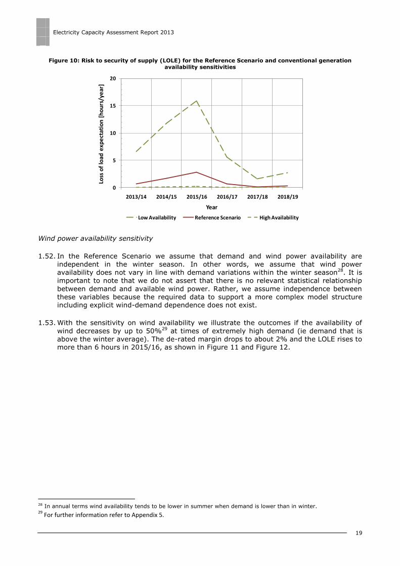
1.51. Figure 9 and Figure 10 present the de-rated capacity margins and risks measures for
these sensitivities. As shown in the figures, the de-rated margin for the low availability
sensitivity is less than 1% in 2015/16 with a LOLE of around 16 hours per year, while in
the high availability sensitivity the de-rated margin is about 7% and the LOLE is close to
zero for the same year.
Figure 9: De-rated capacity margins for the Reference Scenario and conventional generation availability sensitivities
25 The proportion of other variable sources of generation such as solar is very limited in the current GB market. 26 We use the mean plus and minus one standard deviation to find the variations for these sensitivities. 27 We do not use this assumption in the Reference Scenario as we do not have evidence in this sense.
0%
5%
10%
15%
2013/14 2014/15 2015/16 2016/17 2017/18 2018/19
De
-rat
ed
cap
acit
y m
argi
n [
%]
Year
Low Availability Reference Scenario High Availability
Electricity Capacity Assessment Report 2013
19
Figure 10: Risk to security of supply (LOLE) for the Reference Scenario and conventional generation availability sensitivities
Wind power availability sensitivity
1.52. In the Reference Scenario we assume that demand and wind power availability are
independent in the winter season. In other words, we assume that wind power
availability does not vary in line with demand variations within the winter season28. It is
important to note that we do not assert that there is no relevant statistical relationship
between demand and available wind power. Rather, we assume independence between
these variables because the required data to support a more complex model structure including explicit wind-demand dependence does not exist.
1.53. With the sensitivity on wind availability we illustrate the outcomes if the availability of
wind decreases by up to 50%29 at times of extremely high demand (ie demand that is
above the winter average). The de-rated margin drops to about 2% and the LOLE rises to more than 6 hours in 2015/16, as shown in Figure 11 and Figure 12.
28 In annual terms wind availability tends to be lower in summer when demand is lower than in winter. 29
For further information refer to Appendix 5.
0
5
10
15
20
2013/14 2014/15 2015/16 2016/17 2017/18 2018/19
Loss
of
load
exp
ect
atio
n [
ho
urs
/ye
ar]
Year
Low Availability Reference Scenario High Availability

Electricity Capacity Assessment Report 2013
20
Figure 11: De-rated capacity margins for the Reference Scenario and wind generation availability sensitivities
Figure 12: Risk to security of supply (LOLE) for the Reference Scenario and wind generation availability sensitivities
Potential impacts on customers
1.54. As noted earlier, most supply deficits in the GB market are not noticeable for customers
as the System Operator can manage small events using a range of mitigation actions.
These include voltage control, requesting maximum generation from plant or requesting emergency services from the interconnectors.
1.55. If all mitigation actions were exhausted and demand was still not met, the System
Operator would proceed with the controlled disconnection of customers by asking the
Distribution Network Operators (DNOs) to disconnect load. The DNOs would start
shedding the largest loads first, which would likely be industrial users and then go down
the list of electricity consumers at the time. In addition, information would be provided to
0%
5%
10%
15%
2013/14 2014/15 2015/16 2016/17 2017/18 2018/19
De
-rat
ed
cap
acit
y m
argi
n [
%]
Year
Reference Scenario Low Wind
0
2
4
6
8
10
2013/14 2014/15 2015/16 2016/17 2017/18 2018/19
Loss
of
load
exp
ect
atio
n [
ho
urs
/ye
ar]
Year
Reference Scenario Low Wind

Electricity Capacity Assessment Report 2013
21
the market to reduce demand (rather than disconnect). This would most likely start by
appealing for industrial and commercial customers to reduce demand then moving to the
next stage by asking customers in general to reduce demand and to avoid turning on
appliances at peak times. This process is covered by stages of emergency actions which are detailed in the Grid Code30.
1.56. We estimate the probability of controlled disconnections of customers, including both
non-domestic and domestic, to increase from around 1 in 47 years in 2013/14 to around 1 in 12 years in 2015/16 before falling to 1 in 112 years in 2018/19.
1.57. The probability of controlled disconnections of customers follows the same trend as the
LOLE, though it is by definition smaller as only some shortfalls would lead to controlled
disconnections. The sensitivity presenting the highest probability of controlled
disconnections is the low conventional generation availability sensitivity, which peaks at around 1 in 2 years in 2015/16.
Structure of the report
1.58. The Electricity Capacity Assessment Report 2013 is structured as follows:
Chapter 2 presents a brief description of the methodology used for our analysis.
Chapter 3 describes the assumptions for the Reference Scenario and sensitivities.
Chapter 4 presents the results in terms of de-rated margins and risk measures and potential implications for customers.
Appendix 1 further expands our analyses introducing specific studies and
sensitivities. Appendix 2 compares our estimations of the risk measures from last
year‟s Electricity Capacity Assessment report with those from this report. Appendix
3 lays out a detailed description of the model. Appendix 4 introduces an analysis of
the contribution of interconnector flows to security of supply. Appendix 5 details the
numerical results behind the figures presented throughout this report in table
format. Appendix 6 provides a glossary of terms used.
30 Note that the explanation presented in this document is for illustration purposes only and it is not intended to
provide precise information. This process is accurately documented in the appropriate provisions of the Grid Code, as described in OC6 (Demand Control), OC7 (Operational Liaison) and BC1 (Balancing Code).

Electricity Capacity Assessment Report 2013
22
2. Methodology
2.1. This chapter describes the methodology used for this report. In particular, we explain the
modelling approach and indicators used to assess the risk to electricity security of supply in GB. A detailed description of the modelling approach can be found in Appendix 3.
2.2. Like the 2012 report, the 2013 report uses a combination of a probabilistic approach and
sensitivity analysis. We use a probabilistic approach to assess the uncertainty related to
short-term variations in demand and available conventional generation due to outages
and wind generation. This is combined with sensitivity analysis to assess the uncertainty
related to the evolution of electricity demand and supply due to investment and
retirement decisions (ie mothballing, closures) and interconnector flows, among others.
2.3. The Reference Scenario represents a view of the future outlook for security of supply
based on the information currently available to us. It is presented to facilitate comparison
with the various sensitivities. Our analysis sets out an updated assessment of the risks to
electricity security of supply in Great Britain over the next six winters (ie from 2013/14
to 2018/19).
2.4. The methodology was designed by Ofgem and National Grid and the probabilistic model
was developed by National Grid in close collaboration with Ofgem. The methodology was
consulted upon with industry31 and academics. The probabilistic model was validated by LCP Consulting.
Modelling Approach
High level approach and outputs
2.5. The Capacity Assessment model is a probabilistic model that analyses capacity adequacy
in GB. Under the current characteristics of the GB market, any problems related to
generation adequacy are likely to materialise during the winter season32. Therefore, our
model uses a distribution of demand during winter season. Times of extremely high
demand that may cause emergency situations are represented in the tails of the demand distribution.
2.6. Our model is a time-collapsed model; this means that it calculates the probability of
demand exceeding available supply (supply deficit) at a randomly chosen half-hour from
the winter period. Due to the physical characteristics of electricity systems, a supply
deficit does not necessarily mean that customers will be disconnected but it means that
the SO will need to intervene to try and avoid disconnections. Only large supply deficits
lead to disconnections in the GB system. We estimate the possible frequency and
duration of any shortfalls to provide an indication of the risk of controlled disconnections of customers.
2.7. Figure 13 below presents a schematic representation of the model. The inputs for
investment and retirement decisions (new build, closures, mothballing) are based on
National Grid‟s Future Energy Scenarios33 amended to reflect Ofgem‟s views, mainly with
31 The methodology was consulted with industry and academics in 2011 and 2012. The consultation documents, corresponding responses and decision documents can be found in http://www.ofgem.gov.uk. 32 This has been demonstrated with the analysis of the summer period included in Appendix 1. 33 The Future Energy Scenarios are developed annually by National Grid to illustrate potential scenarios of the future development of the GB electricity and gas sectors. For further information refer to:
http://www.nationalgrid.com/uk/Gas/OperationalInfo/TBE/Future+Energy+Scenarios

Electricity Capacity Assessment Report 2013
23
regards to the impact of policy uncertainty. The inputs on interconnector flows are based
on Ofgem‟s assumptions while expected demand, available conventional capacity (de-
rating factors), and the characteristics of wind farms are based on historical data and
analysis from National Grid. The wind speeds are based on the Modern Era Retrospective-
analysis for Research and Applications (MERRA) dataset produced by the National
Aeronautics and Space Administration (NASA).
Figure 13: Schematic representation of the modelling approach34
2.8. There are five key outputs from our modelling: two probabilistic measures of security of
supply, Loss of Load Expectation (LOLE) and Expected Energy Unserved (EEU); the
frequency and duration of expected outages, the Equivalent Firm Capacity (EFC) of wind power and the de-rated capacity margin:
LOLE: the mean number of hours per year in which supply does not meet demand in the absence of intervention from the System Operator.
EEU: the mean amount of electricity demand that is not met in a year. EEU
combines both the likelihood and the potential size of any supply shortfall.
Frequency and duration of expected outages: an illustration of the results of
the probabilistic risk measures in terms of tangible impacts for electricity customers.
This is based on judgements around how the electricity system would operate at a
time when supply does not meet demand, and the order and size of mitigation
actions taken by the System Operator. It is therefore not as accurate as the LOLE
and EEU but it allows us to provide a view of the probability of experiencing controlled disconnections of customers.
EFC: the quantity of firm capacity (ie always available) that can be replaced by a
certain volume of wind generation to give the same level of security of supply, as
measured by LOLE. This measure is used to calculate the average contribution of
wind power to the de-rated margin. It varies with the proportion of wind power in the system.
De-rated capacity margin: the average excess of available generation capacity
over peak demand, expressed in percentage terms. Available generation capacity
takes into account the contribution of installed capacity at peak demand by
34 The green boxes represent inputs based on historical/factual data, the blue boxes represent inputs based on Ofgem‟s assumptions, the red boxes represent calculation modules and the yellow boxes are the outputs of the modelling.
Demand
(including DSR)
Wind
Generation
Conventional
Generation
Wind speeds
Wind farms
Installed
Conventional
Availability
Risk
Calculation
EEU
LOLE
Frequency
and duration
Voltage
Reduction
Interconnectors
EFC
De-rated
Margin
Emergency
Services
Closures,
new build, mothballed
Max
Generation

Electricity Capacity Assessment Report 2013
24
adjusting it by the appropriate de-rating (or availability) factors which take into account the fact that plant are sometimes unavailable due to outages.
2.9. LOLE is not a measure of the expected number of hours per year in which customers may
be disconnected. We define LOLE to indicate the number of hours in which the system may need to respond to tight conditions.
2.10. For a given level of LOLE and EEU, results may come from a large number of small
events where demand exceeds supply in principle but it can be managed by National Grid
through a set of mitigation actions available to them as System Operator35. The results
may also come from a small number of large events (eg the supply deficit is more than 2
to 3GW36) where controlled disconnections cannot be avoided. Conversely, given the
characteristics of the GB system, any shortfall is more likely to take the form of a large number of small events that would not have a direct impact on customers.
2.11. LOLE serves to take account of the impact of rising levels of variable generation.
However, it may not reflect any potential improvements37 in the capacity of the system
to cope with more variability before any disconnections. We do not expect these improvements to have a significant impact in the market in the next six winters.
Quantifying LOLE and EEU
2.12. To calculate the LOLE and EEU, in the six winter modelling period, the model constructs
probability distributions of winter demand38, wind power and available conventional
generation. The LOLE and EEU are calculated by combining (ie through convolution39) the
three distributions; this represents the main risk calculation. The outcome of the
convolution is a distribution of margins (ie the difference between supply and demand)
for each winter in the modelling period. The LOLE and EEU are then estimated from the part of the distribution for which supply is lower than demand.
2.13. The distribution of winter demand is based on rescaled historical demand data and
demand growth projections provided by National Grid. The distribution of wind power is
based on wind speed data which is used to estimate the corresponding levels of wind generation associated with the projected installed wind capacity.
2.14. The distribution of available conventional generation is derived from installed capacities
combined with a de-rating factor. The de-rating factors are derived from the analysis of
the historical availability performance of the different generating technologies, at times of
winter peak period. The winter peak period is defined here as the days in winter where
35 The System Operator can implement mitigation actions to maintain the system when available supply is insufficient to meet demand. These include voltage control, maximum generation instruction and emergency services from the interconnectors. 36 This varies with the specific conditions of the market at the time of the outage, including the flows over the interconnectors at the time. 37 One potential improvement would be for example further penetration of frequency management through automated appliances. For further information refer to:
http://www.ofgem.gov.uk/Pages/MoreInformation.aspx?file=20130430_Creating%20the%20right%20environment%20for%20demand-side%20response.pdf&refer=Markets/sm/strategy/dsr 38 Winter demand is based on Average Cold Spell (ACS) demand. This reflects the combination of weather elements (ie temperature, illumination and wind) that give rise to a level of peak demand within a financial year that has a 50% chance of being exceeded as a result of weather variations alone. 39 Convolution is the mathematical operation of obtaining the distribution of the sum of two independent random variables from their individual distributions.

Electricity Capacity Assessment Report 2013
25
demand is greater than the median40 of daily demands from October to March, in every year41.
2.15. We assume that interconnectors will respond to price differentials in the future after the
implementation of Market Coupling in 2013. However, we cannot model future price
differentials between GB and interconnected markets with sufficient precision due to all
the uncertainty surrounding the evolution of the North-Western European electricity
markets. Consequently, we use informed assumptions based on the analysis presented in
Appendix 4 where we considered the structure of the GB and interconnected markets, historical price differentials and the security of supply outlook in these markets.
2.16. The uncertainties surrounding the evolution of both supply and demand are significant.
Hence, our report includes sensitivity analysis to account for a range of possible views42.
Each sensitivity assumes a change in one variable43 from the Reference Scenario, with all
other assumptions being held constant. The purpose of this is to assess the impact of the
uncertainty related to each variable in isolation, on the risk measures. Our report is not
using scenarios (ie a combination of changes in several variables to reflect alternative
worlds or different futures), as this would not allow us to isolate the impact of each variable on the risk measures.
Frequency and duration of outages
2.17. LOLE is not a measure of the expected number of hours per year in which customers may
be disconnected. To illustrate the potential impact on customers, we also estimate the
frequency and duration of outages of a given severity when mitigation actions available
to the System Operator have been exhausted. These actions cover demand reduction (eg
voltage control) and potential supply increases. The frequency and duration estimates
help us to illustrate possible impacts on customers of supply shortfalls (ie the average
frequency of controlled disconnections of customers given the volume of demand). The tools available to the System Operator are discussed below.
Voltage reduction: For small events, both in terms of energy and duration, the SO
can manage the system by instructing voltage control. This is subsequently applied
by the DNOs. This action involves reducing the voltage level and hence the level of
consumption. The SO estimates the maximum level of demand reduction that can be achieved through this measure to be 500MW44.
Maximum generation: The maximum generation action is a service where the SO
instructs generators to generate at the maximum possible output. This involves
operating a generator above 100% of its rated output45. The amount of available
extra capacity through the maximum generation is estimated at around 250MW by the SO.
40 The median is the value that separates the higher half of the data set from the lower half. By using only periods where demand is higher than the median we are ensuring that we only use the higher half of the data set which represent periods of high demand during the winter. 41 For further information refer to Chapter 3. 42 For further information refer to Chapter 3. 43 For example, in the demand sensitivities we have developed, the only variable changing is demand. 44 This is based on National Grid‟s operational experience. Section OC6.5.3. of the Grid Code outlines the obligations for demand control for the DNOs. 45 This mode of operation causes significant wear and tear to the generator and as a result this measure can only be applied rarely.

Electricity Capacity Assessment Report 2013
26
Emergency services from interconnectors46: Emergency services from
interconnectors are used as a last resort solution before initiating controlled
disconnections of GB customers. In the event of a supply shortfall, after all other
measures have been exhausted, the SO can request assistance from the SOs of the
interconnected markets. Specifically, the SO-SO agreements in place enable the SO
to request the reduction of exports from GB or the increase of imports from the
neighbouring markets . The available volume through emergency services from
interconnectors depends on the level of imports and exports prior to requesting emergency services.
2.18. Figure 14 illustrates the mitigation actions available to the SO and their potential sequence.
Figure 14: Schematic representation of mitigation actions
Interpreting risks to security of supply
2.19. The probabilistic measures of security of supply presented in this report are often
misinterpreted. LOLE is the expected number of hours per year in which supply does not
meet demand. This does not however mean that customers will be disconnected or that
there will be blackouts for that number of hours a year. Most of the time, when available
supply is not high enough to meet demand, National Grid may implement mitigation
actions to solve the problem without disconnecting any customers. However, the system
should be planned to avoid the use of mitigation actions and that is why we measure
LOLE ahead of any mitigation actions being used.
2.20. LOLE does not necessarily mean disconnections but they do remain a possibility. If the
difference between available supply and demand is so large that the mitigation actions
are not enough to meet demand then some customers have to be disconnected – this is
the controlled disconnections step in Figure 14 above. In this case the SO will disconnect
industrial demand before household demand.
2.21. The model output numbers presented here refer to a loss of load of any kind. This could
be the sum of several small events (controlled through mitigation actions) or a single
large event. As a consequence of the mitigation actions available, the total period of
disconnections for a customer will be lower than the value of LOLE. Even when a single large event occurs, part of the problem is solved with mitigation actions.
2.22. As an illustration of the impacts on customers, we also present in the report the 1-in-n
years probability of controlled disconnections metric. This illustrates the (noticeable)
consequences of the reported LOLE and EEU on customers specifically (ie after the
mitigation actions have been used). The 1-in-n years estimate is an approximation only
as it is very difficult to perform a precise calculation. We present it in order to help
46 For further information refer to:
http://www.nationalgrid.com/uk/Electricity/Balancing/services/balanceserv/systemsecurity/sotoso/
Demand ≥ Supply
Voltage reduction
Maximum generation
Emergency services from
interconnectors
Controlled disconnections
up to 500 [MW] up to 250 [MW]up to 2,000 [MW]
(depending on magnitude and direction of flows)
1–in–n yearsLOLE

Electricity Capacity Assessment Report 2013
27
understand the potential situations that could arise but it should not be used for planning purposes.
2.23. The 1-in-n figure refers to the controlled disconnection of both industrial and household
demand. The process to implement controlled disconnection of customers is as follows. If
all mitigation actions were exhausted and the required System Margin was still not met,
the System Operator would ask the Distribution Network Operators and Non-Embedded
Customers and Suppliers to proceed with controlled demand reduction. National Grid will
endeavour to achieve demand reduction in a manner that is equitable to all users, in
order to avoid or reduce unacceptable operating conditions on any part of the GB Transmission System.
2.24. Each DNO ensures it can provide a 20% reduction of its total system demand in four
incremental stages (between 4% and 6%), which can be achieved at all times, with or
without prior warning, and within 5 minutes of receipt of an instruction from the System
Operator. The reduction of a further 20% (40% in total) can be achieved following issue of the appropriate GB System Warning by National Grid within agreed timescales47.
2.25. We are not able to calculate how many households (if any) would be disconnected in the
event of a large outage – as this will depend on a number of factors, including the level of industrial demand at the time.
2.26. The LOLE and EEU estimates are just an indication of risk. There is considerable
uncertainty around the main variables in the calculation (eg demand, the behaviour of
interconnectors etc.). Therefore, we run sensitivities to show the range of possible
outcomes depending on these uncertainties. For example, the Reference Scenario and
sensitivities make different assumptions on the level and direction of interconnector flows with Ireland and mainland Europe.
2.27. The impact of interconnectors on LOLE is different from their impact on the 1-in-n
probability of controlled disconnections. Our assumption is that, regardless of the
assumptions on the level and direction of flows during normal winter conditions in the
Reference Scenario and sensitivities (which have a direct impact on LOLE), we can almost
always count on interconnectors to reduce the probability of controlled disconnections.
For illustration, the probability of requiring voltage control would be higher if GB were
exporting electricity to France compared to a situation where GB were importing
electricity from France. However, the GB System Operator will be able to request
assistance from the interconnectors by reducing exports before disconnecting any GB
customers.
2.28. The inclusion of exports to Ireland and/or mainland Europe in the Reference Scenario or
sensitivities does not mean that GB would be exporting electricity abroad while
disconnecting customers in GB. As explained above, the SO makes use of mitigation
actions before resorting to controlled disconnections. One of these actions is the
provision of emergency services from interconnectors. Depending on the agreements in
place (and the sensitivity assumptions) this would mean that exports could be reduced in
an emergency situation and/or that imports from other markets could be called upon to
alleviate any gap between supply and demand. As such, none of the sensitivities in our report calculate the probability of disconnection estimates while GB is a net exporter.
47 This process is covered in the appropriate provisions of the Grid Code, as described in OC6 (Demand Control), OC7 (Operational Liaison) and BC1 (Balancing Code).

Electricity Capacity Assessment Report 2013
28
Quantifying and interpreting de-rated capacity margins
2.29. Finally, we calculate the de-rated capacity margins for each winter. The de-rated margin
represents the average excess of generation capacity over peak demand and is
expressed in percentage terms. This “typical” available capacity is the sum of the
average available conventional capacity and the Equivalent Firm Capacity (EFC48) of wind
generation. The EFC is the quantity of firm capacity (ie always available) that can be
replaced by a certain volume of wind generation to give the same level of security of supply, as measured by LOLE.
2.30. De-rated margins are not good indicators of security of supply because they do not
reflect the amount of variability associated with them, which can differ significantly
depending on the generation mix. By way of illustration, two systems with the same de-
rated margin may have significantly different levels of risks depending on the proportion
of variable generation capacity (eg wind power) in each system. Although the average
availability of wind power is taken into account by de-rating the capacity, there is a much
wider variation around this average (depending on wind conditions) than there is for conventional generation.
2.31. Comparing de-rated margins over time does not give an accurate picture in terms of
risks as the proportion of wind power in the GB system has increased considerably in
recent years and is expected to continue doing so. All else remaining equal, de-rated
margins will need to increase steadily over time in order to achieve the same level of
security of supply. Nonetheless, de-rated margins are a familiar and intuitive indication of
trends in the short to medium term.
2.32. Generally, when the variations in the generation mix are not extensive (as is the case
during the period evaluated in this report) the LOLE and EEU tend to increase when the
de-rated margins decrease and vice versa. However, the effects are not symmetrical.
Importantly, a change in the de-rated margins when they are low has a larger impact on
the risks (eg LOLE and EEU) than a change of the same magnitude in the de-rated
margins when they are high. This emphasises the importance of exploring plausible lower
de-rated margins through sensitivities to get a better sense of the risks to security of supply in GB in the coming years.
48 For further information on the calculation of EFC and the rationale for using this measure to find the de-rated capacity of wind power refer to Appendix 3.

Electricity Capacity Assessment Report 2013
29
3. Assumptions
3.1. This chapter describes the model input assumptions. It is split into three sections. We
first present the assumptions on the supply side, followed by the assumptions on the
demand-side. Finally we present the assumptions around interconnector flows. Each section describes the assumptions for the Reference Scenario and relevant sensitivities.
3.2. The Reference Scenario builds on National Grid‟s Gone Green 2013 scenario from its
forthcoming Future Energy Scenarios. We have made adjustments to National Grid‟s
supply-side assumptions to reflect our own views on the closure, mothballing and new
build decisions of generators, and on interconnector flows. Each sensitivity is designed to
vary only one variable and hold all other variables constant. The purpose of this is to
assess the uncertainty related to an individual variable, and its impact on the risks to
security of supply.
3.3. An important factor for our supply, demand and interconnector flows assumptions is the
energy policy in place. We have only modelled policies that are already in place or for
which a decision has been taken. Therefore our assumptions do not reflect the impact of
the potential implementation of a Capacity Market or cash-out reform. No additional
Energy Market Reform (EMR) policies are taken into account in our analysis. We assume that Market Coupling49 is implemented from the winter of 2013/14.
Supply
3.4. This section presents assumptions on the supply side. We have followed a similar
approach to the 2012 report. More specifically, the assumptions for the Reference
Scenario build on National Grid‟s Gone Green 2013 scenario, amended for the latest
public information on recent and future capacity changes. The assumptions are also
amended to reflect Ofgem‟s views regarding the evolution of installed capacity due to the
uncertainty in future market conditions and policy.
3.5. Decisions on whether power stations close, return to service or are built depend on
companies‟ specific commercial and financial position, the outlook for energy prices as
well as the energy policy environment. It is very difficult to form a firm view on these
decisions. We have therefore developed sensitivities to explore the effect of these key
uncertainties on our risk measures.
3.6. We use the most up-to-date market information at the time of publication relating to the
capacities of generators. The assumptions for the Reference Scenario and sensitivities are presented in the next section.
Reference Scenario
3.7. Since the publication of Ofgem‟s 2012 report, a number of plant have announced their
permanent closure or mothballing. Some of these plant closures and mothballing
decisions were expected while others were not anticipated. Total installed capacity is
49 “Market Coupling is the method by which Day Ahead energy prices and volumes for each local market are calculated by gathering all Day Ahead bids and offers (collectively termed orders in the network code) in the different local markets in order to match them at European level on a marginal pricing basis”, ENTSO-E, Network code on Capacity Allocation & Congestion Management (CACM). This definition could be extended to other electricity products (eg intra-day prices). For further information refer to:
https://www.entsoe.eu/fileadmin/user_upload/_library/consultations/Network_Code_CACM/120323_NetworkCodeConsultation_FINAL.pdf

Electricity Capacity Assessment Report 2013
30
expected to be around 77.9GW in the winter of 2013/14 (down from 79.5GW in our 2012
report), falling steadily to 76.8GW by 2015/16 (down from 79.3GW in our 2012 report),
before increasing to 83.6GW in 2018/19. Figure 15 presents the installed capacity by
technology in GB over the next six winters.
Figure 15: Installed capacity by generation technology type in the Reference Scenario
3.8. The generation mix changes over time. Fossil fuel capacity (around 6.3GW) is expected
to be replaced by new variable wind generation and biomass plant (around 12.4GW) in
the timeframe of our analysis. In particular, older coal and oil plant will close due to the
requirements of European environmental legislation, while some coal plant are expected
to convert to biomass. Some nuclear capacity is also expected to retire over the period. CCGT capacity is expected to vary during the period of analysis.
3.9. Figure 16 presents the change in installed capacity for each technology type in each
winter of analysis.
Figure 16: Changes in installed capacity by generation technology type in the Reference Scenario
0
20
40
60
80
100
2012/13 2013/14 2014/15 2015/16 2016/17 2017/18 2018/19
Cap
acit
y [G
W]
Year
Wind - Offshore
Wind - Onshore
Tidal
Biomass
Hydro
Pumped storage
Nuclear
Oil
GT
CCGT
Coal
Reference Scenario 2012
-6
-4
-2
0
2
4
6
2013/14 2014/15 2015/16 2016/17 2017/18 2018/19
Cap
acit
y [G
W]
Year
Additions Wind Offshore
Additions Wind Onshore
Additions Biomass
Additions CCGT
Closures Biomass
Closures Nuclear
Closures Oil
Closures GT
Closures CCGT
Closures Coal

Electricity Capacity Assessment Report 2013
31
3.10. The changes in the installed capacity due to closures, mothballs and new-builds, by technology type are discussed in turn below.
Closures
3.11. A number of plant are expected to close over the analysis period. These closures are
mainly driven by the Large Combustion Plant Directive (LCPD) that restricts the operation of coal and oil plant, and plant reaching the end of their technical lifetime.
3.12. Under the LCPD directive, fossil-fuelled generating plant must choose to either reduce
their emissions or opt-out of the Directive50. Coal plant that opt-out are restricted to
operating for 20,000 hours51 between 1 January 2008 and 31 December 2015, by which
time they must close52. A total of 12GW of coal and oil plant in GB opted-out of the
Directive will have to close by the end of December 2015. Two coal plant, with a
combined capacity of 2GW, have also opted-out of the LCPD, but have converted to
generate from biomass. This would result in a reduction of their available capacity of around 0.5GW53.
3.13. The bulk of LCPD closures have already been realised, with over 7GW having shut down
permanently by the end of winter 2012/13 and an extra 0.7GW of biomass plant
expected to close before winter 2013/14. Additionally, we expect 1GW of coal plant to
close at the end of 2013/14 and 0.7GW of biomass plant to close at the end of 2014/15. Only 1.1GW of oil plant are expected to remain operational until the end of 2015.
3.14. Opted-in LCPD coal capacity is expected to decrease over the course of the period,
mainly due to plant conversions from coal to biomass. In particular, around 2.5GW of
opted-in coal plant are expected to convert to biomass by 2016/17. This is due to the
profitability of coal generation decreasing with the implementation of the Carbon Floor
Price (CPF)54, while biomass conversion is supported by governmental policy through the
Renewable Obligation55. In addition 0.3GW of opted-in LCPD coal capacity is scheduled to close permanently by 2014/15.
3.15. The Industrial Emissions Directive (IED)56 will place restrictions on the operation of some
existing coal and older CCGT stations post 2016/201757. This creates uncertainty in the
market as generators have until January 2014 to decide whether to opt-in or opt-out of
the Directive. We assume that the IED does not affect the supply situation in the
timeframe of our analysis.
50 The LCPD aims to reduce the emission levels of sulphur dioxide (SO2) and nitrogen oxides (NOx) from large combustion plants, including power plants, across Europe. For more information see:
http://www.defra.gov.uk/industrial-emissions/eu-international/lcpd 51 Opted-out LCPD oil plant are restricted to 10,000 hours of operation in the same period. 52 The LCPD required coal and oil plant to fit pollution abatement equipment to comply with the emission limits set by the Directive. However, it gave coal and oil plant the option to opt-out of this provision, thus restricting their operation times. 53 As plant convert from coal to biomass their capacity is reduced due to the lower heat content of biomass compared to coal. 54 For further information refer to:
http://www.hmrc.gov.uk/climate-change-levy/carbon-pf.htm 55 For further information refer to:
https://www.gov.uk/government/uploads/system/uploads/attachment_data/file/42842/3235-consultation-ro-banding.pdf 56 For further information refer to:
http://www.defra.gov.uk/industrial-emissions/eu-international/industrial-emissions-directive 57 Under the IED, coal and old CCGT plants can either fit emission reduction equipment to comply with the requirements, or take one of two derogations available. The hours based restriction (Limited Lifetime Obligation, LLO) and emissions based restriction (Transitional National Plan) will both limit the load factors of these stations.

Electricity Capacity Assessment Report 2013
32
3.16. Approximately 500MW of nuclear capacity is scheduled to close before winter 2014/15.
The two nuclear plant that were due to reach the end of their technical lifetimes within
the period of analysis have been granted lifetime extensions that put their closures
beyond 2018/1958. No further nuclear plant closures are assumed in the Reference Scenario.
3.17. It is expected that some older CCGT plant will come offline after the mid-decade, as they
reach the end of their technical lifetime. We assume that 0.3GW of CCGT plant will close permanently in 2016/17 and 2017/18 combined, with another 2.2GW closing in 2018/19.
Mothballing of plant
3.18. One of the most difficult issues to form a firm view on relates to mothballing of plant.
Since the publication of our 2012 report, the number of CCGT plant mothballed has
increased in the GB system. Generators have cited low profitability for gas generation as the main driver for recent mothballing decisions.
3.19. We assume around 1.5GW of mothballed plant in winter 2013/14. An additional 0.8GW of
gas plant are expected to mothball before winter 2014/15. We assume that around
0.5GW of mothballed plant will be brought back on the system in 2015/16 and an additional 0.7GW in 2016/17 as margins get tighter.
New-builds
3.20. Decisions on whether power stations are built depend on companies‟ specific commercial
and financial decisions. During the analysis period, we expect the installed capacity of
wind and biomass to increase, mainly driven by Government support policies and some
new CCGT plant becoming operational.
3.21. Installed capacity of wind has been growing for more than a decade59. It is expected that
wind capacity will continue to grow over the next six winters, driven mainly by support
policies and decreasing costs for the technology. Wind capacity is assumed to increase
from 10.2GW in 2013/14 to 20.1GW in 2018/19 with the installation of Round 2 to 3
offshore wind farms, and the further deployment of onshore wind, both transmission connected and embedded.
3.22. Our assumptions on CCGT capacity include just under 1GW of new build, which is due to
start construction. We assume that half of it will come online in winter 2016/17 and the rest in 2017/18.
3.23. As coal plant convert to biomass, we expect the installed capacity of biomass to increase,
with a simultaneous decrease in coal capacity. While plant conversions are expected to
lead to an additional 2.4GW of biomass plant between 2014/15 and 2016/17, this
represents a net reduction in total capacity as the capacity of the converted plant is lower than the coal plant it replaces.
3.24. In addition, we assume that 0.7GW of biomass plant (converted LCPD opt-out plant) is
relicensed and becomes operational from 2014/15. A further 0.1GW of dedicated biomass plant are assumed to come online in 2017/18.
58 Two of the Advanced Gas Cooled Reactors that were scheduled to retire in 2016 have received a seven year lifetime extension. 59 For further information refer to: “Wind: State of the Industry 2012”, by renewableUK (information relevant to the entire UK, ie GB and Northern Ireland).

Electricity Capacity Assessment Report 2013
33
Conventional and wind generation availabilities
3.25. In order to estimate the available generation capacity we need to de-rate the installed
capacity by the corresponding de-rating factors that represent the availability of different
generation technology types.
3.26. Estimating de-rating factors is a complex task given that it is difficult to differentiate
between technical (unexpected) outages, and capacity withdrawals as a result of market
conditions (strategic outages) from the historical data, creating potential bias in the results.
3.27. Conventional generation availabilities are derived from the analysis of the historical
availability performance of the different generating technologies during the winter peak
period. We defined winter peak period as the days in winter where demand is greater than the median of daily demands from October to March, in every year (2005 to 2012).
3.28. By considering the winter peak period, we are reflecting in our de-rating factors the
potential for plant to increase their availability at times of high demand, and hence
increase prices,. In the Reference Scenario the de-rating factors per technology type are
estimated as their average availability over the past seven winter estimates (ie from 2005 to 2012).
3.29. An important input assumption on the supply side is the contribution of wind generators
to security of supply. Wind power availability is more variable than the availability of
conventional generation due to the variable nature of wind speeds. Therefore, we use a
different approach to calculate the contribution of wind to security of supply by
calculating the Equivalent Firm Capacity (EFC)60 for each winter and sensitivity. The EFC
shows the contribution of wind generation to security of supply by taking into account the
margin changes in the GB system. The EFC values are in the range of 17% – 24% of the
installed wind capacity for the Reference Scenario; depending on the winter under study
(the lower values correspond to the later winters of the analysis period where the
proportion of wind power in the generation mix is larger). Appendix 3 presents a detailed description of the calculation method for EFC.
3.30. Table 1 shows the availability (ie de-rating factors) of generators per technology type for the Reference Scenario.
Table 1: Generator de-rating factors per technology type
Fuel type Availability [%]
Coal / Biomass 88%
Gas CCGT / Gas CHP 85%
OCGT 92%
Oil 82%
Nuclear 81%
Hydro 84%
Pumped Storage 96%
Wind (EFC) 17% – 24%
60 The EFC is the quantity of firm capacity (ie always available) that can be replaced by a certain volume of wind generation to give the same level of security of supply, as measured by LOLE.

Electricity Capacity Assessment Report 2013
34
Sensitivities
3.31. We have used sensitivities to explore the effects of uncertainties in the key assumptions
on the supply side. Below we present sensitivities around the Reference Scenario relating
to the potential evolution of supply, the available wind resource at times of extreme demand, and the de-rating factors of conventional generators.
Supply
3.32. High supply sensitivity: we assume that market signals for CCGT plant improve and
their profitability increases. In addition, there is an upside risk that generators will invest
in new plant or not mothball existing plant despite uncertainty in the market. Therefore
we assume that no additional CCGT is mothballed, some is brought back on the system, and the construction of new CCGT plant accelerates.
3.33. In the high supply sensitivity we assume that an additional 1.4GW of CCGT is available in
2013/14 increasing to 2.3GW in 2014/15. The amount of additional CCGT plant assumed
to be available on the system decreases from 2014/15, to reflect the decrease in the
availability of mothballed plant in that year. It is also assumed that 0.5GW of new CCGT
becomes operational a winter earlier than in the Reference Scenario, in 2016/17, and an
additional 2GW of new CCGT comes online for winter 2018/19. In the winter of 2014/15,
0.5GW of additional nuclear plant is assumed to be granted extension of its period of operation and therefore we consider it being available.
3.34. Low supply sensitivity: we assume the profitability of gas and oil plant remains
unfavourable, leading to additional plant being mothballed or shutting down. In addition,
there is a risk that uncertainty and lack of confidence around energy policies results in a lack of investment in new plant and additional plant being mothballed.
3.35. In low supply sensitivity, we assume that no new CCGT gets built within the timeframe of
the analysis, reducing CCGT capacity by around 0.9GW from winter 2017/18 with respect
to the Reference Scenario. We assume an additional 0.7GW of CCGT is mothballed in
2016/17. In addition, we assume approximately 0.4GW of oil plant shut down in 2013/14 and an additional 0.7GW of biomass plant are unavailable from 2014/15.
3.36. Figure 17 presents the changes in installed capacity by generation technology type for the high and low supply sensitivities compared to the Reference Scenario.
Figure 17: Installed capacity changes for the high and low supply sensitivities with respect to the Reference Scenario
-4
-2
0
2
4
2013/14 2014/15 2015/16 2016/17 2017/18 2018/19
Cap
acit
y [G
W]
Year
Biomass (Low Supply)
Oil (Low Supply)
CCGT (Low Supply)
Nuclear (High Supply)
CCGT (High Supply)

Electricity Capacity Assessment Report 2013
35
Conventional generation availability
3.37. De-rating factors are derived from the analysis of the historical availability performance
of the different conventional technologies at times of winter peak demand, from 2005 to
2012. In the Reference Scenario the availability per technology type is defined as the mean availability over the past seven winter estimates.
3.38. As the availability of conventional power plants shows a significant amount of variation
on a year-to-year basis, we have developed two sensitivities to account for potentially
higher or lower availability per technology type than in the Reference Scenario. The low
conventional availability sensitivity reflects the potential of reduced plant availability, eg
due to the ageing of the generation fleet or more variable patterns of utilisation of
conventional plant61. The high conventional availability sensitivity illustrates the case
where generators increase their availability at times of peak demand to profit from higher
prices. The low and high bounds are estimated by statistical analysis of the plant availability over the past seven winters62.
3.39. Table 2 details the availability of the generators per technology type for the low and high conventional availability sensitivities.
Table 2: Generator availability per technology type
Fuel type Availability [%]
Low High
Coal / Biomass 86% 90%
Gas CCGT / Gas CHP 81% 89%
OCGT 87% 97%
Oil 75% 89%
Nuclear 76% 86%
Hydro 78% 90%
Pumped Storage 93% 99%
Wind generation availability
3.40. There is not yet sufficient data for wind generation during winter in GB to enable us to
understand the relationship, if any, between wind availability and high demand63.
Therefore, in the Reference Scenario we make the assumption that there is no
relationship between these variables at the time of high demand. This means that the
distribution of wind power and winter demand are estimated separately, although the distribution of wind is based on historical wind speeds over winter.
3.41. However, there is a widespread belief that the wind stops blowing when there is a severe
cold spell, resulting in lower wind availability at the time of high demand for electricity.
Figure 18 presents the relationship between the wind load factor and daily peak demand
observed from 2005 to 2012. Figure 18 illustrates that the available wind appears to
decrease as daily peak demand increases. However, there is insufficient data to find this
trend statistically significant and so we have taken the possibility into account via the wind-demand sensitivity.
61 This could be driven by the need to operate plant flexibly as more variable wind generation becomes operational. 62 The low and high bounds are estimated as the mean availability ± one standard deviation, based on the annual availabilities per technology type over the past seven winters. 63 From the security of supply perspective, we are mainly interested in the available wind resource at times of high demand.

Electricity Capacity Assessment Report 2013
36
Figure 18: Wind load factor at times of daily peak demand
3.42. For the wind generation availability sensitivity we assume that wind availability decreases
at time of high demand. In particular this sensitivity assumes a reduction in the available
wind resource for demand levels higher than 92% of the ACS peak demand. The
maximum reduction is assumed to be 50% for demand levels higher than 102% of ACS peak demand64.
Demand
3.43. Electricity demand assumptions for the Reference Scenario are taken from the Gone
Green 2013 scenario assumptions produced by National Grid for its Future Energy
Scenarios. National Grid expect economic growth, energy efficiency and demand
management to be the main variables driving changes in demand over the period of our
analysis.
3.44. Demand is very difficult to predict, especially during an economic downturn and with
uncertain weather patterns. For example, demand could be significantly higher than
expected due to severe winter conditions. In addition, it is also very difficult to anticipate
the impact of energy efficiency policies on energy use. We have thus developed sensitivities around the potential evolution of electricity demand.
3.45. The demand used in our analysis is the ACS peak demand, which is demand adjusted for
the effect of weather variations. It reflects demand at winter peak under average
weather conditions. The basis for this is the demand as seen by National Grid on the
transmission network net of embedded generation65 and demand-side response66 to which the contribution of embedded wind at peak67 is added.
64 For further information refer to Appendix 3. 65 Embedded generation is generation connected to the distribution network. This consists of a range of technologies including for example small scale Combined Heat and Power, generation from landfill gas, and biomass. The electricity generated by such schemes is typically used in the local system rather than being transported across the UK, and hence manifests as a reduction in demand as seen by National Grid.
0%
20%
40%
60%
80%
100%
90% 92% 94% 96% 98% 100% 102%
Win
d lo
ad fa
ctor
Daily peak demand (as percentage of ACS peak)

Electricity Capacity Assessment Report 2013
37
Reference Scenario
3.46. Demand for electricity has been declining since 2008, primarily as a result of the
economic downturn and the implementation of energy efficiency measures. Figure 19
depicts the evolution of the historical ACS peak demand from 2005 together with the
National Grid‟s Gone Green 2013 projected ACS peak demand up to the winter of 2018/19 inclusive.
Figure 19: Historic and projected ACS peak demand
Economic growth
3.47. National Grid‟s Gone Green scenario is based on an axiom of moderate economic growth,
benchmarked against external economic forecasts68. The Gone Green 2013 scenario
assumes that the economy will rebound slowly and GDP growth rates will reach 2.3% by
the end of the analysis period69. This growth is expected to drive demand higher in the
industrial sector, where the contribution of the sector at ACS peak demand grows by
0.5GW between 2013/14 and 2018/19. This is partly offset by a reduction in demand
from the commercial sector. National Grid in their Gone Green 2013 scenario project
demand in the commercial sector to drop by 0.4GW in the same period, driven mainly by a reduction in non-manufacturing productivity.
3.48. Table 3 presents the forecast for GDP growth assumed in National Grid‟s Gone Green 2013 scenario.
66 Demand-side response refers to an active, short term reduction in electricity consumption as seen by National Grid either through shifting it to another period or replacing transmission connected generation with embedded generation, or simply not using electricity at that time. 67 The contribution of wind is added back to demand as we are modelling wind, transmission connected and embedded generation, explicitly in our model. The contribution of embedded wind at peak is based on National Grid‟s assessment. 68 GDP growth forecasts are provided to National Grid by Experian Business Strategies. 69 The OBR expects a similar GDP growth in the first couple of winters (eg 1.8% in winter 2014/15) and higher rates in the later winters (eg 2.8% in 2017/18). For further information refer to:
http://cdn.hm-treasury.gov.uk/budget2013_complete.pdf
45
50
55
60
65
2005/06 2006/07 2007/08 2008/09 2009/10 2010/11 2011/12 2012/13 2013/14 2014/15 2015/16 2016/17 2017/18 2018/19
AC
S p
eak
de
man
d [
GW
]
Year
Historic Final Gone Green 2012
Reference Scenario 2012 (Provisional Gone Green 2012) Reference Scenario 2013 (Final Gone Green 2013)
Slow Progression 2013

Electricity Capacity Assessment Report 2013
38
Table 3: Forecast of GDP growth
GDP growth
2011/12 2012/13 2013/14 2014/15 2015/16 2016/17 2017/18 2018/19
GDP used
for Reference Scenario (2011/12 = 100)
100 99.9 100.7 102.3 104.2 106.3 108.6 111.1
% change
year-on-year
n/a -0.1% +0.8% +1.6% +1.9% +2.0% +2.2% +2.3%
Note: (+) Increase; (-) Decrease.
Energy efficiency
3.49. Energy efficiency has been a flagship policy area across the European Union over recent
years. The GB government is implementing a series of policies to drive higher energy efficiency in both the domestic and non-domestic sectors70.
3.50. National Grid, in their Gone Green 2013 scenario, project energy efficiency measures to
drive demand down across all sectors and particularly in the domestic sector. They
project the increased penetration of energy efficient appliances and lighting technologies
to result in a reduction of overall energy demand, and subsequently ACS peak demand,
in the domestic sector. Table 4 shows the variation in ACS peak demand due to energy
efficiency measures in the domestic sector with respect to the winter of 2013/14.
National Grid project energy efficiency policies to have a minimal impact on demand in the industrial and commercial sectors.
Table 4: Variation in ACS peak demand due to energy efficiency measures in the domestic sector
Variable
[GW] 2013/14 2014/15 2015/16 2016/17 2017/18 2018/19
Variation in ACS peak demand 0 -0.4 -0.7 -1.3 -1.9 -2.4
Note: (+) Increase; (-) Decrease.
Demand-side response (DSR)
3.51. DSR refers to customers responding to a signal by changing the amount of energy they
consume from the grid at a particular time71. These signals could include prices,
incentives, information or contracts. From a Capacity Assessment perspective we are
interested in the level of electricity DSR during periods of high demand. During these
periods, DSR may result in demand reduction; however, DSR may result in an increase in demand at non-peak times when a temporary peak reduction is compensated for.
3.52. Demand in our analysis is treated net of demand reduction due to DSR. National Grid
currently estimates that around 1GW of DSR is available from the non-domestic sector
70 For example, the Green Deal and Energy Company Obligation (ECO) target mainly energy efficiency in the domestic sector, and the Carbon Reduction Commitment (CRC) Energy Efficiency Scheme targets energy efficiency in the non-domestic sector. 71 For further information refer to the Ofgem consultation “Creating the right environment for demand-side response”.
http://www.ofgem.gov.uk/Markets/sm/strategy/dsr/Documents1/20130430_Creating%20the%20right%20environment%20for%20demand-side%20response.pdf

Electricity Capacity Assessment Report 2013
39
through triad avoidance72. National Grid project DSR in the non-domestic sector to grow over the course of the analysis period from 1.2GW in 2013/14 to 2GW in 2018/19.
3.53. In the domestic sector, it is expected that smart metering, through the effects of time-of
use tariffs73, will lead to greater amounts of DSR. In National Grid‟s Gone Green 2013
scenario, DSR in the domestic sector grows from negligible levels in 2013/14 to 0.4GW in 2018/19.
3.54. Table 5 summarises the assumed impact of DSR participation on ACS peak demand over the next six winters.
Table 5: Variation in ACS peak demand due to DSR programmes
Variation in ACS peak demand
[GW] 2013/14 2014/15 2015/16 2016/17 2017/18 2018/19
Non-domestic sector
(triad avoidance) -0.2 -0.3 -0.5 -0.7 -0.8 -1
Domestic sector
(smart metering) 0 -0.1 -0.1 -0.2 -0.3 -0.4
Note: (+) Increase; (-) Decrease.
Other drivers
3.55. National Grid project the penetration of new technologies to result in an increase in ACS
peak demand. However, ACS peak demand decreases due to the net effect of all drivers.
Specifically, heat pumps74 and electric vehicles are assumed to contribute an additional 0.7GW at ACS peak demand by 2018/19.
3.56. In addition, National Grid project further deployment of embedded generation
technologies to have a downward effect on ACS peak demand. These technologies, and
especially small-scale CHP generation, are assumed to reduce ACS peak demand by 0.5GW by 2018/19.
Largest infeed loss reserve
3.57. National Grid reserves power to maintain the integrity of the network in the event of the
loss of the largest generator (the largest infeed loss)75. Its importance is such that
National Grid would curtail demand before using this reserve. We therefore consider it on the demand-side in our analysis.
3.58. National Grid currently holds around 0.7GW of capacity to meet the largest infeed loss
requirements and expects that no projects are likely to have a higher requirement before
72 Triad refers to the three half-hourly periods of highest demand during a winter season. National Grid determines the charges to suppliers, and subsequently customers, for the use of the transmission network based on average of their triad demand. Hence, customers have an incentive to reduce their demand during the triad periods. Demand reduction at the time of triad is called triad avoidance. 73 Time of use tariffs refers to the variable pricing of electricity consumption based on varying costs of generation. 74 Heat pumps are assumed to replace economy 7 electric storage heating, which is generally not operating at times of peak demand. As a result, heat pumps result in a net increase of demand at times of peak demand. 75 Currently the National Electricity Transmission System Security Quality of Supply Standards, which is approved by Ofgem, limits the largest infeed loss reserve to approximately 1.3GW. The limit is scheduled to increase to 1.8GW in April 2014. For further information refer to:
http://www.nationalgrid.com/uk/Electricity/Codes/gbsqsscode/. National Grid is currently working with the DNOs to better understand the risk of a large infeed loss causing the consequential loss of distributed generation. The findings of this work should inform further analysis of the reserve to secure the system against the largest infeed loss.
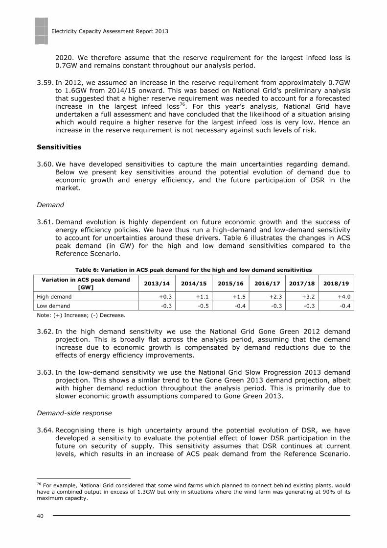
Electricity Capacity Assessment Report 2013
40
2020. We therefore assume that the reserve requirement for the largest infeed loss is 0.7GW and remains constant throughout our analysis period.
3.59. In 2012, we assumed an increase in the reserve requirement from approximately 0.7GW
to 1.6GW from 2014/15 onward. This was based on National Grid‟s preliminary analysis
that suggested that a higher reserve requirement was needed to account for a forecasted
increase in the largest infeed loss76. For this year‟s analysis, National Grid have
undertaken a full assessment and have concluded that the likelihood of a situation arising
which would require a higher reserve for the largest infeed loss is very low. Hence an
increase in the reserve requirement is not necessary against such levels of risk.
Sensitivities
3.60. We have developed sensitivities to capture the main uncertainties regarding demand.
Below we present key sensitivities around the potential evolution of demand due to
economic growth and energy efficiency, and the future participation of DSR in the market.
Demand
3.61. Demand evolution is highly dependent on future economic growth and the success of
energy efficiency policies. We have thus run a high-demand and low-demand sensitivity
to account for uncertainties around these drivers. Table 6 illustrates the changes in ACS
peak demand (in GW) for the high and low demand sensitivities compared to the Reference Scenario.
Table 6: Variation in ACS peak demand for the high and low demand sensitivities
Variation in ACS peak demand
[GW] 2013/14 2014/15 2015/16 2016/17 2017/18 2018/19
High demand +0.3 +1.1 +1.5 +2.3 +3.2 +4.0
Low demand -0.3 -0.5 -0.4 -0.3 -0.3 -0.4
Note: (+) Increase; (-) Decrease.
3.62. In the high demand sensitivity we use the National Grid Gone Green 2012 demand
projection. This is broadly flat across the analysis period, assuming that the demand
increase due to economic growth is compensated by demand reductions due to the effects of energy efficiency improvements.
3.63. In the low-demand sensitivity we use the National Grid Slow Progression 2013 demand
projection. This shows a similar trend to the Gone Green 2013 demand projection, albeit
with higher demand reduction throughout the analysis period. This is primarily due to
slower economic growth assumptions compared to Gone Green 2013.
Demand-side response
3.64. Recognising there is high uncertainty around the potential evolution of DSR, we have
developed a sensitivity to evaluate the potential effect of lower DSR participation in the
future on security of supply. This sensitivity assumes that DSR continues at current
levels, which results in an increase of ACS peak demand from the Reference Scenario.
76 For example, National Grid considered that some wind farms which planned to connect behind existing plants, would have a combined output in excess of 1.3GW but only in situations where the wind farm was generating at 90% of its maximum capacity.
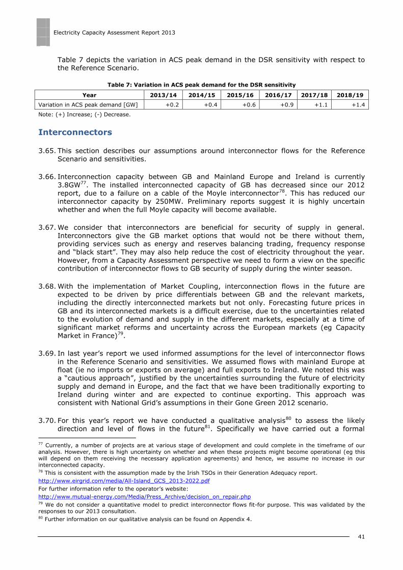
Electricity Capacity Assessment Report 2013
41
Table 7 depicts the variation in ACS peak demand in the DSR sensitivity with respect to the Reference Scenario.
Table 7: Variation in ACS peak demand for the DSR sensitivity
Year 2013/14 2014/15 2015/16 2016/17 2017/18 2018/19
Variation in ACS peak demand [GW] +0.2 +0.4 +0.6 +0.9 +1.1 +1.4
Note: (+) Increase; (-) Decrease.
Interconnectors
3.65. This section describes our assumptions around interconnector flows for the Reference
Scenario and sensitivities.
3.66. Interconnection capacity between GB and Mainland Europe and Ireland is currently
3.8GW77. The installed interconnected capacity of GB has decreased since our 2012
report, due to a failure on a cable of the Moyle interconnector78. This has reduced our
interconnector capacity by 250MW. Preliminary reports suggest it is highly uncertain
whether and when the full Moyle capacity will become available.
3.67. We consider that interconnectors are beneficial for security of supply in general.
Interconnectors give the GB market options that would not be there without them,
providing services such as energy and reserves balancing trading, frequency response
and “black start”. They may also help reduce the cost of electricity throughout the year.
However, from a Capacity Assessment perspective we need to form a view on the specific contribution of interconnector flows to GB security of supply during the winter season.
3.68. With the implementation of Market Coupling, interconnection flows in the future are
expected to be driven by price differentials between GB and the relevant markets,
including the directly interconnected markets but not only. Forecasting future prices in
GB and its interconnected markets is a difficult exercise, due to the uncertainties related
to the evolution of demand and supply in the different markets, especially at a time of
significant market reforms and uncertainty across the European markets (eg Capacity
Market in France)79.
3.69. In last year‟s report we used informed assumptions for the level of interconnector flows
in the Reference Scenario and sensitivities. We assumed flows with mainland Europe at
float (ie no imports or exports on average) and full exports to Ireland. We noted this was
a “cautious approach”, justified by the uncertainties surrounding the future of electricity
supply and demand in Europe, and the fact that we have been traditionally exporting to
Ireland during winter and are expected to continue exporting. This approach was consistent with National Grid‟s assumptions in their Gone Green 2012 scenario.
3.70. For this year‟s report we have conducted a qualitative analysis80 to assess the likely
direction and level of flows in the future81. Specifically we have carried out a formal
77 Currently, a number of projects are at various stage of development and could complete in the timeframe of our analysis. However, there is high uncertainty on whether and when these projects might become operational (eg this will depend on them receiving the necessary application agreements) and hence, we assume no increase in our interconnected capacity. 78 This is consistent with the assumption made by the Irish TSOs in their Generation Adequacy report.
http://www.eirgrid.com/media/All-Island_GCS_2013-2022.pdf
For further information refer to the operator‟s website:
http://www.mutual-energy.com/Media/Press_Archive/decision_on_repair.php 79 We do not consider a quantitative model to predict interconnector flows fit-for purpose. This was validated by the responses to our 2013 consultation. 80 Further information on our qualitative analysis can be found on Appendix 4.

Electricity Capacity Assessment Report 2013
42
analysis of the structure of and interactions between GB and its interconnected markets
to identify possible outcomes. Actual interconnector flows will be determined by price
differentials in the future. Hence, these results should be taken as indicators of possible
outcomes instead of precise forecasts and are complemented with plausible sensitivities.
3.71. We conclude that we can only anticipate with a significant degree of certainty that GB will
export electricity to Ireland in the next six winters, as we expect prices in Ireland to be
higher than in GB. This is supported by the current level of price differentials between the
two markets, their similarities and market outlook. With regards to the interconnectors
with mainland Europe at periods of low margins, on average:
We may or may not import electricity from the Netherlands depending, among
others, on the situation in the German and Belgium markets, and potential mothballing and closure decisions across Europe;
We may or may not import from or export to France depending on the evolution of
the market in France and its interconnected markets, including Germany and
Belgium82.
3.72. The qualitative analysis consists of two elements: structural analysis and historical analysis. Both are described below.
Structural analysis
3.73. GB is not the only European Market expecting decreasing capacity margins in the next six
winters. France and Ireland are facing similar challenges. The situation in the
Netherlands is different as the Dutch power sector is going through a period of important
investment in new plant. This means, the Netherlands is expected to be a net exporter of
electricity over the course of the analysis period. However, the Netherlands is
interconnected with Germany and Belgium and the direction of their export flows will be determined by the price differentials between Germany, Belgium, and GB.
3.74. In addition, there are no evident complementarities83 between GB and its interconnected
markets as we have very similar patterns of demand and supply availability. Historically,
the evolution of margins in these interconnected markets has been positively correlated84
which means that when margins are low in one market they tend to be low in other markets.
3.75. Furthermore, demand, which is the main driver for changes in the level of margins, is
also correlated between GB and its interconnected markets. Therefore, it is possible to
experience periods of tight margins at the same time at both ends of all GB interconnectors.
3.76. We do not expect the availability of conventional generation to be correlated between GB
and its interconnected markets in the future. As the penetration of wind increases in GB
and the relevant markets the correlation of available generation might change in the
81 A qualitative analysis was supported by the response to our 2013 Capacity Assessment consultation. 82 France, Germany and Belgium are considering the implementation of Capacity Markets to ensure security of supply in the future. 83 For example, in hydro-based South American markets the rainy season in the Northern hemisphere coincides with the dry season in the Southern hemisphere resulting in opposite cycles of generation availability which are the main drivers of margins in these interconnected markets. 84 Correlation is a measure of dependence between two variables. A positive correlation indicates that as one variable increase so too does the other, whilst a negative correlation indicates that as one increases the other decreases. A correlation of zero means there is no dependence between the variables.

Electricity Capacity Assessment Report 2013
43
future. This will depend on the levels and proportion of installed wind in the different
markets and the location of the installed wind. Subsequently, any correlation of the wind
resource in GB and the relevant markets could have an impact on the correlation of available generation.
Historical Analysis
3.77. We analysed how interconnector flows have responded in the past to changes in the main
GB system parameters: demand, capacity margins, availability of conventional
generation, availability of wind power, and prices. No consistent pattern of response has
been identified to any of these parameters. This increases the difficulty in assessing future interconnector flows.
3.78. With the implementation of Market Coupling from winter 2013/14 we can broadly expect
flows to follow the direction of higher prices85. Our analysis of historical price differentials
demonstrates that only Ireland and GB have shown a consistent pattern, with GB prices
being consistently and significantly lower than prices in Ireland in the past. The
differences with other markets are variable in direction and magnitude and are expected
to change in the future given market changes and reforms currently under development
in the different markets (eg EMR in Great Britain, Capacity Market in France, nuclear
phase-out in Germany and Switzerland, and the implementation of Market Coupling for North-West Europe).
Reference Scenario
3.79. Based on these two analyses, the Reference Scenario takes a cautious approach to interconnector flows similarly to the 2012 analysis. In particular, we assume:
Full exports to Ireland (750MW), based on historical flows and expected price
differentials between GB and Ireland;
Interconnector flows with mainland Europe are at float, ie not importing or exporting
on average, due to high levels of uncertainty with regards to future price differentials between GB and the markets of mainland Europe.
3.80. Table 8 details our assumptions for the interconnector flows (in MW) during winter peak periods in the Reference Scenario.
Table 8: Interconnector flow assumptions (in MW) at winter peak periods for the Reference Scenario
Name To 2013/14 2014/15 2015/16 2016/17 2017/18 2018/19
Moyle SEM (NW) -250 -250 -250 -250 -250 -250
East-West SEM (RoI) -500 -500 -500 -500 -500 -500
IFA France 0 0 0 0 0 0
BritNed Netherlands 0 0 0 0 0 0
Note: (+) Great Britain Imports; (-) Great Britain Exports.
85 Market Coupling is expected to be implemented across North-West Europe in 2013. The implementation will initially be across the day-ahead markets. The target is to extend Market Coupling in the intra-day markets. It is uncertain when the implementation of Market Coupling across intra-day markets will be in place.

Electricity Capacity Assessment Report 2013
44
Sensitivities
3.81. To assess the uncertainty surrounding the interconnector flows we complement the
analysis with sensitivities to illustrate what would happen if flows were higher or lower than expected.
3.82. Therefore, we have developed a range of interconnector sensitivities which make
different assumptions on imports/exports with mainland Europe at peak times. These are
described below and presented in Table 9.
The full imports sensitivity assumes 3GW interconnection imports with France and
the Netherlands across the entire analysis period compared to the Reference
Scenario (full exports of 750MW to Ireland assumed). We do not present a full
exports sensitivity as we consider the possibility to export at full capacity during
peak demand highly unlikely given this would result in negative de-rated margins in
GB. We expect prices to reflect this and improved interconnector responsiveness, as a result of the implementation of Market Coupling in the future;
Half import/export sensitivities assume ± 1.5GW interconnection flows with France
and the Netherlands compared to the Reference Scenario (full exports of 750MW to Ireland assumed).
Table 9: Interconnector flow assumptions (in GW) at winter peak periods for sensitivities
Sensitivity 2013/14 2014/15 2015/16 2016/17 2017/18 2018/19
Full imports +3.0 +3.0 +3.0 +3.0 +3.0 +3.0
Half imports +1.5 +1.5 +1.5 +1.5 +1.5 +1.5
Half exports -1.5 -1.5 -1.5 -1.5 -1.5 -1.5
Note: (+) Great Britain Imports; (-) Great Britain Exports.
No net interconnector flows
3.83. We also include a sensitivity which excludes interconnector flows. In this sensitivity the
de-rated margins and risk measures are estimated based only on domestic demand and
the availability of domestic generation. This approach may be helpful to DECC when
making decisions to procure extra capacity through a Capacity Market due to the high
levels of uncertainty surrounding the assessment of future interconnector flows. In
addition, including exports in the demand projections when calculating how much
capacity to procure through policy interventions would mean supporting investment to secure demand abroad as well as demand in GB.
3.84. The Energy-only Market will continue to operate in parallel to any policy intervention to
procure extra capacity. Therefore, excluding exports to Ireland from the calculations of
how much capacity to procure on top of what would be delivered by the energy only
market alone does not imply that exports will not take place. Exports will continue to
respond to the energy-only market rules and will take place under regular conditions if
prices in GB are lower than those in Ireland.

Electricity Capacity Assessment Report 2013
45
4. Results
4.1. In this chapter we present the results of our assessment on the levels of risk to security
of supply and of the associated de-rated capacity margins for the GB electricity sector over the next six winters.
4.2. We use two well established probabilistic measures to quantify the risks to security of supply:
Loss of Load Expectation (LOLE): is the mean number of hours per year in which
supply does not meet demand in the absence of intervention from the System
Operator.
Expected Energy Unserved (EEU): is the mean amount of electricity demand that is
not met in a year. EEU combines both the likelihood and the potential size of any supply shortfall.
4.3. Moreover, to illustrate the impacts on customers of the risk measures in our assessment
(LOLE and EEU) we have also calculated the frequency of occurrence of supply shortfall
events large enough that they might lead to controlled customer disconnections. We do
this by calculating the frequency of a range of supply shortfall events that vary in
magnitude from 0-10MW to 2,750MW+. We explain that only in the case of supply
shortfalls greater in magnitude than 2,750MW is there a risk of controlled customer
disconnections.
4.4. This chapter is structured as follows. We start with a description of the risks to security of
supply (LOLE, EEU and the risk of customer disconnections) in the Reference Scenario.
We follow this with an examination of the results in each of our major sensitivities
(demand, supply, interconnector flows and both conventional plant and wind power
availabilities). The chapter concludes by looking at the associated de-rated capacity margins in the Reference Scenario and each of our major sensitivities.
Measures of risk and impact on customers
Reference Scenario
4.5. Figure 20 and Figure 21 present the estimated LOLE and EEU for the GB electricity sector from winter 2013/14 to winter 2018/19 for the Reference Scenario.
4.6. Figure 20 shows that the LOLE for next winter 2013/14 is estimated at 0.7 hours per
year. Broadly this means that we estimate the expected number of hours that electricity
demand is higher than available supply (a supply shortfall) in winter 2013/14 to be
around 0.7 hours per year. Note that this is from a total of 8,760 hours in a one year
period86. The LOLE is then expected to increase towards winter 2015/16 when it reaches
a level of 2.9 hours per year. This is largely driven by the closure of power plant over this
period87. The LOLE is then estimated to decrease to 0.1 hours per year in winter
2017/18. This improvement is driven by the entry of new capacity, (mostly wind and gas
CCGTs) and a decline in electricity demand. At the end of our period of analysis, we
86 While our analysis is carried out over the six month period that includes winter, we present the LOLE in hours per year as we have analysed the summer months in our summer sensitivity (see Appendix 1) and observe that they do not present a security of supply risk in GB and so do not contribute to our assessment of LOLE. 87 For comparison a LOLE of 2.9 hours per year is within the reliability standards used by France, Ireland and Belgium.

Electricity Capacity Assessment Report 2013
46
observe the estimated LOLE rising marginally in winter 2018/19, when it is expected to be 0.3 hours per year.
Figure 20: Loss of load expectation for the Reference Scenario
Figure 21: Expected energy unserved for the Reference Scenario
4.7. The EEU in Figure 21 follows a similar trend to the LOLE over the next six winters. For
winter 2013/14, the EEU is expected to be 659MWh. This means that we estimate the
total volume of electricity demand that cannot be met by available supply during winter
2013/14 to be 659MWh. The estimated EEU then rises in the following two winters to
reach approximately 3,070MWh by 2015/16. As with the LOLE, the estimated EEU falls in
the following two winters to reach a low of 106MWh in 2017/18. It increases again slightly in the final year of our analysis.
0
1
2
3
4
5
2013/14 2014/15 2015/16 2016/17 2017/18 2018/19
Loss
of
load
exp
ect
atio
n [
ho
urs
/ye
ar]
Year
0
1,000
2,000
3,000
4,000
5,000
2013/14 2014/15 2015/16 2016/17 2017/18 2018/19
Exp
ect
ed
en
erg
y u
nse
rve
d [
MW
h]
Year

Electricity Capacity Assessment Report 2013
47
Impact on customers
4.8. As discussed in Chapter 2, a positive value for the risk measures of LOLE and EEU does
not necessarily mean disconnections for customers, although they do remain a
possibility. This is because for a reasonably wide range of supply shortfalls, the GB SO
can employ mitigation actions that prevent the immediate disconnection of supply to
customers. Only after the SO has exhausted its available actions will customers be at risk
of disconnection. Specifically, the range of mitigation actions available to the SO are: (i)
voltage reduction; (ii) maximum generation; and (iii) emergency services from interconnectors. A detailed description of mitigations actions is provided in Chapter 2.
4.9. The impacts of these actions are generally not perceptible to electricity customers and
they can be used in parallel. Nevertheless, the SO is likely to use mitigation actions as a
last resort measure as it results in the economically inefficient operation of the electricity system and costs to the SO.
4.10. Table 10 presents supply shortfall events of increasing magnitude and aligns them with
the mitigating strategy that the SO may employ in response to them. The table shows
that the SO can manage a volume of supply shortfall in the range of 0 – 2,750MW
through a combination of voltage reduction, maximum generation and emergency
services. However, events larger than 2,750MW would probably exceed the mitigation
actions available and could result in controlled disconnections of electricity customers.
We stress that controlled disconnections would involve the largest industrial customers
first and would ensure that domestic households are protected for as long as possible as described in Chapter 2.
Table 10: Mitigation actions
Supply shortfall event
[MW] Mitigation action
0 – 10 No impact
10 – 500 Voltage reduction
500 – 750 Voltage reduction and maximum generation
750 – 2,750 Voltage reduction, maximum generation and emergency services
2,750 + Controlled disconnections
4.11. We use the information above to illustrate the potential impacts on customers of the risk
measures in our assessment (LOLE and EEU). To do this we estimate the frequency of
occurrence of supply shortfall events large enough that they might lead to controlled
customer disconnections. Table 11 presents our estimates for illustration purposes. It
shows the frequency of occurrence of increasingly large supply shortfall events for the
Reference Scenario. We would expect only those supply shortfalls on the bottom row of the table (corresponding to 2,750MW+) to risk customer disconnections.
Table 11: Frequency of supply shortfalls
Supply shortfall event
[MW]
Frequency [1 in n years]
2013/14 2014/15 2015/16 2016/17 2017/18 2018/19
0 – 10 1-in-0.10 1-in-0.04 1-in-0.03 1-in-0.1 1-in-0.5 1-in-0.2
10 – 500 1-in-0.5 1-in-0.2 1-in-0.1 1-in-0.5 1-in-3 1-in-1
500 – 750 1-in-23 1-in-10 1-in-6 1-in-24 1-in-126 1-in-55
750 – 2,750 1-in-12 1-in-5 1-in-3 1-in-12 1-in-65 1-in-28
2,750 + 1-in-47 1-in-19 1-in-12 1-in-49 1-in-256 1-in-112

Electricity Capacity Assessment Report 2013
48
4.12. Table 11 shows that the estimated frequency of supply shortfalls events of all sizes
increases over the period of analysis from winter 2013/14 to winter 2015/16. This is
consistent with the significant increases observed in LOLE and EEU for the same period.
We note, however, that the estimated frequency of the largest supply shortfalls (ie those
large enough to risk customer disconnections at 2,750MW+) is very low in winter
2013/14 at approximately 1-in-47 years, but rises to 1-in-12 years in winter 2015/16. In
the following winter, the estimated frequency of 2,750MW+ supply shortfalls declines
significantly to 1-in-49 years and further again in winter 2017/18 to 1-in-256 years. As
with the LOLE and EEU, there is a small increase in the estimated frequency of the largest supply shortfall events in winter 2018/19.
Sensitivities
4.13. We use sensitivities to investigate the impact on our risk measures of uncertainty in key
input assumptions. We have run sensitivities on our assumptions on demand, supply,
interconnector flows and both conventional plant and wind power availabilities. Each
sensitivity is designed to vary only one variable and hold all other variables constant. A detailed description behind the development of the sensitivities is presented in Chapter 3.
Supply
4.14. The level of future GB electricity supply is driven by the decisions of private companies to
close, mothball or invest in new power plants. The supply sensitivities explore the impact
on our risk measures of uncertainties surrounding these decisions.
4.15. As set out in Chapter 3, the low supply sensitivity assumes that no new plant are built
over the period of the analysis. In addition, we assume that approximately 1,200MW of
biomass and LCPD opted-out oil plant will be unavailable in winter 2014/15. An additional
700MW of CCGT is assumed mothballed from winter 2016/17 onwards. In contrast, the
high supply sensitivity assumes that some mothballed CCGT plant return to the market
and new CCGT plant are built towards the end of the analysis period. This means that in
the high supply sensitivity an additional 1,400MW of CCGT is available throughout the
period of the analysis compared to the Reference Scenario. This figure is higher
(2,300MW) in winter 2014/15 and (2,500MW) in winter 2018/19. The first rise is due to
more mothballed CCGT being available for suppliers to bring back on line and the second
rise is due to new CCGT build. The high supply sensitivity also assumes 500MW of
additional available nuclear plant in winter 2014/15.
4.16. Figure 22 and Figure 23 show the estimated LOLE and EEU for the low and high supply sensitivities over the next six winters, together with the Reference Scenario.
4.17. The figures show that the trend of the low and high sensitivities remains broadly similar
to the Reference Scenario throughout the period of analysis. It also shows that the high
supply sensitivity results in a far lower LOLE and EEU than the low demand sensitivity.
This is because the supply sensitivities are more symmetric around the Reference
Scenario than the demand sensitivities. Even so, the results indicate that with around
1,500 to 2,500MW of additional capacity available throughout the period of the analysis,
the estimated measures of risk fall to very low levels. For example, in winter 2015/16 the
LOLE is estimated to be 0.7 hours per year and the EEU is 620MWh.
4.18. In contrast, the low supply sensitivity highlights the impact on the risks to security of
supply of having around 500 to 2,500MW less capacity available throughout the period of
the analysis. In the low supply sensitivity, the maximum values of the estimated LOLE
and EEU rise to 4.8 hours and to 5,480MWh, respectively, both in winter 2015/16.

Electricity Capacity Assessment Report 2013
49
Figure 22: Loss of load expectation for the Reference Scenario and supply sensitivities
Figure 23: Expected energy unserved for the Reference Scenario and supply sensitivities
Conventional generation availability
4.19. In the Reference Scenario, we derive the availability of conventional power plants from
their average availabilities observed over the seven year period 2005 to 2012. As the
availability of conventional power plants shows a significant amount of variation on a
year-to-year basis, we have developed two sensitivities to explore the impact on our risk
measures of lower and higher availabilities per technology than those used in the
Reference Scenario. The availability assumptions considered for the two sensitivities are
presented in Chapter 3 and are based on a reasonable level of variation around the
Reference Scenario values88.
88 The low and high sensitivity are estimated as the average availability ± one standard deviation based on the annual availabilities per technology type over the past seven winters.
0
2
4
6
8
10
2013/14 2014/15 2015/16 2016/17 2017/18 2018/19
Loss
of
load
exp
ect
atio
n [
ho
urs
/ye
ar]
Year
Low Supply Reference Scenario High Supply
0
2,000
4,000
6,000
8,000
10,000
2013/14 2014/15 2015/16 2016/17 2017/18 2018/19
Exp
ect
ed
en
erg
y u
nse
rve
d [
MW
h]
Year
Low Supply Reference Scenario High Supply

Electricity Capacity Assessment Report 2013
50
4.20. Figure 24 and Figure 25 show the estimated LOLE and EEU for the low and high
conventional generation availability sensitivities over the next six winters, together with the Reference Scenario.
4.21. The figures indicate that reasonably small changes in conventional generation availability
have a material impact on the risk of supply shortfalls. This is most notable in 2015/16,
where the estimated LOLE ranges from 0.2 hours per year in the high availability
sensitivity to 16 hours per year in the low availability sensitivity, for the Reference
Scenario is 2.9 hours per year. The EEU also varies significantly in this year from
178MWh to 22,702MWh, in the high and low supply availability sensitivities, respectively.
Figure 24: Loss of load expectation for the Reference Scenario and conventional generation availability sensitivities
Figure 25: Expected energy unserved for the Reference Scenario and conventional generation availability sensitivities
0
5
10
15
20
2013/14 2014/15 2015/16 2016/17 2017/18 2018/19
Loss
of
load
exp
ect
atio
n [
ho
urs
/ye
ar]
Year
Low Availability Reference Scenario High Availability
0
5,000
10,000
15,000
20,000
25,000
2013/14 2014/15 2015/16 2016/17 2017/18 2018/19
Exp
ect
ed
en
erg
y u
nse
rve
d [
MW
h]
Year
Low Availability Reference Scenario High Availability

Electricity Capacity Assessment Report 2013
51
Wind generation availability
4.22. In the Reference Scenario we assume that wind output and demand are independent
variables, hence wind output is the same irrespective of the demand level. However,
there is some evidence that wind output falls during periods of severe cold weather and
consequently very high demand. To test the impact of this relationship on our risk measures, we have performed a sensitivity analysis.
4.23. In this sensitivity the quantity of wind output starts to fall when demand rises above
92% of the ACS peak demand. As demand rises further the quantity of wind generation
output declines, at a broadly constant rate, until it reaches 50% of its value in the
Reference Scenario at 102% of the ACS peak value. Appendix 3 provides further details of the approach.
4.24. Figure 26 and Figure 27 show the estimated LOLE and EEU for the lower wind generation
sensitivity over the next six winters, together with the Reference Scenario.
4.25. The figures show that lowering wind generation during periods of peak demand leads to a
significant increase in estimated LOLE and EEU, particularly in the second and third years
of our analysis. For example, in winter 2015/16, lower wind generation contributes to a
doubling in the values of the estimated risk measures: LOLE grows from 2.9 hours per
year in the Reference Scenario to 6 hours per year in the low wind generation sensitivity
and EEU is approximately 6,907MWh in the low wind generation sensitivity compared with 3,070MW in the Reference Scenario.
Figure 26: Loss of load expectation for the Reference Scenario and wind generation availability sensitivity
0
2
4
6
8
10
2013/14 2014/15 2015/16 2016/17 2017/18 2018/19
Loss
of
load
exp
ect
atio
n [
ho
urs
/ye
ar]
Year
Reference Scenario Low Wind

Electricity Capacity Assessment Report 2013
52
Figure 27: Expected energy unserved for the Reference Scenario and wind generation availability sensitivity
Demand
4.26. As set out in Chapter 3, future levels of electricity demand will depend on a range of
factors that include the speed of economic growth, the severity of the weather and the
success of energy efficiency programmes. To investigate the effects on our risk measures
of uncertainty around future levels of electricity demand, we have developed a low and a high demand sensitivity.
4.27. In our high demand sensitivity we assume higher economic growth than in the Reference
Scenario but its impact on demand is balanced by energy efficiency programmes. As a
result, the level of demand remains broadly flat across the analysis period. In the low
demand sensitivity we assume lower economic growth than in the Reference Scenario.
This reduces demand slightly with respect to the Reference Scenario levels. Importantly,
the low and high demand sensitivities are not symmetrical around the Reference
Scenario. By the end of the analysis period, the high demand sensitivity results in a
demand figure of 7.6% above the Reference Scenario, while in the low demand
sensitivity we estimate demand at -0.8% below the Reference Scenario by winter
2018/19.
4.28. Figure 28 and Figure 29 present the estimated LOLE and EEU in the high and low demand sensitivities, for the next six winters, together with the Reference Scenario.
4.29. The estimated results for the low demand sensitivity are similar to those in the Reference
Scenario, albeit with risks to security of supply being slightly lower overall. As in the
Reference Scenario, the low demand sensitivity reaches its peak in winter 2015/16. In
this winter the estimated LOLE is 2 hours per year and EEU is 2,028MWh, which compare
with Reference Scenario figures for LOLE and EEU of 2.9 hours per year and 3,070MWh,
respectively. By the end of the period the LOLE converges with the Reference Scenario figure.
4.30. The results of the high demand sensitivity are more striking. Here, the flat demand
profile over the period results in far higher results for LOLE and EEU. By winter 2015/16,
the LOLE is estimated to be 8.7 hours per year and the EEU is 11,130MWh, both around
three times higher than in the Reference Scenario. The high demand sensitivity highlights
0
2,000
4,000
6,000
8,000
10,000
2013/14 2014/15 2015/16 2016/17 2017/18 2018/19
Exp
ect
ed
en
erg
y u
nse
rve
d [
MW
h]
Year
Reference Scenario Low Wind

Electricity Capacity Assessment Report 2013
53
the importance of the level of demand to GB security of supply. It shows that if demand
does not fall over the coming years, other things being equal, the magnitude of expected
supply shortfalls (the EEU) could be over three times more severe by winter 2015/16. In
practice, a flat demand profile might result in higher electricity prices over this period and could prompt generators to bring back mothballed or invest in new plant.
Figure 28: Loss of load expectation for the Reference Scenario and demand sensitivities
Figure 29: Expected energy unserved for the Reference Scenario and demand sensitivities
Interconnectors
4.31. As discussed in Chapter 3, we have taken a cautious approach in the Reference Scenario
on the contribution of interconnectors to security of supply during periods of peak
demand. In the Reference Scenario, we assume interconnectors with mainland Europe
are at float (no import or export) and interconnectors to Ireland export 750MW
throughout the period of the analysis. The detailed description and rationale of the assumptions are presented in Chapter 3.
0
2
4
6
8
10
2013/14 2014/15 2015/16 2016/17 2017/18 2018/19
Loss
of
load
exp
ect
atio
n [
ho
urs
/ye
ar]
Year
Low Demand Reference Scenario High Demand
0
5,000
10,000
15,000
2013/14 2014/15 2015/16 2016/17 2017/18 2018/19
Exp
ect
ed
en
erg
y u
nse
rve
d [
MW
h]
Year
Low Demand Reference Scenario High Demand

Electricity Capacity Assessment Report 2013
54
4.32. The actual direction of interconnector flows in the future will be determined by the price
differential between the interconnected markets. This differential will depend on supply
and demand conditions in the interconnected markets and is likely to lead to outturn
interconnector flows that are lower or higher than those assumed in the Reference
Scenario. Our interconnector sensitivities explore the impact on our risk measures of
uncertainty around the direction and quantity of interconnector flows. We have developed
three sensitivities using different imports/exports on interconnectors with mainland
Europe with respect to the Reference Scenario. In all three we maintain the assumption of full exports to Ireland (750MW):
Full-import sensitivity: assumes an additional 3GW of imports from mainland Europe across the entire analysis period compared to the Reference Scenario.
Half-import/export sensitivities: two sensitivities that assume ±1.5GW
interconnector flows with mainland Europe compared to the Reference Scenario over
the next six winters.
4.33. Figure 30 and Figure 31 show the estimated LOLE and EEU for the three interconnector sensitivities over the next six winters, together with the Reference Scenario.
4.34. Figure 30 highlights the importance of interconnectors to GB security of supply. In both
the full and half-imports sensitivities, the values of LOLE and EEU significantly improve
compared to the Reference Scenario. For example, in winter 2015/16, the estimated
LOLE in the full imports sensitivity is 0.2 hours per year and the EEU is 117MWh. This
compares to a LOLE of 2.9 hours per year and an EEU of 3,070MWh in the Reference Scenario.
4.35. On the other hand, the half-exports sensitivity results in far higher risks to security of
supply. In the half-exports sensitivity, GB is exporting an additional 1,500MW to
mainland Europe. The impact of this is most stark in winter 2015/16, where the LOLE is
estimated to be 8.8 hours per year and the EEU is 11,139MWh. By 2018/19, the LOLE
and EEU in the half-exports case are significantly lower, but still well above the
equivalent Reference Scenario figures.
Figure 30: Loss of load expectation for the Reference Scenario and interconnector flows sensitivities
0
2
4
6
8
10
2013/14 2014/15 2015/16 2016/17 2017/18 2018/19
Loss
of
load
exp
ect
atio
n [
ho
urs
/ye
ar]
Year
Full Imports Half Imports Reference Scenario Half Exports

Electricity Capacity Assessment Report 2013
55
Figure 31: Expected energy unserved for the Reference Scenario and interconnector flows sensitivities
No net interconnector flows
4.36. We also analyse the risks to security of supply in a case where interconnector flows are
excluded (ie no net flow from mainland Europe or Ireland). The rationale for this analysis is explained in Chapter 3.
4.37. Figure 32 and Figure 33 show the estimated LOLE and the EEU for the Reference
Scenario together with the respective levels of risk for the no-net-flows sensitivity over
the next six winters.
Figure 32: Loss of load expectation for the Reference Scenario and no-net-flows sensitivity
0
5,000
10,000
15,000
2013/14 2014/15 2015/16 2016/17 2017/18 2018/19
Exp
ect
ed
en
erg
y u
nse
rve
d [
MW
h]
Year
Full Imports Half Imports Reference Scenario Half Exports
0
1
2
3
4
5
2013/14 2014/15 2015/16 2016/17 2017/18 2018/19
Loss
of
load
exp
ect
atio
n [
ho
urs
/ye
ar]
Year
Reference Scenario No Net Flows

Electricity Capacity Assessment Report 2013
56
Figure 33: Expected energy unserved for the Reference Scenario and no-net-flows sensitivity
4.38. We observe that having no net flows at peak demand periods has a significant impact on
our risk measures which are lower compared to the Reference Scenario where 750MW
are exported to Ireland. With no net flows, the GB electricity system will have a higher
capacity surplus to mitigate potential risks. The impact on the risk measures is most
notable in 2015/16, where the estimated LOLE declines from 2.9 hours per year in the
Reference Scenario to 1.5 hours per year in the no-net-flows sensitivity. Similarly, the estimated EEU decreases approximately 50% with respect to the Reference Scenario.
De-rated capacity margin
4.39. The de-rated capacity margin is commonly used by industry as an indicator of security of
supply. We note however, that the de-rated margin is not a measure of the risk of supply
shortfalls or the potential impact of those on electricity customers. As a result, it is
advised that de-rated capacity margins should not be compared across different markets
or over time in the same country if there have been significant changes in the generation portfolio.
4.40. In this section we present the estimated de-rated capacity margins in the Reference
Scenario and each one of our major sensitivities (demand, supply, interconnector flows and both conventional plant and wind power availabilities).
Reference Scenario
4.41. Figure 34 shows the estimated de-rated capacity margin for the Reference Scenario over the next six winters.
4.42. The figure shows that the estimated de-rated capacity margin declines from 6.3% in
winter 2013/14, to 3.8% in winter 2015/16 (its lowest point). This fall is driven by the
exit of power plants, in particular coal and oil plant over this period. Beyond winter
2015/16, the de-rated margin rises to a peak of 8.9% in winter 2017/18. This is driven
by National Grid‟s projected demand reductions in its Gone Green 2013 scenario and the entry of new capacity such gas, wind power and some biomass.
0
1,000
2,000
3,000
4,000
5,000
2013/14 2014/15 2015/16 2016/17 2017/18 2018/19
Exp
ect
ed
en
erg
y u
nse
rve
d [
MW
h]
Year
Reference Scenario No Net Flows

Electricity Capacity Assessment Report 2013
57
Figure 34: De-rated capacity margin for the Reference Scenario
4.43. Figure 35 compares the Reference Scenario de-rated capacity margin with the LOLE for
the next six winters.
4.44. The figure indicates a strong relationship between the de-rated capacity margin and
LOLE. Thus we observe in Figure 35 the LOLE tends to increase when the de-rated
margins decrease and vice versa. However, the effects are not symmetrical. Importantly,
a change in the de-rated margins when they are low has a larger impact on the risks (eg
LOLE and EEU) than a change of the same magnitude in the de-rated margins when they
are high. This emphasises the importance of exploring plausible lower de-rated margins
through sensitivities to get a better sense of the risks to security of supply in GB in the coming years.
Figure 35: Reference Scenario de-rated capacity margin and LOLE
0%
2%
4%
6%
8%
10%
2013/14 2014/15 2015/16 2016/17 2017/18 2018/19
De
-rat
ed
cap
acit
y m
argi
n [
%]
Year
0
1
2
3
4
5
0%
2%
4%
6%
8%
10%
2013/14 2014/15 2015/16 2016/17 2017/18 2018/19
Loss
of
load
exp
ect
atio
n [
ho
urs
/ye
ar]
De
-rat
ed
cap
acit
y m
argi
n [
%]
Year
De-rated capacity margin Loss of load expectation

Electricity Capacity Assessment Report 2013
58
Sensitivities
Supply
4.45. Figure 36 presents the estimated de-rated capacity margins for the high and low supply sensitivities over the next six winters, together with the Reference Scenario.
Figure 36: De-rated capacity margin for the Reference Scenario and supply sensitivities
4.46. The figure illustrates the impact on de-rated capacity margins of having higher or lower
levels of supply. In winter 2015/16, with around 700MW less capacity in the low supply
sensitivity compared with the Reference Scenario, the de-rated margin falls to 2.8%. In
contrast, in the same year, the high supply sensitivity gives a figure of 6.3%. The high supply sensitivity peaks at 11.7% in winter 2018/19.
Conventional generation availability
4.47. Figure 37 presents the estimated levels of de-rated capacity margins for the low and high
conventional generation availability sensitivities over the next six winters, together with the Reference Scenario.
4.48. The figure highlights the impact on the de-rated capacity margins of varying conventional
generation availability. Notably, the estimated de-rated margin varies between 0.5% and
7% in the low and high availability cases, respectively, for winter 2015/16. This
compares with 3.8% in the Reference Scenario.
0%
5%
10%
15%
2013/14 2014/15 2015/16 2016/17 2017/18 2018/19
De
-rat
ed
cap
acit
y m
argi
n [
%]
Year
Low Supply Reference Scenario High Supply
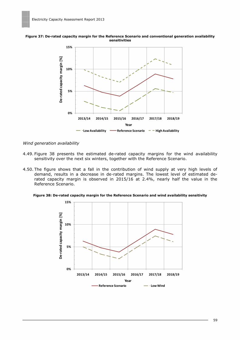
Electricity Capacity Assessment Report 2013
59
Figure 37: De-rated capacity margin for the Reference Scenario and conventional generation availability sensitivities
Wind generation availability
4.49. Figure 38 presents the estimated de-rated capacity margins for the wind availability sensitivity over the next six winters, together with the Reference Scenario.
4.50. The figure shows that a fall in the contribution of wind supply at very high levels of
demand, results in a decrease in de-rated margins. The lowest level of estimated de-
rated capacity margin is observed in 2015/16 at 2.4%, nearly half the value in the
Reference Scenario.
Figure 38: De-rated capacity margin for the Reference Scenario and wind availability sensitivity
0%
5%
10%
15%
2013/14 2014/15 2015/16 2016/17 2017/18 2018/19
De
-rat
ed
cap
acit
y m
argi
n [
%]
Year
Low Availability Reference Scenario High Availability
0%
5%
10%
15%
2013/14 2014/15 2015/16 2016/17 2017/18 2018/19
De
-rat
ed
cap
acit
y m
argi
n [
%]
Year
Reference Scenario Low Wind

Electricity Capacity Assessment Report 2013
60
Demand
4.51. Figure 39 presents the estimated de-rated capacity margins for the high and low demand sensitivities over the next six winters, together with the Reference Scenario.
Figure 39: De-rated capacity margin for the Reference Scenario and demand sensitivities
4.52. The figure shows that the low demand sensitivity only has a small effect on the de-rated
capacity margin with respect to the Reference Scenario. This is expected, given how
close the demand figures of the Reference Scenario and low demand sensitivities are.
However, the impact of the high demand sensitivity is greater. Here, the high demand
sensitivity results in de-rated margins at a lower level than in the Reference Scenario.
Notably, the estimated de-rated margin falls below 2% in winters 2015/16 and 2018/19.
Interconnectors
Figure 40: De-rated capacity margin for the Reference Scenario and interconnector flows sensitivities
0%
2%
4%
6%
8%
10%
2013/14 2014/15 2015/16 2016/17 2017/18 2018/19
De
-rat
ed
cap
acit
y m
argi
n [
%]
Year
Low Demand Reference Scenario High Demand
0%
5%
10%
15%
20%
2013/14 2014/15 2015/16 2016/17 2017/18 2018/19
De
-rat
ed
cap
acit
y m
argi
n [
%]
Year
Full Imports Half Imports Reference Scenario Half Exports

Electricity Capacity Assessment Report 2013
61
4.53. Figure 40 presents the estimated de-rated capacity margins for the three interconnector flow sensitivities over the next six winters, together with the Reference Scenario.
4.54. The figure highlights the impact that the direction of interconnector flows can have on
the estimated level of the de-rated capacity margins in GB. With full imports, in winter
2015/16, the estimated de-rated capacity margin rises to 8.9%, which is about a third
higher than the de-rated capacity margin in our high supply sensitivity (see Figure 36).
This also compares, in the same year, with 6.3% in the half-imports case and 3.8% in
the Reference Scenario. In the half-exports case the estimated de-rated capacity margin
is 1.5% in 2015/16. For all the sensitivities, the de-rated capacity margins peak in
2017/18. Where the de-rated margin for the full-imports sensitivity, is 14.5%, almost
double the value in the Reference Scenario.
No net interconnector flows
4.55. Figure 41 compares the size of the de-rated capacity margins attained under the no-net-flows sensitivity and the Reference Scenario throughout the period of analysis.
4.56. The figure shows that having no net flows (ie no net flow from mainland Europe or
Ireland) improves the de-rated capacity margin throughout the period. For the winter of
2015/16, no net flows in GB increases the estimated de-rated margin from by 3.8% in
the Reference Scenario to 5% in the no-net-flows sensitivity.
Figure 41: De-rated capacity margin for the no-net-flows sensitivity
0%
5%
10%
15%
2013/14 2014/15 2015/16 2016/17 2017/18 2018/19
De
-rat
ed
cap
acit
y m
argi
n [
%]
Year
Reference Scenario No Net Flows

Electricity Capacity Assessment Report 2013
62
Appendices
Index
Appendix Name of appendix Page number
Appendix 1 – Detailed results 63
Appendix 2 – Comparing the 2012 and 2013 reports 73
Appendix 3 – Modelling approach 77
Appendix 4 – Analysis of the contribution of interconnector flows 99
Appendix 5 – Detailed results tables 110
Appendix 6 – Glossary 116

Electricity Capacity Assessment Report 2013
63
Appendix 1 – Detailed results
1.1. This appendix contains details for additional sensitivities which are not covered in the
main part of the report. The sensitivities undertaken in the appendix are as follows:
Transmission boundary constraint
Summer season
Demand and wind confidence intervals
Demand-side response
Gas stress test
National Grid Gone Green scenario 2013
Transmission boundary constraint
1.2. Another possible cause of system risk can arise from physical limitations in certain areas
on the GB transmission network. For instance, a situation could arise where nationally
there is enough generation to supply overall demand, but in a particular region demand
cannot be met. This is because there may be insufficient transmission capacity to transfer power from the area with surplus generation to that with a generation shortfall.
1.3. According to National Grid, the Cheviot boundary, between Scotland and England, is
expected to be the most constrained transmission network link in GB over the period of
analysis. Table 12 summaries the generation and demand assumptions on either side of
the Cheviot boundary for the Reference Scenario. We represent this by the MW surplus in
ACS peak demand over installed capacity in all of England & Wales (EW) and Scotland (SC) separately. We also include the Cheviot transmission boundary capacity in MW.
Table 12: Surplus capacity in EW and SC and Cheviot boundary capacity
Variable
[MW] 2013/14 2014/15 2015/16 2016/17 2017/18 2018/19
Surplus capacity in EW over
ACS peak demand 15,418 15,553 15,080 17,133 19,834 19,693
Surplus capacity in SC over
ACS peak demand 6,980 6,525 7,156 7,992 9,480 11,521
Transmission capacity 3,300 3,300 4,300 6,400 6,400 6,400
1.4. Table 12 shows that the surplus capacities in EW and SC both follow an increasing trend
over the period. This increase is notably higher in percentage terms in Scotland than in
England and Wales, largely due to the volumes of wind generation that are estimated to
be built in Scotland. The table also indicates that the capacity of the Cheviot boundary is due to almost double from 2016/17 onwards.
1.5. Despite Table 12 showing that the surplus capacity in both EW and SC is always positive,
the physical limitations (eg limited transfer capability and availability) of the Cheviot
boundary could potentially impact our risk measures of security of supply. To test the
impact of the presence of the boundary, we have run a sensitivity that treats the GB
system as two interconnected regions, ie EW and SC. We summarise in Table 13 the

Electricity Capacity Assessment Report 2013
64
impact of the Cheviot boundary on our risk metrics LOLE and EEU. In each case, we have also presented the change in LOLE and EEU with respect to the Reference Scenario.
Table 13: Impact of the Cheviot boundary in the risk metrics
Risk metric 2013/14 2014/15 2015/16 2016/17 2017/18 2018/19
GB LOLE [hours/year] 0.7 1.7 2.9 0.7 0.1 0.3
Additional GB LOLE [hours/year] 0.0032 0.0015 0.0002 0.0000 0.0000 0.0000
GB EEU [MWh] 659 1,746 3,070 628 106 265
Additional GB EEU [MWh] 2.1016 0.9875 0.1246 0.0000 0.0000 0.0002
1.6. Table 13 shows that before the planned capacity upgrade of the Cheviot boundary in
2015/16, there would be only very small increases in our risk measures resulting from
the presence of the limited transfer capability of the Cheviot boundary. This suggests
that the Cheviot boundary is unlikely to act as a significant constraint when electricity
generated in SC is required to meet demand in EW or vice versa. Following the capacity
upgrade in 2015/16, our results suggest that the presence of the Cheviot boundary
would have no discernable impact on our risk measures. This implies that at no time
during these years the new upgraded capacity on the boundary would act as a constraint
to the flow of electricity between Scotland and England.
Summer season
1.7. The summer season in GB differs from the winter period in two key ways. The first is that
peak demand is considerably lower in summer than in winter and the second is that planned maintenance outages historically occur more often in the summer.
1.8. Table 14 compares the assumptions for the ACS winter peak demand with summer peak
demand over the next six winters in the Reference Scenario.
Table 14: ACS peak demand and summer peak demand for the Reference Scenario
Peak demand
[MW] 2013/14 2014/15 2015/16 2016/17 2017/18 2018/19
Winter 55,550 55,150 54,590 53,900 53,040 52,340
Summer 40,300 40,010 39,604 39,103 38,479 37,971
1.9. Table 14 shows that the trend in summer peak demand is similar to that for ACS winter
peak demand. Table 14 also highlights the marked differential between the two. Because
demand is so much lower in summer, there is very little historical data on generators‟
behaviour during periods of tight margins in the summer season. We have therefore
conducted the summer analysis via a deterministic stress test approach as opposed to the probabilistic modelling used for the winter analysis.
1.10. To account for the higher levels of maintenance that occur in the summer, we have
based our assumptions in this sensitivity on historical average summer maintenance by
generator type. In doing so, we have also recognised that a portion of this planned
maintenance may have the flexibility to be rescheduled in response to short term
indications of low capacity margins. National Grid estimate this to be 2,350MW. This
capacity is then added back on to the supply side in the calculation of the de-rated
capacity margin.
1.11. We further assume that the contribution of wind generation is lower during the summer
season than in the winter season. We take a conservative view on the EFC of wind

Electricity Capacity Assessment Report 2013
65
generation based on mean availabilities from National Grid‟s Winter Outlook Report. We then use an EFC of approximately 10% in summer compared to 24% in winter.
1.12. Table 15 presents the estimated winter and summer de-rated capacity margins for the
next six winters.
Table 15: Winter and summer de-rated capacity margins for the Reference Scenario
De-rated capacity margin
[MW] 2013/14 2014/15 2015/16 2016/17 2017/18 2018/19
Winter 3,561 2,686 2,133 3,511 4,854 4,176
Summer 7,799 6,989 6,553 7,808 8,995 8,326
1.13. The estimated summer de-rated capacity margin is on average 4,260MW higher than the
winter de-rated margin over the period of the analysis. Both de-rated margins follow a
similar trend, being lowest in winter 2015/16 and highest in winter 2017/18. The
differential between the de-rated margins remains broadly constant throughout the period.
1.14. Figure 42 illustrates the estimated winter and summer de-rated capacity margins for the next six winters expressed in percentage terms.
Figure 42: Winter and summer de-rated capacity margins for the Reference Scenario
1.15. Figure 42 shows that when calculated in percentage terms, the summer margins are
almost three times the size of the winter margins. The figure also highlights the trends in the two profiles observed above.
Demand and wind confidence intervals
1.16. To estimate the risk measures LOLE and EEU, we combine input data assumptions with
stochastic distributions (eg electricity demand, wind power output). We have examined
the impact of uncertainty in the input data assumptions using sensitivity analysis. To do
the same for the distributions of demand and wind, we use a standard statistical
technique known as bootstrapping. We explain this technique in more detail in Appendix
3.
0%
5%
10%
15%
20%
25%
2013/14 2014/15 2015/16 2016/17 2017/18 2018/19
De
-rat
ed
cap
acit
y m
argi
n [
%]
Year
Winter Season (Reference Scenario) Summer Season
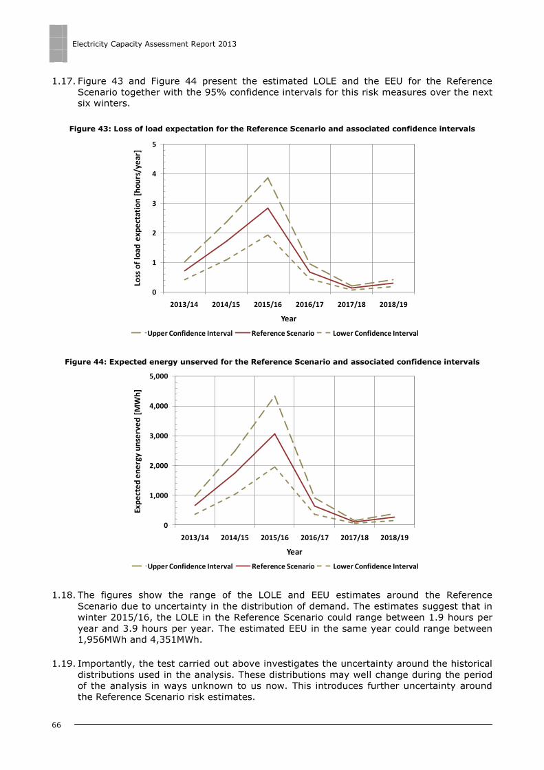
Electricity Capacity Assessment Report 2013
66
1.17. Figure 43 and Figure 44 present the estimated LOLE and the EEU for the Reference
Scenario together with the 95% confidence intervals for this risk measures over the next six winters.
Figure 43: Loss of load expectation for the Reference Scenario and associated confidence intervals
Figure 44: Expected energy unserved for the Reference Scenario and associated confidence intervals
1.18. The figures show the range of the LOLE and EEU estimates around the Reference
Scenario due to uncertainty in the distribution of demand. The estimates suggest that in
winter 2015/16, the LOLE in the Reference Scenario could range between 1.9 hours per
year and 3.9 hours per year. The estimated EEU in the same year could range between 1,956MWh and 4,351MWh.
1.19. Importantly, the test carried out above investigates the uncertainty around the historical
distributions used in the analysis. These distributions may well change during the period
of the analysis in ways unknown to us now. This introduces further uncertainty around
the Reference Scenario risk estimates.
0
1
2
3
4
5
2013/14 2014/15 2015/16 2016/17 2017/18 2018/19
Loss
of
load
exp
ect
atio
n [
ho
urs
/ye
ar]
Year
Upper Confidence Interval Reference Scenario Lower Confidence Interval
0
1,000
2,000
3,000
4,000
5,000
2013/14 2014/15 2015/16 2016/17 2017/18 2018/19
Exp
ect
ed
en
erg
y u
nse
rve
d [
MW
h]
Year
Upper Confidence Interval Reference Scenario Lower Confidence Interval
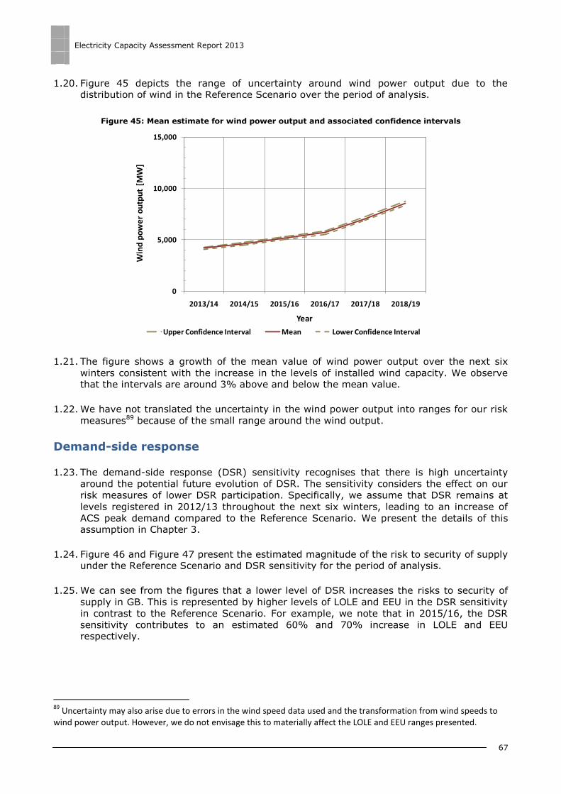
Electricity Capacity Assessment Report 2013
67
1.20. Figure 45 depicts the range of uncertainty around wind power output due to the distribution of wind in the Reference Scenario over the period of analysis.
Figure 45: Mean estimate for wind power output and associated confidence intervals
1.21. The figure shows a growth of the mean value of wind power output over the next six
winters consistent with the increase in the levels of installed wind capacity. We observe that the intervals are around 3% above and below the mean value.
1.22. We have not translated the uncertainty in the wind power output into ranges for our risk
measures89 because of the small range around the wind output.
Demand-side response
1.23. The demand-side response (DSR) sensitivity recognises that there is high uncertainty
around the potential future evolution of DSR. The sensitivity considers the effect on our
risk measures of lower DSR participation. Specifically, we assume that DSR remains at
levels registered in 2012/13 throughout the next six winters, leading to an increase of
ACS peak demand compared to the Reference Scenario. We present the details of this assumption in Chapter 3.
1.24. Figure 46 and Figure 47 present the estimated magnitude of the risk to security of supply under the Reference Scenario and DSR sensitivity for the period of analysis.
1.25. We can see from the figures that a lower level of DSR increases the risks to security of
supply in GB. This is represented by higher levels of LOLE and EEU in the DSR sensitivity
in contrast to the Reference Scenario. For example, we note that in 2015/16, the DSR
sensitivity contributes to an estimated 60% and 70% increase in LOLE and EEU respectively.
89
Uncertainty may also arise due to errors in the wind speed data used and the transformation from wind speeds to wind power output. However, we do not envisage this to materially affect the LOLE and EEU ranges presented.
0
5,000
10,000
15,000
2013/14 2014/15 2015/16 2016/17 2017/18 2018/19
Win
d p
ow
er
ou
tpu
t [M
W]
Year
Upper Confidence Interval Mean Lower Confidence Interval

Electricity Capacity Assessment Report 2013
68
Figure 46: Loss of load expectation for the Reference Scenario and demand-side response
Figure 47: Expected energy unserved for the Reference Scenario and demand-side response
1.26. Figure 48 shows the estimated de-rated capacity margins for the Reference Scenario and DSR sensitivity during the next six winters.
1.27. The figure shows that lower levels of DSR lead to a tighter outlook for de-rated capacity
margins. For instance, in the winter of 2015/16, characterised by the minimum estimated
de-rated margin in the Reference Scenario (ie 3.8%), the DSR sensitivity presents a lower estimated de-rated capacity margin of 2.9%.
0
1
2
3
4
5
2013/14 2014/15 2015/16 2016/17 2017/18 2018/19
Loss
of
load
exp
ect
atio
n [
ho
urs
/ye
ar]
Year
Reference Scenario DSR
0
2,000
4,000
6,000
8,000
10,000
2013/14 2014/15 2015/16 2016/17 2017/18 2018/19
Exp
ect
ed
en
erg
y u
nse
rve
d [
MW
h]
Year
Reference Scenario DSR

Electricity Capacity Assessment Report 2013
69
Figure 48: De-rated capacity margin for the Reference Scenario and demand-side response sensitivity
Gas stress test
1.28. The aim of the gas stress test is to analyse the impact of a drop in gas supplies to GB on
generating capacity margins. Two tests are considered: (i) the potential impact on
margins during an “N-1” event; and (ii) how much gas could be lost from peak day
deliverability before margins are impacted.
1.29. To complete this test we compare demand for gas from the power and non-power sectors
with peak day gas deliverability. If potential demand for gas is higher than peak day
deliverability, then capacity margins may be affected. This is because, such a result would suggest that some gas plant could not be utilised if called upon.
1.30. To undertake both stress tests, we have produced an estimate for total potential gas
demand from the power sector. Based on data from National Grid and Mott MacDonald,
we consider that new CCGT plant is 52% efficient and that plants are running at a
consistent load throughout the day. The results are presented in Table 16 together with
an assumption on the total gas demand from the non-power sector.
Table 16: Potential demand for gas
Gas demand
[MCM/day] 2013/14 2014/15 2015/16 2016/17 2017/18 2018/19
Potential gas demand from power
(Reference Scenario 2013) 120.9 118.0 118.8 122.8 123.9 115.1
Total gas demand from non-power
(National Grid Gas Ten Year Statement 201290)
422.6 417.5 400.2 396.6 389.8 384.5
Total potential gas demand
(potential power plus non-power) 543.5 535.5 519.0 519.4 513.6 499.6
90 National Grid Gas Ten Year Statement 2012. http://www.nationalgrid.com/NR/rdonlyres/E60C7955-5495-4A8A-8E80-8BB4002F602F/58097/GasTenYearStatement2013.pdf
0%
2%
4%
6%
8%
10%
2013/14 2014/15 2015/16 2016/17 2017/18 2018/19
De
-rat
ed
cap
acit
y m
argi
n [
%]
Year
Reference Scenario DSR

Electricity Capacity Assessment Report 2013
70
Test 1: Effect of “N–1” event on capacity margins
1.31. In this test we compare the total potential gas demand against total peak supply
availability during an N-1 event. An n-1 event is equivalent to the loss of the largest
import facility in GB. In this test we assume the loss of Milford Haven91 (86 mcm per
day). The second row in Table 17 shows the impact of an N-1 event on peak supply
availability (shown in row 1). The third row repeats the total potential gas demand figures from Table 16 and the final row presents the surplus supply figures.
Table 17: Gas supply surplus (n-1) and total potential gas demand
Variable
[MCM/day] 2013/14 2014/15 2015/16 2016/17 2017/18 2018/19
Peak supply availability 713.2 723.5 719.1 701.5 685.3 679.6
Peak supply availability
(“n-1” event) 627.2 637.5 633.1 615.5 599.3 593.6
Total potential gas demand 543.5 535.5 519.0 519.4 513.6 499.6
Supply surplus (“n-1” event) 83.7 102.1 114.1 96.1 85.6 94.0
1.32. Table 17 shows that under an N-1 outage event, there is still a large surplus of gas
supplies throughout the period of the analysis. Therefore, an N-1 outage event is not likely to impact our calculated de-rated capacity margins.
Test 2: Potential gas losses before de-rated capacity margins are affected
1.33. We extend the analysis to assess how much peak supply availability could be lost before
the potential demand for gas from power could not be served. Table 18 presents the
surplus supply by subtracting total potential demand for gas from peak supply availability.
Table 18: Gas supply surplus and total potential gas demand
Variable
[MCM/day] 2013/14 2014/15 2015/16 2016/17 2017/18 2018/19
Peak supply availability 713.2 723.5 719.1 701.5 685.3 679.6
Supply surplus 169.7 188.1 200.1 182.1 171.6 180.0
1.34. Table 18 shows that under our assumptions, and depending on the year, between 170
and 200mcm per day of supply availability would have to be lost before de-rated capacity
margins were impacted. This is between 24% and 28% of total gas supply. This range
represents a very significant loss in gas supply availability. Therefore, the likelihood of occurrence is low.
1.35. In addition, it should be highlighted that we have assumed maximum CCGT output for 24
hours and as such the analysis provides an hypothetical maximum demand from CCGT
generation (eg if it were required to run as a baseload source). We would normally expect gas-fired generators to run for only the peak 6 hours of the day92.
91 DECC 2011, “Risk assessment for the purpose of EU Regulation 994/2010 on security of gas supply – An addendum to the Statutory Security of Supply report 2011”, November 2011.
https://www.gov.uk/government/uploads/system/uploads/attachment_data/file/48224/3428-risk-assessment-eu-reg-sec-supply.pdf 92 For further information refer to Ofgem‟s Gas Security of Supply Report:
http://www.ofgem.gov.uk/Markets/WhlMkts/monitoring-energy-security/gas-security-of-supply-report/Documents1/Gas%20SoS%20Report.pdf

Electricity Capacity Assessment Report 2013
71
National Grid Gone Green scenario 2013
1.36. Here we present the levels of risk to security of supply and of the associated de-rated
capacity margins for National Grid‟s Gone Green 2013 scenario over the next six winters.
1.37. In this respect, Figure 46 and Figure 47 illustrate the estimated LOLE and EEU in National
Grid‟s Gone Green 2013 scenario, for the next six winters, together with the Reference Scenario.
Figure 49: Loss of load expectation for the Gone Green 2013 and Reference Scenario
Figure 50: Expected energy unserved for the Gone Green 2013 and Reference Scenario
1.38. Figure 49 shows that the LOLE for next winter 2013/14 is estimated at 0.2 hours per
year in the Gone Green scenario. The LOLE is then expected to increase towards winter
2015/16 when it reaches a level of 1 hour per year. This is largely driven by the closures
of power plant over this period. The LOLE is then estimated to decrease to 0.1 hours per
0
1
2
3
4
5
2013/14 2014/15 2015/16 2016/17 2017/18 2018/19
Loss
of
load
exp
ect
atio
n [
ho
urs
/ye
ar]
Year
Reference Scenario Gone Green
0
1,000
2,000
3,000
4,000
5,000
2013/14 2014/15 2015/16 2016/17 2017/18 2018/19
Exp
ect
ed
en
erg
y u
nse
rve
d [
MW
h]
Year
Reference Scenario Gone Green

Electricity Capacity Assessment Report 2013
72
year in winter 2018/19. This improvement is mainly driven by a decline in electricity demand.
1.39. Figure 47 shows that EEU follows a similar trend to the LOLE over the next six winters in
the Gone Green scenario. For winter 2013/14, the EEU is estimated to be 190MWh. The
estimated EEU then rises in the following two winters to reach approximately 1,031MWh
by 2015/16. As with the LOLE, the estimated EEU falls in the following two winters to reach a low of 69MWh in 2018/19.
1.40. Figure 51 shows the estimated de-rated capacity margins for National Grid‟s Gone Green 2013 scenario and the Reference Scenario over the period of analysis.
Figure 51: De-rated capacity margin for the Gone Green 2013 and the Reference Scenario
1.41. Figure 51 shows that the estimated de-rated capacity margin under National Grid Gone
Green 2013 declines from 8.0% in winter 2013/14, to 5.6% in winter 2015/16 (its lowest
point). This fall is driven by the closure of power plants. Beyond winter 2015/16, the de-
rated margin under Gone Green 2013 rises to a peak of 10.8% in winter 2017/18. This is mainly driven by a decline in electricity demand.
0%
5%
10%
15%
2013/14 2014/15 2015/16 2016/17 2017/18 2018/19
De
-rat
ed
cap
acit
y m
argi
n [
%]
Year
Reference Scenario Gone Green

Electricity Capacity Assessment Report 2013
73
Appendix 2 – Comparing the 2012 and 2013
reports
2.1. In this chapter we compare the headline results of last year‟s Electricity Capacity
Assessment report with those from this report. We first highlight the major differences in
assumptions between the 2012 and 2013 reports. We then present a comparison of the
LOLE and EEU estimates, followed by the de-rated capacity margins. We note that the
Electricity Capacity Assessment report 2012 only estimates risks out to winter 2016/17,
while the results in this report run a further two years to 2018/1993.
2.2. Both reports are structured in a similar way presenting a reference line with sensitivities
to illustrate the impact of variations in the input variables on the results. We refer to the
reference line as Base Case in the 2012 report. In this year‟s report we have decided to
refer to it as Reference Scenario to highlight the fact that it is not intended to be a best
view forecast of future risks but rather a plausible outcome under a particular scenario
defined by a set of assumptions with regards to the main inputs to the analysis (ie
expected supply availability, demand and interconnector flows). The change in the name
does not reflect any changes in the methodology.
Assumptions
2.3. Table 19 illustrates the key differences in Reference Scenario assumptions between the 2012 and 2013 Electricity Capacity Assessment reports.
Table 19: Key Reference Scenario assumption differences between the 2013 and 2012 reports
Year Variable
[MW] 2013/14 2014/15 2015/16 2016/17 2017/18 2018/19
2013
Installed wind capacity 10,208 11,286 12,490 13,802 16,720 20,113
Installed conventional
capacity 67,739 65,941 64,336 65,224 65,634 63,441
ACS peak demand 55,550 55,150 54,590 53,900 53,040 52,340
Largest infeed loss 700 700 700 700 700 700
Net interconnector flows -750 -750 -750 -750 -750 -750
2012
Installed wind capacity 9,485 10,468 11,778 12,981 – –
Installed conventional
capacity 70,025 69,557 67,568 67,761 – –
ACS peak demand 55,734 55,873 55,985 56,173 – –
Largest infeed loss 700 1,572 1,572 1,572 – –
Net interconnector flows -950 -950 -950 -760 – –
Note: (+) Great Britain Imports; (-) Great Britain Exports.
2.4. Table 19 shows that the estimates on the quantity of wind capacity have increased in this
year‟s report. This is in line with updated assumptions from National Grid. On the other
hand our estimates on conventional generation are lower this year. This reflects the
increase in the number of plant that have permanently closed or mothballed since last year and the announcements that some new build will be further delayed.
93 For the capacity assessment report 2013 we have chosen to extend the analysis by one year to capture winter 2018/19 in our analysis, the first year of the Government‟s planned capacity market auctions.
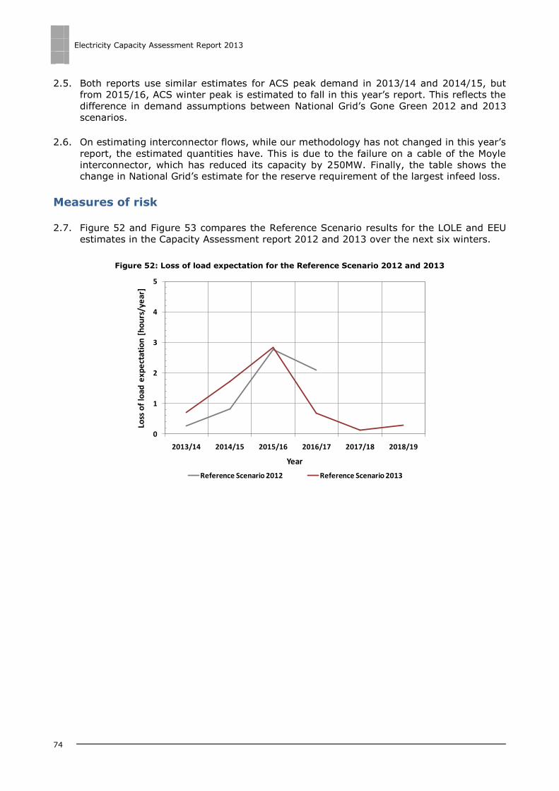
Electricity Capacity Assessment Report 2013
74
2.5. Both reports use similar estimates for ACS peak demand in 2013/14 and 2014/15, but
from 2015/16, ACS winter peak is estimated to fall in this year‟s report. This reflects the
difference in demand assumptions between National Grid‟s Gone Green 2012 and 2013
scenarios.
2.6. On estimating interconnector flows, while our methodology has not changed in this year‟s
report, the estimated quantities have. This is due to the failure on a cable of the Moyle
interconnector, which has reduced its capacity by 250MW. Finally, the table shows the change in National Grid‟s estimate for the reserve requirement of the largest infeed loss.
Measures of risk
2.7. Figure 52 and Figure 53 compares the Reference Scenario results for the LOLE and EEU
estimates in the Capacity Assessment report 2012 and 2013 over the next six winters.
Figure 52: Loss of load expectation for the Reference Scenario 2012 and 2013
0
1
2
3
4
5
2013/14 2014/15 2015/16 2016/17 2017/18 2018/19
Loss
of
load
exp
ect
atio
n [
ho
urs
/ye
ar]
Year
Reference Scenario 2012 Reference Scenario 2013

Electricity Capacity Assessment Report 2013
75
Figure 53: Expected energy unserved for the Reference Scenario 2012 and 2013
2.8. Figure 52 and Figure 53 show that, up to winter 2015/16, the risk of supply shortfalls
measured through LOLE and EEU is higher in this year‟s Capacity Assessment report (red
line) than in last year‟s report (grey line) in the first three years of the analysis. The
increase in the risk levels is largely driven by lower levels of installed capacity compared
with last year‟s report combined with relatively similar levels of electricity demand in the first three winters of the analysis.
2.9. The results in both reports converge to similar levels in 2015/16. This is because the
factors increasing our risk measures in this year‟s report are almost completely balanced
by lower estimated levels of ACS peak demand and increases in estimated installed wind capacity.
2.10. In winter 2016/17, the results diverge significantly, with the estimated LOLE and EEU for
winter 2016/17 considerably lower in the 2013 report. This is driven by the difference in
the electricity demand assumptions in the two reports, with National Grid assuming lower
electricity consumption in this year‟s analysis. In this year‟s report the LOLE in winter
2016/17 is estimated at 0.7 hours per year (compared with 2.1 hours per year in the
2012 report) and the EEU is estimated at 628MWh (compared with 2,494MWh in the 2012 report).
De-rated capacity margin
2.11. Figure 54 compares the Reference Scenario results for the de-rated capacity margins in both Capacity Assessment reports for the next six winters.
0
1,000
2,000
3,000
4,000
5,000
2013/14 2014/15 2015/16 2016/17 2017/18 2018/19
Exp
ect
ed
en
erg
y u
nse
rve
d [
MW
h]
Year
Reference Scenario 2012 Reference Scenario 2013

Electricity Capacity Assessment Report 2013
76
Figure 54: De-rated capacity margin for the Reference Scenario 2012 and 2013
2.12. As expected from the LOLE and EEU results, Figure 54 shows that in the first three years
of our analysis the de-rated capacity margins are lower in the 2013 report than in last
year‟s. In winter 2013/14, the estimated de-rated capacity margin is 6.3%, compared
with the 8.7% de-rated margin expected last year. In winter 2015/16, the two de-rated
capacity margins converge to around 4%. In the following year, the de-rated margins are
now expected to be higher (6.3%) in this year‟s report compared to those estimate last
year (4.8%). This is driven by the lower assumptions on demand that National Grid have provided for this year‟s analysis.
0%
2%
4%
6%
8%
10%
2013/14 2014/15 2015/16 2016/17 2017/18 2018/19
De
-rat
ed
cap
acit
y m
argi
n [
%]
Year
Reference Scenario 2012 Reference Scenario 2013

Electricity Capacity Assessment Report 2013
77
Appendix 3 – Modelling approach
3.1. In this appendix we describe the modelling approach used for the 2013 Electricity
Capacity Assessment report. We first give an overview of the modelling, and then give a description of the model design and structure, including the source of key assumptions.
Overview of the modelling approach
3.2. The primary outputs of the Electricity Capacity Assessment model are:
LOLE: the mean number of hours per year in which supply does not meet demand in the absence of intervention from the System Operator.
EEU: the mean amount of electricity demand that is not met in a year. EEU combines both the likelihood and the potential size of any supply shortfall.
Frequency and duration of expected outages: an illustration of the results of the
probabilistic risk measures in terms of tangible impacts for electricity customers. This is
based on judgements around how the electricity system would operate at a time when
supply does not meet demand, and the order and size of mitigation actions taken by
the System Operator. It is therefore not as accurate as the LOLE and EEU but it allows
us to provide a view of the probability of experiencing controlled disconnections of customers.
EFC: the quantity of firm capacity (ie always available) that can be replaced by a
certain volume of wind generation to give the same level of security of supply, as
measured by LOLE. This measure is used to calculate the average contribution of wind
power to the de-rated margin. It varies with the proportion of wind power in the system.
De-rated capacity margin: the average excess of available generation capacity over
peak demand, expressed in percentage terms. Available generation capacity takes into
account the contribution of installed capacity at peak demand by adjusting it by the
appropriate de-rating (or availability) factors which take into account the fact that plant are sometimes unavailable due to outages.
3.3. LOLE is not a measure of the expected number of hours per year in which customers may
be disconnected. We define LOLE to indicate the number of hours in which the system
may need to respond to tight conditions.
3.4. For a given level of LOLE and EEU, results may come from a large number of small
events where demand exceeds supply in principle but it can be managed by National Grid
through a set of mitigation actions available to them as System Operator94. The results
may also come from a small number of large events (eg the supply deficit is more than 2
to 3GWh95) where controlled disconnections cannot be avoided. Conversely, given the
characteristics of the GB system, any shortfall is more likely to take the form of a large number of small events that would not have a direct impact on customers.
94 The System Operator can implement mitigation actions to maintain the system when available supply is insufficient to meet demand. These include voltage control, maximum generation instruction and emergency services from the interconnectors. 95 This varies with the specific conditions of the market at the time of the outage, including the flows over the interconnectors at the time.

Electricity Capacity Assessment Report 2013
78
3.5. LOLE serves to take account of the impact of rising levels of variable generation.
However, it may not reflect any potential improvements96 in the capacity of the system
to cope with more variability before any disconnections. We do not expect these
improvements to have a significant impact in the market in the next six winters.
Sensitivity development
3.6. A key part of this study has been to develop a Reference Scenario for the future
electricity demand and supply background over the next six winters. This Reference Scenario covers assumptions on:
Electricity demand at ACS peak;
Installed generation capacity, including new builds, retirements and mothballing;
Interconnector capacity and imports/exports at peak;
Generator availabilities.
3.7. A set of sensitivities has also been developed to test the impact on capacity adequacy of key uncertainties in the Reference Scenario assumptions.
Probabilistic model
3.8. Under normal circumstances there is a margin of generation capacity over electricity
demand. The risks of supply shortfalls due to inadequate capacity occur at the extremes
of high demand and/or low availability of generation capacity. We therefore take a
probabilistic approach, using recent history to estimate the possible ranges of electricity
demand and supply, and hence the distribution, at any time, of the excess of supply over
demand. This distribution forms the basis of the estimation of the primary outputs of
each assessment, ie LOLE and EEU. We further test the sensitivity of these outputs to
variation in input assumptions. The latter include, among other, varying views of future
capacity and electricity demand, together with assumptions about their statistical relationship as they vary over time.
3.9. The constructed model is a probabilistic model of capacity adequacy in the GB electricity
market, and corresponds in turn to each of the next six winters. It is a time-collapsed
model; it models the joint distribution of available conventional generation capacity X,
wind generation capacity W and electricity demand D at a typical, or randomly chosen,
half-hourly period of the winter under study. This time-collapsed model is sufficient to
calculate the distribution of the surplus Z = X + W - D at such a randomly chosen time, together with the primary outputs LOLE and EEU.
3.10. The model takes no account of the chronological ordering of the half-hourly time periods
of the winter under study. However, both the expected frequency and duration of
outages depend on this ordering. Thus, in order to provide estimates of the latter
quantities, it is necessary to combine the model with further information.
96 One potential improvement would be for example further penetration of frequency management through automated appliances. For further information refer to:
http://www.ofgem.gov.uk/Pages/MoreInformation.aspx?file=20130430_Creating%20the%20right%20environment%20for%20demand-side%20response.pdf&refer=Markets/sm/strategy/dsr

Electricity Capacity Assessment Report 2013
79
3.11. The distribution of demand is based on recent historical half hourly demand for electricity
on the system, for the winters 2005/06 to 2012/13. This distribution is adjusted for the
scenario assumption on peak demand in each winter.
3.12. The distribution of future generation capacity availability is built up from two distributions
with distinctly different characteristics. The conventional (non-wind) capacity distribution
is calculated using the installed capacity and the mean winter availability of each
generating unit. The mean availability has been estimated from historical data, covering
the period from 2005/06 to 2011/12. The distribution of wind output availability is
calculated from historical wind speed data covering the period from 1979 to 2012 for current and future GB wind farm locations.
3.13. The random variables X, W and D are assumed to be independent. In order to take
account of possible statistical association between wind generation W and demand D, the
distribution of W is estimated from wind data corresponding to the winter season. The distribution of Z is then obtained by the convolution97 of the distributions of X, W and -D.
3.14. Figure 55 shows a schematic representation of the combination of distributions of supply
and demand. The mean of the generation capacity availability distribution is higher than
the mean of the demand distribution. There is a high, but not 100%, probability that supply exceeds demand.
Figure 55: Schematic diagram of electricity demand and capacity distributions
3.15. The model calculates two well-established metrics of security of supply, the Loss of Load
Expectation (LOLE) and the Expected Energy Unserved (EEU). The LOLE is the mean
number of periods per year in which supply does not meet demand, in the absence of
intervention from the System Operator. The EEU is the corresponding volume of demand
that is expected not to be met during the year. The LOLE and EEU are derived from the
Loss of Load Probability (LOLP) and Expected Power Unserved (EPU). The LOLP is the
probability of demand exceeding supply, and the EPU is the corresponding volume of
demand that is expected not to be met, during a randomly chosen half-hourly period. LOLP and EPU are formally defined as follows:
97 Convolution is the mathematical operation of obtaining the distribution of the sum of two independent random variables from their individual distributions. See for example, R. Durrett, Probability: Theory and Examples, 4th ed. Cambridge University Press, 2010.
0.00%
0.20%
0.40%
0.60%
0.80%
1.00%
1.20%
1.40%
20
00
0
22
70
0
25
40
0
28
10
0
30
80
0
33
50
0
36
20
0
38
90
0
41
60
0
44
30
0
47
00
0
49
70
0
52
40
0
55
10
0
57
80
0
60
50
0
63
20
0
65
90
0
68
60
0
Pro
bab
ility
(%
)
MW
Generation availability
Demand
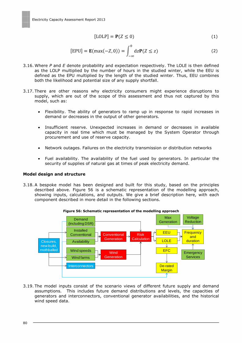
Electricity Capacity Assessment Report 2013
80
(1)
(2)
3.16. Where P and E denote probability and expectation respectively. The LOLE is then defined
as the LOLP multiplied by the number of hours in the studied winter, while the EEU is
defined as the EPU multiplied by the length of the studied winter. Thus, EEU combines both the likelihood and potential size of any supply shortfall.
3.17. There are other reasons why electricity consumers might experience disruptions to
supply, which are out of the scope of this assessment and thus not captured by this model, such as:
Flexibility. The ability of generators to ramp up in response to rapid increases in demand or decreases in the output of other generators.
Insufficient reserve. Unexpected increases in demand or decreases in available
capacity in real time which must be managed by the System Operator through
procurement and use of reserve capacity.
Network outages. Failures on the electricity transmission or distribution networks
Fuel availability. The availability of the fuel used by generators. In particular the
security of supplies of natural gas at times of peak electricity demand.
Model design and structure
3.18. A bespoke model has been designed and built for this study, based on the principles
described above. Figure 56 is a schematic representation of the modelling approach,
showing inputs, calculations, and outputs. We give a brief description here, with each component described in more detail in the following sections.
Figure 56: Schematic representation of the modelling approach
3.19. The model inputs consist of the scenario views of different future supply and demand
assumptions. This includes future demand distributions and levels, the capacities of
generators and interconnectors, conventional generator availabilities, and the historical wind speed data.
Demand
(including DSR)
Wind
Generation
Conventional
Generation
Wind speeds
Wind farms
Installed
Conventional
Availability
Risk
Calculation
EEU
LOLE
Frequency
and duration
Voltage
Reduction
Interconnectors
EFC
De-rated
Margin
Emergency
Services
Closures,
new build, mothballed
Max
Generation

Electricity Capacity Assessment Report 2013
81
3.20. There are two major calculation modules. The first deals with the construction of the
wind distribution, and the second does the calculations of the security of supply metrics.
These are covered in more detail in the relevant sections below.
3.21. The outputs are the LOLE and EEU results and the additional metrics of the frequency and duration of outages.
3.22. In addition, we calculate a commonly used indicator of security of supply: the de-rated
capacity margin. The de-rated margin represents the average excess of available
generation capacity over peak demand and is expressed in percentage terms. Available
generation takes into account the contribution of installed capacity at peak demand by adjusting it by the appropriate de-rating factors.
Assumptions
3.23. Table 1 provides a summary of the sources used to derive the assumptions for the main inputs of the model.
Table 20: Summary of common assumptions and data sources
Assumption Source
Demand distribution
Historical Indicative Demand Outturn (INDO) data for
2005/06 to 2012/13 for the period in which GB is on Greenwich Mean Time. INDO data has been available
since the formation of the GB BETTA98 market in 2005. Defines the demand profile
ACS Peak demand
Sensitivity variable. For Reference Scenario, source is
National Grid‟s Gone Green 2013 scenario for the Future Energy Scenarios. Defines the overall level of demand
growth.
Installed capacity
Sensitivity variable. For Reference Scenario, the primary
source is National Grid‟s Gone Green 2013 scenario for the Future Energy Scenarios with amendments to reflect Ofgem‟s views. This provides the full portfolio of installed
capacity for the next six winters.
Embedded wind capacity National Grid‟s assumptions for Gone Green 2013.
Conventional plant availability Analysis of historical Maximum Export Limit (MEL) data
and planned outage data.
Wind speed data MERRA re-analysis data set.
Wind turbine power curves Manufacturer data adjusted for actual operation of wind
turbines.
Wind farm locations National Grid internal research.
Interconnector capacities Based on Ofgem‟s assumptions.
Interconnector peak flow Sensitivity variable. For Reference Scenario, the primary
source is Ofgem‟s and Pöyry‟s analysis.
Demand-side Response Sensitivity variable. For the Reference Scenario, the
primary source is National Grid Gone Green 2013 scenario
Demand
3.24. The starting point for the distribution of demand is the historical half hourly demand of
the winters since winter 2005/06. This data is the Indicative Demand Outturn (INDO)
data, available for GB as a whole since the introduction of the British Electricity Trading Arrangements (BETTA) in 2005.
98 British Electricity Trading Transmission Arrangements.
Electricity Capacity Assessment Report 2013
82
3.25. The distribution of each historical winter is rebased against the ACS peak demand value for that historical year.
3.26. For each historical year, the generation from embedded wind has been estimated using
the wind model and added onto demand. The purpose of this is to allow all wind (both
embedded and transmission connected) to be modelled explicitly on a consistent basis in
the model.
3.27. To account for overall growth in demand, the distribution is scaled by the forward looking assumptions for ACS peak.
3.28. For each of the next six winters, the highest demand in the distribution is higher than the
quoted ACS peak demand, by about 1.8GW. The difference exists for two reasons.
Firstly, ACS peak does not represent the outturn peak in any one year. ACS peak
demand is a value that is calculated to remove the effects of weather fluctuations on
peak demand. To calculate the ACS peak demand, the actual peak value is adjusted to
the demand that would have been expected in an average cold spell. If the peak day is
colder than the average cold spell, then the outturn peak will be higher than the reported ACS value.
3.29. Secondly, the demand distribution used in the model includes demand met by embedded wind, and so is higher than the ACS peak which does not include embedded wind.
3.30. The demand distribution for each of the future winters is a direct input to the risk assessment calculation.
Conventional generation
3.31. For the purposes of this study, when we refer to conventional generation capacity we mean the non-wind generators connected to the GB transmission system.
3.32. A standard approach to modelling the availability of conventional generators is to treat
each generator as being either fully available or completely unavailable. Each generator is assigned a probability of being available, estimated from historical data.
3.33. The exception is for CCGTs which contain multiple Gas Turbine (GT) units. In this case, the failure of each GT unit has been modelled individually.
3.34. The availability assumptions for each generator type are estimated from analysis of
historical availability as submitted by generators to National Grid. The data used is the
Maximum Export Limit (MEL) submitted by generators for the winters from 2005/06 to
2011/12. The MEL data submitted by generators is commercial and a generator may
declare itself unavailable for a number of reasons. There may be a planned maintenance
outage, or a forced (unplanned) outage, or commercial reasons not directly related to technical availability.
3.35. We estimate the availability of each generator type at times of high winter demand for
every winter. In particular, we are considering days with a demand level higher than the
50th percentile of winter peak demand. By considering periods of high winter demand the
calculated availability represents a realistic estimate of what the generator is capable of generating at times of high demand, including rescheduling of any planned maintenance.

Electricity Capacity Assessment Report 2013
83
3.36. The Reference Scenario availability is defined as the mean availability of the seven winter
estimates. The availability values used for the low (high) availability sensitivities are
defined as the mean minus (plus) one standard deviation of the seven winter estimates.
3.37. The final mean availability assumptions used in the Reference Scenario and sensitivities are shown in Table 21.
Table 21: Generator availability per technology type
Fuel type Availability [%]
Low Reference Scenario High
Coal / Biomass 86% 88% 90%
Gas CCGT / Gas CHP 81% 85% 89%
OCGT 87% 92% 97%
Oil 75% 82% 89%
Nuclear 76% 81% 86%
Hydro 78% 84% 90%
Pumped Storage 93% 96% 99%
3.38. The availability and capacities of individual generators are combined into a single
capacity outage table, which is a distribution of the aggregate available capacity.
Wind generation
3.39. The source for wind speed data is NASA‟s Modern Era Retrospective-analysis for Research
and Applications (MERRA) reanalysis dataset99. This is a long term (1979-2012) dataset
built up from analysis of remote sensor (satellite) data. The full dataset is global in coverage and contains information on all aspects of climate.
3.40. For the purposes of this study, a subset of the MERRA data has been downloaded. The
subset contains wind speeds at 2m, 10m and 50m height, for a grid covering the British
Isles. The grid is at 0.5 degree longitude by 0.75 degree latitude which corresponds to
approximately 50km spacing over GB. The model uses this data in combination with the
capacity, hub height and coordinates of all transmission connected and embedded wind in GB.
3.41. To access the raw data, University of Reading were contracted to build an extraction tool.
The tool is written in FORTRAN90 and compiled into a form which can be run on a
standard Windows PC. The detailed description of this tool is online100. The tool can be
run stand alone to extract the wind speed data for an individual wind farm location over a
specified period of time (1979-2012). The tool interpolates between local grid points to
derive the wind speed for the specified location. It also adjusts for hub height using a logarithmic relationship.
Conversion from wind speed to wind power output
3.42. The wind output is estimated for each wind farm under consideration in GB. For a specific
wind farm the latitude, longitude and hub height are input into the wind tool to generate
a wind speed time series. The wind speed time series is converted into a wind load factor
time series using a wind power (load factor) curve. Finally the wind load factor time
99 MERRA data used in this project have been provided by the Global Modelling and Assimilation Office (GMAO) at NASA Goddard Space Flight Center through the NASA GES DISC online archive. https://gmao.gsfc.nasa.gov/merra/ 100 University of Reading Wind profile program documentation: http://www.met.reading.ac.uk/~marc/it/wind/

Electricity Capacity Assessment Report 2013
84
series is multiplied by the installed capacity of the respective wind farm to produce the wind output from this wind farm.
3.43. The process for constructing the wind power curve is detailed below. This is a different
approach from the 2012 analysis in which we used typical wind power curves from manufacturers to convert wind speeds to wind power output.
3.44. The wind power curve was constructed by using actual output data from 9, randomly
chosen, wind farms that are currently generating, and is applied on both onshore and
offshore wind101. Specifically, the actual output time series of the 9 wind farms was
converted into a load factor time series by dividing with the installed capacity of the
respective wind farm. An S-curve102 was subsequently fitted to the load factor data using
a non-linear squares method103. A cut-out speed of 25 m/sec was chosen with a standard
deviation of 1.5 m/sec, as this is typically given by wind farm manufacturers as a cut-out speed.
3.45. Figure 57 presents the wind power curve used in the 2013 and 2012 analysis. The 2013
approach has two advantages over the 2012 approach:
The 2013 methodology intrinsically accounts for any wind turbine unavailability, based on historical data;
It models the behaviour of a group of turbines rather than the behaviour of an
individual turbine. This accounts for the geographic dispersion of wind turbines in a wind farm, as the wind speed varies from turbine to turbine in a wind farm.
Figure 57: Wind power curve in the 2013 and 2012 analysis104
101 We use the same wind power curve for both onshore and offshore turbines as the main difference in output is due to wind speeds being higher offshore. 102 The S-curve is given by the following formula: , where w/s is the MERRA wind speed
and A, B and C are the parameters which characterise the fit. 103 As there is very few data at high wind speeds to fit a cut-out S-curve using a non-linear least squares method, one was fitted by inspection. 104 The grey shaded area indicates the actual MW metered data used to calibrate the 2013 model. Darker areas indicate a higher density of data points.
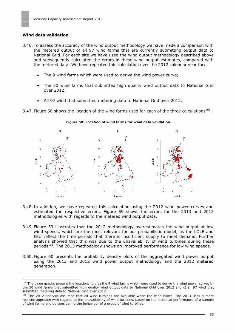
Electricity Capacity Assessment Report 2013
85
Wind data validation
3.46. To assess the accuracy of the wind output methodology we have made a comparison with
the metered output of all 97 wind farms that are currently submitting output data to
National Grid. For each site we have used the wind output methodology described above
and subsequently calculated the errors in these wind output estimates, compared with the metered data. We have repeated this calculation over the 2012 calendar year for:
The 9 wind farms which were used to derive the wind power curve;
The 50 wind farms that submitted high quality wind output data to National Grid over 2012;
All 97 wind that submitted metering data to National Grid over 2012.
3.47. Figure 58 shows the location of the wind farms used for each of the three calculations105.
Figure 58: Location of wind farms for wind data validation
3.48. In addition, we have repeated this calculation using the 2012 wind power curves and
estimated the respective errors. Figure 59 shows the errors for the 2013 and 2012 methodologies with regards to the metered wind output data.
3.49. Figure 59 illustrates that the 2012 methodology overestimates the wind output at low
wind speeds, which are the most relevant for our probabilistic model, as the LOLE and
EEU reflect the time periods that there is insufficient supply to meet demand. Further
analysis showed that this was due to the unavailability of wind turbines during these periods106. The 2013 methodology shows an improved performance for low wind speeds.
3.50. Figure 60 presents the probability density plots of the aggregated wind power output
using the 2013 and 2012 wind power output methodology and the 2012 metered generation.
105 The three graphs present the locations for: a) the 9 wind farms which were used to derive the wind power curve; b) the 50 wind farms that submitted high quality wind output data to National Grid over 2012 and c) all 97 wind that submitted metering data to National Grid over 2012. 106 The 2012 analysis assumed that all wind turbines are available when the wind blows. The 2013 uses a more realistic approach with regards to the unavailability of wind turbines, based on the historical performance of a sample of wind farms and by considering the behaviour of a group of wind turbines.

Electricity Capacity Assessment Report 2013
86
Figure 59: Distribution of errors for 2013 and 2012 wind power output methodologies – with regards to 2012 metered data
Figure 60: Probability density plots of the aggregate wind power output of the wind farms over 2012
Wind output distributions
3.51. For the capacity assessment model, wind output distributions are generated for each of
the six winters for which the capacity assessment is performed. The distributions are
calculated from the scenario capacity mix, combined with the full set of wind speed data (1979-2012).
3.52. A single aggregate distribution of wind generation is created for each year. The installed
wind capacity in 2013/2014 is 10.2GW, and by 2018/2019 this has increased to 20.1GW. There is nearly a zero probability of there being no output at all from wind.
3.53. The wind distribution for each capacity year is convolved with the distributions of
conventional generation and demand to create a distribution of the margin of supply over demand. The key metrics of LOLE and EEU are calculated from this distribution.

Electricity Capacity Assessment Report 2013
87
Equivalent Firm Capacity
3.54. The wind distributions above show that a large range of wind output levels can occur,
with varying probabilities. It is useful to be able to translate this into an equivalent
amount of firm capacity which provides the same contribution to security of supply, where the contribution to security of supply is measured in terms of LOLE or EEU.
3.55. We therefore use a standard measure known as Equivalent Firm Capacity (EFC). This is
the amount of capacity that is required to replace the wind capacity to achieve the same level of LOLE. It is specific to a particular capacity and demand background.
3.56. EFC is a measure of the capacity adequacy provided by wind and it varies with the
proportion of wind in the generation mix. A key use of the EFC is in the calculation of de-
rated capacity margins, where the aim is to reflect the contribution of each generation
type to capacity adequacy. It does not provide any insight on operational issues such as
errors in wind forecasting.
3.57. For illustration, Figure 61 shows, for a given wind distribution, the average winter load
factor and the EFC. At very small installed capacity of wind, the EFC is close to the mean
availability of wind. As the installed capacity of wind and the proportion of wind in the
system increases, the value of EFC drops as the possibility of near zero wind output, GB-
wide, becomes increasingly important in determining wind‟s contribution within the risk calculation.
Figure 61: Comparison of wind distribution, average winter load factor and EFC
3.58. The EFCs calculated in this study are higher than other values that have been quoted for
the contribution of wind to security of supply. For example, National Grid have previously
used a value of 8% in the Winter Outlook 2011/12. Also, the value of EFC varies year on
year in our analysis while similar report may assume a constant figure over the period of
analysis.
3.59. The large difference in these numbers reflects two very different approaches. The Winter
Outlook approach is based on observations of the output of wind at peak times. By its
nature this is a small number of observations, and it is therefore possible that the wind output at the time of observation could have been very different.
0
2000
4000
6000
8000
10000
12000
14000
0% 10% 20% 30% 40% 50% 60% 70% 80% 90% 100%
Ge
ne
rati
on
(MW
)
Probability of output greater than level
2016/17 EFC MeanWind
power

Electricity Capacity Assessment Report 2013
88
3.60. We do not consider this approach appropriate for a capacity adequacy analysis, as it
represents a pessimistic estimate of the availability of wind in isolation from the rest of the system.
3.61. In contrast, EFC is a statistical approach which takes account of the change in risk to
security of supply due to the intermittent nature of wind output. The EFC value depends
on both the system background scenario (ie generation and demand scenario) and the
variability of wind. It recognises that the system already has some non-zero risk, and
aims to calculate the level to which wind can be relied on so as to not increase this
risk107.
Treatment of special cases
3.62. Here we discuss the treatment of special cases covering interconnectors, Demand-side
Response (DSR), pumped storage and embedded generation.
3.63. Imports or exports on interconnectors to Ireland or mainland Europe are modelled as a
decrease or increase in demand respectively. The assumptions on imports or exports
over the interconnectors at peak vary between sensitivities. Exports are added directly
to the demand distribution, and imports are subtracted from the distribution.
3.64. The availability of generation from pumped storage is modelled as conventional
generation. The model does not take account of any constraints that may be imposed by
the capacity of the storage, which could potentially limit the availability of generation
from pumped storage across the peak period. Supporting analysis by National Grid
suggests that the pumped storage generators have sufficient storage to operate across
the peak period. This suggests that this limitation of the modelling is not significant for the five winters modelled.
3.65. Demand-side Response is assumed to grow in the Reference Scenario over the course of
the analysis period. The model makes use of the actual historical demand data which
already includes any demand reduction due to DSR. Using the historical data directly
means that the impact of the current level of DSR is included in the model. We assume
that DSR participation grows over the six winter modelling period, both in the domestic and non-domestic sector. This follows National Grid‟s Gone Green 2013 work.
3.66. The historical demand data used is for demand met on the transmission system.
Generation from embedded generators manifests as a decrease in demand on the
transmission system. In this study, embedded wind generation is modelled explicitly as
generation, and therefore the historical demand distribution is increased by an estimate
of the demand met by embedded wind historically in each half hour. All other embedded
generation (consisting of a range of technologies including for example small scale
Combined Heat & Power, generation from landfill gas, and biomass) is implicitly modelled
in the demand data. Growth in embedded generation is reflected in the projected ACS
peak demand.
Calculation of outputs
3.67. The distributions of conventional capacity and wind are combined to form a single
distribution of generation capacity. The demand distribution is then subtracted to form a distribution of margins of supply over demand.
107 For further information refer to: S. Zachary and C. J. Dent, “Probability theory of capacity value of additional generation,” J. Risk and Reliability, vol. 226, no. 1, pp. 33-43, 2012.

Electricity Capacity Assessment Report 2013
89
3.68. There is a small portion of the distribution for which demand exceeds supply and margins
are negative. This is the left hand side of the distribution illustrated in Figure 62. Each
bar represents the expectation of the number of half hours per year that the margin will be in that 100 MW tranche.
Figure 62: Illustration of a distribution of de-rated margins
3.69. The distribution of margins is used to calculate the risk and the impact of supply
shortfalls by including two well-established probabilistic measures of security of supply
analysis: LOLE and EEU. In addition, we calculate a commonly used indicator of security
of supply: the de-rated capacity margin.
3.70. The calculation of the de-rated margin is shown schematically in Figure 63 below. There
are three components: demand, wind generation and conventional generation
availability. The de-rated margin can be stated in percentage terms as the average
excess of generator availability, divided by peak demand. The de-rated margin is defined
as follows:
(3)
3.71. Where net exports are added to (subtracted from) the ACS peak demand if GB is a net exporter (importer) and LIF represents the largest infeed loss reserve requirement.
0.0000
0.0005
0.0010
0.0015
0.0020
0.0025
0.0030
0.0035
0.0040
-30
00
-27
00
-24
00
-21
00
-18
00
-15
00
-120
0
-90
0
-60
0
-30
0 0
300
600
900
120
0
1500
1800
Hal
f h
ou
rs p
er y
ear

Electricity Capacity Assessment Report 2013
90
Figure 63: Calculation of de-rated capacity margin
3.72. For demand, we use the ACS peak demand. As described above, it is possible for outturn
demand to exceed this level. We also adjust at this point for the amount of generation
that must be held as reserve to protect the integrity of the system against the largest
infeed loss. Net exports (imports) over the interconnectors (which vary by sensitivity) are added to (subtracted from) demand.
3.73. For conventional generation, the installed capacity of each generation type is multiplied
by the mean availability of that type. The assumed availabilities are shown in Table 21.
3.74. For wind capacity, the average availability of wind is not suitable as this would overstate
the contribution of wind to security of supply. A more suitable value is the Equivalent
Firm Capacity (EFC), estimated from the probabilistic model as described above. The
model calculates the amount of firm capacity that would be needed to replace the wind
capacity to give the same LOLE. This is lower than the mean winter load factor because of the chance that wind output could be very low.
3.75. The EFC is specific to any one sensitivity and year because it is dependent on the
proportion of wind power in the overall generation mix. The Reference Scenario produces
EFC values that are typically in the range of around 17 – 23%. At very small capacity of
installed wind, the EFC is close to the mean winter load factor for wind. As the installed
capacity of wind increases, the EFC value decreases, as the possibility of near-zero wind
production, system-wide, becomes increasingly important in determining the contribution
of wind to the risk calculation.
3.76. The de-rated capacity margin also includes an adjustment for assumed flows on the
interconnectors and the reserve held by the System Operator for single largest infeed
loss. This type of reserve is required in order to maintain the stability and integrity of the
system, and therefore disconnection of demand would occur ahead of using this reserve
(whereas other forms of reserve would be used to prevent supply shortfalls108). As it is a
form of reserve that must be maintained, we therefore include it as “demand” in the analysis.
3.77. The interconnection and reserve adjustment are applied as increases to GB demand. The assumptions for the Reference Scenario are shown in Table 22 below.
108 This reserve is a sub-set of the full reserve requirement that the SO holds in order to manage the system on operational timescales.
ACS peak
demand
Mean of Net
generation
distribution
Risk calculation Equivalent Firm
Capacity (EFC)
of wind
De-rated
margin
Demand
Wind
Conventional

Electricity Capacity Assessment Report 2013
91
Table 22: Interconnector flow assumptions (in GW) at winter peak periods for sensitivities
Variable
[MW] 2013/14 2014/15 2015/16 2016/17 2017/18 2018/19
ACS Peak Demand 55,550 55,150 54,590 53,900 53,040 52,340
Exports to Ireland 750 750 750 750 750 750
Reserve for Largest Infeed Loss 700 700 700 700 700 700
Adjusted ACS peak demand 57,000 56,600 56,040 55,350 54,490 53,790
Frequency and duration of outages
3.78. For illustration, we have translated the risk metrics, LOLE and EEU, into the possible
effects on electricity customers. We estimate the likely frequency and duration of
shortfalls in supply and categorise these outages by severity. The categories are defined
by the potential mitigating measures which may be available to the System Operator. These measures can be seen in Table 23.
Table 23: Mitigation measures
Action Comments Assumed effect
[MW]
Voltage reduction Reduce demand by instructing distribution network owners
(DNOs) to reduce voltage 500
Maximum generation Increase in supply by instructing generating plants to increase
generation to maximum 250
Provision of emergency
services through interconnection
Increase in supply through interconnection services with
neighbouring markets (various services available, eg Emergency Instruction, Emergency Assistance and Cross-Border Balancing)
2,000
3.79. The probabilistic model does not produce the frequency and duration of outages directly
as it does not account for the chronological ordering of the time periods. We can
estimate the frequency and duration of outages using the following additional assumptions:
We assume that outages occur on a typical peak demand day (a weekday in January).
We assume that the conventional plant availability is constant over the duration of
an outage. This is reasonable given that typical repair times are longer than the peak period.
We assume that the wind availability does not change over the duration of an
outage. This is an approximation that is reasonable given the level of wind
generation in the time horizon of the modelling, but which will become less valid in
future winters.
3.80. Using the minute by minute demand profile for the typical peak demand day, the total
duration of an outage may be defined as the length of continuous time for which demand
exceeds supply. The maximum severity of this outage (GW) is the maximum value of
the excess of demand over supply, and it is possible to estimate the mean length of time,
during the outage, at which the shortfall is at this maximum value. For each level of
shortfall which is lower than the maximum, it is similarly possible to estimate the mean
length of time, during the outage, at which the shortfall is at this lower level. Controlled
disconnections occur after voltage reduction, maximum generation services and emergency services from interconnectors have been exhausted.

Electricity Capacity Assessment Report 2013
92
3.81. Given this set of outage types, typically characterised by their maximum levels of
severity, for each year and sensitivity we need to find the frequency of each outage type.
These frequencies need to be consistent with the outputs of the earlier probabilistic
model. To describe the analysis, for each outage type k, let fk denote the annual
frequency of outages of this type, and, for each loss of load of j GW, let μkj denote the mean length of time (hours) that such an outage lasts. Then, for each j
(4)
3.82. Where Nj is the expected number of hours per year at which the loss of load is j. The Nj
are the fundamental outputs of the earlier probabilistic model; indeed we have:
(5)
(6)
3.83. Where J is the maximum loss of load with a non-negligible probability. Given the earlier
estimates of the μk,j, the equations (4) (which are J equations in K unknowns) may now
be solved for the required frequencies fk. For example, if outage type k corresponds to a
maximum loss of load during the outage of k GW, so that K = J and, for each k we have
μk,j = 0 for j > k, then the equations (4) may be solved recursively, starting with j = J, to determine uniquely all the fk
109.
3.84. The final values are thus a set of frequencies (1-in-n years) for each shortfall category.
The results should be considered approximate only, due to the additional assumptions
required. There is also a risk that each of the mitigation measures may not be fully
available to the System Operator when required.
Uncertainty analysis
3.85. In this section we describe the approach to quantifying the uncertainty inherent in this
analysis.
3.86. The uncertainty can be characterised into three types:
Statistical (internal) uncertainty
109 As a simple numerical example, which is intended for illustration only, suppose that the daily demand curves suggest that there are just two shortfall types: type 1 shortfalls correspond to an outage of 1GW and have a mean duration of μ1,1 = 1hr, while type 2 shortfalls correspond to an outage of 2GW with a mean duration of μ2,2 = 2hrs, coupled with an outage of 1GW with a further mean duration of μ2,1 = 3 hrs. The equations (5 and 6) then become
N1 = f1 + 3f2
N2 = 2f2
giving f2 = N2/2 and then f1 = N1 – 3N2/2.
If the expected number of hours in the year at which the loss of load is 1GW is given by N1 = 0.13, while the expected number of hours in the year at which the loss of load is 2GW is given by N2 = 0.02, then we have f1 = 0.1 and f2 = 0.01. Thus type 1 shortfalls occur on average 1 year in 10, while type 2 shortfalls occur on average 1 year in 100.

Electricity Capacity Assessment Report 2013
93
Uncertainty due to independence assumptions within the model
Uncertainty due to non-statistical modelling assumptions
3.87. Statistical (internal) uncertainty is the uncertainty in the probability distributions derived
from historical data, in this case the probability distributions of demand and wind. It
arises from the natural randomness in the finite sample of data used in the analysis.
3.88. Uncertainty in the probability distributions derived from historical data can be estimated
through a resampling technique known as bootstrapping. This technique uses sampling
with replacement from within the dataset to produce bootstrap samples. Each of these
bootstrap samples is then used to re-estimate the output quantity of interest, eg LOLE or
EEU. The resampling of the data is done in blocks sufficiently large as to be considered
independent of each other. The variability in the re-estimated quantities then provides a reasonable measure of the uncertainty due to the finiteness of the input data.
3.89. In the case of demand, bootstrapping has been used to estimate 95% confidence
intervals for LOLE and EEU based on the uncertainty in the demand distribution. The
demand is divided into weekly blocks which are assumed to be independent, then
resampled many times to produce a large number of bootstrap samples. Each sample
produces a different estimate for LOLE and EEU. We thus find 95% confidence intervals
for LOLE and EEU.
3.90. A similar technique may in principle be used to assess the uncertainty due to the
finiteness of the wind data. However the feasibility of this approach depends on
managing the large computational overhead in the processing of this data. Due to the
computational overhead of processing the wind data, it has not been possible to estimate
the confidence intervals on LOLE and EEU. However, it has been possible to examine the
confidence intervals in the wind distribution itself, which gives some insight into the scale
of this uncertainty. In addition, uncertainty in the distribution of wind generation may
well be dominated by the uncertainty in the assumption that wind generation is
independent of demand. The latter uncertainty is discussed below.
3.91. The distribution of conventional plant availability is derived from historical analysis of
outage rates, and the uncertainty in this distribution is best characterised through sensitivity analysis of the outage rates.
3.92. The assumption of independence of distributions is a source of uncertainty. The
assumption that wind and demand are independent at times of system peak is a
reasonable assumption given that there is no well characterised statistical relationship
between the two. This assumption is an uncertainty which is tested to some extent through the low wind generation sensitivity.
3.93. Table 24 summarises the approach to the uncertainties on various parameters in the
modelling.

Electricity Capacity Assessment Report 2013
94
Table 24: Summary of approach to treatment of uncertainties
Uncertainty source Uncertainty type Approach
Demand Statistical (internal) Bootstrapping &sensitivity analysis
Wind Statistical (internal) and data source,
but dominated by independence assumption
Bootstrapping & sensitivity analysis
Distribution of conventional capacity Dominated by modelling assumptions about plant availability probabilities
Sensitivity analysis
Assumption of independence of
demand and wind at time of extreme demand
Independence assumption in model Sensitivity analysis, based on varying
wind distribution at times of extreme demand
Installed generating capacity Modelling assumption Sensitivity analysis
Availability of capacity over interconnector
Modelling assumption Sensitivity analysis
Low wind generation sensitivity
3.94. The Capacity Assessment model requires as one of its inputs a specification of the joint
distribution of demand D and available wind generation W. While the marginal
distributions of these two quantities can be estimated from the available data, this is
insufficient to reliably assess the joint distribution in the region of extreme demand which
is most important for determining the model outputs. For the Reference Scenario, we
assume that wind and demand are independent at times of extreme demand. This is a
reasonable assumption given that there is no well characterised statistical relationship between the two.
3.95. However, there is a widespread belief that the wind stops blowing when there is a severe
cold spell, resulting in lower wind availability at the time of extreme demand for
electricity. The underlying rationale is that meteorological conditions that lead to extreme
demand may be also associated with lower wind availability than under normal conditions.
3.96. If this widespread belief is true, then our assumption of independence of the distributions
of wind availability and winter demand may result in an underestimation of the risks to
security of supply at times of extreme demand, as less wind may be available than
assumed in our model. We have developed a sensitivity to assess the impact of an inverse relation between wind availability and extreme demand.
3.97. Figure 64 shows data for available wind generation110 and daily peak demand, at the time
of extreme demand. The data correspond to modelled wind load factors and demand data
for half-hourly periods from 2005-12, for which daily peak demand exceeded 90% of ACS
peak demand. The plotted line shows an estimate of the mean wind load factor
conditional on the daily peak demand. This is fitted using a locally weighted least squares
smoothing technique (LOWESS)111.
3.98. For the wind-demand sensitivity we assume that wind availability decreases at the time
of extreme demand. In particular this sensitivity assumes a reduction in the available
wind resource for demand levels higher than 92% of ACS peak demand. The maximum
reduction is assumed to be 50% for demand levels higher than 102% of ACS peak
demand. Wind availability is assumed to fall linearly between demand levels of 92% and
102% of ACS peak demand. Figure 64 depicts the relation between the available wind resource and demand at the times of extreme demand.
110 Based on a 2013-14 installed capacity scenario and expressed as a load factor. 111 The fit has been tested against varying choices of the width of the smoothing window.

Electricity Capacity Assessment Report 2013
95
Figure 64: Wind load factor at times of daily peak demand (2005 – 2012)
Transmission constraint model
3.99. This section describes the model used to estimate the impact of the Cheviot constraint on
LOLE and EEU. The model outputs the additional LOLE and EEU due to this constraint, and this must be added to the LOLE and EEU already present in the single-area model.
3.100. The basis of the analysis is a two-area model which uses separate distributions of
demand, wind and conventional generation availability for England and Wales and for
Scotland, and imposes a constraint on the transfer of capacity across the Cheviot
boundary. The model does not define separate values of LOLE and EEU for each of the
above two regions. This would require additional assumptions about how the system is
operated at times of peak (in which the flow across the Cheviot boundary is almost
invariably from Scotland to England). However, since the system is operated on a GB-wide basis, any such assumptions are unlikely to correspond to what happens in practice.
3.101. To describe the model, let the random variables ZEW and ZS represent the respective
surpluses at any random time instant in England and Wales and in Scotland. Let c be the
capacity of the transmission link between the two regions. Then the additional LOLE and
EEU due to the transmission constraint are calculated via the corresponding additional LOLP and EPU given by:
(7)
(8)
3.102. Where for any random variable Y we define Y+ = max (Y,0) and where, in each of the
above two expressions, the first term on the right side corresponds to the transmission
link being insufficient to transfer power from Scotland to England and Wales and the
0%
20%
40%
60%
80%
100%
90% 92% 94% 96% 98% 100% 102%
Win
d lo
ad fa
ctor
Daily peak demand (as percentage of ACS peak)

Electricity Capacity Assessment Report 2013
96
second term on the right side corresponds to the transmission link being insufficient to transfer power from England and Wales to Scotland112.
3.103. The distributions of the random variables ZEW and ZS are calculated as that of the
random variable Z in the single-area model. These two random variables cannot be
treated as independent, as neither wind generation nor demand may be treated as
independent between the two regions. However, on the assumption that conventional
generation availability may be treated as independent between the two regions, ZEW and
ZS are conditionally independent for any given combination of wind and demand values in
the two regions. Evaluation of the above expressions for the additional LOLP and EPU is
then achieved by conditioning on the allowed values of wind and demand combinations.
As in the single area unconstrained model wind and demand continue to be treated as independent of each other.
3.104. The additional complexity of the required two-area analysis is such that an exact
calculation of outputs (based on a complete enumeration of all possible wind and demand
combinations over the two regions) is computationally infeasible, and therefore the
model uses an approach known as Importance Sampling to find a reduced sample which
can be used to estimate the additional LOLE and EEU in a two-area system. The
additional uncertainty introduced by this approach is small and is reported as the standard error of the importance sample.
Winter severity analysis
3.105. For the 2013 report we have undertaken a complementary analysis to account for the
uncertainty due to the use of limited demand history. Our analysis is based on demand
data from 2005 onward, for which National Grid possesses information in a consistent
manner. The purpose of this analysis is to answer the following two questions:
What is the effect of using a longer time-series of demand data on risks to security of supply?
How does the severity of a winter impact the risks to security of supply?
Effect of a longer time series on risk calculations
3.106. The probabilistic model uses demand data from the winter of 2005/06 to 2012/13. This
provides limited information around the extremes of demand, which dominate the risk
calculation outcomes, due to these occurring rarely and the limited history of demand
data we possess. This analysis assesses the effect of using a longer history of demand data on the risk calculation.
3.107. As demand data are not available on a consistent manner for years prior to 2005, we
are using historical daily temperature data as a proxy for demand. We recognise however
that demand is dependent on various parameters (eg brightness) including temperature.
For this analysis we use historical temperature data from 1990 – 2012.
3.108. The historical temperature data are converted113 into daily peak demand estimates
based on present demand patterns114. For each historical year of data we estimate the
112 The above expression for the additional LOLP due to the transmission constraint is straightforward. To understand the expression for the additional EPU, note that whenever, for example, ZEW < – c and ZS > c the transmission constraint has the effect of reducing the power transferred from Scotland to England and Wales from min (-ZEW, ZS) to c. 113 For this conversion we use info on: i) the temperature variable, ii) sunrise and sunset times and iii) the day of week to estimate the daily peak demand.

Electricity Capacity Assessment Report 2013
97
LOLE for a given future year115. The results of this calculation are scaled according to the
results of the full risk calculation116. Finally, we estimate the LOLE for a future year, as
the mean of the LOLEs calculated for each of the 22 years of history used in this analysis.
Figure 65 shows the LOLE results for future years based on this analysis and the main risk calculation, for a test case.
3.109. The difference in the LOLEs calculated with the two methods varies between around 23
– 38%, depending on the level of LOLE117. Figure 65 illustrates that the seven years of
history considered in the main risk calculation are sufficiently representative of the longer 22 year profile.
Figure 65: Winter severity analysis
LOLE conditional of winter severity
3.110. We have analysed how the LOLE results vary based on the severity of historical data
considered. We have undertaken the risk calculation based only on one winter of
historical data at a time. Figure 66 shows the LOLEs for the winters of 2013/14 and
2015/16 if only one historic winter, from the seven winters we are using in the main risk calculation, is considered.
3.111. The LOLE figures presented here highlight how the LOLE results can vary significantly
depending on the history considered. Specifically we can see that for a relatively cold
winter, such as winter 2010/11, the LOLE result is around ten times higher than for a
114 This in turn is a simplifying assumption as demand patterns can change within such a timeframe. 115 This is a different calculation than our main risk calculation. Our main risk calculation uses historical half hourly demand data, while this analysis uses a time series of daily peak demands, based on historical temperatures, to derive the demand distribution and subsequently the LOLE. 116 Specifically, by comparing the outcomes of this analysis and the main risk calculation for the seven winters that we possess half hourly demand data, we form a relationship between the LOLEs produced by the two calculations. This relationship is then applied to scale the LOLE results for all years considered in this analysis. 117 The higher the LOLE value of the main risk calculation is, the smaller the percentage difference between the two estimates. On the contrary the absolute difference between the two estimates is greater for higher values of LOLE.
0
0.5
1
1.5
2
2.5
13/14 14/15 15/16 16/17 17/18 18/19
LOLE
(ho
urs
pe
r ye
ar)
2005-12 weather
1990-2012 weather

Electricity Capacity Assessment Report 2013
98
relatively warm winter, such as winter 2006/07. This demonstrates that the risks to security of supply will greatly depend on the severity of a future winter.
3.112. The LOLE figures presented in this report are simple averages of the seven LOLE
estimates, one for each winter of history considered. This approach is reasonable,
considering the variability of risk levels as a function of the severity of a winter and the
fact that it is not possible to predict the severity of a future winter with any confidence.
Figure 66: LOLE conditional on winter demand profile
0.0
0.5
1.0
1.5
2.0
2.5
3.0
3.5
4.0
4.5
5.0
13/14 14/15 15/16 16/17 17/18 18/19
LOLE
co
nd
itio
nal
on
win
ter
y d
em
and
p
rofi
le (h
ou
rs p
er
year
)
2013/14 2015/16

Electricity Capacity Assessment Report 2013
99
Appendix 4 – Analysis of the contribution of
interconnector flows
Introduction
4.1. We consider that interconnectors are beneficial for electricity security of supply in
general. Interconnectors give the GB market options that would not be there without
them, providing services such as energy and reserves balancing trading, frequency
response and „black start‟. They may also help reduce the cost of electricity throughout
the year. Interconnectors might help reduce the probability of large events resulting in
controlled disconnections of customers. Indeed, the mitigation actions available to
National Grid to manage supply deficits consist of voltage control, maximum generation
request and reducing the level of exports and/or increasing the level of imports before
disconnecting GB customers.
4.2. From a capacity assessment perspective we need to form a view on the specific
contribution of interconnector flows to the probability of having to implement mitigation actions in the GB system.
4.3. With the implementation of market coupling from winter 2013/14, interconnection flows
in the future are expected to be mostly driven by price differentials between GB and the
relevant markets, including, but not only, the directly interconnected markets. However,
forecasting future prices in GB and its interconnected markets is a very difficult exercise,
due to the uncertainties related to the evolution of demand and supply in the different
markets, especially at a time of significant market reforms and uncertainty across the relevant markets (eg Capacity Market in France, Nuclear phase-out in Germany).
4.4. For this year‟s report we have conducted a qualitative118 analysis to assess the likely
direction and level of interconnector flows in the next six winters. This has been done by
formally analysing the structure of and interactions between GB and its interconnected
markets to identify possible outcomes. As part of this analysis, Pöyry Management
Consulting has undertaken a statistical analysis on behalf of Ofgem. We reproduce part of
their analysis here and the full report is published alongside this report in Ofgem‟s webpage119.
4.5. This appendix describes the analysis which is composed of the following two elements:
Structural Analysis: can we find any elements in the fundamental structure of the
interconnected markets to enable us to anticipate the level and direction of interconnector flows?
Historical Analysis: how have the interconnected markets interacted in the past,
how might these dynamics change in the coming years, and what does this imply for the likely direction and level of future flows?
118 We consider a quantitative analysis not fit for our purpose given the expected changes in the market arrangements in Europe with the implementation of Market Coupling and the uncertainties surrounding the assumptions required by such a model. This view has been confirmed by the respondents to our consultation on the methodology for this assessment. 119 http://www.ofgem.gov.uk/Markets/WhlMkts/monitoring-energy-security/elec-capacity-assessment/Pages/index.aspx

Electricity Capacity Assessment Report 2013
100
4.6. The results of this analysis confirm our 2012 report views that there is a significant level
of uncertainty with regards to potential flows on the GB interconnectors with mainland
Europe. With regards to Ireland, we can anticipate with a significant degree of certainty
that GB will export electricity to Ireland in the next six winters, based on historical price
differentials and historical flows between the two markets. These results should be taken
as indicators of possible outcomes instead of precise forecasts and are complemented with plausible sensitivities.
Structural analysis
4.7. The purpose of the structural analysis is to identify whether GB and its interconnected
markets are characterised by any elements that can enable us to anticipate the direction
and level of interconnector flows in the future. The key elements of the structural analysis are:
Market outlook for our interconnected markets and other relevant markets; and
Similarities and complementarities between these markets and the GB market.
Market outlook in relevant markets
4.8. This section presents the market outlook for our directly interconnected markets, ie
Ireland, France and the Netherlands, and other relevant markets that may indirectly
impact interconnector flows between GB and its directly interconnected markets: Belgium and Germany120.
4.9. Governments in Ireland, France, the Netherlands and Belgium have indicated their
acceptable levels of risks to security of supply by deciding on a reliability standard121. A
reliability standard is generally defined in LOLE terms, ie the maximum number of hours
of LOLE per year122. It represents a trade-off between the level of security of supply and the investment required to achieve that level.
Table 25: Reliability standard in interconnected markets
Reliability standard LOLE [hours/year]
Northern Ireland 4.9
Republic of Ireland 8.0
France 3.0
Netherlands 4.0
Belgium 18.0
4.10. From our analysis we conclude that generation adequacy is expected to get tighter in the
markets surrounding GB with the exception of the Netherlands. Below we present the market outlook for the relevant markets.
4.11. Ireland: GB has historically been an exporter to Ireland. The Transmission System
Operators for Northern Ireland (NI) and the Republic of Ireland (ROI) publish a joint
capacity assessment report123 where they present the outlook for security of supply in
120 Belgium and Germany are not directly interconnected with GB but are interconnected with France and the Netherlands. 121 A reliability standard can also be called generation adequacy standard (NI & RoI) or adequacy criterion (FR), among others. 122 DECC is planning to consult on a reliability standard in the summer. 123 “All-island Generation Capacity Statement – 2013-2022” by SONI and EirGrid available at:

Electricity Capacity Assessment Report 2013
101
the all-island market for the next 10 years. They are expecting the risks to remain below
their reliability standard of 8 hours of LOLE per year. In addition to the all-island, each
jurisdiction has defined their own reliability standard; this is 4.9 hours of LOLE per year
for NI, and 8 hours of LOLE per year for the ROI. The report also includes individual
analysis for the Northern Ireland and Republic of Ireland. Northern Ireland is facing a
tighter situation than the Republic of Ireland up to 2016. Their Base Case assumes full
exports from GB to Ireland through the East-West and Moyle interconnectors. However,
in a scenario with the interconnectors between GB and Ireland being unavailable, the
Irish TSOs expect NI to face a deficit of supply124 in 2015 and 2016 and the jurisdiction
fails to meet its reliability standard. The tightness in the Northern Irish market is
alleviated from 2017 with the expected commissioning of the second North-South link that allows for higher capacity transfers between NI and ROI.
4.12. France: The French TSO publishes a capacity assessment report where they present the
outlook for the market for the medium and long term125. France is expected to
experience a period of tight margins, where the level of risks is higher than their
reliability standard, after the mid-decade126. This is mainly driven by the retirement of
opted-out LCPD plant and the scheduled closure of two nuclear reactors at Fessenheim in
2017. These are expected to be partly replaced by new CCGT and wind. In addition, the
outlook on the supply side has deteriorated recently with the mothballing of CCGT plant.
The French TSO, in their 2012 report, expected a capacity deficit of 1.2GW in 2016 and
2.5GW in 2017 and assessed an LOLE of 5 and 6.5 hours per year in the two years
respectively. This is higher than the reliability standard of 3 hours per year set by the
French government. They expect the situation to deteriorate if imports from neighbouring
markets are not available, with France facing a capacity deficit of 7.5GW in 2016 and
8.6GW in 2017 in the scenario excluding interconnector flows.
4.13. Netherlands: The Dutch TSO produces a capacity assessment report that covers the
next 16 years127. The Netherlands is experiencing a period of increasing investment in
power generation. The Dutch TSO, in their 2010 report, expect around 14GW of new
plant of large-scale generation to come online from 2012 to 2018128. As a result, the
Netherlands is expected to experience high levels of security of supply during the next six
winters, accompanied by negligible levels of LOLE, well below their reliability standard of
4 hours of LOLE per year. Consequently, the Dutch TSO expects the Netherlands to be an
exporter of electricity in this period129. The Netherlands currently has 5.5GW of
interconnected capacity, including 1GW with GB.
4.14. Belgium: Belgium is expected130 to face tight margins for the rest of the decade, and the
country could be reliant on imports to meet domestic demand131. In particular, Belgium is
http://www.eirgrid.com/media/All-Island_GCS_2013-2022.pdf 124 A generation deficit/surplus represents the lack/excess of (firm) capacity for a market to exactly meet its reliability standard. 125 For more information see:
http://www.rtefrance.com/uploads/Mediatheque_docs/vie_systeme/annuelles/bilan_previsionnel/an/generation_adequacy_report_2012.pdf 126 The French government have decided to contract for capacity reserve in 2015 as a transitional measure to maintain the risks at the accepted levels before the initiation of the capacity market in 2016. For more information see article 26 of the decree 2012-1405, available here (in French):
http://www.legifrance.gouv.fr/affichTexte.do?cidTexte=JORFTEXT000026786328&dateTexte=&categorieLien=id 127 For more information see:
http://www.tennet.eu/nl/about-tennet/news-press-publications/publications/technical-publications/report-on-monitoring-of-reliability-of-supply-2010-2026.html 128 Ibid. 129 TenneT expects the supply surplus to increase from 3.8GW in 2011 to 12.9GW in 2018. 130
For more information on the market outlook in Belgium, see the “Scenario outlook and adequacy forecast” by ENTSO-E:

Electricity Capacity Assessment Report 2013
102
expected to experience a deficit of supply in the period under both a “best-view” scenario
and a pessimistic scenario132. The situation could worsen in the future if they experience
more problems with the nuclear plant that have recently been out of service (2GW) due
to cracks in the reactor vessels. In any scenario, Belgium would be dependent on
electricity imports to meet domestic demand. Belgium is not directly interconnected with GB, but it is interconnected with the Netherlands.
4.15. Germany: The generation adequacy situation is expected to get tighter in Germany. The
German government has decided to phase-out all nuclear plant by 2022133, from which
around 8.5GW have already shut down134. An additional 6 GW of conventional generation
is expected to close permanently by 2014. At the same time, some CCGT plant have
been taken offline, due to the negative or low profitability of gas-fired generation. On the
other hand, 5GW of conventional generation are expected to come online by 2015,
alongside the continuous deployment of wind and solar power. The IEA135 expects
Germany to face tighter margins from the mid-decade, as the phase-out of nuclear
capacity continues. The IEA assesses that an additional 6GW of new conventional
capacity will be required for the market to maintain a 10% reserve margin. Germany is
not directly interconnected to GB, but it is interconnected with the Netherlands and France.
4.16. Table 26 summarises the security of supply outlook for the markets under study. In brief,
it is expected that security of supply will get tighter in the markets surrounding GB, with
the exception of the Netherlands.
Table 26: Generation adequacy outlook in markets surrounding GB
Market Security of Supply outlook
Ireland
In the central scenario, which assumes full imports from GB, risks to security of supply are below
the markets' reliability standard. In a scenario where interconnectors with GB are unavailable, Northern Ireland faces a deficit of supply in 2015 and 2016, before the scheduled commissioning of
the second North-South interconnector.
France France is expected to face tight margins after the mid-decade resulting in a level of risk above their
reliability standard. The situation is expected to worsen in a scenario excluding imports.
Netherlands The Netherlands is expected to experience high levels of security of supply and be a net exporter of
electricity during our analysis period.
Belgium Belgium is expected to face tight margins for the rest of the decade, and rely on imports to meet
domestic demand.
Germany Germany is expected to face tighter margins after the mid-decade, primarily due to the phase-out
of nuclear capacity.
Similarities and complementarities between GB and relevant markets
4.17. Even if both sides of the interconnector expect tight margins, there may be an evident
direction of flows if markets are highly complementary. For example, if the peak of
demand in one market occurs during summer due to air conditioning while demand in the
https://www.entsoe.eu/about-entso-e/working-committees/system-development/system-adequacy-and-market-modeling/soaf-2012-2030/ 131 The Belgian TSO assessed that one of the conditions for fulfilling system adequacy in winter 2012/13 is the availability of 3.5GW of import interconnection capacity into the Belgian grid, assuming that excess generation is available in other Central Western European countries. 132 Ibid 133 Of the 21GW of operational nuclear power, when the German government announced the moratorium on nuclear power, 10GW were taken out of service with immediate effect. The remaining nuclear capacity is scheduled to shut down by 2021 and 2022, depending on the plant‟s age. 134 For more information see: “Energy Policies in IEA countries: Germany – 2013 Review”, by IEA:
http://www.iea.org/Textbase/npsum/germany2013SUM.pdf 135 Ibid.

Electricity Capacity Assessment Report 2013
103
other market peaks in winter due to heating requirements, then we could expect with
significant confidence each market to have inflows through the interconnector at peak
demand, even if they are both experiencing tight margins at peak demand.
4.18. We have analysed the historical behaviour of the following key elements of the electricity
markets: demand, availability of conventional generation, wind availability, and de-rated
margins in GB and our directly interconnected markets (Ireland, France, Netherlands)
and other relevant markets (Germany, Spain)136 to try and identify the degree of correlation between them.
4.19. Based on this analysis we conclude that currently there are no apparent
complementarities between GB and its interconnected markets, as we have very similar
patterns of margins and demand and supply availability. Historically, the evolution of de-
rated capacity margins in these interconnected markets has been positively correlated.
This means that when margins are low in one market they also tend to be low in the other market.
Statistical analysis
4.20. The statistical analysis was undertaken by Pöyry Management Consulting on behalf of
Ofgem. We reproduce part of the analysis here. The full report is available is available in Ofgem‟s webpage137.
4.21. The relationship between the key elements of the markets is estimated using correlation
coefficients. The correlation coefficient can vary between -1 and 1. The sign of the
coefficient indicates whether the two variables analysed are moving in the same (+) or
opposite (-) direction. The magnitude of the coefficient indicates the strength of the
correlation, ie a value close to 1 (absolute) indicates that the two variables are changing
with the same proportions. On the contrary, a value closer to 0 indicates that the two variables change with a different order of magnitude (weak or no correlation).
4.22. For example, correlation between gas and electricity prices is normally positive as an
increase in gas prices would result in an increase in the electricity prices. Table 27 shows
our interpretation of the strength of a relation for this report, as this is estimated by the correlation coefficient.
Table 27: Interpretation of the magnitude (absolute value) of a correlation coefficient
Correlation level Range of the coefficient of correlation
Weak 0.0 – 0.2
Medium 0.2 – 0.5
High 0.5 – 0.8
Very high 0.8 – 1.0
4.23. Below we describe the data used for this analysis.
Demand: hourly demand data over the period 2005-2012 are used for this analysis.
The demand data for this analysis are sourced by ENTSO-E and the respective national TSOs138.
136 We have included Germany and Spain in our analysis due to the large growth of renewables in these systems and their potential impact on interconnector flows between GB and France. 137 http://www.ofgem.gov.uk/Markets/WhlMkts/monitoring-energy-security/Pages/index.aspx 138 All demand data have been converted to refer to GMT time.

Electricity Capacity Assessment Report 2013
104
Conventional Generation availability: half-hourly (converted to hourly) plant
availability as reported by Elexon is used for GB. For other markets, historical
margins have been estimated using monthly availability profiles at the individual
market level per technology.
Wind: hourly wind load factor data has been produced based on wind speed data
(from the Anemos139 wind atlas) and the characteristics of the wind farms in the
respective market (eg wind farm location). The hourly wind load factors have been converted to wind power output based on the installed capacity of wind140.
Demand
4.24. We have analysed the historical relationship between demand in GB and relevant
markets. The correlation analysis shows that demand between GB and relevant markets
has been highly correlated. Specifically, demand between GB and Ireland is estimated to
be very highly correlated, and for all other markets highly correlated141. This means that when demand is high in GB, it is also high in the other markets, and vice versa.
Supply
4.25. Plant outages, ie scheduled maintenance and unplanned outages, are generally affected
by elements unique to the individual plants (eg age of plant, part failures). Hence, we do
not expect the availability of conventional generation to be correlated in GB and its
interconnected markets in the past or future. This is consistent with the approach
followed in the probabilistic model, where conventional generation availability per plant is
considered an independent variable.
Historical GB margins
4.26. Historical margins refer to realised margins in the past as opposed to expected de-rated
margins as projected in the Capacity Assessment report. The analysis is based on actual demand and generation availability142.
4.27. This section describes the relation of margins in GB and the market‟s own parameters ie
demand, conventional generation availability and wind generation. In addition, it
describes the correlation of historical margins between GB and the relevant markets. Margins discussed in this section exclude interconnector flows.
4.28. We have estimated the correlation between GB margins, and the market‟s own
parameters. GB margins show a high degree of negative correlation with demand. This
implies that changes in demand have been the main driver of changes in margins in GB.
In addition, the correlation of GB margins and availability of conventional generation is
variable and predominantly positive. Available conventional generation has been the
second most important driver of GB margins. This variability could be explained by plant investment cycles in GB.
4.29. We have also analysed the correlation of GB margins with the market‟s own parameters,
at times of margins below 20%. This analysis shows that periods of margins below 20%
139 For further information on the Anemos wind atlas refer to: http://www.anemos.de 140 We have used average quarterly installed capacities of wind for each market. 141 All correlation coefficients for all years were found to be statistically significant. 142 Historical margins have been estimated as the difference between the actual available generation (conventional and wind) and demand outturn in every hour.

Electricity Capacity Assessment Report 2013
105
are produced by different parameters in different years. For example low margins can be driven by plant outages in one year and high demand in another year.
Correlation of margins between GB and relevant markets
4.30. The results show a high degree of correlation between the availability margins in GB and
those in Ireland, a medium level of positive correlation between GB and France, and a
positive but highly variable correlation between GB and the Netherlands. These suggest
that margins move broadly in same direction in GB and the directly interconnected markets.
Conclusions
4.31. From the above analysis of the structural characteristics of the GB and relevant markets,
we conclude that these markets featured similar structures with similar behaviours in the
past. There are no evident complementarities between the markets and therefore the likely level and direction of flows is not evident.
4.32. In particular, our analysis shows that the evolution of available margins has been
primarily driven by the evolution of demand in all markets and that demand patterns
have been highly correlated between markets. We broadly expect the relation between
demand in GB and relevant markets to be maintained in the next six winters. This could
lead to concurrent periods of high and tight margins in GB and its interconnected markets.
4.33. On the supply side, the availability of conventional generation plant between the different
markets has not been correlated is the past. In addition, investment patterns can vary
significantly between GB and the relevant markets therefore resulting in different
patterns of conventional generation availability. These patterns are expected to be
driven, among others, by market reforms that are due to take be implemented in the
coming years (eg capacity mechanism in France) and the characteristics of the markets
(eg the Netherlands is a favourable location for new investment due to its geographical
location and high interconnection capacity with its neighbouring countries). This could lead to periods of tight margins in one market while margins are high in another market.
4.34. It is therefore not possible to conclude on which direction flows will travel. Even though
we expect demand in GB and its interconnected markets to continue to move in similar
patterns, in the future, GB and its interconnected markets may or may not face
concurrent periods of tight supply, depending on the evolution of supply in all markets.
Historical analysis
4.35. GB and its interconnected markets have all experienced high levels of security of supply
in the last decade. It is therefore not possible to analyse how they have behaved during periods of very tight or negative margins143.
4.36. We have evaluated the number of periods in which available capacity margins were lower
than 15% in GB and France in the recent past. We observed that the occurrence of
historical margins below 15% in GB varies significantly from year to year, although it is
largely concentrated in the winter season. In addition, the coincidence of low margins in both GB and France also varies significantly year on year.
143
We refer here to realised margins in the past as opposed to expected de-rated margins as projected in the Capacity Assessment report.
Electricity Capacity Assessment Report 2013
106
4.37. The analysis showed that, for margins below 15%, which is low compared to the normal
level of margins experienced in recent years, interconnector flows have not consistently
improved or worsened the margins in GB. For margins below 30% the interconnector
flows have generally contributed to improve the security of supply outlook in GB.
4.38. We have also analysed how interconnector flows have responded in the past to changes
on the main GB market parameters: demand, de-rated margins, availability of
conventional generation, availability of wind power, and prices. The purpose of this
analysis was to try and identify the main drivers of GB interconnector flows. However, no
significant drivers could be identified. The statistical part of this analysis was also undertaken by Pöyry on behalf of Ofgem.
Drivers of GB interconnector flows
4.39. This section presents the analysis of the correlation between GB net interconnector flows
and key market parameters in GB (eg de-rated margins. demand and available supply)
during winter peak hours. In addition, we discuss the correlation between GB net flows
and the key parameters of the relevant markets.
4.40. The results of this analysis show that the correlations between historical GB net flows and
the GB demand and supply availability are low and variable. Historical GB interconnector flows have not been responding only to the situation in the GB market.
4.41. In addition we have estimated the correlation of GB imports with margins in GB. These
correlations are predominantly negative. This could indicate that there have been more
hours where low GB margins were associated with imports to GB, and vice versa.
However, the correlations are weak and variable and therefore we cannot draw strong conclusions based on them.
4.42. We have undertaken a correlation analysis of the net flows for GB with the market
parameters of our directly interconnected markets. We observe that historical GB
margins have a weak correlation with the market parameters in the relevant markets.
This means that GB interconnector flows have not been strictly responding to the market conditions in our interconnected markets.
Historical analysis of price differentials144
4.43. In this section we present a price differential analysis between GB and its interconnected markets. This analysis considers day-ahead prices from 2008 to 2012.
4.44. The results of this analysis demonstrate that only Ireland and GB have shown a
consistent pattern, with GB prices being consistently and significantly lower than prices in
Ireland. The differences with other markets are variable in direction and magnitude. In
addition price differentials are expected to change in the future given market changes
and reforms currently under development in the different markets, for example: EMR in
GB, Capacity Mechanism in France, nuclear phase-out in Germany and Switzerland, and the implementation of market coupling.
Historical flows
4.45. In this section we discuss historical flows on the GB interconnectors with Ireland, France
and the Netherlands. In particular, we have analysed the flows patterns with our
144 This analysis was undertaken by Pöyry Management Consulting on behalf of Ofgem.

Electricity Capacity Assessment Report 2013
107
interconnected markets and the responsiveness of the interconnectors to prices. It is not
possible to identify a consistent pattern of interconnector flows with mainland Europe. On
the contrary, GB has consistently exported to Ireland during winter time.
4.46. In addition, analysis of historical flows with France indicates that the IFA145
interconnector has shown limited responsiveness to prices in the past, as is shown on
Figure 67. Market coupling is expected to be implemented in North-west Europe in 2013,
dramatically changing the current market arrangements on the IFA interconnector and increasing price responsiveness.
Figure 67: IFA flows and prices from January 2012 to September 2012146
4.47. Market coupling is already implemented in BritNed147; however, market arrangements
are being adjusted to increase price responsiveness in the flows, which has been limited during the period of operation. This is illustrated on Figure 68.
145
Interconnexion France Angleterre: the England-France interconnector 146 The points represent the amount of imports to (positive values in the vertical axis) and exports from GB, and the
relative spot price at the time of the flows. In a fully price responsive system we would only have points in sectors 2 and 3 in the graph. The points in sector 1 represent imports to GB when the price in GB is lower than the price in France. Similarly, the points in sector 4 represent exports from GB when the price in GB is higher than the price in France (sources: Ofgem and Bloomberg). 147
BritNed is a joint venture of Dutch TSO TenneT and British National Grid and operates the electricity link between
Great Britain and The Netherlands which was commissioned in 2011.
-2500
-2000
-1500
-1000
-500
0
500
1000
1500
2000
2500
-€50 -€40 -€30 -€20 -€10 €0 €10 €20 €30 €40 €50
IFA
flo
ws
(MW
h) (
-ve
= G
B e
xpo
rts,
+ve
= G
B im
po
rts)
GB N2EX and French EPEX price differential (-ve = N2EX cheaper, +ve = N2EX more expensive)
IFA
1
2
3
4

Electricity Capacity Assessment Report 2013
108
Figure 68: BritNed flows and prices from January 2012 to September 2012
Conclusions
4.48. Based on this analysis, we conclude that historical GB interconnector flows have not been
strictly dependent on conditions in GB or its interconnected markets. This suggests that
GB interconnector flows have been influenced by a combination of factors.
4.49. In addition, price responsiveness has been limited on the interconnectors with mainland
Europe. There is no consistent pattern of flows with the markets in mainland Europe and
price differentials between these markets have been variable in direction and magnitude.
With the implementation of market coupling from winter 2013/14 we can broadly expect
flows to follow the direction of higher prices in the future. However, it is very difficult to
assess the level of prices in GB and its interconnected markets in the next six winters to be able to determine price differentials and flow directions.
4.50. On the other hand, our analysis of historical price differentials demonstrates that Ireland
and GB have shown a consistent pattern, with GB prices being consistently and
significantly lower than prices in Ireland in the past. GB has been historically a net exporter of electricity to Ireland.
Reference Scenario assumptions
4.51. From the above two analyses, we conclude that we can only anticipate with a significant
degree of certainty that GB will export electricity to Ireland in the next six winters, based
on historical price differentials and flows between the two markets. With regards to the interconnectors with mainland Europe at periods of low margins, on average:
-1200
-1000
-800
-600
-400
-200
0
200
400
600
800
1000
1200
-€50 -€40 -€30 -€20 -€10 €0 €10 €20 €30 €40 €50
Bri
tNe
d fl
ow
s (M
Wh
) (-v
e =
GB
exp
ort
s, +
ve =
GB
imp
ort
s)
GB APX and Dutch AEX price differential (-ve = GB APX cheaper, +ve = GB APX more expensive)
BritNed
1
2
3
4

Electricity Capacity Assessment Report 2013
109
We may or may not import electricity from the Netherlands depending, among
others, on the situation in the German and Belgian markets, and potential
mothballing decisions around Europe.
We may or may not import from or export to France depending on the evolution of
the market in France and its interconnected markets , including Germany and Belgium.

Electricity Capacity Assessment Report 2013
110
Appendix 5– Detailed results tables
Table 28: Adjusted (ie largest infeed loss and net-flows) ACS peak demand by study and sensitivity
Adjusted ACS peak demand [MW] 2013/14 2014/15 2015/16 2016/17 2017/18 2018/19
Reference Scenario 2013 57,000 56,600 56,040 55,350 54,490 53,790
Low Supply 57,000 56,600 56,040 55,350 54,490 53,790
High Supply 57,000 56,600 56,040 55,350 54,490 53,790
Conventional Generation Low Availability 57,000 56,600 56,040 55,350 54,490 53,790
Conventional Generation High Availability 57,000 56,600 56,040 55,350 54,490 53,790
Wind Generation Availability 57,000 56,600 56,040 55,350 54,490 53,790
Low Demand 56,733 56,110 55,596 55,040 54,205 53,369
High Demand 57,273 57,658 57,586 57,623 57,700 57,772
Full Imports 54,000 53,600 53,040 52,350 51,490 50,790
Half Imports 55,500 55,100 54,540 53,850 52,990 52,290
Half Exports 58,500 58,100 57,540 56,850 55,990 55,290
No Net Interconnector Flows 56,250 55,850 55,290 54,600 53,740 53,040
Demand-side response 57,200 57,000 56,640 56,250 55,590 55,190
National Grid Gone Green 2013 56,250 55,850 55,290 54,600 53,740 53,040
Table 29: ACS peak demand by study and sensitivity
ACS peak demand [MW] 2013/14 2014/15 2015/16 2016/17 2017/18 2018/19
Reference Scenario 2013 55,550 55,150 54,590 53,900 53,040 52,340
Low Supply 55,550 55,150 54,590 53,900 53,040 52,340
High Supply 55,550 55,150 54,590 53,900 53,040 52,340
Conventional Generation Low Availability 55,550 55,150 54,590 53,900 53,040 52,340
Conventional Generation High Availability 55,550 55,150 54,590 53,900 53,040 52,340
Wind Generation Availability 55,550 55,150 54,590 53,900 53,040 52,340
Low Demand 55,283 54,660 54,146 53,590 52,755 51,919
High Demand 55,823 56,208 56,136 56,173 56,250 56,322
Full Imports 55,550 55,150 54,590 53,900 53,040 52,340
Half Imports 55,550 55,150 54,590 53,900 53,040 52,340
Half Exports 55,550 55,150 54,590 53,900 53,040 52,340
No Net Interconnector Flows 55,550 55,150 54,590 53,900 53,040 52,340
Demand-side response 55,550 55,150 54,590 53,900 53,040 52,340
National Grid Gone Green 2013 55,550 55,150 54,590 53,900 53,040 52,340

Electricity Capacity Assessment Report 2013
111
Table 30: Loss of load expectation by study and sensitivity
LOLE [hours/year] 2013/14 2014/15 2015/16 2016/17 2017/18 2018/19
Reference Scenario 2013 0.72 1.73 2.85 0.68 0.13 0.30
Low Supply 1.00 3.96 4.76 2.95 1.03 1.93
High Supply 0.21 0.16 0.67 0.16 0.03 0.02
Conventional Generation Low Availability 6.65 11.83 15.94 5.67 1.65 2.68
Conventional Generation High Availability 0.02 0.10 0.23 0.03 0.00 0.01
Wind Generation Availability 1.58 3.70 6.06 1.63 0.37 0.87
Low Demand 0.55 1.11 1.98 0.50 0.09 0.19
High Demand 0.93 4.06 8.73 4.57 2.64 7.20
Full Imports 0.02 0.07 0.15 0.02 0.00 0.01
Half Imports 0.14 0.40 0.74 0.14 0.02 0.06
Half Exports 2.80 5.84 8.84 2.63 0.64 1.25
No Net Interconnector Flows 0.33 0.86 1.49 0.32 0.05 0.13
Demand-side response 0.87 2.42 4.53 1.55 0.42 1.11
National Grid Gone Green 2013 0.23 0.62 1.07 0.14 0.04 0.09
Table 31: Expected energy unserved by study and sensitivity
EEU [MWh] 2013/14 2014/15 2015/16 2016/17 2017/18 2018/19
Reference Scenario 2013 659 1,746 3,070 628 106 265
Low Supply 944 4,416 5,480 3,203 1,007 2,076
High Supply 175 132 620 133 18 14
Conventional Generation Low Availability 8,226 15,989 22,702 6,972 1,773 3,119
Conventional Generation High Availability 16 71 178 19 2 8
Wind Generation Availability 1,516 3,931 6,907 1,579 313 816
Low Demand 493 1,069 2,028 448 75 164
High Demand 881 4,605 11,130 5,380 2,989 9,714
Full Imports 15 55 117 14 1 5
Half Imports 114 352 680 109 15 43
Half Exports 2,995 6,895 11,139 2,834 597 1,283
No Net Interconnector Flows 283 808 1,487 270 41 110
Demand-side response 816 2,554 5,203 1,571 381 1,134
National Grid Gone Green 2013 190 562 1,031 115 26 69

Electricity Capacity Assessment Report 2013
112
Table 32: De-rated capacity margin by study and sensitivity in MW
De-rated capacity margin [MW] 2013/14 2014/15 2015/16 2016/17 2017/18 2018/19
Reference Scenario 2013 3,561 2,686 2,133 3,511 4,854 4,176
Low Supply 3,228 1,794 1,578 2,093 3,113 2,507
High Supply 4,644 4,826 3,543 4,726 6,079 6,294
Conventional Generation Low Availability 1,503 728 295 1,653 3,017 2,500
Conventional Generation High Availability 5,615 4,634 3,963 5,378 6,710 5,873
Wind Generation Availability 2,821 1,902 1,315 2,715 4,046 3,286
Low Demand 3,798 3,110 2,507 3,775 5,095 4,519
High Demand 3,322 1,778 841 1,614 2,213 855
Full Imports 6,257 5,328 4,721 6,123 7,462 6,698
Half Imports 4,901 3,996 3,415 4,805 6,144 5,420
Half Exports 2,239 1,392 871 2,243 3,590 2,966
No Net Interconnector Flows 4,229 3,338 2,771 4,155 5,494 4,794
Demand-side response 3,385 2,342 1,629 2,753 3,932 3,058
National Grid Gone Green 2013 4,535 3,638 3,084 4,790 5,790 5,134
Table 33: De-rated capacity margin by study and sensitivity in %
De-rated capacity margin [%] 2013/14 2014/15 2015/16 2016/17 2017/18 2018/19
Reference Scenario 2013 6.25% 4.75% 3.81% 6.34% 8.91% 7.76%
Low Supply 5.66% 3.17% 2.82% 3.78% 5.71% 4.66%
High Supply 8.15% 8.53% 6.32% 8.54% 11.16% 11.70%
Conventional Generation Low Availability 2.64% 1.29% 0.53% 2.99% 5.54% 4.65%
Conventional Generation High Availability 9.85% 8.19% 7.07% 9.72% 12.31% 10.92%
Wind Generation Availability 4.95% 3.36% 2.35% 4.91% 7.42% 6.11%
Low Demand 6.69% 5.54% 4.51% 6.86% 9.40% 8.47%
High Demand 5.80% 3.08% 1.46% 2.80% 3.84% 1.48%
Full Imports 11.59% 9.94% 8.90% 11.70% 14.49% 13.19%
Half Imports 8.83% 7.25% 6.26% 8.92% 11.59% 10.37%
Half Exports 3.83% 2.40% 1.51% 3.95% 6.41% 5.36%
No Net Interconnector Flows 7.52% 5.98% 5.01% 7.61% 10.22% 9.04%
Demand-side response 5.92% 4.11% 2.88% 4.90% 7.07% 5.54%
National Grid Gone Green 2013 8.06% 6.51% 5.58% 8.77% 10.77% 9.68%

Electricity Capacity Assessment Report 2013
113
Table 34: Wind equivalent firm capacity by study and sensitivity in MW
EFC [MW] 2013/14 2014/15 2015/16 2016/17 2017/18 2018/19
Reference Scenario 2013 2,364 2,612 2,864 2,800 2,940 3,436
Low Supply 2,400 2,742 2,962 3,048 3,252 3,820
High Supply 2,244 2,340 2,642 2,622 2,760 3,076
Conventional Generation Low Availability 2,714 2,996 3,284 3,238 3,414 3,982
Conventional Generation High Availability 2,010 2,218 2,436 2,370 2,486 2,910
Wind Generation Availability 1,624 1,828 2,046 2,004 2,132 2,546
Low Demand 2,334 2,546 2,794 2,754 2,896 3,358
High Demand 2,398 2,762 3,118 3,176 3,510 4,096
Full Imports 2,060 2,254 2,452 2,412 2,548 2,958
Half Imports 2,204 2,422 2,646 2,594 2,730 3,180
Half Exports 2,542 2,818 3,102 3,032 3,176 3,726
No Net Interconnector Flows 2,282 2,514 2,752 2,694 2,830 3,304
Demand-side response 2,388 2,668 2,960 2,942 3,118 3,718
National Grid Gone Green 2013 2,248 2,474 2,702 2,602 2,786 3,244
Table 35: Wind equivalent firm capacity by study and sensitivity in %
EFC [%] 2013/14 2014/15 2015/16 2016/17 2017/18 2018/19
Reference Scenario 2013 23.16% 23.14% 22.93% 20.29% 17.58% 17.08%
Low Supply 23.51% 24.29% 23.72% 22.08% 19.45% 18.99%
High Supply 21.98% 20.73% 21.15% 19.00% 16.51% 15.29%
Conventional Generation Low Availability 26.59% 26.55% 26.29% 23.46% 20.42% 19.80%
Conventional Generation High Availability 19.69% 19.65% 19.50% 17.17% 14.87% 14.47%
Wind Generation Availability 15.91% 16.20% 16.38% 14.52% 12.75% 12.66%
Low Demand 22.86% 22.56% 22.37% 19.95% 17.32% 16.70%
High Demand 23.49% 24.47% 24.96% 23.01% 20.99% 20.37%
Full Imports 20.18% 19.97% 19.63% 17.48% 15.24% 14.71%
Half Imports 21.59% 21.46% 21.19% 18.80% 16.33% 15.81%
Half Exports 24.90% 24.97% 24.84% 21.97% 19.00% 18.53%
No Net Interconnector Flows 22.35% 22.27% 22.03% 19.52% 16.93% 16.43%
Demand-side response 23.39% 23.64% 23.70% 21.32% 18.65% 18.49%
National Grid Gone Green 2013 22.02% 21.92% 21.63% 18.85% 16.66% 16.13%

Electricity Capacity Assessment Report 2013
114
Table 36: Total installed conventional capacity by study and sensitivity in MW
Installed Conventional capacity [MW] 2013/14 2014/15 2015/16 2016/17 2017/18 2018/19
Reference Scenario 2013 67,739 65,941 64,336 65,224 65,634 63,441
Low Supply 67,289 64,749 63,594 63,292 63,247 61,054
High Supply 69,151 68,799 66,254 66,862 67,287 66,357
Conventional Generation Low Availability 67,739 65,941 64,336 65,224 65,634 63,441
Conventional Generation High Availability 67,739 65,941 64,336 65,224 65,634 63,441
Wind Generation Availability 67,739 65,941 64,336 65,224 65,634 63,441
Low Demand 67,739 65,941 64,336 65,224 65,634 63,441
High Demand 67,739 65,941 64,336 65,224 65,634 63,441
Full Imports 67,739 65,941 64,336 65,224 65,634 63,441
Half Imports 67,739 65,941 64,336 65,224 65,634 63,441
Half Exports 67,739 65,941 64,336 65,224 65,634 63,441
No Net Interconnector Flows 67,739 65,941 64,336 65,224 65,634 63,441
Demand-side response 67,739 65,941 64,336 65,224 65,634 63,441
National Grid Gone Green 2013 68,140 66,342 64,762 66,080 66,035 63,911
Table 37: Installed capacity per generation type for the Reference Scenario in MW
Installed capacity per generation type [MW]
2013/14 2014/15 2015/16 2016/17 2017/18 2018/19
Biomass 1,410 2,730 2,355 3,800 3,895 3,895
Coal - LCPD Opted-In 19,465 18,600 18,180 16,575 16,575 16,575
Coal - LCPD Opted-Out 975 0 0 0 0 0
Gas - CCGT 28,530 27,750 28,240 29,265 29,565 27,360
Gas - CHP 1,700 1,700 1,700 1,700 1,700 1,700
Gas - GT 755 755 595 620 620 620
Hydro 1,115 1,115 1,115 1,115 1,115 1,115
Nuclear 9,470 8,980 8,980 8,980 8,980 8,980
OCGT 430 430 430 430 430 430
Oil 1,140 1,140 0 0 0 0
Pumped Storage 2,745 2,745 2,745 2,745 2,745 2,745
Tidal 0 0 0 0 10 20
Wind - Offshore 3,970 4,500 4,925 5,200 6,725 8,405
Wind - Onshore 6,235 6,790 7,565 8,600 9,995 11,705
Table 38: Installed capacity changes by generation type for the Reference Scenario in MW
Installed capacity changes by generation type [MW]
2013/14 2014/15 2015/16 2016/17 2017/18 2018/19
Closures Nuclear 0 -490 0 0 0 0
Closures Coal -2,780 -1,845 -420 -1,605 0 0
Closures CCGT -800 -780 0 -140 -155 -2,205
Closures GT 0 0 -165 0 0 0
Closures Oil -1,000 0 -1,140 0 0 0
Closures Biomass -740 0 -740 0 0 0
Additions CCGT 1,555 0 490 1,165 455 0
Additions Biomass 1,365 1,315 365 1,445 100 0
Additions Wind Onshore 455 550 780 1,035 1,390 1,715
Additions Wind Offshore 740 525 425 275 1,525 1,680

Electricity Capacity Assessment Report 2013
115
Table 39: Installed capacity changes per generation technology type in the low and high supply sensitivities
Installed capacity changes per generation technology type [MW]
2013/14 2014/15 2015/16 2016/17 2017/18 2018/19
Biomass (Low Supply) 0 -740 -740 -740 -740 -740
Oil (Low Supply) -450 -450 0 0 0 0
CCGT (Low Supply) 0 0 0 -1,190 -1,645 -1,645
Nuclear (High Supply) 0 490 0 0 0 0
CCGT (High Supply) 1,400 2,370 1,920 1,640 1,655 2,915
Figure 69: GB Reference Scenario LOLE and Reliability standards set by other markets
0
2
4
6
8
10
2013/14 2014/15 2015/16 2016/17 2017/18 2018/19
Loss
of
load
exp
ect
atio
n [
ho
urs
/ye
ar]
Year
Belgium = 18 [hours/year]
Republic of Ireland = 8 [hours/year]
Northern Ireland = 4.9 [hours/year]
Netherlands = 4 [hours/year]
France= 3 [hours/year]
Reference Scenario

Electricity Capacity Assessment Report 2013
116
Appendix 6 – Glossary
A
ACS
Average Cold Spell.
B
BETTA
British Electricity Trading Transmission Arrangements.
C
Capacity margin
The capacity margin is defined as the excess of installed generation over demand. It is
sometimes referred to as reserve margin.
Capacity market (capacity mechanism)
Policy instrument designed to help ensure security of supply by providing a more secure
capacity margin than that which would be determined by the market without intervention.
Capacity sterilisation
Capacity sterilisation refers to a situation where generation capacity is effectively not
accessible to the system operator due to specific circumstances (eg located behind
transmission constraints).
Carbon Price Floor
The carbon price floor is a tax on fossil fuels used in the generation of electricity. This is
achieved through changes to the existing Climate Change Levy (CCL) regime in the case of
gas, solid fuels and liquefied petroleum gas (LPG) used in electricity generation. These changes
include the setting up of new carbon price support (CPS) rates of CCL.
Combined Cycle Gas Turbine (CCGT)
A power station that generates electricity by means of a number of gas turbines whose
exhaust is used to make steam to generate additional electricity via a steam turbine, thereby
increasing the efficiency of the plant above open cycle gas turbines.
Combined Heat and Power (CHP)
The simultaneous generation of usable heat and power (usually electricity) in a single process,
thereby leading to reductions in the amount of wasted heat.

Electricity Capacity Assessment Report 2013
117
Constraints (also known as congestion)
A constraint occurs when the capacity of transmission assets is exceeded so that not all of the
required generation can be transmitted to other parts of the network, or an area of demand
cannot be supplied with all of the required generation.
Consumer
In considering consumers in the regulatory framework we consider users of network services
(for example generators, shippers) as well as domestic and business end consumers, and their
representatives.
D
DECC
Department of Energy and Climate Change.
Decommissioning
A term often used for long term storage of Generating Units. Such plant is sometimes referred
to as “mothballed”.
Demand profile
The rate at which energy is required, expressed in kilowatts (kW) or megawatts (MW). It is
usually related to a time period, typically half an hour, eg 1kWh used over half an hour is a
demand rate of 2kW. A graph of demand rate over a typical day, for example, is the demand
profile.
Demand-side Response (DSR)
An active, short term reduction in electricity consumption either through shifting it to another
period, using another type of generation, or simply not using electricity at that time.
De-rated capacity margin
The de-rated capacity margin is defined as the average excess of available generation capacity
over peak demand, expressed in percentage terms. Available generation capacity takes into
account the contribution of installed capacity at peak demand by adjusting it by the
appropriate de-rating (or availability) factors which take into account the fact that plant are
sometimes unavailable due to outages.
Distribution Network Operators (DNO)
DNOs came into existence on 1 October 2001 when the ex-Public Electricity Suppliers were
separated into supply and distribution businesses. There are 14 DNOs covering discrete
geographical regions of Britain. They take electricity off the high voltage transmission system
and distribute this over low voltage networks to industrial complexes, offices and homes. DNOs
must hold a licence and comply with all distribution licence conditions for networks which they
own and operate within their own distribution services area. DNOs are obliged to provide
electricity meters at the request of a supplier.

Electricity Capacity Assessment Report 2013
118
E
Embedded generation
Any generation which is connected directly to the local distribution network, as opposed to the
transmission network, as well as combined heat and power schemes of any scale. The
electricity generated by such schemes is typically used in the local system rather than being
transported across the UK.
EMR
Electricity Market Reform.
Energy efficiency
A change in the use of energy to reduce waste and lower energy use. For example, insulation
in buildings, reducing demand from heat, or increasing the efficiency of appliances so they use
less energy.
Equivalent firm capacity (EFC)
It is the quantity of firm capacity (ie always available) that can be replaced by a certain
volume of wind generation to give the same level of security of supply, as measured by LOLE.
This measure is used to calculate the average contribution of wind power to the de-rated
margin. It varies with the proportion of wind power in the system.
Expected energy unserved
It is the mean amount of electricity demand that is not met in a year. EEU combines both the
likelihood and the potential size of any supply shortfall.
F
Forced outages
The shutdown of a generating unit, transmission line, or other facility for emergency reasons
or a condition in which the generating equipment is unavailable for load due to unanticipated
breakdown.
G
GB
Great Britain.
Gigawatt (GW)
The gigawatt is equal to one billion watts (ie 1 gigawatt = 1,000,000,000 watts). The watt
symbol: W) is a derived unit of power in the International System of Units. Power is the rate at
which energy is generated or consumed and hence is measured in units (eg watts) that
represent “energy transfered per unit time”.

Electricity Capacity Assessment Report 2013
119
I
IFA
Interconnexion France Angleterre. The England-France Interconnector is a 2,000MW high
voltage direct current (HVDC) link between the French and British transmission systems with
ownership shared between National Grid and Réseau de Transport d'Electricité (RTE).
Interconnector
Electricity interconnectors are electric lines or other electrical plants based within the
jurisdiction of Great Britain which convey electricity (whether in both directions or in only one)
between Great Britain and another country or territory.
Intermittent generation
Electricity generation technology that produces electricity at irregular and, to an extent,
unpredictable intervals, eg wind turbines.
L
Large Combustion Plant Directive (LCPD)
An EU Directive placing restrictions on the levels of sulphur dioxide, nitrogen oxides and dust
particulates which can be produced by combustion plants with a thermal output greater than
50MW. The implementation of the LCPD in the UK requires coal and oil plant to fit flue gas de-
sulphurisation (FGD) equipment or have their total running hours restricted to 20,000 between
1 January 2008 and 31 December 2015 before closing prior to the end of that period.
Load curve
The relationship of power supplied to the time of occurrence. Illustrates the varying magnitude
of the load during the period covered.
Loss of Load Expectation (LOLE)
It is the mean number of hours per year in which supply does not meet demand in the absence
of intervention from the System Operator.
M
Maximum Export Limit (MEL)
MEL is the maximum power export level of a particular BM Unit at a particular time.
Megawatt (MW)
The megawatt is equal to one million watts (ie 1 megawatt = 1,000,000 watts). The watt
symbol: W) is a derived unit of power in the International System of Units. Power is the rate at
which energy is generated or consumed and hence is measured in units (eg watts) that
represent “energy transferred per unit time”.

Electricity Capacity Assessment Report 2013
120
Mothballed
A term often used for long term storage of Generating Units. Such plant is sometimes also
referred to as “decommissioned”.
N
National Electricity Transmission System (NETS) System Operator (SO)
The entity responsible for operating the GB electricity transmission system and for entering
into contracts with those who want to connect to and/or use the electricity transmission
system. National Grid is the GB electricity transmission system operator.
National Grid or National Grid Electricity Transmission plc (NGET)
National Grid is the Transmission System Operator for Great Britain. As part of this role it is
responsible for procuring balancing services to balance demand and supply and to ensure the
security and quality of electricity supply across the Great Britain Transmission System.
NETS SQSS
National Electricity Transmission System Security and Quality of Supply Standard.
NETS SYS
National Electricity Transmission System Seven Year Statement.
NI
Northern Ireland.
P
Peak demand, peak load
These two terms are used interchangeably to denote the maximum power requirement of a
system at a given time, or the amount of power required to supply customers at times when
need is greatest. They can refer either to the load at a given moment (eg a specific time of
day) or to averaged load over a given period of time (eg a specific day or hour of the day).
Pumped storage
Process, also known as hydroelectric storage, for converting large quantities of electrical
energy to potential energy by pumping water to a higher elevation, where it can be stored
indefinitely and then released to pass through hydraulic turbines and generate electrical
energy.
R
ROI
Republic of Ireland.

Electricity Capacity Assessment Report 2013
121
RTE
Réseau de transport d'électricité. RTE, an independent subsidiary of EDF, is the French
electricity transmission system operator. It is a public service company responsible for
operating, maintaining and developing the high and extra high voltage network. It guarantees
the reliability and proper operation of the power network.
S
Scheduled outage
The shutdown of a generating unit, transmission line, or other facility for inspection or
maintenance, in accordance with an advance schedule.
Sensitivity
SEM
The Single Electricity Market. SEM is the wholesale electricity market operating in the Republic
of Ireland and Northern Ireland. As a gross mandatory pool market operating with dual
currencies and in multiple jurisdictions the SEM represents the first market of its kind in the
world.
SEMO
Single Electricity Market Operator. SEMO is the single electricity market operator for the
Republic of Ireland and Northern Ireland.
Sensitivity
This is a test whereby a single factor is changed (eg interconnector flows) holding all other
factors fixed to their base case value to see the effect the single factor produces on the model
output (eg LOLE).
SONI
System Operator for Northern Ireland. SONI is the licensed independent electricity Transmission System
Operator (TSO). It is responsible for the safe, secure, efficient and reliable operation of the high
voltage electricity system in Northern Ireland.
SSSR
Statutory Security of Supply Report.
T
Transmission Entry Capacity (TEC)
The Transmission Entry Capacity of a power station is the maximum amount of active power
deliverable by the Power Station at the Grid Entry Point (or in the case of an Embedded Power
Station at the User System Entry Point), as declared by the Generator, expressed in whole
MW. The maximum active power deliverable is the maximum amount deliverable
simultaneously by the Generating Units and/or CCGT Modules less the MW consumed by the
Electricity Capacity Assessment Report 2013
122
Generating Units and/or CCGT Modules in producing that active power and less any auxiliary
demand supplied through the station transformers.
Transmission Losses
Electricity lost on the Great Britain transmission system through the physical process of
transporting electricity across the network.
Transmission System
The system of high voltage electric lines providing for the bulk transfer of electricity across GB.
The Authority/Ofgem
Ofgem is the Office of Gas and Electricity Markets, which supports the Gas and Electricity
Markets Authority (“the Authority”), the regulator of the gas and electricity industries in Great
Britain.
U
UKERC
UK Energy Research Centre.
W
WOR
Winter Outlook Report.