Partnership for AiR Transportation Noise and Emissions ReductionAn FAA/NASA/Transport Canada-sponsored Center of Excellence

The Impact of Climate Policy on US Aviation

prepared by

Niven Winchester, Christoph Wollersheim, Regina Clewlow, Nicolas C. Jost, Sergey Paltsev, John M. Reilly, Ian A. Waitz

May 2011

REPORT NO. PARTNER-COE-2011-001

The Impact of Climate Policy on US Aviation

A PARTNER Project 31 Report

Niven Winchester, Christoph Wollersheim, Regina Clewlow, Nicolas C. Jost, Sergey Paltsev, John M. Reilly, Ian A. Waitz

PARTNER-COE-2011-001 May 2011

This document is also published as Report 198 by the MIT Joint Program on the Science and Policy of Global Change.

This work is funded by the US Federal Aviation Administration Office of Environment and Energy under FAA Award Number: 06-C-NE-MIT, Amendment Nos. 018 and 028. The project is managed by Thomas Cuddy of FAA. The Joint Program on the Science and Policy of Global Change is funded by the US Department of Energy and a consortium of government and industrial sponsors(for a complete list, see http://globalchange.mit.edu/sponsors/current.html). Additional funding for Wollersheim was provided by the Erich-Becker Foundation.

Any opinions, findings, and conclusions or recommendations expressed in this material are those of the authors and do not necessarily reflect the views of the FAA, NASA, Transport Canada, the U.S. Department of Defense, or the U.S. Environmental Protection Agency

The Partnership for AiR Transportation Noise and Emissions Reduction — PARTNER — is a cooperative aviation research organization, and an FAA/NASA/Transport Canada-sponsored Center of Excellence. PARTNER fosters breakthrough technological, operational, policy, and workforce advances for the betterment of mobility, economy, national security, and the environment. The organization's operational headquarters is at the Massachusetts Institute of Technology.

The Partnership for AiR Transportation Noise and Emissions Reduction Massachusetts Institute of Technology, 77 Massachusetts Avenue, 37-395

Cambridge, MA 02139 USA http://www.partner.aero

1

The Impact of Climate Policy on U.S. Aviation

Niven Winchester*,†

, Christoph Wollersheim‡, Regina Clewlow

§, Nicolas C. Jost

‡,

Sergey Paltsev*, John Reilly

* and Ian A. Waitz

‡,ζ

Abstract

We evaluate the impact of an economy-wide cap-and-trade policy on U.S. aviation taking the American

Clean Energy and Security Act of 2009 (H.R.2454) as a representative example. We use an economy-

wide model to estimate the impact of H.R. 2454 on fuel prices and economic activity, and a partial

equilibrium model of the aviation industry to estimate changes in aviation carbon dioxide (CO2)

emissions and operations. Between 2012 and 2050, with reference demand growth benchmarked to

ICAO/GIACC (2009) forecasts, we find that aviation emissions increase by 130%. In our climate policy

scenarios, emissions increase by between 97% and 122%. A key finding is that, under the core set of

assumptions in our analysis, H.R. 2454 reduces average fleet efficiency, as increased air fares reduce

demand and slow the introduction of new aircraft. Assumptions relating to the sensitivity of aviation

demand to price changes, and the degree to which higher fuel prices stimulate advances in the fuel

efficiency of new aircraft play an important role in this result.

Contents

1. INTRODUCTION ...................................................................................................................... 1 2. MODELING FRAMEWORK .................................................................................................... 2 3. SCENARIOS.............................................................................................................................. 4 4. RESULTS .................................................................................................................................. 6 5. SENSITIVITY ANALYSIS ..................................................................................................... 10

5.1 Aircraft Retirement Decisions .......................................................................................... 11 5.2 New Aircraft Fuel Efficiency ........................................................................................... 11 5.3 Income and Price Elasticities ............................................................................................ 12

6. CONCLUSIONS ...................................................................................................................... 12 7. REFERENCES ......................................................................................................................... 13 APPENDIX: LITERATURE REVIEW ....................................................................................... 16

1. INTRODUCTION

Worldwide aviation is expected to grow by just under 5% per year for the next two decades

(Airbus, 2009; Boeing, 2010). This growth will have environmental consequences via noise, air

quality and climate impacts (Mahashabde et al., 2010). Potential mitigation methods include

regulations and standards, technological improvements involving aircraft and engine

performance and/or the development of alternative fuels, operational improvements, and market-

based policies. In regard to market-based policies, the House of Representatives recently passed

the American Clean Energy and Security Act of 2009 (H.R. 2454, also known as Waxman-

* Joint Program on the Science and Policy of Global Change, MIT, Cambridge, Massachusetts, U.S.A.

† Department of Economics, University of Otago, Dunedin, New Zealand.

‡ Department of Aeronautics and Astronautics, MIT, Cambridge, Massachusetts, U.S.A.

§ Engineering Systems Division, MIT, Cambridge, Massachusetts, U.S.A.

ζ Corresponding author: Ian Waitz (Email: iaw@mit.edu)

2

Markey Bill). H.R. 2454 proposes an upstream cap-and-trade policy to curtail greenhouse gas

(GHG) emissions. Such a policy would affect all U.S. industries, as refineries would be required

to purchase allowances for each potential ton of carbon dioxide (CO2) emissions. In the long run,

refiners will pass on these increased costs to consumers, such as airlines. Based on the

specifications of H.R. 2454, this study analyzes the impact of climate policy on aviation

operations, financial outcomes and emissions.

The impact of cap-and-trade programs on aviation has been examined by several studies,

which are summarized in Appendix 1. Most analyses focus on the emissions and economic

impacts of the EU Emissions Trading Scheme (ETS).‡ Other studies, also with an EU-ETS focus,

examine legal issues associated with including aviation in cap-and-trade programs (Oberthuer,

2003; Haites, 2009; Peterson, 2008), or the impact of climate policy on airline competition

(Albers et al., 2009; Scheelhaase et al., 2010; Forsyth, 2008). To our knowledge, Hofer et al.

(2010) is the only study to focus on the impact of a U.S. cap-and-trade policy. Hofer et al. (2010)

uses a partial equilibrium model to simulate the environmental impacts of an assumed airfare

increase. We contribute to this literature by analyzing the impact of a cap-and-trade policy on

U.S. aviation using an economy-wide model and a detailed partial equilibrium model of the

aviation industry. We use our economy-wide model to estimate the impact of a cap-and-trade

policy (taking H.R. 2454 as a representative example) on the fuel price, the price of emissions

allowances and the overall level of economic activity. Given these predictions, a partial

equilibrium model is employed to estimate changes in aviation emissions and operations. To our

knowledge, we are the first to analyze the impact of climate policy on aviation by combining a

climate policy model and a detailed aviation model.

This paper has five further sections. Our modeling framework is detailed in Section 2. Section

3 outlines the scenarios we consider. Modeling results are presented in Section 4. A sensitivity

analysis is detailed in Section 5. The final section provides a short summary and conclusions.

2. MODELING FRAMEWORK

Our analysis employs version 4 of the Emissions Prediction and Policy Analysis (EPPA)

model (Paltsev et al., 2005) and version 4.1.3 of the Aviation Environmental Portfolio

Management Tool for Economics (APMT-E, MVA Consultancy, 2009). EPPA is used to

determine the economy-wide impacts of climate policy and, given predicted changes in key

variables simulated by EPPA, APMT-E calculates the impact of climate policy on aviation

emissions and operations.

EPPA is a recursive dynamic, computable general equilibrium (CGE) model of the global

economy that links GHG emissions to economic activity. The model is maintained by the Joint

Program on the Science and Policy of Global Change at the Massachusetts Institute of

‡ See, for example, Anger (2010), Boon et al. (2007), Ernst & Young (2007), Hofer et al. (2010), Mayor and Tol

(2010), Mendes (2008), Morrell (2007), Scheelhaase and Grimme (2007), Vespermann and Wald (2010) and Wit

et al. (2005).

3

Technology, and has been widely used to evaluate climate policies (see, for example, Paltsev et

al., 2007, 2009). EPPA models the world economy and identifies the U.S., 15 other regions and

nine sectors, including electricity and refined oil. Reflecting EPPA’s focus on energy systems,

electricity can be produced using conventional technologies (for example, electricity from coal

and gas) and advanced technologies (for example, large scale wind generation and electricity

from biomass). Advanced technologies enter endogenously when they become economically

competitive with existing technologies. Refined oil includes refining from crude oil, shale oil,

and liquids from biomass, which compete on an economics basis and can be used for

transportation. EPPA is calibrated using economic data from the Global Trade Analysis Project

(GTAP) database (Dimaranan, 2006), energy data from the International Energy Agency (IEA,

2004), and non- CO2 GHG and air pollutant from the Emission Database for Global Atmospheric

Research (EDGAR) 3.2 database (Olivier and Berdowski, 2001) and Bond et al. (2004). The

model is solved through time, in five-year increments, by imposing exogenous growth rates for

population and labor productivity.

APMT-E is one of a suite of models developed by the Office of Environment and Energy at

the Federal Aviation Administration (FAA) for assessment of aviation-related environmental

effects. The model is designed to examine aviation industry responses to policy measures.

APMT-E is a global model that determines operations for country pair-stage length

combinations, known as schedules. Most country pairs have one stage length, but some country

pairs involving large countries have more than one stage length. For example, the U.S.-UK

country pair has five stage lengths, reflecting geographic disparity in U.S. points of departure or

disembarkation. AMPT-E also identifies six world regions (North America, Latin America and

the Caribbean, Europe, Asia and the Pacific, The Middle East and Africa), 23 route groups (for

example, North Atlantic, Domestic U.S., North America-South America and Europe-Africa),

nine distance bands (for example, in kilometers, 0-926, 927-1853, and 6483-8334), 10 aircraft

seat classes defined by the number of available seats (for example, 0-19, 20-50 and 211-300) and

two carrier types (passenger and freight).

Aviation operations are determined in each year by retiring old aircraft based on retirement

functions. The surviving fleet is then compared to forecast capacity requirements to determine

capacity deficits by carrier region, distance band and carrier type. Potential new aircraft, which

are combinations of available airframes, engines and seat configurations, are evaluated by

calculating operational costs (including fuel, depreciation, finance and maintenance costs, and

route and landing charges) per seat hour over the life of the aircraft. Once new aircraft are

purchased to meet fleet deficits and added to the surviving aircraft, the fleet is deployed across

schedules and operating costs are calculated. Assuming a constant cost markup, cost calculations

are used to derive airfares, which are combined with route group price elasticities to compute

demand. The constant markup assumption implies that all costs associated with a cap-and-trade

policy are passed on to consumers. Although airlines may absorb some short-run cost increases,

it is difficult to imagine an industry repeatedly absorbing cost increases to continue to operate, so

a full pass-through assumption is commonly used in long-run assessments of the impact of cap-

4

and-trade policies on aviation (see, for example, Anger and Köhler, 2010). APMT-E price

elasticities, sourced from Kincaid and Tretheway (2007), represent the average response of

business and leisure travelers and vary by route group. Price elasticities range from -0.36 for the

Transpacific route group to -0.84 for the Intra-European route group. After a solution is found,

differences between actual and forecast demands are used to update demand projections for the

next period.

Our APMT-E reference scenario mainly follows ICAO/GIACC (2009). Traffic and fleet

forecasts are from the Forecast and Economic Analysis Support Group (FESG) at the

International Civil Aviation Organization (ICAO), adjusted by the short-term FAA Terminal

Area Forecast (TAF). Aircraft fuel efficiency rises by 1% per year. Airspace management

improvements driven by Next Generation (NextGen) High Density Analysis are first

implemented in the U.S. and then in other regions with a five-year lag. NextGen improvements

are assumed to result in detour reductions relative to great circle distances in the U.S. of 3% in

2015 and 10% in 2025. Corresponding decreases for non-U.S. regions occur in 2020 and 2030.

Load factors, average stage lengths and aircraft retirement schedules are consistent with FESG

forecasts used for the eighth meeting of the Committee on Aviation Environmental Protection

(CAEP/8).

The main influence of H.R. 2454 on aviation is likely to occur via the bill’s impact on the fuel

price and the overall level of economic activity. Accordingly, in our policy scenarios, using

output from EPPA, we change fuel prices and demand forecasts used by APMT-E. Guided by

Gillen et al. (2002), we assume an income elasticity of demand of 1.4 to convert GDP changes

estimated by EPPA into changes in aviation demand. As EPPA has a five-year time step and

APMT-E is solved for each year, we use linear interpolation to generate annual series for EPPA

predictions.

3. SCENARIOS

We model climate policy in the U.S. using H.R. 2454 as representative cap-and-trade policy.

The first major action by the U.S. Congress to address climate change, H.R. 2454 sets an

economy-wide target for GHG emissions, measured in CO2 equivalent (CO2-e) units, released

between 2012 and 2050.§ The chief emissions reduction instrument in H.R. 2454 is a cap-and-

trade system that would cover between 85% and 90% of all U.S. emissions. Other provisions,

such as efficiency programs, target emissions from uncovered sectors. Following Paltsev et al.

(2009a, Appendix C), we simplify analysis of the policy by assuming that the cap-and-trade

program applies to all sectors. The cap is gradually tightened through 2050. It is 80% of 2005

emissions (5.6 gigatons, Gt, of CO2-e) in 2020, 58% (4.2 Gt) in 2030, and 17% (1.2 Gt) in 2050.

Under H.R. 2454, U.S. emissions may exceed the above targets if carbon offsets are used.

Offsets allow businesses to support eligible offset projects, as determined by the Environmental

§ CO2-e units measure concentrations of other GHGs, such as methane and nitrous oxide, relative to the climate

impacts of one unit of CO2 over a specified time period, usually 100 years.

5

Protection Agency (EPA), in lieu of turning in allowances. Offsets are restricted to 2 Gt – 1 Gt

from domestic sources and 1Gt from international sources – per year. We consider two offset

scenarios to capture uncertainties concerning the evolution of the market for offsets and the

impact of competition from foreign cap-and-trade programs. In a “full offsets” scenario, 2 Gt of

offsets are available each year at a specified cost. In a “medium offsets” case, we assume that the

quantity of offsets available increases linearly from zero in 2012 to 2 Gt in 2050. Another

provision in H.R. 2454, allowance banking, allows firms to over-comply in early years and bank

the excess of allowances for use in later years. As the stringency of the emissions constraint

increases over time in H.R. 2454, banking reduces compliance costs. When firms can bank

allowances, optimal behavior will equate the discounted price of CO2 allowances across years.

We assume a discount rate of 4%.

We model climate policies in other regions following a recent Energy Modeling Forum

scenario (EMF, Clarke et al., 2009). In the EMF scenario, developed nations (excluding the

U.S.) gradually reduce emissions to 50% below 1990 levels by 2050, and China, India, the

Former Soviet Union, and South America begin curtailing emissions in 2030. A difference

between H.R. 2454 and climate policy in the EU is that H.R. 2454 requires energy producers,

such as oil refineries, to turn in allowances while end users, such as airlines, are required to

submit allowances in the EU-ETS. However, as we assume that costs are passed through to

consumers, “upstream” and “downstream” policies produce identical results. Additionally,

although allocation rules have distributional effects, in our analysis the value of emissions

allowances represent windfall gains or losses, so allocation rules do not influence operating

decisions.

A contentious issue in the application of climate policy to aviation is how a nation’s climate

policy will influence foreign carriers flying to and from that nation, as is evident from court

action by the Air Transport Association (ATA) challenging the legality of requiring flights by

U.S. airlines to and from the EU to purchase allowances under the EU-ETS. In our analysis,

airlines pay carbon charges embedded in fuel prices, so airlines are influenced by foreign cap-

and-trade programs when they uplift fuel abroad. For example, a U.S. airline flying to the EU

pays the U.S. CO2-e price when uplifting fuel in the U.S. and the EU CO2-e price when refueling

in the EU.

In addition to CO2 emissions, aviation operations may influence climate via emissions of non-

CO2 gases and soot and sulfate particles which alter the atmospheric concentration of GHGs.

Although some additional effects contribute to warming and others to cooling, non- CO2 effects

are believed to contribute to warming in aggregate (Penner et al., 1999; Lee et al., 2009).

Aviation climate impacts from non- CO2 sources are sometimes characterized by a metric –

known as a multiplier – that divides the total impact of aviation on climate by the CO2 impact.

Although proposals requiring airlines to purchase allowances for non- CO2 effects have been

discussed in policy circles, such as the European Parliament, it remains uncertain whether such

measures will be applied. To capture these uncertainties, we consider multiplier coefficients of

one and two. When the multiplier is one, non- CO2 effects are not considered, while a multiplier

6

of two is used to capture non- CO2 effects in our analysis. We refer to simulations employing a

multiplier of one as “no aviation multiplier” scenarios and simulations with a multiplier of two as

“aviation multiplier” scenarios. To reflect the increased scarcity of allowances in multiplier

scenarios, we reduce economy-wide emissions caps based on estimates of the contribution of

aviation to aggregate GHG emissions from Lee et al. (2009).

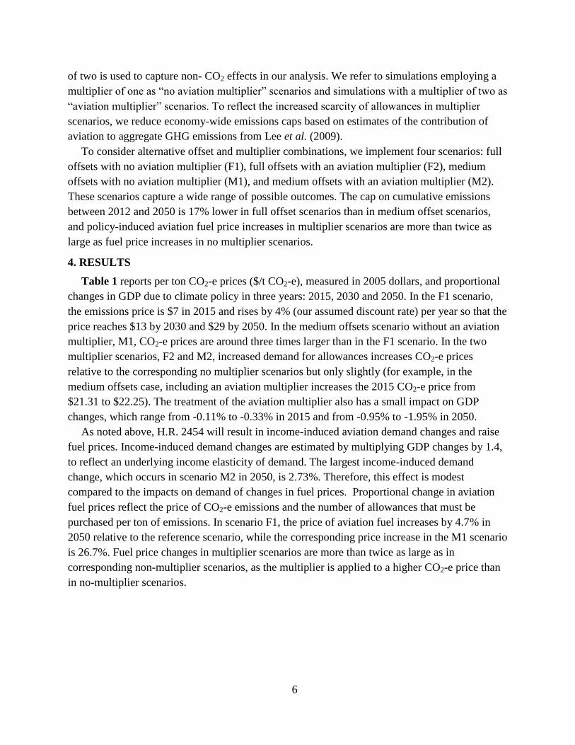
To consider alternative offset and multiplier combinations, we implement four scenarios: full

offsets with no aviation multiplier (F1), full offsets with an aviation multiplier (F2), medium

offsets with no aviation multiplier (M1), and medium offsets with an aviation multiplier (M2).

These scenarios capture a wide range of possible outcomes. The cap on cumulative emissions

between 2012 and 2050 is 17% lower in full offset scenarios than in medium offset scenarios,

and policy-induced aviation fuel price increases in multiplier scenarios are more than twice as

large as fuel price increases in no multiplier scenarios.

4. RESULTS

Table 1 reports per ton CO2-e prices ($/t CO2-e), measured in 2005 dollars, and proportional

changes in GDP due to climate policy in three years: 2015, 2030 and 2050. In the F1 scenario,

the emissions price is $7 in 2015 and rises by 4% (our assumed discount rate) per year so that the

price reaches $13 by 2030 and $29 by 2050. In the medium offsets scenario without an aviation

multiplier, M1, CO2-e prices are around three times larger than in the F1 scenario. In the two

multiplier scenarios, F2 and M2, increased demand for allowances increases CO2-e prices

relative to the corresponding no multiplier scenarios but only slightly (for example, in the

medium offsets case, including an aviation multiplier increases the 2015 CO2-e price from

$21.31 to $22.25). The treatment of the aviation multiplier also has a small impact on GDP

changes, which range from -0.11% to -0.33% in 2015 and from -0.95% to -1.95% in 2050.

As noted above, H.R. 2454 will result in income-induced aviation demand changes and raise

fuel prices. Income-induced demand changes are estimated by multiplying GDP changes by 1.4,

to reflect an underlying income elasticity of demand. The largest income-induced demand

change, which occurs in scenario M2 in 2050, is 2.73%. Therefore, this effect is modest

compared to the impacts on demand of changes in fuel prices. Proportional change in aviation

fuel prices reflect the price of CO2-e emissions and the number of allowances that must be

purchased per ton of emissions. In scenario F1, the price of aviation fuel increases by 4.7% in

2050 relative to the reference scenario, while the corresponding price increase in the M1 scenario

is 26.7%. Fuel price changes in multiplier scenarios are more than twice as large as in

corresponding non-multiplier scenarios, as the multiplier is applied to a higher CO2-e price than

in no-multiplier scenarios.

7

Table 1. U.S. CO2-e prices (in 2005 dollars) and aviation fuel price and demand changes

relative to the reference scenario.

Scenario CO2-e price

($/t CO2-e)

GDP-induced demand change (%)

Fuel price change

(%)

2015 2030 2050 2015 2030 2050 2015 2030 2050

F1 $7.27 $13.09 $28.69 -0.11% -0.43% -0.95% 5.83% 4.60% 4.74%

F2 $7.79 $14.03 $30.74 -0.12% -0.48% -1.15% 12.50% 9.20% 18.10%

M1 $21.31 $38.39 $84.07 -0.31% -1.01% -1.83% 17.50% 17.82% 26.72%

M2 $22.25 $40.07 $87.08 -0.33% -1.09% -1.95% 36.67% 41.38% 65.09%

How do changes in fuel prices influence aviation emissions and operations? Estimated annual

aviation CO2 emissions for the period 2012-2050 under our reference and four policy scenarios

are presented in Figure 1. In the reference scenario, CO2 emissions increase from 250 million

metric tons (Mt) in 2012 to 580 Mt in 2050, a 130% increase. In policy scenarios, emissions

trajectories are lower than in the reference case but absolute emissions continue to increase

substantially over the policy period, by between 97% in the most stringent scenario (M2) and

122% in the least stringent scenario (F1). Thus, airlines respond to H.R. 2454 primarily by

paying higher fuel prices rather than changing operations. This finding is consistent with other

studies of the impact of climate policy on aviation emissions (see Anger, 2010; Mendes and

Santos, 2008; Vespermann and Wald, 2010).

Three explanations emerge for the small impact of H.R. 2454 on aviation emissions. First, the

results indicate that aviation emissions mitigation options are more expensive than mitigation

operations elsewhere. This is because, as fuel costs are a significant share, around 26% (IATA,

2010), of total aviation costs, airlines already operate closer to the fuel efficiency frontier than

other industries. There is also limited scope for airlines to switch to alternative, low-emitting fuel

sources compared to industries such as electricity, where coal can be replaced by several

relatively inexpensive, low-carbon energy sources. In our EPPA simulations, the largest

proportional reduction in sectoral emissions is observed for electricity in all scenarios. In the M1

scenario, electricity emissions fall by 60% relative to reference 2050 emissions. Second, despite

large fuel price increases, demand changes induced by H.R. 2454 are small, as aviation demand

is inelastic and the policy results in modest GDP changes. Third, as detailed below, the fleet

becomes less fuel efficient in our policy scenarios than in the reference case.

8

200

250

300

350

400

450

500

550

600

650

[bill

ion

kg]

-18

-16

-14

-12

-10

-8

-6

-4

-2

0

2

% C

han

ge v

s. R

efe

ren

ce [

%]

Reference F1 F2 M1 M2

Figure 1. Aviation CO2 emissions in the reference and policy scenarios, 2006-2050.

9

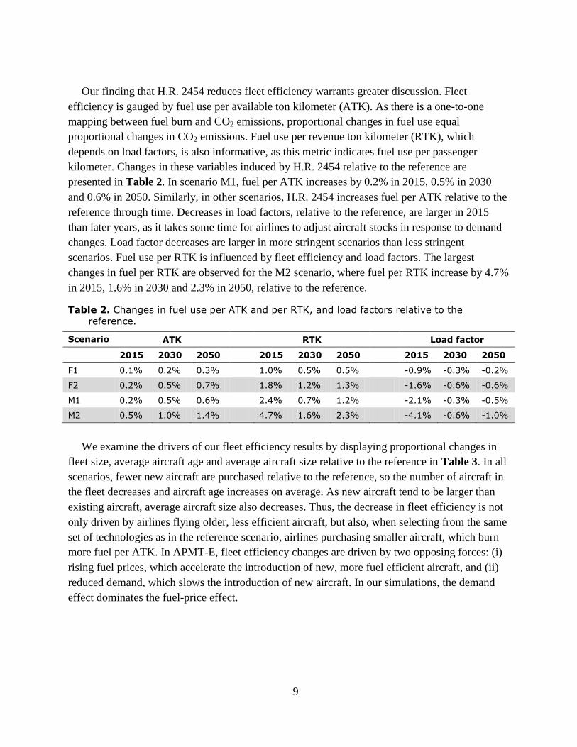
Our finding that H.R. 2454 reduces fleet efficiency warrants greater discussion. Fleet

efficiency is gauged by fuel use per available ton kilometer (ATK). As there is a one-to-one

mapping between fuel burn and CO2 emissions, proportional changes in fuel use equal

proportional changes in CO2 emissions. Fuel use per revenue ton kilometer (RTK), which

depends on load factors, is also informative, as this metric indicates fuel use per passenger

kilometer. Changes in these variables induced by H.R. 2454 relative to the reference are

presented in Table 2. In scenario M1, fuel per ATK increases by 0.2% in 2015, 0.5% in 2030

and 0.6% in 2050. Similarly, in other scenarios, H.R. 2454 increases fuel per ATK relative to the

reference through time. Decreases in load factors, relative to the reference, are larger in 2015

than later years, as it takes some time for airlines to adjust aircraft stocks in response to demand

changes. Load factor decreases are larger in more stringent scenarios than less stringent

scenarios. Fuel use per RTK is influenced by fleet efficiency and load factors. The largest

changes in fuel per RTK are observed for the M2 scenario, where fuel per RTK increase by 4.7%

in 2015, 1.6% in 2030 and 2.3% in 2050, relative to the reference.

Table 2. Changes in fuel use per ATK and per RTK, and load factors relative to the

reference.

Scenario ATK RTK Load factor

2015 2030 2050 2015 2030 2050 2015 2030 2050

F1 0.1% 0.2% 0.3% 1.0% 0.5% 0.5% -0.9% -0.3% -0.2%

F2 0.2% 0.5% 0.7% 1.8% 1.2% 1.3% -1.6% -0.6% -0.6%

M1 0.2% 0.5% 0.6% 2.4% 0.7% 1.2% -2.1% -0.3% -0.5%

M2 0.5% 1.0% 1.4% 4.7% 1.6% 2.3% -4.1% -0.6% -1.0%

We examine the drivers of our fleet efficiency results by displaying proportional changes in

fleet size, average aircraft age and average aircraft size relative to the reference in Table 3. In all

scenarios, fewer new aircraft are purchased relative to the reference, so the number of aircraft in

the fleet decreases and aircraft age increases on average. As new aircraft tend to be larger than

existing aircraft, average aircraft size also decreases. Thus, the decrease in fleet efficiency is not

only driven by airlines flying older, less efficient aircraft, but also, when selecting from the same

set of technologies as in the reference scenario, airlines purchasing smaller aircraft, which burn

more fuel per ATK. In APMT-E, fleet efficiency changes are driven by two opposing forces: (i)

rising fuel prices, which accelerate the introduction of new, more fuel efficient aircraft, and (ii)

reduced demand, which slows the introduction of new aircraft. In our simulations, the demand

effect dominates the fuel-price effect.

10

Table 3. Changes in the number of aircraft in the fleet, average aircraft age and average aircraft size relative to the reference.

Scenario Number of aircraft Average age Average size

2015 2030 2050 2015 2030 2050 2015 2030 2050

F1 -0.5% -1.9% -4.2% 0.5% 0.4% 0.8% 0.0% -0.2% -0.7%

F2 -1.2% -3.8% -8.3% 1.0% 0.8% 1.5% 0.0% -0.3% -1.1%

M1 -1.9% -4.7% -8.7% 1.5% 1.0% 1.2% 0.0% -0.1% -0.3%

M2 -3.7% -8.7% -16.0% 3.1% 1.6% 2.2% 0.0% -0.1% -0.3%

A major concern for the aviation industry is the impact of H.R. 2454 on profitability. In this

connection, the U.S. Air Transport Association (ATA) estimates that the bill would increase U.S.

airline industry costs by $5 billion in 2012 and $10 billion in 2020 (Khun, 2009). Our results are

in broad agreement with these numbers: estimated fuel cost increases range from $1.1 (F1)

billion to $6.8 billion (M2) in 2012, and from $2.7 billion (F1) to $21.4 billion (M2) in 2020.

However, cost increases in APMT-E are passed on to consumers via increased fares, so cost

increases only influence profits via their impact on demand.

To examine changes in financial viability of the aviation sector, we report changes in financial

indicators relative to the reference in Table 4. Unit (per seat mile) operating costs are affected by

rising fuel prices, decreased average efficiency, and reduced load factors. Consequently, unit

operating costs increase by 1.9% in 2015, 2.9% in 2030 and 5.0% in 2050 in scenario F1, and

larger cost increases are observed for scenarios with higher CO2-e prices. As expected, profit

changes are negatively correlated with fuel price changes. The largest proportional profit

decreases, for scenario M2, are 6.2% in 2015, 9.4% in 2030 and 17.1% in 2050, or (in 2006

dollars) $0.4 billion in 2015, $0.9 billion in 2030 and $2.9 billion in 2050.

Table 4. Changes in total operating costs, unit costs and operating profits relative to the reference.

Scenario Operating Costs Unit Costs Operating Profits

2015 2030 2050 2015 2030 2050 2015 2030 2050

F1 0.5% -0.2% -1.3% 1.9% 2.9% 5.0% -1.1% -2.5% -5.4%

F2 1.1% 1.2% 2.1% 4.0% 7.6% 15.6% -2.2% -5.0% -10.3%

M1 1.3% 0.4% -0.3% 5.5% 6.4% 11.5% -3.2% -5.0% -9.5%

M2 2.9% 3.0% 4.8% 11.5% 15.3% 29.8% -6.2% -9.4% -17.1%

5. SENSITIVITY ANALYSIS

An important finding in our analysis is that H.R. 2454 reduces fleet efficiency. In this section,

we investigate the robustness of this result to key components of AMPT-E. Specifically, we

examine the sensitivity of results to aircraft retirement decisions, aircraft fuel-efficiency

improvements, and income and price elasticities. As above, proportional changes in fuel use per

ATK relative to the reference scenario are used to measure efficiency changes. Table 5 reports

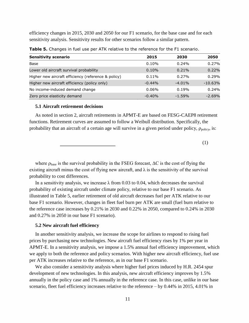
11

efficiency changes in 2015, 2030 and 2050 for our F1 scenario, for the base case and for each

sensitivity analysis. Sensitivity results for other scenarios follow a similar pattern.

Table 5. Changes in fuel use per ATK relative to the reference for the F1 scenario.

Sensitivity scenario 2015 2030 2050

Base 0.10% 0.24% 0.27%

Lower old aircraft survival probability 0.10% 0.21% 0.22%

Higher new aircraft efficiency (reference & policy) 0.11% 0.27% 0.29%

Higher new aircraft efficiency (policy only) -0.44% -4.01% -10.63%

No income-induced demand change 0.06% 0.19% 0.24%

Zero price elasticity demand -0.40% -1.59% -2.69%

5.1 Aircraft retirement decisions

As noted in section 2, aircraft retirements in APMT-E are based on FESG-CAEP8 retirement

functions. Retirement curves are assumed to follow a Weibull distribution. Specifically, the

probability that an aircraft of a certain age will survive in a given period under policy, ρpolicy, is:

(1)

where ρbase is the survival probability in the FSEG forecast, ΔC is the cost of flying the

existing aircraft minus the cost of flying new aircraft, and λ is the sensitivity of the survival

probability to cost differences.

In a sensitivity analysis, we increase λ from 0.03 to 0.04, which decreases the survival

probability of existing aircraft under climate policy, relative to our base F1 scenario. As

illustrated in Table 5, earlier retirement of old aircraft decreases fuel per ATK relative to our

base F1 scenario. However, changes in fleet fuel burn per ATK are small (fuel burn relative to

the reference case increases by 0.21% in 2030 and 0.22% in 2050, compared to 0.24% in 2030

and 0.27% in 2050 in our base F1 scenario).

5.2 New aircraft fuel efficiency

In another sensitivity analysis, we increase the scope for airlines to respond to rising fuel

prices by purchasing new technologies. New aircraft fuel efficiency rises by 1% per year in

APMT-E. In a sensitivity analysis, we impose a 1.5% annual fuel efficiency improvement, which

we apply to both the reference and policy scenarios. With higher new aircraft efficiency, fuel use

per ATK increases relative to the reference, as in our base F1 scenario.

We also consider a sensitivity analysis where higher fuel prices induced by H.R. 2454 spur

development of new technologies. In this analysis, new aircraft efficiency improves by 1.5%

annually in the policy case and 1% annually in the reference case. In this case, unlike in our base

scenario, fleet fuel efficiency increases relative to the reference – by 0.44% in 2015, 4.01% in

12

2030, and 10.63% in 2050. These efficiency changes are large, but not unexpected given that the

growth rate for new aircraft efficiency is 50% larger in the policy scenario than in the reference.

This simulation indicates the importance of technology responses to price changes.

5.3 Income and price elasticities

H.R. 2454 slows the introduction of new aircraft by reducing the demand for aviation.

Accordingly, in separate sensitivity analyses, we examine the impact of the income elasticity of

demand and price elasticities of demand. In one analysis, we set the income elasticity of demand

for aviation equal to zero, so GDP changes induced by climate policy do not influence aviation

demand. Under such a scenario, fuel per ATK decreases relative to the base F1 scenario, but still

increases relative to the reference scenario, by 0.24% in 2050. In another analysis, we set the

price elasticity of demand for aviation equal to zero. Under this extreme price-response

assumption, fuel use per ATK, relative to the reference, decreases by 0.40% in 2015, 1.59% in

2030 and 2.69% in 2050.

6. CONCLUSIONS

We examined the impact of climate policy on aviation emissions and economic outcomes in

the U.S.. Our analysis, benchmarked to ICAO/GIACC (2009) forecasts, estimated that aviation

emissions between 2012 and 2050 will increase by between 97% and 122% under H.R.2454,

compared to 130% without climate policy. These results indicate that aviation emissions

abatement options are costly relative to mitigation options in other sectors. Key determinants of

marginal abatement costs in APMT-E include the specification of new aircraft capital costs, fuel

efficiency improvements, and retirement rates. Currently, there are limited opportunities for

airlines to replace more CO2-intensive energy sources with less CO2-intensive energy sources,

and to substitute between energy and other inputs.

Another noteworthy finding is that, under the set of assumptions in our framework, GDP and

fuel price changes induced by H.R. 2454 reduce fleet efficiency, as the demand effect

outweighed the fuel-price effect. That is, the impact of reduced demand for aviation on new

aircraft purchase decisions dominated incentives to purchase more efficient aircraft in the face of

rising fuel prices. We examined the sensitivity of our results to several key modeling

assumptions. In general, our finding that H.R. 2454 reduces average fleet efficiency is robust to

plausible alternative modeling assumptions examined in our sensitivity analyses. However, our

fleet efficiency results were overturned when we assumed that aviation demand was perfectly

inelastic, and when we assumed that fuel price increases induced by H.R 2454 increased the fuel

efficiency of new aircraft by 50%, relative to the reference scenario.

Several caveats to our analysis should be noted. First, as we focused on long-run trends,

adjustments associated with business cycles were not considered. In economic downturns,

airlines may park old aircraft, which are replaced by new aircraft in high-growth periods rather

than brought back into service. Second, our modeling framework did not capture some

adjustments available to airlines using the existing fleet. For example, we did not allow airlines

to retrofit seat configurations or use slower flight speeds in response to fuel price changes. Third,

13

we did not consider how changes in air traffic management, induced by climate policy, might

improve operations and reduce emissions. When these adjustments are considered, climate

policy may have a larger positive impact on fleet efficiency than in our study. Future research

will focus on this.

Acknowledgments

The authors would like to thank Thomas Cuddy, Maryaclie Locke, Richard Hancox, Caroline

Sinclair, Carl Tipton and Daniel Rankin for valuable input. Any errors are the sole responsibility

of the authors. This work is funded by the U.S. Federal Aviation Administration Office of

Environment and Energy under FAA Award Number: 06-C-NE-MIT, Amendment Nos. 018 and

028. The project is managed by Thomas Cuddy of FAA. The Joint Program on the Science and

Policy of Global Change is funded by the U.S. Department of Energy and a consortium of

government and industrial sponsors (for a complete list, see

http://globalchange.mit.edu/sponsors/current.html). Additional funding for Wollersheim was

provided by the Erich-Becker Foundation. Any opinions, findings, and conclusions or

recommendations expressed in this material are those of the authors and do not necessarily

reflect the views of the FAA, NASA or Transport Canada. This report is also released as

Partnership for AiR Transportation Noise and Emissions Reduction (PARTNER) Report No.

PARTNER-COE-2011-001.

7. REFERENCES

Airbus, 2009: Flying smart, thinking big, Global Market Forecast 2009-2028, Blagnac Cedex.

Albers, S., J.A. Bühne, and H. Peters, 2009: Will the EU-ETS instigate airline network

reconfigurations? Journal of Air Transport Management, 15(1): 1-6.

Anger, A., and J. Köhler, 2010: Including aviation emissions in the EU ETS: Much ado about

nothing? A review. Transport Policy, 17(2): 38-46.

Boeing, 2010: Current Market Outlook 2009-2028. (http://active.boeing.com/commercial/

forecast_data/index.cfm).

Bond, T.C., D.G. Streets, K.F. Yarber, S.M. Nelson and J. Woo, 2004: A technology-based

global inventory of black and organic carbon emissions from combustion. Journal of

Geophysical Research, 109: D14203.

Boon, B., M. Davidson, J. Faber and A. van Velzen, 2007: Allocation of allowances for aviation

in the EU ETS – The impact on the profitability of the aviation sector under high levels of

auctioning. A report for WWF UK, Delft, CE Delft, March 2007.

Clarke, L., J. Edmonds, V. Krey, R. Richels, M. Tavoni and S. Rose 2009: International climate

policy architectures: Overview of the EMF 22 international scenarios. Energy Economics,

31(S2): S64-S81.

Dimaranan, B.V. (ed.) 2006: Global Trade, Assistance, and Production: The GTAP 6 Data Base.

Center for Global Trade Analysis, Purdue University.

Ernst and Young, 2007: Analysis of the EC proposal to include aviation activities in the

Emissions Trading Scheme, A report by Ernst and Young and York Aviation, York.

Forsyth, P., 2008: The impact of climate change policy on competition in the air transport

industry. Department of Economics, Monash University, Discussion paper No. 2008-18.

14

Gillen, D.W., W.G. Morrison and C. Stewart, 2002: Air travel demand elasticities: Concepts,

issues and measurement, Final Report, Department of Finance, Canada.

Haites, E., 2009: Linking emissions trading schemes for international aviation and shipping

emissions. Climate Policy, 9(4): 415-430.

Hofer, C., M.E. Dresner, and R.J. Windle, 2010: The environmental effects of airline carbon

emissions taxation in the U.S.. Transportation Research Part D (Transport and

Environment), 15: 37-45.

IATA (International Air Transport Association) 2010: Fuel impact on operating costs

(https://www.iata.org/pressroom/facts_figures/fact_sheets/Pages/fuel.aspx).

ICAO/GIACC (International Civil Aviation Organization / Group on International Aviation and

Climate Change), 2009: U.S. fuel trends analysis and comparison to GIACC/4-IP/1, Fourth

Meeting of the Group on International Aviation and Climate Change, May 25 to 28, 2009,

Montreal.

IEA (International Energy Agency), 2004: World Energy Outlook: 2004. OECD/IEA: Paris.

Khun, M., 2009: U.S. cap and trade scheme could cost billions: ATA, FlightGlobe, Sutton, UK.

(http://www.flightglobal.com/articles/2009/05/28/327041/us-cap-and-trade-scheme-could-

cost-billions-ata.html).

Kincaid, I. and M. Tretheway, 2007: Estimating air travel demand elasticities, InterVISTAS.

Lee D.S., D. Pitari, V. Grewe, K. Gierens, J.E. Penner, A. Petzold, M.J. Prather, U. Schumann,

A. Bais, T. Bernsten, D. lachetti, L.L. Lim, R. Sausen, 2009: Transport impacts on

atmosphere and climate: Aviation, Atmospheric Environment, In Press.

(doi:10.1016/j.atmosenv.2009.06.005).

Mahashabde, A., P. Wolfe, A. Ashok, C. Dorbian, Q. He, A. Fan, S. Lukachko, A.

Mozdzanowska, C. Wollersheim, S. Barrett, M. Locke, and I. A. Waitz, 2010: Assessing the

environmental impacts of aircraft noise and emissions. Progress in Aerospace Sciences, in

Press.

Mayor, K. and R.S.J. Tol, 2010: The impact of European climate change regulations on

international tourist markets. Transportation Research Part D (Transport and Environment),

15: 26-36.

Mendes, L.M.Z. and Santos, 2008: Using economic instruments to address emissions from air

transport in the European Union. Environment and Planning A, 40(1): 189-209.

Morrell, P., 2007: An evaluation of possible EU air transport emissions trading scheme

allocation methods. Energy Policy, 35: 5562-5570.

MVA Consultancy, 2009: Aviation Environmental Portfolio Management Tool (APMT):

APMT-Economics. Algorithm Design Document (ADD), MVA Consultancy, London and

Manchester.

Oberthür, S., 2003: Institutional interaction to address greenhouse gas emissions from

international transport: ICAO, IMO and the Kyoto Protocol. Climate Policy, 3: 191-205.

Olivier, J.G.J. and J.J.M. Berdowski, 2001: Global emissions sources and sinks. In: The Climate

System, J. Berdowski, R. Guicherit and B.J. Heij (eds.), A.A. Balkema Publishers/Swets &

Zeitlinger Publishers, Lisse, The Netherlands, pp. 33-78.

Paltsev, S., J. Reilly, H.D. Jacoby, R.S. Eckaus, J. McFarland, M. Sarofim, M. Asadooria and M.

Babiker, 2005: The MIT Emissions Prediction and Policy Analysis (EPPA) Model: Version

15

4. MIT JPSPGC Report 125, August, 72 p.

(http://globalchange.mit.edu/files/document/MITJPSPGC_Rpt125.pdf).

Paltsev S., J. Reilly, H. Jacoby, A. Gurgel, G. Metcalf, A. Sokolov and J. Holak, 2007:

Assessment of U.S. cap-and-trade proposals. Climate Policy, 8(4): 395-420; MIT Joint

Program Reprint 2008-16;

http://globalchange.mit.edu/files/document/MITJPSPGC_Reprint08-16.pdf.

Paltsev S., J. Reilly, H. Jacoby, and J. Morris, 2009: The cost of climate policy in the United

States. Energy Economics, 31(S2): S235-S243; MIT Joint Program Reprint 2009-16;

http://globalchange.mit.edu/pubs/abstract.php?publication_id=2020.

Penner J.E., D.H. Lister, D.J. Griggs, D.J. Dokken and M. McFarland, 1999: Aviation and the

Global Atmosphere: A Special Report of IPCC Working Groups I and III, Intergovernmental

Panel on Climate Change, Cambridge University Press, Cambridge/New York.

Petersen, M., 2008: The legality of the EU’s stand-alone approach to the climate impact of

aviation: the express role given to the ICAO by the Kyoto protocol. Review of European

Community and International Environmental Law, 17(2): 196-204.

Scheelhaase, J.D., and W.G. Grimme, 2007: Emissions trading for international aviation – an

estimation of the economic impact on selected European airlines. Journal of Air Transport

Management, 13(5): 253-263.

Scheelhaase, J.D., M. Schaefer, W.G. Grimme and S. Maertens, 2010: The inclusion of aviation

into the EU emission trading scheme – Impacts on competition between European and non-

European network airlines. Transportation Research Part D (Transport and Environment),

15(1): 14-25.

Vespermann, J. and A. Wald, 2010: Much ado about nothing? – An analysis of economic

impacts and ecologic effects of the EU-emissions trading scheme in the aviation industry.

Transportation Research Part A, in press.

Wit, R.C.N., B.H. Boon, A. van Velzen, M. Cames, O. Deuber, and D.S. Lee, 2005: Giving

wings to emission trading – Inclusion of aviation under the European emission trading

system (ETS): Design and impacts, CE Solutions for Environment, Economic and

Technology, Report for the European Commission, Delft.

16

APPENDIX: LITERATURE REVIEW

Several studies examine the impact of climate policy on aviation. To date, most papers focus

on the EU-ETS. Some studies analyze the general implications of cap-and-trade schemes or

carbon taxes. To our knowledge, only one study, Hofer et al. (2010), focuses on U.S. Table A1

summarizes the literature to date. Studies can be grouped into three categories: (1) papers

focusing on aviation financial indicators and environmental benefits from reduced aviation

emissions, (2) analyses of the competitive effects of carbon policies, and (3) studies that analyze

legal and political aspects. Studies focusing on legal aspects include Haites (2009), Oberthuer

(2003), and Peterson (2008). Studies examining the impact of climate policy on airline

competition tend to analyze case studies (Albers et al., 2009; Forsyth, 2008; and Scheelhaase et

al., 2010). Papers that assess the financial and environmental implications of including aviation

in climate policy either utilize existing models (Anger, 2010; Boon et al., 2007; and Wit et al,

2005) or develop new models (Ernst and Young, 2007, Hofer et al., 2010; Mendes, 2008,

Morrell, 2007, Scheelhaase and Grimme, 2007; Vespermann, and Wald, 2010). All studies in

this group use an assumed allowance price, except Anger (2010), who uses a dynamic

macroeconomic model.

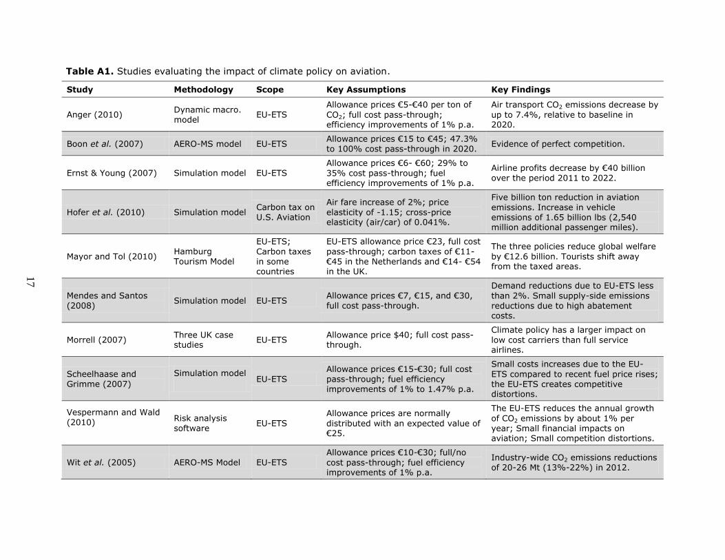
Table A1. Studies evaluating the impact of climate policy on aviation.

Study Methodology Scope Key Assumptions Key Findings

Anger (2010) Dynamic macro. model

EU-ETS Allowance prices €5-€40 per ton of

CO2; full cost pass-through; efficiency improvements of 1% p.a.

Air transport CO2 emissions decrease by

up to 7.4%, relative to baseline in 2020.

Boon et al. (2007) AERO-MS model EU-ETS Allowance prices €15 to €45; 47.3% to 100% cost pass-through in 2020.

Evidence of perfect competition.

Ernst & Young (2007) Simulation model EU-ETS Allowance prices €6- €60; 29% to

35% cost pass-through; fuel efficiency improvements of 1% p.a.

Airline profits decrease by €40 billion over the period 2011 to 2022.

Hofer et al. (2010) Simulation model Carbon tax on U.S. Aviation

Air fare increase of 2%; price

elasticity of -1.15; cross-price elasticity (air/car) of 0.041%.

Five billion ton reduction in aviation

emissions. Increase in vehicle emissions of 1.65 billion lbs (2,540 million additional passenger miles).

Mayor and Tol (2010) Hamburg Tourism Model

EU-ETS;

Carbon taxes in some countries

EU-ETS allowance price €23, full cost

pass-through; carbon taxes of €11-€45 in the Netherlands and €14- €54 in the UK.

The three policies reduce global welfare

by €12.6 billion. Tourists shift away from the taxed areas.

Mendes and Santos

(2008) Simulation model EU-ETS

Allowance prices €7, €15, and €30,

full cost pass-through.

Demand reductions due to EU-ETS less

than 2%. Small supply-side emissions

reductions due to high abatement costs.

Morrell (2007) Three UK case studies

EU-ETS Allowance price $40; full cost pass-through.

Climate policy has a larger impact on

low cost carriers than full service airlines.

Scheelhaase and Grimme (2007)

Simulation model

EU-ETS

Allowance prices €15-€30; full cost pass-through; fuel efficiency improvements of 1% to 1.47% p.a.

Small costs increases due to the EU-

ETS compared to recent fuel price rises; the EU-ETS creates competitive distortions.

Vespermann and Wald

(2010)

Risk analysis

software EU-ETS

Allowance prices are normally

distributed with an expected value of €25.

The EU-ETS reduces the annual growth

of CO2 emissions by about 1% per

year; Small financial impacts on aviation; Small competition distortions.

Wit et al. (2005) AERO-MS Model EU-ETS Allowance prices €10-€30; full/no

cost pass-through; fuel efficiency improvements of 1% p.a.

Industry-wide CO2 emissions reductions of 20-26 Mt (13%-22%) in 2012.

17