IPN Progress Report 42-155 November 15, 2003

The ICER Progressive Wavelet Image CompressorA. Kiely1 and M. Klimesh1

ICER is a progressive, wavelet-based image data compressor designed to meetthe specialized needs of deep-space applications while achieving state-of-the-artcompression effectiveness. ICER can provide lossless and lossy compression, andincorporates an error-containment scheme to limit the effects of data loss duringtransmission. The Mars Exploration Rover (MER) mission will rely primarily ona software implementation of ICER for image compression. This article describesICER and the methods it uses to meet its goals, and explains the rationale behindthe choice of methods. Performance results also are presented.

I. Introduction

In early 2004, the Mars Exploration Rover (MER) mission will land a pair of rovers on Mars. Wellover half of the bits transmitted from the rovers will consist of compressed image data gathered fromthe unprecedented nine cameras onboard each rover. The MER rovers will rely exclusively on the ICERimage compressor for all lossy image compression.

ICER is a wavelet-based image compressor designed for use with the deep-space channel. The de-velopment of ICER was driven by the desire to achieve state-of-the-art compression performance withsoftware that meets the specialized needs of deep-space applications. ICER features progressive compres-sion and by nature can provide both lossless and lossy compression. ICER incorporates a sophisticatederror-containment scheme to limit the effects of data losses seen on the deep-space channel.

In this article, we describe ICER and the methods it uses to meet its goals, and explain the rationalebehind the choice of methods. We start with an overview of ICER’s features and the techniques ICERuses.

A. Progressive Compression

Under a progressive data compression scheme, compressed information is organized so that as more ofthe compressed data stream is received, reconstructed images of successively higher overall quality can bereproduced. Figure 1 illustrates this increase in quality for an example image, as a function of the resultingeffective bit rate. Truncating a progressively compressed data stream by increasing amounts produces agraceful degradation in the reconstructed image quality. Thus, progressive compression provides a simpleand effective method of meeting a constraint on compressed data volume without the need to guess at anappropriate setting of an image-quality parameter.

1 Communications Systems and Research Section.

The research described in this publication was carried out by the Jet Propulsion Laboratory, California Institute ofTechnology, under a contract with the National Aeronautics and Space Administration.

1

Fig. 1. This sequence of image details from a larger image shows how overall image quality improves under progressive compression as more compressed data are received: (a) 0.125 bits/pixel, (b) 0.25 bits/pixel, (c) 0.5 bits/pixel, and (d) 1 bit/pixel.

(a) (b) (c) (d)

By contrast, non-progressive compression techniques typically encode information one region at atime (where a region may be a pixel or a small block of pixels), gradually covering the image spatially.Truncating the data stream produced by a non-progressive algorithm generally results in complete lossof information for some portion of the image.

Using ICER, one could send a small fraction of the data from a compressed image to get a low-quality preview, and later send more of the data to get a higher-quality version if the image is deemedinteresting. In future missions, progressive compression will enable sophisticated data-return strategiesinvolving incremental image-quality improvements to maximize the science value of returned data usingan onboard buffer [1].

B. How ICER Works: An Overview

The first step in wavelet-based image compression is to apply a wavelet transform to the image. Awavelet transform is a linear (or nearly linear) transform designed to decorrelate images by local separationof spatial frequencies. The transform decomposes the image into several subbands, each a smaller versionof the image, but filtered to contain a limited range of spatial frequencies.

The wavelet transforms used by ICER are described in Section II. An ICER user can select one of seveninteger wavelet transforms and can control the number of subbands by choosing the number of stages ofwavelet decomposition applied to the image. The wavelet transforms used by ICER are invertible; thus,image compression is lossless when all of the compressed subband data are losslessly encoded.

By using a wavelet transform, ICER avoids the “blocking” artifacts that can occur when the discretecosine transform (DCT) is used for decorrelation, as in the Joint Photographic Experts Group (JPEG)compressor used on the Mars Pathfinder mission. The wavelet compression of ICER does introduce“ringing” artifacts (spurious faint oscillations or edges, usually near sharp edges in the image), but thesetend to be less objectionable. Both types of artifacts are illustrated in Fig. 2. In addition to producing lessnoticeable artifacts, wavelet-based compression is usually superior to DCT-based compression in termsof quantitative measures of reconstructed image quality.

Following the wavelet transform, ICER compresses a simple binary representation of the transformedimage, achieving progressive compression by successively encoding groups of bits, starting with groupscontaining highly significant bits and working toward groups containing less significant bits. During thisencoding process, ICER maintains a statistical model that is used to estimate the probability that thenext bit to be encoded is a zero. ICER’s method of modeling the image is a form of context modeling.This and other details of the encoding procedure are described in Section III. The probability estimatesproduced by the context modeler are used by an entropy coder to compress the sequence of bits. ICER’sentropy coder is described in Section IV.

2

(a) (b) (c)

Fig. 2. Details from a larger image: (a) original image, (b) reconstructed image illustrating ringing artifacts after compression to 0.125 bits/pixel using ICER, and (c) reconstructed image illustrating blocking artifacts after compression to 0.178 bits/pixel using JPEG. In this example, the ringing artifacts under ICER are less noticeable than the blocking artifacts under JPEG, even though the image is more highly compressed under ICER.

For error-containment purposes, the wavelet-transformed image is partitioned into a user-selectablenumber of segments, each roughly corresponding to a rectangular portion of the image. Data within eachsegment are compressed independently of the others so that if data pertaining to a segment are lost orcorrupted, the other segments are unaffected. Increasing the number of segments (and thus reducing theirsize) helps to contain the effects of a packet loss to a smaller region of the image; however, it’s generallyharder to effectively compress smaller segments. By varying the number of segments, a user can controlthis trade-off between compression effectiveness and robustness to data loss, allowing some adaptabilityto different data loss statistics. Section V discusses error and loss mechanisms of the deep-space channeland ICER’s error-containment process in more detail.

Image quality and the amount of compression are primarily controlled by two parameters: a bytequota, which controls the maximum number of compressed bytes produced, and a quality goal parameterthat tells ICER to stop producing compressed bytes when a simple image-quality criterion is met. ICERstops once the quality goal or byte quota is met, whichever comes first. Section VI contains a detaileddiscussion of the byte quota and quality goal parameters, as well as related issues.

Section VII gives results comparing ICER’s compression effectiveness to that of other compressors.

C. ICER on MER

The first space use of ICER will be on the MER mission, which will rely on a software implementationof ICER for all lossy image compression. Each MER rover will operate for 90 Martian days and willcollect image data using nine visible-wavelength cameras: a mast-mounted, high-angular-resolution colorimager for science investigations (the panoramic camera, or Pancam); a mast-mounted, medium-angular-resolution camera for navigation purposes (the Navcam); a set of body-mounted front and rear camerasfor navigation hazard avoidance (the Hazcams); and a high-spatial-resolution camera (the MicroscopicImager) mounted on the end of a robotic arm for science investigations. With the exception of theMicroscopic Imager, all of these cameras are actually stereo camera pairs. Not surprisingly, collectingand transmitting images to Earth will be a major priority of the mission.

All MER cameras produce 1024-pixel by 1024-pixel images at 12 bits per pixel. Images transmittedfrom MER will range from tiny 64 × 64 “thumbnail” images, up to full-size images. Current plans callfor navigation, thumbnail, and many other image types to be compressed to approximately 1 bit/pixel,and lower bit rates (less than 0.5 bit/pixel) will be used for certain wavelengths of multi-color panoramicimages. At the other end of the compression spectrum, radiometric calibration targets are likely to becompressed to about 4 to 6 bits/pixel [2]. When stereo image pairs are compressed, each image in thepair is compressed independently.

3

Lossless compression will be used when maximum geometric and radiometric fidelity is required, but inthis case MER generally will use the LOCO (Low Complexity Lossless Compression) image compressor[3–5], which, because it is dedicated solely to lossless compression, is able to provide faster losslesscompression than ICER with comparable compression effectiveness (see Section VII).

As we’ll see in Section VII, ICER delivers state-of-the-art image compression effectiveness, significantlyimproving on the compressors used by the Mars Pathfinder mission. ICER’s compression effectivenesswill enhance the ability of the MER mission to meet its science objectives.2

II. Wavelet Transform

The first step in ICER compression is to perform a two-dimensional wavelet transform to decomposethe image into a user-controlled number of subbands. Each stage of the two-dimensional wavelet decom-position is accomplished by applying a one-dimensional wavelet transform to rows and columns of data.The wavelet transform is used to decorrelate the image, concentrating most of the important informationinto a small number of small subbands. Thus, a good approximation to the original image can be obtainedfrom a small amount of data. In addition, the subbands containing little information tend to compresseasily. The wavelet transform does leave some correlation in the subbands, so compression of the subbanddata uses the predictive compression method described in Section III to attempt to exploit as much ofthis remaining correlation as possible.

A. One-Dimensional Wavelet Transform

Performing a one-dimensional wavelet transform on a data sequence amounts to applying a high-pass/low-pass filter pair to the sequence and downsampling the results by a factor of 2. The transformmethod used by ICER is from [6,7], although we use slightly different notation in our description.

We are specifically interested in reversible integer wavelet transforms. That is, we want a wavelettransform that produces integer outputs and that is exactly invertible when the input consists of integers.This allows us to achieve lossless compression when all of the transformed data are reproduced exactly.3

Fortunately, other researchers have considered the problem of finding good reversible integer wavelettransforms; several are tabulated in [9].

An ICER user can select one of seven reversible integer wavelet transforms that are all computed inessentially the same way, but which use different choices of filter coefficients. These wavelet transformsare nonlinear approximations to linear high-pass/low-pass filter pairs. The nonlinearity arises from theuse of roundoff operations.

We begin with a length-N (N ≥ 3) data sequence x[n], n = 0, 1, · · · , N−1. A wavelet transform of thissequence produces �N/2� low-pass outputs �[n], n = 0, 1, · · · , �N/2� − 1, and �N/2� high-pass outputsh[n], n = 0, 1, · · · , �N/2� − 1. Thus, the total number of outputs from the wavelet transform is equal tothe number of data samples.

2 For more information on the usage, implementation, and operational details of the the ICER software used by MER, werefer the reader to A. Kiely and M. Klimesh, Mars Exploration Rover (MER) Project ICER User’s Guide, JPL D-22103,MER 420-8-538 (internal document), Jet Propulsion Laboratory, Pasadena, California, December 13, 2001, which explainsdetails such as the organization of compressed data in the encoded bitstream, limits on allowed values of ICER parameters,and input/output interfaces.

3 It is easy to construct integer wavelet transforms that are reversible but not well suited to data compression. For example,one could use a linear filter pair with integer coefficients that have large magnitude, thus producing output with a largedynamic range. In this case, there would be a lot of bits to encode, and the least-significant bits would contain a substantialamount of redundancy; hence, the transform would not be convenient for lossless or near-lossless data compression. Weare really interested in efficient reversible transforms; see [8, p. 214] for a discussion.

4

The low-pass outputs �[n], n = 0, 1, · · · , �N/2� − 1 are given by

�[n] =

⎧⎪⎪⎪⎨⎪⎪⎪⎩

⌊12(x[2n] + x[2n + 1]

)⌋, n = 0, 1, · · · ,

⌊N

2

⌋− 1

x[N − 1], n =N − 1

2, N odd

The low-pass filter used for each of the wavelet transforms is the same, and essentially takes averages ofadjacent data samples.

To compute the high-pass outputs, for n = 0, 1, · · · , �N/2� − 1 we first compute

d[n] =

⎧⎪⎪⎪⎨⎪⎪⎪⎩

x[2n] − x[2n + 1], n = 0, 1, · · · ,⌊

N

2

⌋− 1

0, n =N − 1

2, N odd

(1)

and

r[n] = �[n − 1] − �[n], n = 1, 2, · · · ,⌈

N

2

⌉− 1 (2)

Then for n = 0, 1, · · · , �N/2� − 1, the high-pass outputs h[n] are computed as

h[n] = d[n] −

⎧⎪⎪⎪⎪⎪⎪⎪⎪⎪⎪⎪⎪⎪⎪⎨⎪⎪⎪⎪⎪⎪⎪⎪⎪⎪⎪⎪⎪⎪⎩

⌊14r[1]

⌋, n = 0

⌊14r[1] +

38r[2] − 1

4d[2] +

12

⌋, n = 1, α−1 �= 0

⌊14r

[N

2− 1

]⌋, N even, n = N/2 − 1

⌊α−1r[n − 1] + α0r[n] + α1r[n + 1] − βd[n + 1] +

12

⌋, otherwise

(3)

Table 1 gives the filter parameters α−1, α0, α1, β for each of the filters used by ICER. Filter Q wasdevised by the first author of this article; the others are from [6,7]. Filter A is also essentially the sameas the “Reversible Two-Six” transform in [8]; the only differences are in the way roundoff operations areperformed.

The high-pass filter outputs h[n] are approximately equal to the following linear filter outputs:

h[n] =3∑

i=−4

cix[2n + i] (4)

5

where the filter coefficients are

(c−4,c−3, c−2, c−1, c0, c1, c2, c3) =

12(−α−1,−α−1, α−1 − α0, α−1 − α0, 2 + α0 − α1,−(2 − α0 + α1), α1 + 2β, α1 − 2β) (5)

Table 2 lists the values of these coefficients for each filter. For each filter, it can be shown that thedifference between the exact and approximate high-pass filter output is bounded as follows:

|h[n] − h[n]| ≤ 12

+14

(|α−1| + |α0 − α−1| + |α1 − α0| + |α1|) ≤2532

(6)

To invert the transform given the high-pass outputs h[n] and low-pass outputs �[n], we first compute thevalues of r[n] using Eq. (2). Then we compute the values of d[n] by inverting Eq. (3). This computationis done in order of decreasing index n.4 Finally, we recover the original data sequence x[n] using

x[2n] = �[n] +⌊

d[n] + 12

⌋

x[2n + 1] = x[2n] − d[n]

Reversible integer wavelet transforms such as the ones described here also can be computed using the“lifting” technique; see [9] for a good summary. Both methods require the same number of arithmeticoperations. Note that roundoff operations in the transforms of [9] are done in a slightly different way;consequently, the inverse transforms are also different.

Table 1. Wavelet filter parameters.

Filter α−1 α0 α1 β

A 0 1/4 1/4 0

B 0 2/8 3/8 2/8

C −1/16 4/16 8/16 6/16

D 0 4/16 5/16 2/16

E 0 3/16 8/16 6/16

F 0 3/16 9/16 8/16

Q 0 1/4 1/4 1/4

4 To begin calculating the sequence of d[n] values, when N is even, note from Eq. (3) that d[(N/2) − 1] = h[(N/2) − 1] +�(1/4)r[(N/2) − 1]�, and when N is odd, note from Eq. (1) that d[(N − 1)/2] = 0.

6

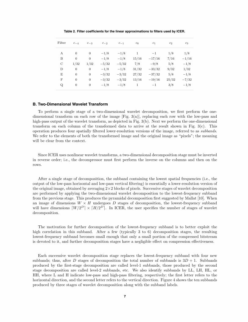
Table 2. Filter coefficients for the linear approximations to filters used by ICER.

Filter c−4 c−3 c−2 c−1 c0 c1 c2 c3

A 0 0 −1/8 −1/8 1 −1 1/8 1/8

B 0 0 −1/8 −1/8 15/16 −17/16 7/16 −1/16

C 1/32 1/32 −5/32 −5/32 7/8 −9/8 5/8 −1/8

D 0 0 −1/8 −1/8 31/32 −33/32 9/32 1/32

E 0 0 −3/32 −3/32 27/32 −37/32 5/8 −1/8

F 0 0 −3/32 −3/32 13/16 −19/16 25/32 −7/32

Q 0 0 −1/8 −1/8 1 −1 3/8 −1/8

B. Two-Dimensional Wavelet Transform

To perform a single stage of a two-dimensional wavelet decomposition, we first perform the one-dimensional transform on each row of the image [Fig. 3(a)], replacing each row with the low-pass andhigh-pass output of the wavelet transform, as depicted in Fig. 3(b). Next we perform the one-dimensionaltransform on each column of the transformed data to arrive at the result shown in Fig. 3(c). Thisoperation produces four spatially filtered lower-resolution versions of the image, referred to as subbands.We refer to the elements of both the transformed image and the original image as “pixels”; the meaningwill be clear from the context.

Since ICER uses nonlinear wavelet transforms, a two-dimensional decomposition stage must be invertedin reverse order; i.e., the decompressor must first perform the inverse on the columns and then on therows.

After a single stage of decomposition, the subband containing the lowest spatial frequencies (i.e., theoutput of the low-pass horizontal and low-pass vertical filtering) is essentially a lower-resolution version ofthe original image, obtained by averaging 2×2 blocks of pixels. Successive stages of wavelet decompositionare performed by applying the two-dimensional wavelet decomposition to the lowest-frequency subbandfrom the previous stage. This produces the pyramidal decomposition first suggested by Mallat [10]. Whenan image of dimensions W × H undergoes D stages of decomposition, the lowest-frequency subbandwill have dimensions �W/2D� × �H/2D�. In ICER, the user specifies the number of stages of waveletdecomposition.

The motivation for further decomposition of the lowest-frequency subband is to better exploit thehigh correlation in this subband. After a few (typically 3 to 6) decomposition stages, the resultinglowest-frequency subband becomes small enough that only a small portion of the compressed bitstreamis devoted to it, and further decomposition stages have a negligible effect on compression effectiveness.

Each successive wavelet decomposition stage replaces the lowest-frequency subband with four newsubbands; thus, after D stages of decomposition the total number of subbands is 3D + 1. Subbandsproduced by the first-stage decomposition are called level-1 subbands, those produced by the secondstage decomposition are called level-2 subbands, etc. We also identify subbands by LL, LH, HL, orHH, where L and H indicate low-pass and high-pass filtering, respectively; the first letter refers to thehorizontal direction, and the second letter refers to the vertical direction. Figure 4 shows the ten subbandsproduced by three stages of wavelet decomposition along with the subband labels.

7

Original Image

Horizontal Low-Pass

Horizontal High-Pass

Horizontal Low-Pass,

Vertical Low-Pass

Horizontal High-Pass,

Vertical Low-Pass

Horizontal Low-Pass,

Vertical High-Pass

Horizontal High-Pass,

Vertical High-Pass

Fig. 3. One stage of a two-dimensional wavelet decomposition: (a) original image, (b) horizontal decomposition of the image, and (c) two-dimensional decomposition of the image. Pixel magnitudes are shown, and the image is contrast enhanced (magnitudes scaled by a factor of 6) in the subbands that have been high-pass filtered.

(a) (b) (c)

LL HL

HHLHHL

Level-2 Level-1

HHLH

HL

HHLH

Level-3

Fig. 4. The ten subbands produced by three stages of wavelet decomposition. The image is contrast enhanced (magnitudes scaled by a factor of 6) in all but the LL subband.

C. Dynamic Range of Wavelet-Transformed Data

Since the low-pass filter operation amounts to pixel averaging, the range of values that the low-passoutput �[n] can take on is the same as that of the input. The high-pass filter output, however, has anexpanded dynamic range compared to the input. An overflow will occur if an output from the wavelettransform is too large to be stored in the binary word provided for it. In this case, the value stored will beincorrect, which will cause a localized but noticeable artifact in the reconstructed image.5 To guarantee

5 The compression effectiveness may suffer slightly because the incorrect transform value usually will be more difficult topredict, but otherwise compression will proceed normally.

8

that overflow cannot occur, the binary words used to store the wavelet transform output must be largeenough to accommodate the dynamic range expansion.

For a given high-pass filter, the linear approximation, Eq. (4), suggests that the filter’s maximumoutput value occurs when maximum input values coincide with positive filter coefficients and minimuminput values coincide with negative filter coefficients. Let hmax denote the maximum possible outputvalue from the high-pass filter, and let hmax denote the approximation to this value derived from thelinear approximation to the filter. Then, if each input value x[n] can take values in the range [xmin, xmax],we have

hmax ≈ hmax =∑

i:ci>0

cixmax +∑

i:ci<0

cixmin = xmin

∑i

ci + (xmax − xmin)∑

i:ci>0

ci

We notice from Eq. (5) that∑

i ci = 0, so

hmax = (xmax − xmin)∑

i:ci>0

ci = (xmax − xmin)12

∑i

|ci|

Similar analysis shows that for the corresponding minimum possible output value hmin and its approxi-mation hmin, we have

hmin ≈ hmin = −hmax

We can use Eq. (6) to bound the accuracy of these approximations:

|hmax − hmax| ≤2532

|hmin − hmin| ≤2532

Thus, following one high-pass filter operation,

hmax − hmin

xmax − xmin≈

∑i

|ci|

and so the approximate dynamic range expansion in bits is

log2

(∑i

|ci|)

Since low-pass filtering does not change the range of possible output values, the dynamic range ofa subband is determined by the number of high-pass filtering operations used to produce it. Underthe pyramidal wavelet decomposition used by ICER, the HH subbands require two high-pass filteringoperations (one horizontal and one vertical), while the other subbands require at most one such operation.The output dynamic range is fully utilized when the rows and columns of the image conspire together tomaximize the range of output values in an HH subband.

9

Let h(2)min and h

(2)max denote the minimum and maximum possible output values after two high-pass filter

operations, and let h(2)min and h

(2)max denote the corresponding approximations. Then

h(2)max ≈ h(2)

max = −h(2)min = (hmax − hmin)

12

∑i

|ci| = (xmax − xmin)12

(∑i

|ci|)2

(7)

Using Eq. (6), it can be shown that the error in this approximation satisfies

|h(2)max − h(2)

max| ≤2532

(1 +

∑i

|ci|)

< 3.3

for each filter. From the approximation of Eq. (7), we have

h(2)max − h

(2)min

xmax − xmin≈

(∑i

|ci|)2

and following two high-pass filtering operations, the approximate dynamic range expansion in bits is

2 log2

(∑i

|ci|)

Table 3 gives the approximate dynamic range expansion following one or two high-pass filter operations,for each filter used by ICER. It can be shown that the dynamic range expansion at the edges of thesubbands is less than the values given in the table.

If we use b-bit words to store the wavelet transformed image, then to guarantee that overflow doesnot occur we need h

(2)max ≤ 2b−1 − 1 and h

(2)min ≥ −(2b−1 − 1).6 Thus, the constraint on the input is

approximately

xmax − xmin ≤ 2(2b−1 − 1)(∑

i |ci|)2(8)

Since low-pass filtering does not expand the dynamic range, this operation only adds the requirementthat the input values can be stored as b-bit words.

For a given constraint on the dynamic range of the transform output, we can use the actual nonlinearwavelet transform to determine an exact constraint on the input range. We have used this method tocompute constraints on input pixel values for 8-bit, 16-bit, and 32-bit output words, with one or twohigh-pass filter operations; the results are given in Table 4. If the difference xmax − xmin is less than orequal to the value indicated in the table, overflow cannot occur.

6 The requirement on h(2)min is h

(2)min ≥ −(2b−1 − 1) rather than h

(2)min ≥ −2b−1 because the transformed pixels are converted

to sign-magnitude form; see Section III.A.

10

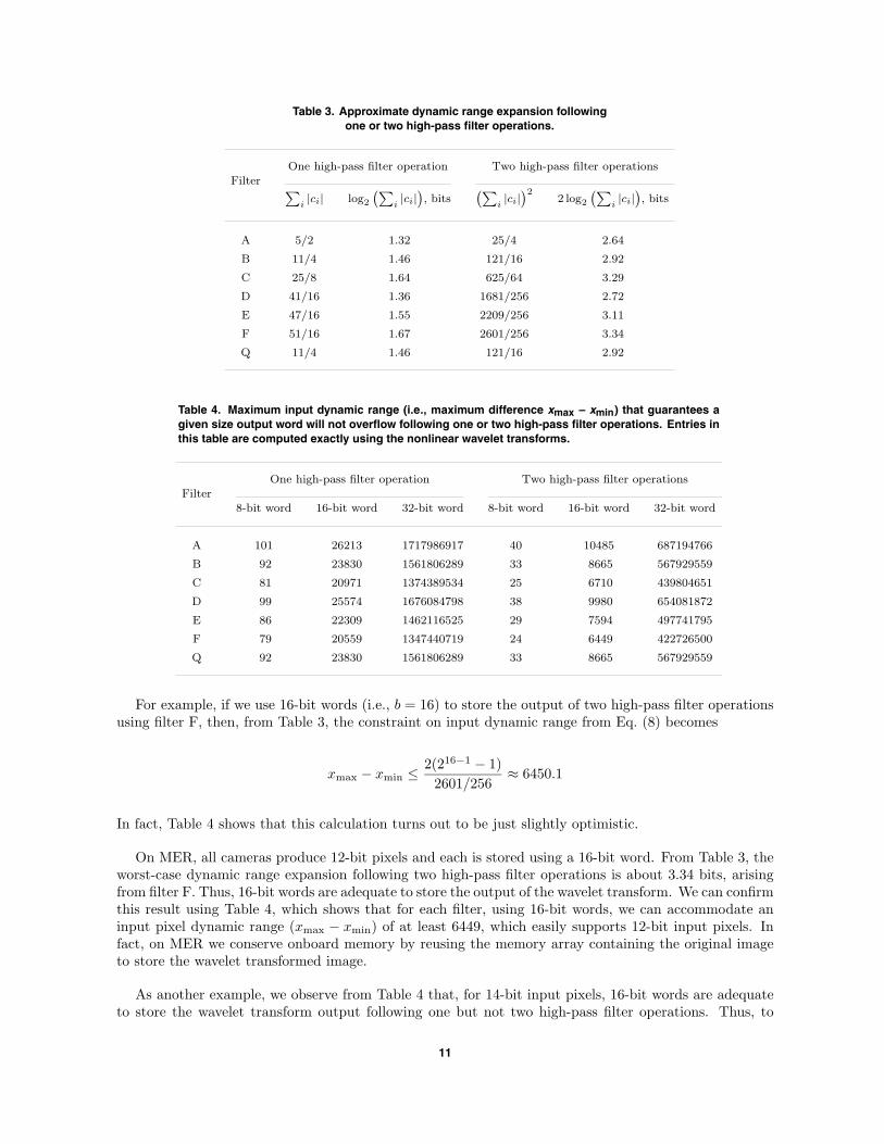
Table 3. Approximate dynamic range expansion followingone or two high-pass filter operations.

One high-pass filter operation Two high-pass filter operationsFilter ∑

i|ci| log2

(∑i|ci|

), bits

(∑i|ci|

)22 log2

(∑i|ci|

), bits

A 5/2 1.32 25/4 2.64

B 11/4 1.46 121/16 2.92

C 25/8 1.64 625/64 3.29

D 41/16 1.36 1681/256 2.72

E 47/16 1.55 2209/256 3.11

F 51/16 1.67 2601/256 3.34

Q 11/4 1.46 121/16 2.92

Table 4. Maximum input dynamic range (i.e., maximum difference xmax – xmin) that guarantees agiven size output word will not overflow following one or two high-pass filter operations. Entries inthis table are computed exactly using the nonlinear wavelet transforms.

One high-pass filter operation Two high-pass filter operationsFilter

8-bit word 16-bit word 32-bit word 8-bit word 16-bit word 32-bit word

A 101 26213 1717986917 40 10485 687194766

B 92 23830 1561806289 33 8665 567929559

C 81 20971 1374389534 25 6710 439804651

D 99 25574 1676084798 38 9980 654081872

E 86 22309 1462116525 29 7594 497741795

F 79 20559 1347440719 24 6449 422726500

Q 92 23830 1561806289 33 8665 567929559

For example, if we use 16-bit words (i.e., b = 16) to store the output of two high-pass filter operationsusing filter F, then, from Table 3, the constraint on input dynamic range from Eq. (8) becomes

xmax − xmin ≤ 2(216−1 − 1)2601/256

≈ 6450.1

In fact, Table 4 shows that this calculation turns out to be just slightly optimistic.

On MER, all cameras produce 12-bit pixels and each is stored using a 16-bit word. From Table 3, theworst-case dynamic range expansion following two high-pass filter operations is about 3.34 bits, arisingfrom filter F. Thus, 16-bit words are adequate to store the output of the wavelet transform. We can confirmthis result using Table 4, which shows that for each filter, using 16-bit words, we can accommodate aninput pixel dynamic range (xmax − xmin) of at least 6449, which easily supports 12-bit input pixels. Infact, on MER we conserve onboard memory by reusing the memory array containing the original imageto store the wavelet transformed image.

As another example, we observe from Table 4 that, for 14-bit input pixels, 16-bit words are adequateto store the wavelet transform output following one but not two high-pass filter operations. Thus, to

11

conserve memory, in principle one could use 32-bit words to store the subbands resulting from two high-pass filter operations (this represents less than a third of the transformed pixels) and 16-bit words for theother subbands.

While the output dynamic range from the high-pass filter is expanded compared to the input dynamicrange, it is observed that the actual range of output values following high-pass filtering tends to besmaller than the range of original pixel values when applied to natural images. Thus, even when overflowis possible, it may be rare. As a test, we produced a “pure noise” image with pixel values independentlydrawn from a uniform random distribution over [0, 214−1]. Following high-pass filtering in the horizontaland vertical directions using filter B, we observed overflow of 16-bit words on only about 0.07 percent ofthe pixels in the resulting HH subband.

D. Quantitative Filter Comparison

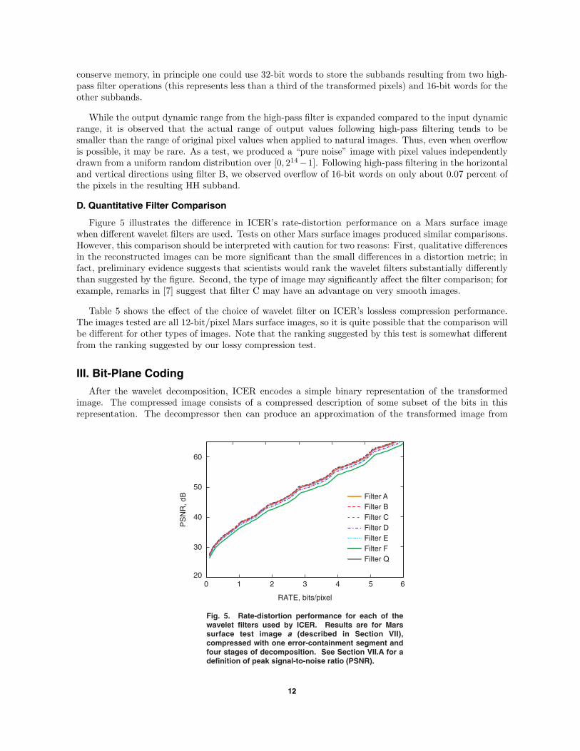
Figure 5 illustrates the difference in ICER’s rate-distortion performance on a Mars surface imagewhen different wavelet filters are used. Tests on other Mars surface images produced similar comparisons.However, this comparison should be interpreted with caution for two reasons: First, qualitative differencesin the reconstructed images can be more significant than the small differences in a distortion metric; infact, preliminary evidence suggests that scientists would rank the wavelet filters substantially differentlythan suggested by the figure. Second, the type of image may significantly affect the filter comparison; forexample, remarks in [7] suggest that filter C may have an advantage on very smooth images.

Table 5 shows the effect of the choice of wavelet filter on ICER’s lossless compression performance.The images tested are all 12-bit/pixel Mars surface images, so it is quite possible that the comparison willbe different for other types of images. Note that the ranking suggested by this test is somewhat differentfrom the ranking suggested by our lossy compression test.

III. Bit-Plane Coding

After the wavelet decomposition, ICER encodes a simple binary representation of the transformedimage. The compressed image consists of a compressed description of some subset of the bits in thisrepresentation. The decompressor then can produce an approximation of the transformed image from

Filter A

Filter QFilter FFilter EFilter DFilter CFilter B

RATE, bits/pixel

PS

NR

, dB

0 1 2 3 4 5 620

30

40

50

60

Fig. 5. Rate-distortion performance for each of the wavelet filters used by ICER. Results are for Mars surface test image a (described in Section VII), compressed with one error-containment segment and four stages of decomposition. See Section VII.A for a definition of peak signal-to-noise ratio (PSNR).

12

Table 5. Lossless compression performance (rate in bits/pixel) for each of thewavelet filters used by ICER. Results are given for the 6 Mars surface test imagesdescribed in Section VII. Images a through e were compressed using 4 stagesof decomposition, and the larger image m was compressed using 6 stages ofdecomposition. A single error-containment segment was used in each case.

FilterImage

A B C D E F Q

a 8.25 8.19 8.20 8.20 8.22 8.26 8.24

b 8.97 8.90 8.90 8.92 8.92 8.96 8.96

c 9.16 9.08 9.08 9.11 9.11 9.15 9.15

d 9.48 9.40 9.40 9.42 9.42 9.46 9.46

e 8.83 8.76 8.76 8.78 8.78 8.82 8.82

m 8.47 8.36 8.32 8.41 8.37 8.38 8.46

Average 8.86 8.78 8.78 8.81 8.80 8.84 8.85

these bits and use the inverse wavelet transform to reconstruct an approximation of the original image.Other specific forms of this general compression strategy can be found in [8,11–14]. In this section, wediscuss two key aspects of the strategy: the order in which the bits are encoded and the estimation ofprobabilities-of-zero of the bits.

Following the wavelet transform, the image subbands are partitioned into segments for error-contain-ment purposes, as described in Section V. The mean value of each segment of the LL subband is computedand subtracted from each pixel in the subband segment. (These mean values are stored in the headersof the corresponding segments so that the original values can be reconstructed.) After this step, theLL subband will in general contain both positive and negative values, even if the original pixel valueswere all positive.

ICER next converts all pixels in the transformed image to sign-magnitude form, i.e., each pixel isstored as a single sign bit along with several magnitude bits.7 Conceptually, a subband can then beregarded as containing several subband bit planes: the most-significant magnitude bits of the pixels in thesubband collectively form a single bit plane, the next most-significant magnitude bits of the pixels formanother bit plane, and so on. Subband bit planes are further divided into error-containment segmentsusing the partitioning of the subbands described in Section V.

ICER losslessly compresses the bit planes of a subband, starting with the most-significant bit plane andworking toward the least significant. Compression of a subband bit plane proceeds one error-containmentsegment at a time, and the bits within a segment are compressed in raster scan order. The sign bits arehandled differently: the sign bit of a pixel is encoded immediately after its first nonzero magnitude bit.

Bit planes from different subbands are interleaved during this coding process. Ideally, after completingcompression of a subband bit plane, ICER would next compress the subband bit plane that gives thebiggest improvement in some measure of image quality per compressed bit. However, there is no easy wayto determine the subband that optimizes such a metric, and the gain in compression effectiveness fromdoing so would be rather modest in any case. Thus, ICER selects the next subband bit plane accordingto a simple prioritization scheme, described in Section III.A.

7 It does not matter what sign bit is given to a pixel with the value 0 because the sign bit of such a pixel is never used.

13

Before encoding a bit, the encoder calculates an estimate of the probability that the bit is a zero.This probability-of-zero estimate relies only on previously encoded information from the same segment.We describe the mechanism for forming this estimate in Section III.A. The bit and its probability-of-zeroestimate are sent to the entropy coder, which compresses the sequence of bits it receives (see Section IV).

The decompressor decodes bits within an error-containment segment in the same order they wereencoded. Before decoding a bit, the decompressor therefore has available all of the information used bythe encoder to produce the bit’s probability-of-zero estimate, and thus can calculate the same estimate,which is essential for proper decoding. This scheme requires a bit-wise adaptable entropy coder, i.e., onewith the ability to update probability estimates with each new coded bit; ICER’s entropy coder, describedin Section IV, has this capability.

ICER employs a technique known as context modeling in computing probability estimates. With thistechnique, a bit to be encoded first is classified into one of several contexts based on the values of previouslyencoded bits. The intent is to define contexts so that bits in the same context will have about the sameprobability-of-zero, and the compressor will be able to estimate this probability reasonably well from thebits it encounters in the context. We describe the specific context definitions in Section III.B and thecalculation of probability estimates in Section III.C.

A well-designed context modeling scheme makes use of as much relevant contextual information aspossible without producing too many contexts. Ignoring relevant contextual information (for example,by defining too few contexts) means that relevant dependencies are not exploited and results in lessinformative probability estimates, hurting compression effectiveness. On the other hand, if too manycontexts occur, then the encoder will not be able to produce good probability estimates because it willnot observe enough bits in many of the contexts.

ICER’s scheme for classifying a bit of a pixel into a context is based on the previously encodedbits in pixels in the immediate neighborhood of the pixel. Some earlier methods [8,11] for compressingsubband bit planes exploited similarities between different subbands, with reasonable success. However,more recent studies suggest that context models exploiting information from the immediate nine-pixelneighborhood within the given subband will gain very little from also exploiting correlations with differentsubbands (or, for that matter, pixels in the subband but outside this neighborhood) [13,15]. Furthermore,basing the context only on pixels in the immediate subband simplifies encoding. The particular contextscheme used by ICER is derived from the scheme used by the Embedded Block Coding with OptimizedTruncation (EBCOT) compressor [13] and JPEG 2000 [14], and is described in detail in Section III.B.

A. Subband Quantization and Priority Factors

Reconstructing a subband from one or more of its most-significant bit planes and the sign bits of pixelsthat are nonzero in at least one of these bit planes is equivalent to applying a certain scalar quantizer toeach pixel of the original subband. This quantizer has quantization bins with uniform width ∆ exceptfor a central “deadzone” bin with width 2∆− 1, where ∆ = 2b and b is the number of bit planes that areunavailable. Figure 6 illustrates an example of this quantizer. Including further bit planes (decreasing b)amounts to successively refining the quantizer, halving ∆ for each additional bit plane.

D 2D - 1

Fig. 6. Effective “deadzone” quantizer after three magnitude bits have been transmitted.

14

Since the wavelet transforms used by ICER produce integer outputs, we can identify ranges of integerscorresponding to the quantization bins. The center deadzone bin, which corresponds to the interval[−(∆− 1),∆− 1], is symmetric about the origin and, thus, we use the origin as its reconstruction point.Every other bin corresponds to an interval of the form ±[i∆, (i + 1)∆ − 1], where i is a positive integer.If ∆ = 1, then all bit planes are available, and the pixels in the subband are reconstructed exactly.Otherwise, we use the integer ±((i + 1/2)∆ − 1) as the reconstruction point for the bin. This point isslightly biased towards the origin since the distribution of the wavelet-transformed pixel values tends tobe peaked at the origin for all but the LL subband (and the interval contains ∆ = 2b points, an evennumber, so the midpoint is not an integer anyway).

Subband pixel values in all but the LL subband tend to have sharply peaked and roughly symmetricdistributions. For such a distribution, the deadzone quantizer induced by the bit-plane compressionscheme gives better rate-distortion performance than a uniform quantizer when used for progressivecompression. This is demonstrated in [16] for a Laplacian source.

Quantization of the subband data introduces distortion into the reconstructed image. Since the filtersused by ICER are not unitary (in fact the linear filters that they approximate are not even orthogonal),the mean-square-error (MSE) distortion computed in the transform domain is not equal to the MSE ofthe reconstructed image. However, the scaled version of the transform given by �[n] =

√2�[n], h[n] =

(1/√

2)h[n] is approximately unitary and, thus, the weights shown in Fig. 7 can be used to determinethe relative priorities of subband bit planes [7]. These weights indicate the approximate relative effect(per pixel of the subband) on the reconstructed image of root-mean-squared (RMS) distortion values inthe subbands. Combining this weighting with the fact that each additional bit plane reduces the RMSdistortion in a subband by roughly a factor of 2 yields relative priority weights for all subband bit planes.

For example, after three stages of wavelet decomposition, a pixel in the LL subband has a factor of 16higher priority weight than a pixel in the level-1 HH subband. Thus, in this case the ith least-significantbit plane of the level-1 HH subband has priority equal to that of the (i + 4)th least-significant bit planeof the LL subband.

ICER uses this priority scheme to determine the order in which to encode subband bit planes. Whenmultiple subband bit planes have the same priority, ICER gives precedence to those in the subbands witha higher decomposition level. When the decomposition level is also the same, the precedence depends onthe type of subband, in this order: LL, HL, LH, HH.

1

1

1

2

22

4

48

1/2

Fig. 7. Priority weights of sub-bands, shown for three stages of wavelet decomposition.

15

B. Context Assignment

In ICER, the context of a bit in a pixel is determined by the bits already encoded in the pixel and inits eight nearest neighbors from the same segment of the subband. Thus, from the more-significant bitplanes, bits from all nine of these pixels help to determine the context; from the current bit plane, bitsfrom only four of these pixels are used (they are determined by the raster-scan encoding order withinbit-plane segments). See Fig. 8.

As it compresses bit planes, ICER keeps track of a category for each pixel. A pixel’s category summa-rizes information about the bits already encoded in the pixel, facilitating the capture of relevant contextualinformation with a small number of contexts. ICER uses four pixel categories that are based on the con-cept of significance of a pixel [11]: a pixel is not significant if the magnitude bits already encoded in thepixel are all zeros; otherwise, the pixel is significant. We label the categories as 0, 1, 2, and 3. A pixel’scategory is 0 if it is not yet significant; after the first ‘1’ bit from the pixel is encoded, the pixel’s categorybecomes 1; when the next magnitude bit from the pixel is encoded, the pixel’s category becomes 2; and,finally, when one more magnitude bit from the pixel is encoded, the pixel’s category becomes 3 and re-mains 3 permanently. Figure 9 provides an example of the categories a pixel goes through as it is encoded(here MSB and LSB denote the most-significant bit and least-significant bit, respectively).

Bits to be encoded that are likely to be compressible are classified into one of 17 contexts; as mentionedabove, this classification scheme is derived from that of EBCOT [13] and JPEG 2000 [14]. Contexts 0through 8 are used for bits of pixels that are not yet significant (that is, pixels in category 0). Contexts 9and 10 are used for bits of pixels that have just become significant (pixels in category 1). Context 11 isused for bits of pixels in category 2. Contexts 12 through 16 are used for sign bits.

Bits of pixels in category 3 are empirically nearly incompressible; that is, estimates of these bits’probabilities-of-zero tend to be very close to 1/2. Therefore, these bits are left uncoded in the compressor’soutput.8

The context of a bit is determined using the category of the pixel containing the bit and the significanceand signs of the 8 adjacent pixels. If not all of the 8 adjacent pixels are available because the pixel beingencoded is at the edge of its subband segment, the missing pixels are treated as being not yet significant.

a

a x b

bbb

a a

Fig. 8. When encoding a bit of the pixel “x,” the context is determined by bits already encoded in the nine pixels shown. Magnitude bits from the current and more significant bit planes are available from the “a” pixels, while only magnitude bits from the more significant bit planes are available from pixel “x” and the “b” pixels.

8 More precisely, they are sent directly to the “uncoded” bin of the interleaved entropy coder (see Section IV), implicitlyassuming a probability-of-zero of 1/2.

16

0 01 1 0 1 0 1

0 0

0

Category

0 0 0

0 01 1 1

0 01 1 0 2

0 01 1 0 1 3

0 01 1 0 1 0 3

3

SignBit Magnitude Bits

MSB LSB

Enc

odin

g P

rogr

essi

on

Fig. 9. Example of the progression of categories of a pixel as its magnitude bits and sign are encoded. The pixel shown has value –21, and an 8-bit representation is assumed (7 magnitude bits preceded by a sign bit). Bits not yet encoded are shaded. Between each state shown, a magnitude bit is encoded as part of the encoding of a subband bit plane. This pixel’s sign bit is encoded with the third most-significant bit plane.

We first describe the contexts for bits of pixels in category 0. If the subband being encoded is not anHL subband, then let h be the number of horizontally adjacent pixels that are significant (0, 1, or 2), v bethe number of vertically adjacent pixels that are significant (0, 1, or 2), and d be the number of diagonallyadjacent pixels that are significant (0–4). For an HL subband, the roles of h and v are reversed, effectivelytransposing the context template. Given h, v, and d, the context is assigned according to Table 6 if thesubband is not an HH subband; otherwise, the context is assigned according to Table 7.

A bit of a pixel in category 1 is assigned context 9 if none of the horizontally or vertically adjacent pixelsis significant; otherwise, it is assigned context 10. A bit of a pixel in category 2 is assigned context 11regardless of the categories of adjacent pixels.

Sign bits are not encoded directly; rather, the context modeler first predicts the sign bit and then en-codes an “agreement” bit that is the exclusive-or of the sign bit and its predicted value. The agreement-bitstatistics associated with a sign context are used to estimate a probability-of-zero for future agreementbits in the context in exactly the same manner as magnitude bits in magnitude contexts. The prediction of

Table 6. Contexts for bits of pixels in category 0 in LL, LH, and HLsubbands, as a function of h, v, and d.

h = 0 h = 1d h = 2

v = 0 v = 1 v = 2 v = 0 v > 0

d = 0 0 3 4 5 7 8

d = 1 1 3 4 6 7 8

d ≥ 2 2 3 4 7 7 8

17

Table 7. Contexts for bits of pixels in category 0 in HHsubbands, as a function of h + v and d.

d h + v = 0 h + v = 1 h + v ≥ 2

d = 0 0 1 2

d = 1 3 4 5

d = 2 6 7 7

d ≥ 3 8 8 8

sign bits allows the number of contexts to be reduced, as suggested by the following reasoning: Suppose Aand B are pixels with as-yet-unencoded signs. If the pixels in the neighborhood of A are the negatives ofthe corresponding pixels in the neighborhood of B, then by symmetry we should expect the probabilitythat A is positive is about the same as the probability that B is negative. Therefore, the agreement bitsfor both pixels’ signs can be sensibly encoded with the same context, even if the sign bits themselvescould not be.

ICER uses the two horizontally adjacent and the two vertically adjacent pixels to determine both thesign estimate and the context. If the subband is not an HL subband, let h1 and h2 represent the signsand significances of the two horizontally adjacent pixels, taking on the values 1, −1, and 0 for pixels thatare positive, negative, and not significant, respectively. Similarly, let v1 and v2 represent the signs andsignificances of the two vertically adjacent pixels. For the HL subband, the roles of the h’s and v’s areagain reversed. Otherwise, the different types of subbands are treated the same with respect to encodingsign bits. Table 8 lists the sign estimate and the context as a function of h1 + h2 and v1 + v2.

C. Probability Estimation

For each context, ICER maintains nominal counts of the number of zero bits and the total number ofbits that have occurred in the context; the ratio of these counts represents the probability-of-zero estimatefor the context. For each bit to be encoded, the entropy coder receives the probability-of-zero estimatein the form of the ratio of these counts.

Each context’s counts are initialized to values corresponding to a probability-of-zero of 1/2. Eachbit encountered in a context increments the total count, and increments the count of zeros if the bitis a 0. (Of course, these increments occur after the bit is encoded.) When the total count reaches aspecified value, both counts are rescaled by dividing by 2 (when necessary, the count of zeros is roundedin the direction that makes the probability-of-zero estimate closer to 1/2). The rescaling has the effectof producing probability-of-zero estimates that give more weight to recent bits, accommodating to somedegree context statistics that change as the compression proceeds.

In our MER implementation, the initial counts of zeros are set to 2, the initial total counts are setto 4, and rescaling is triggered when the total count reaches 500.

Table 8. Sign bit predictions and sign contexts.

v1 + v2 h1 + h2 < 0 h1 + h2 = 0 h1 + h2 > 0

v1 + v2 < 0 −, 16 +, 13 +, 14

v1 + v2 = 0 −, 15 +, 12 +, 15

v1 + v2 > 0 −, 14 −, 13 +, 16

18

D. Coding Differences between ICER, EBCOT, and JPEG 2000

ICER’s bit-plane coding has many similarities to bit-plane coding in EBCOT [13] and JPEG 2000[14]. Most notably, the context scheme used by ICER is derived from that of EBCOT (whose contextscheme is nearly the same as that of JPEG 2000). However, there are also many differences in how thethree compressors perform bit-plane coding. We mention some of the bigger differences here. We alsopoint out differences related to entropy coding.

EBCOT and JPEG 2000 organize subbands into smaller units in a way that is somewhat different fromICER’s organization of subbands into error-containment segments. JPEG 2000 uses a more complicatedorder for encoding subband bit planes than the simple raster-scan order used in ICER. During encoding,EBCOT transposes HL subbands, while ICER and JPEG 2000 transpose only the context template ofsuch subbands (see Section III.B). ICER makes just one pass through each subband bit plane; JPEG 2000makes three passes, each pass encoding a different subsets of bits; and EBCOT makes four such passes,one of which is in reverse raster-scan order.

There are several differences in the way the three compressors perform probability estimation andentropy coding. JPEG 2000 uses an approximate arithmetic coder (the MQ coder from the JBIG2standard [17]) for entropy coding; EBCOT uses more standard arithmetic coding; and ICER uses aninterleaved entropy coder (see Section IV). Probability estimation in JPEG 2000 is performed usinga state table incorporated in the arithmetic coding process. EBCOT and JPEG 2000 group 4 bitstogether (in a form of run-length coding) prior to entropy coding under certain circumstances; ICERdoes not do anything similar to this. ICER regards certain bits as incompressible and leaves themuncoded (see Section III.B); this is similar to the “lazy coding” option in JPEG 2000, but EBCOT hasnothing analogous. Finally, JPEG 2000 uses skewed initial statistics for some contexts so that the initialprobability-of-zero estimates for bits in these contexts are not 1/2; this can slightly improve compressioneffectiveness on typical images. EBCOT and ICER use unskewed initial statistics for all contexts (seeSection III.C).

IV. Entropy Coding

In this section, we describe the entropy coder used by ICER to compress the magnitude and sign bitsof the pixels in the wavelet-transformed image.

A. Adaptable Entropy Coding

In a sequence of source bits b1, b2, · · · from the subbands, for each bit bi the context modeler describedin Section III produces an estimate pi of the probability that bi equals zero. The entropy coder usesthese estimates to produce an encoded (and hopefully compressed) bitstream from which the original bitsequence can be reconstructed.

ICER uses a bit-wise adaptable entropy coder. Thus, the probability estimate pi can depend on thevalues of previous bits and change with each new bit, allowing the context modeler to quickly adapt tochanging statistics and make better use of the immediate context in which a bit appears. Accommodatinga probability estimate that varies from bit to bit in this way is tricky because the decompressor needs toconstruct the same estimates as the compressor. Thus, the decompressor must determine the values ofthe first i − 1 bits before it can decode the ith bit.

Although adaptable binary entropy coding usually is performed using arithmetic coding [18] (or witha low-complexity approximation to arithmetic coding such as that described in [19]), we have chosen touse a lesser-known technique called interleaved entropy coding [20–22]. Given perfect probability esti-mates, practical implementations of both arithmetic coding and interleaved entropy coding can compressstochastic bit sequences to within 1 percent of the theoretical limit, but interleaved entropy coding hassome speed advantages [21].

19

Interleaved entropy coding was first suggested in [23] and has also appeared in [20,24]. In [21], weintroduce recursive interleaved entropy coding, a generalization of the technique. References [21,22]contain a thorough description of recursive and non-recursive interleaved entropy coding. In the trade-off between encoding speed and compression effectiveness, non-recursive coders generally outperformrecursive coders. Thus, we have used a non-recursive coder in ICER, and in the remainder of this articlethe discussion of interleaved entropy coding will implicitly refer to the non-recursive type. Our softwareimplementation of the coder in ICER has particularly low complexity, and so is well-suited for spaceapplications and other applications where encoding speed can be of critical importance.

In the remainder of this section, we give a brief overview of interleaved entropy coding and specify theparticular coder design used in ICER.

B. Variable-to-Variable-Length Codes

An interleaved entropy coder combines several component source codes. Each component code is avariable-to-variable-length binary source code, which is a mapping from a set of input codewords to a setof output codewords. Variable-to-variable length means that in general neither the input codewords northe output codewords all have the same length. An encoder for such a code parses a sequence of inputbits into input codewords. The encoder output consists of the concatenation of the corresponding outputcodewords. Decoding is accomplished using the same procedure as encoding, with the roles of input andoutput codeword sets reversed.

An example of a variable-to-variable-length binary source code is given in Table 9 (this code is theGolomb code [25] with parameter m = 5; see below for a description of the family of Golomb codes).With this code, the binary sequence 0100000001100001 is parsed as 01, 00000, 001, 1, 00001, resulting inthe encoded output sequence 001, 1, 010, 000, 0111.

For every component code, the input and output codeword sets are each prefix-free, which means thatno codeword is a prefix of another codeword in the set, and exhaustive, which means that no codeword canbe added to the set without violating the prefix-free condition. These properties ensure that a sequenceof bits can be uniquely parsed into codewords and that we recognize a complete codeword as soon as itis formed, i.e., without looking ahead in the sequence.

Several of the component codes in ICER’s entropy coder are Golomb codes [25,26], which are ef-ficient for encoding long runs of bits having nearly the same probability-of-zero, especially when thatprobability-of-zero is near 1. We denote particular Golomb codes with the notation Gm, where m ≥ 1.The code Gm has m + 1 input codewords: 1, 01, 001, · · · , 0m−11, and 0m. (We use the notation 0i todenote a run of i zeros.) Input codeword 0m maps to the output codeword consisting of a single 1. To de-scribe the output codewords for the other input codewords, we let � = �log2 m� and i = 2�−m. The output

Table 9. The Golomb code withparameter m = 5.

Input codeword Output codeword

00000 1

00001 0111

0001 0110

001 010

01 001

1 000

20

codeword corresponding to input codeword 0k1 is the �-bit binary representation of integer k when k < i,and the (� + 1)-bit representation of the integer k + i otherwise.

C. Interleaved Entropy Coding

An interleaved entropy coder compresses a binary source with a bit-wise adaptive probability estimateby interleaving the output of several different variable-to-variable-length binary source codes that eachencode groups of bits with similar probability estimates. Much variation is possible in the choice andnumber of component codes, yielding coder designs of varying complexity and compression efficiency.

Without loss of generality, we may assume that pi ≥ 1/2 for each index i. If this is not the case forsome pi, we simply invert bit bi before encoding to make it so; this inversion clearly can be duplicatedin the decoder. Thus, we are concerned with the probability region [1/2, 1]. We partition this regioninto several narrow intervals or bins, and for each bin we define a component code designed to effectivelycompress sequences of bits having probabilities-of-zero lying in this interval. Bit bi is encoded (along withother source bits) using the source code corresponding to the interval containing pi.

For example, one of the bins of ICER’s entropy coder corresponds to a probability interval approxi-mately equal to (0.85, 0.88) and uses the Golomb code G5 shown in Table 9. To give an indication of howwell this code performs in this interval, we can evaluate the compression effectiveness of this code whenapplied to an independent and identically distributed (IID) binary source that produces zeros with fixedprobability p in this interval. A short calculation shows that the average input codeword length equals1 + p + p2 + p3 + p4 and the average number of output bits per codeword is 3 + p3 − 3p5 for this source.Thus, the average rate is

r(p) =3 + p3 − 3p5

1 + p + p2 + p3 + p4(bits/source bit)

and the redundancy is r(p) −H2(p) where

H2(p) = −p log2 p − (1 − p) log2(1 − p)

is the binary entropy function, the theoretical limit of compression achievable for this source. Figure 10shows that the redundancy for this example is small when p is in the appropriate range.

The output of any interleaved entropy coder contains some redundancy because, for example, sourcebits with slightly different estimated probabilities-of-zero are treated the same; that is, the bins’ intervalshave positive widths. However, by using an increasing number of increasingly large variable-to-variable-length codes, one can produce a coder design with redundancy as small as desired (asymptotically as theinput sequence length becomes long), given a stochastic source with perfect probability estimates [21].

We now give brief descriptions of the encoding and decoding procedures. Refer to [21,22] for a morecomplete treatment.

1. Encoding. The encoder groups bits from the same bin together to form input codewords. Toensure that decoding is possible, the output codewords produced by the different component codes must beinterleaved in the proper order. The encoder accomplishes this by maintaining a list of input codewordsand partially formed input codewords in a circular buffer. In the MER implementation of ICER, thecircular buffer has a capacity of 2048 words.

When source bit bi arrives, it is assigned to the bin whose probability interval contains the bit’sprobability-of-zero estimate pi. The encoder then checks whether the list includes a partial input codeword

21

PROBABILITY-OF-ZERO

0.86 0.87 0.88

RE

DU

ND

AN

CY,

bits

/sou

rce

bit

0.000

0.001

0.002

0.003

0.004

0.005

0.006

Fig. 10. Redundancy for the Golomb code G5 used on an IID binary source with fixed probability-of-zero. ICER uses this code for the probability-of-zero range covered by this graph.

for this bin. If so, the bit is appended to this partial codeword. Otherwise, the bit begins a new word atthe end of the list.

When the word at the beginning of the list is a complete input codeword for the correspondingcomponent code, the encoder produces the corresponding output bits and the word is removed from thelist, making more room available for new words. If the new beginning position of the list contains acomplete codeword, it also is processed in this manner, and so on.

If the buffer containing the word list becomes full, one or more “flush bits” are appended to the(necessarily partial) input codeword at the front of the list to form a complete codeword that is thenprocessed in the normal manner. Flushing of a partial input codeword is accomplished by producing theshortest output codeword that is consistent with the bits already in the partial codeword; in practice,the appropriate output codewords corresponding to partial input codewords are tabulated in advance.Flush bits also are used to complete all partial codewords remaining in the list of words once the inputbit sequence is exhausted.

2. Decoding. The decoder is somewhat simpler than the encoder. The decoder keeps track of apartial input codeword for each bin of the coder. In the decoder, each such word is a suffix of an inputcodeword for the bin. Codewords are reconstructed in the decoder in the same order that they appearedin the encoder’s list.

Source bits are decoded in order. To decode bi, the decoder calculates the associated probabilityestimate pi, which in general may be based on the values of preceding source bits just decoded. Given pi,the decoder uses the same procedure as the encoder to determine the bin to which bit bi was assignedby the encoder. If the decoder has a partial codeword for this bin, the first remaining bit of this partialcodeword is removed; this bit becomes the decoded bit bi. Otherwise, the decoder must reconstruct aninput codeword of the component code for the bin; this is accomplished by parsing an output codewordfrom the next available bits in the encoded bitstream and determining the corresponding input codeword.The first bit of this codeword becomes the decoded bit, and the decoder remembers the remainingcodeword suffix.

22

For proper decoding, the decoder must identify and remove flush bits so that they are not mistaken forsource bits. Fortunately, this is straightforward. While decoding, the decoder keeps count of the numberof codewords reconstructed. Each time a codeword is reconstructed, the decoder stores this count alongwith the codeword suffix. When the difference between the current count and the value associated with agiven codeword suffix exceeds the size of the encoder’s buffer, then all of the remaining bits in this suffixmust be flush bits and are discarded. Identification of flush bits can be accomplished quite efficiently; in[22] we describe several approaches in detail.

D. ICER’s Interleaved Entropy Coder

In this section, we specify the particular interleaved entropy coder design used by ICER.

We first describe a shorthand notation, similar to that introduced in [21], that we use to specify someof the component codes. As an alternative to a code table, a variable-to-variable-length source code canbe specified by a tree that provides a map for decoding. For example, Fig. 11 shows a decoding tree forthe Golomb code G5 of Table 9. Each input codeword is assigned to a leaf in the tree, and the branchlabels, each a zero or one, indicate the output bits. The output codeword assigned to an input codewordis the sequence of branch labels from the root to the leaf for that input codeword. Thus, to decode, westart at the root, traversing a branch for each encoded bit read, until we reach the input codeword at theleaf. (Similarly, one could construct an encoder-oriented tree.)

We use a shorthand description of the decoding tree as a compact specification of a component code.For each terminal node, we write the corresponding input codeword. A non-terminal node is representedby an ordered pair containing the representations of the child nodes, with the node associated with a zerooutput bit listed first. Thus, using this shorthand, the Golomb code G5 shown in Fig. 11 and Table 9 alsocan be represented as

( ((1, 01),

(001, (031, 041)

)), 05

)

An interleaved entropy coder design is specified by giving the probability interval and the componentsource code used for each bin. The bins are indexed starting from 1, with lower indices assigned toprobability intervals closer to 1/2. The intervals may be specified by probability cutoffs zj so that bin jcorresponds to probability interval [zj−1, zj), where z0 is taken to be 1/2.

Table 10 specifies ICER’s entropy coder design, which has 17 bins. To simplify the comparison betweenprobability estimates and cutoffs, we use cutoffs that are rational numbers with denominator 216. Bits in

11

1

1

0

0

0

01

0001

00001

001

1

0

1

0

00000

Fig. 11. A decoding tree for the Golomb code G5. Output bits are shown in boldface. The input codewords are shown at terminal nodes of the trees.

23

Table 10. The interleaved entropy coder design used by ICER.

Bin ProbabilityCode

index j cutoff zj

1 35298/65536 (0,1) (uncoded)

2 37345/65536 (((((041, 14), 031), 001), 10), (01, (110, (05, 130))))

3 40503/65536 (((001, ((1101, 0311), 13)), 10), (01, (04, (1100, 0310))))

4 43591/65536 ((03, 01), (10, (001, 11)))

5 47480/65536 (((010, (104, 110)), ((101, 011), ((1031, 13), 1001))), 00)

6 50133/65536 ((05, 1), ((031, 001), (010, (041, 011))))

7 53645/65536 (03, ((001, 010), (100, (11, (011, 101)))))

8 55902/65536 (04, ((001, 01), (10, (0310, (0311, 11)))))

9 57755/65536 G5

10 58894/65536 G6

11 60437/65536 G7

12 62267/65536 G11

13 63613/65536 G17

14 64557/65536 G31

15 65134/65536 G70

16 65392/65536 G200

17 65536/65536 G512

the first bin, whose interval contains probability 1/2, are incompressible (or nearly so), and are unchangedby the coding process. For this bin, each source bit forms a complete input codeword, and each outputcodeword equals the input codeword. The component codes for bins 2 through 8 are specified usingour shorthand notation for the code’s tree. For bins 9 through 17, corresponding to probability-of-zeroestimates larger than 55902/65536 ≈ 0.853, ICER uses the Golomb codes indicated in the table.

As an indication of the effectiveness of ICER’s entropy coder, Fig. 12 shows the asymptotic redundancyobtained when the coder is used to compress an IID source with fixed but known probability-of-zero. Thegraph shows that, for a stochastic source with perfect probability estimates, the redundancy contributionfrom ICER’s entropy coder is quite small. Thus, to improve ICER’s compression effectiveness, we wouldbe more inclined to invest our efforts in an area such as improved context modeling rather than tryingto reduce the redundancy of ICER’s entropy coder.

V. Error Containment

Data-compression methods are more effective when they exploit dependencies between the data beingcompressed and previously compressed data in the same image or data set. However, a drawback ofexploiting such dependencies, especially over large data sets, is that if a portion of compressed data islost, then decoding of subsequent dependent portions is impossible.

Thus, to mitigate the impact of data losses that occur on the deep-space communications channel, adata compressor must incorporate effective error-containment techniques. Without error containment,even a small loss of data can render useless large portions of compressed data. Error containment can beachieved by dividing the data set into segments that are compressed independently, so that when datafrom one segment are lost or corrupted, reconstruction of the other segments is unaffected.

In this section, we describe data-loss mechanisms of the deep-space channel and ICER’s particularerror-containment strategy.

24

PROBABILITY-OF-ZERO

RE

DU

ND

AN

CY,

bits

/sou

rce

bit

0.5 0.6 0.7 0.8 0.9 1.0

0.000

0.001

0.002

0.003

0.004

0.005

0.006

Fig. 12. Redundancy as a function of probability-of-zero when ICER’s interleaved entropy coder is used to compress an IID binary source with a known fixed probability-of-zero. The dashed vertical lines mark the boundaries between bins.

A. Data Loss on the Deep-Space Channel

The Consultative Committee for Space Data Systems (CCSDS) packet telemetry standard [27] definesthe protocol used for the transmission of spacecraft instrument data over the deep-space channel. Underthis standard, an image or other data set from a spacecraft instrument is transmitted using one or morepackets. A packet is a block of data with length that can vary between successive packets, ranging from 7to 65,542 bytes, including the packet header. Packetized data are transmitted via frames, which arefixed-length data blocks. The size of a frame, including frame header and control information, can rangeup to 2048 bytes, but it is fixed during a given mission phase. Because packet lengths are variable butframe lengths are fixed, packet boundaries usually do not coincide with frame boundaries, as illustratedin Fig. 13.

Data in a frame typically are protected from channel errors by error-correcting codes. Even whenthe channel errors exceed the correction capability of the error-correcting code, the presence of errorsnearly always is detected by the error-correcting code or by a separate error-detecting code. Frames forwhich uncorrectable errors are detected are marked as undecodable and typically are deleted. Deletedundecodable whole frames are the principal type of data loss that affects compressed data sets.

There generally would be little to gain from attempting to use compressed data from a frame markedas undecodable. When errors are present in a frame, the bits of the subband pixels already decodedbefore the first bit error will remain intact, but all subsequent decoded bits in the segment usually will

Frame Frame Frame Frame

Packet Packet Packet

Fig. 13. Packet boundaries usually are not aligned with frame boundaries.

25

be completely corrupted; a single bit error is often just as disruptive as many bit errors. Furthermore,compressed data usually are protected by powerful, long-blocklength error-correcting codes, which arethe types of codes most likely to yield substantial fractions of bit errors throughout those frames thatare undecodable. Thus, frames with detected errors would be essentially unusable even if they were notdeleted by the frame processor.

If an erroneous frame escapes detection, the decompressor will blindly use the frame data as if theywere reliable, whereas in the case of detected erroneous frames, the decompressor can base its recon-struction on incomplete, but not misleading, data. Fortunately, it is extremely rare for an erroneousframe to go undetected. For frames coded by the CCSDS Reed–Solomon code [28], fewer than 1 in 40,000erroneous frames can escape detection [29]. All frames not employing the Reed–Solomon code use a cyclicredundancy check (CRC) error-detecting code, which has an undetected frame-error rate of less than 1in 32,000 [30].

To summarize, coding and framing considerations lead us to model the relevant data losses as lossesof whole frames. A frame loss results in the loss of one or more entire or partial packets, depending onthe packet lengths and the alignment between packet and frame boundaries (refer to Fig. 13). When aframe loss eliminates only a portion of a packet, intact data in the packet preceding the loss could beused by the decompressor to reconstruct source data. However, keeping track of partial packets increasesthe complexity of ground operations, and the usual practice is to discard incomplete packets. Thus, theeffective consequence of a frame loss is generally the loss of one or more entire packets.

Since the loss of a single frame may affect more than one packet, for error-containment effectiveness itis important that ICER’s compressed output be arranged so that packets containing data from the samesegment are contiguous, as described in Section VI.B. This arrangement reduces the chance that a singleframe loss affects more than one segment.

B. Error Containment in ICER

To achieve error containment, ICER automatically partitions the image data into a user-specifiednumber of segments. Each segment is compressed independently of the others so that the loss of datafrom one segment does not affect the ability to reconstruct another segment.

To ensure that the segments can be decompressed independently of each other, each compressedsegment begins with a header containing information such as the segment index, image dimensions, andICER parameters. Because each segment is compressed independently, ICER maintains separate contextmodeler and entropy coder data for each segment. When organizing compressed data into packets fortransmission, multiple packets may be used for a single compressed segment, but no packet should containdata from more than one segment.

Conceptually, segmentation occurs after the wavelet decomposition. Each pixel of the transformedimage is assigned to a segment. Although segments are defined in the transform domain, each approx-imately corresponds to a rectangular region of the original image. If s segments are desired, first theLL subband is partitioned into s rectangular segments, and then this partition is mapped to the othersubbands. Thus, pixels in different subbands corresponding to the same spatial location will belong tothe same segment. As a simple example, we illustrate in Fig. 14 the regions of a transformed image cor-responding to a partition into two segments. The remaining problem of how to partition the LL subbandinto rectangles is addressed in Section V.D.

A consequence of defining segments in the wavelet transform domain is that segment boundaries arenot sharply defined in the image domain. To reconstruct pixels near the boundaries between segments,the inverse wavelet transform combines data from adjacent segments. Consequently, the effect of dataloss in one segment can appear to “bleed” slightly into adjacent segments in the reconstructed image; i.e.,a few pixels near the borders of that segment may appear blurred.

26

Fig. 14. A partition of a wavelet-transformed image into two segments, shown here for three stages of wavelet decomposition. The shaded pixels all belong to the left segment.

Defining image segments in the wavelet transform domain has some advantages over the simpleralternative of partitioning the image directly and applying a wavelet decomposition separately to eachsegment (i.e., dividing the original image into smaller images that are compressed independently). Withlossy compression under this simpler alternative, the boundaries between segments would tend to benoticeable in the reconstructed image even when no compressed data are lost, as illustrated in Fig. 15(a).This is, in fact, a larger-scale version of the “blocking” artifact that can occur in JPEG-compressedimages (see Fig. 2(c), for example). By segmenting the image in the transform domain, we can virtuallyguarantee that such artifacts will not occur. Figure 15(b) illustrates the elimination of these artifacts.

By applying the wavelet transform to the entire image at once, we also achieve better decorrelationand reduce inefficiencies associated with the wavelet transform at image boundaries, thus improvingcompression effectiveness.

Because ICER compresses each segment of a subband bit plane before moving on to the next subbandbit plane, each segment will be encoded to nearly the same fidelity. The lengths of compressed segmentswill vary somewhat, in large part because segments that are easier to compress will use fewer bits. Forexample, a segment consisting mostly of smooth sky likely would use fewer bits than a similarly sizedsegment containing highly textured terrain and rocks.

Since each segment is compressed progressively, some error containment automatically occurs withinsegments as well: when a packet loss occurs, any previously received packets for the affected segment willallow a lower-fidelity reconstruction of that segment. Although the decompressor is unable to make useof data in a segment that follows a loss, a packet loss does not eliminate an entire segment unless thepacket lost is the initial packet for the segment. Figure 16 illustrates an image reconstructed followingpacket losses affecting three segments.

(b)(a)

Fig. 15. Image details that illustrate (a) artifacts at segment borders that would arise if the wavelet transform were separately applied to each segment and (b) elimination of such artifacts in the ICER-compressed image.

27

55% Data Loss

100% Data Loss

90% Data Loss

Fig. 16. Example of error containment in an image compressed to 1 bit/pixel, with simulated packet lossesaffecting three of eight image segments.

C. Choosing the Number of Segments

ICER provides flexibility in choosing the number of segments, allowing a user to trade compressioneffectiveness against packet loss protection, thereby accommodating different data loss rates. In general,we would tend to use a larger number of segments for larger images, larger numbers of compressed bytes,and less reliable channels.

Dividing an image into a larger number of segments tends to result in increased protection from dataloss because a loss within a single segment affects a smaller portion of the image. However, there is alimit to the added protection provided by increasing the number of segments: as the segments decrease insize, the number of compressed bytes per segment becomes small, and it becomes more likely that a singleframe loss will affect multiple segments. Moreover, compression effectiveness suffers when image segmentsbecome sufficiently small, in part because smaller segments have less data over which dependencies canbe exploited. Thus, as the number of segments increases, at some point the marginal error-containmentbenefit becomes tiny, and the compression effectiveness cost becomes significant. Note that, for a givennumber of segments, the former is determined primarily by the number of output bytes produced, andthe latter is determined primarily by the image size.

The MER implementation of ICER limits the number of segments to 32 or fewer and imposes tighterlimits when the image is small and the number of stages of wavelet decomposition is large.9 Generally,however, a user has considerable flexibility in choosing the number of segments, especially for large images.

If packet losses are rare or when compressing a small image, one might reasonably set the numberof segments to 1 so that the entire image is treated as a single segment. However, some amount ofsegmentation may slightly improve compression effectiveness, especially on large images. Many images aremost effectively compressed using four to six segments because segmentation can coincidentally separatedisparate regions of the image into different segments (e.g., some segments of an image may consist mostlyof sky and others mostly of soil), allowing the context modeler to develop distinct sets of statistics forthese regions.

9 A. Kiely and M. Klimesh, op. cit.

28

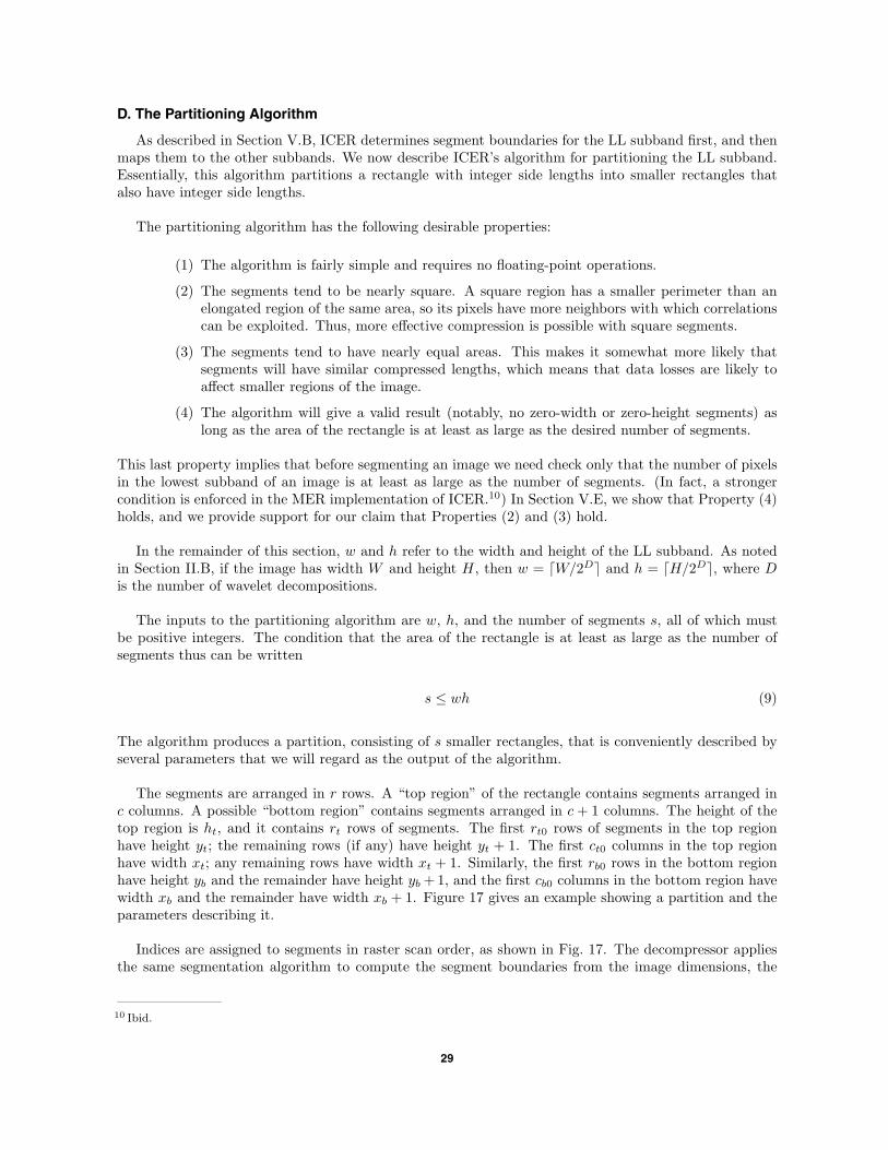
D. The Partitioning Algorithm

As described in Section V.B, ICER determines segment boundaries for the LL subband first, and thenmaps them to the other subbands. We now describe ICER’s algorithm for partitioning the LL subband.Essentially, this algorithm partitions a rectangle with integer side lengths into smaller rectangles thatalso have integer side lengths.

The partitioning algorithm has the following desirable properties:

(1) The algorithm is fairly simple and requires no floating-point operations.

(2) The segments tend to be nearly square. A square region has a smaller perimeter than anelongated region of the same area, so its pixels have more neighbors with which correlationscan be exploited. Thus, more effective compression is possible with square segments.

(3) The segments tend to have nearly equal areas. This makes it somewhat more likely thatsegments will have similar compressed lengths, which means that data losses are likely toaffect smaller regions of the image.

(4) The algorithm will give a valid result (notably, no zero-width or zero-height segments) aslong as the area of the rectangle is at least as large as the desired number of segments.

This last property implies that before segmenting an image we need check only that the number of pixelsin the lowest subband of an image is at least as large as the number of segments. (In fact, a strongercondition is enforced in the MER implementation of ICER.10) In Section V.E, we show that Property (4)holds, and we provide support for our claim that Properties (2) and (3) hold.

In the remainder of this section, w and h refer to the width and height of the LL subband. As notedin Section II.B, if the image has width W and height H, then w = �W/2D� and h = �H/2D�, where Dis the number of wavelet decompositions.

The inputs to the partitioning algorithm are w, h, and the number of segments s, all of which mustbe positive integers. The condition that the area of the rectangle is at least as large as the number ofsegments thus can be written

s ≤ wh (9)

The algorithm produces a partition, consisting of s smaller rectangles, that is conveniently described byseveral parameters that we will regard as the output of the algorithm.

The segments are arranged in r rows. A “top region” of the rectangle contains segments arranged inc columns. A possible “bottom region” contains segments arranged in c + 1 columns. The height of thetop region is ht, and it contains rt rows of segments. The first rt0 rows of segments in the top regionhave height yt; the remaining rows (if any) have height yt + 1. The first ct0 columns in the top regionhave width xt; any remaining rows have width xt + 1. Similarly, the first rb0 rows in the bottom regionhave height yb and the remainder have height yb + 1, and the first cb0 columns in the bottom region havewidth xb and the remainder have width xb + 1. Figure 17 gives an example showing a partition and theparameters describing it.

Indices are assigned to segments in raster scan order, as shown in Fig. 17. The decompressor appliesthe same segmentation algorithm to compute the segment boundaries from the image dimensions, the

10 Ibid.

29

TopRegion

BottomRegion

0 1 2

3 4 5

6 7 8

9 10 11 12

14 1513 16

c = 3

c t0 = 2

w = 10

x t = 3

y t = 2

h t = 7

h = 14 yb = 3

x b = 2

cb0 = 2

r t0 = 2

r t = 3

rb0 = 1

r = 5

Fig. 17. The partition, and parameters describing it, when w = 10, h = 14, and s = 17. Each segment is labeled with an index number. A fairly large number of segments is shown for illustrative purposes.

number of stages of wavelet decomposition, and the total number of segments. These values are encodedin a header at the beginning of each compressed segment; thus, boundaries of individual segments arenot explicitly encoded.

The partitioning algorithm proceeds as follows.

First r is computed. If h > (s− 1)w, then r = s. Otherwise, r is the unique positive integer satisfying

(r − 1)rw < hs ≤ (r + 1)rw (10)

In practice, r is computed with the following C code:

for (r=1; r<s && (r+1)*r*w < h*s; r++);

The other parameters are computed as follows:

c =⌊s

r

⌋(11)

rt = (c + 1)r − s (12)

30

ht = max(

rt,

⌊hcrt

s+

12

⌋)(13)

xt =⌊w

c

⌋(14)

ct0 = (xt + 1)c − w (15)

yt =⌊

ht

rt

⌋(16)

rt0 = (yt + 1)rt − ht (17)

If rt < r, so that there is a bottom region, then

xb =⌊

w

c + 1

⌋(18)

cb0 = (xb + 1)(c + 1) − w (19)

yb =⌊

h − ht

r − rt

⌋(20)

rb0 = (yb + 1)(r − rt) − (h − ht) (21)

Note that the second argument of the “max” in Assignment (13) can be calculated in C as (h*c*rt +s/2)/s, thereby avoiding the need for floating-point operations.

E. Analysis

Here we show that the partitioning algorithm described in Section V.D always produces a valid par-tition (especially, that no segments have a width or height of zero) as long as the area of the rectanglebeing partitioned is at least as large as the desired number of segments. We also provide some supportfor our claim that segments tend to be nearly square and have nearly equal size.

It is easily seen that the value of r produced by the algorithm always will satisfy 1 ≤ r ≤ s. It is alsotrue that r ≤ h. To see the latter, first note that if h > (s− 1)w so that r = s, then h > (s− 1)w ≥ s− 1so that h ≥ s = r. Otherwise, Condition (10) is satisfied, and multiplying Condition (9) by the left-handinequality of Condition (10) yields (r − 1)rws < h2ws. Dividing by ws results in (r − 1)r < h2. Since rand h are integers, this again implies r ≤ h.

Heuristically, the method of picking r is motivated by the desire to produce nearly square segments.If there are r rows, then the average height of a row is h/r. The average number of columns is s/r, so theaverage width of a column is wr/s. Setting the average width equal to the average height gives wr2 = hs;hence Condition (10).

Assignments (11) and (12) amount to partitioning s into r divisions, rt of which have size c and theremainder have size c + 1, where 1 ≤ rt ≤ r. Since r ≤ s, none of the divisions has size zero.

31

The expression for ht, Assignment (13), is motivated by the idea that the segments in the top regionshould have about the same average area as the segments in the bottom region. However, the assignmentht = �hcrt/s + 1/2� would not ensure that ht ≥ rt (for example, if w = 2, h = 7, and s = 9); thus, wecompute ht as the maximum of rt and �hcrt/s + 1/2�.

Assignments (14) and (15) partition w into c divisions, ct0 of which have width xt and the remainderhave width xt + 1. If rt < r (that is, the bottom region is present), then Assignments (18) and (19)partition w into c + 1 divisions, cb0 of which are of size xb and the remainder of which are of size xb + 1.To confirm that all of these divisions have positive width, we need to verify that c ≤ w and that, if rt < r,then c + 1 ≤ w. This is established as follows:11

If h > (s− 1)w so that r = s, then c = 1 and rt = r by Assignments (11) and (12), so we immediatelyhave the desired result. Otherwise, Condition (10) holds. The right-hand inequality of Condition (10)can be written as

s

r≤ r + 1

hw

and Condition (9) can be written as

s

r≤ h

rw

Since either r + 1 ≤ h or r ≥ h, it follows that s/r ≤ w. Thus, c = �s/r� ≤ w as desired. If rt < r, thens is not a multiple of r, so s/r ≤ w implies s/r < w, and we have c + 1 = �s/r� + 1 ≤ w.

Assignments (16) and (17) partition the top region (which has height ht) into rt rows, rt0 of which haveheight yt and the remainder have height yt + 1. As previously noted, Assignment (13) ensures ht ≥ rt,so that yt ≥ 1.

If rt < r, then Assignments (20) and (21) partition the bottom region (of height h − ht) into r − rt

rows, rb0 of which have height yb and the remainder have height yb + 1. To confirm that yb ≥ 1, we mustverify that h − ht ≥ r − rt when rt < r.

There are two cases to consider. First, suppose ht = rt. We have already noted that r ≤ h; thus,it follows that h − ht ≥ r − rt, as desired. In the second case, ht > rt, so Assignment (13) results inht = �hcrt/s + 1/2�, from which we have ht ≤ hcrt/s + 1/2 or, equivalently,

hrt ≥(

ht −12

)s

c(22)

Observe that s = cr + r− rt from Assignment (12) and, therefore, s/c > r. Thus, Inequality (22) implies

hrt >

(ht −

12

)r

Subtracting (ht − 1/2)rt from each side yields

11 This elegant line of reasoning is essentially due to Ken Andrews and Sam Dolinar, Jet Propulsion Laboratory, Pasadena,California.

32

(h − ht +

12

)rt >

(ht −

12

)(r − rt)

so

h − ht + 1/2r − rt

>ht − 1/2

rt

Since ht > rt and both ht and rt are integers, this implies

h − ht + 1/2r − rt

> 1

and we see that

h − ht

r − rt≥ 1

as desired.

VI. Controlling Image Quality and Amount of Compression

In lossy image compression, there is an inherent trade-off between the amount of compression and thequality of the reconstructed image. This trade-off depends on the image content, which can vary widely,and also on the compression parameter values (e.g., wavelet filter choice, number of error-containmentsegments, etc., in the case of ICER). Because of this variation, providing a satisfactory method of meetingconstraints on compressed data volume and/or image quality can be tricky.

Compressors that are not progressive generally provide a single parameter to control image quality,with no direct means of meeting a constraint on compressed data volume. For example, this is typical ofJPEG compressors.12 By contrast, a progressive compression algorithm easily can meet a rate constraintbecause compression simply can stop once a rate target is met, or the compressed bitstream can betruncated to the desired length. All of the available transmission or storage capacity thus can be used tomaximize image quality.

ICER provides two parameters that together are the primary means of controlling image quality andamount of compression: a byte quota, indicating a rough maximum number of compressed bytes toproduce, and a quality goal parameter that tells ICER to stop when a simple image-quality criterionis met. ICER stops producing compressed bytes once the quality goal or byte quota is met, whichevercomes first.

When choosing the values of these parameters, if the primary concern is the compressed data volume,one can set the quality goal to lossless and the compressed image size essentially will be determined bythe byte quota. At the other extreme, where the primary concern is the image quality, one can specify asufficiently large byte quota, and the compressed image quality will be determined by the quality goal.In general, of course, one might select both parameters without knowing beforehand which will be thelimiting factor.

12 The JPEG compressor used on the Mars Pathfinder mission did optionally allow a compression ratio to be specified;however, this capability was implemented using a potentially time-consuming iterative procedure that typically compressedan image multiple times to determine a corresponding quality setting that approximately achieved the requested amountof compression.

33

A. The Quality Goal Parameter

The parameter that determines the quality goal is called the minimum loss parameter. This termis used because a smaller value of this parameter indicates a higher quality goal. The minimum lossparameter is a nonnegative integer that determines a minimum number of bit planes that will not beencoded in each subband. Of course, ICER also will stop compressing if it reaches the byte quota.Conversely, if the quality goal is reached, the actual number of compressed bytes produced may be lessthan the byte quota.

A minimum loss value of M means that compression will stop before the last M bit planes of thelevel-1 HH subband are encoded. Similarly, bit planes with sufficiently low importance in other subbandsare not encoded, taking into account the relative importance of the different subbands (described inSection III.A). The offsets used to determine the relative importance of the bit planes in the subbandsare shown in Fig. 18, which is derived from Fig. 7.

For example, if the byte quota is sufficient, then a minimum loss value M = 0 will yield losslesscompression; M = 1 will result in the inclusion of all subband bit planes except the least-significant bitplane of the level-1 HH subband in the compressed output; M = 2 will cause the inclusion of all but2 bit planes of the level-1 HH subband and all but 1 bit plane of each of the level-1 LH, the level-1 HL,and the level-2 HH subbands; etc. When the original image has a dynamic range of B bits per pixel,D stages of wavelet decomposition are used, and M ≥ B + D, then little or no bit-plane information willbe encoded.13 Note that if all but k bit planes of a subband are encoded, the pixels of this subband arein effect quantized with a step size of 2k (see Section III.A). Figure 19 shows details from reconstructedimages corresponding to several different values of the minimum loss parameter.

Because ICER uses an invertible integer wavelet transform, lossless compression is achieved if theminimum loss parameter is set to 0 and the byte quota is large enough to accommodate all of thecompressed subband bit planes. Of course, when ICER is being used to compress images acquiredremotely, one often must select the byte quota with little knowledge of image content. Given the widevariation in the compressibility of images, it can be difficult to estimate the minimum byte quota neededto accommodate lossless compression. Often a sensible strategy for achieving lossless compression is tochoose a byte quota equal to the number of bytes that would be required to store the original image.

4 3

232

12

1

01

Fig. 18. Relative importance of subbands for three stages of wavelet decompo-sition. If the minimum loss value minus the number shown is positive, then this difference equals the number of bit planes of the subband that will not be encoded no matter how large the byte quota is.

13 The mean value of a segment’s LL subband is encoded in the segment’s header even when no bit planes are encoded.

34

Fig. 19. A 121 ¥ 93 detail from a sample image compressed to different values M of the minimum loss parameter. The original image is a 12-bit/pixel Mars Pathfinder image with dimensions 256 ¥ 248: (a) M = 0 (8.22 bits/pixel), (b) M = 6 (2.81 bits/pixel), (c) M = 7 (1.86 bits/pixel), (d) M = 8 (1.06 bits/pixel), (e) M = 9 (0.51 bits/pixel), (f) M = 10 (0.21 bits/pixel), and (g) M = 11 (0.09 bits/pixel). In each case, the image is compressed using filter B, 3 stages of decomposition, and 3 error-containment segments.

(a) (b) (c) (d)

(e) (f) (g)

Figure 20 shows MSE distortion as a function of the minimum loss value for the six Mars surfaceimages described in Section VII; here we use wavelet filter B with four stages of decomposition. Notethat the minimum loss parameter provides somewhat coarse control over image quality. We see from thefigure that the minimum loss value, when sufficiently small, determines the approximate MSE distortionobtained reasonably well. Figure 21 shows MSE, averaged over all six test images, as a function of theminimum loss value when different wavelet filters are used. Clearly the relationship between minimumloss value and MSE distortion is affected by the choice of wavelet filter. However, it would be a mistake toinfer a hierarchy of filters from Fig. 21, since the results give no indication of the compressed data volumerequired to produce any of the reconstructions, and qualitative differences in the reconstructed imagescan be more significant than the small differences in MSE anyway. The number of stages of waveletdecomposition also affects the MSE distortion corresponding to minimum loss parameter values, but theeffect is tiny.

B. The Byte Quota Parameter and Compressed Data Volume

The byte quota parameter indicates roughly the maximum number of compressed bytes to be pro-duced by ICER. For convenience and compression speed, ICER checks whether the byte quota has beenreached only between compression of segments of subband bit planes. Furthermore, the backlog of wordsremaining in the circular buffers of the segments’ interleaved entropy coder instances are not flushed (seeSection IV.C) until after the byte quota or the quality goal is reached, and ICER doesn’t account forthis encoding cost when performing the byte quota check. Consequently, when the quality goal is notreached, the number of output bytes almost always exceeds the byte quota.

The size of this overshoot depends on the number of segments due to two competing effects: a largernumber of segments tends to create a larger total backlog of compressed bytes in the interleaved entropycoders for the segments, but having a larger number of segments also causes ICER to check more frequentlyto see if the byte quota has been reached (as does a larger number of stages of wavelet decomposition).The expected overshoot tends to be minimized when a moderate number of error-containment segments

35

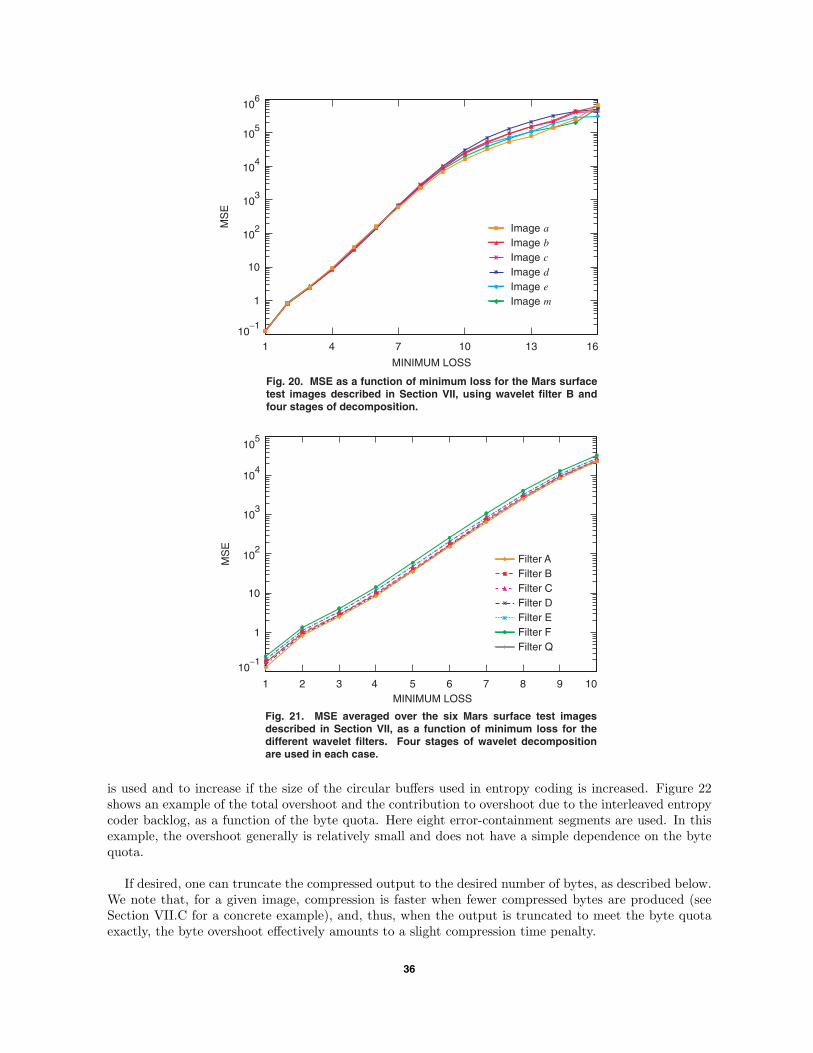
10

1

10-1

102

103

104

105

106

MINIMUM LOSS

MS

E

1 4 7 10 13 16

Image mImage eImage dImage cImage bImage a

Fig. 20. MSE as a function of minimum loss for the Mars surface test images described in Section VII, using wavelet filter B and four stages of decomposition.

10

1

1

10-1

102

103

104

105

MINIMUM LOSS

MS

E

2 3 4 5 6 7 8 9 10

Fig. 21. MSE averaged over the six Mars surface test images described in Section VII, as a function of minimum loss for the different wavelet filters. Four stages of wavelet decomposition are used in each case.

Filter QFilter FFilter EFilter DFilter CFilter BFilter A

is used and to increase if the size of the circular buffers used in entropy coding is increased. Figure 22shows an example of the total overshoot and the contribution to overshoot due to the interleaved entropycoder backlog, as a function of the byte quota. Here eight error-containment segments are used. In thisexample, the overshoot generally is relatively small and does not have a simple dependence on the bytequota.

If desired, one can truncate the compressed output to the desired number of bytes, as described below.We note that, for a given image, compression is faster when fewer compressed bytes are produced (seeSection VII.C for a concrete example), and, thus, when the output is truncated to meet the byte quotaexactly, the byte overshoot effectively amounts to a slight compression time penalty.

36

Flush ContributionTotal Overshoot

Fig. 22. Overshoot for 1024 ¥ 1024 Mars surface test image m , described in Section VII, using 8 segments, filter B, and 6 stages of wavelet decomposition. The target rate is the byte quota value converted to bits/pixel. The lower curve shows the contribution to overshoot due to flushing the interleaved entropy coder instances.

0.00

0.0

0.01

0.02

0.03

0.04

0.05

TARGET RATE, bits/pixel

OV

ER

SH

OO

T, b

its/p

ixel

0.5 1.0 1.5 2.0 2.5 3.0

Unfortunately, truncating the compressed output can result in a disparity in the reconstructed qualitiesof the various segments. This effect is due to the variation in the backlog of bits among the segments’interleaved entropy coders. If the average compressed data volume per segment is very small, the qualitydisparity between the segments can be quite noticeable.

During compression, ICER accumulates output sequentially, but because ICER compresses each error-containment segment of a subband bit plane before moving on to another subband bit plane, the outputbitstream interleaves data from the segments. Thus, a compressed segment consists of several blocks(generally one for each subband bit-plane segment plus a header block) that are interleaved in ICER’soutput. This organization of the output bitstream represents progressive compression across all of thesegments, and so is a convenient form from which to extract a specific number of compressed bytes.Thus, if truncation is needed to meet a storage or downlink constraint, one should truncate the overallcompressed data stream.

Figure 23(a) illustrates the arrangement of blocks of ICER compressed output that might arise whenICER compresses an image using three segments. In this example, ICER has produced a total of nineblocks; in a typical application, we might more realistically expect hundreds of blocks. Here segment 0consists of blocks a, d, and g; segment 1 consists of blocks b, e, and h; and segment 2 consists of blocks c,f , and i.

Whether or not truncation is performed, the compressed bitstream should be rearranged prior to trans-mission so that portions corresponding to a given segment are concatenated in order. This organizationhelps to minimize the impact of data loss by making it less likely that a single frame loss will affectmore than one segment; see Section V.A. Figure 23(b) illustrates the rearrangement of the compressedbitstream in conjunction with truncation to a byte limit. The location of boundaries between blocks isunimportant and need not be recorded once the blocks are arranged as in Fig. 23(b).

37

c fccc ff

b e h

a d g

(b)

Segment 0

Segment 1

Segment 2

c f icc iiffb e haBlock d g

SegmentIndex

(a)

Byte Limit

0 1 2 0 1 2 0 1 2

Fig. 23. Example of (a) ICER-compressed data output organization and (b) reorganization of compressed blocks following truncation to a byte limit.

VII. Results

In this section, we compare the lossy and lossless compression effectiveness of ICER to that of otherimage compressors and provide compression speed results for the MER implementation of ICER.

For our comparisons, we use six Mars surface images obtained from the Mars Pathfinder (MPF) missionImager for Mars Pathfinder (IMP) camera. As shorthand, we use a single letter identifier for each image.Images a through e are single-frame IMP images that were compressed losslessly onboard Mars Pathfinder;these can be obtained from the Planetary Data System (PDS).14 Image m is a mosaic of several single-frame IMP images, with a larger size (1024 × 1024) that matches the cameras onboard MER. All ofthe images have a bit depth of 12 bits/pixel. The image dimensions and MPF image identification (ID)numbers are listed in Table 11.

We evaluated the compression performance of ICER, JPEG 2000 [14], JPEG [31], LOCO [3–5], andtwo different Rice compressors [32]. ICER and JPEG 2000 provide lossless and lossy compression. JPEGprovides only lossy compression, and LOCO and Rice provide only lossless compression.

Table 11. MPF images used for evaluations.

MPF Size (W × H),Image

image ID pixels

a 0053140005 256 × 248

b 0182010121 256 × 248

c 0184010102 256 × 248

d 0182010070 256 × 248

e 0033030101 256 × 248

m (Mosaic) 1024 × 1024

14 Specifically, we obtained these images from the PDS Planetary Image Atlas for Mars Pathfinder IMP Images,http://www-pdsimage.jpl.nasa.gov/cgi-bin/MPF/MPF search.pl.

38

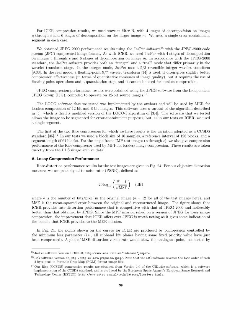
For ICER compression results, we used wavelet filter B, with 4 stages of decomposition on imagesa through e and 6 stages of decomposition on the larger image m. We used a single error-containmentsegment in each case.

We obtained JPEG 2000 performance results using the JasPer software15 with the JPEG-2000 codestream (JPC) compressed image format. As with ICER, we used JasPer with 4 stages of decompositionon images a through e and 6 stages of decomposition on image m. In accordance with the JPEG-2000standard, the JasPer software provides both an “integer” and a “real” mode that differ primarily in thewavelet transform stage. In the integer mode, JasPer uses a 5/3 reversible integer wavelet transform[9,33]. In the real mode, a floating-point 9/7 wavelet transform [34] is used; it often gives slightly bettercompression effectiveness (in terms of quantitative measures of image quality), but it requires the use offloating-point operations and a quantization step, and it cannot be used for lossless compression.

JPEG compression performance results were obtained using the JPEG software from the IndependentJPEG Group (IJG), compiled to operate on 12-bit source images.16

The LOCO software that we tested was implemented by the authors and will be used by MER forlossless compression of 12-bit and 8-bit images. This software uses a variant of the algorithm describedin [5], which is itself a modified version of the LOCO-I algorithm of [3,4]. The software that we testedallows the image to be segmented for error-containment purposes, but, as in our tests on ICER, we useda single segment.

The first of the two Rice compressors for which we have results is the variation adopted as a CCSDSstandard [35].17 In our tests we used a block size of 16 samples, a reference interval of 128 blocks, and asegment length of 64 blocks. For the single-frame IMP test images (a through e), we also give compressionperformance of the Rice compressor used by MPF for lossless image compression. These results are takendirectly from the PDS image archive data.

A. Lossy Compression Performance

Rate-distortion performance results for the test images are given in Fig. 24. For our objective distortionmeasure, we use peak signal-to-noise ratio (PSNR), defined as

20 log10

(2b − 1√MSE

)(dB)

where b is the number of bits/pixel in the original image (b = 12 for all of the test images here), andMSE is the mean-squared error between the original and reconstructed image. The figure shows thatICER provides rate-distortion performance that is competitive with that of JPEG 2000 and noticeablybetter than that obtained by JPEG. Since the MPF mission relied on a version of JPEG for lossy imagecompression, the improvement that ICER offers over JPEG is worth noting as it gives some indication ofthe benefit that ICER provides to the MER mission.

In Fig. 24, the points shown on the curves for ICER are produced by compression controlled bythe minimum loss parameter (i.e., all subband bit planes having some fixed priority value have justbeen compressed). A plot of MSE distortion versus rate would show the analogous points connected by

15 JasPer software Version 1.600.0.0, http://www.ece.uvic.ca/~mdadams/jasper/.16 IJG software Version 6b, ftp://ftp.uu.net/graphics/jpeg/. Note that the IJG software reverses the byte order of each

2-byte pixel in Portable Gray Map (PGM) format image files.17 Our Rice (CCSDS) compression results are obtained from Version 1.0 of the CID rice software, which is a software

implementation of the CCSDS standard, and is produced by the European Space Agency’s European Space Research andTechnology Center (ESTEC), http://www.estec.esa.nl/tech/datacwg/lossless.htmls.

39

PS

NR

, dB

20

30

40

50

60(a) (b)

PS

NR

, dB

20

30

40

50

60(c) (d)

RATE, bits/pixel

PS

NR

, dB

0 1 2 3 4 5 620

30

40

50

60(e)

RATE, bits/pixel

0 1 2 3 4 5 6

(f)

Fig. 24. Rate-distortion performance of ICER, real and integer modes of JPEG 2000, and JPEG on the test images: (a) image a , (b) image b , (c) image c , (d) image d , (e) image e , and (f) image m .

JPEGJPEG 2000, IntegerJPEG 2000, RealICER

approximately straight line segments, reflecting the sequential nature of the compression within bit planesof a given priority. Thus, when PSNR is plotted, the observed “scalloping” effect occurs. This effect isnot noticeable with JPEG 2000; two reasons for this are (1) in JPEG 2000 the multiple coding passeswithin a bit plane are designed so that bits coded in earlier passes give a larger reduction in distortionper compressed bit [13] and (2) the wavelet transforms used to obtain the JPEG 2000 results producefew bit planes with equal priorities.

40

B. Lossless Compression Performance

Table 12 gives the lossless compression performance on the 12-bit test images. In addition to losslesslycompressing 12-bit images, MER will also losslessly compress 8-bit images formed by quantizing the pixelsof 12-bit images. To illustrate lossless compression performance on 8-bit images, we produced an 8-bitversion of each test image by linearly scaling each pixel according to the minimum and maximum pixelvalues in the image to make full use of the 8-bit dynamic range. Table 13 lists the results.

We see that in terms of lossless compression effectiveness, ICER is comparable to LOCO; this is signif-icant because LOCO is a state-of-the-art compressor designed exclusively for lossless image compression.We also observe that ICER’s lossless compression effectiveness is superior to that of JPEG 2000 and theRice compressors, especially the Rice implementation used by the MPF mission.

C. Compression Speed

To provide a rough indication of compression speed, timing results were obtained for the MER im-plementation of ICER under the VxWorks operating system running on a 20-MHz RAD6000 processoridentical to those used by the MER rovers. Figure 25 contains a representative sample of the results. Thefigure demonstrates the fact that, for a given image, compression is faster when fewer compressed bytes

Table 12. Lossless compression performance on 12-bit images.

Rate, bits/pixelImage

ICER LOCO JPEG 2000 Rice (CCSDS) Rice (MPF)

a 8.19 8.15 8.48 8.63 9.38

b 8.90 8.92 9.24 9.39 10.13

c 9.08 9.10 9.43 9.66 10.21

d 9.40 9.41 9.74 9.93 10.61

e 8.76 8.83 9.11 9.23 9.87

m 8.36 8.62 8.59 9.34 n/a

Average 8.78 8.84 9.10 9.36 —

Table 13. Lossless compression performance on 8-bit images.

Rate, bits/pixelImage

ICER LOCO JPEG 2000 Rice (CCSDS)

a 4.72 4.63 4.86 5.07

b 4.99 4.94 5.17 5.40

c 5.45 5.41 5.67 5.95

d 5.76 5.71 5.98 6.21

e 4.83 4.79 5.00 5.23

m 4.40 4.62 4.64 5.26

Average 5.02 5.02 5.22 5.52

41

Filter Q Filter QFilter C Filter CFilter B Filter BFilter A Filter A

0

5

10

1.51.00.0 0.5

15

20

25

30

RATE, bits/pixel

CO

MP

RE

SS

ION

TIM

E, m

s/pi

xel

3 Decompositions 5 Decompositions

Fig. 25. ICER compression time on the 20-MHz RAD6000 processor used by the MER rovers, for test image m using one error-containment segment. Results courtesy of Todd Litwin, Jet Propulsion Laboratory, Pasadena, California.

are produced. The time to produce a compressed image at a bit rate of zero primarily reflects the timerequired to perform the wavelet decomposition of the image. Observe that the choice of wavelet filter ornumber of decompositions has little impact on compression speed.

VIII. Conclusion

The ICER image compressor was designed to meet the specialized needs of deep-space applications.ICER is wavelet-based and produces progressive compression, providing lossless and lossy compression,and incorporates an error-containment scheme to limit the effects of data loss on the deep-space chan-nel. ICER achieves state-of-the-art compression effectiveness, providing lossy compression performancecompetitive with the JPEG 2000 image compression standard, and lossless compression performance com-petitive with the LOCO image compressor. ICER noticeably outperforms the JPEG image compressorused by the MPF mission and provides significantly more effective lossless compression than the Ricecompressor used by that mission.

The MER mission, with a total of 18 cameras on two rovers, will rely heavily on ICER to enabledelivery of image data back to Earth during the 180 Martian days of surface operations. The MERmission is significantly advancing the state of practice of image compression for deep-space missions byusing image compressors that provide substantially more effective compression than that obtained by theMPF mission.

Rapid advances in imaging technologies will enable future missions to collect even higher volumes ofimage data and continue to push the need for innovative data compression technologies. We note somepossible improvements to ICER that would increase its functionality and effectiveness for future missions:

(1) Improvements to the overall compression effectiveness of ICER should be possible. Alikely avenue is to improve the context modeling and prediction during encoding of bitlayers by developing a more refined context modeler. Improvements in compressioneffectiveness would need to be balanced with complexity considerations.

42

(2) It would be fairly straightforward to modify ICER to provide more fine-grained controlover image-quality requests than currently supported by the minimum loss parameterdescribed in Section VI.A.

(3) The quality disparity that can occur when the bitstream is truncated and the overshoot ofthe byte quota (both discussed in Section VI.B) are two issues that are largely related tothe backlog of bits in each segment’s interleaved entropy coder. One straightforward wayof reducing the byte overshoot would be to estimate the backlog of bits in each segment’sinterleaved entropy coder when checking the byte quota. One also could periodically flusheach interleaved entropy coder, but this would reduce compression effectiveness slightly.A more integrated approach would involve changing the way that entropy coding isperformed.

(4) The decompressor could be modified to incorporate more sophisticated techniques forselecting quantizer reconstruction points than the current method of selecting a pointclose to the midpoint of each quantizer bin (see Section III.A). A thorough study ofthe distribution of subband data in typical images could yield an improved approach,perhaps by adaptively adjusting the quantizer reconstruction point based on observationsof nearby pixels. This would reduce distortion in the reconstructed image at a given bitrate without changing the compressor. Since the decompressor operates on the ground,fairly complex approaches could be considered.

Progressive compressors like ICER will enable future missions to employ sophisticated data-returnstrategies involving incremental image-quality improvements to maximize the science value of returneddata using an onboard buffer. Improvements in compression techniques and onboard hardware will allowfuture missions to reap larger benefits from image compression.

Acknowledgments

The authors would like to thank Justin Maki for providing information on MERand the use of ICER on MER. We thank Justin, Jim Bell, Steve Squyres, andothers on the MER mission team for their enthusiastic willingness to fly ICER eventhough it had not previously been used in space. Thanks are also due to ToddLitwin for providing ICER timing results. We gratefully acknowledge Todd, Justin,and Allan Runkle for providing information about image-compression techniquesused on the MPF mission. Finally, the authors would like to thank Sam Dolinarand Ken Andrews for several helpful technical discussions.

References

[1] S. Dolinar, A. Kiely, M. Klimesh, S. Shambayati, A. Ortega, S. Lee, P. Sagetong,H. Xie, and R. Manduchi, “Region-of-Interest Data Compression with Priori-tized Buffer Management (II),” Proceedings of the 2002 Earth Science TechnologyConference, paper PS2P2, Pasadena, California, June 11–13, 2002.

43

[2] J. N. Maki, J. F. Bell, K. E. Herkenhoff, S. W. Squyres, A. Kiely, M. Klimesh,M. Schwochert, T. Litwin, R. Willson, A. Johnson, M. Maimone, E. Baum-gartner, A. Collins, M. Wadsworth, S. T. Elliot, A. Dingizian, D. Brown,E. C. Hagerott, L. Scherr, R. Deen, D. Alexander, and J. Lorre, “The MarsExploration Rover Engineering Cameras,” Journal of Geophysical Research—Planets, vol. 108, no. E12, 8071, 2003 (in press).

[3] M. J. Weinberger, G. Seroussi, and G. Sapiro, “The LOCO-I Lossless ImageCompression Algorithm: Principles and Standardization into JPEG-LS,” IEEETransactions on Image Processing, vol. 9, no. 8, pp. 1309–1324, August 2000.

[4] M. J. Weinberger, G. Seroussi and G. Sapiro, “LOCO-I: A Low Complex-ity, Context-Based, Lossless Image Compression Algorithm,” Proceedings of theIEEE Data Compression Conference, pp. 140–149, 1996.

[5] M. Klimesh, V. Stanton, and D. Watola, “Hardware Implementation of a LosslessImage Compression Algorithm Using a Field Programmable Gate Array,” TheTelecommunications and Mission Operations Progress Report 42-144, October–December 2000, Jet Propulsion Laboratory, Pasadena, California, pp. 1–11,February 15, 2001.http://tmo.jpl.nasa.gov/tmo/progress report/42-144/144H.pdf

[6] A. Said and W. Pearlman, “Reversible Image Compression via MultiresolutionRepresentation and Predictive Coding,” Proceedings of the SPIE Conference onVisual Communications and Image Processing 1993, Cambridge, Massachusetts,Proc. SPIE, vol. 2094, pp. 664–674, November 1993.

[7] A. Said and W. A. Pearlman, “An Image Multiresolution Representation forLossless and Lossy Compression,” IEEE Transactions on Image Processing,vol. 9, no. 5, pp. 1303–1310, September, 1996.

[8] A. Zandi, A. D. Allen, E. L. Schwartz, and M. Boliek, “CREW: Compression withReversible Embedded Wavelets,” Proceedings of the IEEE Data CompressionConference, Snowbird, Utah, pp. 212–221, March 1995.

[9] M. D. Adams and F. Kossentini, “Reversible Integer-to-Integer Wavelet Trans-forms for Image Compression: Performance Evaluation and Analysis,” IEEETransactions on Image Processing, vol. 9, no. 7, pp. 1010–1024, June 2000.

[10] S. G. Mallat, “A Theory for Multiresolution Signal Decomposition: The WaveletRepresentation,” IEEE Transactions on Pattern Analysis and Machine Intelli-gence, vol. 11, no. 7, pp. 674–693, July 1989.

[11] J. M. Shapiro, “Embedded Image Coding Using Zerotrees of Wavelet Coeffi-cients,” IEEE Transactions on Signal Processing, vol. 41, pp. 3445–3462, De-cember 1993.

[12] A. Said and W. Pearlman, “A New, Fast, and Efficient Image Codec Based on SetPartitioning in Hierarchical Trees,” IEEE Transactions on Circuits and Systemsfor Video Technology, vol. 6, no. 3, pp. 243–250, June 1993.

[13] D. Taubman, “High Performance Scalable Image Compression with EBCOT,”IEEE Transactions on Image Processing, vol. 9, no. 7, pp. 1158–1170, July 2000.

[14] M. D. Adams, The JPEG-2000 Still Image Compression Standard, ISO/IEC JTC1/SC 29/WG 1 N 2412, September 2001.

[15] E. S. Hong, R. E. Ladner, and E. A. Risken, “Group Testing for Wavelet PacketImage Compression,” Proceedings of the IEEE Data Compression Conference,Snowbird, Utah, pp. 73–82, March 2001.

44

[16] A. B. Kiely, “Progressive Transmission and Compression of Images,” TheTelecommunications and Data Acquisition Progress Report 42-124, October–December 1995, Jet Propulsion Laboratory, Pasadena, California, pp. 88–103,February 15, 1996.http://tmo.jpl.nasa.gov/tmo/progress report/42-124/124E.pdf

[17] ISO/IEC, ISO/IEC 14492-1, Lossy/Lossless Coding of Bi-level Images, 2000.

[18] J. Rissanen and G. G. Langdon, “Arithmetic Coding,” IBM Journal of Researchand Development, vol. 23, no. 2, pp. 149–162, March 1979.

[19] L. Bottou, P. G. Howard, and Y. Bengio, “The Z-Coder Adaptive Binary Coder,”Proceedings of the IEEE Data Compression Conference, pp. 13–22, March 1998.

[20] P. G. Howard, “Interleaving Entropy Codes,” Proceedings Compression andComplexity of Sequences 1997, Salerno, Italy, pp. 45–55, 1998.

[21] A. B. Kiely and M. Klimesh, “A New Entropy Coding Technique for Data Com-pression,” The InterPlanetary Network Progress Report 42-146, April–June 2001,Jet Propulsion Laboratory, Pasadena, California, pp. 1–48, August 15, 2001.http://ipnpr.jpl.nasa.gov/tmo/progress report/42-146/146G.pdf

[22] A. B. Kiely and M. Klimesh, “Memory-Efficient Recursive Interleaved EntropyCoding,” The InterPlanetary Network Progress Report 42-146, April–June 2001,Jet Propulsion Laboratory, Pasadena, California, pp. 1–14, August 15, 2001.http://ipnpr.jpl.nasa.gov/tmo/progress report/42-146/146J.pdf

[23] F. Ono, S. Kino, M. Yoshida, and T. Kimura, “Bi-Level Image Coding withMELCODE—Comparison of Block Type Code and Arithmetic Type Code,”Proc. IEEE Global Telecommunications Conference (GLOBECOM ‘89),pp. 0255–0260, November 1989.

[24] K. Nguyen-Phi and H. Weinrichter, “A New Binary Source Coder and its Ap-plication to Bi-Level Image Compression,” Proc. IEEE Global Telecommunica-tions Conference (GLOBECOM ‘96), London, England, pp. 1483–1487, Novem-ber 1996.

[25] S. W. Golomb, “Run-Length Encodings,” IEEE Transactions on InformationTheory, vol. IT-12, no. 3, pp. 399–401, July 1966.

[26] R. G. Gallager and D. C. Van Voorhis, “Optimal Source Codes for Geometri-cally Distributed Integer Alphabets,” IEEE Transactions on Information The-ory, vol. IT-21, no. 2, pp. 228–230, March 1975.

[27] Consultative Committee for Space Data Systems, CCSDS 102.0-B-5: PacketTelemetry, Blue Book, issue 5, November 2000.http://www.ccsds.org/documents/102x0b5.pdf

[28] Consultative Committee for Space Data Systems, CCSDS 101.0-B-6: TelemetryChannel Coding, Blue Book, issue 6, October 2002.http://www.ccsds.org/documents/101x0b6.pdf

[29] R. McEliece and L. Swanson, “On the Decoder Error Probability for Reed-Solomon Codes,” IEEE Transactions on Information Theory, vol. 32, no. 5,pp. 701–703, September 1986.

[30] Consultative Committee for Space Data Systems, CCSDS 100.0-G-1: TelemetrySummary of Concept and Rationale, Green Book, issue 1, December 1987.http://www.ccsds.org/documents/100x0g1.pdf

45

[31] W. B. Pennebaker and J. L. Mitchell, JPEG Still Image Data Compression Stan-dard, Van Nostrand Reinhold, New York, 1993.

[32] R. F. Rice, Some Practical Universal Noiseless Coding Techniques, Part III,Module PSI14,K+, JPL-91-3, Jet Propulsion Laboratory, Pasadena, California,November 1991.

[33] A. R. Calderbank, I. Daubechies, W. Sweldins, and B.-L. Yeo, “Wavelet Trans-forms that Map Integers to Integers,” Applied and Computational HarmonicAnalysis, vol. 5, pp. 332–369, July 1998.

[34] M. Antonini, M. Barlaud, P. Mathieu, and I. Daubechies, “Image Coding us-ing Wavelet Transform,” IEEE Transactions on Image Processing, vol. 1, no. 2,pp. 205–220, April 1992.

[35] Consultative Committee for Space Data Systems, CCSDS 121.0-B-1: LosslessData Compression, Blue Book, issue 1, May 1997.http://www.ccsds.org/documents/121x0b1.pdf

46