The Goldstone Boson Higgs and the eective...

Ph.D. thesis

The Goldstone Boson Higgs and

the e�ective Lagrangian(s)

Candidate:

Kirill Kanshin

Universita‘ degli Studi di Padova

Dipartimento di Fisica e Astronomia “G. Galilei”

Scuola di Dottorato di Ricerca in Fisica

Via Marzolo 8, I-35131 Padova, Italy

Ciclo XXVIII

Advisor: Prof. Stefano Rigolin

Director of Ph.D. school: Prof. Andrea Vitturi

January 2017

Abstract

The Goldstone boson nature of the observed Higgs scalar particle represents a tempting possiblesolution for the Standard Model hierarchy problem. We first discuss the essence of the problem inthe context of low energy QCD and the Higgs sector of the Standard Model. As a step towardsthe solution we construct a UV complete model of the Goldstone Higgs based on the globalSO(5)/SO(4) symmetry breaking. The scalar sector of the theory is a linear sigma model extendedby a scalar singlet ‡, with mass m‡ > 500 GeV. In order to give mass to the SM fermions throughthe partial compositeness mechanism, the fermion sector is extended by heavy vectorlike fermions.We study in detail the possible direct detection of ‡ and the impact of the new scalar and fermionstates on Electroweak Precision Tests. We conclude in particular that any reasonable contributionof the scalar sector can in principle be compensated by a fermionic one. At low energies anyextension of the Standard Model results in a set of e�ective operators, describing the deviationsof the couplings from their predicted values. Depending on how the electroweak symmetry isrealised, two intrinsically di�erent e�ective descriptions are possible: linear and non-linear one.Varying the ‡ mass allows to sweep from the regime of the perturbative linear UV completion tothe non-linear one. The latter one is typically assumed in models in which the Higgs particle isa low-energy remnant of some strong dynamics at a higher scale. In the limit of large but finitemasses of the new states we derive the benchmark non-linear e�ective Lagrangian. Furthermorethe first order linear corrections originating from large, but finite mass of the additional scalarto the Higgs couplings have been derived and they are found to be suppressed by the scalarmasses ratio. Finally, we consider the renormalization of the custodial preserving scalar sectorof the non-linear e�ective Lagrangian in a general Goldstone bosons matrix parametrisation andidentify the physical counterterms as well as the chiral-noninvariant divergences. The latter onesare shown to be unphysical as they can be removed by a field redefinition. The procedure allowsto check the consistency of the non-linear e�ective Lagrangian at one loop. The results confirmthe completeness of the scalar sector of NLO Lagrangian previously identified in the literature.

Abstract

Una particella di Higgs la cui natura sia di tipo Goldstone rappresenta una possibile soluzione alproblema della gerarchia nel Modello Standard. Dapprima discutiamo l’essenza del problema nelcontesto della QCD di bassa energia e del settore di Higgs del Modello Standard. Come passosuccessivo verso la soluzione, si costruisce un modello UV-completo del Goldstone Higgs, basatosulla rottura di simmetria globale SO(5)/SO(4). Il settore scalare della teoria è un modello sigmalineare, esteso da un singoletto scalare ‡, con massa m‡ > 500 GeV. Per dare massa ai fermionidel Modello Standard attraveso il meccanismo di compositezza parziale, il settore fermionico vieneesteso da fermioni pesanti vectorlike. Si studia in dettaglio la possibile osservazione diretta di ‡ el’impatto del nuovo scalare e dei nuovi stati fermionici sui test di precisione elettrodeboli. Si con-clude, in particolare, che ogni ragionevole contributo dal settore scalare può , in linea di principio,essere compensato dal settore fermionico. A basse energie ogni estensione del Modello Standardrisulta in un insieme di operatori e�ettivi che descrivono le deviazioni dei coupling dai loro valoripredetti. A seconda di come la simmetria elettrodebole è realizzata, sono possibili due descrizionie�ettive intrinsicamente di�erenti: lineare e non lineare. Variando la massa dell’‡ passiamo concontinuità dal regime in cui il completamento è perturbativo a quello non lineare. Quest’ultimoè in genere un presupposto di modelli nei quali la particella di Higgs è un residuo a bassa en-ergia of dinamiche forti ad una scala superiore. Nel limite in cui le masse dei nuovi stati sonograndi, ma finite, deriviamo la Lagrangiana e�ettiva non lineare che può essere utilizzata comebenchmark. Inoltre vengono derivate le correzioni lineari al primo ordine causate dalla massa –grande ma finita – degli scalari addizionali ai coupling dell’Higgs, dimostrando che sono soppressedi un fattore proporzionale al rapporto degli scalari della teoria. Infine, consideriamo la rinormaliz-zazione del settore scalare che preserva la simmetria custodial in una parametrizzazione matricialedei bosoni di Goldstone e identifichiamo i controtermini fisici e le divergenze non-invarianti sottotrasformazioni chirali. Si dimostra che quest’ultime sono non fisiche, dal momento che possonoessere rimosse da una ridefinizione dei campi. La procedura consente di controllare la consistenzadella Lagrangiana e�ettiva non lineare a livello one-loop. I risultati confermano la completezza delsettore scalare della Lagrangiana NLO precedentemente identificata in letteratura.

Contents

Preface 4

1 Introduction 7

1.1 The Standard Model . . . . . . . . . . . . . . . . . . . . . . . . . . . . . . . . . . . 7

1.2 Goldstone bosons . . . . . . . . . . . . . . . . . . . . . . . . . . . . . . . . . . . . . 13

1.2.1 Pions as Pseudo-Nambu-Goldstone bosons in QCD . . . . . . . . . . . . . . 14

1.2.2 Higgs as Pseudo-Nambu-Goldstone boson in BSM . . . . . . . . . . . . . . . 24

1.3 E�ective Field Theory . . . . . . . . . . . . . . . . . . . . . . . . . . . . . . . . . . 30

1.3.1 SMEFT: Linear realisation of EW symmetry . . . . . . . . . . . . . . . . . . 33

1.3.2 HEFT: Nonlinear realisation of EW symmetry . . . . . . . . . . . . . . . . . 35

1.3.3 SMEFT vs. HEFT . . . . . . . . . . . . . . . . . . . . . . . . . . . . . . . . 39

2 The minimal linear sigma model for the Goldstone Higgs 41

2.1 The SO(5)/SO(4) scalar sector . . . . . . . . . . . . . . . . . . . . . . . . . . . . . 42

2.1.1 The scalar potential . . . . . . . . . . . . . . . . . . . . . . . . . . . . . . . 43

2.1.2 Scalar-gauge boson couplings . . . . . . . . . . . . . . . . . . . . . . . . . . 45

2.1.3 Renormalization and scalar tree-level decays . . . . . . . . . . . . . . . . . . 46

2.2 Fermionic sector . . . . . . . . . . . . . . . . . . . . . . . . . . . . . . . . . . . . . . 49

2.3 Phenomenology . . . . . . . . . . . . . . . . . . . . . . . . . . . . . . . . . . . . . . 53

2.3.1 Bounds from Higgs measurements . . . . . . . . . . . . . . . . . . . . . . . . 54

2.3.2 Precision electroweak constraints . . . . . . . . . . . . . . . . . . . . . . . . 55

2.3.3 Higgs and ‡ coupling to gluons . . . . . . . . . . . . . . . . . . . . . . . . . 62

2

2.3.4 Higgs and ‡ decay into ““ . . . . . . . . . . . . . . . . . . . . . . . . . . . . 66

2.4 The ‡ resonance at the LHC . . . . . . . . . . . . . . . . . . . . . . . . . . . . . . 69

2.5 d Æ 6 Fermionic E�ective Lagrangian . . . . . . . . . . . . . . . . . . . . . . . . . 72

3 The linear-non-linear frontier for the Goldstone Higgs 76

3.1 Model independent analysis . . . . . . . . . . . . . . . . . . . . . . . . . . . . . . . 77

3.1.1 Polar coordinates . . . . . . . . . . . . . . . . . . . . . . . . . . . . . . . . . 79

3.1.2 Expansion in 1/⁄ . . . . . . . . . . . . . . . . . . . . . . . . . . . . . . . . . 80

3.1.3 Impact on Higgs observables . . . . . . . . . . . . . . . . . . . . . . . . . . . 82

3.2 Explicit fermion sector . . . . . . . . . . . . . . . . . . . . . . . . . . . . . . . . . . 86

4 Non-linear EFT at one loop 90

4.1 The Lagrangian . . . . . . . . . . . . . . . . . . . . . . . . . . . . . . . . . . . . . . 91

4.1.1 The Lagrangian in a general U parametrisation . . . . . . . . . . . . . . . . 92

4.2 Renormalization of o�-shell Green functions . . . . . . . . . . . . . . . . . . . . . . 94

4.2.1 1-point functions . . . . . . . . . . . . . . . . . . . . . . . . . . . . . . . . . 96

4.2.2 2-point functions . . . . . . . . . . . . . . . . . . . . . . . . . . . . . . . . . 97

4.2.3 3-point functions . . . . . . . . . . . . . . . . . . . . . . . . . . . . . . . . . 99

4.2.4 4-point functions . . . . . . . . . . . . . . . . . . . . . . . . . . . . . . . . . 100

4.2.5 Dealing with the apparent non-invariant divergencies . . . . . . . . . . . . . 102

4.3 Renormalization Group Equations . . . . . . . . . . . . . . . . . . . . . . . . . . . . 103

4.4 Comparison with the literature . . . . . . . . . . . . . . . . . . . . . . . . . . . . . 104

Summary 106

A Coleman–Weinberg Potential 109

B The counterterms 111

C The Renormalization Group Equations 116

3

Preface

The electron is as inexhaustible as the atom, Nature is infinite, but it infinitely exists.And it is this sole categorical, this sole unconditional recognition of Nature’s existenceoutside the mind and perception of man that distinguishes dialectical materialism fromrelativist agnosticism and idealism.

– V.I. Lenin, Materialism and empirio-criticism, 1908

As more than 100 years have passed since the times of Lenin many more elementary particleshave been discovered with the famous Higgs boson being the last missing piece of the StandardModel (SM) – fundamental quantum field theory (QFT) of electromagnetic, weak and stronginteractions, describing with unprecedented precision the wide range of phenomena observed. Thediscovery of the Higgs boson [1, 2] completes the struggle for experimental verification of thisunifying description of the forces of Nature (all but gravity), yet it poses new theoretical challengesfor the upcoming generations of physicists. In this sense, though we seem to understand the theoryof the electron through Quantum Electrodynamics quite well, it is the physics of the Higgs bosonwhat seems to be inexhaustible nowadays and so the pursuit for the knowledge of infinite Naturecontinues.

One of the main theoretical challenges motivating to look for BSM physics is the so called hierar-chy problem. It can be stated as the failure of the SM to provide a theoretical explanation of therelatively light Higgs boson mass. From the QFT point of view the SM is a well defined, renor-malisable theory. However, it can be thought as an e�ective field theory, correctly describing thefundamental interactions at the energies accessible by modern experiments, but has to be extendedto include explanations of several theoretical puzzles, such as small neutrino masses, unobservedstrong CP angle, dark matter and dark energy being some of them. In addition, it cannot bethe ultimate theory since it does not include the description of gravity and is known to containa Landau pole for the electromagnetic coupling at very high energies. If the SM is treated as atheory valid up to some cut-o� scale �, any naive extension of the SM involving heavy states wouldintroduce quantum corrections of order ≥ �2 to the Higgs mass parameter. From this point ofview the observed value of the Higgs mass around the EW scale is unnaturally small and requiresa screening mechanism, stabilizing the Higgs mass at its observed value. Typically this requiresnew heavy BSM states in the vicinity of the electroweak scale.

On the other hand, the persistent absence of evidence for new resonances calls for an in-depthexploration of BSM theories which may separate and isolate the Higgs mass from the putative

4

scale of exotic BSM resonances. Several solutions have been proposed over decades, such assupersymmetry, compact extra dimensions, the relaxion mechanism and composite Higgs. Herewe will focus on the idea of the Higgs being a pseudo-Nambu-Goldstone boson (pNGB) of someglobal symmetry breaking, as was originally proposed decades ago in Refs. [3–8].

The first formulations of pNGB Higgs models were based on the assumption of a strong dynamicsobeying an SU(5) global group of symmetry broken down spontaneously to SO(5). The Higgswas identified with one of the NGB states of this breakdown. Recent attempts tend to start froma global SO(5) symmetry [9,10] at a high scale �, spontaneously broken to SO(4) and producingat this stage an ancestor of the Higgs particle. In [11,12] the next-to-minimal coset SO(6)/SO(5)with one more additional Goldstone boson (GB) been considered and studied as possible darkmatter candidate in [13,14].

In this thesis an explicit model of a pNGB Higgs based on SO(5)/SO(4) coset will be presented.While most of the literature uses an e�ective non-linear formulation of the models [10,15–21], weadopt the linear realization of the symmetry as suggested by [22]. See also [21] for the microscopicrealisation of the linear scalar sector in terms of Nambu-Jona-Lasino four-fermion interactions.More recent developments based on the idea of the linear scalar sector can be found in [23–27]. Thescalar sector of the theory is represented by a scalar multiplet in the fundamental representation ofSO(5) and contains the four SM scalar degrees of freedom plus an additional singlet ‡. This willallow to gain intuition on the dependence on the ultraviolet (UV) completion scale of the model,by varying the ‡ mass: a light ‡ particle corresponds to a weakly coupled regime, while in the largemass limit the theory should fall back onto a usual e�ective non-linear construction. Our completerenormalizable model can thus be considered either as an ultimate model made out of elementaryfields, or as a renormalizable version of a deeper dynamics, much as the linear ‡-model [28] is toQCD.

The fermion sector of the theory is extended by heavy vectorlike fermions forming complete repre-sentations under the SO(5) global group. The linear couplings between light and heavy fermionsallow for a see-saw like mechanism for quarks, whose masses are inversely proportional to theheavy fermion mass scale. This construction is known in the literature as the partial compos-iteness mechanism [29]. Many choices of the heavy fermions representations are available in theliterature, see Ref. [16] for a comparison between the possible options. The direction explored inthis work employs heavy fermions in vectorial and singlet representations of SO(5).

SO(5) breaking couplings of the heavy fermions to the SM ones together with proto-Yukawacouplings between scalar multiplet and heavy fermions allow for the generation of the GB Higgspotential. Its minimum breaks the electroweak symmetry at scale v and gives mass to Higgsparticle, massive gauge bosons and SM fermions.

Furthermore, we analyse the phenomenological implications of the modified scalar sector and theexotic fermions. In particular the contribution of the new sectors to the oblique S and T parameterswill be computed. We also study the possible LHC reach for the direct detection of the ‡ scalar,set a bound m‡ > 500 GeV and analyse its possible relation with the diphoton anomaly observedin 2014.

Next, we consequently integrate out the heavy states and identify the leading order e�ective

5

operators. Firstly, as the heavy fermions removed from the spectrum , we obtain a linear e�ectiveLagrangian composed of the Higgs, ‡ and SM fermions. Secondly, we integrate out the remainingscalar state, which results in the benchmark non-linear e�ective Lagrangian with the light Higgs,pointing out the leading contributions to the Higgs E�ective Field Theory (HEFT) operators.In addition we compute first linear corrections to the deviations of the Higgs to gauge bosonsand fermions (top and bottom) couplings and compare the results for di�erent heavy fermionsrepresentations.

Finally, we perform a complete one-loop o�-shell renormalization of the scalar sector of HEFT.While the previous literature has restricted the one-loop renormalization of this sector to on-shell analysis, the o�-shell renormalization procedure guarantees that all the counterterms neededare identified. We have obtained the explicit expressions for the chiral noninvariant divergencesobtained previously for the higgsless case and generalize it to the HEFT with the light Higgs. Wealso demonstrate that they vanish on-shell and have no impact on physical observables.

The structure of the thesis is as follows. Chapter 1 contains an introductory review of the topicscovered in the following chapters. In Chapter 2 we construct the renormalizable theory of thepNGB Higgs. In Chapter 3 we continue the study of the previously introduced model, switchingto the non-linear regime by integrating out the heavy scalar state. In Chapter 4 we study theone loop o�-shell renormalization of the scalar sector of HEFT. We conclude the thesis with aSummary.

Chapters 2-4 are based on publications [30–32].

6

1

Introduction

1.1 The Standard Model

The Standard Model (SM) of particle physics [33–35] is a model within the framework of QuantumField Theory (QFT), which has been proven to be a very precise description of the fundamental lawsof Nature. The discovery of a Higgs(-like) boson at LHC [1,2], predicted in milestone papers [36–39]and awarded by a Nobel Prize in Physics in 2013, concludes the continuous e�ort in constructingthe universal model describing the fundamental interactions of all known elementary particles andleaves us with a consistent framework allowing to reproduce the observed collider data.

The theory is based on the principles of gauge symmetry and renormalizability. In this section wewill introduce the quantum states of the theory and the symmetries which those quantum statesobey.

The postulated gauge symmetry imposed on the Lagrangian of the SM is

GSM = SU(3)c ◊ SU(2)L ◊ U(1)Y ,

where SU(3)c is the color symmetry, governing strong interactions of quarks and gluons, whileSU(2)L ◊ U(1)Y is the electroweak (EW) symmetry group – direct product of the chiral SU(2)group and the group of hypercharge, which is spontaneously broken at low energies and gives riseto weak and electromagnetic interactions. The gauge symmetry manifests itself in the invarianceof the Lagrangian under local (space-time dependent) gauge transformations which is assured bythe covariant derivatives of fields. Spin-1 gauge bosons form adjoint representations of the corre-sponding groups, while fermionic spin-1/2 fields are embedded into fundamental representationsof the groups.

The SM is a chiral theory, meaning that left- and right-handed fermion fields have di�erent trans-formation properties under the gauge group. This fact forbids the gauge non-invariant Dirac massterm for the SM fermions. The Higgs mechanism triggers the electroweak symmetry breaking(EWSB) and gives masses to quarks, charged leptons, W and Z bosons and the Higgs scalar itself.

The fermion sector consists of left-handed quarks qiL, transforming under the full GSM , right-

7

handed quarks ui and di transforming under SU(3)c ◊ U(1)Y , left-handed leptons li transformingunder the electroweak symmetry group and right-handed leptons ei charged only under U(1)Y .Both quarks and leptons come in three copies or generations, index i = 1, 2, 3 indicating that. Thecharge assignment for the SM fields is summarized in Table 1.1.

Fields Representation

Gauge

bosons

Bµ (1, 1, 0)

W aµ (1, 3, 0)

GAµ (8, 1, 0)

Quarksqi

L =31 uL

dL

2,1 cL

sL

2,1 tL

bL

22(3, 2, +1/6)

ui =1

u, c, t2

(3, 1, +2/3)

di =1

d, s, b2

(3, 1, ≠1/3)

LeptonsliL =

31 ‹eL

eL

2,1 ‹µ

L

µL

2,1 ‹·

L

·L

22(1, 2, ≠1/2)

ei =1

e, µ, ·2

(1, 1, ≠1)

Higgs H (1, 2, +1/2)

Table 1.1: Representations of the SM field content. Numbers in the brackets denote thedimension of the representation of SU(3)c, SU(2)L and charge under U(1)Y correspondingly.

The Lagrangian of the SM consists of the gauge, fermion and scalar sectors, and is written in termsof renormalizable operators up to dimension d = 4.

The gauge sector contains the invariant product of field strengths of the gauge bosons

Lgauge = ≠14Fµ‹F µ‹ ≠ 1

4W aµ‹W µ‹

a ≠ 14GA

µ‹Gµ‹A , (1.1)

where the field strength is

V µ‹A = ˆµV ‹

A ≠ ˆ‹V µA ≠ gfABCV µ

B V ‹C , (1.2)

where g is the coupling constant and fABC are the group structure constants, defined by a com-mutator of generators � of the group

[�A, �B] = ifABC�C .

The SU(2) generators read �a = ·a/2, where ·a are Pauli matrices, and the SU(3) generators are�A = ⁄A/2, with ⁄A being Gell-Mann matrices. Sign conventions vary in literature, Ref. [40]considers all possible sign conventions at once.

The fermionic sector contains the kinetic term and the Yukawa term, describing the Gauge–fermionand Higgs–fermion interactions correspondingly

Lf =ÿ

f=q,u,d

f iDµf ≠1(qi

LH) yijd d + (qi

LÊH) yij

u u + +(liLH) yij

e e + h.c.2

, (1.3)

8

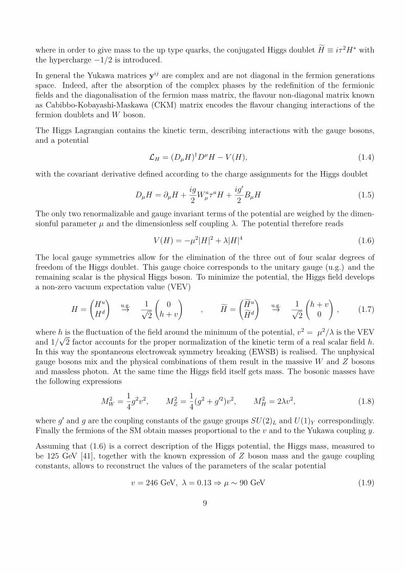
where in order to give mass to the up type quarks, the conjugated Higgs doublet ÊH © i· 2Hú withthe hypercharge ≠1/2 is introduced.

In general the Yukawa matrices yij are complex and are not diagonal in the fermion generationsspace. Indeed, after the absorption of the complex phases by the redefinition of the fermionicfields and the diagonalisation of the fermion mass matrix, the flavour non-diagonal matrix knownas Cabibbo-Kobayashi-Maskawa (CKM) matrix encodes the flavour changing interactions of thefermion doublets and W boson.

The Higgs Lagrangian contains the kinetic term, describing interactions with the gauge bosons,and a potential

LH = (DµH)†DµH ≠ V (H), (1.4)

with the covariant derivative defined according to the charge assignments for the Higgs doublet

DµH = ˆµH + ig

2 W aµ ·aH + igÕ

2 BµH (1.5)

The only two renormalizable and gauge invariant terms of the potential are weighed by the dimen-sionful parameter µ and the dimensionless self coupling ⁄. The potential therefore reads

V (H) = ≠µ2|H|2 + ⁄|H|4 (1.6)

The local gauge symmetries allow for the elimination of the three out of four scalar degrees offreedom of the Higgs doublet. This gauge choice corresponds to the unitary gauge (u.g.) and theremaining scalar is the physical Higgs boson. To minimize the potential, the Higgs field developsa non-zero vacuum expectation value (VEV)

H =A

Hu

Hd

Bu.g.æ 1Ô

2

A0

h + v

B

, ÊH =AÊHu

ÊHd

Bu.g.æ 1Ô

2

Ah + v

0

B

, (1.7)

where h is the fluctuation of the field around the minimum of the potential, v2 = µ2/⁄ is the VEVand 1/

Ô2 factor accounts for the proper normalization of the kinetic term of a real scalar field h.

In this way the spontaneous electroweak symmetry breaking (EWSB) is realised. The unphysicalgauge bosons mix and the physical combinations of them result in the massive W and Z bosonsand massless photon. At the same time the Higgs field itself gets mass. The bosonic masses havethe following expressions

M2W = 1

4g2v2, M2Z = 1

4(g2 + gÕ2)v2, M2H = 2⁄v2, (1.8)

where gÕ and g are the coupling constants of the gauge groups SU(2)L and U(1)Y correspondingly.Finally the fermions of the SM obtain masses proportional to the v and to the Yukawa coupling y.

Assuming that (1.6) is a correct description of the Higgs potential, the Higgs mass, measured tobe 125 GeV [41], together with the known expression of Z boson mass and the gauge couplingconstants, allows to reconstruct the values of the parameters of the scalar potential

v = 246 GeV, ⁄ = 0.13 ∆ µ ≥ 90 GeV (1.9)

9

The Higgs sector of the SM can be rewritten in a di�erent way, from which the global structure ofthe scalar sector can be seen more easily. Denoting the components of the doublet as („0, „1, „2, „3),the Higgs field and its conjugate before EWSB read

H = 1Ô2

A„2 + i„1„0 ≠ i„3

B

, H © i‡2Hú = 1Ô

2

A„0 + i„3

≠„2 + i„1

B

. (1.10)

The index assignment of the components of the doublet will become clear in the following. Wecan rewrite the Higgs sector of the SM, introducing a bidoublet notation

M(x) = „0(x) 1 + i„(x)· =A

„0 + i„3 „2 + i„1≠„2 + i„1 „0 ≠ i„3

B

©Ô

21H H

2(1.11)

where the latter notation stands for the matrix where the columns coincide with the componentsof the corresponding doublets. The scalar invariant can be obtained by taking the trace È. . . Í ofthe product of the M and its hermitian conjugate

12ÈM†MÍ = „2

0 + „2 (1.12)

The scalar potential rewritten in terms of bidoublet M(x) is similar to the one of the linear sigmamodel [28], which is discussed in greater details further on

V (M) = ⁄31

2ÈM†MÍ ≠ v242

. (1.13)

It obeys global SU(2)L ◊ SU(2)R symmetry with the following transformation property

M(x) æ LM(x)R†,

L = eila�a, R(x) = eira�a

,(1.14)

where la and ra are space-time independent parameters of the global transformations. The globalsymmetry of the scalar potential is violated explicitly by U(1)Y gauging and by the Yukawacouplings of the right-handed fermionic fields.

The local symmetry transformations can be embedded into the global SU(2)L ◊ SU(2). Indeed,taking into account that the hypercharges of H and ÊH are opposite in sign one can write thetransformation law under the local SU(2)L ◊ U(1)Y as following

M(x) æ L(x)M(x)R†3(x),

L(x) = eila(x)�a, R3(x) = eir3(x)�3

,(1.15)

where la(x) and r3(x) this time are space-time dependent parameters of the local transformations.The GSM covariant derivative reads

DµM(x) = ˆµM(x) + igW aµ �aM(x) ≠ igÕBµM(x) �3. (1.16)

10

In the bidoublet notation the Higgs sector of the SM is

L = 14ÈDµM†DµMÍ ≠ 1Ô

2(qLM Yq qR + lLM Yl lR + h.c.) ≠ V (M), (1.17)

Where flavour indexes are suppressed and right-handed doublets qR = (uR, dR), lR = (0, eR) withgeneralised Yukawa matrices have been introduced

Yq =A

yu 00 yd

B

, Yl =A

0 00 ye

B

. (1.18)

In the limit of gÕ æ 0 and yu = yd the global SU(2)L ◊ SU(2)R is exact. The vacuum state

ÈMÍ =A

v 00 v

B

, (1.19)

breaks the global symmetry down to vectorial subgroup SU(2)V which is also known as custodialsymmetry [42].

If only SU(2)L is gauged, the Higgs mechanism provides an equal mass to W and Z bosonsMW = MZ = gv/2, which reflects the fact that all the three gauge bosons belong to the triplet ofthe custodial symmetry group. The e�ect of the U(1)Y gauging results in the splitting betweenthe gauge bosons masses and can be characterised by a dimensionless parameter

fl = M2W

M2Z cos ◊W

, (1.20)

where cos ◊W = g/Ô

g2 + gÕ2. The custodial symmetry guarantees that at tree level the value of theparameter is fl = 1. In the SM it receives loop corrections proportional to the custodial violatingcoupling gÕ and to the di�erence between the Yukawa couplings of fermion doublets.

It is possible to introduce one more parametrisation of the scalar sector, the so called non-linearone. Consider the non-linear coordinate redefinition („0, „) æ (Ï, fi)

„0(x) æ Ï(x) cos (ifi(x)·/v) ,„(x)· æ Ï(x) sin (ifi(x)·/v) ,

∆ M(x) æ Ï(x) U(x), U(x) = eifi(x)·/v, (1.21)

The dimensionless object U(x) represents a matrix of would-be-Goldstone bosons of the Standardmodel. The field Ï(x) is a singlet under GSM , while all the transformation properties are carriedout by the matrix U(x)

Ï(x) æ Ï(x), U(x) æ L(x)U(x)R†3(x). (1.22)

Finally the Higgs potential V (Ï) = ⁄ (Ï2 ≠ v2)2 triggers EWSB, and the field Ï develops a VEVgiving rise to the physical Higgs boson

Ï æ h + v. (1.23)

11

Figure 1.1: Dominant SM contributions to Higgs mass parameter at one loop.

The Lagrangian after EWSB is rewritten accordingly

L = 12ˆµhˆµh + (h + v)2

4 ÈDµU†DµUÍ ≠ (h + v)Ô2

1qLU Yq qR + li

LU Yl lR + h.c.2

≠ V (h),

V (h) = 12m2

hh2 + ⁄vh3 + ⁄

4 h4.

(1.24)

With the covariant derivative defined in the same way as for M(x)

DµU(x) = ˆµU(x) + igW aµ �aU(x) ≠ igÕBµU(x) �3. (1.25)

The kinetic term of the would-be-Goldstone bosons accompanied by (h + v)2 in the unitary gaugeUU.G. = 1 provides the mass terms for the W and Z bosons, while the photon remains massless.

It is important to note that despite the fact that the scalar Lagrangian contains arbitrary highpowers of the fi fields, the SM remains renormalizable [43]: the non-linear field redefinition doesnot a�ect the property of renormalizability.

Hierarchy problem The parameters of the scalar sector of the SM with the values given inEq. (1.9) are the input parameters, reconstructed from the tree level expressions for the observables.At loop order they receive quantum corrections. The most relevant ones are of top quark (due tothe big value of yt), gauge bosons and Higgs boson loops, they all contain quadratically divergentcontributions and are not suppressed by a small coe�cient.

Assuming that the SM is an e�ective theory, which is valid only up to a cuto� energy scale �, thequantum corrections of the diagrams Fig 1.1 read [44]

1”µ(t)

22≥ ≠ 3

8fi2 y2t �2,

1”µ(g)

22≥ 1

16fi2 g2�2,

1”µ(H)

22≥ 1

16fi2 ⁄2�2.

(1.26)

The top quark loop numerically has the largest contribution and contributes negatively to the Higgsmass parameter, while the bosonic loops are smaller and contribute positively. The resulting massparameter at one loop reads:

µ2 = µ2tree +

ÿ

t,g,H

”µ2 (1.27)

12

Thus, for example for � = 10TeV, in order to obtain µ ≥ 100GeV, we need to set µtree ≥ 2TeVto cancel the contribution of the SM loops almost precisely. This fact is referred to as hierarchyproblem, which manifests itself in the large amount of fine-tuning required to obtain the observedvalue of the Higgs mass parameter [45]. The observed value of it is a small part of the contributiongenerated by the SM loops

µ2/ÿ

t,g,H

”µ2 ≥ 1% for � = 10 TeV. (1.28)

A smaller value of this ratio corresponds to a higher fine-tuning.

The clear way out of this problem is to lower the cuto� scale. Indeed for a lower cuto� the problemis not so dramatic and the fine-tuning is reasonable, for example

µ2/ÿ

t,g,H

”µ2 ≥ 25% for � = 1 TeV. (1.29)

Naively, the SM is valid all the way up to the Plank scale MP ≥ 1018 GeV . At this energy the e�ectsof quantum gravity are expected to become important. If there is no new physics responsible forthe Higgs mass generation and protection all the way up to MP , the tree level input parameter andthe quantum corrections would have to cancel with incredible precision of order µ2/”µ2 ≥ 10≠30.

Even if one rejects the cuto� argument used above (for example by using the scaleless regulariza-tion scheme, such as dimensional regularization [46], see Ref. [47]) the hierarchy problem can beunderstood as the unclear mechanism separating MP and EWSB scale v. There are strong theo-retical evidences that new physics must be present at lower scales in order to explain the origin ofneutrino masses, the strong CP problem and dark matter. Most of the solutions to the mentionedproblems require introduction of new heavy quantum states. If this is the case the masses of thosenew states will play the role of the cuto� scale � and in turn will introduce fine-tuning in thetheory, unless some mechanism protects the mass parameter from quantum corrections of all thestates in the extended theory.

The Higgs parameter thus is seen as unnaturally small. Following t’Hooft [48] the concept ofnaturalness can be formulated as follows: “A parameter can be naturally small only if setting it tozero increases the symmetry of the system”. In this case one says that the parameter is protected bythe symmetry. While a non-zero value of the parameter breaks the symmetry, quantum correctionswill be suppressed due to fact that the system obeys the approximate symmetry. The SM doesnot have any symmetry protecting the Higgs mass parameter.

One possible solution is that the Higgs might be a pseudo-Nambu-Goldstone boson (pNGB) of theglobal symmetry breakdown. In the following we will first discuss the properties of the GB in lowenergy QCD and then focus on the pNGB Higgs.

1.2 Goldstone bosons

In this section we are to describe the notion of Goldstone boson and then apply it to the cases ofpion physics and BSM physics. All the developed concepts will be then applied to construct thelinear sigma model for the Goldstone Higgs described in Chapters 2 and 3.

13

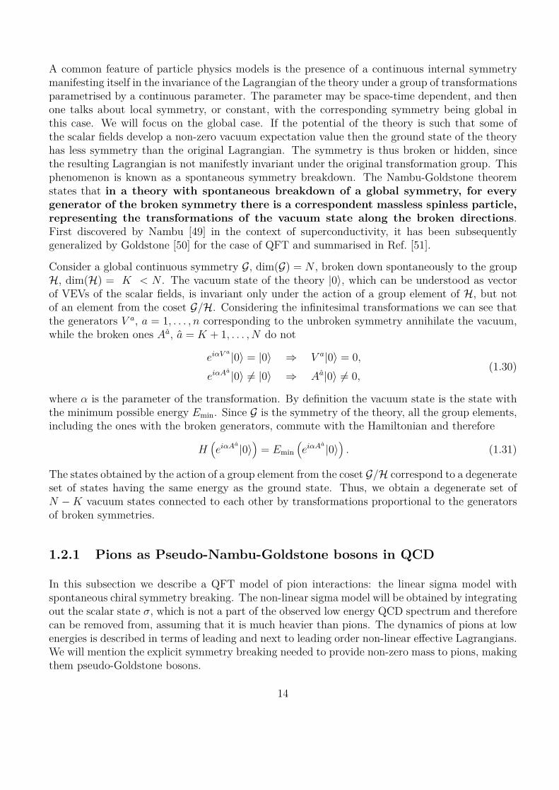
A common feature of particle physics models is the presence of a continuous internal symmetrymanifesting itself in the invariance of the Lagrangian of the theory under a group of transformationsparametrised by a continuous parameter. The parameter may be space-time dependent, and thenone talks about local symmetry, or constant, with the corresponding symmetry being global inthis case. We will focus on the global case. If the potential of the theory is such that some ofthe scalar fields develop a non-zero vacuum expectation value then the ground state of the theoryhas less symmetry than the original Lagrangian. The symmetry is thus broken or hidden, sincethe resulting Lagrangian is not manifestly invariant under the original transformation group. Thisphenomenon is known as a spontaneous symmetry breakdown. The Nambu-Goldstone theoremstates that in a theory with spontaneous breakdown of a global symmetry, for everygenerator of the broken symmetry there is a correspondent massless spinless particle,representing the transformations of the vacuum state along the broken directions.First discovered by Nambu [49] in the context of superconductivity, it has been subsequentlygeneralized by Goldstone [50] for the case of QFT and summarised in Ref. [51].

Consider a global continuous symmetry G, dim(G) = N , broken down spontaneously to the groupH, dim(H) = K < N . The vacuum state of the theory |0Í, which can be understood as vectorof VEVs of the scalar fields, is invariant only under the action of a group element of H, but notof an element from the coset G/H. Considering the infinitesimal transformations we can see thatthe generators V a, a = 1, . . . , n corresponding to the unbroken symmetry annihilate the vacuum,while the broken ones Aa, a = K + 1, . . . , N do not

ei–V a|0Í = |0Í ∆ V a|0Í = 0,

ei–Aa|0Í ”= |0Í ∆ Aa|0Í ”= 0,(1.30)

where – is the parameter of the transformation. By definition the vacuum state is the state withthe minimum possible energy Emin. Since G is the symmetry of the theory, all the group elements,including the ones with the broken generators, commute with the Hamiltonian and therefore

H1ei–Aa|0Í

2= Emin

1ei–Aa|0Í

2. (1.31)

The states obtained by the action of a group element from the coset G/H correspond to a degenerateset of states having the same energy as the ground state. Thus, we obtain a degenerate set ofN ≠ K vacuum states connected to each other by transformations proportional to the generatorsof broken symmetries.

1.2.1 Pions as Pseudo-Nambu-Goldstone bosons in QCD

In this subsection we describe a QFT model of pion interactions: the linear sigma model withspontaneous chiral symmetry breaking. The non-linear sigma model will be obtained by integratingout the scalar state ‡, which is not a part of the observed low energy QCD spectrum and thereforecan be removed from, assuming that it is much heavier than pions. The dynamics of pions at lowenergies is described in terms of leading and next to leading order non-linear e�ective Lagrangians.We will mention the explicit symmetry breaking needed to provide non-zero mass to pions, makingthem pseudo-Goldstone bosons.

14

Quantum Chromo Dynamics (QCD) is the fundamental theory of the strong interaction of quarksand gluons. It is a gauge theory based on the local SU(3)c group. At low energy it has the propertyof confining, meaning that colored objects – quarks, gluons or their non-color-neutral combinationscannot be observed separately in an experiment. Instead they form composite objects consisting ofmultiple (anti-)quarks. Historically the first observed composite objects of this type were protonsand neutrons – the constituents of the physical nuclei and therefore called nucleons.

Later on it was proposed by Yukawa [52] that nucleons stick together in the atom due to the strongnuclear force, with the force carrier being nearly degenerate in mass triplet of pions (fi0, fi±). Fromthe typical size of the atom it was possible to estimate the mass of the pions being of order 100MeV.

From the high energy perspective pions are understood as composite objects made of u and d (anti-)quarks, while from low energy they are seen as the pNGB of a global symmetry breaking. ThepNGB nature explains why pions are significantly lighter than all the other known QCD states.The global symmetry SU(2)L ◊ SU(2), called chiral symmetry, is dictated by the underlyingsymmetry of quasi-degenerate quark (u, d) doublet. It is broken down to the vectorial subgroupby spinless quark condensate developing a non-zero vacuum expectation value, ÈqLqÍ ”= 0, whichis not invariant under the whole chiral group. Inclusion of the additional strange quark, beingheavier than the other two, into a triplet of quarks (u, d, s) transforming under global flavourgroup SU(3)F accommodates for the additional pNGB states: 4 kaons and the ÷-meson, togetherwith pions forming an adjoint 8 representation of SU(3)F . In the following discussion we willrestrict ourselves to the case of pions only.

Linear ‡ - model

The linear sigma model is a phenomenological model constructed by Levi and Gell-Mann [28] todescribe the interaction of nucleons with pions.

Consider a doublet of nucleon fields consisting of proton and neutron fields

N =A

pn

B

. (1.32)

Even though those two states di�er by a unit of electrical charge, from a purely hadronic perspectivethey are very similar: they have almost the same mass mp = 938 MeV, (mn ≠ mp)/mn = 0.13%and are known to interact in a similar manner. Therefore in the limit of vanishing electroweakinteractions, the description of the states as a doublet is a good approximation. The kinetic partof the nucleon Lagrangian, written in terms of chiral fields ,

L = iNL /NL + iNR /NR, (1.33)

obeys a global chrial symmetry G = SU(2)L ◊ SU(2) under which the nucleon doublet transformsas

NL æ LNL, L = eila�a,

NR æ RNR, R = eira�a,

(1.34)

15

with la and ra being parameters of a global SU(2) transformations.

In infinitesimal form they can be rewritten as

”NL = ila�aNL,”NR = ira�aNR,

æ ”N = i(va ≠ aa“5)�aN, with va = (la + ra)/2,aa = (≠la + ra)/2.

(1.35)

where va, aa are the parameters of vectorial or isospin group transformation SU(2)V and axial orpure chiral transformation SU(2)A correspondingly.

If one naively attempts to introduce the mass term of the nucleon field this would break the axialsymmetry explicitly, leaving only the vectorial one. Indeed, the mass term is a cross term betweenleft and right chiral fields. Under SU(2)L ◊ SU(2) symmetry it transforms as

NLN æ NLe≠ila�aeirb�b

N (1.36)

For this to be invariant one has to put a constraint on the transformation parameters, la = ra,which corresponds to a smaller symmetry H = SU(2)V . Not to break axial symmetry explicitlybut instead spontaneously Gell-Mann and Levy introduced a bidoublet of scalar fields

M(x) = ‡(x) 1 + ifi(x)· , (1.37)

containing four scalar fields: singlet ‡ and triplet of pions fi. The chiral symmetry transformationreads

M æ LMR†. (1.38)Using the expression for the product of Pauli matrices ·a· b = ”ab1 + iÁabc·C the explicit transfor-mation properties of the field in infinitesimal limit are derived

”‡ = aafia, ”fia = ≠Áabcvbfic ≠ aa‡. (1.39)

The fields variations are linear functions of the non-transformed field. Therefore the chiral sym-metry is realised linearly on the set of scalar fields.

The renormalizable chiral invariant Lagrangian describes the nucleon-scalar system with the in-teraction strength parametrised by coupling constant g

L = iN /N + 14ÈˆµM†ˆµMÍ ≠ V (M) ≠ gNLMN ≠ gNM†NL, (1.40)

where the second term gives rise to kinetic terms of the scalar fields, V (M) is the scalar potentialand the last two terms describe the interaction of nucleons with the scalars, which in terms ofphysical fields can be written as

≠g‡NN ≠ igfiN“5·N. (1.41)

The second term of Eq. (1.41) describes the interaction of nucleons with the triplet of pseudoscalarpions which are indeed observed in QCD. Nevertheless this model does not meet yet the observa-tions for the following reasons:

1. Nucleons are known to have mass, but for the moment they remain massless. In order tointroduce nucleon masses spontaneous symmetry breaking has to occur.

16

2. The ‡ particle introduced previously is not exactly the state observed in QCD spectrum.Even though there is a state f0(500) with the appropriate quantum numbers (0++) it is verybroad and is barely seen in experiments. It is also about 5 times heavier than pions. We willintegrate out the ‡ particle from the spectrum and concentrate on the physics of pions only.This will lead to the non-linear ‡ - model.

3. Even though pions are decoupled from the heavy hadrons spectrum (mfi/mp ≥ 10%), theydo have a non-zero mass mfi ≥ 140 MeV. In order to introduce the pion mass an explicitsymmetry breaking is needed.

4. Multi-pion processes have been observed in the experiments, but the Lagrangian of the linear‡-model (1.40) does not contain any interactions between pions and has to be extended.

In the following we address each of these problems.

Spontaneous symmetry breaking: nucleon masses.

Lagrangian (1.40) does not contain a mass term for the nucleon field, but it does contain nucleon–scalar interactions and a scalar potential, which has not been specified yet. The mass can beobtained if one of the scalars obtains a non-zero VEV.

The potential is written in terms of scalar chiral invariants, such as12ÈM†MÍ = ‡2 + fi2. (1.42)

The trace of the product of higher number of M for the 2 ◊ 2 case is proportional to the samecombination ‡2 + fi2 [53]. There are only two d Æ 4 terms without derivative

d = 2 : ÈM†MÍ, (1.43)d = 4 : ÈM†MÍ2. (1.44)

Therefore the potential is parametrised by two independent coe�cients and can written as

V = ⁄1‡2 + fi2 ≠ F 2

22, (1.45)

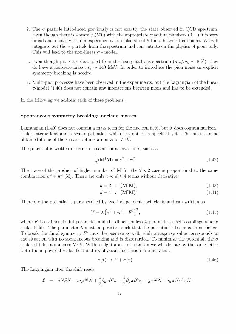
where F is a dimensionful parameter and the dimensionless ⁄ parametrises self couplings amongscalar fields. The parameter ⁄ must be positive, such that the potential is bounded from below.To break the chiral symmetry F 2 must be positive as well, while a negative value corresponds tothe situation with no spontaneous breaking and is disregarded. To minimize the potential, the ‡scalar obtains a non-zero VEV. With a slight abuse of notation we will denote by the same letterboth the unphysical scalar field and its physical fluctuation around vacua

‡(x) æ F + ‡(x). (1.46)

The Lagrangian after the shift reads

L = iN /N ≠ mNNN + 12ˆµ‡ˆµ‡ + 1

2ˆµfiˆµfi ≠ g‡NN ≠ igfiN“5·N ≠

17

λ

-F Fσ

V

Figure 1.2: Growing ⁄ shrinks the potential. The limit ⁄ æ Œ sets a restriction on thepotential and eliminates one degree of freedom.

≠ ⁄1‡2 + fi2

22≠ 4‡⁄F

1‡2 + fi2

2≠ 1

2m2‡‡2, (1.47)

where fermion and scalar masses are

mN = gF, m2‡ = 8⁄F 2. (1.48)

We can see that even though those masses are proportional to the same scale F they are controlledby two di�erent dimensionless parameters g and ⁄. Since these parameters are independent intheory the hierarchy between fermionic and scalar mass could be arbitrary.

The VEV of ‡ breaks the chiral symmetry SU(2)L ◊ SU(2) down to SU(2)V

ÈMÍ = F 1 æ LÈMÍR† = F (LR†) ∆ L = R ∆ aa = 0, (1.49)

while pions remain as massless degrees of freedom being Goldstone bosons associated to the threebroken generators of SU(2)A.

Since we disregarded isospin breaking e�ects the nucleons as well as pions masses are equal. Inthe following the isospin group SU(2)V will be considered an exact symmetry.

Non-Linear ‡-model.

The linear ‡-model is a renormalizable theory, accounting for the spontaneous chiral symmetrybreaking and describing pions as QCD Goldstone bosons (at the moment yet massless). We haveassumed that the object M(x) is a simple linear function of the fields ‡(x) and fi(x), such thatthey transform linearly under the chiral symmetry. As the ‡ particle has not been observed , 1 itcan be seen as an artefact of the mathematical apparatus used to construct the theory.

The most straightforward way to remove the ‡ scalar from the spectrum is to integrate it outassuming it is heavy. According to Eq. (1.48) in order to obtain m‡ æ Œ limit, while still keeping

1The observed 0++ state f0(500) has a very large width [54] and cannot be identified with the scalar of thelinear sigma model.

18

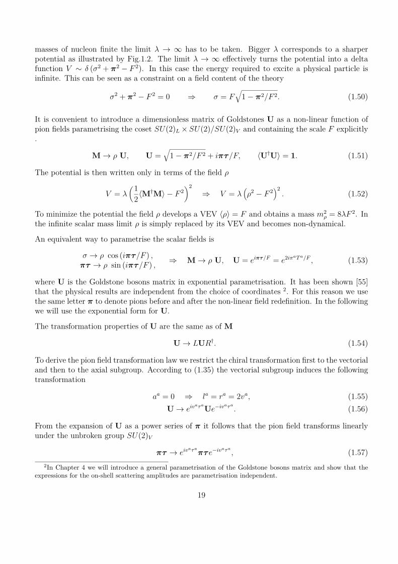
masses of nucleon finite the limit ⁄ æ Œ has to be taken. Bigger ⁄ corresponds to a sharperpotential as illustrated by Fig.1.2. The limit ⁄ æ Œ e�ectively turns the potential into a deltafunction V ≥ ” (‡2 + fi2 ≠ F 2). In this case the energy required to excite a physical particle isinfinite. This can be seen as a constraint on a field content of the theory

‡2 + fi2 ≠ F 2 = 0 ∆ ‡ = FÒ

1 ≠ fi2/F 2. (1.50)

It is convenient to introduce a dimensionless matrix of Goldstones U as a non-linear function ofpion fields parametrising the coset SU(2)L ◊ SU(2)/SU(2)V and containing the scale F explicitly.

M æ fl U, U =Ò

1 ≠ fi2/F 2 + ifi·/F, ÈU†UÍ = 1. (1.51)

The potential is then written only in terms of the field fl

V = ⁄31

2ÈM†MÍ ≠ F 242

∆ V = ⁄1fl2 ≠ F 2

22. (1.52)

To minimize the potential the field fl develops a VEV ÈflÍ = F and obtains a mass m2fl = 8⁄F 2. In

the infinite scalar mass limit fl is simply replaced by its VEV and becomes non-dynamical.

An equivalent way to parametrise the scalar fields is

‡ æ fl cos (ifi·/F ) ,fi· æ fl sin (ifi·/F ) ,

∆ M æ fl U, U = eifi·/F = e2ifiaT a/F , (1.53)

where U is the Goldstone bosons matrix in exponential parametrisation. It has been shown [55]that the physical results are independent from the choice of coordinates 2. For this reason we usethe same letter fi to denote pions before and after the non-linear field redefinition. In the followingwe will use the exponential form for U.

The transformation properties of U are the same as of M

U æ LUR†. (1.54)

To derive the pion field transformation law we restrict the chiral transformation first to the vectorialand then to the axial subgroup. According to (1.35) the vectorial subgroup induces the followingtransformation

aa = 0 ∆ la = ra = 2va, (1.55)U æ eiva·aUe≠iva·a

. (1.56)

From the expansion of U as a power series of fi it follows that the pion field transforms linearlyunder the unbroken group SU(2)V

fi· æ eiva·afi·e≠iva·a

, (1.57)2In Chapter 4 we will introduce a general parametrisation of the Goldstone bosons matrix and show that the

expressions for the on-shell scattering amplitudes are parametrisation independent.

19

while under the spontaneously broken group SU(2)A it transforms non-linearly

va = 0 ∆ ≠la = ra = 2aa, (1.58)U æ e≠iaa·aUe≠iaa·a (1.59)

(1 + ifi·/F + . . . ) æ (1 ≠ iaa·a + O(a2))(1 + ifi·/F + . . . )(1 ≠ iaa·a + O(a2)). (1.60)

Perturbatively the latter transformation can be written as

fia æ fia ≠ 2aaF + O(fi2), (1.61)

containing a constant shift of the pion field. This shift signals the spontaneous breaking of thecorrespondent symmetry and forbids the mass term for pions.

The non-linear sigma model is defined by the chiral invariant Lagrangian (1.40) in the limit ofinfinite scalar mass

L = iN /N + F 2

4 ÈˆµU†ˆµUÍ ≠ gFNLUN ≠ gFNU†NL. (1.62)

The potential has been eliminated by the restriction (1.50), promoting the heavy scalar field to benon-dynamical. The kinetic term of pions dictates higher order interaction terms, which can beread out expanding U in terms of physical fields

L ∏ 12ˆµfiˆµfi + 1

6F 2 (fiˆµfi)(fiˆµfi) ≠ 16F 2 (fifi)(ˆµfiˆµfi) + O(fi6) (1.63)

Linear corrections to the non-linear ‡-model

The restriction (1.50) corresponds to the exact ⁄ æ Œ limit. Keeping ⁄ large but finite and solvingperturbatively the equations of motion for the heavy scalar, one obtains the e�ective Lagrangiandescribing interactions of pions written as 1/⁄ expansion. In the following we demonstrate thee�ects of finite ⁄.

Disregarding the nucleon fields, the Lagrangian of the linear sigma model (1.40) in the exponentialparametrisation is rewritten as

L = 12ˆµflˆµfl + fl2

4 ÈˆµU†ˆµUÍ ≠ ⁄(fl2 ≠ F 2)2. (1.64)

The equation of motion for fl reads

⇤fl ≠ fl

2ÈˆµU†ˆµUÍ + 4⁄fl1fl2 ≠ F 2

2= 0. (1.65)

The perturbative solution up to the next to leading order in 1/⁄ expansion

fl = fl0 + fl1/⁄ + O(1/⁄2), (1.66)

20

results in the corresponding e�ective Lagrangian

L = L0 + L1/⁄ + O(1/⁄2). (1.67)

Solving the equation of motion for fl order by order we obtain

fl0 = F, (1.68)

fl1 = 116F

ÈˆµU†ˆµUÍ. (1.69)

Plugging these expressions back to the Lagrangian in addition to the pion kinetic term we obtainthe NLO correction [53]

L1 = ≠⁄32Ffl1

⁄

42= ≠ F 2

8m2‡

ÈˆµU†ˆµUÍ2, (1.70)

where we have traded ⁄ for the mass of the heavy scalar.

Explicit symmetry breaking: pion masses

The theory we have constructed up to now describes the interactions of massless pions, as thegroup G remains exact symmetry of the Lagrangian. Pions do have mass and therefore the chiralsymmetry has to be broken explicitly. In the underlying fundamental theory of pion interactions- QCD - it is the mass matrix of quarks what breaks the chiral symmetry. The rigorous way tointroduce pion masses in the context of non-linear QCD is through source fields, which will allowto track the explicit breaking of the symmetry. The sources are auxiliary fields, allowing for aformally chiral invariant Lagrangian. Fixing the values of source fields to non-dynamical valueswe will obtain the physical Lagrangian with massive pions.

Consider the simplest scalar source ‰ of canonical dimension d = 2 and promote it to have thefollowing transformation properties under the chiral symmetry

‰ æ R‰L† (1.71)

The only scalar invariant involving both GBs and source fields reads

d = 2 : È‰U† + U‰†Í. (1.72)

The Lagrangian of the non-linear sigma model with a scalar source then reads

L2 = F 2

4 ÈˆµU†ˆµUÍ + F 2

4 È‰U† + U‰†Í, (1.73)

where index 2 indicates the canonical dimension of the terms, disregarding the constant F .

Setting È‰Í = m2fi results in the mass term for pion

≠12m2

fififi + O(fi4). (1.74)

The pion mass term breaks the axial symmetry explicitly, while the vector one remains intact.

21

E�ective Lagrangian

Lagrangian (1.73) represents the minimal set of terms required to give an approximate descriptionof pion physics. This framework can be extended by the inclusion of higher dimensional termsd > 2. The general basis of d = 4 terms was first derived by Gasser and Leutwyler [56] and forthe case of SU(2) ◊ SU(2) chiral symmetry reads

L4 = –1ÈˆµUˆµU†Í2 + –2ÈˆµUˆ‹U†ÍÈˆµUˆ‹U†Í + (1.75)

+ –4ÈˆµUˆµU†ÍÈ‰U† + U‰†Í + –5È‰U† + U‰†Í2,

where –i are dimensionless coe�cients with measured values of order 10≠2 –10≠3.

To ensure the convergence of the expansion in canonical dimension the higher order terms haveto be suppressed by a scale �. Any additional power of the derivative or pion mass will be thenaccompanied by an inverse of the sale. To reveal the general counting scheme we rewrite the kineticterm in a symbolic form, omitting the numerical coe�cient and keeping track of scales

F 2�2A

ˆµ

� UB2

. (1.76)

Taking into account that each pion field is suppressed by F it is easy to estimate the contributionof any vertex with Nfi pion fields originating from this term

F 2�2A

ˆ

�

B2 Afi

f

BNfi

. (1.77)

Generalizing this result to Np powers of derivatives and Nm mass insertions the counting formulareads [57,58]

F 2�2A

ˆ

�

BNp 3mfi

�

4NmA

fi

f

BNfi

. (1.78)

To estimate the relative weight between the Lagrangians with two and four derivatives we willfocus on the fifi æ fifi scattering. Each derivative corresponds to a characteristic energy of theprocess ˆ ≥ E. Using the counting formula Eq. (1.78) the contributions read

L2 : (ˆ2fi4) æ E2

F 2 , (1.79)

L4 : (ˆ4fi4) æ E2

�2E2

F 2 . (1.80)

The contribution of four-derivative term is suppressed by a factor (E/�)2 and can be neglectedat low energies E π �. Thus, the expansion in "derivatives" (both space-time derivative andmass are counted the same) allows for a more precise description, taking into account the (E/�)corrections to the leading order (LO) Lagrangian with two derivatives. This expansion is knownas chiral perturbation theory and can be summarised as

L = L2 + L4 + . . . . (1.81)

22

The expansion above is valid all the way up to the energies E = �, at which all the terms givecontributions of the same order and the expansion breaks down.

Now consider loop corrections to the tree level 4fi scattering amplitude. Computing the e�ects ofvirtual particles at one loop with the LO Lagrangian vertexes results in

Lloop2 æ

3E

4fiF

42 E2

F 2 (fin + div), (1.82)

where "finite" is the dimensionless finite part of the amplitude, "div" denotes the infinite termextracted for example by dimensional regularisation and the 4fi coe�cient is the result of loopmomentum integration. This divergence is proportional to four powers of energy and cannot bereabsorbed by the leading order terms, L4 counterterms are required instead. Thus, higher orderterms in the chiral expansion are needed for the consistency of the chiral perturbation theory atloop level. The validity of the loop expansion requires the loop contribution to be subdominantto the tree level one, which is true for E < 4fiF .

Assuming that the tree level NLO contribution is compatible with the loop contribution or larger

F 2

�2 Ø 116fi2 (1.83)

we obtain the famous relation [58]

� Æ 4fiF. (1.84)

External gauging

Using the language of external sources it is possible to introduce also the SM gauge fields W and Zby gauging the electroweak group. Pions are composed of particles charged under SU(2)L ◊U(1)Y

and therefore they participate in those interactions as well. Under U(1)em, embedded into theunbroken SU(2)V , pions form a triplet (fi≠, fi0, fi+). We omit the details here and will mentionseveral properties of the gauged non-linear sigma model.

• Leptonic decays of pions. The pion is the lightest hadron and remains stable if electroweakinteractions are switched o�. Turning on the EW interaction allows for leptonic decay ofcharged pion fi+ or fi≠ predominantly into µ+‹µ or µ≠‹µ correspondingly, with branchingratio ≥ 99%. The Goldstone boson scale enters in the expression for the matrix element ofquark axial current È0|jµ

5 |fi≠(p)Í = iFpµ with jµ5 = 1Ô

2 u“µ“5d , parametrizing the hadronicpart of the decay amplitude and consequently in the pion lifetime [59]. It is identified withthe pion decay constant F = 93 MeV.

• Di�erence of masses of fi± and fi0. The quark composition of charged and neutral pionsis di�erent. Electromagnetic interactions violate the SU(2)V symmetry, generate a pionpotential and introduce a small splitting between the masses of pions (mfi+≠mfi0)/mfi+ ≥ 3%.

23

Under the assumption that the dominant contribution to pion form factors comes from thefirst heavy meson resonances fl and a1 (so-called vector dominance) the splitting reads [60]

m2fi± ≠ m2

fi0 ƒ 3–em

4fi

m2flm2

a1

m2a1 ≠ m2

fl

logA

m2a1

m2fl

B

∆ mfi± ≠ mfi0 ≥ 5.8MeV (1.85)

which is in good agreement with experimental value mfi± ≠ mfi0 ƒ 4.6 MeV.It is interesting too see that assuming that the splitting is controlled by a cuto� � ≥ 4fiFwe can estimate the mass splitting purely from the dimensional analysis as

m2fi± ≠ m2

fi0 ƒ –em

4fi(4fiF )2 ∆ mfi± ≠ mfi0 ≥ 8.8 MeV (1.86)

• Massive W ± and Z. QCD vacuum state breaks chrial invariance and therefore it breakselectroweak symmetry down to U(1)em, a situation completely analogous to the SM itself,with the only di�erence that there is no physical scalar obtaining the VEV. The pions areeaten to form longitudinal polarisations of W and Z bosons and therefore the gauge bosonsobtain masses [45]

mW = gF

2 ƒ 29 MeV, mZ = gF

2 cos ◊Wƒ 33 MeV. (1.87)

The values obtained are by 3 orders smaller than the real ones, though the important obser-vation that the strong dynamics is able to provide a mass to the gauge bosons has led to theidea of technicolor and consequently to Composite Higgs models.

1.2.2 Higgs as Pseudo-Nambu-Goldstone boson in BSM

One possible solution to the hierarchy problem is to promote the physical Higgs boson to bea pseudo-Nambu-Goldstone boson of a global symmetry breaking. In this case, on dimensionalanalysis grounds the Higgs mass parameter does not receive corrections from arbitrary high scalesof the BSM theory, but instead only from the global symmetry breaking scale multiplied by theexplicit symmetry breaking parameters. While still some fine-tuning is typically required, theGoldstone Higgs option represents a tempting possibility for the new physics and will be discussedin details in what is following.

A peculiar feature of pNGB Higgs is the split spectrum – the Higgs, being the lightest state of thenew sector, is significantly lighter than all the other new states and in the limit of the unbrokenglobal symmetry remains precisely massless. Thus the non-observation of the new states at scalev is thus naturally explained, while the typical scale of new heavy states is lifted up to a few TeV.

Finally, all the known scalar particles, with the possible exception of the QCD ‡≠meson, areunderstood as (pseudo-)Goldstone bosons, such is the case for pions, discussed in the previoussection or the longitudinal polarisations of W and Z.

24

Technicolor

The idea of technicolor models [45,61,62] being to a large extent the upscaled version of QCD wasproposed long before the experimental discovery of the Higgs boson and exhibited no massive scalarin the spectrum, reproducing only the Goldstone bosons of the SM and predicting heavy resonancesaround TeV scale. As in QCD the Lagrangian of the model is invariant under chiral symmetrygroup with NTC, flavours SU(NTC) ◊ SU(NTC), broken down spontaneously to SU(NTC)V bycondensate of (techi-)quark-antiquark pairs. The technipion decay constant FTC = 246 GeV , asdictated by the expression for the SM gauge bosons masses Eq. (1.87) , is analogous to the piondecay constant of QCD FQCD = 93 MeV. Scaling up the mass of the first resonance in QCD andassuming for simplicity that the number of colors is not so di�erent from the three colors of QCDwe can estimate the mass of techi-fl meson as

flTC ≥ FTC

FQCDmfl ≥ 2 TeV. (1.88)

The original technicolor models encountered serious phenomenological problems and were eventu-ally ruled out. Even before the Higgs discovery severe constrains were posed on the parameters ofthe models.

• Flavour changing neutral currents (FNCN). In the absence of the Higgs mechanismproviding mass to the SM quarks, to generate mass term for the light quarks both QCDand TC are embedded in a larger Extended Technicolor (ETC) group [63, 64], broken downspontaneously at high scale �ETC

SU(NETC) æ SU(3)c ◊ SU(NTC) (1.89)

This in turn produces a set of heavy gauge bosons with the mass of order �ETC. The exchangeof the heavy bosons generate four-fermion operators, suppressed by the gauge boson mass.As techiquarks condensate, the mixed light-heavy operators lead to an e�ective mass termfor the SM quarks

mq ƒ g2ETC

�2ETC

(qq)ÈÂTCÂTCÍ ƒ �TC

A�TC

�ETC

B2

. (1.90)

For �TC = v = 245 GeV the strange quark mass sets �ETC ≥ 10 TeV. Moreover, to reproducethe hierarchy of the quark masses the SU(NETC) breaking scale has to be di�erent for eachquark flavour. The group has to undergo series of hierarchical breakings, at di�erent scalesfor each quark, inversely proportional to their masses.On the other hand the SM four-fermion operators are suppressed by the same scale as mixedones and in general violate both CP and flavour

g2ETC

�2ETC

(qq)(qq) (1.91)

The experimental bound �ETC > 105 TeV does not allow to reproduce the observed lightquarks masses and therefore this set-up is ruled out.

25

• Electroweak Precision Tests (EWPT) It has been shown that in the Large N approx-imation that the contribution of the techicolor sector to Peskin–Takeuchi parameter S isapproximately [65–67]

S ≥ NT CNT D

fi, (1.92)

where NT D is the number of technidoublets. Even for the small number of colors and flavoursthe contribution is S ≥ 1, which is ruled out by EWPT performed at LEP.

The Composite Higgs as Nambu-Goldstone boson

Technicolor has been a motivation for a more elaborated idea of composite Higgs [3–8], being aninterpolation between the strongly interacting non-linear picture and the weakly interacting SMHiggs. Complete reviews of the topic can be found in [68, 69]. As in technicolor or QCD, in thecomposite Higgs framework one assumes a strongly interacting sector obeying a global symmetryG at high energies of order � ≥ 1 TeV, with a zoo of composite resonances forming completerepresentations of the group. At low energies it is broken spontaneously to a smaller group H.The scale of the breaking f is analogous to the pion decay constant F at which the chiral symmetryof the low energy QCD is broken. The Goldstone bosons resulting from the breaking must includeboth the longitudinal degrees of freedom of the SM gauge bosons and the Higgs boson itself,produced firstly as an exact massless GB. The coset G/H has to be large enough in order toinclude all the four degrees of freedom. For example for the most simple choices of special unitaryand orthogonal groups this means

SU(N)/SU(N ≠ 1) ∆ (2N ≠ 1) GB ∆ N Ø 3, (1.93)SO(N)/SO(N ≠ 1) ∆ (N ≠ 1) GB ∆ N Ø 5. (1.94)

The original Georgi-Kaplan model [5] relies on the SU(5)/SO(5) coset. Later the minimal com-posite Higgs (MCHM) model was proposed [9,10], based on the SO(5)/SO(4) symmetry breakingand containing exactly 4 GBs. In [70] the e�ective operators produced from the cosets of the the-ories above, as well as the minimal intrinsically custodial violating coset SU(3)/(SU(2) ◊ U(1)),have been derived. In [11] the next-to-minimal coset SO(6)/SO(5) with one more additional GBwas considered. It has been studied as possible dark matter candidate in [13,14].

The typical way to include the SM gauge group and its subsequent breaking can be described asa three step process

1. At scale � the theory is invariant under the global group G, broken down spontaneously togroup H at the scale f . This breaking produces n = dim(G) ≠ dim(H) Goldstone bosons.

2. The Standard Model gauge group GSM is embedded into the unbroken group H. The Higgsboson is one of the Goldstone bosons originating from the G/H breaking, transforming underthe GSM . Since the Higgs is an exact Golstone boson at tree level there are no potentialterms and therefore GSM remains unbroken.

26

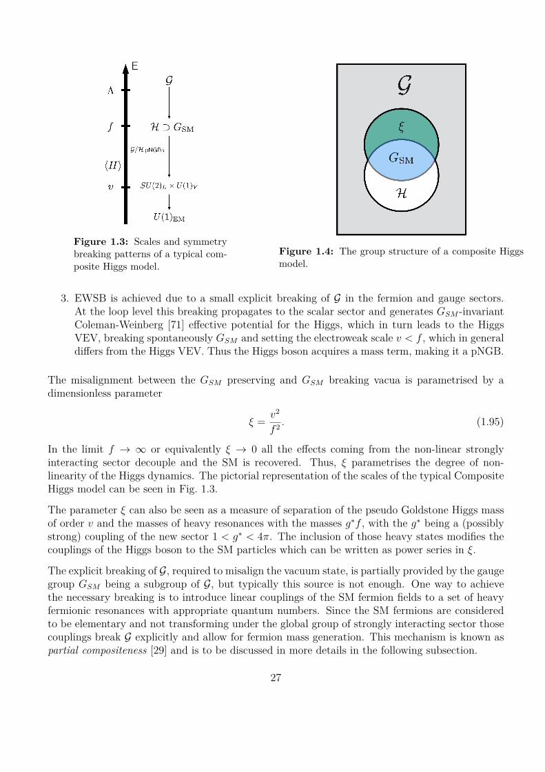
Figure 1.3: Scales and symmetrybreaking patterns of a typical com-posite Higgs model.

Figure 1.4: The group structure of a composite Higgsmodel.

3. EWSB is achieved due to a small explicit breaking of G in the fermion and gauge sectors.At the loop level this breaking propagates to the scalar sector and generates GSM -invariantColeman-Weinberg [71] e�ective potential for the Higgs, which in turn leads to the HiggsVEV, breaking spontaneously GSM and setting the electroweak scale v < f , which in generaldi�ers from the Higgs VEV. Thus the Higgs boson acquires a mass term, making it a pNGB.

The misalignment between the GSM preserving and GSM breaking vacua is parametrised by adimensionless parameter

› = v2

f 2 . (1.95)

In the limit f æ Œ or equivalently › æ 0 all the e�ects coming from the non-linear stronglyinteracting sector decouple and the SM is recovered. Thus, › parametrises the degree of non-linearity of the Higgs dynamics. The pictorial representation of the scales of the typical CompositeHiggs model can be seen in Fig. 1.3.

The parameter › can also be seen as a measure of separation of the pseudo Goldstone Higgs massof order v and the masses of heavy resonances with the masses gúf , with the gú being a (possiblystrong) coupling of the new sector 1 < gú < 4fi. The inclusion of those heavy states modifies thecouplings of the Higgs boson to the SM particles which can be written as power series in ›.

The explicit breaking of G, required to misalign the vacuum state, is partially provided by the gaugegroup GSM being a subgroup of G, but typically this source is not enough. One way to achievethe necessary breaking is to introduce linear couplings of the SM fermion fields to a set of heavyfermionic resonances with appropriate quantum numbers. Since the SM fermions are consideredto be elementary and not transforming under the global group of strongly interacting sector thosecouplings break G explicitly and allow for fermion mass generation. This mechanism is known aspartial compositeness [29] and is to be discussed in more details in the following subsection.

27

The GB degrees of freedom can be represented by a matrix

�(x) = ei�(x)/f , (1.96)

where � = �a(x)Aa, the vector �a(x) is the set of Goldstone bosons of G/H breaking and Aa asbefore denotes the generators of broken symmetries, a = 1 . . . dim(G/H), V a are the generators ofthe unbroken symmetry group H, a = 1 . . . dim(H).

The matrix � is a group transformation corresponding to the G/H coset. The action of an arbitrarygroup element g œ G on � parametrises another group element gÕ œ G, as it follows from the closureproperty of the group product operation. Since every group element of G can be decomposed asa product of a broken and unbroken symmetry transformation, which we denote as �Õ and hcorrespondingly, the following decomposition is valid

g �(x) = gÕ = �Õ(x)h(g, �) (1.97)

Therefore the matrix � has the following transformation properties [72, 73]

�(x) æ �Õ(x) = g �h≠1(g, �). (1.98)

If the global group G allows for an automorphism g æ g = R(g), with

R : Aa æ ≠Aa, (1.99)

the GB matrix transformation law can be recast as

�(x) æ �Õ(x) = h(g, �) �g≠1. (1.100)

It is immediate to see that the squared GB matrix obeys a simple transformation law

U(x) = �(x)2 = e2i�(x)/f , UÕ = gUg≠1. (1.101)

This form has been used previously for the low energy QCD and will be used in the followingdiscussion of the Electroweak Chiral Lagrangian in section 1.3.2.

Fermions and partial compositeness

The strongly coupled sector of the composite Higgs models typically includes a set of compositeheavy fermionic resonances �, forming complete representations under the global group of symme-try G. The elementary fermions of the SM, to which we will refer as light ones, instead transformonly under the gauge group GSM. In the simplest case of vectorlike heavy fermions, the mass termM�L� can be introduced straightforwardly and is invariant under G. To provide mass for theSM quarks and leptons the couplings between the elementary and composite fermions have to beconsidered. In technicolor this has been achieved through the e�ective nonrenormalizable bilinearcouplings (1.90), which led to severe phenomenological problems. The alternative idea proposedin Ref. [29] employs linear couplings of the light fermions q and operators originating from the

28

strongly coupled sector, such as � itself. The couplings violate explicitly the global group G andcan be formally written as

L ∏ �L (qL �q≠�) � + � �L (��≠q q) + h.c., (1.102)

where �q≠� (��≠q) are the spurion fields connecting GSM and G representations (and vice versa),while �L/R are dimensionful couplings. The latter ones can be made much smaller than the scaleof composite resonances by the RG evolution, thus reproducing the hierarchy for the SM quarkmasses.

The heavy fermions representations under G are not defined uniquely and introduce a strong modeldependence in the phenomenological results. Multiple possible embeddings of the heavy fermionsfor the MCHM and their impact on phenomenology have been analysed in [16].

Provided that proto-Yukava coupling between the heavy fermions and composite Higgs state isallowed and parametrised by Y , the explicitly G-breaking couplings �L/R propagate to the scalarsector at loop level and generate the CW potential for the Higgs, which eventually triggers EWSB.

The mixing between heavy and light fermions together with EWSB characterized by the scale v,result in the see-saw like expression for the light SM fermions, with the Yukawa coupling being afunction of the parameters of the strongly interacting sector

mq ≥ y v, y = Y�L

M

�M

. (1.103)

The ratios �L/R/M characterize the degree of mixing between the fermions. Only the heaviest topquark has a significant admixture of the composite state, while the other light quarks are mostlyelementary.

Other models of Goldstone Boson

Above we have briefly outlined the idea of the strong dynamics at high energies leading to thecomposite Higgs as a composite pseudo Goldstone boson.

The complementary concept of the pNGB Higgs is a Little Higgs model, originally proposed in [74]and further studied in [75], see [76] for a review. The Little Higgs construction does not necessarilyrely on strong dynamics at high energies and instead assumes perturbative regime at scales aroundTeV. The additional 5th space dimension is deconstructed and represented by a discrete numberof sites. The 4D symmetry is extended into the five dimensions, which in the deconstructed spaceresults in a direct product of multiple copies of the gauge groups living in the di�erent sites. TheHiggs boson seen as a fifth component of the 5D gauge field becoming a GB of the collectivebreaking of the global symmetries. Due to the collective nature of the breaking the quadraticdivergences are suppressed by the product of the breaking parameters, such that fine-tuning isreasonable.

The descriptions above implement the e�ective description of the Golstone boson degrees of free-dom and therefore are written typically in terms of e�ective and therefore non-renormalizable

29

Lagrangian [72, 73]. While this does not pose a big problem for the calculability of observables,renormalizable, UV complete underlying theories are considered in the literature.

One possible direction to go is to consider a microscopic UV completion, the dynamics of particlesforming the bound states at energies around TeV scale. Depending on the particular choice of therank of the new gauge group and the number of colors, either through lattice simulations or frompurely group theoretical considerations, it is possible to restrict the emerging global symmetrygroup and its breaking pattern. This eventually will allow for the determination of preferablecosets and define the number of emerging Goldstone bosons. Following this program [77, 78]analysed several possible gauge theories leading to SU(5)/SO(5) and SU(4)/Sp(4) cosets. Thelatter breaking pattern has been also analysed in Ref. [79], as the one emerging from the minimalstrongly interacting theory consisting of and SU(2) gauge group with two Dirac fermions in thefundamental representation.

Another way to construct a renormalizable theory is to promote the Higgs boson to be a partof a complete G representation, transforming linearly under the global group. The completionof the multiplet requires the existence of new scalar degrees of freedom. Ref. [12] considered anelementary realisation of pNGB Higgs for SU(4)/Sp(4) ≥ SO(6)/SO(5) coset. In the simplest caseof SO(5)/SO(4) linear model the spectrum is extended by one electroweak singlet scalar. In thecontext of the Goldstone Higgs this set up has been first mentioned first [22] and consequently [17].More detailed phenomenological study of the additional scalar, perspectives for the direct detection,impact of the extended fermionic sector on EWPT and the e�ective field theory resulting from theintegrating out the new degrees of freedom have been conducted in [31, 32] and will be discussedin details in Chapters 2,3. Furthermore, UV complete linear realisations of the global symmetryhave been considered in [23–27].

1.3 E�ective Field Theory

Though numerous theories have been proposed in the literature, dealing with the hierarchy problemand more generally with challenges of the current understanding of what the complete theory ofparticle physics should be, the parameter space of the possible extensions of the SM model issomewhat overwhelming. In order to confirm or disprove a theory in hand one can directly calculatethe expressions for the possible observables and compare them with the available measurementsof these observables provided by experiments. This procedure, known as the top-down approach,is a possible way, but due to the large number of the New Physics theories, if one is interestedin considering various possible models it is not e�ective. The more e�ective way involves the useof E�ective Field Theories as a tool making possible the study of all the theories at once or - ifsome additional assumptions are made - whole classes of BSM extensions. Once the observablesare expressed in terms of the parameters of the EFT, a given UV theory can be matched into theEFT, resulting in relations among its (otherwise free) parameters and this way it can be eithervalidated or disproved.

The construction of the EFT within QFT can be performed considering the following steps

30

1. Physical scales. Whether one studies the beta decay of neutron or performs EWPTs atLEP it is always possible to define the characteristic scale of the problem E, being for examplethe momentum transfer between the initial and final state.

2. Particle content. The next step requires identification of the relevant degrees of freedom interms of quantum fields. Fortunately, to study the interactions at the given scale one does notneed to know the complete theory of everything up to infinite energies [80]. This has alwaysbeen the case and it is very hard to imagine any progress in physics otherwise. Therefore theheavy (much heavier than the typical scale of interactions under study) or simply unknowndegrees of freedom can be neglected and not included explicitly in the Lagrangian.

3. Symmetries. The third step consists of imposing the physical symmetries. Thus, trans-formation properties under Lorentz group will define scalar, fermion, vectorial and possiblyhigher spin fields, while the internal symmetries with the proper charge assignments willfurther restrict the possible interaction terms.

4. Counting. Finally, in order to distinguish among more and less important e�ects, andpossibly take into account the subleading contributions to the modifications of interactions, a small parameter has to be defined. The Lagrangian of the EFT can be expressed as apower series of such parameter. The famous decoupling theorem [80] states that in a localquantum theory with some light particles with mass m . E interacting with a particle ofmass M ∫ E, the Green functions with only light particles as external legs can be obtainedsimply by omitting the heavy particles, up to the corrections of inverse powers of M . Thedimensionless expansion parameter in this case is E/M . In the following we will activelyexploit this fact, assuming that the new physics is represented by heavy states.

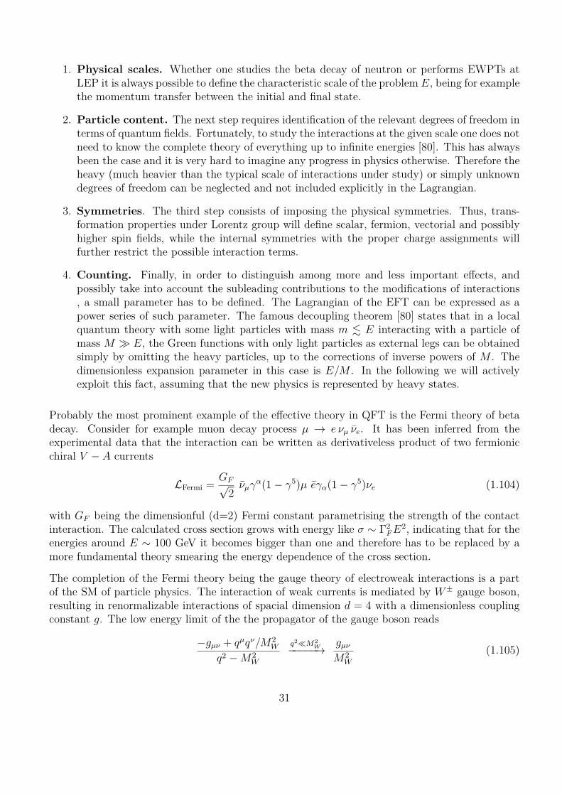
Probably the most prominent example of the e�ective theory in QFT is the Fermi theory of betadecay. Consider for example muon decay process µ æ e ‹µ ‹e. It has been inferred from theexperimental data that the interaction can be written as derivativeless product of two fermionicchiral V ≠ A currents

LFermi = GFÔ2

‹µ“–(1 ≠ “5)µ e“–(1 ≠ “5)‹e (1.104)

with GF being the dimensionful (d=2) Fermi constant parametrising the strength of the contactinteraction. The calculated cross section grows with energy like ‡ ≥ �2

F E2, indicating that for theenergies around E ≥ 100 GeV it becomes bigger than one and therefore has to be replaced by amore fundamental theory smearing the energy dependence of the cross section.

The completion of the Fermi theory being the gauge theory of electroweak interactions is a partof the SM of particle physics. The interaction of weak currents is mediated by W ± gauge boson,resulting in renormalizable interactions of spacial dimension d = 4 with a dimensionless couplingconstant g. The low energy limit of the the propagator of the gauge boson reads

≠gµ‹ + qµq‹/M2W

q2 ≠ M2W

q2πM2W≠≠≠≠≠æ gµ‹

M2W

(1.105)

31

The approximate momentum independent expression justifies the use of the Lagrangian (1.104)and allows to identify the expression of the Fermi constant in terms of the parameters of the SM

GFÔ2

= g2

8M2W

(1.106)

Further expansion of the bosonic propagator as powers of q2/M2W determines the corrections to

the Fermi Lagrangian.

Another example of e�ective Lagrangian has been described before considering the low energyQCD Lagrangian – non linear sigma model of pion interactions. Theoretically it can be seen eitheras a power series of operators, sorted according to the small parameter E/�QCD, or as a lowenergy limit of the UV complete model – linear sigma model. The first point of view on the chiralLagrangian of QCD turned out to be correct, while the parameters of the e�ective Lagrangianobtained from the integrating out heavy ‡ fields do not match physically measured values.

Finally, there are good reasons to believe that the SM itself is an e�ective theory. Being the mostsuccessful theory of fundamental interactions it yet does not address some key issues, such asdark matter, neutrino masses, the strong ◊ angle and eventually it does not provide the quantumdescription of gravity. One typically assumes that the physics resolving and explaining all theseissues will be accompanied by new heavy states which have not been yet observed, since the e�ectof their interaction is suppressed by some high scale �.

The use of the E�ective Theories for BSM models have been summarised in [81] and can be seenas three step process (see also the original Fig.1.5)

1. Given the UV model at high scales � the parameters or the Wilson coe�cients ci(�) of theEFT can be calculated. This step is called matching of UV completion into the EFT.

2. In general, the UV completion may be well separated in energy scale with the di�erence beingof orders of magnitude. In this case the running e�ects are relevant and in order to match thelow energy observables the running coe�cients with “ij – the anomalous dimensions matrixhave to be computed.

3. Finally, the coe�cients of the EFT are run down to the EW scale ci(mW ). The observablesare to be computed at this scale and compared to the predictions of the UV completions.This is mapping.

This is a general plan to proceed towards the construction of the EFT for the study of BSM e�ects.The particle content will include all the known elementary particles discovered, thus coincidingwith the particle content of the SM.

Furthermore, we will rely on Lorentz symmetry and gauge symmetries of the SM, exploring onlydeviations from the SM preserving GSM. Any BSM theory compatible with the symmetries as-sumed can be projected down into the set EFT operators. GSM can be realised either linearlyor non-linearly leading to two intrinsically di�erent e�ective theories. The linear realisation asit is the case for the SM itself and generally for the weakly coupled BSM models such as super-symmetry corresponds to scenarios in which the Higgs belongs to an elementary SU(2)L doublet

32

Figure 1.5: Connection between UV completion and the e�ective theory at EW scale [81].

and commonly known as Standard Model E�ective Field Theory (SMEFT) or linear EFT. Thenon-linear case is preferable for strongly interacting theories or for the theories with Goldstoneboson origin of the Higgs as is shown in Chapter 3. It corresponds to the case where all thegauge transformation properties are carried out by the would-be-Goldstones of the SM, while thephysical higgs boson is a complete singlet under GSM and therefore might enter through polyno-mial functions of the physical Higgs field. This scenario is known as Higgs E�ective Field Theory(HEFT) or electroweak chrial Lagrangian (EWChL) resembling the chiral Lagrangian of the lowenergy QCD. Both approaches are perfectly viable and we will consider them separately in thefollowing subsections, where we introduce the building blocks for both, discuss power counting foreach case and demonstrate LO and NLO e�ective Lagrangians. For an extensive overview of thetopic see also CERN "Handbook of LHC Higgs Cross Sections 4" [82].

1.3.1 SMEFT: Linear realisation of EW symmetry

Assuming that the BSM physics is weakly coupled and well separated from the SM, it can berepresented by a cuto� scale � being for example the mass of the lightest BSM state. TheLagrangian of the linear EFT can be written simply as power series on �. Assuming in additionlepton and baryon number conservation, the lowest order correction is suppressed by two powersof cuto� scale

Llinear = LSM +ÿ

i

ci

�2 Oi + O3 1

�4

4. (1.107)

The set of operators Oi of spacial dimension 6 represent linear independent basis parametrisingcorrections to the SM Lagrangian originating from the BSM physics, preserving the symmetriesassumed. Giving up the lepton number symmetry, there is only one d = 5 operator of the form(lH)2 providing Majorana mass term for the neutrinos and thus violating the lepton number by

33

X3 H6 and H4D2 Â2H3

QG fABCGA‹µ GBfl

‹ GCµfl QH (H†H)3 QeH (H†H)(lpeH)

QÂG fABC ÂGA‹µ GBfl

‹ GCµfl QH⇤ (H†H)⇤(H†H) QuH (H†H)(qpuÊH)

QW ÁabcW a‹µ W bfl

‹ W cµfl QHD

1H†DµH

2ú 1H†DµH

2QdH (H†H)(qpdH)

Q ÂW Áabc ÊW a‹µ W bfl

‹ W cµfl

X2H2 Â2XH Â2H2D

QHG H†H GAµ‹GAµ‹ QeW (l‡µ‹e)·aHW a

µ‹ Q(1)Hl (H†i

¡Dµ H)(l“µl)

QH ÂG H†H ÂGA

µ‹GAµ‹ QeB (l‡µ‹e)HBµ‹ Q(3)Hl (H†i

¡D I

µ H)(l·a“µl)

QHW H†H W aµ‹W aµ‹ QuG (q‡µ‹⁄Au)ÊH GA

µ‹ QHe (H†i¡Dµ H)(e“µe)

QH ÂW H†H ÊW a

µ‹W aµ‹ QuW (q‡µ‹u)·a ÊH W aµ‹ Q(1)

Hq (H†i¡Dµ H)(q“µq)

QHB H†H Bµ‹Bµ‹ QuB (q‡µ‹u)ÊH Bµ‹ Q(3)Hq (H†i

¡D I

µ H)(q·a“µq)

QH ÂB H†H ÂBµ‹Bµ‹ QdG (q‡µ‹⁄Ad)H GA

µ‹ QHu (H†i¡Dµ H)(u“µu)

QHW B H†·aH W aµ‹Bµ‹ QdW (q‡µ‹d)·aH W a

µ‹ QHd (H†i¡Dµ H)(d“µd)

QH ÂW B

H†·aH ÊW aµ‹Bµ‹ QdB (q‡µ‹d)H Bµ‹ QHud i(ÊH†DµH)(u“µd)

Table 1.2: Dimension-six operators with up to two fermion fields in Warsaw basis.

two units, �L = 2 [83]. The fact that this operator violates the accidental symmetry of the SMcan be related to a bigger suppression scale �. Therefore operators of d = 6, preserving all thesymmetries of the SM, are expected to give more significant contributions.

The building blocks for the e�ective operators are the SM fields and their functions, which arecovariant under GSM : H – Higgs field transforming linearly under GSM, the covariant derivativesDµ, the field strengths of the gauge bosons Vµ‹ and its dual Vµ‹ = Áµ‹fl‡Vfl‡ and finally the fermionicquark and lepton fields.

The exact form of the basis is not uniquely defined since it can be changed by applying theEquations of Motions (EOM) derived from the d = 4 Lagrangian to the d = 6 operators and byintegration by parts. The choice of the basis in each particular study is motivated by the set ofphenomenological processes one is planning to analyse, nonetheless since they all represent thebasis of operators, di�erent choices of it have the same phenomenological consequences [84].

The complete basis of d = 6 operators was obtained for the first time by Buchmuller et al. inRef. [85]. Further on, some modifications of this basis have been proposed in [86]. Ref. [87] proposeda linear basis under assumption of the pNGB Higgs originating from strong dynamics and finallyGrzadkowski et al [88] have removed the redundancies of Buchmuller et al. basis obtaining 59independent baryon number conserving operators. The latter is also known as Warsaw basis. Thelist of the linear bosonic and two fermion operators in the Warsaw basis is given in Table 1.2, while

34

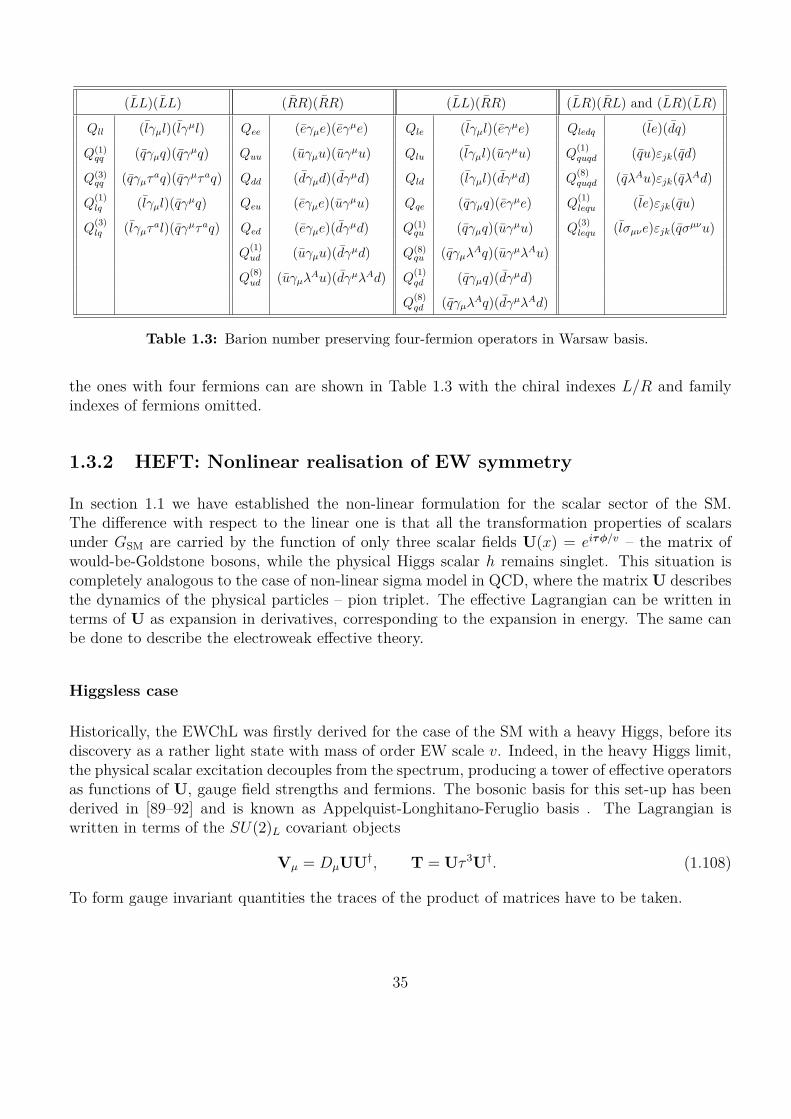
(LL)(LL) (RR)(RR) (LL)(RR) (LR)(RL) and (LR)(LR)

Qll (l“µl)(l“µl) Qee (e“µe)(e“µe) Qle (l“µl)(e“µe) Qledq (le)(dq)

Q(1)qq (q“µq)(q“µq) Quu (u“µu)(u“µu) Qlu (l“µl)(u“µu) Q(1)

quqd (qu)Ájk(qd)

Q(3)qq (q“µ·aq)(q“µ·aq) Qdd (d“µd)(d“µd) Qld (l“µl)(d“µd) Q(8)

quqd (q⁄Au)Ájk(q⁄Ad)

Q(1)lq (l“µl)(q“µq) Qeu (e“µe)(u“µu) Qqe (q“µq)(e“µe) Q(1)

lequ (le)Ájk(qu)

Q(3)lq (l“µ·al)(q“µ·aq) Qed (e“µe)(d“µd) Q(1)

qu (q“µq)(u“µu) Q(3)lequ (l‡µ‹e)Ájk(q‡µ‹u)

Q(1)ud (u“µu)(d“µd) Q(8)

qu (q“µ⁄Aq)(u“µ⁄Au)

Q(8)ud (u“µ⁄Au)(d“µ⁄Ad) Q(1)

qd (q“µq)(d“µd)

Q(8)qd (q“µ⁄Aq)(d“µ⁄Ad)

Table 1.3: Barion number preserving four-fermion operators in Warsaw basis.

the ones with four fermions can are shown in Table 1.3 with the chiral indexes L/R and familyindexes of fermions omitted.

1.3.2 HEFT: Nonlinear realisation of EW symmetry

In section 1.1 we have established the non-linear formulation for the scalar sector of the SM.The di�erence with respect to the linear one is that all the transformation properties of scalarsunder GSM are carried by the function of only three scalar fields U(x) = ei·„/v – the matrix ofwould-be-Goldstone bosons, while the physical Higgs scalar h remains singlet. This situation iscompletely analogous to the case of non-linear sigma model in QCD, where the matrix U describesthe dynamics of the physical particles – pion triplet. The e�ective Lagrangian can be written interms of U as expansion in derivatives, corresponding to the expansion in energy. The same canbe done to describe the electroweak e�ective theory.

Higgsless case

Historically, the EWChL was firstly derived for the case of the SM with a heavy Higgs, before itsdiscovery as a rather light state with mass of order EW scale v. Indeed, in the heavy Higgs limit,the physical scalar excitation decouples from the spectrum, producing a tower of e�ective operatorsas functions of U, gauge field strengths and fermions. The bosonic basis for this set-up has beenderived in [89–92] and is known as Appelquist-Longhitano-Feruglio basis . The Lagrangian iswritten in terms of the SU(2)L covariant objects

Vµ = DµUU†, T = U· 3U†. (1.108)

To form gauge invariant quantities the traces of the product of matrices have to be taken.

35

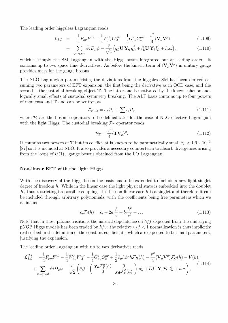
The leading order higgsless Lagrangian reads

LLO = ≠14Fµ‹F µ‹ ≠ 1

4W Aµ‹W µ‹

A ≠ 14Ga

µ‹Gµ‹a ≠ v2

4 ÈVµVµÍ + (1.109)

+ÿ

Â=q,u,d

ÂiDµÂ ≠ vÔ2

1qLU Yq qj

R + liLU Yl lj

R + h.c.2

, (1.110)

which is simply the SM Lagrangian with the Higgs boson integrated out at leading order. Itcontains up to two space time derivatives. As before the kinetic term of ÈVµVµÍ in unitary gaugeprovides mass for the gauge bosons.

The NLO Lagrangian parametrising the deviations from the higgsless SM has been derived as-suming two parameters of EFT expansion, the first being the derivative as in QCD case, and thesecond is the custodial breaking object T. The latter one is motivated by the known phenomeno-logically small e�ects of custodial symmetry breaking. The ALF basis contains up to four powersof momenta and T and can be written as

LNLO = cT PT +ÿ

ciPi. (1.111)where Pi are the bosonic operators to be defined later for the case of NLO e�ective Lagrangianwith the light Higgs. The custodial breaking PT operator reads

PT = v2

4 ÈTVµÍ2. (1.112)

It contains two powers of T but its coe�cient is known to be parametrically small cT < 1.9 ◊ 10≠3

[87] so it is included at NLO. It also provides a necessary counterterm to absorb divergences arisingfrom the loops of U(1)Y gauge bosons obtained from the LO Lagrangian.

Non-linear EFT with the light Higgs

With the discovery of the Higgs boson the basis has to be extended to include a new light singletdegree of freedom h. While in the linear case the light physical state is embedded into the doubletH, thus restricting its possible couplings, in the non-linear case h is a singlet and therefore it canbe included through arbitrary polynomials, with the coe�cients being free parameters which wedefine as

ciFi(h) = ci + 2aih

v+ bi

h2

v2 + . . . (1.113)

Note that in these parametrisations the natural dependence on h/f expected from the underlyingpNGB Higgs models has been traded by h/v: the relative v/f < 1 normalization is thus implicitlyreabsorbed in the definition of the constant coe�cients, which are expected to be small parameters,justifying the expansion.

The leading order Lagrangian with up to two derivatives reads

L(h)LO = ≠1

4Fµ‹F µ‹ ≠ 14W A

µ‹W µ‹A ≠ 1

4Gaµ‹Gµ‹

a + 12ˆµhˆµhFH(h) ≠ v2

4 ÈVµVµÍFC(h) ≠ V (h),

+ÿ

Â=q,u,d

ÂiDµÂ ≠ vÔ2

A

qLUA

yuFuY (h) 00 ydFd

Y (h)

B

qjR + li

LU YlF lY lj

R + h.c.

B

,(1.114)

36

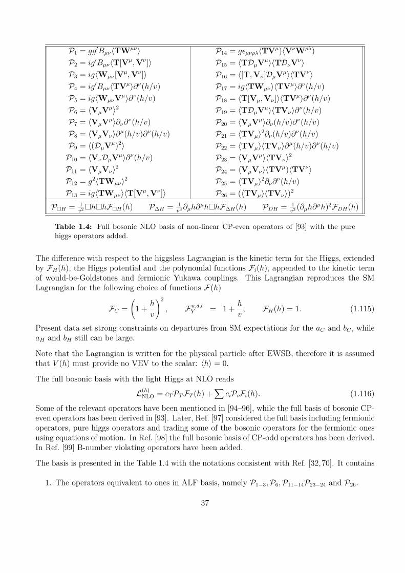
P1 = ggÕBµ‹ÈTWµ‹ÍP2 = igÕBµ‹ÈT[Vµ, V‹ ]ÍP3 = igÈWµ‹ [Vµ, V‹ ]ÍP4 = igÕBµ‹ÈTVµÍˆ‹(h/v)P5 = igÈWµ‹VµÍˆ‹(h/v)P6 = ÈVµVµÍ2

P7 = ÈVµVµÍˆ‹ˆ‹(h/v)P8 = ÈVµV‹Íˆµ(h/v)ˆ‹(h/v)P9 = È(DµVµ)2Í

P10 = ÈV‹DµVµÍˆ‹(h/v)P11 = ÈVµV‹Í2

P12 = g2ÈTWµ‹Í2

P13 = igÈTWµ‹ÍÈT[Vµ, V‹ ]Í

P14 = g‘µ‹fl⁄ÈTVµ)ÈV‹Wfl⁄)P15 = ÈTDµVµÍÈTD‹V‹ÍP16 = È[T, V‹ ]DµVµÍÈTV‹ÍP17 = igÈTWµ‹ÍÈTVµÍˆ‹(h/v)P18 = ÈT[Vµ, V‹ ]ÍÈTVµÍˆ‹(h/v)P19 = ÈTDµVµÍÈTV‹Íˆ‹(h/v)P20 = ÈVµVµÍˆ‹(h/v)ˆ‹(h/v)P21 = ÈTVµÍ2ˆ‹(h/v)ˆ‹(h/v)P22 = ÈTVµÍÈTV‹Íˆµ(h/v)ˆ‹(h/v)P23 = ÈVµVµÍÈTV‹Í2

P24 = ÈVµV‹ÍÈTVµ)ÈTV‹ÍP25 = ÈTVµÍ2ˆ‹ˆ‹(h/v)P26 = (ÈTVµÍÈTV‹Í)2

P⇤H = 1v2⇤h⇤hF⇤H(h) P�H = 1

v3 ˆµhˆµh⇤hF�H(h) PDH = 1v3 (ˆµhˆµh)2FDH(h)

Table 1.4: Full bosonic NLO basis of non-linear CP-even operators of [93] with the purehiggs operators added.

The di�erence with respect to the higgsless Lagrangian is the kinetic term for the Higgs, extendedby FH(h), the Higgs potential and the polynomial functions Fi(h), appended to the kinetic termof would-be-Goldstones and fermionic Yukawa couplings. This Lagrangian reproduces the SMLagrangian for the following choice of functions F(h)

FC =A

1 + h

v

B2

, Fu,d,lY = 1 + h

v, FH(h) = 1. (1.115)

Present data set strong constraints on departures from SM expectations for the aC and bC , whileaH and bH still can be large.

Note that the Lagrangian is written for the physical particle after EWSB, therefore it is assumedthat V (h) must provide no VEV to the scalar: ÈhÍ = 0.

The full bosonic basis with the light Higgs at NLO reads

L(h)NLO = cT PT FT (h) +

ÿciPiFi(h). (1.116)

Some of the relevant operators have been mentioned in [94–96], while the full basis of bosonic CP-even operators has been derived in [93]. Later, Ref. [97] considered the full basis including fermionicoperators, pure higgs operators and trading some of the bosonic operators for the fermionic onesusing equations of motion. In Ref. [98] the full bosonic basis of CP-odd operators has been derived.In Ref. [99] B-number violating operators have been added.

The basis is presented in the Table 1.4 with the notations consistent with Ref. [32,70]. It contains

1. The operators equivalent to ones in ALF basis, namely P1≠3, P6, P11≠14P23≠24 and P26.

37

2. New operators with the derivative acting on the Higgs field, those are P4≠5, P7≠8, P10, P17≠22and P25

3. Operators P9≠10 and P15 have no derivatives on h, but are rewritten in di�erent form incomparison to the usual ALF basis.

4. Pure Higgs operators P⇤H , P�H and PDH .

Counting and renormalization

There is a striking di�erence between the loop structures of the linear and non-linear Lagrangians.Indeed, the LO SMEFT is the SM, it is a renormalizable theory , which in principle can be used tocalculate the observables at any precision, involving as many loop orders as needed. The diagramswith arbitrary number of loops and vertexes belonging to LLin

LO will generate divergent contributionsonly to LLin

LO and therefore LLinNLO is not required for the theoretical consistency. Loops with one

insertion of NLO vertexes will generate only divergences that are to be absorbed by the parametersof LLin

NLO. The insertion of two vertexes from LLinNLO or one from LLin

NNLO will renormalize LLinNNLO

terms and so on. Note that this rule does not depend on the number of loops contained in adiagram.

The situation is not the same for non-linear Lagrangian. Indeed, unless one restricts the parametersof Fi(h) to the SM case, even the LO HEFT Lagrangian is not renormalizable and the countertermsneeded to render the theory finite do not have the structure of LNL

LO . At one loop they willgenerate divergences proportional to the structures of to LNL

NLO as it is demonstrated for examplein original papers [90, 91] and in Chapter 4. Beyond one loop NNLO Lagrangian is required forrenormalization. The non-linear expansion thus is an example of non-decoupling EFT, a theorywhere higher order terms of EFT expansion have to be included to perform renormalization.Strictly speaking the number of counterterms for arbitrary number of loops is infinite. For oneloop though the counterterms needed are the ones presented in Table 1.4.

A more rigorous way to define the order at which a given operator should appear and estimateits coe�cient suppression relies on the use of power counting formula. Naive dimensional analysisformula [58], modified in order to include the weight of the gauge couplings by [100, 101], andapplied for the HEFT case [102] reads

�4

16fi2

Cˆ

�

DNpC

4fi „

�

DN„ 54fi A

�

6NAC

4fi Â

�3/2

DNÂ 5g

4fi

6Ng5

y

4fi

6NyC

⁄

16fi2

DN⁄

. (1.117)

This formula reproduces the correct order 1 coe�cient for the leading order terms, including thecanonically normalized gauge kinetic terms, as well as reveals the suppression of beyond LO terms.

38

Figure 1.6: A representation of the correspondence between SMEFT and HEFT operators.The first order deviations from the SM are highlighted in color [103].

1.3.3 SMEFT vs. HEFT

The correspondence between the two approaches for BSM EFT can be summarised as follows[24,70,82,103–108]

• Higgs couplings. Since in HEFT the Higgs is a singlet under GSM its couplings arecompletely free parameters, while in the SMEFT they are restricted by gauge symmetry,due to the fact that the Higgs belongs to a doublet, and therefore might be correlated to thepure gauge couplings.

• Power counting. SMEFT is organised as an expansion in terms of canonical mass dimen-sion with higher order (d>4) operators suppressed by corresponding powers of the cuto�scale �. In HEFT, with the matrix of Goldstones U being dimensionless, the counting is ac-cording to number of derivatives, similar to the counting of QCD. Moreover Higgs insertionsare are considered all at once as arbitrary functions F(h), with all the powers of Higgs fieldh belonging to the same order of expansion.

• Triple and quartic gauge couplings. Furthermore, triple and quartic gauge and Higgs-gauge couplings are correlated in the SMEFT, while in HEFT they remain decorrelated. Theobservation of such decorrelated couplings would point to the validity of HEFT.

• Couplings strength. Some couplings that are expected to be strongly suppressed in theSMEFT, are instead predicted with higher strength in the HEFT and are potentially visiblein the present LHC run.

The correspondence between SMEFT and HEFT can be identified simply by setting

H = v + hÔ2

UA

01

B

. (1.118)

Each SMEFT operator then corresponds to a combination of sibling operators of HEFT.

39

The two EFTs do not match each other at a given order. Instead, in general the correspondenceconnects operators of di�erent orders in both expansions. This situation is depicted in Fig. 1.6.Moreover, the HEFT expansion contains more free parameters at any given order.

In the Chapter 3 we derive the e�ective non-linear Lagrangian of the linear Goldstone Higgs modeldeveloped before that in Chapter 2. The resulting Lagrangian will contain only a subset of theparameters of the general HEFT.

40

2

The minimal linear sigma model for theGoldstone Higgs

In this chapter we construct a UV complete model of the Goldstone Higgs and study its possibleexperimental validation at LHC as well as possible low energy e�ects. Out of many possible optionsfor the symmetry breaking pattern, we will focus on the minimal case of SO(5)/SO(4) coset. Mostof the literature based on this coset assumes from the start a strong dynamics and uses an e�ectivenon-linear formulation of the model(s) [10,15–21]. This approach has the advantage of being quitegeneral, o�ering a parametrisation of all possible ultraviolet completions for the symmetry groupchosen. At the same time one of its limitations is that it is applicable only in a finite domain ofenergies. Instead, we consider a renormalizable model which in its scalar part is a linear sigmamodel including a new heavy scalar particle ‡, singlet under the gauge group. Our model canbe considered either as an ultimate model made out of elementary fields, or as a renormalizableversion of a deeper dynamics, much as the linear ‡ model is to QCD. One former attempt in thisdirection [22] did not fully take into account and computed the impact of the fermionic sector onthe main phenomenological observables. Later, linearly completed models have been consideredin Refs. [23–26,31,32] and extended the previous analyses.

While the choice of the minimal bosonic sector is clear, there is a number of possible choicesfor the fermionic sector. The option explored in this section assumes heavy fermions in vectorialrepresentations of SO(5), in contrast to models where the SM left doublets are embedded in SO(5)multiplets [22]. Direct couplings between SM fermions and the heavy fermions will be the sourceof the soft SO(5) breaking, while the Higgs particle has tree-level couplings only with the exoticfermionic sector, via SO(5)-invariant Yukawa couplings. It will be discussed how the inducedColeman-Weinberg potential requires soft breaking terms to be included in the scalar potential.

The usual SM Higgs sector is now substituted by a Higgs-‡ sector, correcting the strength of theSM Higgs-gauge boson couplings and opening new interaction channels. The phenomenology ofthe ‡ production and decay will be also studied, including fermionic and bosonic tree-level andone loop decays (e.g. gluon-gluon and photon-photon). Analysis of present Higgs data will beused to set a constraint on the fine-tuning ratio v/f . The contribution of the Higgs, ‡ and theexotic fermions to the oblique S and T parameters will be computed. Particular emphasis will be

41

dedicated to the impact of the ‡ particle on present and future LHC data, produced either viagluon fusion or vector-boson fusion and decaying into a plethora of channels including diphotonfinal state.

Furthermore, we identify some of the leading low-energy bosonic operators stemming from thenew physics when the exotic heavy fermion sector is integrated out. We determine the dominante�ective operators made out of the ‡ field and SM fields, as a first step towards the identificationof a “benchmark” electroweak e�ective Lagrangian, considered in Chapter 3.

2.1 The SO(5)/SO(4) scalar sector

The complete Lagrangian can be written as the sum of three terms describing respectively thepure gauge, scalar and fermionic sectors,

L = Lg + Ls + Lf , (2.1)

where Lgauge reduces to the SM gauge kinetic terms. This section discusses in detail the scalarsector and its interactions, while the study of the fermionic sector is deferred to the next section.

In order to define the linear ‡ model corresponding to an SO(5) symmetry spontaneously brokento SO(4), let us consider a real scalar field „ in the fundamental representation of SO(5). Threeamong its five components will be ultimately associated with the longitudinal components of theSM gauge bosons „i, i = 1, 2, 3, while the other two will correspond to the Higgs particle h andto an additional scalar ‡, respectively. For simplicity the results will be often presented in theunitary gauge (u.g.), in which „i = 0:

„ = („1, „2, „3, h, ‡)T u.g.æ (0, 0, 0, h, ‡)T . (2.2)

The scalar Lagrangian describing the scalar-gauge and the scalar-scalar interactions reads

Ls = 12(Dµ„)T (Dµ„) ≠ V („) , (2.3)

where the SU(2)L ◊ U(1)Y covariant derivative is given by

Dµ„ =1ˆµ + ig�i

LW iµ + igÕ�3

RBµ

2„ (2.4)

and �iL and �i

R as before are the generators of the SU(2)L and SU(2)R subgroups of the custodialSO(4) group contained in SO(5). The embedding of the gauge group SU(2)L ◊ U(1)Y insideSO(5), implicitly assumed in Eqs. (2.2-2.4), is purely conventional. As we will see in section 2.1,both h and ‡ acquire a vacuum expectation value (vev), leaving unbroken an SO(4)Õ subgroupwhich is rotated with respect to the group SO(4) ¥ SU(2)L ◊SU(2)R containing SU(2)L ◊U(1)Y .

For later convenience it is pertinent to introduce the complex notation for the scalar field „ in thefundamental representation of SO(5)

„ =1HT , ÊHT , ‡

2T. (2.5)

42

The relation between the real and the complex notation is given by

„ = 1Ô2

1≠i(Hu + Hd) , Hu ≠ Hd , i(Hd ≠ Hu) , Hd + Hu ,

Ô2‡

2T. (2.6)

2.1.1 The scalar potential

The most general SO(4) preserving while SO(5) breaking renormalizable potential depends a priorion ten parameters. Two of them can be reabsorbed via a redefinition of parameters 1, resulting ona Lagrangian dependent on one SO(5) preserving coupling, ⁄, one scale f heralding spontaneousSO(5)/SO(4) breaking, and six SO(5) soft-breaking terms (denoted below –, —, a1,2,3,4). TheLagrangian in the unitary gauge reads:

V (h, ‡) = ⁄1‡2 + h2 ≠ f 2

22+ –f 3 ‡ ≠ f 2— h2 + a1 f ‡h2 + a2 ‡2h2 + a3 f ‡3 + a4 h4 . (2.7)

In order to retrieve the formulae in a general gauge it su�ces to replace h2 by the SO(4) invariantcombination h2 + „2.

The only strictly necessary soft breaking terms are – and — as they need to be present to absorbdivergences generated by one-loop Coleman-Weinberg contributions to the Lagrangian, as shown inAppendix A; only those terms will be considered in what follows 2, a procedure already previouslyadopted in Ref. [22]. The potential then reads

V (h, ‡) = ⁄1h2 + ‡2 ≠ f 2

22+ –f 3 ‡ ≠ —f 2 h2 , (2.8)

resulting on a system depending on four parameters. The scalar quartic coupling ⁄ can be conven-tionally traded by the ‡ mass, given by m2

‡ ƒ 8⁄f 2 for negligible – and —; the non-linear modelwould be recovered in the limit m‡ ∫ f , that is ⁄ ∫ 1.

A consistent electroweak (EW) symmetry breaking requires both scalars h, ‡ to acquire a non-vanishing vev, respectively dubbed as v and v‡ below, as for v ”= 0 the SO(4) global group andthe EW group are spontaneously broken. Note that the vev of h is identified with the electroweakscale since it can be related to the Fermi constant precisely as in the SM, see Sect. 2.1.2 below.For –, — ”= 0 and assuming v ”= 0, it results

v2‡ = f 2 –2

4—2 , v2 = f 2A

1 ≠ –2

4—2 + —

2⁄

B

, (2.9)

satisfying the conditionv2 + v2

‡ = f 2 (1 + —/2⁄) , (2.10)1Here we choose to get rid of the ‡2 and ‡4 terms.2Full renormalizability of the theory requires, in general, the presence of all gauge invariant operators of dimension

equal to or smaller than four. At two or more loops, the renormalization procedure may thus require to includefurther symmetry breaking terms beyond those considered; we will assume that their finite contributions will beweighted by comparatively negligible coe�cients and can be safely omitted in our analysys.

43

which indicates that the SO(5) vev is “renormalized” by the — term in the potential. FromEqs. (2.9) and (2.10) it follows that both f 2 > 0 and f 2 < 0 are in principle allowed 3, in appropriateregions of the parameters (–, —, ⁄). However, in the SO(5)-invariant limit, for negative f 2 theminimum of the potential is at the origin and in consequence the symmetry is unbroken and thereare no Goldstone bosons. The focus of this section is instead set on the interpretation of the Higgsparticle as a PNGB, which requires f 2 > 0 as well as |v| < |v‡|, the latter condition defining theregion in parameter space continuously connected with the limiting case v = 0 in which the Higgsparticle becomes a true Goldstone boson. For f 2 > 0, the positivity of v2 in Eq. (2.9) and the|v| < |v‡| constraint lead respectively to the conditions 4

–2 < 4—2A

1 + —

2⁄

B

, (2.11)

2—2A

1 + —

2⁄

B

< –2 , (2.12)

which for |—| π ⁄ would indicate 2—2 . –2 . 4—2. Moreover, in order to get v2 π f 2, Eq. (2.9)requires a fine-tuning such that –/2— is very close to unity.

Expanding the ‡ and h fields around their minima, h © h + v and ‡ © ‡ + v‡, and diagonalizingthe scalar mass matrix, the mass eigenstates are given by

hphys = h cos “ ≠ ‡ sin “ , ‡phys = ‡ cos “ + h sin “ . (2.13)

For simplicity, from now on the notation hphys and ‡phys will be traded by h and ‡, respectively.The mixing angle in Eq. (2.13) is given by

tan 2“ = 4vv‡

3v2‡ ≠ v2 ≠ f 2 (2.14)

and should remain in the interval “ œ [≠fi/4, fi/4] in order not to interchange the roles of theheavy and light mass eigenstates. The mass eigenvalues are given by

m2heavy, light = 4⁄f 2

Y]

[

A

1 + 34

—

⁄

B

±C

1 + —

2⁄

A

1 + –2

2—2 + —

8⁄

BD1/2Z^

\ , (2.15)

where the plus sign refers to the heavier eigenstate. For f 2 > 0, the squared masses are positive ifthe following two conditions are satisfied 5

3— + 4⁄ > 0 , 2—2 + 4—⁄ ≠ –2⁄/— > 0 , (2.16)

with the second constraint coinciding with that in Eq. (2.11) multiplying it by 1/(4—⁄); it followsthat — > 0. If the soft mass term proportional to — in the scalar potential Eq. (2.8) would beoverall positive (as for instance for f 2<0 and — > 0), the minimum would always correspond to

3For f2 < 0, – would have to be purely imaginary because of hermiticity.4For f2 < 0, the inequality Eq. (2.11) is reverted.5For f2 < 0, both inequalities in Eq. (2.16) are reverted and as a consequence — < 0.

44

an undesired symmetric EW vacuum v = 0. Assuming the SO(5) explicit breaking to be small,|—|/4⁄ π 1 which may only happen for positive f 2, the masses of the heavy and light eigenstatesread

m2heavy

= 8⁄f 2 + 2—(3f 2 ≠ v2) + O

A—

4⁄

B

,

m2light

= 2—v2 + O

A—

4⁄

B

.

(2.17)

The physical scalars thus correspond to a “light” state with mass O(Ô

—v) and a “heavy” state withmass O(

Ô⁄f). It will be later shown that, for a PNGB Higgs particle (that is v < v‡ and f 2 > 0),

the less fine-tuned regions in parameter space correspond to the case mlight = mh and mheavy = m‡

in the equations above. In fact, would the ‡ particle be lighter than the Higgs, the roles of thelighter and heavier eigenstates would be flipped and the mixing angle “ will be necessarily outsidethe region quoted above. The lighter ‡ scenario is quite di�erent from the typical Higgs PNGBscenarios considered in the literature.

Notice that for mh < m‡ and at variance with the SM case, in the regime of small soft SO(5)breaking the mass of the Higgs and its quartic self-coupling are controlled by two di�erent param-eters, — and ⁄, respectively. This is consistent with the PNGB nature of the Higgs boson whosemass should now appear protected from growing in the strong interacting regime of the theory–corresponding to large ⁄– in which instead the ‡ mass would increase. In other words, we havereplaced the hierarchy problem for the Higgs particle mass by a sensitivity of the ‡ particle toheavier scales: the ‡ mass represents generically the heavy UV completion. The expression for mh

shows that the value of the — parameter for small —/4⁄ is expected to be — ≥ m2h/2v2 ≥ 0.13.

2.1.2 Scalar-gauge boson couplings

In the unitary gauge, the kinetic scalar Lagrangian written in terms or the unrotated fields reads

Ls,kin = 12(ˆµ‡)2 + 1

2(ˆµh)2 + g2

41h + v

22W +

µ W µ≠ + (g2 + gÕ2)8

1h + v

22ZµZµ ,

and justifies the previous identification of the Higgs vev v with the electroweak scale defined fromthe W mass.

The rotation to the physical h, ‡ fields results in the following Lagrangian for the scalar andscalar-gauge interactions, for mh < m‡,

Ls = 12(ˆµ‡)2 + 1

2(ˆµh)2 ≠ 12m2

‡‡2 ≠ 12m2

hh2 ≠ ⁄1h2 + 2 h ‡ + ‡2

22≠

≠ 4⁄(v cos “ ≠ v‡ sin “)1h3 + h ‡2

2≠ 4⁄(v sin “ + v‡ cos “)

1‡3 + h2 ‡

2+

+ (1 + h

vcos “ + ‡

vsin “)2

3M2

W W +µ W µ≠ + 1

2M2ZZµZµ

4. (2.18)

The physical Higgs couplings are thus seen to be weighted down by a cos “ factor with respect tothe SM Higgs ones, while the ‡ field acquires the same interactions than h albeit weighted down

45

by sin “, a fact rich in phenomenological consequences to be discussed further below. The SM limitis recovered when the ‡ field is decoupled from the spectrum and cos “ = 1 follows from Eqs. (2.9)and (2.14). Conversely, for mh > m‡ the mixing dependence would correspond to the interchangecos “ ¡ sin “ in Eq. (2.18).

2.1.3 Renormalization and scalar tree-level decays

The four independent parameters of the scalar Lagrangian can be expressed in terms of fourobservables, which we choose to be:

GF © (Ô

2v2)≠1, mh, m‡, sin “ , (2.19)

with the Fermi constant GF as measured from muon decay and mh from the Higgs pole mass, whilem‡ could be determined from future measurements of the ‡ mass, and sin “ from either deviationsof the Higgs couplings or from the ‡ line shape obtained from its decay into four leptons form‡ Ø 300 GeV, analogous to the case of a heavy SM Higgs boson 6.

Using Eqs. (2.9), (2.14), and (2.15), the exact expressions for the h and ‡ vevs in terms of thosephysical parameters can be obtained

v =1Ô

2GF

2≠1/2,

v‡ = v sin(2“)(m2‡ ≠ m2

h)m2

‡ + m2h ≠ (m2

‡ ≠ m2h) cos(2“) .

(2.20)

These expressions in turn allow to express in terms of measured quantities the four independentparameters of the scalar potential Eq. (2.8), which can be written as

⁄ = sin2 “m2‡

8v2

A

1 + cot2 “m2

h

m2‡

B

,

—

4⁄= m2

hm2‡

sin2 “m4‡ + cos2 “m4

h ≠ 2m2hm2

‡

,

–2

4—2 = sin2(2“)(m2‡ ≠ m2

h)2

4(sin2 “m4‡ + cos2 “m4

h ≠ 2m2hm2

‡) ,

f 2 = v2(sin2 “m4‡ + cos2 “m4

h ≠ 2m2hm2

‡)(sin2 “m2

‡ + cos2 “m2h)2 .

(2.21)

The above exact formulae show that the mixing angle “ does not coincide with the parameterÔ

›,except in the limit m‡ ∫ mh (or more precisely —/4⁄ π 1 and v2 π f 2), where for sizeable sin “

6For a lighter ‡, the decay width becomes too narrow –possibly even below the experimental resolution– andmore ingenious procedures would be required to determine the scalar mixing strength, such as for instance on-shellto o�-shell cross section measurements [109].

46

10-3 10-2 10-1 100 1010.0

0.2

0.4

0.6

0.8

1.0

ms HTeVL

sin2 g

noPNGB

h=PNGB

s=PNGB f 2 < 0

bêl=0.3

bêl=0.01

aêb = 1

aêb=2

Figure 2.1: m‡ versus sin2 “ parameter space of the scalar sector. The Higgs mass mh andthe Higgs vev v have been fixed to their physical values. The red region corresponds to f2 < 0,for which the SO(5)-invariant part of the potential is unbroken and there are no Goldstonebosons in the symmetric limit. The region where |v| > |v‡| is shown in brown (these regionsare excluded by Higgs data, see text). The Higgs is a pseudo-Goldstone boson within thewhite regions at the bottom-right and the top-left part of the plane.

the last equation above leads to

sin2 “ ≠æm‡/mh∫1

v2

f 2 + 4m2h

m2‡

. (2.22)

A few comments regarding the parameter space and the scalar spectrum are in order, as arbitraryvalues of m‡ and sin2 “ are not allowed if we insist on interpreting the Higgs boson as the pseu-dogoldstone boson of a spontaneous SO(5) breaking. Fig. 2.1 displays the (m‡, sin2 “) plane: ateach point the scalar sector is completely defined as mh and v are fixed to their physical values.The di�erently colored regions correspond to

• No SO(5) breaking in the light red region, where f 2 < 0; its red borders depict the f 2 = 0frontier;

• The ‡ particle being the PNGB of the spontaneous breaking of SO(5) in the light brownregion, where v‡ < v;

• The Higgs as the PNGB of the SO(5) æ SO(4) breaking in the white areas, where v < v‡

and the Higgs would became a true goldstone boson in the absence of EW breaking (v æ 0).

47

A complementary divide is provided by the value of the Higgs mass:

• On the mh < m‡ region to the right of the figure, the physical Higgs couplings to SM particlesare weighted down by cos “ with respect to SM values, see for instance Eq. (2.18). It will beshown in the next sections that present LHC Higgs data only allow for values sin2 “ < 0.18at 2‡ CL, though, leaving as allowed parameter space a fraction of the lower white (HiggsPNGB) section of the figure. The analysis in the next sections will thus focus in this regime,for which Fig. 2.1 already suggests a lower bound on m‡ of a few hundreds of GeV. Therelative importance of the soft breaking terms is also illustrated through the curves depictedfor fixed –/— and —/⁄;

• On the m‡ < mh area to the right of the figure, the physical Higgs couplings to SM particlesare instead weighted down by sin “, whose value will thus be bounded by sin2 “ > 0.82 at2‡ CL. It thus remains as available zone the upper part of the upper white (Higgs PNGB)region. Nevertheless, the quartic coupling ⁄ is there very small, typically ⁄ < 10≠3, makingthe SO(5) invariant potential very flat and potentially unstable against radiative corrections;furthermore, if the soft breaking parameters are required to be small compared to the sym-metric term, –, — < ⁄, their values may require extra fine-tuning with respect to radiativecorrections from the fermionic sector to be discussed further below. For these reasons we willnot dwell further below on the case m‡ < mh even if phenomenologically of some interest.

Extending the renormalization scheme to the gauge sector, we choose the two extra observablesneeded to be the mass of the Z boson and the fine structure constant,

MZ , –em = e2

4fi, (2.23)

with MZ and –em as determined from Z-pole mass measurements and from Thompson scattering,respectively [110]. In our model, the relation between the gauge boson masses is the same thanthat for the SM,

MW = cos ◊W MZ , (2.24)where the weak angle is given at tree-level by

sin2 ◊W = 12

A

1 ≠Û

1 ≠ 4fi–emÔ2GF M2

Z

B

. (2.25)

Using all the above, it is straightforward to compute the relevant tree-level branching ratios forthe heavy and light scalar boson decays into SM bosons:

�(h æ WW ú) = �SM(h æ WW ú) cos2 “ ,

�(h æ ZZú) = �SM(h æ ZZú) cos2 “ ,

�(‡ æ W +W ≠) =Ô

2GF

16fim3

‡ sin2“

C

1 + OA

M2W

m2‡

B D

,

�(‡ æ ZZ) =Ô

2GF

32fim3

‡ sin2“

C

1 + OA

M2Z

m2‡

BD

,

48

�(‡ æ h h) =Ô

2GF

32fim3

‡ sin2“

C

1 + OA

m2h

m2‡

BD

, (2.26)

where the SM widths can be found for instance in Ref. [111]. The ‡ partial widths above willdominate the total ‡ width unless the mixing is unnaturally tiny, and thus measuring the branchingratios is not enough to infer the value of the scalar mixing. It is easy to see that

�‡

m‡ƒ m2

‡ sin2 “

8v2 , (2.27)

and thus the measurement of the line shape of the ‡ seems feasible only for m‡ above the EWbreaking scale (assuming non-negligible mixing). In that regime, the value of sin “ can be inferredfrom the line shape and all other observables in Eq. (2.26) can then be predicted in terms of thephysical parameters defining our renormalization scheme. Other bosonic decay channels requiringone-loop amplitudes will be discussed later on.

2.2 Fermionic sector

The fermionic sector is unavoidably an important source of model dependency as diverse choicesof SO(5) fermionic multiplets are possible. Moreover the achievement of the desired symmetrybreaking pattern in “composite Higgs” models relies on the fermionic sector. A schematic pictureis given in Fig. (2.2) considering a high energy global symmetry group - SO(5) in the case underdiscussion:

• Heavy scalar and fermion representations of the high-energy global symmetry are considered.SO(5) breaks spontaneously to SO(4) at a scale f , resulting in four massless Goldstonebosons: the three longitudinal components of the electroweak gauge bosons and a “HiggsGoldstone boson”. The fifth component ‡ remains massive.

• Furthermore, SO(5) is explicitly broken by the coupling of the exotic heavy representationsto the SM fermions (soft breaking) and to the gauge bosons (hard breaking). This inducesat one-loop a potential for the h field with a non-trivial minimum, providing a mass for hand breaking the SM electroweak symmetry at a scale v ”= f .

Several “minimal” possibilities have been explored in the literature for the exotic fermionic repre-sentations (see for instance Refs. [16, 22]). The setup considered here contains:

1. Heavy (exotic) vector-like fermions in complete representations of SO(5), either in the fun-damental representation, denoted below by Â - or singlets denoted by ‰.

2. A scalar field „ in the fundamental representation of SO(5), which contains the h and ‡particles. Its vev breaks SO(5) spontaneously to SO(4)Õ. By construction only the heavyexotic fermions couple directly to the scalar „.

49

Figure 2.2: Schematics of the SO(5) æ SO(4) model

Figure 2.3: Schematics of light fermion mass generation. The light SM fermions -here thetop quark- couple to the heavy partners breaking explicitly SO(5). The middle image depictsthe SO(5) invariant Yukawa interactions between the Higgs and the heavy partners. Thecombination of both couplings induces and e�ective top Yukawa coupling and thus a massivetop quark.

3. The Higgs field couples to the exotic fermions only via SO(5) invariant Yukawa couplings.The sources of SO(5) breaking lie instead in the electroweak gauge interactions and in mixingterms between the heavy exotic fermions and the SM fermions. Such a breaking is fed vialoop corrections to the scalar potential, where it is modeled by two SO(5) soft breakingterms which are custodial preserving.

This choice of fermionic representation respects an approximate custodial symmetry which protectsthe Zbb coupling [112]. Fig. (2.3) illustrates a characteristic of the partially composite fermionicsector in this class of models [29]: a seesaw-like mechanism is at work in the generation of alllow-energy fermion masses. The heavier the exotic fermions the lighter the light fermions.

To ensure correct hypercharge assignments for the SM fermions coupled directly to heavy exoticfields, the global symmetry is customarily enlarged by (at least) an extra U(1)X sector, leadingfinally to a pattern of spontaneous global symmetry breaking given by

SO(5) ◊ U(1)X æ SO(4) ◊ U(1)X ¥ SU(2)L ◊ SU(2)R ◊ U(1)X , (2.28)

with the hypercharge corresponding now to a combination of the new generator and that of SU(2)R

50

generator, see Eq. (2.4),

Y = �(3)R + X . (2.29)

As the global U(1)X symmetry remains unbroken, no additional Goldstone bosons are generated.Two di�erent U(1)X charges are compatible with SM hypercharge assignments: 2/3 and ≠1/3. Wewill indeed consider two di�erent copies of heavy fermions for each representation, di�erentiatedby the U(1)X , as they are necessary to induce mass terms for both the SM up and the down quarksectors. Schematically, the fundamental and singlet representations can be decomposed underSU(2)L quantum numbers as follows,

Â(2/3) ≥ (X, Q, T (5)) , Â(≠1/3) ≥ (QÕ, X Õ, B(5)) ,

‰(2/3) ≥ T (1) , ‰(≠1/3) ≥ B(1) ,

where X(Õ), Q(Õ) denote the two di�erent SU(2)L doublets contained in the fundamental represen-tation of SO(5). In each multiplet, the first doublet has �(3)

R = 1/2 while the second one has�(3)

R = ≠1/2. T(1,5), B(1,5) denote instead SU(2)L ◊ SU(2)R singlets, respectively in the 5 and1 representation of SO(5). Table 2.1 summarizes the relevant quantum numbers for all heavyfermions.

Charge/Field X Q T(1,5) QÕ X Õ B(1,5)

�(3)R +1/2 ≠1/2 0 +1/2 ≠1/2 0

SU(2)L ◊ U(1)Y (2, +7/6) (2, +1/6) (1, +2/3) (2, +1/6) (2, ≠5/6) (1, ≠1/3)

x +2/3 +2/3 +2/3 ≠1/3 ≠1/3 ≠1/3

qEM

Xu = +5/3

Xd = +2/3

Qu = +2/3

Qd = ≠1/3+2/3

QÕu = +2/3

QÕd = ≠1/3

X Õu = ≠1/3

X Õd = ≠4/3≠1/3

Table 2.1: Heavy fermion charges assignments.

The fermionic Lagrangian

For the SM fermions, the analysis below will be restricted to the third generation of SM quarksfor simplicity, denoting by qL and tR and bR the doublet and singlets, respectively. It would bestraightforward to extend the results to the other two generations, for instance introducing heavierreplica of the exotic sector, leading to very minor additional phenomenological impact.

Assuming the “minimal” content specified in the previous sections, the fermionic Lagrangian isgiven by

LF = qLi /DqL + tRi /DtR + bRi /DbR

+ Â(2/3)1i /D ≠ M5

2Â(2/3) + Â(≠1/3)

1i /D ≠ M Õ

5

2Â(≠1/3)

+ ‰(2/3)1i /D ≠ M1

2‰(2/3) + ‰(≠1/3)

1i /D ≠ M Õ

1

2‰(≠1/3)

51

≠5

y1 Â(2/3)L „ ‰(2/3)

R + y2 Â(2/3)R „ ‰(2/3)

L + yÕ1 Â(≠1/3)

L „ ‰(≠1/3)R + yÕ

2 Â(≠1/3)R „ ‰(≠1/3)

L

+ �11qL�(2/3)

2◊5

2Â(2/3)

R + �2 Â(2/3)L

1�(2/3)

5◊1 tR

2+ �3 ‰(2/3)

L tR

+ �Õ1

1qL�(≠1/3)

2◊5

2Â(≠1/3)

R + �Õ2 Â(≠1/3)

L

1�(≠1/3)

5◊1 bR

2+ �Õ

3 ‰(≠1/3)L bR + h.c.

6. (2.30)

The first lines contain the kinetic terms for the SM fermions. The second and third lines includethe kinetic and mass terms for the exotic fermions. The kinetic terms become SO(5)-invariantin the gaugeless limit. The fourth line contains the SO(5) invariant Yukawa couplings of theexotic sector to the Higgs field. Finally, the last two lines of the Lagrangian contain the SO(5)soft-breaking interactions of SM fermions with exotic fermions. �2◊5 and �5◊1 denote suitablespurions connecting SO(5) and SU(2) ◊ U(1) representations. If the primed parameters were setto zero no bottom mass would be generated through this mechanism. All parameters in Eq. (2.30)are assumed real for simplicity, that is, we will assume CP invariance in what follows.

It is useful to rewrite the Lagrangian in Eq.(2.30) in terms of SU(2)L components. For thispurpose, from this point and until Eq. (2.39) below, h and ‡ will denote again the unshifted andunrotated original scalar fields in Eq. (2.8):

LF = qLi /DqL + tRi /DtR + bRi /DbR + Q1i /D ≠ M5

2Q + X

1i /D ≠ M5

2X

+ T (5)1i /D ≠ M5

2T (5) + T (1)

1i /D ≠ M1

2T (1) + QÕ

1i /D ≠ M Õ

5

2QÕ + X Õ

1i /D ≠ M Õ

5

2X Õ

+ B(5)1i /D ≠ M Õ

5

2B(5) + B(1)

1i /D ≠ M Õ

1

2B(1)

≠5

y11XLHT (1)

R + QLÊHT (1)

R + T (5)L ‡T (1)

R

2+ y2

1T (1)

L H†XR + T (1)L

ÊH†QR + T (1)L ‡T (5)

R

2

+ yÕ1

1X Õ

LÊHB(1)

R + QÕLHB(1)

R + B(5)L ‡B(1)

R

2+ yÕ

2

1B(1)

LÊH†X Õ

R + B(1)L H†QÕ

R + B(1)L ‡B(5)

R

2

+ �1qLQR + �Õ1qLQÕ

R + �2T(5)L tR + �3T

(1)L tR + �Õ

2B(5)L bR + �Õ

3B(1)L bR + h.c.

6. (2.31)

Eq. (2.31) shows that the light fermion masses must be proportional to the SO(5) invariant Yukawacouplings of heavy fermions and to the explicitly SO(5) breaking light-heavy fermionic interactions.The generation of light quark masses requires a vev for the scalar doublet H. For instance, a tLtR

mass term is seen to result from the following chain of couplings,

ql ≠æ�1

QR ≠æM5

QL ≠æy1ÈHÍ

T (1)R ≠æ

M1T (1)

L ≠æ�3

tR , (2.32)

suggestingmt Ã y1

�1 �3

M1 M5v , (2.33)

see also Fig. 2.3 and Sect. 2.5. Furthermore, both the +2/3 and ≠1/3 electrically charged sectorsacquire o�-diagonal mixing terms.

The expression for the fermionic Lagrangian Eq. (2.31) can be rewritten in a compact formdefining a fermionic vector whose components are ordered by their electrical charges qEM =(+5/3, +2/3, ≠1/3, ≠4/3),

� =1Xu, T , B, X Õd

2, (2.34)

52

where T and B include the top and bottom quarks together with their heavy fermionic partners

T =1t, Qu, Xd, T (5), T (1), QÕu

2, B =

1b, QÕd, X Õu, B(5), B(1), Qd

2. (2.35)

The fermion mass terms in the weak basis can then be written as

LM = ≠�L M(h, ‡) �R, (2.36)

where here and in what follows the sum over all components of the fermionic vector is left implicitand the block diagonal 14 ◊ 14 fermion mass matrix M reads

M(h, ‡) = diag1M5, MT (h, ‡), MB(h, ‡), M Õ

5

2, (2.37)

MT (h, ‡) =

Q

cccccccca

R

ddddddddb

0 �1 0 0 0 �Õ1

0 M5 0 0 y1hÔ2 0

0 0 M5 0 y1hÔ2 0

�2 0 0 M5 y1‡ 0�3 y2

hÔ2 y2

hÔ2 y2‡ M1 0

0 0 0 0 0 M Õ5

, (2.38)

MB(h, ‡) = MT (h, ‡) with {yi, �i, Mi} ¡ {yÕi, �Õ

i, M Õi} . (2.39)

The mass matrices can be diagonalised by bi-unitary (or for the case of the real parameters bi-orthogonal) transformations,

�physL = L�L , �phys

R = R�R , Mdiag = L†MR . (2.40)

These matrices can be diagonalized analytically in some interesting limits; in general they will bediagonalized numerically.

The physical light eigenstates are admixtures of the light and heavy fermion fields appearing inthe Lagrangian. The scalar fields vevs induce in addition heavy fermion mass splittings. Noticehowever that, even in the limit of vanishing Yukava couplings, the exotic fermions get mixed viathe SO(5) breaking couplings. Moreover, although the various dimensional couplings �i and �Õ

i

in Eqs. (2.30) and (2.31) may be of the same order, the top and bottom components of the heavydoublets are splitted by SO(4) breaking terms, generically of O(yiv).

2.3 Phenomenology

In this section, bounds are derived first on the model parameters resulting from present LHC Higgsdata and from electroweak precision tests - namely S,T and gb

L. Future signals are discussed next,focusing in particular on ‡ physics.

53

2.3.1 Bounds from Higgs measurements

The tree-level mixing of the scalar singlet ‡ with the Higgs resonance h can be strongly boundedfrom present data and in particular from h to ZZ and W +W ≠ decays, and from h-gluon-gluontransitions: the Higgs coupling strength to SM fields is weighted down simply by a cos “ factor withrespect the SM value, as previously explained and shown in Eq. (2.18). We use ATLAS and CMScombined results for the gluon-gluon and vector boson mediated Higgs production processes [113].

A ‰2 fit taking into account the correlation between the corresponding coupling modifiers in thecombined fit of the 7 and 8 TeV LHC data -given by figure 23.B of Ref. [113]- constrains directlycos “, translating into the following bound

sin2 “ . 0.18 (at 2‡) , (2.41)

which in the m‡ ∫ mh limit would point to a value for the non-linearity parameter of compositeHiggs models, › © v2/f 2 ≥ sin2 “, consistent with the limits found in the literature [69], seeEqs. (2.21) and (2.22) and the discussion below.

Comparison with literature on non-linear realizations

Ref. [69] shows that in non-linear realizations of the composite Higgs scenario the behaviour of theHiggs couplings modifications varies depending on the SO(5) fermionic representations chosen. Inparticular they compare the so called MCHM4 and MCHM5 scenarios:

• In MCHM4, the fermions (both the embedded light ones and the heavy partners) are in the 4(spinorial) representation of SO(5); the coupling modifiers then obey Ÿ(4)

V = Ÿ(4)f = (1≠›)1/2,

leading to a bound from Higgs data ›(4) < 0.18 at 2‡ CL. MCHM4 is actually ruled out byits impact on the Zbb coupling and thus for instance disregarded in Ref. [16].

• In MCHM5, the fermions are instead in the 5 (fundamental) of SO(5), and in this caseŸ(5)

V = (1 ≠ ›)1/2 di�ers from Ÿ(5)f = (1 ≠ 2›)(1 ≠ ›)≠1/2, that is, Ÿ(5)

f /Ÿ(5)V ¥ 1 ≠ › for small ›

values. LHC Higgs data set then a bound ›(5) < 0.12 at 2‡ CL.

Now, the heavy fermion configuration of our model seems alike to that in MCHM5 if the ‡ particlewas disregarded (‡ does not intervene in the tree-level Higgs data analysis of SM couplings),and in spite of including one heavy fermion in a 1 (singlet) of SO(5) as the latter could beintegrated out to mimic the MCHM5 spectrum discussed for instance in Refs. [114] or [16].Indeed, according to the notation in Ref. [16], the fermion representation in our model would begiven by MCHMQ≠T ≠B æ MCHM5≠5,1≠5,1; nevertheless, the behaviour for the modifiers –andthus the resulting › bound– is the same than in MCHM4, see Eq. (2.41). Plausibly, this apparentparadox may be resolved by taking into account that the limit of very heavy ‡ corresponds tothe ⁄ coupling reaching the non-perturbative regime, and a resumation of the strong interactinge�ects may be needed to fully reach the non-linear regime.

54

2.3.2 Precision electroweak constraints

Analyses available on precision tests for composite Higgs models, such as that in Ref. [115], tend toconsider non-linear versions of the theory where the only scalar present is the Higgs particle, butfor Ref. [22], which discusses qualitatively the interplay of scalar and exotic fermion contributions.see also Ref. [12]. We present here an explicit computation of the scalar (h and ‡) and exoticfermion contributions, discussing the impact of varying the ‡ mass. S, T and U parameters areconsidered together with gb

L and parameter correlations.

S, T and gbL

Consider the parameter definitions in Ref. Ata ,

– S = 4sW cWd�30(q2)

dq2 |q2=0 = 4sW cW F30 ,

– T = 1M2

W

[�11(0) ≠ �33(0)] = 1M2

W

[A11 ≠ A33] ,

– U = ≠4s2W

d

dq2 [�33(q2) ≠ �11(q2)]|q2=0 = 4s2W (F11 ≠ F33) , (2.42)

where cW (sW ) denotes the cosinus (sinus) of the Weinberg angle cW = MW /MZ , and the elec-troweak vacuum polarization functions are given by

�µ‹ij (q) = ≠i[�ij(q2)gµ‹ + (qµq‹ ≠ terms)] ; �ij(q2) © Aij(0) + q2Fij + ... (2.43)

with i, j = W, Z or i, j = 0, 3 for the B or the W3 bosons, respectively, and the dots indicatingan expansion in powers of q2. We will not consider further U as it typically corresponds to higherorder (mass dimension eight) couplings while only low-energy data (e.g. LEP) will be used here 7.On the contrary, relevant constraints could stem from deviations induced in the ZbLbL coupling,parametrised by gb

L in the decay amplitude

MZæbLbL= ≠ e gb

L

sW cWb(p2) /‘(q)1 ≠ “5

2 b(p1), (2.44)

where ‘(q) denotes the Z boson polarization and pi the b quark and antiquark momenta.

The values of S, T and gbL are allowed to deviate from the SM prediction within the constraints [115,

117]�S © S ≠ SSM = 0.0079 ± 0.095 ,

�T © T ≠ TSM = 0.084 ± 0.062 ,

�gbL © gb

L ≠ gbLSM = (≠0.13 ± 0.61) ◊ 10≠3 , (2.45)

with the (S, T, gbL) correlation matrix given by

Q

ca1 0.864 0.06

0.864 1 0.1230.06 0.123 1

R

db . (2.46)

7Some other handful parameter definitions are: ‘1 © –T ; ‘3 = –S /(4s2W ), see Ref. [116].

55

Scalar contributions in the linear SO(5) model: h and ‡

Given the scalar couplings in Eq. (2.18), their contributions to S and T can be formulated as

�T (h and ‡) = ≠�T hSM(mh) + c2

“�T hSM(mh) + �T (‡) = s2

“

Ë≠�T h

SM(mh) + �T hSM(m‡)

È, (2.47)

�S(h and ‡) = ≠�ShSM(mh) + c2

“�ShSM(mh) + �S(‡) = s2

“

Ë≠�Sh

SM(mh) + �ShSM(m‡)

È, (2.48)

where the ‡ contributions �T (‡) and �S(‡) have been simply written in terms of the usual SMformulae for the Higgs contribution �T h

SM and �ShSM with the replacement mh æ m‡ and using

the formulae valid for masses much above the electroweak scale. The scalar contribution to �T isthen given by

�T (h and ‡) =3GF M2W

8fi2Ô

2s2

“

Q

a ≠ m2h

log(m2h/M2

W )M2

W ≠ m2h

+ m2‡

log(m2‡/M2

W )M2

W ≠ m2‡

+ M2Z

M2W

I

m2h

log(m2h/M2

Z)M2

Z ≠ m2h

≠ m2‡

log(m2‡/M2

Z)M2

Z ≠ m2‡

J R

b ,

(2.49)

which in the limit m‡ ∫ mh, MW , MZ reduces to

�T (h and ‡) ≥ s2“

3GF M2W

8fi2Ô

2s2

W

c2W

log(m2‡/M2

W ) . (2.50)

For the �S corrections, the formulation in Refs. [118,119] is used, leading to

–�ShSM(m) = s2

W

2GFÔ2fi2

M2W

Q

a x

12(x ≠ 1) log(x) +A

≠x

6 + x2

12

B

F (x) ≠A

1 ≠ x

3 + x2

12

B

F Õ(x)R

b ,

(2.51)

where x © m2/M2Z and for x < 4:

F (x) = 1 +3

x

x ≠ 1 ≠ 12x

4log x ≠ x

Û4x

≠ 1 arctanÛ

4x

≠ 1 ,

F Õ(x) = ≠1 + x ≠ 12 log x + (3 ≠ x)

Ûx

4 ≠ xarctan

Û4x

≠ 1 ,

(2.52)

while for x > 4:

F (x) = 1 +3

x

x ≠ 1 ≠ 12x

4log x ≠ x

Û

1 ≠ 4x

log3Ú

x

4 ≠ 1 +Ú

x

4

4,

F Õ(x) = ≠1 + x ≠ 12 log x + (3 ≠ x)

Ûx

x ≠ 4 log3Ú

x

4 ≠ 1 +Ú

x

4

4.

(2.53)

In the limit of very large m‡, the ‡ contribution to S can be approximated by:

– �S(‡) ≠æ‡æŒ

s2“s2

W

2GFÔ2fi2

M2W

C112 log

Am2

‡

M2W

BD

, (2.54)

56

-0.05 0.00 0.05 0.10 0.15 0.20-0.10

-0.05

0.00

0.05

0.10

DS

DT

‡Ê

f = 1 TeV‡ ms = 2 TeV, sg2 = 0.04Ê ms = 6 TeV, sg2 = 0.06

Figure 2.4: Uncombined contributions of the scalar sector (black curve) and the exoticfermionic sector to the parameters S and T .

consistent with the statements in the literature for a very heavy Higgs particle [65].

The black curve in Fig. 2.4 displays examples of the �S and �T corrections induced by the ‡scalar as it follows from the formulae shown above. As earlier explained, the set of parameters inthe scalar potential (f , ⁄ , – , —) has been traded by four observables: GF , mh, m‡ and the scalarmixing “ (with the latter two yet to be experimentally measured). It is nevertheless theoreticallyilluminating to indicate the corresponding values for f and the scalar quartic self-coupling ⁄ foreach example analyzed, and their values are shown in all figures to follow. We present numericalresults for two typical parameter regimes:

• m‡ = 2 TeV, s2“ = 0.04, which corresponds to f = 1 TeV and to scalar potential couplings

⁄ = 0.38, – = 0.35 and — = 0.16, which clearly lie within the perturbative regime of thelinear SO(5) sigma model.

• m‡ = 6 TeV, s2“ = 0.06, which also correspond to f = 1 TeV, while ⁄ = 4.3 -closer to the limit

of validity of the perturbative expansion- and – = 0.25, — = 0.13; this pattern correspondsthen to a mainly SO(5) symmetric scenario with small soft symmetry breaking.

Fig. 2.4 shows a sizeable negative contribution of the ‡ particle to �T which increases with m‡,and positive contribution to �S; the result is consistent with the pattern expected in Ref. [22],and similar to that for the heavy Higgs case (see e.g. Ref. [120]). In the limit m‡ æ mh the totalscalar contribution matches that in the SM due to the Higgs particle. It is easy to extrapolate theS and T scalar contributions to other mixing regimes as they scale with s2

“: for instance the e�ectwould be amplified by a factor of ≥ 3 when raising the mixing towards the maximal value allowed,see Eq (2.41).

For gbL instead we will not analyze the one-loop ‡ contributions, as they would be proportional to

the bottom Yukawa couplings and thus negligible compared to the top and top-partner contribu-tions to be discussed next.

57

-0.2 -0.1 0.0 0.1 0.2 0.3 0.4-0.10

-0.05

0.00

0.05

0.10

0.15

0.20

DS

DT

f = 1 TeVonly fermions

-0.2 -0.1 0.0 0.1 0.2 0.3 0.4-0.10

-0.05

0.00

0.05

0.10

0.15

0.20

DS

DT

ms = 2 TeV, sg2 = 0.04

fif = 1 TeV, l = 0.38a = 0.35, b = 0.16

-0.2 -0.1 0.0 0.1 0.2 0.3 0.4-0.10

-0.05

0.00

0.05

0.10

0.15

0.20

DS

DT

ms = 6 TeV, sg2 = 0.06

fif = 1 TeV, l = 4.3a = 0.25, b = 0.13

Figure 2.5: Combined contributions to S and T from the scalar sector and the exoticfermionic sector. The blue, green and red points are allowed at 1, 2, 3‡ by the combined(S, T, gb

L) fit, while gray points are outside the 3‡ region.

Fermionic contributions

The heavy fermion sector may have an impact on the oblique parameters and on gbL. This sector

adds additional parameter dependence on top of the four renormalization parameters alreadydiscussed for the scalar sector of the linear SO(5) sigma model. The fermionic parameter space isquite large and adjustable, and thus in practice m‡ and “ will be treated here as independent fromthem. It will also be assumed that the inclusion of quarks and leptons from the first two generationsdoes not alter significantly the analysis of electroweak precision tests, as lighter fermions tend tohave very small mixing with their heavy partners.

The gauge boson couplings to neutral (NC) and charged (CC) fermionic currents in the weak basiscan be read from Table 2.1. After rotation to the mass basis, the corresponding Lagrangians canbe written as [114]:

LNC = �phys“µ5g

2 (CLPL + CRPR) W 3µ ≠ gÕ(YLPL + YRPR)Bµ

6�phys

= �phys“µ5

g

2cW

1CLPL + CRPR ≠ 2s2

W Q2

Zµ ≠ eQAµ

6�phys ,

LCC = �phys“µ

CgÔ2

(VLPL + VRPR) W +µ

D

�phys + h.c. , (2.55)

where PL and PR are chirality projectors, �phys denotes the generic fermionic vector in the physicalmass basis and e is the absolute value of the electric charge unit. In the model under discussion,the matrices C and Y are related via the electric charge matrix –see also Eq. (2.29):

Y– = Q ≠ 12C– – = L or R , (2.56)

with

Q =3

+53 , +2

3 16◊6, ≠13 16◊6, ≠4

3

4. (2.57)

58

The relation between the NC coupling matrices in the mass basis, CL,R and YL,R, and their coun-terparts in the interaction basis (same symbols in curly characters below) is given by

CL = LCLL†, CR = R CRR† , CL;R = diag(+1, CTL;R, CB

L;R, ≠1) , (2.58)CT

L;R = ≠CBL;R = diag(+1; 0, +1, ≠1, 0, 0, +1) ; (2.59)

YL = LYLL†, YR = RYRR† , YL;R = diag3

+76 , YT

L;R , YBL;R, ≠5

6

4, (2.60)

YTL;R = diag

316 ; 2

3 ,16 ,

76 ,

23 ,

23 ,

16

4, YB

L;R = diag31

6 ; ≠ 13 ,

16 , ≠5

6 , ≠13 , ≠1

3 ,16

4. (2.61)

Analogously, for the CC coupling matrices VL,R:

VL = LVL† , VR = RVR† ; VL;R =

Q

cccca

0 VXuT 01◊6 006◊1 06◊6 VT B

L;R 06◊106◊1 06◊6 06◊6 VBXÕd

0 01◊6 01◊6 0

R

ddddb, (2.62)

VXuT =1VBXÕd2†

= (0, 0, 1, 0, 0, 0) , (2.63)

while VT BL is a 6 ◊ 6 matrix whose elements are null but for its (1, 1), (2, 6) and (6, 2) entries with

value 1, and VT BR is a 6 ◊ 6 matrix with null elements but for its (2, 6) and (6, 2) entries with value

1.

T parameter. The contribution of the fermionic sector to the T parameter, �T f , is givenby [121]

�T f = 316fis2

W c2W

; ÿ

ij

Ë1(V ij

L )2 + (V ijR )2

2◊+(÷i, ÷j) + 2V ij

L V ijR ◊≠(÷i, ÷j)

È≠

≠12

ÿ

ij

Ë1(Cij

L )2 + (CijR )2

2◊+(÷i, ÷j) + 2Cij

L CijR ◊≠(÷i, ÷j)

È <

≠ 316fis2

W c2W M2

Z

A

m2t + m2

b ≠ 2 m2t m

2b

m2t ≠ m2

b

ln m2t

m2b

B

, (2.64)

where mi denotes the fermion masses, mi © Mdiagii , and ÷i © m2

i /M2Z . The last line in this equation

corresponds to the substraction of the SM contribution from the light fermions (top and bottom).The ◊± functions are defined as [121]:

◊+(÷1, ÷2) = ÷1 + ÷2 ≠ 2÷1÷2

÷1 ≠ ÷2ln ÷1

÷2≠ 2(÷1 ln ÷1 + ÷2 ln ÷2) + div ÷1 + ÷2

2 , (2.65)

◊≠(÷1, ÷2) = 2Ô÷1÷2

A÷1 + ÷2

÷1 ≠ ÷2ln ÷1

÷2≠ 2 + ln(÷1÷2) ≠ div

2

B

. (2.66)

59

S parameter. The fermionic contribution to S, �Sf , can be computed following Ref. [121],

�Sf = ≠ 1fi

ÿ

ij

;(Cij

L Y ijL + Cij

R Y ijR )

C

≠div12 ≠ 5

9 + ÷i + ÷j

3 + ln(÷i÷j)6

+÷i ≠ 112 f(÷i, ÷i) + ÷j ≠ 1

12 f(÷j, ÷j) ≠ ‰+(÷i, ÷j)2

D

≠(CijL Y ij

R + CijR Y ij

L )C

2Ô÷i÷j + Ô

÷i÷jf(÷i, ÷i) + f(÷j, ÷j)

4 + ‰≠(÷i, ÷j)2

D <≠ �Sf

SM , (2.67)

with the functions f(÷1, ÷2) and ‰±(÷i, ÷j) as defined in Ref. [121], “div” standing for the divergentcontributions typically appearing in dimensional regularisation, and the last term correspondingto the substraction of the SM light (top and bottom) fermionic contributions. 8

Anomalous Zbb coupling. We follow Ref. [114] for the computation of the corrections to thegb

L parameter defined in Eq. (2.44), ”gbL. Only the top and bottom sectors will be taken into

account as the mass generation mechanism for the lighter fermions are expected to have a lesserimpact on EW precision tests since either the exotic fermions involved are much heavier or theYukawa couplings connecting them to the SM fermions are much smaller. Moreover, the bottomquark mass will be neglected (yÕ

1 = yÕ2 = 0) 9. The fermion-gauge couplings relevant to this case

are the Z couplings for the charge 2/3 and ≠1/3 sectors which can be read from Eqs. (2.57) and(2.59), and the couplings to the W ± boson between the (2/3, R) and the (≠1/3, L) sectors (seethe matrix VT B

L defined after Eq. (2.63)). In addition to the NC and CC couplings in Eq. (2.55),the interactions of the charged longitudinal gauge boson components “fii” are needed,

Lfi± = �phys gÔ2

(WLPL + WRPR) �physfi+ + h.c. (2.68)

whereWL = RWLL†, WR = LWRR† , (2.69)

with WL and WR being the mixing matrices in the interaction basis, given in the present modelby

WL;R =

Q

cccca

0 WXuTL;R 01◊6 0

06◊1 06◊6 WT BL;R 06◊1

06◊1 06◊6 06◊6 WBXÕdL;R

0 01◊6 01◊6 0

R

ddddb, (2.70)

WXuTL;R =

Ô2

g(0, 0, 0, 0, ≠y2; ≠ y1, 0) ,

1WBXÕd

L;R2†

=Ô

2g

(0, 0, 0, 0, yÕ1; yÕ

2, 0) .

8The SM fermionic contributions to S and T with only one generation of quarks follow from Eq. (2.55) consideringa two-component fermion field �SM = (t, b), with MSM = diag(mt, mb) and coupling matrices QSM = Y SM

R =diag (+2/3, ≠1/3), CSM

L = diag (+1, ≠1), Y SML = + 1

6 2◊2 , V SML = antidiag (0, 1), CSM

R = V SMR = 2◊2.

9The cancellation of divergences in the computation of ”gbL has been verified in this approximation.

60

-3 -2 -1 0 1 2 3-0.10

-0.05

0.00

0.05

0.10

0.15

0.20

103DgbL

DT

f = 1 TeVonly fermions

-3 -2 -1 0 1 2 3-0.10

-0.05

0.00

0.05

0.10

0.15

0.20

103DgbL

DT

ms = 2 TeV, sg2 = 0.04

fif = 1 TeV, l = 0.38a = 0.35, b = 0.16

-3 -2 -1 0 1 2 3-0.10

-0.05

0.00

0.05

0.10

0.15

0.20

103DgbL

DT

ms = 6 TeV, sg2 = 0.06

fif = 1 TeV, l = 4.3a = 0.25, b = 0.13

Figure 2.6: Scalar and fermionic impact on the T parameter and on the Z-bL-bL couplinggL

b .

The 6 ◊ 6 matrix WT BL in this equation has all elements null but for its (5, 6) and (6, 5) entries

which take values y1 and ≠yÕ2, respectively, while WT B

R is a 6 ◊ 6 matrix of null elements but forits (5, 6) and (6, 5) entries which take values y2 and ≠yÕ

1, respectively. In practice, only the entriesconnecting –after rotation– the charge 2/3 fermions to bL enter the computation.

In the numerical analysis, the two sets of values considered earlier on for the numerical analysisof the pure scalar contributions will be retained: (m‡ = 2 TeV, sin2

“ = 0.04) and (m‡ = 6 TeV,sin2

“ = 0.06), both corresponding to f = 1 TeV and within the soft breaking regime –, — < ⁄, withthe latter being kept within its perturbative range 10. Note that, for a ‡ particle much heavierthan the Higgs, values of f below 700 GeV would be di�cult to accommodate experimentally assin “2 ƒ v2/f 2, see Eq. (2.41). The exotic fermionic masses will be allowed to vary randomlybetween 800 GeV and O(10 TeV), as the heavy top partners with electric charges +5/3 and +2/3are bounded to be above 800 ≠ 1000 GeV [122, 123], depending on the dominant decay mode. Inthe light fermion sector, the top and bottom masses will be allowed to vary within the intervalsmt = 173 ± 5 GeV and mb = 4.6 ± 2 GeV, respectively, for illustrative purposes.

Figs. 2.4 to 6 depict the points that satisfy a ‰2 global fit to the precision pseudo-observables S, Tand ”gb

L, where the blue, green, and red points are the allowed 1‡, 2‡ and 3‡ regions, respectively,while gray points lie above the 3‡ limit. The central values, uncertainties and correlation matrixare taken from Ref. [115]. The ellipses drawn in the �S ≠ �T plane in Figs. 2.4 and 2.5 are theprojection for �gL

b = 0, while those in the �T ≠ �gLb plane in Fig. 2.6 use the �S value coming

from the scalar sector. The latter is a good approximation since S gets in practice a very smallcorrection from the heavy fermions, as seen in Fig. (2.5).

S versus T. The fermion sector can lead to large deviations in the value of the T parameter. InFig. (2.4) and in the first panel of Fig. (2.5) only the fermionic contributions are depicted. The lasttwo panels in Fig (2.5) show the fermion plus scalar combined results: the lighter the ‡ particle,the less tension follows with respect to electroweak precision data, in particular due to the impact

10m‡ = 4fif is roughly where perturbativity is lost in chiral perturbation theory [58].

61

on �T , although it is to be noted that even for large m‡ fermionic contributions can bring (S, T )within the experimentally allowed region.

The sign of the fermionic contributions to S and T can be largely understood in terms of thelight-heavy fermion mixings and the mass hierarchy between the heavy eigenstates. For instance,large mixing values with a heavy singlet are known to induce large positive contributions to �T ,as pointed out in Ref. [114], as a result from the custodial symmetry being broken by the singlet-doublet mixing. It is possible to illustrate the analysis more in detail following Ref. [124], whichuses a di�erent fermionic but nonetheless illuminating embedding. They consider heavy vectorfermions which couple directly to both the light doublet q and the light singlet qR. When only aheavy singlet is present, the expected contributions to �T and �S are both significant (thoughthe first are more important) and positive for the regime we consider, see their Eq. (32). Instead,when only a heavy vector doublet was taken into account, the sign of the correction to the obliqueparameters was proportional to the sign of the mass splitting between the heavy eigenstates withcharge 2/3 and ≠1/3, resulting in sizeable contributions to �T and very small to �S.

It is not possible to apply those conclusions in Ref. [124] directly here, though, as in our setup thelight fermion mass generation involves necessarily and simultaneously both a heavy doublet and aheavy singlet, see Eq. (2.33): the light doublet q mixes directly only with the heavy doublet Q,while qR mixes with T1. Nevertheless, the mainly positive fermionic corrections to �S found areconsistent with being dominated by the participation of a heavy singlet. The results, in Fig. 2.7show indeed that a large mixing between tL and the singlet T (1) leads to a positive �T (left panel)while the negative corrections to �T obtained are consistent instead with a large mixing betweentR and the doublet component Xd (middle panel).

T versus gbL. The deviations induced in the Zbb coupling provide additional bounds: even if the

model parameters do not impact on �gLb at tree level, the top partners may induce at loop level

deviations from the SM value. Fig. 2.6 depicts the purely fermionic and the scalar plus fermioncombined contributions in the T ≠ gb

L parameter space. Finally, the right panel of Fig. 2.7 showsa sizeable and positive impact on gb

L of the mixing between tL and the charge 2/3 heavy singletsT (1) and T (5).

As a final remark, there are considerable mixings in the fermion sector for which the dominante�ects go schematically as tan ◊ij ≥ �i/Mj. It could be thus suspected that large deviations in theWtb coupling should occur. However, these rotations are mainly driven by the SO(5) breakingcouplings �i and �Õ

i, which are custodial symmetry preserving. Therefore, a large rotation inthe top sector is mostly compensated by a corresponding one in the bottom sector, leading topractically no deviation in Vtb.

2.3.3 Higgs and ‡ coupling to gluons

This section and the next one deal with the scalar to photons and to gluons e�ective couplings,arising at one-loop level. Define the scalar-gluon-gluon amplitudes hgg (‡gg) as

Ah(‡) © Ah(‡)¡gg(m2h(‡)) = ≠i

–s

figh(‡) (p · k gµ‹ ≠ pµk‹)”ab , (2.71)

62

0.00 0.05 0.10 0.15 0.20 0.25 0.30

-0.2

-0.1

0.0

0.1

0.2

tL mixing with T H1L

DT

0.0 0.1 0.2 0.3 0.4

-0.2

-0.1

0.0

0.1

0.2

tR mixing with Xd

DT

0.0 0.1 0.2 0.3 0.4

-2

-1

0

1

2

tL mixing with T H1L and T H5L

103¥Dg Lb

Figure 2.7: Examples of correlations between the fermion mixing strength and elec-troweak precision measurements. The label “tL,R mixing with �1, �2, . . . ” indicates1|UL,R

1 |2 + |UL,R2 |2 + . . .

21/2, where UL,R indicates the left or right rotation that diagonalizes

the mass matrix.

where gh and g‡ are scale dependent functions that parametrise the amplitude strength, –s = g2s/4fi

with gs denoting the QCD coupling constant, p and k stand for the gluon four-momenta, and a, bare color indices. In the case of the SM, the hgg coupling is induced only at one loop level andthe amplitude is dominated by the top quark,

gSMh =

AytÔ2

B1

mtI

Am2

h

m2t

B

, (2.72)

where yt is the top Yukawa coupling (mt © yt v/Ô

2) and I(m2h/m2

t )/mt is the loop factor with

I

Aq2

m2

B

=⁄ 1

0dx

⁄ 1≠x

0dz

1 ≠ 4xz

1 ≠ xz q2

m2

¥

Y_]

_[

1/3 for m2 ∫ q2

0 for m2 π q2

Z_

_\.

The SM bottom contribution corresponds to I(m2h/m2

b) ¥ 10≠2 and is thus usually neglected 11.

There are no direct hgg or ‡gg couplings in the Lagrangian discussed here, but e�ective hggand ‡gg interactions arise via fermion loops. Expanding the global field-dependent mass matrixM(h, ‡) in Eqs. (2.36)-(2.39) around the scalar field vevs, v and v‡, and defining the followingconstant matrices

M © M(v, v‡) ,ˆMˆh

© ˆM(h, ‡)ˆh

----- h = v‡ = v‡

,ˆMˆ‡

© ˆM(h, ‡)ˆ‡

----- h = v‡ = v‡

,

the fermionic mass Lagrangian Eq. (2.36) can be written as

≠LY = �L M �R + h �LˆMˆh

�R + ‡ �LˆMˆ‡

�R + h.c. (2.73)

where h and ‡ are the unrotated scalar fluctuations, see Eq. (2.13). Performing the rotation tothe fermionic mass eigenstate basis {�i æ �phys

i },1M

2

ijæ mi ”ij ,

1ˆMˆh

2

ijæ (Yh)ij ,

1ˆMˆ‡

2

ijæ (Y‡)ij , (2.74)

11The large mass limit in the integral is customarily applied for mh < 2mi, which includes the top case.

63

where mi, Yh and Y‡ are respectively the masses and the couplings to the unrotated scalars fieldsh, ‡ of the physical fermionic states 12. For simplicity, CP invariance will be assumed in whatfollows.

It is straightforward to obtain the physical h ¡ gg and ‡ ¡ gg amplitudes combining thoseinvolving the unrotated h and ‡ fields. The latter will require the substitution of the SM loopfactor in Eq. (2.73) as follows,

ytÔ2

1mt

I

Am2

h

m2t

B

æ

Y______]

______[

ÿ

i

(Yh)ii1

miI

Aq2

m2i

B

for h ¡ gg

ÿ

i

(Y‡)ii1

miI

Aq2

m2i

B

for ‡ ¡ gg

Z______

______\

, (2.75)

where q2 = m2h for h ¡ gg on-shell transitions, while q2 = m2

‡ for ‡ ¡ gg on-shell transitions, andwhere the sum runs over all colored fermion species present in the model.

h ¡ gg transitions

If all fermion masses were much larger than mh, it would be possible to simply factorize theconstant integral outside the sum as follows:

ÿ

i

(Yh)ii

miI

Am2

h

m2i

B

¥ 13

ÿ

i

(Yh)ii

mi= 1

6d

dhlog det(M M†) , (2.76)

where the last term is written in the original unrotated fermionic basis since trace and determinantare invariant under a change of basis. All fermions in the model under consideration are indeedmuch heavier than the Higgs particle but for the bottom, whose loop contribution I(m2

h/m2b)

is negligible. Therefore the false "heavy" bottom contribution included in Eq. (2.76) should beremoved at energies q2 ¥ m2

h, resulting in the following e�ective couplings at the scale mh:

gh(m2h) ¥ 1

6d

dh

1log det(M M†) ≠ log(mb(h, ‡) mú

b(h, ‡))2--- h = v

‡ = v‡

= 13v

+ O

Av

M Õ1M

Õ5

B

, (2.77)

g‡(m2h) ¥ 1

6d

d‡

1log det(M M†) ≠ log(mb(h, ‡) mú

b(h, ‡))2--- h = v

‡ = v‡

= ≠ y2

3M5

�2

�3+ O

Av‡

M Õ1M

Õ5,

v‡

M25

B

, (2.78)

where the eigenvalue of the field dependent mass matrix corresponding to the bottom quark reads:

mb(h, ‡) = yÕ1�Õ

1�Õ3 ≠ yÕ

1yÕ2�Õ

1�Õ2 ‡/M Õ

5M Õ

1MÕ5 ≠ yÕ

1yÕ2 (h2 + ‡2)

hÔ2

. (2.79)

12For instance, in this notation (Yh)tt = yt/Ô

2.

64

The h ¡ gg amplitude is then given by Eq. (2.71), with

gh © gh(m2h) cos “ ≠ g‡(m2

h) sin “ .

In the limit mt ∫ mh, the hgg e�ective coupling is exactly as in the SM. The contribution fromthe heavy vector-like quarks tends to cancel out for bare vector-like masses substantially largerthan v, a result well-known in the literature.

‡ ¡ gg transitions

With analogous procedure, the ‡gg amplitude can be obtained using Eq. (2.75) for q2 = m2‡. The

di�erence with the previous case is that now the top quark is lighter or comparable in mass to ‡and it cannot be integrated out, that is mb π mt, m‡ π mi, where here mi denotes the heavyfermion masses, and in consequence it is necessary to subtract the bottom contribution and to takeinto account the q2 dependence in the top loop. In the approximation I(m2

‡/m2b) ¥ 0, it results

gh(m2‡) ¥ 1

6d

dh

1log det(M M†) ≠ log(mt(h, ‡) mú

t (h, ‡)) ≠ log(mb(h, ‡) múb(h, ‡))

2--- h = v‡ = v‡

+1v

I

Am2

‡

m2t

B

= 1v

I

Am2

‡

m2t

B

≠ 23v

Ay1y2

M1M5+ yÕ

1yÕ2

M Õ1M

Õ5

B

+ O

Avv2

‡

M21 M2

5,

vv2‡

M Õ21M

Õ25

B

, (2.80)

g‡(m2‡) ¥ 1

6d

d‡

1log det(M M†) ≠ log(mt(h, ‡) mú

t (h, ‡)) ≠ log(mb(h, ‡) múb(h, ‡))

2--- h = v‡ = v‡

≠ y2

M5

�2

�3I

Am2

‡

m2t

B

= ≠ y2

M5

�2

�3I

Am2

‡

m2t

B

≠ 23v‡

Ay1y2

M1M5+ yÕ

1yÕ2

M Õ1M

Õ5

B

+ O

Av3

‡

M21 M2

5,

v3‡

M Õ21M

Õ25

B

, (2.81)

where the eigenvalue of the field dependent mass matrix corresponding to the top quark reads

mt(h, ‡) = y1�1�3 ≠ y1y2�1�2 ‡/M5

M1M5 ≠ y1y2 (h2 + ‡2)hÔ2

. (2.82)

Note that the dominant contribution to the ‡gg e�ective coupling requires both y1 and y2 to benon-vanishing. In contrast, the dominant contribution to the top quark mass is proportional to y1but independent of y2.

The ‡ ¡ gg amplitude is finally given by Eqs. (2.71), (2.80) and (2.81), with

g‡ © gh(m2‡) sin “ + g‡(m2

‡) cos “ .

The matrix elements modulus square for gg æ h and gg æ ‡, averaged over the polarisations ofthe initial state, are then given by

|Ah|2 = –2Sm4

h

64fi2 g2h ,

65

|A‡|2 = –2Sm4

‡

64fi2 g2‡ . (2.83)

In terms of those amplitudes, the cross section at the parton level can be expressed as

‡part(gg æ h) = |Ah|2 fi

spart”(spart ≠ m2

h)

= |Ah|2 fi

·s2 ”(· ≠ m2h

s) , (2.84)

where as usual spart denotes the center-of-mass energy at the parton level spart = ·s. A similarexpression holds for ‡part(gg æ ‡). By convoluting the cross-section with the gluon densities G(x)we finally obtain

‡(pp æ h) = |Ah|2 fi

m2hs

◊⁄ 1

m2h/s

dx

xG(x) G

Am2

h

sx

B

,

‡(pp æ ‡) = |A‡|2 fi

m2‡s

◊⁄ 1

m2‡/s

dx

xG(x) G

Am2

‡

sx

B

. (2.85)

In resume, for very heavy fermion partners the h-gluon-gluon transitions are dominated by thetop quark contribution, while they have a more significant impact on ‡-gluon-gluon transitions.

2.3.4 Higgs and ‡ decay into ““

There are no direct h““ or ‡““ couplings in our Lagrangian. They arise instead as e�ectiveinteractions from loops of fermions and, in the case of h““, also of massive vector bosons. As inthe case of h and ‡ production via gg fusion, we distinguish between mass eigenstates h, ‡ andthe unrotated (interaction ) eigenstates h, ‡.

Let the scalar-photon-photon amplitudes h““ and ‡““ be defined as

Ah(‡)¡““(m2h(‡)) = i

–

fi�h(‡) (p · k gµ‹ ≠ pµk‹)”ab , (2.86)

where again �h and �‡ are scale dependent functions. The decay amplitudes are then given by

�(h æ ““) = –2m3h

64fi3 |�h|2 , �(‡ æ ““) = –2m3‡

64fi3 |�‡|2 . (2.87)

In the model under study, the contributions can again be decomposed as

�h = cos “ �h(m2h) ≠ sin “ �‡(m2

h) ,

�‡ = sin “ �h(m2‡) + cos “ �‡(m2

‡) .

While both unrotated scalar fields h and ‡ couple to fermions, only h couples to the W boson,

�h(q2) = �Fh

(q2) + �Wh

(q2) , �‡(q2) = �F‡ (q2) ,

66

where the superscripts F and W stand for fermionic and gauge contributions, respectively. Thelatter is akin to the SM one, that is,

�Wh

(q2) = g2v

8m2W

IW

A4 m2

W

q2

B

, (2.88)

where the factor g2v results from the Higgs≠WW vertex, and the remaining part IW /8m2W results

from the kinematics of the loop integral

IW (x) = 2 + 3x + 3x(2 ≠ x)f(x) , f(x) =Y]

[arcsin2(1/

Ôx) x Ø 1

≠14

Ëlog 1+

Ô1≠x

1≠Ô

1≠x≠ ifi

È2x < 1 . (2.89)

h ¡ ““ transitions

At the Higgs mass scale, the SM hWW coupling in Eq. (2.88) is given by

�Wh

(m2h) ¥ 4.2

v. (2.90)

The SM quark contributions are in turn given by

�SM,Fh = ≠6

ÿ

f

Q2f

AyfÔ

2

B1

mfI

Am2

h

m2f

B

¥ ≠89

1v

, (2.91)

where yf is the fermion Yukawa coupling, mf = yf v/Ô

2, and the remaining factor I/mf resultsfrom the loop integral. The last expression in Eq. (2.91) corresponds to the top contribution,which dominates the SM fermionic contribution. The SM decay h æ ““ decay rate is as given inEq. (2.86) with �h = �SM,W

h + �SM,Fh . In the model under consideration these expressions for the

quark contributions to the h æ ““ transitions are generalized as follows, in analogy with the ggfusion analysis above,

�Fh

(m2h) = ≠2

ÿ

f

N fCQ2

f Êhf (m2

h) = ≠2C

332

3

42Êh

2/3(m2h) + 3

3≠1

3

42Êh

≠1/3(m2h)

D

,

�F‡ (m2

h) = ≠2ÿ

f

N fCQ2

f Ê‡f (m2

h) = ≠2C

332

3

42Ê‡

2/3(m2h) + 3

3≠1

3

42Ê‡

≠1/3(m2h)

D

,

(2.92)

where N fC is the number of colors of a given quark species f , and Êh

f are scale-dependent functions,which for charge 2/3 and ≠1/3 fermions read

Êh2/3(m2

h) © 16

d

dh

1log det(MT M†

T )2----- h = v

‡ = v‡

= 13v

,

Êh≠1/3(m2

h) © 16

d

dh

1log det(MB M†

B) ≠ log(mb(h, ‡) múb(h, ‡))

2----- h = v‡ = v‡

(2.93)

67

= ≠23v

yÕ1y

Õ2

M Õ1M

Õ5

+ OA

v v2‡

M Õ21M

Õ25

B

.

For the Ê‡ functions, it holds instead

Ê‡2/3(m2

h) © 16

d

d‡

1log det(MT M†

T )2----- h = v

‡ = v‡

= ≠ y2

3M5

�2

�3+ O

Av‡

M25

B

,

Ê‡≠1/3(m2

h) © 16

d

d‡

1log det(MB M†

B) ≠ log(mb(h, ‡) múb(h, ‡))

2----- h = v‡ = v‡

(2.94)

= ≠23

v‡yÕ1y

Õ2

M Õ1M

Õ5

+ OA

v3‡

M Õ21M

Õ25

B

.

In these expressions the bottom contribution was neglected, while it has been assumed mh π mi

for the top mass and all other exotic fermion masses mi.

‡ ¡ ““ transitions

Similarly, for ‡ decaying into two photons the contributions for the unrotated field ‡ are given by

�F‡ (m2

‡) = ≠2ÿ

f

N fCQ2

f Ê‡f (m2

‡) = ≠2C

332

3

42Ê‡

2/3(m2‡) + 3

3≠1

3

42Ê‡

≠1/3(m2‡)

D

,

�Fh

(m2‡) = ≠2

ÿ

f

N fCQ2

f Êhf (m2

‡) = ≠2C

332

3

42Êh

2/3(m2‡) + 3

3≠1

3

42Êh

≠1/3(m2‡)

D

,

where

Ê‡2/3(m2

‡) © 16

d

d‡

1log det(MT M†

T ) ≠ log(mt(h, ‡) mút (h, ‡))

2----- h = v‡ = v‡

≠ y2

M5

�2

�3I

Am2

‡

m2t

B

= ≠ y2

M5

�2

�3I

Am2

‡

m2t

B

≠ 23v‡

y1y2

M1M5+ O

Av3

‡

M21 M2

5

B

,

Ê‡≠1/3(m2

‡) © 16

d

d‡

1log det(MB M†

B) ≠ log(mb(h, ‡) múb(h, ‡))

2----- h = v‡ = v‡

= ≠23v‡

yÕ1y

Õ2

M Õ1M

Õ5

+ OA

v3‡

M Õ21M

Õ25

B

, (2.95)

while for Êh(m2‡) it results

Êh2/3(m2

‡) © 16

d

dh

1log det(MT M†

T ) ≠ log(mt(h, ‡) mút (h, ‡))

2----- h = v‡ = v‡

+ 1v

I

Am2

‡

m2t

B

= 1v

I

Am2

‡

m2t

B

≠ 23v

y1y2

M1M5+ O

Avv2

‡

M21 M2

5

B

,

68

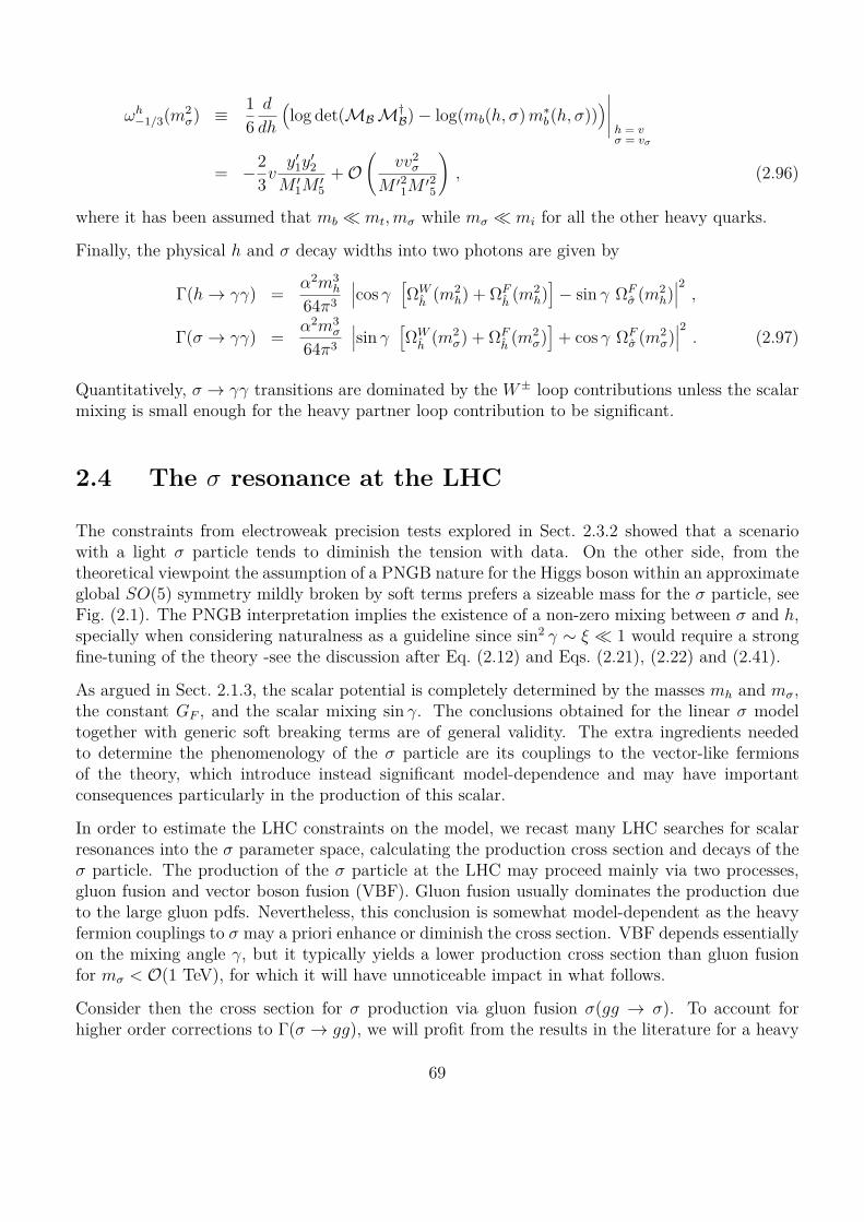
Êh≠1/3(m2

‡) © 16

d

dh

1log det(MB M†

B) ≠ log(mb(h, ‡) múb(h, ‡))

2----- h = v‡ = v‡

= ≠23v

yÕ1y

Õ2

M Õ1M

Õ5

+ OA

vv2‡

M Õ21M

Õ25

B

, (2.96)

where it has been assumed that mb π mt, m‡ while m‡ π mi for all the other heavy quarks.

Finally, the physical h and ‡ decay widths into two photons are given by

�(h æ ““) = –2m3h

64fi3

---cos “Ë�W

h(m2

h) + �Fh

(m2h)

È≠ sin “ �F

‡ (m2h)

---2

,

�(‡ æ ““) = –2m3‡

64fi3

---sin “Ë�W

h(m2

‡) + �Fh

(m2‡)

È+ cos “ �F

‡ (m2‡)

---2

. (2.97)

Quantitatively, ‡ æ ““ transitions are dominated by the W ± loop contributions unless the scalarmixing is small enough for the heavy partner loop contribution to be significant.

2.4 The ‡ resonance at the LHC

The constraints from electroweak precision tests explored in Sect. 2.3.2 showed that a scenariowith a light ‡ particle tends to diminish the tension with data. On the other side, from thetheoretical viewpoint the assumption of a PNGB nature for the Higgs boson within an approximateglobal SO(5) symmetry mildly broken by soft terms prefers a sizeable mass for the ‡ particle, seeFig. (2.1). The PNGB interpretation implies the existence of a non-zero mixing between ‡ and h,specially when considering naturalness as a guideline since sin2 “ ≥ › π 1 would require a strongfine-tuning of the theory -see the discussion after Eq. (2.12) and Eqs. (2.21), (2.22) and (2.41).

As argued in Sect. 2.1.3, the scalar potential is completely determined by the masses mh and m‡,the constant GF , and the scalar mixing sin “. The conclusions obtained for the linear ‡ modeltogether with generic soft breaking terms are of general validity. The extra ingredients neededto determine the phenomenology of the ‡ particle are its couplings to the vector-like fermionsof the theory, which introduce instead significant model-dependence and may have importantconsequences particularly in the production of this scalar.

In order to estimate the LHC constraints on the model, we recast many LHC searches for scalarresonances into the ‡ parameter space, calculating the production cross section and decays of the‡ particle. The production of the ‡ particle at the LHC may proceed mainly via two processes,gluon fusion and vector boson fusion (VBF). Gluon fusion usually dominates the production dueto the large gluon pdfs. Nevertheless, this conclusion is somewhat model-dependent as the heavyfermion couplings to ‡ may a priori enhance or diminish the cross section. VBF depends essentiallyon the mixing angle “, but it typically yields a lower production cross section than gluon fusionfor m‡ < O(1 TeV), for which it will have unnoticeable impact in what follows.

Consider then the cross section for ‡ production via gluon fusion ‡(gg æ ‡). To account forhigher order corrections to �(‡ æ gg), we will profit from the results in the literature for a heavy

69

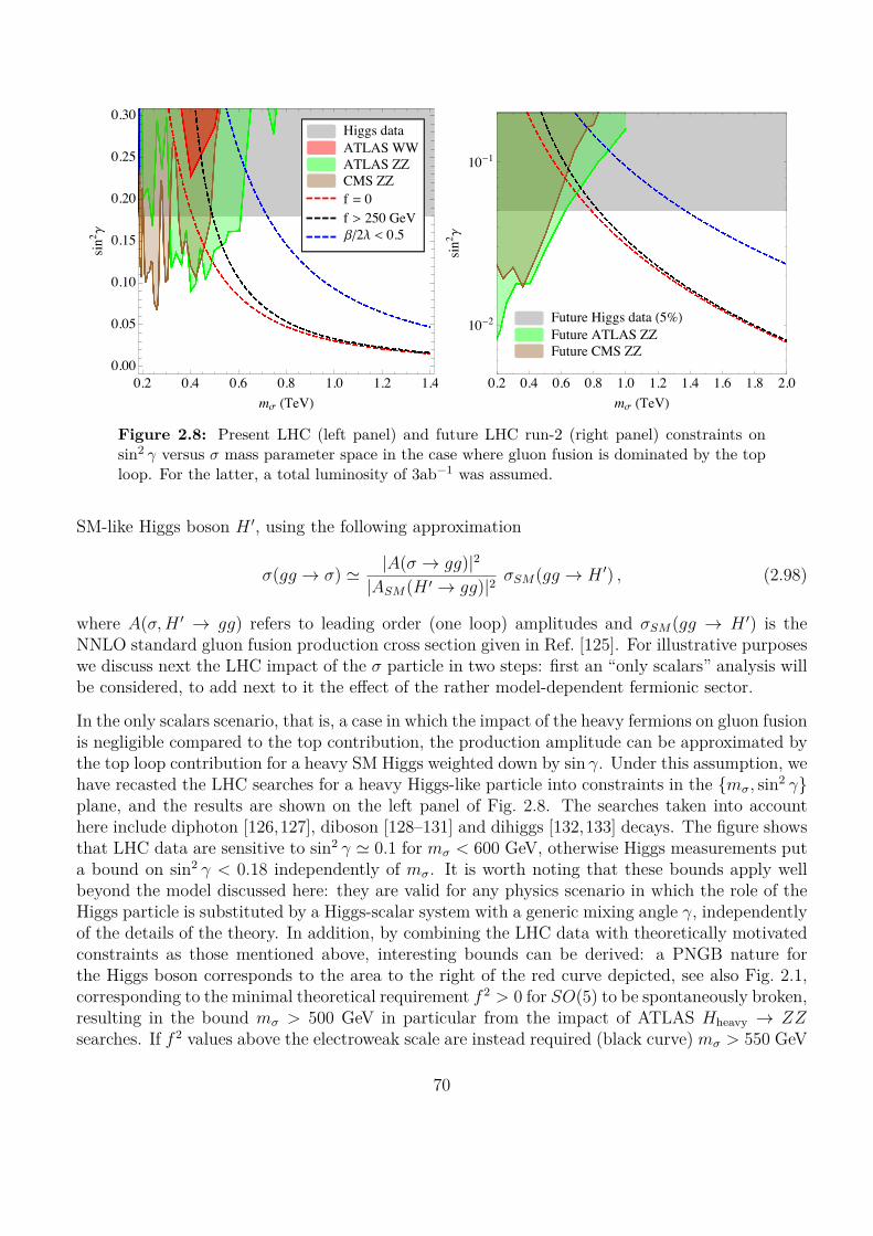
0.2 0.4 0.6 0.8 1.0 1.2 1.40.00

0.05

0.10

0.15

0.20

0.25

0.30

ms HTeVL

sin2 g

Higgs dataATLAS WWATLAS ZZCMS ZZf = 0f > 250 GeVbê2l < 0.5

0.2 0.4 0.6 0.8 1.0 1.2 1.4 1.6 1.8 2.0

10-2

10-1

ms HTeVLsin

2 g

Future Higgs data H5%LFuture ATLAS ZZFuture CMS ZZ

Figure 2.8: Present LHC (left panel) and future LHC run-2 (right panel) constraints onsin2 “ versus ‡ mass parameter space in the case where gluon fusion is dominated by the toploop. For the latter, a total luminosity of 3ab≠1 was assumed.

SM-like Higgs boson H Õ, using the following approximation

‡(gg æ ‡) ƒ |A(‡ æ gg)|2|ASM(H Õ æ gg)|2 ‡SM(gg æ H Õ) , (2.98)

where A(‡, H Õ æ gg) refers to leading order (one loop) amplitudes and ‡SM(gg æ H Õ) is theNNLO standard gluon fusion production cross section given in Ref. [125]. For illustrative purposeswe discuss next the LHC impact of the ‡ particle in two steps: first an “only scalars” analysis willbe considered, to add next to it the e�ect of the rather model-dependent fermionic sector.

In the only scalars scenario, that is, a case in which the impact of the heavy fermions on gluon fusionis negligible compared to the top contribution, the production amplitude can be approximated bythe top loop contribution for a heavy SM Higgs weighted down by sin “. Under this assumption, wehave recasted the LHC searches for a heavy Higgs-like particle into constraints in the {m‡, sin2 “}plane, and the results are shown on the left panel of Fig. 2.8. The searches taken into accounthere include diphoton [126,127], diboson [128–131] and dihiggs [132,133] decays. The figure showsthat LHC data are sensitive to sin2 “ ƒ 0.1 for m‡ < 600 GeV, otherwise Higgs measurements puta bound on sin2 “ < 0.18 independently of m‡. It is worth noting that these bounds apply wellbeyond the model discussed here: they are valid for any physics scenario in which the role of theHiggs particle is substituted by a Higgs-scalar system with a generic mixing angle “, independentlyof the details of the theory. In addition, by combining the LHC data with theoretically motivatedconstraints as those mentioned above, interesting bounds can be derived: a PNGB nature forthe Higgs boson corresponds to the area to the right of the red curve depicted, see also Fig. 2.1,corresponding to the minimal theoretical requirement f 2 > 0 for SO(5) to be spontaneously broken,resulting in the bound m‡ > 500 GeV in particular from the impact of ATLAS Hheavy æ ZZsearches. If f 2 values above the electroweak scale are instead required (black curve) m‡ > 550 GeV

70

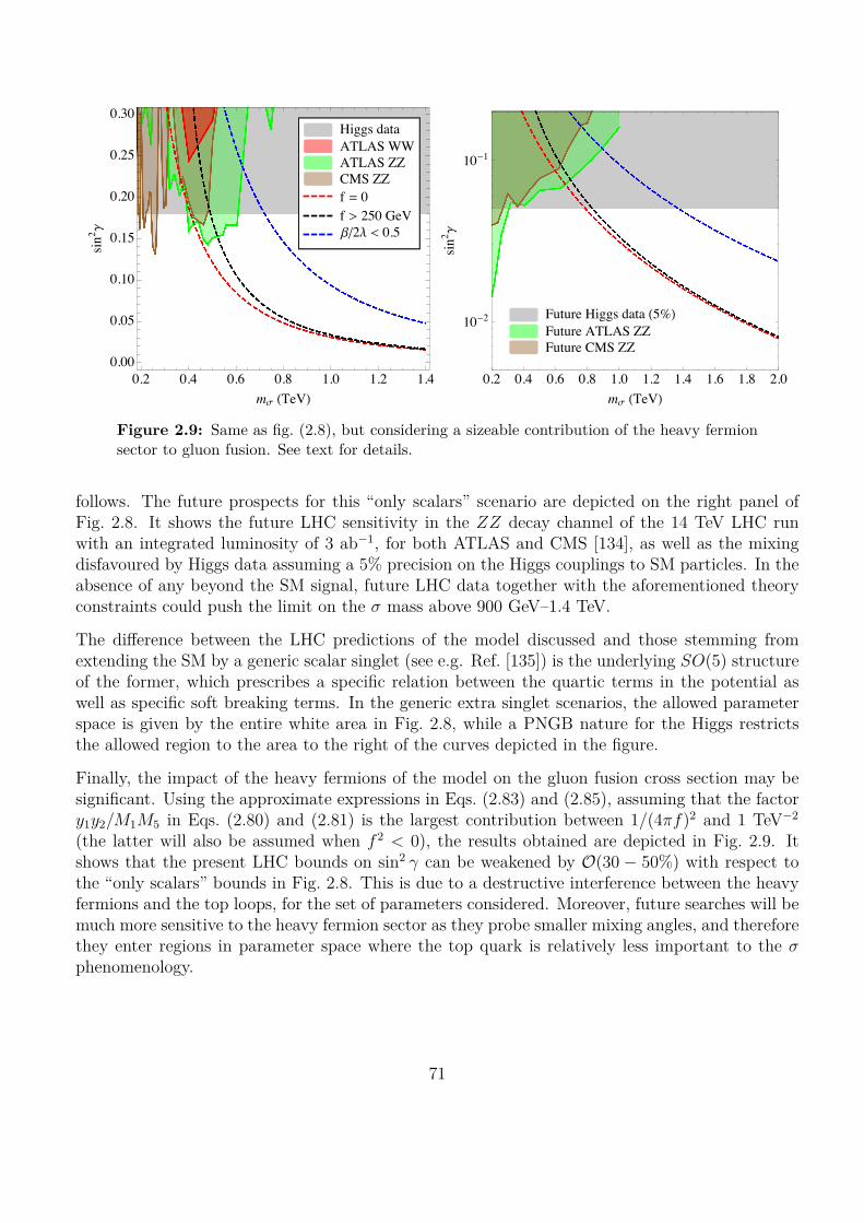
0.2 0.4 0.6 0.8 1.0 1.2 1.40.00

0.05

0.10

0.15

0.20

0.25

0.30

ms HTeVL

sin2 g

Higgs dataATLAS WWATLAS ZZCMS ZZf = 0f > 250 GeVbê2l < 0.5

0.2 0.4 0.6 0.8 1.0 1.2 1.4 1.6 1.8 2.0

10-2

10-1

ms HTeVLsin

2 g

Future Higgs data H5%LFuture ATLAS ZZFuture CMS ZZ

Figure 2.9: Same as fig. (2.8), but considering a sizeable contribution of the heavy fermionsector to gluon fusion. See text for details.

follows. The future prospects for this “only scalars” scenario are depicted on the right panel ofFig. 2.8. It shows the future LHC sensitivity in the ZZ decay channel of the 14 TeV LHC runwith an integrated luminosity of 3 ab≠1, for both ATLAS and CMS [134], as well as the mixingdisfavoured by Higgs data assuming a 5% precision on the Higgs couplings to SM particles. In theabsence of any beyond the SM signal, future LHC data together with the aforementioned theoryconstraints could push the limit on the ‡ mass above 900 GeV–1.4 TeV.

The di�erence between the LHC predictions of the model discussed and those stemming fromextending the SM by a generic scalar singlet (see e.g. Ref. [135]) is the underlying SO(5) structureof the former, which prescribes a specific relation between the quartic terms in the potential aswell as specific soft breaking terms. In the generic extra singlet scenarios, the allowed parameterspace is given by the entire white area in Fig. 2.8, while a PNGB nature for the Higgs restrictsthe allowed region to the area to the right of the curves depicted in the figure.

Finally, the impact of the heavy fermions of the model on the gluon fusion cross section may besignificant. Using the approximate expressions in Eqs. (2.83) and (2.85), assuming that the factory1y2/M1M5 in Eqs. (2.80) and (2.81) is the largest contribution between 1/(4fif)2 and 1 TeV≠2

(the latter will also be assumed when f 2 < 0), the results obtained are depicted in Fig. 2.9. Itshows that the present LHC bounds on sin2 “ can be weakened by O(30 ≠ 50%) with respect tothe “only scalars” bounds in Fig. 2.8. This is due to a destructive interference between the heavyfermions and the top loops, for the set of parameters considered. Moreover, future searches will bemuch more sensitive to the heavy fermion sector as they probe smaller mixing angles, and thereforethey enter regions in parameter space where the top quark is relatively less important to the ‡phenomenology.

71

Coe�cient Leading Order in f/M

ZqL

31 + �2

1M2

5+ �Õ2

1M Õ2

5

4

ZtR

11 + �2

2M2

5+ �2

3M2

1

2

ZbR

31 + �Õ2

2M Õ2

5+ �Õ2

3M Õ2

1

4

Table 2.2: Table with the definitions for the renormalization factors.

The 750 GeV di-photon excess

In 2015 both ATLAS [136] and CMS [137] reported the mild 750 GeV di-photon excess. Eventhough it disappeared in the updated results we have analysed weather the ‡ resonance could havebeen responsible for generating this excess.

It turned out to be highly unlikely because of the constraints imposed on the scalar couplings bythe approximate SO(5) symmetry of the scalar potential, as well as the uniqueness of the signal,as explained next.

Since the decay ‡ æ ““ is loop induced, the corresponding branching ratio tends to be very small.In order to be able to account for the excess observed, the h≠‡ mixing needs to be tiny, so that forinstance the WW and ZZ channels are suppressed and the loop-induced processes may dominatethe decay. This requires sin2 “ π (mh/m‡)2 ƒ 0.03, which Eq. (2.21) shows to require on one sidef 2 < 0 –for which the Higgs cannot be interpreted as a PNGB, and on the other a very small andfine-tuned – value as –2 Ã —2 sin2(2“); overall a very unnatural scenario.

Furthermore, since the mixing is so small, the top loop essentially does not contribute to theproduction and decay anymore. Hence, to obtain a large enough �(‡ æ ““) and �(‡ æ gg) thefermion content needs a higher multiplicity than what is assumed in this analysis, as well as largeYukawa couplings, since ‡ mainly couples to T1 and T5 with electric charges 2/3. Even assumingsuch an extreme and extended configuration, the stability of the potential could become a veryserious issue as the fermion contribution to the beta function of the quartic couplings is negative.Additional field content would then be possibly required to compensate for this e�ect, making themodel extremely ad hoc. Therefore, we found no compelling argument to interpret the 750 GeVexcess as corresponding to the ‡ scalar studied here.

2.5 d Æ 6 Fermionic E�ective Lagrangian

The linear model described is renormalizable and valid for any mass range of the fermionic and/orscalar exotic fields. Two simplifying limits are specially interesting: i) the heavy fermion regime,M ∫ m‡ ∫ v, where M generically represents the exotic fermionic scales Mi in Eq. (2.30); ii)the heavy singlet regime, m‡ ∫ M ∫ v. We have concentrated on the first scenario, considering

72

Operator ci Leading Order in f/M

dim 4qL

ÊH tR ≠yt ≠1

y1�1�3M1M5

2Z≠1/2

qLZ≠1/2

tR

qL H bR ≠yb ≠1

yÕ1�Õ

1�Õ3

M Õ1M Õ

5

2Z≠1/2

qLZ≠1/2

bR

dim 5‡ (qL

ÊHtR) ct‡1

yt

M5

1y2

�2�3

≠1y1

�2�3M1M5

+ y2�2�3M2

1

2Z≠1

tR

2

‡ (qLHbR) cb‡1

ybM Õ

5

1yÕ

2�Õ

2�Õ

3≠

1yÕ

1�Õ

2�Õ3

M Õ1M Õ

5+ yÕ

2�Õ

2�Õ3

M Õ21

2Z≠1

bR

2

dim 6

‡2 (qLÊHtR) ct

‡2

≠ yt

M1M5

3y1y2 ≠

1y1y2

12 �2

2M2

5+ �2

3M2

1

2+ 3y2

2�22+y2

1�23

2M1M5

2Z≠1

tR

+2 �22�2

3M1M5

1y2

1M2

5+ 2y1y2

M5M1+ y2

2M2

1

2Z≠2

tR

4

‡2 (qLHbR) cb‡2

≠ ybM Õ

1M Õ5

3yÕ

1yÕ2 ≠

1yÕ

1yÕ2

12 �Õ2

2M Õ2

5+ �Õ2

3M Õ2

1

2+ 3yÕ2

2�Õ22+yÕ2

1�Õ23

2M Õ1M Õ

5

2Z≠1

bR

+2�Õ22�Õ2

3M Õ

1M Õ5

1yÕ2

1M Õ2

5+ 2yÕ

1yÕ2

M Õ5M Õ

1+ yÕ2

2M Õ2

1

2Z≠2

bR

4

|H|2 (qLÊHtR) ct

H2

≠ yt

M1M5

32y1y2 ≠

12y1y2

�23

M21

+ y21

�23

M1M5

2Z≠1

tR

≠1y1y2

�21

M25

+ y212

�21

M1M5

2Z≠1

qL

4

|H|2 (qLHbR) cbH2

≠ ybM Õ

1M Õ5

32yÕ

1yÕ2 ≠

12yÕ

1yÕ2

�Õ23

M Õ21

+ yÕ21

�Õ23

M Õ1M Õ

5

2Z≠1

bR

≠1yÕ

1yÕ2

�Õ21

M Õ25

+ yÕ21

2�Õ2

1M Õ

1M Õ5

2Z≠1

qL

4

(H†iΩæD µ H)(qL“µqL) c(1)

L14

3y2

1�21

M21 M2

5≠ yÕ2

1�Õ21

M Õ21M Õ2

5

4Z≠1

qL

(H†iΩæD i

µ H)(qL· i“µqL) c(3)L ≠1

4

3y2

1�21

M21 M2

5+ yÕ2

1�Õ21

M Õ21M Õ2

5

4Z≠1

qL

(H†iΩæD µ H)(tR“µtR) ct

R 0

(H†iΩæD µ H)(bR“µbR) cb

R 0

i(ÊH†Dµ H)(tR“µbR) ctbR 0

Table 2.3: Leading order low-energy e�ective operators induced and their coe�cients. Notethat the Yukawa couplings defined in the two first rows appear as well in coe�cients of somehigher order operators. The renormalization factors present have been defined in Table 2.2.Those operators made out exclusively of SM fields have been written in the Warsaw basis [88].

73

a not-so-heavy extra singlet in the spectrum and its phenomenological consequences. The secondlimit is instead interesting to elucidate the connection between the linear (weak) and non-linear(strong) BSM physics scenarios: the m‡ æ Œ regime should lead to the non-linear scenariosusually explored in the literature about composite Higgs; it will be discussed in detail in Chapter3.

When condition i) is satisfied, some important low-energy e�ects (and model dependencies) inducedby the exotic fermions are easily inferred by integrating them out. The procedure is quite lengthy;here only the resulting mass-dimension (d) 4, 5 and 6 e�ective operators and their coe�cients aresummarized. For energies E < M , the e�ective Lagrangian describing the d Æ 6 interactions offermions with gauge and scalar fields can be written as

Leff = qLi /D qL + tRi /D tR + bRi /D bR +ÿ

i

ciOi , (2.99)

where the set {Oi} includes operators of dimension four (for which the induced coe�cients arethe leading contributions to the top and bottom Yukawa couplings), five and six. We will use the“Warsaw basis” [88] below.

In most models (for instance in composite Higgs ones) it is reasonable to assume that the goldstoneboson scale f and the scalar vevs all satisfy f , v , v‡ π M . In what follows we will thus assumef/M π 1 for simplicity, while � ¥ M will be considered with � denoting generically the composite�i scales in Eq. (2.30). The light field kinetic energies get contributions which require wave functionrenormalization in order to recover canonically normalized kinetic energies,

qL æ Z≠1/2qL

qL , (2.100)

qR æA

Z≠1/2tR

00 Z≠1/2

bR

B AtR

bR

B

, (2.101)

where Z≠1/2tR

and Z≠1/2bR

are given in Table 2.2. The operators obtained and their coe�cientsresulting after those redefinitions, at leading order in f/M , are shown in Table 2.3, where thefollowing definitions have been used,

(H†iΩæD µ H) © i

1H†(≠æDµH) ≠ (H†Ω≠Dµ)H

2,

(H†iΩæD i

µ H) © i1H†· i(≠æDµH) ≠ (H†Ω≠Dµ)· iH

2.

In writing Eq. (2.99) and Table 2.3 the unshifted scalar fields have been assumed. This factintroduces a potential subtlety that we discuss next. Consider for instance the top and bottomquark masses corresponding to the first two operators in the table, which are their respectiveYukawa couplings: when the Higgs gets a vev, mass terms for the light quarks are generated.Additional contributions to the light quark masses stem however from the next six operators inthe list, for ‡ = È‡Í and H = ÈHÍ. The corrections induced in the top and bottom mass areof higher order in f/M , though, and do not need to be retained when working at leading order.Finally,

mt = vÔ2

Ay1�1�3

M1M5

B1

Ú11 + �2

1M2

5+ �Õ2

1M Õ2

5

2 11 + �2

2M2

5+ �2

3M2

1

2

A

1 + OA

f

M

BB

,

74

mb = vÔ2

AyÕ

1�Õ1�Õ

3M Õ

1MÕ5

B1

Ú11 + �2

1M2

5+ �Õ2

1M Õ2

5

2 11 + �Õ2

2M Õ2

5+ �Õ2

3M Õ2

1

2

A

1 + OA

f

M

BB

.

The same reasoning applies to other couplings. For example the fermion-‡ coupling via the Ot‡1 op-

erator [88] would get corrections proportional to ct‡2È‡Í –see Table (2.3)– which are of higher order

in the f/M expansion, and can thus be disregarded when restraining to the leading contributions.

75

3

The linear-non-linear frontier for theGoldstone Higgs

A complete renormalizable model of Goldstone Higgs was constructed in Chapter 2. Its scalar partis a linear sigma model including a new singlet scalar ‡. The procedure and first steps to obtainthe non-linear e�ective Lagrangian were developed. In particular we have derived the leading orderlow-energy e�ective operators composed of the SM fields and scalar ‡. In this section we explorethe divide between linear and non-linear regimes by varying the mass of the extra scalar: a light ‡particle corresponds to a weakly coupled regime, while in the high mass limit the theory will fallback onto the e�ective non-linear construction.

The e�ective low-energy e�ective Lagrangian in a general case contains a large number of couplings.For the generic SO(5)/SO(4) construction, a very reduced subset of those couplings, constitutinga complete basis of bosonic operators, was established in Ref. [70]. Here we will focus on theparticular case of the minimal SO(5) sigma model, leading to an even more reduced subset ofoperators –the benchmark low-energy e�ective Lagrangian. We consider here both bosonic andfermionic operators. The leading linear corrections and the leading dependence on the explicitSO(5)-breaking mechanism will be determined as well.

While the bosonic couplings are general, the fermionic part may instead be quite model-dependent.We will address the problem in two approaches:

• A rather model independent one in which the field content of the SM is augmented exclusivelyby a singlet scalar within the minimal SO(5) setup, while the leading phenomenologicalimpact of heavy fermions is encoded in an e�ective Yukawa coupling of the SM fields that wewill define. This e�ective operator will serve to parametrise and disentangle among di�erentchoices of BSM fermion embeddings.

• In a second step, we consider the heavy fermion representations of the complete modeldescribed in the previous chapter. This sector will be integrated out explicitly.

By furthermore keeping track of the linear and heavy-fermion corrections, the analysis will provide

76

Figure 3.1: Schematic fermion mass operator at low scales with arbitrary insertions of thescalar fields.

candles to identify whether a renormalizable ultraviolet completion exists in nature or alternativelyan underlying composite mechanism is at work at high-energy, analogous to QCD for the chiraldynamics involving pions.

3.1 Model independent analysis

The scalar sector has been fully defined in the previous chapter by Eqs. (2.3, 2.8) and remainsuniversal.

Consider now the fermion sector. A generic feature is that the phenomenological constraints onpartial compositeness require additional vector-like fermions, which couple and act as mediatorsamong the SM fields. The exact form of the e�ective coupling is model-dependent and variesaccording to how the SM fermions are embedded in SO(5). We will obviate until Sect. 3.2 thedetails of the heavy fermion spectrum, and use instead in this section a simplified –e�ective–approach to the dominant fermion-induced e�ects.

The fermionic part of the Lagrangian in Eq. (2.1) will be written as the sum of two terms,

Lf = Lkinf,SM + LYuk

f , (3.1)

where Lkinf,SM comprises the kinetic terms for only SM fermions.

The schematic e�ective Yukawa coupling in the presence of the ‡ particle is presented in figure 3.1.It follows that at low energies it is possible to write an e�ective Yukawa Lagrangian in terms ofonly the SM fermions, plus h and ‡, which respects electroweak gauge invariance but not SO(5)invariance,

LYukf © y0

f O(n,m)Yuk,f + · · · + h.c. , (3.2)

77

Fermion representation (qL-qR) Yukawa interactions y0f O(n,m)

Yuk

5-1, 5-10, 10-5 yO(0,0)Yuk

5-5, 10-10, 14-10, 10-14, 14-1 yO(1,0)Yuk

14-14 3yO(1,0)Yuk ≠ 2yÕO(1,1)

Yuk + 8yÕO(3,0)Yuk

14-5 yO(0,0)Yuk + yÕO(2,0)

Yuk

5-14 yO(0,0)Yuk + yÕO(0,1)

Yuk ≠ 4yÕO(2,0)Yuk

Table 3.1: Yukawa operators corresponding to particular embeddings (see e.g. Ref [16]) of aSM quark doublet qL and right-handed qR fermion (either up-type or down-type right-handedquark) into SO(5). The coe�cients y, yÕ refer to distinct possible relative weights of SO(5)invariant operators allowed by the models

where the constant y0f is a model-dependent coe�cient 1 and we define the e�ective Yukawa

operator for a given fermion f as

O(n,m)Yuk,f © qL

ÊH fRA

‡

f

Bn A2H†H

f 2

Bm

. (3.3)

The ellipses in Eq. (3.2) refer to other SM fermion operators and possibly extra model-dependentterms coming from the heavy fermion sector.

In the literature of composite Higgs models the notation MCHMA≠B≠C is often used to indicatetheir fermion composition, with A, B, C indicating the SO(5) representation in which the SMdoublet qL, up-type right-handed and down-type right-handed fermions are embedded, respec-tively; else, when only one subindex appears as in MCHMA it is understood to be of the typeMCHMA≠A≠A. Table 3.1 summarizes the {n, m} parameter values for di�erent models. We do nottake into account the models with spinorial SO(5) embeddings [9] as they are phenomenologicallyexcluded [10].

Eq. (3.3) assumes that a given fermion mass corresponds to a single set of {n, m} values. This isoften the case; for instance, the top and bottom Yukawa couplings in the MCHM5≠1≠1 model ofthe previous chapter correspond to O(0,0)

Yuk , while in the MCHM5 scenario they both correspond toO(1,0)

Yuk (see e.g. Ref. [69]). Notice that, for these cases with a single Yukawa operator, the globalcoe�cients and suppression scales in Eqs. (3.2)-(3.3) are constrained by the fermion masses andtherefore do not constitute any additional model dependence.

Nevertheless, in some scenarios a given fermion mass results instead from combining several op-erators of the type in Eq. (3.3) with di�erent {n, m} values. The procedure derived can be easily

1The superscript 0 indicates that y0f only encodes the leading contributions induced by the heavy fermionic

sector.

78

extended to encompass it. A model-dependence remains then in the relative size of the y and yÕ

weights in Table 3.1. An example is the MCHM14≠14≠10 scenario [16] in which di�erent sets of{n, m} values are involved in generating the top mass, while the bottom mass only requires set{n, m} = {1, 0}. The cases of single and of multiple Yukawa operators contributing to a given masswill be further considered explicitly below. We focus in what follows on the top Yukawa couplingunless otherwise explicitly stated, while the conclusions to be obtained are easily generalized toall light fermions.

3.1.1 Polar coordinates

Armed with the tools described, it is quite straightforward to derive the benchmark bosonic La-grangian as well as the leading couplings involving fermions. To this aim, it is convenient to rewritethe scalar degrees of freedom in polar coordinates,

‡ © fl cÏ , (3.4)

H © 1Ô2

fl U sÏ , (3.5)

with cÏ © cos Ï/f , sÏ © sin Ï/f , and U(x) © exp{ifi(x)·/f} as usual being the Goldstone matrixcorresponding to the longitudinal components of the electroweak gauge bosons. This notationdi�ers from the one used before, as the f scale instead of v divides the field fi. In order to obtainthe usual v scale suppression and the canonical kinetic term for the would-be-Goldstones afterthe EWSB the fi field has to be rescaled by f/v. Having this in mind, we will keep the f scalesuppression in what is following for simplicity. In this notation the scalar Lagrangian in Eq. (2.3)with the potential defined in Eq. (2.8) reads

Ls = 12ˆµfl ˆµfl + fl2

2f 2

C

ˆµÏ ˆµÏ ≠ f 2

2 s2Ï ÈVµVµÍ

D

≠ ⁄(fl2 ≠ f 2)2 ≠ –f 3fl cÏ + —f 2fl2s2Ï. (3.6)

The e�ective top Yukawa operator in Eqs. (3.2) and (3.3) is then given by

y0t O(n,m)

Yuk,t = y0tÔ2

(qLUP+qR)flA

fl

f

Bn+2m

cnÏs2m+1

Ï , (3.7)

where the right-handed SM fermions have been gathered in a formal doublet qR © (tR, bR), withP+ © diag(1, 0) (P≠ = diag(0, 1)) being a projector onto the up-type (down-type) right-handedSM fermions.

The fl and Ï fields will develop vevs,

fl æ fl + ÈflÍ , Ï æ h + ÈÏÍ , (3.8)

where at the minimum of the potential the Ï field corresponds to

cosA

ÈÏÍf

B

= ≠ –

2—

A

1 + —

2⁄

B≠1/2

. (3.9)

79

The connection between the vevs of the fields in the linear and polar parametrisations is

ÈflÍ =Ò

È‡Í2 + 2 ÈHÍ2, ÈÏÍ = f tan≠1AÔ

2 ÈHÍÈ‡Í

B

. (3.10)

The scalar resonance, which in the linear parametrisation is customarily denoted ‡, is traded byfl in the polar parametrisation, with mfl = m‡ exactly as expected for a physical observable, whilethe Higgs resonance h corresponds now to the excitation of the Ï field, see Eq. 3.8.

Finally, as the pure gauge Lagrangian Lg and the weak coupling to fermions are not modified, thecoe�cient of the Wµ mass term in Eq. (3.6) allows to identify the electroweak scale v in terms ofthe Lagrangian parameters:

v2 = ÈflÍ2 sin2A

ÈÏÍf

B

. (3.11)

3.1.2 Expansion in 1/⁄

The scalar quartic coupling ⁄ can be conventionally traded by the fl mass, given by m2fl ƒ 8⁄f 2

for negligible – and —, the non-linear model would be recovered in the limit mfl ∫ f , thatis ⁄ æ Œ. Varying the fl mass (that is, ⁄) allows to switch from the regime of perturbativeultraviolet completion to the non-linear one assumed in models in which the Higgs particle is alow-energy remnant of some strong dynamics. We will explore this limit next.

The exact equation of motion for fl reads

⇤fl≠ fl

f 2

C

ˆµÏ ˆµÏ ≠ f 2

2 s2Ï ÈVµVµÍ

D

+ 4⁄fl(fl2 ≠ f 2) + –f 3cÏ ≠ 2—flf 2s2Ï

+ (n + 2m + 1)A

y0tÔ2

qLUP+qR + h.c.

B

cnÏs2m+1

Ï

Afl

f

Bn+2m

= 0, (3.12)

where ⇤ © ˆµ ˆµ. In a 1/⁄ expansion, the fl field can be expressed as

fl © fl0 + fl1/⁄ + fl2/⁄2 + . . .

where the leading terms are given by

fl0 = f, (3.13)

fl1 = f

4

5 12f 4 ˆµÏ ˆµÏ ≠ 1

4f 2 ÈVµVµÍ s2Ï ≠ 1

2–cÏ + —s2Ï

≠ (n + 2m + 1)2f 3

Ay0

tÔ2

qLUP+qR + h.c.

B

cnÏs2m+1

Ï

6, (3.14)

and subsequent ones can be written as polynomial functions of fl1. Substituting these in Eq. (3.6)yields the 1/⁄n Lagrangian corrections,

L = L0 + L1/⁄ + L2/⁄2 + . . . , (3.15)

80

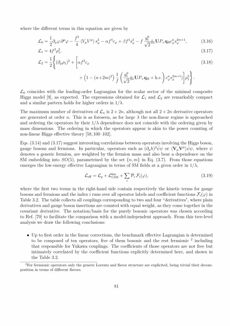
where the di�erent terms in this equation are given by

L0 = 12ˆµÏ ˆµÏ ≠ f 2

4 ÈVµV µÍ s2Ï ≠ –f 4cÏ + —f 4s2

Ï ≠ fy0

tÔ2

qLUP+qRcnÏs2m+1

Ï , (3.16)

L1 = 4f 2fl21, (3.17)

L2 = 12

Y]

[(ˆµfl1)2 +C

–f 2cÏ (3.18)

+11 ≠ (n+2m)2

2 1f

Ay0

tÔ2

qLUP+qR + h.c.

B

cnÏs2m+1

Ï )D

fl21

Z^

\ .

L0 coincides with the leading-order Lagrangian for the scalar sector of the minimal compositeHiggs model [9], as expected. The expressions obtained for L1 and L2 are remarkably compactand a similar pattern holds for higher orders in 1/⁄.

The maximum number of derivatives of Ln is 2 + 2n, although not all 2 + 2n derivative operatorsare generated at order n. This is as foreseen, as for large ⁄ the non-linear regime is approachedand ordering the operators by their 1/⁄ dependence does not coincide with the ordering given bymass dimensions. The ordering in which the operators appear is akin to the power counting ofnon-linear Higgs e�ective theory [58,100–102].

Eqs. (3.14) and (3.17) suggest interesting correlations between operators involving the Higgs boson,gauge bosons and fermions. In particular, operators such as (ˆµh)2ÂÂ or ÈVµVµÍÂÂ, where Âdenotes a generic fermion, are weighted by the fermion mass and also bear a dependence on theSM embedding into SO(5), parametrised by the set {n, m} in Eq. (3.7). From those equationsemerges the low-energy e�ective Lagrangian in terms of SM fields at a given order in 1/⁄,

Le� = Lg + Lkinf,SM +

ÿ

i

Pi Fi(Ï), (3.19)

where the first two terms in the right-hand side contain respectively the kinetic terms for gaugebosons and fermions and the index i runs over all operator labels and coe�cient functions Fi(Ï) inTable 3.2. The table collects all couplings corresponding to two and four “derivatives", where plainderivatives and gauge boson insertions are counted with equal weight, as they come together in thecovariant derivative. The notation/basis for the purely bosonic operators was chosen accordingto Ref. [70] to facilitate the comparison with a model-independent approach. From this tree-levelanalysis we draw the following conclusions:

• Up to first order in the linear corrections, the benchmark e�ective Lagrangian is determinedto be composed of ten operators, five of them bosonic and the rest fermionic 2 includingthat responsible for Yukawa couplings. The coe�cients of those operators are not free butintimately correlated by the coe�cient functions explicitly determined here, and shown inthe Table 3.2.

2For fermionic operators only the generic Lorentz and flavor structure are explicited, being trivial their decom-position in terms of di�erent flavors.

81

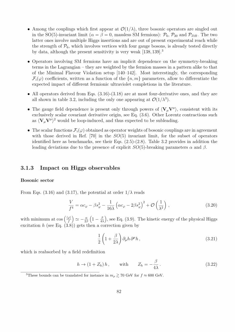
• Among the couplings which first appear at O(1/⁄), three bosonic operators are singled outin the SO(5)-invariant limit (– = — = 0, massless SM fermions): P6, P20 and PDH . The twolatter ones involve multiple Higgs insertions and are out of present experimental reach whilethe strength of P6, which involves vertices with four gauge bosons, is already tested directlyby data, although the present sensitivity is very weak [138,139].3

• Operators involving SM fermions have an implicit dependence on the symmetry-breakingterms in the Lagrangian – they are weighted by the fermion masses in a pattern alike to thatof the Minimal Flavour Violation setup [140–142]. Most interestingly, the correspondingFi(Ï) coe�cients, written as a function of the {n, m} parameters, allow to di�erentiate theexpected impact of di�erent fermionic ultraviolet completions in the literature.

• All operators derived from Eqs. (3.16)-(3.18) are at most four-derivative ones, and they areall shown in table 3.2, including the only one appearing at O(1/⁄3).

• The gauge field dependence is present only through powers of ÈVµVµÍ, consistent with itsexclusively scalar covariant derivative origin, see Eq. (3.6). Other Lorentz contractions suchas ÈVµVµÍ2 would be loop-induced, and thus expected to be subleading.

• The scalar functions Fi(Ï) obtained as operator weights of bosonic couplings are in agreementwith those derived in Ref. [70] in the SO(5) invariant limit, for the subset of operatorsidentified here as benchmarks, see their Eqs. (2.5)-(2.8). Table 3.2 provides in addition theleading deviations due to the presence of explicit SO(5)-breaking parameters – and —.

3.1.3 Impact on Higgs observables

Bosonic sector

From Eqs. (3.16) and (3.17), the potential at order 1/⁄ reads

V

f 4 = –cÏ ≠ —s2Ï ≠ 1

16⁄

1–cÏ ≠ 2—s2

Ï

22+ O

3 1⁄2

4, (3.20)

with minimum at cos1

ÈÏÍf

2ƒ ≠ –

2—

11 ≠ —

4⁄

2, see Eq. (3.9). The kinetic energy of the physical Higgs

excitation h (see Eq. (3.8)) gets then a correction given by

12

A

1 + —

2⁄

B

ˆµh ˆµh , (3.21)

which is reabsorbed by a field redefinition

h æ (1 + Zh) h , with Zh = ≠ —

4⁄. (3.22)

3These bounds can be translated for instance in mfl & 70 GeV for f ¥ 600 GeV.

82

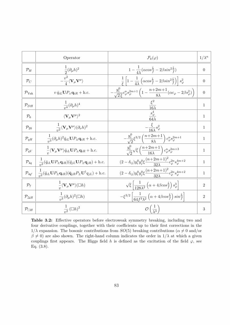
Operator Fk(Ï) 1/⁄n

PH12(ˆµh)2 1 ≠ 1

4⁄(–cos h

f ≠ 2—sin2 hf ) 0

PC ≠v2

4 ÈVµVµÍ 1›

51 ≠ 1

4⁄

1–cos h

f ≠ 2—sin2 hf

26s2

Ï 0

PYuk v qiLUP±qiR + h.c. ≠ y0iÔ2 ›

cnÏs2m+1

Ï

31 ≠ n+2m+1

8⁄(–cÏ ≠ 2—s2

Ï)4

0

PDH1v4 (ˆµh)4 ›2

16⁄1

P6 ÈVµVµÍ2 s4Ï

64⁄1

P201v2 ÈVµVµÍ(ˆ‹h)2 ≠ ›

16⁄s2

Ï 1

PqH1v3 (ˆµh)2qiLUP±qiR + h.c. ≠ y0

iÔ2

›3/23

n+2m+18⁄

4cn

Ïs2m+1Ï 1

PqV1v

ÈVµVµÍqiLUP±qiR + h.c.y0

iÔ2

Ô›

3n+2m+1

16⁄

4cn

Ïs2m+3Ï 1

P4q1v2 (qiLUP±qiR)(qjLUP±qjR) + h.c. (2 ≠ ”ij)y0

i y0j ›

(n+2m+1)2

32⁄c2n

Ï s4m+2Ï 1

P4qÕ1v2 (qiLUP±qiR)(qjRP±U†qjL) + h.c. (2 ≠ ”ij)y0

i y0j ›

(n+2m+1)2

32⁄c2n

Ï s4m+2Ï 1

P71v

ÈVµVµÍ(⇤h)Ô

›5 1

128⁄2

1– + 4—cos h

f

2s3

Ï

62

P�H1v3 (ˆµh)2(⇤h) ≠›3/2

5 164f3⁄2

1– + 4—cos h

f

2sin h

f

62

P⇤H1v2 (⇤h)2 O

3 1⁄3

43

Table 3.2: E�ective operators before electroweak symmetry breaking, including two andfour derivative couplings, together with their coe�cients up to their first corrections in the1/⁄ expansion. The bosonic contributions from SO(5) breaking contributions (– ”= 0 and/or— ”= 0) are also shown. The right-hand column indicates the order in 1/⁄ at which a givencouplings first appears. The Higgs field h is defined as the excitation of the field Ï, seeEq. (3.8).

83

The scalar sector depends on four independent parameters explicitated in Eq. (2.19), with theonly di�erence that the mass of the heavy scalar is labelled mfl.

In the non-linear limit ⁄ æ Œ the fl field decouples from the spectrum and the scalar sector woulddepend on just three renormalized parameters. It is now possible to foresee the impact of thelinear corrections in terms of mass dependence. Precisely because the large ⁄ and mfl limits are incorrespondence, dimensional arguments suggest the equivalence

1⁄

∆ m2h

m2fl

ƒ —›

4⁄, (3.23)

as the expansion parameter, as it follows from the expressions for the scalar masses in the smallexplicit breaking limit Eq. (2.17). In other words, the linear corrections are expected to be pro-portional to the two small parameters — and › and thus doubly suppressed.

The modification of the Higgs – gauge boson coupling can be parametrised by ŸV and can beextracted for instance from the expression for Higgs to WW decay width as

�(h æ WW ú) © �SM(h æ WW ú) Ÿ2V .

A generic expectation is the departure of ŸV from 1. Indeed, the coupling between the Higgs andthe gauge bosons which stems from the Lagrangian Eqs. (3.15)-(3.18) at order 1/⁄ is that encodedin the operator PC in Table 3.2 and reads

LhV V = ≠A

12

Ò1 ≠ › + —

8⁄

(2 ≠ ›)›Ô1 ≠ ›

B

ÈVµV µÍ vh , (3.24)

or in other wordsŸV =

Ò1 ≠ › + —›

2⁄

(1 ≠ ›/2)Ô1 ≠ ›

. (3.25)

Assuming for illustrative purposes O(›) ≥ O(1/⁄) and expanding up to second order in theseparameters, the result simplifies to

ŸV ƒÒ

1 ≠ › + —›

2⁄. (3.26)

The first term on the right-hand side of this equation is the well-known correction present innon-linear scenarios [9], while the second term encodes the linear correction linked to the scale ofultraviolet completion, which in terms of physical parameters we predict to be given by

Ÿ2V ƒ 1 ≠ › + 4m2

h

m2fl

, (3.27)

where Eq. (3.23) has been used. Higher order corrections are expected to be very small, as they willstem from operators with at least 4 derivatives. For instance, the first extra tree-level contributionto ŸV is the 1/⁄2 weight of the operator P7 in Table 3.2,

”Ÿ2V ƒ 1

2Ô

2GF

m2h

m4fl

.

84

Fermionic sector

Consider first the case in which the fermion mass is generated by a single Yukawa operator O(n,m)Yuk,f ,

see Eqs. (3.2) and (3.3). From the Lagrangian in Eqs. (3.15)-(3.18), and more specifically from theYukawa operator in the third line of Table 3.2, an expression for the fermion mass follows afterapplying Eqs. (3.8) and Eq. (3.22),

LYukf ∏ ≠mf fLfR + h.c. , mf ƒ y0

fÔ2

fÒ

› (1 ≠ ›)n/2›m

A

1 + n1

›(1 ≠ ›)m2

h

m2fl

B

. (3.28)

The renormalization scheme is now enlarged to the fermion sector choosing as observable preciselythe fermion masses. The prediction that follows for the Higgs coupling to a given fermion f,

Lh� © ≠gh� h fLfR + h.c. , (3.29)

takes then the form

gh� ƒ y0fÔ2

(1 ≠ ›)n≠12 ›m

;(1 + 2m)(1 ≠ ›) ≠ n› + —

›(1 ≠ ›)m2

h

m2fl

◊ (3.30)

◊Ë(1 + 2m + n)›(1 ≠ ›)(2 ≠ ›) + n (1 + 2m(1 ≠ ›) ≠ n›)

È<.

Encoding the deviations with respect to the SM expectations through the conventional Ÿf param-eter,

Ÿf © gh�/gSMh� , (3.31)

where gSMh� = mf/v, the exact and somewhat lengthy expression for Ÿf up to order 1/⁄ follows.

The latter can be simply recast assuming again O(›) ≥ O(1/⁄), leading to

Ÿf ƒ (1 + 2m)(1 ≠ ›) ≠ n›Ô1 ≠ ›

+ (2 + 4m + 3n) m2h

m2fl

, (3.32)

where once again Eq. (3.23) has been used. It is straightforward to check that the first termon the right-hand side of this equation reproduces well-known Ÿf results for di�erent models inthe literature, which assume a non-linear realization. The second term gives instead the leadinglinear corrections. For instance, this equation leads to the following results for the MCHM5≠1≠1(corresponding to n = m = 0 in our parametrisation) and MCHM5 (corresponding to n = 1,m = 0):

ŸMCHM5≠1≠1f ƒ

Ò1 ≠ › + 2m2

h

m2fl

, ŸMCHM5f ƒ 1 ≠ 2›Ô

1 ≠ ›+ 5m2

h

m2fl

. (3.33)

obtaining again at order 1/⁄ a correction doubly suppressed as proportional to both — and ›, seeEq. (3.23).

Consider next the case in which a given fermion mass corresponds to the combination of severalSO(5) invariant Yukawa operators, instead of just one as developed above,

LYukf = ≠ c(n,m) O(n,m)

Yuk,f + · · · + h.c., (3.34)

85

where c(n,m) are related to the generators of SO(5) and the fermion embedding in a given model.The procedure is still quite straightforward. The fermion mass will be a sum of contributionssimilar to that in Eq. (3.28) weighted by the coe�cients c(n,m), and a similar combination protocolwill apply to the obtention of the fermion-Higgs coupling gh� and Ÿf . As an example, consider theMCHM14≠14≠10 scenario [16], in which the third family quark doublet and the right-handed topare embedded each in a 14-plet of SO(5), denoted QL and UR respectively, while the right-handedbottom is included in a 10-plet representation denoted DR. Two SO(5) invariant operators [16]contribute in this case to the top quark mass,

yu„†QLUR„ ≠ yu(„†QL„)(„†UR„) æ 3yuO(1,0)Yuk ≠ yu

12O(1,1)

Yuk ≠ 8O(3,0)Yuk

2, (3.35)

leading to

ŸMCHM14≠14≠10t ƒ yu(3 ≠ 6›) + 2yu(4 ≠ 23› + 20›2)Ô

1 ≠ › (3yu + 2yu(4 ≠ 5›)) + 15y2u + 32yu(8yu ≠ 3yu)

(8yu ≠ 3yu)23m2

h

m2fl

. (3.36)

In contrast, in this same scenario only one e�ective Yukawa operator contributes to the bottomquark mass,

yd„†QLDR„ æ ydO(1,0)Yuk , (3.37)

and consequentlyŸMCHM14≠14≠10

b ƒ 1 ≠ 2›Ô1 ≠ ›

+ 5—›

4⁄ƒ 1 ≠ 2›Ô

1 ≠ ›+ 5m2

h

m2fl

. (3.38)

All O(1/⁄) corrections considered above show again the double suppression in › and —, which afterEq. (3.23) is tantamount to a m2

h/m2fl suppression factor, as expected.

3.2 Explicit fermion sector

In the previous section, the infinite mass limit for the heavy fermion sector was assumed from thestart, while the corrections due to the heavy scalar singlets were explored. In this section we startinstead of a complete (bosons plus fermions) renormalizable model, so as to estimate the impact ofa fermionic ultraviolet completion beyond that related to the Yukawa couplings discussed earlier.The low-energy e�ective Lagrangian made out of SM fields will be then explicitly determined upto the leading corrections stemming from the heavy scalar and fermion sectors: respectively up toO(1/⁄) ≥ O(m2

h/m2fl) and O(f/Mi), where Mi denotes generically the heavy fermion masses.

The fermionic Lagrangian Lf needs to be redefined,

Lf = Lkinf + LYuk

f , (3.39)

where Lkinf contains now kinetic terms for all fermions, light and heavy, and the fermion mass

Lagrangian denoted by LYukf needs to be specified for a particular ultraviolet fermion completion.

The model developed in Chapter 2 will be analyzed as illustration.

The heavy fermion content is given in Eq. (2.30) and LYukf reads

LYukf = ≠

5y1

1XLHT (1)

R + QLÊHT (1)

R + T (5)L ‡T (1)

R

2(3.40)

86

+ y21T (1)

L H†XR + T (1)L

ÊH†QR + T (1)L ‡T (5)

R

2

+ yÕ1

1X Õ

LÊHB(1)

R + QÕLHB(1)

R + B(5)L ‡B(1)

R

2

+ yÕ2

1B(1)

LÊH†X Õ

R + B(1)L H†QÕ

R + B(1)L ‡B(5)

R

2

+ �1qLQR + �Õ1qLQÕ

R + �2T(5)L tR + �3T

(1)L tR + �Õ

2B(5)L bR + �Õ

3B(1)L bR + h.c.

6.

In Sec. 2.5 we had first integrated out the heavy fermions of this Lagrangian, determining then thee�ective Lagrangian made out of SM fields plus the singlet scalar present in the minimal SO(5)sigma model. Here we reverse the order of integration of the heavy fields, taking first the limitof heavy fl and then that of heavy BSM fermions. We have explicitly checked that the final low-energy e�ective Lagrangian made out only of SM fields is independent of the order in which thoselimits are taken.

Using polar coordinates and integrating out the radial mode fl does not bring any novel com-plication with respect to the procedure carried out in the previous section, except for lengthierexpressions. Nevertheless, LYuk

F can be compactly written prior to any integration procedure as

LYukF = ≠

5fl

1sÏOF

s + cÏOFc

2+ �1qLQR + �Õ

1qLQÕR

+ �2T(5)L tR + �3T

(1)L tR + �Õ

2B(5)L bR + �Õ

3B(1)L bR + h.c.

6, (3.41)

where OFs and OF

c are heavy fermion bilinears corresponding to the first four lines in Eq. (3.40):

OFs © ≠ 1Ô

2

5y1

1XLUe≠T (1)

R + QLUe+T (1)R

2+ y2

1T (1)

L Ue≠XR + T (1)L Ue+QR

2

+ yÕ1

1X Õ

LUe+B(1)R + QÕ

LUe≠B(1)R

2+ yÕ

2

1B(1)

L Ue+X ÕR + B(1)

L Ue≠QÕR

2 6, (3.42)

OFc © ≠ 1Ô

2

5y1T

(5)L T (1)

R + y2T(1)L T (5)

R + yÕ1B

(5)L B(1)

R + yÕ2B

(1)L B(5)

R

6, (3.43)

where e+ = (1, 0) and e≠ = (0, 1).

Consider next the limit of very large scalar mass mfl (that is ⁄ æ Œ) and very heavy fermions.Implementing first the 1/⁄ corrections, the e�ective Lagrangian at this order takes exactly theform in Eq. (3.17), although fl1 shows now an explicit dependence on the heavy fermion spectrum,

fl1 = f

4

C1

2f 4 ˆµÏ ˆµÏ ≠ 14f 2 ÈVµV µÍ s2

Ï ≠ 12–cÏ + —s2

Ï ≠I

12f 3 OF

c cÏ + 12f 3 OF

s sÏ + h.c.

J D

,

instead of the e�ective dependence in Eq. (3.14). New operators beyond those previously consideredappear, such as

≠ 18⁄f 3 ˆµÏ ˆµÏ

1OF

c cÏ + OFs sÏ

2, (3.44)

116⁄f

ÈVµV µÍ s2Ï

1OF

c cÏ + OFs sÏ

2, (3.45)

87

Operator Fi(Ï) 1/⁄n

PYuk v(qiLUP±qiR) ≠ y0tÔ2›

sÏ

51 ≠ 1

8⁄(–cÏ ≠ 2—s2

Ï) ≠ 2 f

Miai

‡1cÏ

60

Pqh (ˆµh)2 (qiLUP±qiR) ≠ y0i

8Ô

2⁄f3 sin hf

31 ≠ 2 f

Miai

‡1cos hf

41

PqV ÈVµVµÍ(qiLUP±qiR) y0i

16Ô

2⁄fsin h

f

31 ≠ 2 f

Miai

‡1cos hf

41

P4q (qiLUP±qiR) (qjLUP±qjR) (2 ≠ ”ij)y0

i y0j

32⁄f2 sin hf

2C

1 ≠ 2A

ai‡1

f

Mi+ aj

‡1f

Mj

B

cos hf

D

1

P4qÕ (qiLUP±qiR)1qjRP±U †qjL

2(2 ≠ ”ij)

y0i y0

j

32⁄f2 sin hf

2C

1 ≠ 2A

ai‡1

f

Mi+ aj

‡1f

Mj

B

cos hf

D

1

Table 3.3: E�ective operators, up to order f/Mi and 1/⁄, after integrating out the radialmode fl and the heavy fermions in a UV realisation of partial compositeness. The Hermitianconjugate should be included for all operators here. The Higgs field h is defined as theexcitation of the field Ï, see Eq. (3.8).

116⁄f 2

1OF

c cÏ + OFs sÏ

22. (3.46)

They are higher-order operators made out of both SM and heavy BSM fermions and related to theexplicit fermionic ultraviolet completion. Furthermore, it is again easy to verify that the countingrule matches the NDA rule [58,102] by identifying ⁄f ≥ �.

Consider next the integration of the heavy fermion sector in the results just obtained. To estimatethe corrections, we adopt here a universal heavy fermion mass scale Mi associated with the massgeneration mechanism of a given SM fermion, so that M1 ≥ M5 ≥ �1 ≥ · · · ≥ Mt. Assumingthis scale to be larger than f , f/Mi is a good expansion parameter. The final set of five e�ectiveoperators resulting up to first order in the 1/⁄ and f/Mi expansions is shown in Table 3.3, wherethe ai

‡1 operator coe�cients weighting the f/Mi corrections are expected to be O(1). 4 Noteworthyconsequences include:

• At tree level, the heavy fermions have no impact on the gauge-Higgs coupling and ŸV isstill given by Eq. (3.25). The coupling to top quarks, on the contrary, will receive fermioniccontributions from the first operator in Table 3.3,

Ÿt =Ò

1 ≠ › + 2 m2h

m2fl

+ at‡1

f

Mt› + . . . (3.47)

Again, a double suppression acts on the leading heavy fermion corrections ≥ ›f/Mt, aliketo the case for the bosonic ones in ≥ —›/(2⁄). It is important to note, though, that the tree-level fermionic contributions found may be larger than those induced by the scalar sector

4The ai‡1 coe�cients are a redefinition of the ci

‡ operator coe�cients used before in Chapter 2, so as to extractexplicitly the f/Mi dependence: ci

‡1 æ y0t at

‡1/Mt; the exact expressions for ci‡ can be found in Tab. 2.3.

88

if f/Mt > —/⁄; this may occur specially for the top quark since the top partners, withcharacteristic mass scale Mt, should be light enough in order not to generate a hierarchyproblem.

• On top of the above, higher order e�ective operators involving SM fields are singled out at lowscales: the dominant ones are the last three presented in Table 3.3. For these operators, theinclusion of an explicit heavy fermion sector does not change much the conclusions obtainedpreviously by using an e�ective Yukawa coupling as defined in Eq. (3.3).

• In the limit f/Mi æ 0, the operators in Table 3.3 coincide as expected with the fermion-Higgs and four-fermion operators given previously in Table 3.2 using the e�ective Yukawaoperator O(0,0)

Yuk .

89

4

Non-linear EFT at one loop

In the previous chapter we have identified the benchmark e�ective non-linear Lagrangian origi-nating from the UV complete model for the Goldstone Higgs. It contains a subset of operatorsof the general non-linear Lagrangian. While that study has been restrained only to the tree levelcomputations – the loop corrections might contribute significantly and have to be considered aswell.

In this chapter we will focus on the loop structure of the scalar sector of the general non-linearLagrangian (i.e. longitudinal components of the W and Z bosons plus h), up to four derivatives inthe chiral expansion. While most of the literature 1, [143–146] has restrained the one-loop renor-malization of this sector to on-shell analysis, we implement the complete o�-shell renormalizationprocedure, by considering the corrections to the leading - up to two-derivatives - scalar Lagrangian,and furthermore taking into account the finite Higgs mass. The o�-shell procedure will allow:

• To guarantee that all counterterms required for consistency are identified, and that thecorresponding basis of chirally invariant scalar operators is thus complete. It will followthat some operators often disregarded previously are mandatory when analysing the bosonicsector by itself.

• To shed light on the expected size of the counterterm coe�cients, in relation with NDA [58,147] for light h.

• To identify the renormalization group equations (RGE) for the bosonic sector of the chiralLagrangian.

A complete one-loop o�-shell renormalization of the electroweak chiral Lagrangian with a decoupledHiggs particle was performed in Ref. [148]. Using the non-linear sigma model and a perturbativeanalysis, apparently chiral non-invariant divergences (NID) were shown to appear as countertermsof four-point functions for the “pion" fields, in other words, for the longitudinal components of theW and Z bosons. Physical consistency was guaranteed as those NID were shown to vanish on-shell

1The on-shell precursory study in Ref. [91] assumed no Higgs in the low-energy spectrum.

90

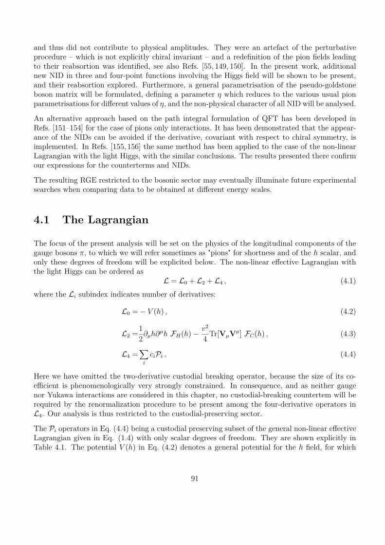
and thus did not contribute to physical amplitudes. They were an artefact of the perturbativeprocedure – which is not explicitly chiral invariant – and a redefinition of the pion fields leadingto their reabsortion was identified, see also Refs. [55, 149, 150]. In the present work, additionalnew NID in three and four-point functions involving the Higgs field will be shown to be present,and their reabsortion explored. Furthermore, a general parametrisation of the pseudo-goldstoneboson matrix will be formulated, defining a parameter ÷ which reduces to the various usual pionparametrisations for di�erent values of ÷, and the non-physical character of all NID will be analysed.

An alternative approach based on the path integral formulation of QFT has been developed inRefs. [151–154] for the case of pions only interactions. It has been demonstrated that the appear-ance of the NIDs can be avoided if the derivative, covariant with respect to chiral symmetry, isimplemented. In Refs. [155, 156] the same method has been applied to the case of the non-linearLagrangian with the light Higgs, with the similar conclusions. The results presented there confirmour expressions for the counterterms and NIDs.

The resulting RGE restricted to the bosonic sector may eventually illuminate future experimentalsearches when comparing data to be obtained at di�erent energy scales.

4.1 The Lagrangian

The focus of the present analysis will be set on the physics of the longitudinal components of thegauge bosons fi, to which we will refer sometimes as "pions" for shortness and of the h scalar, andonly these degrees of freedom will be explicited below. The non-linear e�ective Lagrangian withthe light Higgs can be ordered as

L = L0 + L2 + L4 , (4.1)where the Li subindex indicates number of derivatives:

L0 = ≠ V (h) , (4.2)

L2 =12ˆµhˆµh FH(h) ≠ v2

4 Tr[VµVµ] FC(h) , (4.3)

L4 =ÿ

i

ciPi . (4.4)

Here we have omitted the two-derivative custodial breaking operator, because the size of its co-e�cient is phenomenologically very strongly constrained. In consequence, and as neither gaugenor Yukawa interactions are considered in this chapter, no custodial-breaking countertem will berequired by the renormalization procedure to be present among the four-derivative operators inL4. Our analysis is thus restricted to the custodial-preserving sector.

The Pi operators in Eq. (4.4) being a custodial preserving subset of the general non-linear e�ectiveLagrangian given in Eq. (1.4) with only scalar degrees of freedom. They are shown explicitly inTable 4.1. The potential V (h) in Eq. (4.2) denotes a general potential for the h field, for which

91

only up to terms quartic in h will be made explicit, with arbitrary coe�cients µi and ⁄,

V © µ31 h + 1

2m2hh2 + µ3

3! h3 + ⁄

4!h4 . (4.5)

The first term in V (h) is provisionally kept in order to cancel the tadpole amplitude at one loop;we will clarify this point in Sect. 4.2.1. As before, the Higgs field is assumed to be physical onewith ÈhÍ = 0.

The present analysis will only require up to four-field vertices, for which it su�ces to explicit theh dependence of the functions Fi(h) up to quadratic terms. FH,C(h) will be thus parametrised as

FH,C(h) © 1 + 2aH,Ch/v + bH,Ch2/v2 , (4.6)

while for all Pi(h) operators in Table 4.1 the corresponding functions will be defined as

ciFi(h) © ci + 2aih/v + bih2/v2 . (4.7)

A further comment on FH(h) may be useful: through a redefinition of the h field [87] it would bepossible to absorb it completely. Nevertheless, this redefinition would a�ect all other couplings inwhich h participates and induce for instance corrections on fermionic couplings which are weightedby SM Yukawa couplings; it is thus pertinent not to disregard FH(h) here, as otherwise consistencywould require to include in the analysis the corresponding Fi(h) fermionic and gauge functions.If a complete basis including all SM fields is considered assigning individual arbitrary functionsFi(h) to all operators, it would then be possible to redefine away completely one Fi(h) withoutloss of generality: it is up to the practitioner to decide which set of independent operators he/shemay prefer, and to redefine away one of the functions, for instance FH(h). For the time being, wekeep explicit FH(h) all through, for the sake of generality 2.

We analyse next the freedom in defining the U matrix and work with a general parametrizationtruncated up to some order in fi/v. On-shell quantities must be independent of the choice ofparametrisation for the U matrix they thh, while it will be shown below that all NID dependinstead on the specific parametrisation chosen. The NID in which the h particle participates willturn out to o�er a larger freedom to be redefined away than the pure pionic ones.

4.1.1 The Lagrangian in a general U parametrisation

The non-linear ‡ model can be written as [55]

LNL = 12DµfiDµfi = v2

4 Tr[ˆµUˆµU†] = 12Gij(fi2)ˆµfiiˆ

µfij , (4.8)

where Dµ is a derivative “covariant” under the non-linear chiral symmetry. In geometric language,Gij(fi2) can be interpreted as the metric of a 3-sphere in which the pions live, and the freedom

2Note that FH(h) is not expected to be generated from the most popular composite Higgs models, as the latterbreak explicitly the chiral symmetry only via a potential for h externally generated, while FH(h) would requirederivative sources of explicit breaking of the chiral symmetry. A similar comment could be applied to P�H .

92

of parametrisation is just a coordinate transformation (see Ref. [148] and references therein).Indeed, Weinberg has shown [55] that di�erent linear realizations of the chiral symmetry wouldlead to di�erent metrics, which turn out to correspond to di�erent U parametrisations; they are allequivalent with respect to the dynamics of the pion fields as the non-linear transformation inducedon them is unique, and they are connected via redefinitions of the pion fields. In order to illustratethis correspondence explicitly, let us define general X and Y functions as follows:

U © X(z) + i· · fi

vY (z), z = fi2/v2 . (4.9)

X(z) and Y (z) are related via the unitarity condition UU† = 1,

X(z) =Ò

1 ≠ zY (z)2 . (4.10)

The Gij metric can now be rewritten as

Gij(fi2) = Y (z)2”ij + 41X Õ(z)2 + zY Õ(z)2 + Y (z)Y Õ(z)

2 fiifij

v2 , (4.11)

where the primes indicate derivatives with respect the the z variable, and Y (0) = ±1 is requiredfor canonically normalized pion kinetic terms.

The Lagrangian in Eq. (4.8) is invariant under the transformation Y æ ≠Y , or equivalentlyfi æ ≠fi. It is easy to relate X and Y to the functions in Weinberg’s analysis of chiral symmetry 3.A Taylor expansion of U up to order fi2N+2 bears N free parameters. A priori the present analysisrequires to consider in L2 terms up to O(fi6), as the latter may contribute to 4-point functionsjoining two of its pion legs into a loop. Nevertheless, the latter results in null contributions formassless pions, and in practice it will su�ce to consider inside U up to terms cubic on the pionfields. We thus define a single parameter ÷ which encodes all the parametrisation dependence,

Y (z) © 1 + ÷ z + O(z2) , (4.12)

resulting in

U = 1 ≠ fi2

2v2 ≠3

÷ + 18

4fi4

v4 + i(fi· )v

A

1 + ÷fi2

v2

B

+ . . . (4.13)

Specific values of ÷ can be shown to correspond to di�erent parametrisations up to terms withfour pions, for instance:

• ÷ = 0 yields the square root parametrisation: U =Ò

1 ≠ fi2/v2 + i(fi· )/v ,

• ÷ = ≠1/6 yields the exponential one: U = exp(ifi · ·/v) .

The L2 Lagrangian can now be written in terms of pion fields. Using the Fi(h) expansions inEqs. (4.6) and (4.7) it results

L2 =12ˆµhˆµh

A

1 + 2aHh

v+ bH

h2

v2

B

(4.14)

3The f(fi2) function defined in Ref. [55] is related to X and Y simply by f(x) = X(x)/Y (x)

93

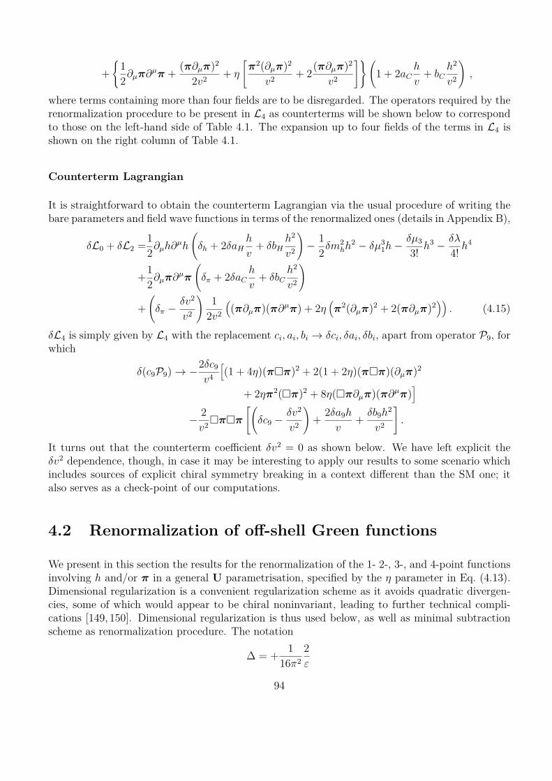
+I

12ˆµfiˆµfi + (fiˆµfi)2

2v2 + ÷

Cfi2(ˆµfi)2

v2 + 2(fiˆµfi)2

v2

DJ A

1 + 2aCh

v+ bC

h2

v2

B

,

where terms containing more than four fields are to be disregarded. The operators required by therenormalization procedure to be present in L4 as counterterms will be shown below to correspondto those on the left-hand side of Table 4.1. The expansion up to four fields of the terms in L4 isshown on the right column of Table 4.1.

Counterterm Lagrangian

It is straightforward to obtain the counterterm Lagrangian via the usual procedure of writing thebare parameters and field wave functions in terms of the renormalized ones (details in Appendix B),

”L0 + ”L2 =12ˆµhˆµh

A

”h + 2”aHh

v+ ”bH

h2

v2

B

≠ 12”m2

hh2 ≠ ”µ31h ≠ ”µ3

3! h3 ≠ ”⁄

4! h4

+12ˆµfiˆµfi

A

”fi + 2”aCh

v+ ”bC

h2

v2

B

+A

”fi ≠ ”v2

v2

B1

2v2

1(fiˆµfi)(fiˆµfi) + 2÷

1fi2(ˆµfi)2 + 2(fiˆµfi)2

22. (4.15)

”L4 is simply given by L4 with the replacement ci, ai, bi æ ”ci, ”ai, ”bi, apart from operator P9, forwhich

”(c9P9) æ ≠2”c9

v4

Ë(1 + 4÷)(fi⇤fi)2 + 2(1 + 2÷)(fi⇤fi)(ˆµfi)2

+ 2÷fi2(⇤fi)2 + 8÷(⇤fiˆµfi)(fiˆµfi)È

≠ 2v2⇤fi⇤fi

CA

”c9 ≠ ”v2

v2

B

+ 2”a9h

v+ ”b9h2

v2

D

.

It turns out that the counterterm coe�cient ”v2 = 0 as shown below. We have left explicit the”v2 dependence, though, in case it may be interesting to apply our results to some scenario whichincludes sources of explicit chiral symmetry breaking in a context di�erent than the SM one; italso serves as a check-point of our computations.

4.2 Renormalization of o�-shell Green functions

We present in this section the results for the renormalization of the 1- 2-, 3-, and 4-point functionsinvolving h and/or fi in a general U parametrisation, specified by the ÷ parameter in Eq. (4.13).Dimensional regularization is a convenient regularization scheme as it avoids quadratic divergen-cies, some of which would appear to be chiral noninvariant, leading to further technical compli-cations [149, 150]. Dimensional regularization is thus used below, as well as minimal subtractionscheme as renormalization procedure. The notation

� = + 116fi2

2Á

94

L4 operators Expansion in fi fields

c6P6 c6 [Tr(VµV µ)]2 F6(h)4c6

v4 (ˆµfiˆµfi)2

c7P7 c7Tr(VµV µ) 1v⇤h F7(h) ≠2c7

v3 ⇤h(ˆ‹fiˆ‹fi) ≠ 4a7

v4 (h⇤h)(ˆ‹fiˆ‹fi)

c8P8 c8Tr(VµV‹) 1v2 ˆµhˆ‹h F8(h) ≠2 c8

v4 (ˆµhˆ‹h)(ˆµfiˆ‹fi)

c9P9 c9Tr[(DµV µ)2] F9(h) ≠2c9

v4

Ëv2(⇤fi⇤fi)+2÷fi2(⇤fi)2+(1 + 4÷) (fi⇤fi)2

+8÷(fiˆµfi)(ˆµfi⇤fi) + (2 + 4÷) (ˆµfi)2(fi⇤fi)È

≠4a9

v3 h(⇤fi⇤fi) ≠ 2b9

v4 h2(⇤fi⇤fi)

c10P10 c10Tr(V‹DµV µ) 1v ˆ‹h F10(h)

≠2c10

v3 ˆ‹h(ˆ‹fi⇤fi) + ≠4a10

v4 hˆ‹h(ˆ‹fi⇤fi)

c11P11 c11 [Tr(VµV‹)]2 F11(h)4c11

v4 (ˆµfiˆ‹fi)2

c20P20 c20Tr(VµV µ) 1v2 ˆ‹hˆ‹h F20(h) ≠2c20

v4 (ˆµhˆµh)(ˆ‹fiˆ‹fi)

c⇤HP⇤H1v2 (⇤h⇤h) F⇤H(h)

c⇤H

v2 (⇤h⇤h) + 2a⇤H

v3 h (⇤h⇤h) + b⇤H

v4 h2 (⇤h⇤h)

c�HP�H1v3 (ˆµhˆµh)⇤h F�H(h)

c�H

v3 (ˆµhˆµh)⇤h + 2a�H

v4 (ˆµhˆµh)h⇤h

cDHPDH1v4 (ˆµhˆµh)2 FDH(h)

cDH

v4 (ˆµhˆµh)2

Table 4.1: The two columns on the left show the operators required to be in L4, Eq. (4.4), bythe renormalization procedure. The right hand side gives the corresponding explicit expansionin terms of pion and h fields (up to four fields), following the U expansion in Eq. (4.13) andthe Fi(h) parametrisation in Eq. (4.7).

95

Amplitudes2h 3h 4h 2fi 2fih 2fi2h 4fi

P6 c6P7 c7 a7P8 c8P9 c9 a9 b9 c9P10 c10 a10P11 c11P20 c20P⇤H c⇤H a⇤H b⇤H

P�H c�H a�H

PDH cDH

Table 4.2: Illustration of which operators in L4 (see Eq. (4.4) and Table 4.1) contribute to 2-,3-, and 4-point amplitudes involving pions and/or h fields. The specific operator coe�cientscontributing to each amplitude are indicated, following the ciFi expansion in Eq. (4.7).

will be adopted, while FeynRules, FeynArts, and FormCalc [157–161] will be used to compute one-loop amplitudes. Diagrams with closed pion loops give zero contribution for the case of masslesspions under study, and any reference to them will be omitted below.

Table 4.2 provides and overview of which L4 operator coe�cients contribute to amplitudes in-volving pions and/or h, up to 4-point vertices. It also serves as an advance over the results: alloperators in (4.4) will be shown to be required by the renormalization procedure. Furthermorewe have checked that they are all independent and thus their ensemble, when considered by itself,constitutes a complete and independent basis of scalar operators, up to four-derivatives in thenon-linear expansion. None of them should be disregarded on arguments of their tradability forother operators, for instance for fermionic ones via the application of the equations of motion(EOM), unless the latter operators are explicitly included as part of the analysis, or without fur-ther assumptions (i.e. to neglect all fermion masses). See Sect. 4.4 for comparison with previousliterature.

4.2.1 1-point functions

Because of chiral symmetry pions always come in even numbers in any vertex, unlike Higgs parti-cles, thus tadpole contributions may be generated only for the latter. At tree-level it would su�ceto set µ1 = 0 in V (h) (Eq. (4.2)) in order to insure ÈhÍ = 0. At one-loop, a tadpole term is inducedfrom the triple Higgs couplings µ3 and aH , though, via the Feynman diagram in Fig. 4.1. Thecounterterm required to cancel this contribution reads

”µ31 = m2

h

A

µ3 ≠ 4aHm2

h

v

B

�Á , (4.16)

and has no impact on the rest of the Lagrangian.

96

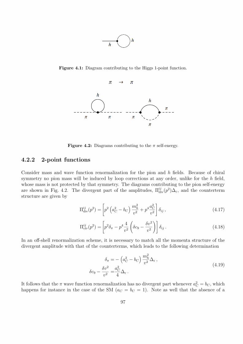
Figure 4.1: Diagram contributing to the Higgs 1-point function.

Figure 4.2: Diagrams contributing to the fi self-energy.


Consider mass and wave function renormalization for the pion and h fields. Because of chiralsymmetry no pion mass will be induced by loop corrections at any order, unlike for the h field,whose mass is not protected by that symmetry. The diagrams contributing to the pion self-energyare shown in Fig. 4.2. The divergent part of the amplitudes, �ij

div(p2)�Á, and the countertermstructure are given by

�ijdiv(p2) =

C

p21a2

C ≠ bC

2 m2h

v2 + p4 a2C

v2

D

”ij , (4.17)

�ijctr(p2) =

C

p2”fi ≠ p4 4v2

A

”c9 ≠ ”v2

v2

BD

”ij . (4.18)

In an o�-shell renormalization scheme, it is necessary to match all the momenta structure of thedivergent amplitude with that of the counterterms, which leads to the following determination

”fi = ≠1a2

C ≠ bC

2 m2h

v2 �Á ,

”c9 ≠ ”v2

v2 =a2C

4 �Á .

(4.19)

It follows that the fi wave function renormalization has no divergent part whenever a2C = bC , which

happens for instance in the case of the SM (aC = bC = 1). Note as well that the absence of a

97

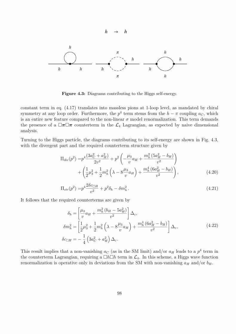
Figure 4.3: Diagrams contributing to the Higgs self-energy.

constant term in eq. (4.17) translates into massless pions at 1-loop level, as mandated by chiralsymmetry at any loop order. Furthermore, the p4 term stems from the h ≠ fi coupling aC , whichis an entire new feature compared to the non-linear ‡ model renormalization. This term demandsthe presence of a ⇤fi⇤fi counterterm in the L4 Lagrangian, as expected by naive dimensionalanalysis.

Turning to the Higgs particle, the diagrams contributing to its self-energy are shown in Fig. 4.3,with the divergent part and the required counterterm structure given by

�div(p2) =p4 (3a2C + a2

H)2v2 + p2

A

≠µ3

vaH + m2

h (5a2H ≠ bH)v2

B

+A

12µ2

3 + 12m2

h

3⁄ ≠ 8µ3

vaH

4+ m4

h (6a2H ≠ bH)v2

B

, (4.20)

�ctr(p2) =p4 2”c⇤H

v2 + p2”h ≠ ”m2h . (4.21)

It follows that the required counterterms are given by

”h =C

µ3

vaH + m2

h (bH ≠ 5a2H)

v2

D

�Á,

”m2h =

C12µ2

3 + 12m2

h

3⁄ ≠ 8µ3

vaH

4+ m4

h (6a2H ≠ bH)v2

D

�Á,

”c⇤H = ≠ 14

13a2

C + a2H

2�Á.

(4.22)

This result implies that a non-vanishing aC (as in the SM limit) and/or aH leads to a p4 term inthe counterterm Lagrangian, requiring a ⇤h⇤h term in L4. In this scheme, a Higgs wave functionrenormalization is operative only in deviations from the SM with non-vanishing aH and/or bH .

98

Figure 4.4: Diagrams contributing to the hh æ h amplitude, not including diagrams ob-tained by crossing.


The calculational details for the 3- and 4-point functions will not be explicitly shown as they arenot particularly illuminating. See Appendix B for more details. Vertices with an odd number oflegs necessarily involve at least one Higgs particle.

hhh

Let us consider first the hhh amplitude at one loop. The relevant diagrams to be computed aredisplayed in Fig. 4.4. As h behaves as a generic singlet, the vertices involving uniquely externalh legs which appear in the Lagrangian Eq. (4.1) will span all possible momentum structures thatcan result from one-loop amplitudes. Hence any divergence emerging on amplitudes involving onlyexternal h particles will be easily absorbable. The specific results for the counterterms emergingfrom L0 and L2 can be found in Appendix B.

fifih

The diagrams for fifih amplitudes are shown in Fig. 4.5. The one-loop divergences are studiedin detail in Appendix B; for instance, it turns out that neither ”aC nor ”a9 are induced in theSM limit. Chiral symmetry restricts the possible structures spanned by the pure fi and h ≠ fioperators. Because of this, it turns out that part of the divergent amplitude induced by the lastdiagram in Fig. 4.5 cannot be cast as a function of the L2 and L4 operators, that is, it cannot bereabsorbed by chiral-invariant counterterms, and furthermore its coe�cient depends on the pionparametrisation used: an apparent non chiral-invariant divergence (NID) has been identified. NIDsare an artefact of the apparent breaking of chiral symmetry when the one-loop analysis is treatedin perturbation theory [55] and have no physical impact as they vanish for on-shell amplitudes.While long ago NIDs had been isolated in perturbative analysis of four-pion vertices in the non-linear sigma model [148], the result obtained here is a new type of NID: a three-point function

99

Figure 4.5: Diagrams contributing to the fifi æ h scattering amplitude, not includingdiagrams obtained by crossing.

involving the Higgs particle, corresponding to the chiral non-invariant operator

ONID1 = ≠aC

332 + 5÷

4 �Á

v3 fi⇤fi⇤h . (4.23)

This coupling cannot be reabsorbed as part of a chiral invariant counterterm, but its contributionto on-shell amplitudes indeed vanishes. It is interesting to note that while the renormalizationconditions of all physical parameters turn out to be independent of the choice of U parametrisation,as they should, NIDs exhibit instead an explicit ÷ dependence, as illustrated by Eq. (4.23). Thispattern will be also present in the renormalization of 4-point functions, developed next.


The analysis of this set of correlation functions turns out to be tantalizing when comparing theresults for mixed fi ≠ h vertices with those for pure pionic ones 4.

fifihh

The computation of the fifi æ hh one-loop amplitude shows that the renormalization procedurerequires the presence of all possible chiral invariant hhfifi counterterms in the Lagrangian, in themost general case.

4It provides in addition nice checks of the computations; for instance we checked explicitly in the present contextthat the consistency of the renormalization results for four-point functions requires ”2

v = 0.

100

Furthermore, we have identified new NIDs in hhfifi amplitudes:

ONID2 = +(2a2

C ≠ bC)33

2 + 5÷4 �Á

v4 fi⇤fi h⇤h ,

ONID3 = +(a2

C ≠ bC)33

2 + 5÷4 �Á

v4 fi⇤fi ˆµhˆµh ,

ONID4 = ≠2a2

C

332 + 5÷

4 �Á

v4 fiˆµfi ˆµh⇤h .

(4.24)

While these NIDs di�er from that for the three-point function in Eq. (4.23) in their countertermstructure, they all share an intriguing fact: to be proportional to the factor (3/2 + 5÷). Thereforea proper choice of parametrisation, i.e. ÷ = ≠3/10, removes all mixed h ≠ fi NIDs. That value of÷ is of no special significance as fas as we know, and in fact there is no choice of parametrisationthat can avoid all noninvariant divergencies, as proved next.

fifififi

Consider now fifi æ fifi amplitudes. Only two counterterms are necessary to reabsorb chiral-invariant divergencies, namely ”c6 and ”c11. In this case, we find no other NIDs than those alreadypresent in the non-linear ‡ model [148], which stemmed from the insertion in the loop of thefour-pion vertex (whose coupling depends on ÷). Our analysis shows that the four-fi NIDs read:

ONID5 = +

39÷2 + 5÷ + 3

4

4 �Á

v4 (fi⇤fi)2,

ONID6 = +

51 + 4÷ +

312 + ÷

4a2

C

6 �Á

v4 (fi⇤fi)(ˆµfiˆµfi),

ONID7 = +2÷2 �Á

v4 fi2(⇤fi)2,

ONID8 = +2÷

1a2

C ≠ 12 �Á

v4 (⇤fiˆµfi)(fiˆµfi).

(4.25)

As expected, the parametrisation freedom – the dependence on the ÷ parameter – appears onlyin NIDs, and never on chiral-invariant counterterms, as the latter describe physical processes.Furthermore, the contribution of all NIDs to on-shell amplitudes vanishes as expected 5. Finally,the consideration of the ensemble of three and four-point NIDs in Eqs. (4.23), (4.24) and (4.25)shows inmediately that no parametrisation can remove all NIDs: it is possible to eliminate thoseinvolving h 6, but no value of ÷ would remove all pure pionic ones.

hhhh

The renormalization procedure for hh æ hh amplitudes is straightforward. It results in contri-butions to ”a�H , ”cDH , and ”bH . Interestingly, Appendix C illustrates that large coe�cients are

5This is not always seen when taken individually. For instance, the contribution of ONID4 to the hhfifi amplitude

is cancelled by that of ONID1 , which corrects the hfifi vertex.

6This may be linked to the larger freedom of redefinition for fields not subject to chiral invariance.

101

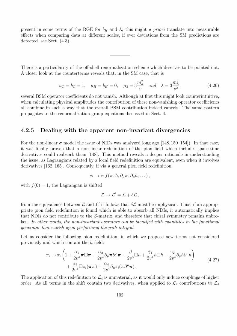
present in some terms of the RGE for bH and ⁄; this might a priori translate into measurablee�ects when comparing data at di�erent scales, if ever deviations from the SM predictions aredetected, see Sect. (4.3).

There is a particularity of the o�-shell renormalization scheme which deserves to be pointed out.A closer look at the counterterms reveals that, in the SM case, that is

aC = bC = 1, aH = bH = 0, µ3 = 3m2h

vand ⁄ = 3m2

h

v2 , (4.26)

several BSM operator coe�cients do not vanish. Although at first this might look counterintuitive,when calculating physical amplitudes the contribution of these non-vanishing operator coe�cientsall combine in such a way that the overall BSM contribution indeed cancels. The same patternpropagates to the renormalization group equations discussed in Sect. 4.

4.2.5 Dealing with the apparent non-invariant divergencies

For the non-linear ‡ model the issue of NIDs was analyzed long ago [148,150–154]). In that case,it was finally proven that a non-linear redefinition of the pion field which includes space-timederivatives could reabsorb them [148]. This method reveals a deeper rationale in understandingthe issue, as Lagrangians related by a local field redefinition are equivalent, even when it involvesderivatives [162–165]. Consequently, if via a general pion field redefinition

fi æ fi f(fi, h, ˆµfi, ˆµh, . . . ) ,

with f(0) = 1, the Lagrangian is shifted

L æ LÕ = L + ”L ,

from the equivalence between L and LÕ it follows that ”L must be unphysical. Thus, if an approp-priate pion field redefinition is found which is able to absorb all NDIs, it automatically impliesthat NDIs do not contribute to the S-matrix, and therefore that chiral symmetry remains unbro-ken. In other words, the non-invariant operators can be identifed with quantities in the functionalgenerator that vanish upon performing the path integral.

Let us consider the following pion redefinition, in which we propose new terms not consideredpreviously and which contain the h field:

fii æ fii

A

1 + –1

2v4 fi⇤fi + –2

2v4 ˆµfiˆµfi + —

2v3⇤h + “1

2v4 h⇤h + “2

2v4 ˆµhˆµh

B

+ –3

2v4⇤fii(fifi) + –4

2v4 ˆµfii(fiˆµfi).(4.27)

The application of this redefinition to L4 is immaterial, as it would only induce couplings of higherorder. As all terms in the shift contain two derivatives, when applied to L2 contributions to L4

102

and NID operator coe�cients do follow. Indeed, the action of Eq. (4.27) on L2 reduces to that onthe term

14Tr(ˆµUˆµU)FC(h) , (4.28)

which produces the additional contribution to NDI vertices given by

�LNID = ≠fi⇤fi

A–1

v4 fi⇤fi + –2

v4 ˆµfiˆµfi + —

v3⇤h + “1

v4 h⇤h + “2

v4 ˆµhˆµh

B

≠ –3

v4 (⇤fi⇤fi)(fifi) ≠ –4

v4 (⇤fiˆµfi)(fiˆµfi) ≠ 2aC—

v4 fiˆµfiˆµh⇤h + ... (4.29)

where “1 = 2aC— + “1, and where the dots indicate other operators with either six derivatives orthat have more than four fields and are beyond the scope of this work. Comparing the terms in�LNID with the NID operators found, Eqs. (4.23), (4.24) and (4.25), it follows that by choosing

–1 =3

9÷2 + 5÷ + 34

4�Á,

–2 =51 + 4÷ +

312 + ÷

4a2

C

6�Á,

–3 = 2÷2�Á,

–4 = 2÷1a2

C ≠ 12

�Á,

— = ≠33

2 + 5÷4

aC�Á,

“1 =33

2 + 5÷4 1

2a2C ≠ bC

2�Á,

“2 =33

2 + 5÷4 1

a2C ≠ bC

2�Á.

all 1-loop NID are removed away.

A few comments are in order. The o�-shell renormalization of one loop amplitudes is delicateand physically interesting. Because of chiral symmetry, the pure pionic or mixed pion-h operatorsdo not encode all possible momentum structures, even after pion field redefinitions. Hence, theappearance of divergent structures that can be absorbed by ”L0, ”L2, ”L4 and �LNI is a man-isfestation of chiral invariance and of the field redefinition equivalence discussed above. We haveshown consistently that NIDs appearing in the one-loop renormalization of the electroweak chiralLagrangian do not contribute to on-shell quantities. In fact, a closer examination has revealedthat the apparent chiral non-invariant divergencies emerge from loop diagrams which have at leastone four-pion vertex in it, and this is why all of them depend on ÷. We have also shown that thepresence of a light Higgs boson modifies the coe�cients of the unphysical counterterms made outpurely of pions, but not their structure, neither -of course- breaks chiral symmetry.

4.3 Renormalization Group Equations

It is straightforward to derive the RGE from the ”ci divergent contributions determined in theprevious section. The complete RGE set can be found in Appendix C. As illustration, the evolutionof those Lagrangian coe�cients which do not vanish in the SM limit is given by:

16fi2 d

d ln µaC = aC

C15a2

H ≠ 3bC ≠ bH

2 m2h

v2 ≠ aHµ3

v

D

103

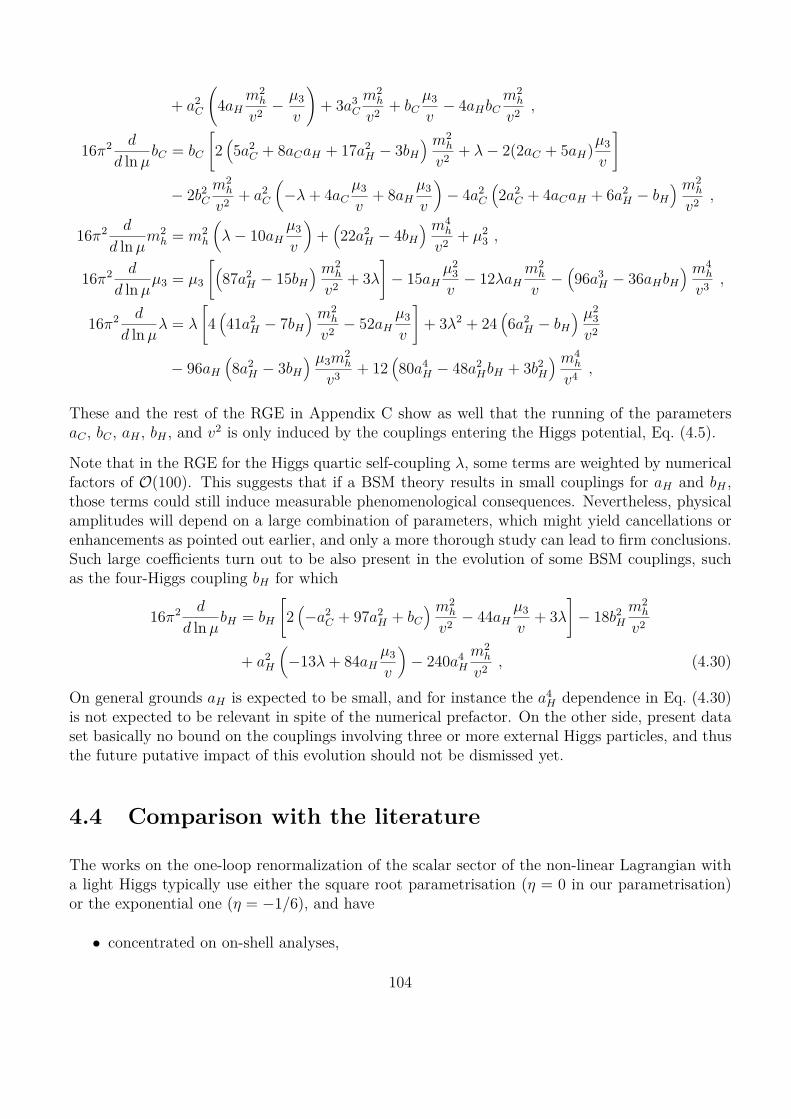
+ a2C

A

4aHm2

h

v2 ≠ µ3

v

B

+ 3a3C

m2h

v2 + bCµ3

v≠ 4aHbC

m2h

v2 ,

16fi2 d

d ln µbC = bC

C

215a2

C + 8aCaH + 17a2H ≠ 3bH

2 m2h

v2 + ⁄ ≠ 2(2aC + 5aH)µ3

v

D

≠ 2b2C

m2h

v2 + a2C

3≠⁄ + 4aC

µ3

v+ 8aH

µ3

v

4≠ 4a2

C

12a2

C + 4aCaH + 6a2H ≠ bH

2 m2h

v2 ,

16fi2 d

d ln µm2

h = m2h

3⁄ ≠ 10aH

µ3

v

4+

122a2

H ≠ 4bH

2 m4h

v2 + µ23 ,

16fi2 d

d ln µµ3 = µ3

C187a2

H ≠ 15bH

2 m2h

v2 + 3⁄

D

≠ 15aHµ2

3v

≠ 12⁄aHm2

h

v≠

196a3

H ≠ 36aHbH

2 m4h

v3 ,

16fi2 d

d ln µ⁄ = ⁄

C

4141a2

H ≠ 7bH

2 m2h

v2 ≠ 52aHµ3

v

D

+ 3⁄2 + 2416a2

H ≠ bH

2 µ23

v2

≠ 96aH

18a2

H ≠ 3bH

2 µ3m2h

v3 + 12180a4

H ≠ 48a2HbH + 3b2

H

2 m4h

v4 ,

These and the rest of the RGE in Appendix C show as well that the running of the parametersaC , bC , aH , bH , and v2 is only induced by the couplings entering the Higgs potential, Eq. (4.5).

Note that in the RGE for the Higgs quartic self-coupling ⁄, some terms are weighted by numericalfactors of O(100). This suggests that if a BSM theory results in small couplings for aH and bH ,those terms could still induce measurable phenomenological consequences. Nevertheless, physicalamplitudes will depend on a large combination of parameters, which might yield cancellations orenhancements as pointed out earlier, and only a more thorough study can lead to firm conclusions.Such large coe�cients turn out to be also present in the evolution of some BSM couplings, suchas the four-Higgs coupling bH for which

16fi2 d

d ln µbH = bH

C

21≠a2

C + 97a2H + bC

2 m2h

v2 ≠ 44aHµ3

v+ 3⁄

D

≠ 18b2H

m2h

v2

+ a2H

3≠13⁄ + 84aH

µ3

v

4≠ 240a4

H

m2h

v2 , (4.30)

On general grounds aH is expected to be small, and for instance the a4H dependence in Eq. (4.30)

is not expected to be relevant in spite of the numerical prefactor. On the other side, present dataset basically no bound on the couplings involving three or more external Higgs particles, and thusthe future putative impact of this evolution should not be dismissed yet.

4.4 Comparison with the literature

The works on the one-loop renormalization of the scalar sector of the non-linear Lagrangian witha light Higgs typically use either the square root parametrisation (÷ = 0 in our parametrisation)or the exponential one (÷ = ≠1/6), and have

• concentrated on on-shell analyses,

104

• disregarded the impact of FH(h),

• disregarded fermionic operators; in practice this means to neglect all fermion masses.

This last point is not uncorrelated with the fact that the basis of independent four-derivativeoperators determined here has a larger number of elements than previous works about the scalarsector. Those extra bosonic operators have been shown here to be required by the countertermprocedure. It is possible to demonstrate, though, that they can be traded via EOM by othertype of operators including gauge corrections and Yukawa-like operators. In a complete basisof all possible operators it is up to the practitioner to decide which set is kept, as long as itis complete and independent. When restricting instead to a given subsector, the complete andconsistent treatment requires to consider all independent operators of the kind selected (anywaythe renormalization procedure will indicate their need), or to state explicitly any extra assumptionsto eliminate them. Some further specific comments:

Ref. [143] considers, under the first two itemized conditions above plus disregarding the impact ofV (h) (and in particular neglecting the Higgs mass), the scattering processes hh æ hh, fifi æ hhand fifi æ fifi. With the o�-shell treatment, five additional operators result in this case withrespect to those obtained in that reference (assuming the rest of their assumptions), P7, P9, P10,P⇤H and P�H in Table 4.1. Note that all these operators contain either ⇤h or ⇤fi inside; theymay thus be implicitly traded by fermionic operators via EOM, and can only be disregarded ifall fermion masses are neglected. Assuming this extra condition, we could reproduce their resultsusing the EOMs. For instance, the RGEs derived here for c6, c8, c20, aC and bC di�er from thecorresponding ones in that reference: an o�-shell renormalization analysis entails the larger numberof operators mentioned. In any case, we stress again that the results of both approaches coincidewhen calculating physical amplitudes. Another contrast appears in the running of aC , bC , aH , bH ,as well as the mass, the triple, and the quartic coupling of the Higgs, for which the running isinduced by the Higgs potential parameters, disregarded in that reference.

In Ref. [144] the on-shell scattering process of the longitudinal modes of the process W +W ≠ æ ZZis considered, disregarding FH(h) but including the impact of V (h). Our o�-shell treatment resultsin this case in one additional operator (assuming the rest of their assumptions) with respect tothose in that reference, P9, as only processes involving four goldstone bosons were consideredthere. Again this extra operator contains ⇤fi in all its terms and it could be neglected in practiceif disregarding all fermion masses. With this extra assumption, our results reduce to theirs in thelimit indicated.

Finally, in Refs. [155, 156] the geometrical formulation of HEFT has been adopted. It has beendemonstrated that quantum corrections to the theory are given in terms of the curvature andconnection of the scalar manifold. In particular it has been shown that the NIDs appear due tononcovariant term in the second variation of action which is explicitly proportional to EOM andcan be eliminated if the variation is promoted to be covariant with respect to the chiral symmetryof the Lagrangian (see Eq.7 in Ref. [156]). The expressions for NID match exactly the resultspresented in this Chapter.

105

Summary

Completely clarifying the mechanism of the electroweak breaking is one of the main goals ofparticle physics today and an important role, on the theory side, is played by simple and motivatedextensions of the SM which could provide guidance in the experimental search.

To this purpose we have formulated a model where the scalar sector of the SM is minimallyextended to include an additional scalar particle ‡, singlet under the SM gauge group. To alarge extent our set up is motivated by the QCD linear sigma model. Similarly, we consider alinear realization of symmetry, where the Higgs fourplet together the ‡ scalar forms a fundamentalrepresentation of SO(5) global symmetry, broken down spontaneously to SO(4). This minimalSO(5)/SO(4) coset includes four GB states, three of which are to become longitudinal polarisationsof W and Z bosons as in the SM itself and one additional state is the observed Higgs particle. Inorder to reproduce the observed Higgs mass an explicit breaking of the global SO(5) symmetryis needed. To introduce it we consider the extended fermionic sector in complete representationsof SO(5) group, linearly coupled to the SM fermions through SO(5) violating couplings. Proto-Yukawa interactions between the scalar 5plet and the new fermions allow for the explicit breakingto propagate to the scalar potential due to Coleman-Weinberg mechanism and to generate apotential for the Higgs fourplet, which eventually triggers the EWSB.

The previous attempt in this direction [22] did not fully take into account the impact of theextended fermionic sector on the main phenomenological observables. Instead, we considered therestrictions set on the parameter space of the fermionic sector by EWPT parameters, namely S, Tand Rb. Concerning the scalar contribution, from an explicit one-loop computation we recover awell-known result: a positive contribution to the S parameter and a negative contribution to theT parameter. In our model both extra contributions �S and �T are finite, so there is no cut-o�ambiguity. The main impact of the heavy fermion contribution is on the T parameter. Lettingthe heavy fermions to be as light as 800 GeV, the lower limit from direct searches, contributionsto T of both signs as large as 0.2. Even the largest scalar contributions to �S and �T , obtainedwhen the scalars mixing angle “ saturates its experimental bound and ‡ is very heavy, can alwaysbe compensated by the fermionic ones for an appropriate choice of the parameters, keeping S andT within the experimentally allowed region. Thus, we conclude that large part of the parameterspace is allowed by EWPT and therefore the theory is fully viable.

The direct LHC searches for a scalar particle together with the theoretical requirement that theHiggs behaves as a pseudo-Goldstone boson, allow to exclude ‡ masses below about 500 GeV.

Furthermore, we have integrated out the BSM states and obtained the e�ective Lagrangian. First,

106

linear e�ective Lagrangian has been derived by integration out of the heavy fermionic states. ThisLagrangian describes interactions of the Higgs and ‡ scalars with the SM fermionic matter. As asecond step we introduce the e�ective Yukawa operator, characterized by two parameters, whichdepend only on the embeddings of the fermions into SO(5) representations . Having this, wehave derived the benchmark non-linear e�ective Lagrangian for the large mass limit of the heavyscalar ‡. Up to the first order in the linear corrections it contains ten operators, five bosonic andfive fermionic. The coe�cients of the latter ones are given as functions of the two parametersof Yukawa interaction, thus allowing for a simple comparison between the models with variousembeddings adopted.

We have derived for the first time ‡ induced modifications of the Higgs to gauge bosons andfermions couplings ŸV and Ÿf and shown that they are quite universal. While the leading ordercorrections, obtained in the limit of the infinite scalar mass coincide with the ones previouslyobtained in the literature, the new next to leading corrections are doubly suppressed by smallexplicit breaking parameters and large scalar self coupling, a combination corresponding to am2

h/m2s suppression. We have repeated the integration out procedure for the UV complete model

considered previously and identified the coe�cients of the e�ective operators in terms of theparameters of extended fermionic sector as well as scalar sector with the ‡ boson. The resultingoperators represent a subset of the most general non-linear Lagrangian and are consistent with theresults for the general SO(5)/SO(4) constructions given in [70].

Next, we have performed the one-loop o�-shell renormalization of the custodial-preserving sectorof e�ective non-linear Lagrangian with the finite Higgs mass, focusing on its scalar sector composedof longitudinal components of the SM gauge bosons and the Higgs boson h. We have identifiedthe NLO counterterms required to absorb the divergences originating from the diagrams with upto 4 external legs, in the agreement with the NDA the general non-linear Lagrangian.

As a useful tool we introduce a novel general parametrisation of the Goldstone boson matrix, at theorder considered depending on single parameter ÷. All the counterterms induced are parametri-sation independent. We have also found chrial noninvariant divergences, which depend explicitlyon ÷ and generalize the result of [148] to the case of the light Higgs present in the spectrum. Wedemonstrated how they can be removed by the pion field redefinition, thus being unphysical andvanishing on-shell. Our findings have been later confirmed by an independent group [155, 156],where the same non-invariant divergences have been found, it has also been shown that they canbe avoided by employing of covariant variation of the action in the path integral approach to therenormalization.

To sum up the above we have constructed the viable UV complete model of Goldstone Higgs whichis possible to validate by the ongoing LHC run either through direct observation of the heavy scalar‡ and/or heavy fermionic partners of the SM fermions. At low energies, below the masses of BSMparticles the model results in the set of non-linear operators parametrizing the deviations fromthe SM predictions with the coe�cients being the explicit functions of the parameters of the UVcompletion. We have analysed the consistency of the subset of non-linear Lagrangian by analysingits one loop structure in general U parametrisation and confirmed the previous results based onNDA.

107

Acknowledgements

First of all I would like to mention my supervisor back in Russia, Grigory Moiseevich Vereshkov,without whom my scientific journey would not be possible, rest in peace. Next, I would like tothank Gruppo 4 of INFN Padova and Padova University for hosting me all these years and theprofessors I collaborated with in Padova and Madrid, namely Stefano Rigolin, Ferruccio Feruglioand Belen Gavela for the discussions and inspiring ideas. I have appreciated a lot working (a lot)with Sara Saa, Pedro Machado and Rodrigo Alonso with whom much time was spent hunting formissing minus signs and factors of 2, I believe we caught them all eventually. One more personworth noting, spasibo to Oleksii Matsedonskyi, who graduated from here 3 years ago, for beingmy friend and from whom I learned quite a bit. It was really a great experience to be a partof the Invisibles crew, where I have met many amazing people who became my friends, specialregards go to Thomas Neder and Ignacio Hierro. I also hope that the tradition of the Russiandinners, started my Michele Lucente (not by me!) at the Invisibles conferences will continue. Iwould also like to mention all the people who cheered me up at my hard times and who supportedme. Thanks to my parents for believing in me even without clear understanding of what I amdoing (and where). Muchas gracias to Belen Gavela for giving me the opportunity to discoverthe world and to make great science with great people, herself included. Finally, I thank StefanoRigolin and Ignacio Hierro for correcting the thesis, I felt your pain, and quoting Marija Kekic:“No way we are going to put articles correctly”. Finally thanks my ex-o�cemate Giacomo Bighinfor translating the abstract of the thesis to Italian and apart from this being a great o�cematetogether with Jagjit Singh!

108

Appendix A

Coleman–Weinberg Potential

In Sect. 2.1 it was assumed a specific form for the SO(5) scalar potential broken to SO(4), in-troducing two additional SO(5) breaking parameters – and —. Here we will further motivate thisassumption. Even assuming that the tree level scalar potential would preserve the global SO(5)symmetry, the presence of a SO(5) breaking couplings in the fermionic sector will generate at one-loop level SO(5) breaking terms through the Coleman-Weinberg mechanism [71]. The one-loopfermionic contribution can be obtained from the field dependent mass matrix M as

Vloop = ≠ i

2

⁄ d4k

(2fi)4

Œÿ

n=1

1n

TrA

MM†

k2

Bn

= i

2

⁄ d4k

(2fi)4 Tr logA

1 ≠ MM†

k2

B

= ≠ 164fi2

A

�2TrËMM†

È≠ Tr

Ë(MM†)2

Èlog

A�2

µ2

B

+

+TrC

(MM†)2 logA

MM†

µ2

BD

≠ 12Tr

Ë(MM†)2

ÈB

, (A.1)

where � is the UV cuto� scale while µ is a generic renormalization scale. The first two terms onthe right-hand side of this equation are divergent, respectively quadratically and logarithmically,while the last two terms are finite. For the model under discussion it results:

Tr[MM†] = c1 + c2 („T „) , (A.2)Tr[(MM†)2] = d1 + d2 ‡ + d3 ‡2 + d4 („T „) + d5 („T „)2 , (A.3)

where

c1 = 2�21 + �2

2 + �23 + M2

1 + 5 M25 + ({} ¡ {}Õ) ,

c2 = y21 + y2

2 + ({} ¡ {}Õ) ,

and

d1 = M41 + 5M4

5 + 2M25

12�2

1 + �22

2+ 2M2

1 �23 + 2�4

1 +1�2

2 + �23

22+ ({} ¡ {}Õ) ,

d2 = 4 (y1M1 + y2M5) �2�3 + ({} ¡ {}Õ) ,

109

d3 = 2 y21�2

2 ≠ y22�2

1 + ({} ¡ {}Õ) ,

d4 = 4 y1y2M1M5 + 21y2

1 + y22

2 1M2

1 + M25

2+ y2

2

1�2

1 + 2�23

2+ ({} ¡ {}Õ) ,

d5 = y41 + y4

2 + ({} ¡ {}Õ) .

In consequence, only the quadratically divergent piece is seen to remain SO(5) invariant, while therest of the potential introduces an explicit breaking of the SO(5) symmetry to SO(4), see Eq. (A.3).The quadratic divergence can be thus absorbed in the parameters of the tree-level Lagrangian, andthe same holds for the SO(5) invariant component of the logarithmically divergent terms (d1, d4and d5). However, the presence of the d2 and d3 divergent SO(5)-breaking terms require to addthe two corresponding counterterms in the potential, so as to obtain a renormalizable theory.These two necessary terms are those defined with coe�cients – and — in the potential definitionEq. (2.8). The gauge couplings appearing in the covariant derivatives also break explicitly theSO(5) symmetry, but they do not induce extra one-loop divergent contributions to the e�ectivepotential, and in consequence only – and — are required for consistency.

The computation of the finite part of Vloop should provide the dependence of the parameters on therenormalization scale 1 and should thus be equivalent to the computation of their renormalizationgroup equations; this task is beyond the scope of the present analysis.

1The gauge bosons induce finite contributions which are usually neglected with respect to the fermionic ones,as their relative ratio is proportional to the ratio between the mass scale for the heavy fermions and that for thegauge bosons.

110

Appendix B

The counterterms

Details about the computation of the counterterms and the renormalization of the chiral La-grangian are given in this Appendix, including the derivation of the RGEs.

The bare parameters (denoted by b) written in terms of the renormalized ones and the countertermsfor the L2 and L4 Lagrangians are given by

hb =Ò

Zhh, ”h © Zh ≠ 1,

fib =Ò

Zfifi, ”fi © Zfi ≠ 1,

v2b = Zfi(v2 + ”v2)µ≠Á,

(m2h)b = 1

Zh(m2

h + ”m2h),

(µ31)b = 1

Z1/2h

1µ3

1 + ”µ31

2µ3Á/2,

µb3 = 1

Z3/2h

(µ3 + ”µ3) µÁ/2,

⁄b = 1Z2

h

(⁄ + ”⁄) µÁ,

abC = 1

Z1/2fi Z1/2

h

A

aC + ”aC + aC

2”v2

v2

B

,

bbC = 1

Zh

A

bC + ”bC + bC”v2

v2

B

,

abH = Z1/2

fi

Z3/2h

A

aH + ”aH + aH

2”v2

v2

B

,

bbH = Zfi

Z2h

A

bH + ”bH + bH”v2

v2

B

,

(B.1)

111

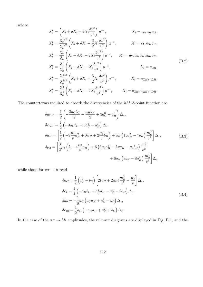
whereXb

i =A

Xi + ”Xi + 2Xi”v2

v2

B

µ≠Á, Xi = c6, c9, c11,

Xbi = Z1/2

fi

Z1/2h

A

Xi + ”Xi + 32Xi

”v2

v2

B

µ≠Á, Xi = c7, a9, c10,

Xbi = Zfi

Zh

A


v2

B

µ≠Á, Xi = a7, c8, b9, a10, c20,

Xbi = Zfi

Zh

A

Xi + ”Xi + Xi”v2

v2

B

µ≠Á, Xi = c⇤H ,

Xbi = Z3/2

fi

Z3/2h

A

Xi + ”Xi + 32Xi

”v2

v2

B

µ≠Á, Xi = a⇤H , c�H ,

Xbi = Z2

fi

Z2h

A


v2

B

µ≠Á, Xi = b⇤H , a�H , cDH .

(B.2)

The counterterms required to absorb the divergencies of the hhh 3-point function are

”a⇤H = 12

A

≠3aCbC

2 ≠ aHbH

2 + 3a3C + a3

H

B

�Á,

”c�H = 12

1≠3aCbC + 3a3

C ≠ a3H

2�Á,

”aH =C

12

3≠9µ3

va2

H + ⁄aH + 2µ3

vbH

4+ aH

115a2

H ≠ 7bH

2 m2h

v2

D

�Á,

”µ3 =C

32µ3

3⁄ ≠ 4µ3

vaH

4+ 6

16µ3a

2H ≠ ⁄vaH ≠ µ3bH

2 m2h

v2

+ 6aH

13bH ≠ 8a2

H

2 m4h

v3

D

�Á,

(B.3)

while those for fifi æ h read

”aC = 12

1a2

C ≠ bC

2 C

2(aC + 2aH)m2h

v2 ≠ µ3

v

D

�Á,

”c7 = 14

1≠aHbC + a2

CaH ≠ a3C ≠ 2aC

2�Á,

”a9 = ≠18aC

1aCaH + a2

C ≠ bC

2�Á,

”c10 = 12aC

1≠aCaH + a2

C + bC

2�Á.

(B.4)

In the case of the fifi æ hh amplitudes, the relevant diagrams are displayed in Fig. B.1, and the

112

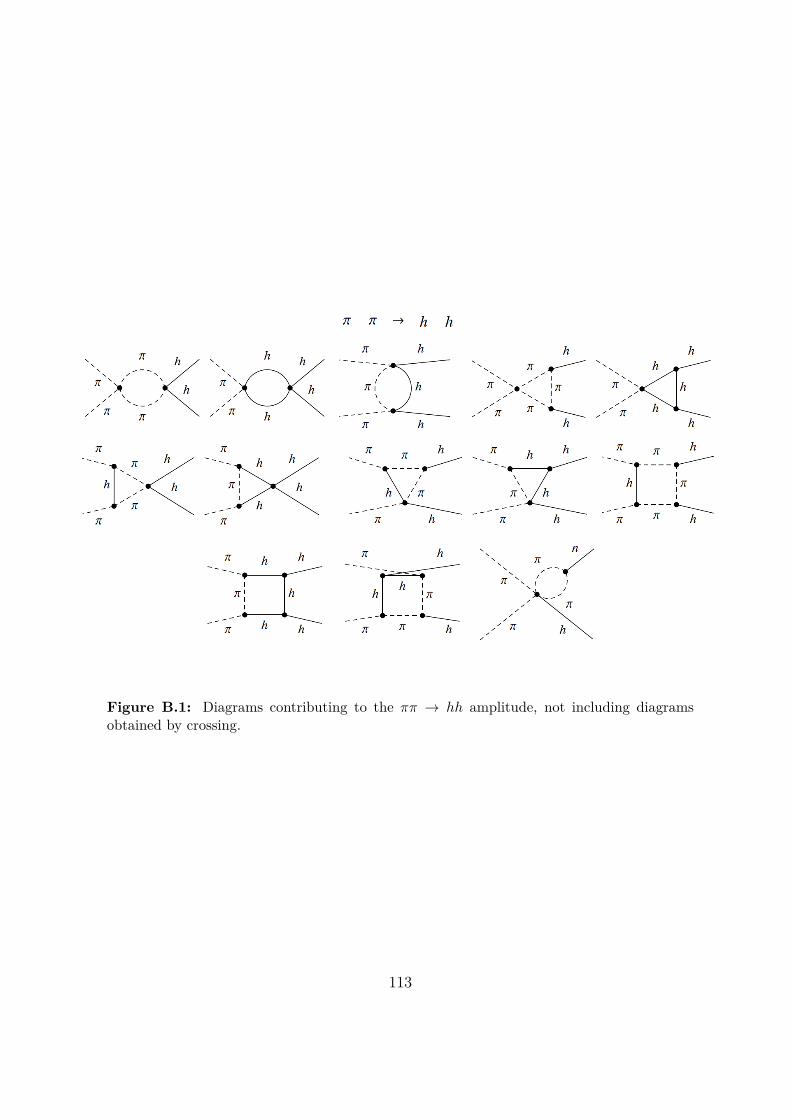
Figure B.1: Diagrams contributing to the fifi æ hh amplitude, not including diagramsobtained by crossing.

113

Figure B.2: Diagrams contributing to the fifi æ fifi amplitude, not including diagramsobtained by crossing.

counterterms correspond to

”bC = 12

1a2

C ≠ bC

2 5(4aC + 8aH) µ3

v≠ ⁄

≠ 218aCaH + 4a2

C + 12a2H ≠ bC ≠ 2bH

2 m2h

v2

6�Á,

”a7 = 18

5a2

C

1≠4a2

H ≠ 3bC + bH + 42

+ 2aCaHbC + bC

14a2

H ≠ bH ≠ 22

+ 4a4C

6�Á ,

”c8 = 13

Ëa2

C

1a2

H + bC

2≠ 2aCaHbC ≠ a3

CaH + a4C + b2

C

È�Á ,

”b9 = 14

Ë≠a2

C

1≠4a2

H + 5bC + bH

2≠ 4aCaHbC + 4a3

CaH + 4a4C + b2

C

È�Á ,

”a10 = 14

Ëa2

C

14a2

H + bC ≠ bH

2≠ 4aCaHbC ≠ 4a4

C + b2C

È�Á ,

”c20 = 112

5a2

C

12a2

H ≠ bC + 62

+ 2aCaHbC

≠ bC

13a2

H + bC + 62

≠ 2a3CaH + 2a4

C

6�Á .

(B.5)

For fifi æ fifi amplitudes, the relevant diagrams are displayed in Fig. B.2, and the requiredcounterterms are given by

”c6 = 148

Ëa2

C (6bC ≠ 8) ≠ 2a4C ≠ 3b2

C ≠ 2È

�Á,

”c11 = ≠ 112

1a2

C ≠ 122

�Á.(B.6)

114

Figure B.3: Diagrams contributing to the hh æ hh amplitude, not including diagramsobtained by crossing.

Finally, the relevant diagrams for hh æ hh amplitudes are shown in Fig. B.3, and the renormal-ization conditions read

”bH =512

3µ3

v

1≠40aHbH + 84a3

H

2≠ 13⁄a2

H + 3⁄bH

4

+187a2

HbH ≠ 120a4H ≠ 7b2

H

2 m2h

v2

6�Á,

”b⇤H = 14

Ë≠3

14a4

H + b2C

2+ 30a2

CbC + 10a2HbH ≠ 36a4

C ≠ b2H

È�Á,

”a�H = ≠34

1≠7a2

CbC + a2HbH + 6a4

C ≠ 2a4H + b2

C

2�Á,

”cDH =5

≠ 34

1a2

C ≠ bC

22 ≠ a4

H

4

6�Á,

”⁄ =; 3

2v2

Ë8µ2

3

16a2

H ≠ bH

2≠ 16⁄µ3vaH + ⁄2v2

È

≠ 121≠12µ3aHbH + 32µ3a

3H ≠ 6⁄va2

H + ⁄vbH

2 m2h

v3

+ 61≠48a2

HbH + 80a4H + 3b2

H

2 m4h

v4

<�Á.

(B.7)

115

Appendix C

The Renormalization Group Equations

This Appendix provides the expressions for the RGE of all couplings discussed above, at the orderconsidered.

16fi2 d

d ln µaC = aC

C15a2

H ≠ 3bC ≠ bH

2 m2h

v2 ≠ aHµ3

v

D

+ a2C

A

4aHm2

h

v2 ≠ µ3

v

B

+ 3a3C

m2h

v2 + bCµ3

v≠ 4aHbC

m2h

v2 , (C.1)

16fi2 d

d ln µbC = bC

C

215a2

C + 8aCaH + 17a2H ≠ 3bH

2 m2h

v2 + ⁄ ≠ 2(2aC + 5aH)µ3

v

D

≠ 2b2C

m2h

v2 + a2C

3≠⁄ + 4aC

µ3

v+ 8aH

µ3

v

4

≠ 4a2C

12a2

C + 4aCaH + 6a2H ≠ bH

2 m2h

v2 , (C.2)

16fi2 d

d ln µaH = aH

C

⁄ ≠1a2

C ≠ bC + 17bH

2 m2h

v2

D

≠ 12a2H

µ3

v+ 45a3

H

m2h

v2 + 2bHµ3

v, (C.3)

16fi2 d

d ln µbH = bH

C

21≠a2

C + 97a2H + bC

2 m2h

v2 ≠ 44aHµ3

v+ 3⁄

D

≠ 18b2H

m2h

v2

+ a2H

3≠13⁄ + 84aH

µ3

v

4≠ 240a4

H

m2h

v2 , (C.4)

16fi2 d

d ln µm2

h = m2h

3⁄ ≠ 10aH

µ3

v

4+

122a2

H ≠ 4bH

2 m4h

v2 + µ23 , (C.5)

16fi2 d

d ln µµ3 = µ3

C187a2

H ≠ 15bH

2 m2h

v2 + 3⁄

D

≠ 15aHµ2

3v

≠ 12⁄aHm2

h

v≠

196a3

H ≠ 36aHbH

2 m4h

v3 , (C.6)

16fi2 d

d ln µ⁄ = ⁄

C

4141a2

H ≠ 7bH

2 m2h

v2 ≠ 52aHµ3

v

D

+ 3⁄2 + 2416a2

H ≠ bH

2 µ23

v2

116

≠ 96aH

18a2

H ≠ 3bH

2 µ3m2h

v3 + 12180a4

H ≠ 48a2HbH + 3b2

H

2 m4h

v4 , (C.7)

16fi2 d

d ln µv2 = ≠2

1a2

C ≠ bC

2m2

h , (C.8)

16fi2 d

d ln µc6 = ≠ 1

24Ë2 + 2a4

C + 3b2C ≠ a2

C (≠8 + 6bC)È

, (C.9)

16fi2 d

d ln µc7 = ≠c7

C1a2

C ≠ 5a2H ≠ bC + bH

2 m2h

v2 + aHµ3

v

D

+ 12

1≠2aC ≠ a3

C + a2CaH ≠ aHbC

2, (C.10)

16fi2 d

d ln µa7 = ≠a7

C

21a2

C ≠ 5a2H ≠ bC + bH

2 m2h

v2 + 2aHµ3

v

D

+ 14

Ë4a4

C + 2aCaHbC + bC

1≠2 + 4a2

H ≠ bH

2+ a2

C

14 ≠ 4a2

H ≠ 3bC + bH

2È,

(C.11)

16fi2 d

d ln µc8 = ≠c8

C

21a2

C ≠ 5a2H ≠ bC + bH

2 m2h

v2 + 2aHµ3

v

D

+ 23

Ëa4

C ≠ a3CaH ≠ 2aCaHbC + b2

C + a2C

1a2

H + bC

2È, (C.12)

16fi2 d

d ln µc9 = a2

C

2 , (C.13)

16fi2 d

d ln µa9 = ≠a9

C1a2

C ≠ 5a2H ≠ bC + bH

2 m2h

v2 + aHµ3

v

D

≠ 12aC

1a2

C + aCaH ≠ bC

2, (C.14)

16fi2 d

d ln µb9 = ≠b9

C

21a2

C ≠ 5a2H ≠ bC + bH

2 m2h

v2 + 2aHµ3

v

D

+ 12

Ë4a4

C + 4a3CaH ≠ 4aCaHbC + b2

C + a2C

14a2

H ≠ 5bC ≠ bH

2È, (C.15)

16fi2 d

d ln µc10 = ≠c10

C1a2

C ≠ 5a2H ≠ bC + bH

2 m2h

v2 + aHµ3

v

D

+ aC

1a2

C ≠ aCaH + bC

2, (C.16)

16fi2 d

d ln µa10 = ≠a10

C

21a2

C ≠ 5a2H ≠ bC + bH

2 m2h

v2 + 2aHµ3

v

D

+ 12

1≠4a4

C ≠ 4aCaHbC + b2C + a2

C

14a2

H + bC ≠ bH

22, (C.17)

16fi2 d

d ln µc11 = ≠1

61a2

C ≠ 122

, (C.18)

16fi2 d

d ln µc20 = ≠c20

C

21a2

C ≠ 5a2H ≠ bC + bH

2 m2h

v2 + 2aHµ3

v

D

(C.19)

+ 16

Ë2a4

C ≠ 2a3CaH + a2

C

16 + 2a2

H ≠ bC

2+ 2aCaHbC ≠ bC

16 + 3a2

H + bC

2È,

117

16fi2 d

d ln µc⇤H = ≠c⇤H

C

21a2

C ≠ 5a2H ≠ bC + bH

2 m2h

v2 + 2aHµ3

v

D

+ 12

1≠3a2

C ≠ a2H

2, (C.20)

16fi2 d

d ln µa⇤H = ≠a⇤H

C

31a2

C ≠ 5a2H ≠ bC + bH

2 m2h

v2 + 3aHµ3

v

D

+ 3a3C + a3

H ≠ 3aCbC

2 ≠ aHbH

2 , (C.21)

16fi2 d

d ln µb⇤H = ≠b⇤H

C

41a2

C ≠ 5a2H ≠ bC + bH

2 m2h

v2 + 4aHµ3

v

D

≠ 18a4C ≠ 6a4

H + 15a2CbC ≠ 3b2

C

2 + 5a2HbH ≠ b2

H

2 , (C.22)

16fi2 d

d ln µc�H = ≠c�H

C

31a2

C ≠ 5a2H ≠ bC + bH

2 m2h

v2 + 3aHµ3

v

D

+ 3a3C ≠ a3

H ≠ 3aCbC , (C.23)

16fi2 d

d ln µa�H = ≠a�H

C

41a2

C ≠ 5a2H ≠ bC + bH

2 m2h

v2 + 4aHµ3

v

D

≠ 32

16a4

C ≠ 2a4H ≠ 7a2

CbC + b2C + a2

HbH

2, (C.24)

16fi2 d

d ln µcDH = ≠cDH

C

41a2

C ≠ 5a2H ≠ bC + bH

2 m2h

v2 + 4aHµ3

v

D

≠ 12

5a4

H + 31a2

C ≠ bC

226

. (C.25)

118

Bibliography

[1] ATLAS collaboration, G. Aad et al., Observation of a new particle in the search for theStandard Model Higgs boson with the ATLAS detector at the LHC, Phys. Lett. B716 (2012)1–29, [1207.7214].

[2] CMS collaboration, S. Chatrchyan et al., Observation of a new boson at a mass of 125GeV with the CMS experiment at the LHC, Phys. Lett. B716 (2012) 30–61, [1207.7235].

[3] D. B. Kaplan, H. Georgi and S. Dimopoulos, Composite Higgs Scalars, Phys. Lett. B136(1984) 187–190.

[4] D. B. Kaplan and H. Georgi, SU(2) x U(1) Breaking by Vacuum Misalignment, Phys. Lett.B136 (1984) 183–186.

[5] H. Georgi and D. B. Kaplan, Composite Higgs and Custodial SU(2), Phys. Lett. B145(1984) 216–220.

[6] H. Georgi, D. B. Kaplan and P. Galison, Calculation of the Composite Higgs Mass, Phys.Lett. B143 (1984) 152–154.

[7] T. Banks, Constraints on SU(2) x U(1) breaking by vacuum misalignment, Nucl. Phys.B243 (1984) 125–130.

[8] M. J. Dugan, H. Georgi and D. B. Kaplan, Anatomy of a Composite Higgs Model, Nucl.Phys. B254 (1985) 299–326.

[9] K. Agashe, R. Contino and A. Pomarol, The Minimal composite Higgs model, Nucl. Phys.B719 (2005) 165–187, [hep-ph/0412089].

[10] R. Contino, L. Da Rold and A. Pomarol, Light custodians in natural composite Higgsmodels, Phys. Rev. D75 (2007) 055014, [hep-ph/0612048].

[11] B. Gripaios, A. Pomarol, F. Riva and J. Serra, Beyond the Minimal Composite HiggsModel, JHEP 04 (2009) 070, [0902.1483].

[12] H. Gertov, A. Meroni, E. Molinaro and F. Sannino, Theory and phenomenology of theelementary Goldstone Higgs boson, Phys. Rev. D92 (2015) 095003, [1507.06666].

[13] M. Frigerio, A. Pomarol, F. Riva and A. Urbano, Composite Scalar Dark Matter, JHEP 07(2012) 015, [1204.2808].

119

[14] D. Marzocca and A. Urbano, Composite Dark Matter and LHC Interplay, JHEP 07 (2014)107, [1404.7419].

[15] G. Panico, M. Redi, A. Tesi and A. Wulzer, On the Tuning and the Mass of the CompositeHiggs, JHEP 03 (2013) 051, [1210.7114].

[16] M. Carena, L. Da Rold and E. Pontón, Minimal Composite Higgs Models at the LHC,JHEP 06 (2014) 159, [1402.2987].

[17] R. Contino, D. Marzocca, D. Pappadopulo and R. Rattazzi, On the e�ect of resonances incomposite Higgs phenomenology, JHEP 10 (2011) 081, [1109.1570].

[18] D. Marzocca, M. Serone and J. Shu, General Composite Higgs Models, JHEP 08 (2012)013, [1205.0770].

[19] M. Redi and A. Tesi, Implications of a Light Higgs in Composite Models, JHEP 10 (2012)166, [1205.0232].

[20] A. Carmona and F. Goertz, A naturally light Higgs without light Top Partners, JHEP 05(2015) 002, [1410.8555].

[21] G. von Gersdor�, E. Pontón and R. Rosenfeld, The Dynamical Composite Higgs, JHEP 06(2015) 119, [1502.07340].

[22] R. Barbieri, B. Bellazzini, V. S. Rychkov and A. Varagnolo, The Higgs boson from anextended symmetry, Phys. Rev. D76 (2007) 115008, [0706.0432].

[23] T. Alanne, H. Gertov, A. Meroni and F. Sannino, Vacuum alignment with and withoutelementary scalars, Phys. Rev. D94 (2016) 075015, [1608.07442].

[24] G. Buchalla, O. Cata, A. Celis and C. Krause, Standard Model Extended by a HeavySinglet: Linear vs. Nonlinear EFT, 1608.03564.

[25] S. Fichet, G. von Gersdor�, E. Pontón and R. Rosenfeld, The Global Higgs as a Signal forCompositeness at the LHC, JHEP 01 (2017) 012, [1608.01995].

[26] S. Fichet, G. von Gersdor�, E. Pontón and R. Rosenfeld, The Excitation of the GlobalSymmetry-Breaking Vacuum in Composite Higgs Models, JHEP 09 (2016) 158,[1607.03125].

[27] K. Kannike, G. M. Pelaggi, A. Salvio and A. Strumia, The Higgs of the Higgs and thediphoton channel, JHEP 07 (2016) 101, [1605.08681].

[28] M. Gell-Mann and M. Levy, The axial vector current in beta decay, Nuovo Cim. 16 (1960)705.

[29] D. B. Kaplan, Flavor at SSC energies: A New mechanism for dynamically generatedfermion masses, Nucl. Phys. B365 (1991) 259–278.

120

[30] M. B. Gavela, K. Kanshin, P. A. N. Machado and S. Saa, On the renormalization of theelectroweak chiral Lagrangian with a Higgs, JHEP 03 (2015) 043, [1409.1571].

[31] F. Feruglio, B. Gavela, K. Kanshin, P. A. N. Machado, S. Rigolin and S. Saa, The minimallinear sigma model for the Goldstone Higgs, JHEP 06 (2016) 038, [1603.05668].

[32] M. B. Gavela, K. Kanshin, P. A. N. Machado and S. Saa, The linear–non-linear frontier forthe Goldstone Higgs, Eur. Phys. J. C76 (2016) 690, [1610.08083].

[33] S. L. Glashow, Partial Symmetries of Weak Interactions, Nucl. Phys. 22 (1961) 579–588.

[34] S. Weinberg, A Model of Leptons, Phys. Rev. Lett. 19 (1967) 1264–1266.

[35] A. Salam, Weak and Electromagnetic Interactions, Conf. Proc. C680519 (1968) 367–377.

[36] P. W. Higgs, Broken symmetries, massless particles and gauge fields, Phys. Lett. 12 (1964)132–133.

[37] P. W. Higgs, Broken Symmetries and the Masses of Gauge Bosons, Phys. Rev. Lett. 13(1964) 508–509.

[38] F. Englert and R. Brout, Broken Symmetry and the Mass of Gauge Vector Mesons, Phys.Rev. Lett. 13 (1964) 321–323.

[39] G. S. Guralnik, C. R. Hagen and T. W. B. Kibble, Global Conservation Laws and MasslessParticles, Phys. Rev. Lett. 13 (1964) 585–587.

[40] J. C. Romao and J. P. Silva, A resource for signs and Feynman diagrams of the StandardModel, Int. J. Mod. Phys. A27 (2012) 1230025, [1209.6213].

[41] ATLAS, CMS collaboration, G. Aad et al., Combined Measurement of the Higgs BosonMass in pp Collisions at

Ôs = 7 and 8 TeV with the ATLAS and CMS Experiments, Phys.

Rev. Lett. 114 (2015) 191803, [1503.07589].

[42] P. Sikivie, L. Susskind, M. B. Voloshin and V. I. Zakharov, Isospin Breaking in TechnicolorModels, Nucl. Phys. B173 (1980) 189–207.

[43] G. ’t Hooft, Renormalizable Lagrangians for Massive Yang-Mills Fields, Nucl. Phys. B35(1971) 167–188.

[44] M. Schmaltz, Physics beyond the standard model (theory): Introducing the little Higgs,Nucl. Phys. Proc. Suppl. 117 (2003) 40–49, [hep-ph/0210415].

[45] L. Susskind, Dynamics of Spontaneous Symmetry Breaking in the Weinberg-Salam Theory,Phys. Rev. D20 (1979) 2619–2625.

[46] G. ’t Hooft and M. J. G. Veltman, Regularization and Renormalization of Gauge Fields,Nucl. Phys. B44 (1972) 189–213.

[47] A. Salvio and A. Strumia, Agravity, JHEP 06 (2014) 080, [1403.4226].

121

[48] G. ’t Hooft, Naturalness, chiral symmetry, and spontaneous chiral symmetry breaking,NATO Sci. Ser. B 59 (1980) 135–157.

[49] Y. Nambu, Quasiparticles and Gauge Invariance in the Theory of Superconductivity, Phys.Rev. 117 (1960) 648–663.

[50] J. Goldstone, Field Theories with Superconductor Solutions, Nuovo Cim. 19 (1961)154–164.

[51] J. Goldstone, A. Salam and S. Weinberg, Broken Symmetries, Phys. Rev. 127 (1962)965–970.

[52] H. Yukawa, On the Interaction of Elementary Particles I, Proc. Phys. Math. Soc. Jap. 17(1935) 48–57.

[53] J. F. Donoghue, E. Golowich and B. R. Holstein, Dynamics of the standard model, Camb.Monogr. Part. Phys. Nucl. Phys. Cosmol. 2 (1992) 1–540.

[54] Particle Data Group collaboration, C. Patrignani et al., Review of Particle Physics,Chin. Phys. C40 (2016) 100001.

[55] S. Weinberg, Nonlinear realizations of chiral symmetry, Phys. Rev. 166 (1968) 1568–1577.

[56] J. Gasser and H. Leutwyler, Chiral Perturbation Theory to One Loop, Annals Phys. 158(1984) 142.

[57] S. Weinberg, Phenomenological Lagrangians, Physica A96 (1979) 327–340.

[58] A. Manohar and H. Georgi, Chiral Quarks and the Nonrelativistic Quark Model, Nucl.Phys. B234 (1984) 189–212.

[59] H. Georgi, Weak Interactions and Modern Particle Theory. 1984.

[60] T. Das, G. S. Guralnik, V. S. Mathur, F. E. Low and J. E. Young, Electromagnetic massdi�erence of pions, Phys. Rev. Lett. 18 (1967) 759–761.

[61] S. Weinberg, Implications of Dynamical Symmetry Breaking, Phys. Rev. D13 (1976)974–996.

[62] S. Weinberg, Implications of Dynamical Symmetry Breaking: An Addendum, Phys. Rev.D19 (1979) 1277–1280.

[63] E. Eichten and K. D. Lane, Dynamical Breaking of Weak Interaction Symmetries, Phys.Lett. B90 (1980) 125–130.

[64] S. Dimopoulos and L. Susskind, Mass Without Scalars, Nucl. Phys. B155 (1979) 237–252.

[65] M. E. Peskin and T. Takeuchi, Estimation of oblique electroweak corrections, Phys. Rev.D46 (1992) 381–409.

122

[66] B. Holdom and J. Terning, Large corrections to electroweak parameters in technicolortheories, Phys. Lett. B247 (1990) 88–92.

[67] M. Golden and L. Randall, Radiative Corrections to Electroweak Parameters in TechnicolorTheories, Nucl. Phys. B361 (1991) 3–23.

[68] R. Contino, The Higgs as a Composite Nambu-Goldstone Boson, in Physics of the largeand the small, TASI 09, proceedings of the Theoretical Advanced Study Institute inElementary Particle Physics, Boulder, Colorado, USA, 1-26 June 2009, pp. 235–306, 2011.1005.4269. DOI.

[69] G. Panico and A. Wulzer, The Composite Nambu-Goldstone Higgs, Lect. Notes Phys. 913(2016) pp.1–316, [1506.01961].

[70] R. Alonso, I. Brivio, B. Gavela, L. Merlo and S. Rigolin, Sigma Decomposition, JHEP 12(2014) 034, [1409.1589].

[71] S. R. Coleman and E. J. Weinberg, Radiative Corrections as the Origin of SpontaneousSymmetry Breaking, Phys. Rev. D7 (1973) 1888–1910.

[72] S. R. Coleman, J. Wess and B. Zumino, Structure of phenomenological Lagrangians. 1.,Phys. Rev. 177 (1969) 2239–2247.

[73] C. G. Callan, Jr., S. R. Coleman, J. Wess and B. Zumino, Structure of phenomenologicalLagrangians. 2., Phys. Rev. 177 (1969) 2247–2250.

[74] N. Arkani-Hamed, A. G. Cohen and H. Georgi, Electroweak symmetry breaking fromdimensional deconstruction, Phys. Lett. B513 (2001) 232–240, [hep-ph/0105239].

[75] N. Arkani-Hamed, A. G. Cohen, T. Gregoire and J. G. Wacker, Phenomenology ofelectroweak symmetry breaking from theory space, JHEP 08 (2002) 020, [hep-ph/0202089].

[76] M. Schmaltz and D. Tucker-Smith, Little Higgs review, Ann. Rev. Nucl. Part. Sci. 55(2005) 229–270, [hep-ph/0502182].

[77] G. Ferretti and D. Karateev, Fermionic UV completions of Composite Higgs models, JHEP03 (2014) 077, [1312.5330].

[78] G. Ferretti, UV Completions of Partial Compositeness: The Case for a SU(4) GaugeGroup, JHEP 06 (2014) 142, [1404.7137].

[79] G. Cacciapaglia and F. Sannino, Fundamental Composite (Goldstone) Higgs Dynamics,JHEP 04 (2014) 111, [1402.0233].

[80] T. Appelquist and J. Carazzone, Infrared Singularities and Massive Fields, Phys. Rev. D11(1975) 2856.

[81] B. Henning, X. Lu and H. Murayama, How to use the Standard Model e�ective field theory,JHEP 01 (2016) 023, [1412.1837].

123

[82] LHC Higgs Cross Section Working Group collaboration, D. de Florian et al.,Handbook of LHC Higgs Cross Sections: 4. Deciphering the Nature of the Higgs Sector,1610.07922.

[83] S. Weinberg, Baryon and Lepton Nonconserving Processes, Phys. Rev. Lett. 43 (1979)1566–1570.

[84] G. Passarino, Field reparametrization in e�ective field theories, Eur. Phys. J. Plus 132(2017) 16, [1610.09618].

[85] W. Buchmuller and D. Wyler, E�ective Lagrangian Analysis of New Interactions andFlavor Conservation, Nucl. Phys. B268 (1986) 621–653.

[86] K. Hagiwara, S. Ishihara, R. Szalapski and D. Zeppenfeld, Low-energy e�ects of newinteractions in the electroweak boson sector, Phys. Rev. D48 (1993) 2182–2203.

[87] G. F. Giudice, C. Grojean, A. Pomarol and R. Rattazzi, The Strongly-Interacting LightHiggs, JHEP 06 (2007) 045, [hep-ph/0703164].

[88] B. Grzadkowski, M. Iskrzynski, M. Misiak and J. Rosiek, Dimension-Six Terms in theStandard Model Lagrangian, JHEP 10 (2010) 085, [1008.4884].

[89] T. Appelquist and C. W. Bernard, Strongly Interacting Higgs Bosons, Phys. Rev. D22(1980) 200.

[90] A. C. Longhitano, Heavy Higgs Bosons in the Weinberg-Salam Model, Phys. Rev. D22(1980) 1166.

[91] A. C. Longhitano, Low-Energy Impact of a Heavy Higgs Boson Sector, Nucl. Phys. B188(1981) 118–154.

[92] F. Feruglio, The Chiral approach to the electroweak interactions, Int. J. Mod. Phys. A8(1993) 4937–4972, [hep-ph/9301281].

[93] R. Alonso, M. B. Gavela, L. Merlo, S. Rigolin and J. Yepes, The E�ective ChiralLagrangian for a Light Dynamical "Higgs Particle", Phys. Lett. B722 (2013) 330–335,[1212.3305].

[94] B. Grinstein and M. Trott, A Higgs-Higgs bound state due to new physics at a TeV, Phys.Rev. D76 (2007) 073002, [0704.1505].

[95] R. Contino, C. Grojean, M. Moretti, F. Piccinini and R. Rattazzi, Strong Double HiggsProduction at the LHC, JHEP 05 (2010) 089, [1002.1011].

[96] A. Azatov, R. Contino and J. Galloway, Model-Independent Bounds on a Light Higgs,JHEP 04 (2012) 127, [1202.3415].

[97] G. Buchalla, O. Catà and C. Krause, Complete Electroweak Chiral Lagrangian with a LightHiggs at NLO, Nucl. Phys. B880 (2014) 552–573, [1307.5017].

124

[98] M. B. Gavela, J. Gonzalez-Fraile, M. C. Gonzalez-Garcia, L. Merlo, S. Rigolin andJ. Yepes, CP violation with a dynamical Higgs, JHEP 10 (2014) 044, [1406.6367].

[99] L. Merlo, S. Saa and M. S. Barbero, Baryon Non-Invariant Couplings in Higgs E�ectiveField Theory, 1612.04832.

[100] A. G. Cohen, D. B. Kaplan and A. E. Nelson, Counting 4 pis in strongly coupledsupersymmetry, Phys. Lett. B412 (1997) 301–308, [hep-ph/9706275].

[101] M. A. Luty, Naive dimensional analysis and supersymmetry, Phys. Rev. D57 (1998)1531–1538, [hep-ph/9706235].

[102] B. M. Gavela, E. E. Jenkins, A. V. Manohar and L. Merlo, Analysis of General PowerCounting Rules in E�ective Field Theory, Eur. Phys. J. C76 (2016) 485, [1601.07551].

[103] I. Brivio, T. Corbett, O. J. P. Éboli, M. B. Gavela, J. Gonzalez-Fraile, M. C.Gonzalez-Garcia et al., Disentangling a dynamical Higgs, JHEP 03 (2014) 024,[1311.1823].

[104] R. Alonso, M. B. Gavela, L. Merlo, S. Rigolin and J. Yepes, Minimal Flavour Violationwith Strong Higgs Dynamics, JHEP 06 (2012) 076, [1201.1511].

[105] G. Buchalla, O. Cata and C. Krause, A Systematic Approach to the SILH Lagrangian,Nucl. Phys. B894 (2015) 602–620, [1412.6356].

[106] I. M. Hierro, L. Merlo and S. Rigolin, Sigma Decomposition: The CP-Odd Lagrangian,JHEP 04 (2016) 016, [1510.07899].

[107] I. Brivio, J. Gonzalez-Fraile, M. C. Gonzalez-Garcia and L. Merlo, The complete HEFTLagrangian after the LHC Run I, Eur. Phys. J. C76 (2016) 416, [1604.06801].

[108] O. J. P. Éboli and M. C. Gonzalez–Garcia, Classifying the bosonic quartic couplings, Phys.Rev. D93 (2016) 093013, [1604.03555].

[109] L. J. Dixon and Y. Li, Bounding the Higgs Boson Width Through Interferometry, Phys.Rev. Lett. 111 (2013) 111802, [1305.3854].

[110] Particle Data Group collaboration, K. A. Olive et al., Review of Particle Physics,Chin. Phys. C38 (2014) 090001.

[111] J. F. Gunion, H. E. Haber, G. L. Kane and S. Dawson, The Higgs Hunter’s Guide, Front.Phys. 80 (2000) 1–404.

[112] K. Agashe, R. Contino, L. Da Rold and A. Pomarol, A Custodial symmetry for Zbb, Phys.Lett. B641 (2006) 62–66, [hep-ph/0605341].

[113] ATLAS, CMS collaboration, Measurements of the Higgs boson production and decay ratesand constraints on its couplings from a combined ATLAS and CMS analysis of the LHC ppcollision data at

Ôs = 7 and 8 TeV, .

125

[114] C. Anastasiou, E. Furlan and J. Santiago, Realistic Composite Higgs Models, Phys. Rev.D79 (2009) 075003, [0901.2117].

[115] D. Ghosh, M. Salvarezza and F. Senia, Extending the Analysis of Electroweak PrecisionConstraints in Composite Higgs Models, Nucl. Phys. B914 (2017) 346–387, [1511.08235].

[116] G. Altarelli and R. Barbieri, Vacuum polarization e�ects of new physics on electroweakprocesses, Phys. Lett. B253 (1991) 161–167.

[117] M. Ciuchini, E. Franco, S. Mishima, M. Pierini, L. Reina and L. Silvestrini, Update of theelectroweak precision fit, interplay with Higgs-boson signal strengths and model-independentconstraints on new physics, Nucl. Part. Phys. Proc. 273-275 (2016) 2219–2225,[1410.6940].

[118] V. A. Novikov, L. B. Okun and M. I. Vysotsky, On the Electroweak one loop corrections,Nucl. Phys. B397 (1993) 35–83.

[119] A. Orgogozo and S. Rychkov, The S parameter for a Light Composite Higgs: a DispersionRelation Approach, JHEP 06 (2013) 014, [1211.5543].

[120] H. E. Haber and D. O’Neil, Basis-independent methods for the two-Higgs-doublet model III:The CP-conserving limit, custodial symmetry, and the oblique parameters S, T, U, Phys.Rev. D83 (2011) 055017, [1011.6188].

[121] L. Lavoura and J. P. Silva, The Oblique corrections from vector - like singlet and doubletquarks, Phys. Rev. D47 (1993) 2046–2057.

[122] ATLAS collaboration, G. Aad et al., Search for production of vector-like quark pairs andof four top quarks in the lepton-plus-jets final state in pp collisions at

Ôs = 8 TeV with the

ATLAS detector, JHEP 08 (2015) 105, [1505.04306].

[123] CMS collaboration, C. Collaboration, Search for top quark partners with charge 5/3 atÔs = 13 TeV, .

[124] S. Dawson and E. Furlan, A Higgs Conundrum with Vector Fermions, Phys. Rev. D86(2012) 015021, [1205.4733].

[125] LHC Higgs Cross Section Working Group collaboration, J. R. Andersen et al.,Handbook of LHC Higgs Cross Sections: 3. Higgs Properties, 1307.1347.

[126] ATLAS collaboration, G. Aad et al., Search for Scalar Diphoton Resonances in the MassRange 65 ≠ 600 GeV with the ATLAS Detector in pp Collision Data at

Ôs = 8 TeV , Phys.

Rev. Lett. 113 (2014) 171801, [1407.6583].

[127] CMS collaboration, V. Khachatryan et al., Search for diphoton resonances in the massrange from 150 to 850 GeV in pp collisions at

Ôs = 8 TeV, Phys. Lett. B750 (2015)

494–519, [1506.02301].

126

[128] ATLAS collaboration, G. Aad et al., Search for a high-mass Higgs boson decaying to a Wboson pair in pp collisions at

Ôs = 8 TeV with the ATLAS detector, JHEP 01 (2016) 032,

[1509.00389].

[129] ATLAS collaboration, G. Aad et al., Search for an additional, heavy Higgs boson in theH æ ZZ decay channel at

Ôs = 8 TeV in pp collision data with the ATLAS detector,

Eur. Phys. J. C76 (2016) 45, [1507.05930].

[130] CMS collaboration, Properties of the Higgs-like boson in the decay H to ZZ to 4l in ppcollisions at sqrt s =7 and 8 TeV, .

[131] CMS collaboration, Update on the search for the standard model Higgs boson in ppcollisions at the LHC decaying to W + W in the fully leptonic final state, .

[132] CMS collaboration, V. Khachatryan et al., Search for resonant pair production of Higgsbosons decaying to two bottom quark–antiquark pairs in proton–proton collisions at 8 TeV,Phys. Lett. B749 (2015) 560–582, [1503.04114].

[133] ATLAS collaboration, G. Aad et al., Searches for Higgs boson pair production in thehh æ bb··, ““WW ú, ““bb, bbbb channels with the ATLAS detector, Phys. Rev. D92 (2015)092004, [1509.04670].

[134] ATLAS, CMS collaboration, A. Holzner, Beyond standard model Higgs physics: prospectsfor the High Luminosity LHC, 1411.0322.

[135] V. Martín Lozano, J. M. Moreno and C. B. Park, Resonant Higgs boson pair production inthe hh æ bb WW æ bb¸+‹¸≠‹ decay channel, JHEP 08 (2015) 004, [1501.03799].

[136] ATLAS collaboration, Search for resonances decaying to photon pairs in 3.2 fb≠1 of ppcollisions at

Ôs = 13 TeV with the ATLAS detector, .

[137] CMS collaboration, C. Collaboration, Search for new physics in high mass diphoton eventsin proton-proton collisions at 13TeV, .

[138] ATLAS collaboration, G. Aad et al., Evidence for Electroweak Production of W ±W ±jj inpp Collisions at

Ôs = 8 TeV with the ATLAS Detector, Phys. Rev. Lett. 113 (2014)

141803, [1405.6241].

[139] ATLAS collaboration, G. Aad et al., Measurements of W ±Z production cross sections inpp collisions at

Ôs = 8 TeV with the ATLAS detector and limits on anomalous gauge boson

self-couplings, Phys. Rev. D93 (2016) 092004, [1603.02151].

[140] R. S. Chivukula and H. Georgi, Composite Technicolor Standard Model, Phys. Lett. B188(1987) 99–104.

[141] G. D’Ambrosio, G. F. Giudice, G. Isidori and A. Strumia, Minimal flavor violation: AnE�ective field theory approach, Nucl. Phys. B645 (2002) 155–187, [hep-ph/0207036].

[142] B. Grinstein, M. Redi and G. Villadoro, Low Scale Flavor Gauge Symmetries, JHEP 11(2010) 067, [1009.2049].

127

[143] R. L. Delgado, A. Dobado and F. J. Llanes-Estrada, One-loop WLWL and ZLZL scatteringfrom the electroweak Chiral Lagrangian with a light Higgs-like scalar, JHEP 02 (2014) 121,[1311.5993].

[144] D. Espriu, F. Mescia and B. Yencho, Radiative corrections to WL WL scattering incomposite Higgs models, Phys. Rev. D88 (2013) 055002, [1307.2400].

[145] R. L. Delgado, A. Dobado, M. J. Herrero and J. J. Sanz-Cillero, One-loop ““ æ W+L W≠

L

and ““ æ ZL ZL from the Electroweak Chiral Lagrangian with a light Higgs-like scalar,JHEP 07 (2014) 149, [1404.2866].

[146] F.-K. Guo, P. Ruiz-Femenía and J. J. Sanz-Cillero, One loop renormalization of theelectroweak chiral Lagrangian with a light Higgs boson, Phys. Rev. D92 (2015) 074005,[1506.04204].

[147] E. E. Jenkins, A. V. Manohar and M. Trott, Naive Dimensional Analysis Counting ofGauge Theory Amplitudes and Anomalous Dimensions, Phys. Lett. B726 (2013) 697–702,[1309.0819].

[148] T. Appelquist and C. W. Bernard, The Nonlinear ‡ Model in the Loop Expansion, Phys.Rev. D23 (1981) 425.

[149] I. S. Gerstein, R. Jackiw, S. Weinberg and B. W. Lee, Chiral loops, Phys. Rev. D3 (1971)2486–2492.

[150] J. M. Charap, Closed-loop calculations using a chiral-invariant lagrangian, Phys. Rev. D2(1970) 1554–1561.

[151] D. I. Kazakov, V. N. Pervushin and S. V. Pushkin, Invariant Renormalization for the FieldTheories with Nonlinear Symmetry, Teor. Mat. Fiz. 31 (1977) 169–176.

[152] D. I. Kazakov, V. N. Pervushin and S. V. Pushkin, An Invariant Renormalization Methodfor Nonlinear Realizations of the Dynamical Symmetries, Theor. Math. Phys. 31 (1977)389.

[153] B. de Wit and M. T. Grisaru, On-shell Counterterms and Nonlinear Invariances, Phys.Rev. D20 (1979) 2082.

[154] J. Honerkamp, Chiral multiloops, Nucl. Phys. B36 (1972) 130–140.

[155] R. Alonso, E. E. Jenkins and A. V. Manohar, A Geometric Formulation of Higgs E�ectiveField Theory: Measuring the Curvature of Scalar Field Space, Phys. Lett. B754 (2016)335–342, [1511.00724].

[156] R. Alonso, E. E. Jenkins and A. V. Manohar, Geometry of the Scalar Sector, JHEP 08(2016) 101, [1605.03602].

[157] R. Mertig, M. Bohm and A. Denner, FEYN CALC: Computer algebraic calculation ofFeynman amplitudes, Comput. Phys. Commun. 64 (1991) 345–359.

128

[158] A. Alloul, N. D. Christensen, C. Degrande, C. Duhr and B. Fuks, FeynRules 2.0 - Acomplete toolbox for tree-level phenomenology, Comput. Phys. Commun. 185 (2014)2250–2300, [1310.1921].

[159] J. Kublbeck, M. Bohm and A. Denner, Feyn Arts: Computer Algebraic Generation ofFeynman Graphs and Amplitudes, Comput. Phys. Commun. 60 (1990) 165–180.

[160] T. Hahn, Generating Feynman diagrams and amplitudes with FeynArts 3, Comput. Phys.Commun. 140 (2001) 418–431, [hep-ph/0012260].

[161] T. Hahn and M. Perez-Victoria, Automatized one loop calculations in four-dimensions andD-dimensions, Comput. Phys. Commun. 118 (1999) 153–165, [hep-ph/9807565].

[162] M. Ostrogradsky, Mémoire sur les équations di�érentielles relatives an probléme desisopérimétres. 1850.

[163] C. Grosse-Knetter, E�ective Lagrangians with higher derivatives and equations of motion,Phys. Rev. D49 (1994) 6709–6719, [hep-ph/9306321].

[164] S. Scherer and H. W. Fearing, Field transformations and the classical equation of motion inchiral perturbation theory, Phys. Rev. D52 (1995) 6445–6450, [hep-ph/9408298].

[165] C. Arzt, Reduced e�ective Lagrangians, Phys. Lett. B342 (1995) 189–195,[hep-ph/9304230].

129

The Goldstone Boson Higgs and the eective...

Documents

Transcript of The Goldstone Boson Higgs and the eective...