Universität Basel Peter Merian-Weg 6 4052 Basel, Switzerland wwz.unibas.ch

Corresponding Author: Conny Wunsch conny.wunsch@unibas.ch Tel: +41 61 207 33 74

February 2021

The Gender Pay Gap Revisited with Big Data: Do Methodological Choices Matter?

WWZ Working Paper 2021/05 Anthony Strittmatter, Conny Wunsch

A publication of the Center of Business and Economics (WWZ), University of Basel. WWZ 2021 and the authors. Reproduction for other purposes than the personal use needs the permission of the authors.

The Gender Pay Gap Revisited with Big Data:

Do Methodological Choices Matter?∗

Anthony Strittmatter† Conny Wunsch‡

February 18, 2021

Abstract

The vast majority of existing studies that estimate the average unexplained gender pay gap

use unnecessarily restrictive linear versions of the Blinder-Oaxaca decomposition. Using a

notably rich and large data set of 1.7 million employees in Switzerland, we investigate how

the methodological improvements made possible by such big data affect estimates of the

unexplained gender pay gap. We study the sensitivity of the estimates with regard to i)

the availability of observationally comparable men and women, ii) model flexibility when

controlling for wage determinants, and iii) the choice of different parametric and semi-

parametric estimators, including variants that make use of machine learning methods. We

find that these three factors matter greatly. Blinder-Oaxaca estimates of the unexplained

gender pay gap decline by up to 39% when we enforce comparability between men and

women and use a more flexible specification of the wage equation. Semi-parametric match-

ing yields estimates that when compared with the Blinder-Oaxaca estimates, are up to 50%

smaller and also less sensitive to the way wage determinants are included.

Keywords: Gender Inequality, Gender Pay Gap, Common Support, Model Specification,

Matching Estimator, Machine Learning.

JEL classification: J31, C21

∗We acknowledge helpful comments by Philipp Bach, Marina Bonaccolto-Topfer, Christina Felfe, Martin

Huber, Pat Kline, Michael Knaus, Matthias Krapf, and Michael Lechner, seminar participants at the University

of Basel, University of Linz, and LISER, Luxemburg, as well as conference participants at EALE/SOLE 2020,

Verein fur Socialpolitik 2020, and the IAB 2020 workshop on “Machine Learning in Labor, Education, and Health

Economics”. Anthony Strittmatter gratefully acknowledges financial support from the Swiss National Science

Foundation (Spark Project 190422) and the French National Research Agency (LabEx Ecodec/ANR-11-LABX-

0047). The authors are solely responsible for the analysis and the interpretation thereof.†CREST-ENSAE, Institut Polytechnique Paris, France; CESifo, Munich, Germany; email: an-

thony.strittmatter@ensae.fr.‡Faculty of Business and Economics, University of Basel; University St. Gallen, Switzerland; email:

conny.wunsch@unibas.ch.

1 Introduction

Achieving gender equality, especially equality in pay, is among the top priorities for governments

in many countries. Measuring unexplained inequalities in pay between women and men, the so-

called unexplained gender pay gap, has been the subject of an extensive literature for more than

half a century (see Blau and Kahn, 2000, 2017; Goldin and Mitchell, 2017; Kunze, 2018; Olivetti

and Petrongolo, 2016, for comprehensive reviews). A large literature focuses on understanding

the sources of inequality in pay by studying the sensitivity of the gender pay gap with regard to

the inclusion of important wage determinants. A much smaller literature focuses on the impact

of methodological choices. We contribute to the latter literature by investigating the sensitivity

of the estimated gender pay gap with regard to three dimensions: enforcement of overlap in

wage determinants across gender, flexibility of model specification, and estimation method. Our

results suggest that these methodological choices can reduce the estimated unexplained gender

pay gap by as much as 50%, even when keeping relevant wage determinants fixed across estimates.

This suggests that methodological choices are at least as relevant for gender pay gap estimations

as considerations about wage determinants.

Weichselbaumer and Winter-Ebmer (2005) and Van der Velde et al. (2015) document that

the vast majority of existing studies use a linear version of the Blinder-Oaxaca decomposition

(BO, Blinder, 1973; Oaxaca, 1973) to estimate the mean unexplained gender pay gap (see Fortin

et al., 2011, for a comprehensive review of BO and other decomposition methods). Thus, BO

estimates serve as the key input for policy makers who aim to achieve equality in pay. However,

most applications of BO impose a number of restrictions that may not be realistic. Firstly, they

typically use relatively inflexible functional forms for the wage equation. For example, the returns

to education are often assumed to be the same across occupations, age and experience, which

contradicts both theory and empirical evidence (see, e.g., Lemieux, 2014). Secondly, standard

applications of BO do not account for common support violations, i.e., the lack of observationally

comparable men for every woman. BO extrapolates into regions without support based on the

assumed functional form. If the functional form is misspecified and there is lack of support, then

this extrapolation may lead to bias. Thirdly, BO restricts heterogeneity in gender pay gaps to

variable-specific differences in coefficients. Any heterogeneity that is not captured by this may

bias estimates of the mean gender pay gap. This is particularly relevant, because heterogeneity

in gender pay gaps is widely acknowledged in the literature (see, e.g., Bach et al., 2018; Baron

and Cobb-Clark, 2010; Bonjour and Gerfin, 2001; Chernozhukov et al., 2013, 2018a; Goldin,

2014).

Of course, these restrictions can easily be relaxed when working with large data sets. Re-

searchers can model the inclusion of control variables in more flexible ways. They can check

and enforce common support ex ante, even for parametric estimators like BO. Furthermore,

1

they can choose more flexible estimators that unlike BO do not restrict pay gap heterogene-

ity. Surprisingly though, these adjustments are rarely implemented in applied work. Therefore,

an important question we explore in this study is whether these adjustments really matter in

practice. To answer this question, we exploit a very large data set that covers about 37,000

establishments with individual data on more than 1.7 million employees in Switzerland, which

covers almost one third of all Swiss employees. The data allow us to take full advantage of the

methodological improvements that are possible with existing methods. In particular, they allow

us to go as far as exact matching on all elements of the rich set of observed wage determinants

with resulting cells that are still large enough for meaningful analysis after enforcing full support.

We start by analyzing common support and the gender pay gap obtained from exact matching

applying the technique of Nopo (2008). Thereafter, we estimate the mean unexplained gender

pay gap with different parametric and semi-parametric methods and for various samples that

differ in how strictly we impose common support. As estimators, we consider a linear regression

model (LRM) with a dummy for women, BO, inverse probability weighting (IPW), augmented

IPW (AIPW) as a doubly robust mixture between BO and IPW, propensity score matching

(PSM) and a combination of exact matching and PSM (EXPSM). For each estimator, we consider

three model specifications that differ in how flexibly we include the observed wage determinants:

(i) the baseline model contains dummy variables for all categories and quadratic terms for the

continuous variables (up to 117 control variables), (ii) the full model additionally contains higher-

order polynomials as well as a large number of interactions between wage determinants (up to 615

control variables), and (iii) the machine learning model employs LASSO estimation techniques

(Tibshirani, 1996) to select the relevant wage determinants in a data-driven way (see Hastie et

al., 2009, for an introduction to LASSO). Specifically, we implement the post-double-selection

procedure (Belloni et al., 2013), double-machine-learning (Chernozhukov et al., 2018b), and T-

learner (Kunzel et al., 2019). Furthermore, we study the private and public sectors separately.

The two sectors are subject to different degrees of labor market regulation and they attract

different types of workers, both which influence the size of observed gender pay gaps (see, e.g.,

Baron and Cobb-Clark, 2010).

With this study, we contribute to the existing literature in several important ways. Firstly,

we conduct the first comprehensive analysis of common support in the context of the gender pay

gap. Secondly, we are the first to study how functional form restrictions regarding the inclusion

of wage determinants affect pay gap estimates both within and across different estimators. By

including machine learning techniques for data-driven model specification for all estimators,

we also employ methods that have never before been considered in the context of the gender

pay gap. Thirdly, we study a much more comprehensive set of estimators than any previous

study. Finally, we are the first to consider all of these dimensions collectively and to vary

them systematically. In total, we estimate the unexplained gender pay gap for five definitions

2

of common support, six estimators, three model specifications, and two sectors, resulting in a

total of 180 different estimates. This allows us to isolate the impact of each dimension and to

understand their interactions.

The literature that investigates the sensitivity of the gender pay gap with regard to com-

mon support and estimation methods is small. Nopo (2008) studies support violations and the

resulting unexplained wage gaps with respect to four exemplary wage determinants with data

from Peru. Moreover, he compares exact matching (EXM) with various linear specifications of

BO that differ in how flexibly three exemplary wage determinants are included, and whether or

not common support is enforced with respect to these variables. Black et al. (2008) and Goraus

et al. (2017) compare BO and EXM estimates of the gender pay gap. Djurdjevic and Radyakin

(2007), Frolich (2007), and Meara et al. (2020) compare BO estimates of the gender pay gap

with different propensity score matching estimators. Relatedly, Barsky et al. (2002) and Gra-

ham et al. (2016) study the sensitivity of black-white gaps with regard to different parametric

and semi-parametric estimators. Bach et al. (2018) and Briel and Topfer (2020) apply machine

learning methods for model specification using the post-double-selection procedure. However,

none of these studies provides a comparable large-scale systematic analysis of gender pay gap

estimates with regard to our considered methodological choices.

Our paper is related to other strands of the literature that investigate the sensitivity of the

gender pay gap with regard to other dimensions. One strand of literature focuses on the as-

sumptions required for the identification of gender discrimination. For example, there are studies

that investigate biases due to gender-specific selection into employment (e.g., Chandrasekhar et

al., 2019; Chernozhukov et al., 2020; Maasoumi and Wang, 2019; Machado, 2017; Neuman and

Oaxaca, 2004; Olivetti and Petrongolo, 2008) and potential endogeneity of the observed wage

determinants (e.g., Kunze, 2008; Huber, 2015; Huber and Solovyeva, 2020; Yamaguchi, 2015).

We maintain the same identifying assumptions for all our estimates. Thus, differences in our

estimates result from the empirical methods and not from the underlying assumptions. To be

precise, we measure the unexplained gender pay gap as the expected relative wage difference

of employed women in the sample with support, compared to employed men with the same

observed wage determinants. This parameter is informative about equal pay for equal work tak-

ing individual choices as a given. It does not necessarily measure gender discrimination in pay

because gender discrimination might influence eventual pay earlier in life through, for instance,

educational and career choices. Moreover, there may be unobserved factors that help explain

observed gender differences in pay. A large strand of literature identifies wage determinants

that contribute to explaining the gender pay gap and analyzes how including these wage de-

terminants changes estimates of the unexplained gender pay gap. We discuss this literature in

Section 2.2 when we describe the variables we observe in our data. In our study, we keep the

wage determinants for which we control constant across all estimates and only vary how flexibly

3

we include them in the estimations.

We find that all the methodological choices we consider significantly impact the size of the

estimated unexplained gender pay gap. The estimates decline by up to 50% when stricter support

is enforced, functional forms are relaxed, and less restrictive estimators are used. The lack of

comparable men for each woman is a particularly serious issue. For 89% and 70% of employed

women in the private and public sector, respectively, there is no support with regard to at least

one observed wage determinant. For the public sector, we find that lack of support directly

explains a large part of the raw gender pay gap. Moreover, with estimates that are 6-50% lower,

enforcing support strongly affects the estimates of the unexplained gaps for all estimators. Thus,

checking support in applications ex ante and deciding on how strictly it should be enforced is

crucial to applied work.

With estimates that are around 5-19% lower, the flexible inclusion of wage determinants is

very important for the parametric estimators LRM and BO as well as the hybrid AIPW. In

contrast, model specification has little impact on the results from semi-parametric matching

estimators that do not model the wage equation. These estimators do not restrict heterogeneity

in unexplained wage gaps, which we find to be important as well. Compared to the most flexible

version of BO and with a reasonable choice of common support, flexible EXPSM reduces the

estimated unexplained wage gap by another 14% in the private sector and 35% in the public

sector. The results for semi-parametric IPW are ambiguous, which might be related to propensity

score values close to one (e.g., Khan and Tamer, 2010; Busso et al., 2014).

Based on our findings, we recommend enforcing common support with respect to the most

important wage determinants ex ante. To estimate the unexplained pay gap, we recommend

combining exact matching on some important wage determinants with radius matching on a

flexibly specified propensity score. This minimizes the risk of functional form misspecification

and offers a reasonable balance of comparability, precision of the estimate, and representative-

ness of the study sample. For the private and public sector, respectively, implementing these

recommendations with our data explains 16% and 43% more of the raw wage gap than standard

BO estimates and results in estimated unexplained pay gaps that are 23% and 50% lower. An

important takeaway for policy makers is that the commonly reported BO estimates of the gender

pay gap can be misleading.

The paper proceeds as follows. The next section describes the data we use. In Section 3, we

explain our empirical model and estimation methods. Section 4 contains the results, starting

with the analysis of common support, then followed by the results for the mean unexplained

gender pay gap as a function of the three dimensions of methodological choices we consider. In

Section 5, we discuss the generalizability of our results and provide recommendations for applied

work. The last section concludes. Online appendices A-D contain supplementary material.

4

2 Data

2.1 Sample selection

We use the 2016 wave of the Swiss Earnings Structure Survey (ESS). The ESS is a bi-annual

survey of approximately 37,000 private and public establishments with individual data on more

than 1.7 million employees, representing almost one third of all employees in Switzerland. The

survey covers salaried jobs in the secondary and tertiary sectors in establishments with at least

three employees. Sampling is random within strata defined by establishment size, industry, and

geographic location. Participation in the survey is compulsory for the establishments. The

gross response rate is higher than 80%. All results we report take into account the sampling

weights provided by the ESS that correct for both stratification, and non-response. Typically,

establishments report the required information directly from their remuneration systems. Thus,

the survey effectively includes administrative data from establishments.

We restrict the analysis to the working population aged between 20 and 59 years (dropping

127,298 employees). We exclude employees for whom we observe very little support between

men and women ex ante. This excludes 70,052 employees with less than 20 percent part-time

employment, 2,706 members of the armed forces or agricultural and forestry occupations,1 and

3,025 employees from the agricultural, forestry, mining, and tobacco sectors.2 We analyze the

gender pay gap separately for the private and public sector. The public sector offers more

regulated wages and attracts a different selection of employees. For example, women are over-

represented in the public at 56%, but constitute only 43% of the private sector. Moreover, the

public sector is much more homogeneous in terms of industries and occupations. The baseline

sample contains 1,132,042 employees in the private sector and 405,448 employees in the public

sector, after dropping an additional 54 employees in industries with very few observations in the

public sector.3

2.2 Data description

The main variable of interest is a standardized wage measure that is provided by the Federal

Statistical Office as part of the ESS. It measures the monthly full-time-equivalent gross wage

including extra payments. The latter comprise add-ons for shift, Sunday, and night work, other

non-standard working conditions, and irregular payments such as bonuses and Christmas or

holiday salaries, but they exclude overtime premia. Wages are standardized to a 100% full-time

equivalent without overtime hours.

1Based on 2-digit ISCO-08 codes 01, 02, 03, 61, and 62.2Based on 2-digit NOGA 2008 codes 01, 02, 05, and 12.3Based on 2-digit NOGA 2008 codes 10, 31, 45, 47, 55, and 58.

5

Table 1: Means and standardized differences of selected variables

Private Sector Public SectorMean Std. Mean Std.

Women Men Diff. Women Men Diff.(1) (2) (3) (4) (5) (6)

Remuneration characteristicsStandardized monthly wage (in CHF) 6,266 7,793 31.9 7,731 8,985 42.2Irregular payments .330 .411 16.9 .138 .227 23.3

Demographic characteristicsAge

20-29 years .206 .186 5.1 .159 .116 12.530-39 years .270 .285 3.4 .266 .250 3.740-49 years .275 .282 1.5 .282 .300 3.950-59 years .249 .248 .4 .293 .335 8.9

EducationHigher .284 .320 7.9 .539 .570 6.2Vocational .474 .466 1.7 .279 .288 2.1No vocational .187 .168 4.9 .074 .048 11.0

Employment characteristicsTenure< 2 years .292 .262 6.8 .191 .161 8.02-4 years .250 .233 4.0 .218 .197 5.25-7 years .143 .138 1.6 .193 .178 3.98-15 years .201 .209 2.0 .234 .262 6.616-45 years .113 .158 13.2 .164 .202 9.8

Management positionTop .031 .073 18.8 .011 .040 18.7Upper .047 .076 12.0 .075 .109 11.6Middle .079 .101 7.7 .067 .109 14.8Lower .071 .083 4.3 .057 .077 8.2None .771 .667 23.2 .736 .614 26.2

Share of women in occupation< 25% .044 .297 71.4 .028 .107 32.025-50% .381 .518 27.7 .296 .440 30.350-75% .346 .158 44.3 .395 .278 24.9> 75% .229 .027 63.2 .214 .131 22.2

Part-time and full-time work20-49% .195 .038 50.6 .187 .059 39.850-79% .235 .046 56.4 .303 .086 57.180-99% .164 .066 31.0 .221 .124 25.9100% .406 .850 103.4 .290 .732 98.6

Establishment size< 20 Employees .255 .215 9.5 .015 .017 1.420-49 Employees .131 .162 8.9 .029 .027 1.150-249 Employees .237 .258 5.0 .123 .091 10.3250-999 Employees .142 .157 4.4 .117 .108 3.0> 999 Employees .236 .207 6.9 .716 .756 9.4

Observations 491,007 641,035 227,617 177,831

Notes: Table is based on the baseline sample before imposing sample restriction on support. The monthly regularwage is reported by employers. It is standardized to 100% full-time equivalent wages without overtime hours.Table A.1 in the Online Appendix A provides a detailed description of all observed variables. Rosenbaum andRubin (1983) classify absolute standardized difference (std. diff.) of more than 20 as “large”.

6

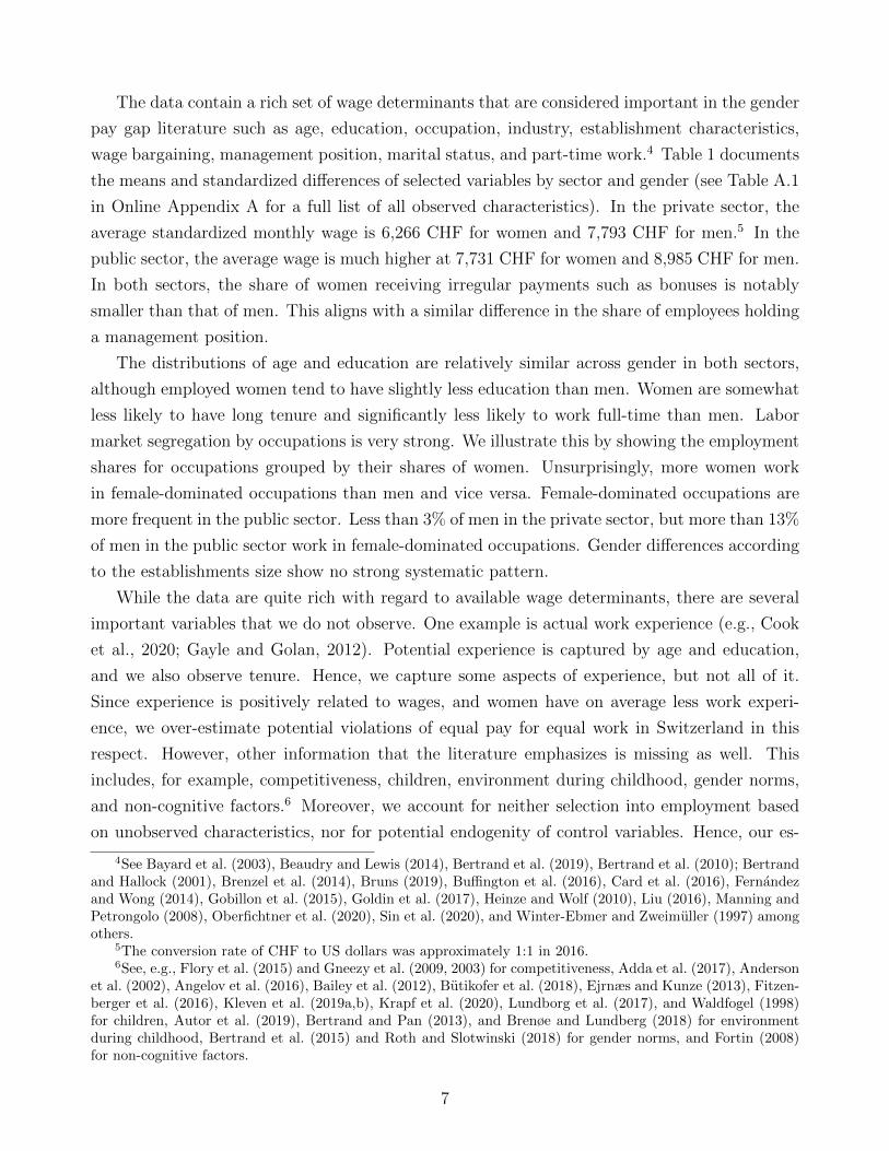
The data contain a rich set of wage determinants that are considered important in the gender

pay gap literature such as age, education, occupation, industry, establishment characteristics,

wage bargaining, management position, marital status, and part-time work.4 Table 1 documents

the means and standardized differences of selected variables by sector and gender (see Table A.1

in Online Appendix A for a full list of all observed characteristics). In the private sector, the

average standardized monthly wage is 6,266 CHF for women and 7,793 CHF for men.5 In the

public sector, the average wage is much higher at 7,731 CHF for women and 8,985 CHF for men.

In both sectors, the share of women receiving irregular payments such as bonuses is notably

smaller than that of men. This aligns with a similar difference in the share of employees holding

a management position.

The distributions of age and education are relatively similar across gender in both sectors,

although employed women tend to have slightly less education than men. Women are somewhat

less likely to have long tenure and significantly less likely to work full-time than men. Labor

market segregation by occupations is very strong. We illustrate this by showing the employment

shares for occupations grouped by their shares of women. Unsurprisingly, more women work

in female-dominated occupations than men and vice versa. Female-dominated occupations are

more frequent in the public sector. Less than 3% of men in the private sector, but more than 13%

of men in the public sector work in female-dominated occupations. Gender differences according

to the establishments size show no strong systematic pattern.

While the data are quite rich with regard to available wage determinants, there are several

important variables that we do not observe. One example is actual work experience (e.g., Cook

et al., 2020; Gayle and Golan, 2012). Potential experience is captured by age and education,

and we also observe tenure. Hence, we capture some aspects of experience, but not all of it.

Since experience is positively related to wages, and women have on average less work experi-

ence, we over-estimate potential violations of equal pay for equal work in Switzerland in this

respect. However, other information that the literature emphasizes is missing as well. This

includes, for example, competitiveness, children, environment during childhood, gender norms,

and non-cognitive factors.6 Moreover, we account for neither selection into employment based

on unobserved characteristics, nor for potential endogenity of control variables. Hence, our es-

4See Bayard et al. (2003), Beaudry and Lewis (2014), Bertrand et al. (2019), Bertrand et al. (2010); Bertrandand Hallock (2001), Brenzel et al. (2014), Bruns (2019), Buffington et al. (2016), Card et al. (2016), Fernandezand Wong (2014), Gobillon et al. (2015), Goldin et al. (2017), Heinze and Wolf (2010), Liu (2016), Manning andPetrongolo (2008), Oberfichtner et al. (2020), Sin et al. (2020), and Winter-Ebmer and Zweimuller (1997) amongothers.

5The conversion rate of CHF to US dollars was approximately 1:1 in 2016.6See, e.g., Flory et al. (2015) and Gneezy et al. (2009, 2003) for competitiveness, Adda et al. (2017), Anderson

et al. (2002), Angelov et al. (2016), Bailey et al. (2012), Butikofer et al. (2018), Ejrnæs and Kunze (2013), Fitzen-berger et al. (2016), Kleven et al. (2019a,b), Krapf et al. (2020), Lundborg et al. (2017), and Waldfogel (1998)for children, Autor et al. (2019), Bertrand and Pan (2013), and Brenøe and Lundberg (2018) for environmentduring childhood, Bertrand et al. (2015) and Roth and Slotwinski (2018) for gender norms, and Fortin (2008)for non-cognitive factors.

7

timates are informative about equal pay for equal work when individual choices are taken as a

given, subject to any omitted variable bias that may result from unobserved factors.

3 Econometric model and estimators

3.1 Notation and parameter of interest

We denote the gender dummy by Gi, with Gi = 1 for employed women and Gi = 0 for employed

men. We use the logarithm of the standardized monthly wage as the outcome variable, which

we denote by Yi. The raw gender pay gap is

∆ = E[Yi|Gi = 1]− E[Yi|Gi = 0]. (1)

The raw gender pay gap can be decomposed into an explained and unexplained part. The

vector Xi contains observed demographic and labor market characteristics of the employees

as well as observed characteristics of their employers. The predicted wage of employed men,

would they have the same observed characteristics as employed women is EX|G=1[µ0(x)], with

µ0(x) = E[Yi|Gi = 0, Xi = x]. Adding and subtracting EX|G=1[µ0(x)] in (1) gives

∆ = E[Yi|Gi = 1]− EX|G=1[µ0(x)]︸ ︷︷ ︸unexplained δ

+EX|G=1[µ0(x)]− E[Yi|Gi = 0]︸ ︷︷ ︸explained η

. (2)

The second difference on the right side of (2) is the part of the raw gender pay gap that can

be explained by gender differences in the observed wage determinants Xi. The first difference

on the right side of (2) is the gender pay gap for employed women that cannot be explained

by gender differences in the observed wage determinants. It is the expected difference in pay of

employed women compared to observationally identical employed men, which we denote by

δ = E[Yi|Gi = 1]− EX|G=1[µ0(x)]. (3)

This is the parameter of interest in the majority of studies on gender wage inequality.

3.2 Common support

The unexplained pay gap (3) is only identified if, for all females, there exist men that are

observationally identical with respect to the wage determinants. Now assume that there is lack

of support for some men or women. Let Si = 1 for individuals with support and Si = 0 for

8

individuals without support. Nopo (2008) shows that

∆ = E[Yi|Gi = 1, Si = 1]− E[Yi|Gi = 0, Si = 1]︸ ︷︷ ︸=∆S=1

+∆sG=1 −∆s

G=0

where ∆sG=g ≡ Pr(Si = 0|Gi = g)[E[Yi|Gi = g, Si = 0] − E[Yi|Gi = g, Si = 1]] measures wage

differences across individuals of gender g (for g ∈ {0, 1}) in and out of support. The parameter

∆S=1 is the raw wage gap within support, which we can decompose as

∆S=1 = E[Yi|Gi = 1, Si = 1]− EX|G=1,S=1[µ0(x)|Si = 1]︸ ︷︷ ︸δS=1

+EX|G=1,S=1[µ0(x)|Si = 1]− E[Yi|Gi = 0, Si = 1]︸ ︷︷ ︸ηS=1

.(4)

The first right-hand term, δS=1, is the unexplained gender pay gap for employed women with

support. The second right-hand term, ηS=1, is the part of the raw gender pay gap with support

that can be explained by gender differences in the wage determinants.

We use the following procedure to analyze the influence of common support violations on

gender pay gap estimates. First, we sequentially increase the number of wage determinants

for which we impose common support and then study the share of females without support.

Imposing common support based on a large number of wage determinants increases ex-ante

comparability of women and men. Second, we estimate the elements of (4) for each sequential

step using an exact matching estimator (see Section 3.3.4 for more details). Third, based on the

sequential analysis, we pick five exemplary definitions of support and estimate the unexplained

gender pay gap on support, δS=1. Specifically, we restrict the sample to the employees on support

and implement different estimators for the unexplained gender pay gap, which we explain in the

next section.

3.3 Estimators

There exists a very large set of possible parametric and semi-parametric estimators, doubly-

robust mixtures between the two types of estimators, and non-parametric estimators. We focus

on common estimators that are easy to implement with the objective of showing the main trade-

offs in estimator choice. We apply each estimator with five different support conditions where

we restrict the sample to the observations satisfying the respective support definition.

9

3.3.1 Dummy regression (LRM)

A simple estimation approach for the unexplained gender pay gap employs a linear regression

model (LRM) with a dummy for women,

Yi = α +GiδLRM +Xiβ + εi, (5)

where α is a constant, the vector β describes the association between the wage determinants

Xi and the wages, and εi is an error term. The parameter δLRM can be interpreted as the

unexplained gender pay gap.

The LRM imposes the restriction that the coefficients of the wage determinants as well

as the unexplained gender pay gap are homogeneous across all individuals. This includes the

assumption that the unexplained gender pay gap is equal for women and men. This modelling

assumption is unnecessarily restrictive, because it can be relaxed by including interaction terms

between gender and the wage determinants, which we discuss in the next section in the context

of the BO decomposition.

3.3.2 Blinder-Oaxaca (BO) decomposition

The BO decomposition is a two-step estimator that allows for heterogeneous unexplained gender

pay gaps (Blinder, 1973; Oaxaca, 1973). In the first step, we estimate in the subsample of men

the linear wage model

Yi = α0 +Xiβ0 + ui, (6)

where α0 is an intercept and ui is an error term. The coefficients β0 describe the association

between the wage determinants Xi and the wages of men. In the second step, we use the

estimated coefficients from this regression to predict the counterfactual male wage µ0(Xi) ≡α0 +Xiβ0 for each woman in the sample and estimate the mean unexplained gender pay gap for

women using

δBO =1

N1

N∑i=1

Gi(Yi − µ0(Xi)) (7)

with N1 =∑N

i=1Gi (hats indicate estimated parameters). Note that this estimation procedure

is numerically identical to using a linear prediction for female wages, Yi = α1 +Xiβ1 + vi, in the

sample of women and calculating the unexplained part of the pay gap as

δBO = (α1 − α0) +1

N1

N∑i=1

GiXi(β1 − β0),

10

since1

N1

N∑i=1

GiYi = α1 +1

N1

N∑i=1

GiXiβ1.

In contrast to the LRM, this version of the BO decomposition allows for gender differences in

the impact of characteristics Xi on wages as well as for heterogeneity in the unexplained gender

pay gap that is driven by these differences.

The BO model corresponds to the LRM augmented with interaction terms between gender

and all observable wage determinants:

Yi = α0 +Gi (α1 − α0)︸ ︷︷ ︸=αBO

+Xiβ0 +GiXi (β1 − β0)︸ ︷︷ ︸=βBO

+εi. (8)

Using this fully interacted LRM, we could estimate the BO unexplained wage gap by

δBO = αBO +1

N1

N∑i=1

GiXiβBO.

This estimation procedure is numerically identical to (7) when we control for the same charac-

teristics Xi as in (6).

3.3.3 Inverse probability weighting (IPW) estimators

Inverse probability weighting (IPW) estimators are also two-step estimators (Hirano et al., 2003;

Horvitz and Thompson, 1952). In the first step, we estimate the conditional probability of being

a women, the so-called propensity score, based on the model

p(Xi) = Pr(Gi = 1|Xi) = F (Xiγ),

where F (·) is a binary link function (e.g., the logistic distribution). In the second step, we

predict p(Xi) for all observations and estimate the re-weighted sample average

δIPW =1

N1

N∑i=1

GiYi −N∑i=1

W 0i Yi,

with the IPW weights

W 0i =

(1−Gi)p(Xi)

1− p(Xi)

/ N∑i=1

(1−Gi)p(Xi)

1− p(Xi)(9)

The denominator in (9) guarantees that the IPW weights add up to one in finite samples (see, e.g.,

Busso et al., 2014). In contrast to LRM and BO, IPW does not impose any specific functional

form on the relationship between Xi and the wage, and it does not restrict heterogeneity in

11

unexplained gender pay gaps. A potential disadvantage of IPW is its instability when the

conditional probability of being a women is close to one (e.g., Khan and Tamer, 2010), which

may results in high variance of δIPW . We impose trimming rules to avoid propensity score values

that are too extreme (see the discussion in, e.g., Lechner and Strittmatter, 2019). In particular,

we omit males with large weights p(Xi)/(1 − p(Xi)) above the 99.5% quantile.7 We document

the number of trimmed observations in Table B.1 of Online Appendix B.

Kline (2011) argues that BO estimators are equivalent to propensity score re-weighting es-

timators, but in contrast to IPW they model the propensity score linearly.8. As a result, the

implicit weights of BO can become negative, which is not possible for the IPW estimator. How-

ever, in the limit to a fully saturated BO model, even the linear specification of the propensity

score would be well behaved and negative weights would be unlikely.

Augmented inverse probability weighting (AIPW) dates back to Robins et al. (1994) and

has received significant attention since Chernozhukov et al. (2017) proposed this estimation

procedure in the context of machine learning. AIPW is a doubly-robust mixture between the

BO and IPW approach,

δAIPW =1

N1

N∑i=1

Gi(Yi − µ0(Xi))−N∑i=1

W 0i (Yi − µ0(Xi)), (10)

with µ0(Xi) as in BO. The first right-hand term in (10) is equivalent to the BO in (7). The second

right-hand term in (10) has an expected value of zero, but makes a finite sample adjustment by

re-weighting the observable bias of µ0(Xi) in the sample of men with the IPW weights.

AIPW is more robust to misspecification than BO or IPW. In particular, δAIPW is consistent

even when either µ0(x) or p(x) is misspecified. Moreover, the theoretical properties of AIPW

are well established for generic estimators of the nuisance parameters µ0(x) and p(x). In par-

ticular, 4√N -consistency of µ0(x) and p(x) is sufficient to achieve

√N -consistency of δAIPW (in

combination with the cross-fitting procedure described below). This permits the application of

flexible machine learning methods to estimate µ0(x) and p(x), which often have a convergence

rate below√N . AIPW combined with machine learning is often called double-machine-learning

(see Knaus, 2020, for a review).

3.3.4 Matching estimators

Exact matching (EXM) as used, for example by Nopo (2008), is a fully non-parametric estimation

approach. We stratify the sample into K � N mutually exclusive groups Wi ∈ {1, ..., K}, which

7We apply the normalization described in (9) after the trimming.8The usual practice of IPW estimators is to use a Logit or Probit estimator for the propensity score

12

are defined based on the characteristics Xi. The EXM estimator is

δEXM =1

N1

N∑i=1

Gi

Yi −N∑j=1

1{Wi = Wj}(1−Gj)YjN∑j=1

1{Wi = Wj}(1−Gj)

.

EXM is more flexible than LRM, BO, IPW and AIPW. However, it suffers from the curse of

dimensionality. When we consider many strata K, the risk of lacking support (i.e., finding no

men matching specific strata of women) increases. Unlike the previous estimators, EXM cannot

extrapolate into regions without support. Therefore, the estimation breaks down in the presence

of support violations. Furthermore, even when there is support, there may be strata with very

few men, which might lead to high variance of δEXM . Despite these potential disadvantages,

our large data set with more than one million observations remains suitable for EXM. However,

we have to define relatively coarse groups for the two continuous variables of age and tenure to

avoid empty strata. For the same reason, we have to combine some industries and occupations

with only few observations into more loosely similar groups. We implement EXM as in Nopo

(2008); i.e., we exactly match the stratified variables that define common support. This implies

that the versions with less restrictive support definitions also match on fewer variables, thus

removing fewer differences in observed wage determinants. In the private [public] sector, we

have 140 [142] strata for the least restrictive support definition and 844,100 [208,860] strata for

the most restrictive one.

We consider two additional semi-parametric matching estimators to account for potential

concerns regarding the curse of dimensionality and unmatched wage determinants within strata.

First, we use propensity score radius matching (PSM) (see e.g. Frolich, 2007; Lechner and Wun-

sch, 2009; Lechner et al., 2011). The propensity score p(Xi) is the same as for IPW. PSM is a

one-dimensional matching approach (as opposed to the multi-dimensional matching of EXM).

To each woman, we match the men who have a propensity score value within a certain absolute

difference (radius) of the woman’s propensity score value. We define the radius as the 99%

quantile of the distribution of the closest absolute distances for all women, then omit women

without a match within the radius. Table B.2 in Online Appendix B documents the number of

females we use for the different matching estimators. We lose only a relatively few women who

lack matching men within the defined radius.

Second, we consider mixtures between exact and propensity score radius matching (EXPSM).

Here, we exactly match on the wage determinants that define support, as in EXM, and apply

propensity score radius matching within each stratum using all wage determinants, as in PSM.

In contrast to EXM, the propensity score corrects semi-parametrically for remaining within-

13

strata observable differences between women and men. In contrast to PSM, we enforce exact

comparability of women and men with respect to some wage determinants.9

3.4 Flexibility of inclusion of wage determinants

To estimate the so-called nuisance parameters, i.e., the wage equation µ0(x) and the propensity

score p(x), we consider three different models. We call them the baseline, full, and machine

learning (ML) models. The baseline and full models include the same wage determinants, but we

vary the flexibility in terms of non-linear (e.g., polynomials, categorical dummies) and interaction

terms of the wage determinants. The ML model can select the relevant wage determinants and

the model flexibility in a data-driven way, using the full model specification as input. In practice,

it is often unclear which non-linear and interaction terms are relevant. Using a too parsimonious

model could bias δ, due to model misspecification. Allowing for too much flexibility could lead

to imprecise estimates of δ with high variance, especially in smaller samples. Accordingly, we

face a bias-variance trade-off.

3.4.1 Manual model specification

In the baseline model, we control for all observed variables in a standard way. Specifically, we in-

clude age (linear and squared), tenure (linear and squared), vocational education (9 categories),

citizen status (6 categories), marital status (3 categories), occupation (39 [20] categories in the

private [public] sector), industry sector (36 [12] categories in the private [public] sector), man-

agement position (5 categories [and a missing dummy for public sector]), region (7 categories),

establishment size (5 categories), and employment share as a fraction of full time (4 categories).

Furthermore, we control for the dummy variables of temporary employment, employment con-

tract with hourly wages, collective wage agreement, overtime hours payment, bonus payments

(e.g., from profit sharing), supplementary wages (e.g., for shift work), and extra salary (e.g.

Christmas and holiday salaries). Overall, the baseline model includes 117 control variables in

the specification for the private sector and 74 control variables in the specification for the public

sector.

In the full model, we add to the baseline model all non-linear and interaction terms that

we think could potentially be relevant. The non-linear terms are the polynomials of age and

tenure up to order seven, as well as four age and five tenure categories. Furthermore, we include

interaction terms between control variables to allow for heterogeneous returns to important wage

determinants.10 Specifically, we interact occupation and industry groups with the categorical

9It should be noted that we implement PSM after matching exactly on the three variables that define the leastrestrictive Support 1, because this improves matching without lack of support. As a result, PSM and EXPSMare identical for Support 1 but not for the other support definitions.

10We partially coarsen the categorical variables to improve support of the interaction terms.

14

variables for age, tenure, education, foreigner status, management position, and establishment

size. We also include interaction terms between establishment size categories and the categorical

variables for age, tenure, vocational education, migration, and management position. Finally,

we interact vocational education and management position categories with age and tenure cate-

gories. Overall, the full model includes 615 control variables in the specification for the private

sector and 396 control variables in the specification for the public sector.

3.4.2 Data-driven model specification

In contrast to manual model specification, machine learning estimators have the potential to

balance the bias-variance trade-off in a data-driven way. We use the LASSO to specify our ML

models. The LASSO is a penalized regression method (see Hastie et al., 2009, for a detailed de-

scription of the LASSO). It can balance the bias-variance trade-off by shrinking some coefficients

towards zero. Eventually, some covariates are excluded from the model when the coefficients

are exactly zero. Accordingly, the LASSO is a model selection device. To obtain the predicted

wages of men µ0(x) in the baseline and full models for BO, we estimate in the sample of men

the OLS model

(α0, β0) = arg mina,b

1

N

N∑i=1

(Yi − a−Xib)2,

and predict the conditional male wages by µ0(x) = α0 + xβ0. In contrast, the LASSO objective

function is

(α0, β0) = arg mina,b

1

N

N∑i=1

(Yi − a−Xib)2 + λ‖b‖1, (11)

with the penalty term λ‖b‖1 = λ∑P

p=1 |b|. The tuning parameter λ ≥ 0 specifies the degree

of penalization of the absolute coefficient size of β0. If λ = 0, the ML model is equivalent to

the full model. If λ > 0, some coefficients β0 shrink towards zero and eventually approach

zero exactly. Shrinking coefficients to zero is equivalent to excluding the corresponding control

variable in Xi from the wage equation. In the extreme case, when λ→∞, all coefficients in β0

are exactly zero and only the intercept α0 is non-zero, because it is not penalized. We determine

the tuning parameter λ with a 5-fold cross-validation procedure (Chetverikov et al., 2017).11

The cross-validation procedure selects the λ that minimises the mean-squared-error (MSE). To

smooth the ML model, we apply the one-standard-error rule to the minimum λ (see, e.g., Hastie

et al., 2009).

We use similar models to estimate the propensity score p(x). However, instead of using OLS,

we use the Logit estimator for the baseline and full model. Likewise, we use Logit-LASSO instead

11Alternatively, the choice of the tuning parameter λ can be based on information criteria (Zou et al., 2007)or data-driven procedures (Belloni et al., 2012).

15

of the standard LASSO approach for the ML model (see Hastie et al., 2016, for an introduction

to Logit-LASSO).12 In Figures C.1-C.8 in Online Appendix C, we report the density of the

estimated propensity scores by gender.

Post-double-selection (PDS) procedure. The LASSO version of the LRM corresponds

to the PDS procedure of Belloni et al. (2013, 2014). The conventional LASSO has the purpose of

predicting Yi, but it is not designed to obtain an unbiased estimate of the structural parameter

δLRM . To illustrate this, the application of LASSO to (5) without penalizing the gender dummy

would most likely lead to the omission of those wage determinants that are highly correlated with

gender, such that an omitted variable bias is inevitable. The PDS procedure enables LASSO

to select the relevant wage determinants in a data-driven way, without the threat of omitting

important variables. The PDS procedure has three steps. First, the LASSO selects the relevant

control variables in the linear wage equation Yi = αY + XiβY + νi, which does not contain the

the gender dummy Gi.13 In practice, the LASSO can set some coefficients in the vector βY to

zero, which is equivalent to excluding the corresponding control variables in Xi from the wage

equation. Second, the LASSO selects the relevant dimensions of Xi in the linear gender model

Gi = αG + XiβG + ηi. As before, the LASSO estimator can set some coefficients in the vector

βG to zero, such that only those control variables with a strongly gender correlation remain in

the model. We denote the union of all wage determinants with non-zero coefficients in either βY

or βG by Xi. Finally, we estimate the linear OLS model (called ’post-LASSO’)

Yi = αPDS +GiδPDS + XiβPDS + εi.

Belloni et al. (2013) show that the estimator of δPDS is consistent and asymptotically normal.

The PDS procedure allows for the inclusion of high-dimensional characteristics Xi (i.e., more

characteristics than observations), but requires Xi to be sparse. Some approximation error in the

selection of the Xi variables is permitted. The PDS procedure is doubly robust to misspecification

of either the earnings equation or the gender model.

For the same reason as for the LRM, applying LASSO in a naive way to the interacted BO

in (8) could lead to biased estimates of αBO and βBO, which could also bias δBO. However,

we can use the LASSO to estimate µ0(x), since µ0(x) is a pure prediction model for Yi, and

then use µ0(x) as a plug-in estimator in (7). Accordingly, (7) provides a way to combine the

Blinder-Oaxaca decomposition with standard machine learning methods. This procedure is

called T-learner in the denomination of Kunzel et al. (2019). A possible disadvantage of this

approach is that we do not obtain estimates of the parameters αBO and βBO, since they are

not required to estimate δBO. Alternatively, Bach et al. (2018) propose a procedure that is

12The only exception is the post-double-selection procedure, for which we use a linear model to estimate thepropensity score, as proposed in Belloni et al. (2013).

13In contrast to (11), we use the sample of men and women for the wage equation of the PDS procedure.

16

based on post-double-selection, but is more flexible and allows us to obtain estimates of selected

parameters in αBO and βBO.

Cross-fitting. To avoid over-fitting and obtain√N convergence for AIPW, it is necessary to

estimate the ML models of µ0(x) and p(x) in a different sample than δAIPW (see Chernozhukov

et al., 2018b). We achieve this by using cross-fitting. We partition the sample into two parts of

equal size. We estimate µ0(x) and p(x) with the first partition, extrapolate their fitted values

to the second partition and use these values to estimate δAIPW . Thereafter, we switch the first

and second partition and repeat the procedure, such that the entire data set is used efficiently.

We report the average δAIPW across both partitions.

Selected variables. We allow the LASSO to select among all control variables of the full

model. Table C.1 in Online Appendix C documents the number of selected control variables for

all ML models we consider. The final specifications vary by support and estimation procedure.

For the wage equation, the ML model considers between 371 and 513 control variables in the

different specifications for the private sector and between 215 and 306 control variables for the

public sector. For the propensity score model, the ML model considers between 141 and 428

control variables for the private sector and between 126 and 230 control variables for the public

sector.

Performance. In Tables C.2 and C.3 in Online Appendix C, we report the out-of-sample

prediction power of the different nuisance parameter models. To obtain the out-of-sample predic-

tion power, we use a cross-fitting procedure.14 The prediction power of the baseline, full, and ML

models does not differ strongly. Accordingly, the baseline model already explains a significant

amount of the variation in the data. The prediction power of the full model is systematically

better than the prediction power of the baseline model, but the additional gain is moderate. The

ML model cannot systematically outperform the full model. The prediction power of the full

and ML models is fairly similar, even though the ML model controls for many fewer variables

than the full model. This suggests that the full model is too flexible. However, because of our

large data set, the prediction power of the full model does not deteriorate compared to the ML

model. The degrees of freedom loss of the full compared to the ML model appear to be of minor

importance. However, we expect that the ML model would outperform the full model in smaller

samples.

14We partition the data in two equally sized samples, using one partition as a training sample and the otheras a test sample. Thereafter, we switch the two partitions and report the average prediction power across thetwo samples.

17

4 Results

4.1 Analysis of common support

Our first step is to analyze common support using the approach of Nopo (2008). We sequentially

increase the number of wage determinants for which we impose common support. To determine

the order in which we add variables, we run a simple wage regression in the sample of men, i.e. we

estimate µ0(x) in order to determine the importance of the different variables for explaining men’s

wages. We measure importance as the change in adjusted R2 when we omit one block of variables,

e.g. all occupation dummies, but keep all other wage determinants. We do this separately for

the private and public sectors and sort all variable blocks in decreasing order according to the

average R2 changes across both sectors. Thus, we start with the most important variable block

for explaining male wages and finish with the least important. We report the resulting order

of variables and the sector-specific changes in the adjusted R2 in Tables B.3 and B.4 of Online

Appendix B for the private and public sector, respectively.

Our choice of ordering based on importance for explaining male wages is motivated by the

curse of dimensionality. The larger the number of variables with respect to which we enforce

common support, the more likely it is that there will be empty cells. As a result, we expect

the share of the original sample for which there is support to decrease as we add more and

more variables. This implies that there is some difficulty in achieving a reasonable balance of

comparability, sample size and representativeness of the remaining sample. Therefore, we want

to impose support with respect to variables that significantly influence the counterfactual male

wage, but not necessarily with respect to variables of minor importance.

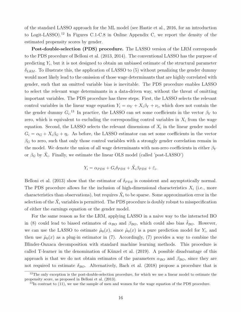
In Figure 1, we report how the share of women with support falls as we increase the number

of wage determinants with respect to which we enforce support. There is full support with

respect to the three most important determinants – management position, education and age

– in the private sector, and only 2 women are off support in the public sector. The loss of

observations due to lack of support is relatively small when we add industry and occupation,

which are both highly relevant for predicting wages. It becomes larger but remains below 20%

if we add establishment size and a dummy for irregular payments. Thereafter, however, support

deteriorates quickly. Once we enforce support with respect to the 10 variables that are most

important for explaining male wages, 55% of women in the private sector and 32% of women in

the public sector have no comparable men with respect to these variables. The loss of women is

stronger in the private sector than in the public sector because the latter is more homogeneous in

terms of occupations and industries. Subsequently adding the less important wage determinants

further reduces support, resulting in lack of support for 89% of women in the private sector and

70% of women in the public sector when we enforce full support with respect to all observed

wage determinants.

18

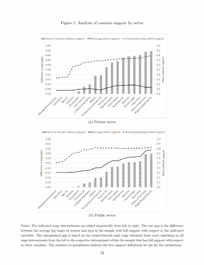
Figure 1: Analysis of common support by sector

(a) Private sector

(b) Public sector

Notes: The indicated wage determinants are added sequentially from left to right. The raw gap is the difference

between the average log wages of women and men in the sample with full support with respect to the indicated

variables. The unexplained gap is based on the counterfactual male wage obtained from exact matching on all

wage determinants from the left to the respective determinant within the sample that has full support with respect

to these variables. The numbers in parentheses indicate the five support definitions we use for the estimations.

19

Of course, different orders of variables lead to different evolutions of support. Table B.5 in

Online Appendix B shows how support changes when we add these variables in three alternative

orders. The first one uses sector-specific R2 changes rather than the average over both sectors

to order variables. For the main analysis, we want to keep the results comparable across sectors,

which is why we want the same order for both sectors. The order resulting from sector-specific

R2 changes differs across sectors for some variables, but the overall differences are moderate. Ac-

cordingly, the evolution of support when adding variables is also similar. The second alternative

is a random order. Here support remains higher for a larger number of added variables, mainly

because critical variables such as industry and tenure are, by chance, added relatively late. This

would change with a different random order in which the are added earlier. The last alternative

uses an increasing order according to the sector-average R2 changes as the other extreme to

a decreasing order. Here, support breaks down rather late. The reasons for this are twofold.

First, the ordering prioritizes wage determinants in which women and men do not greatly differ.

Second, many of these wage determinants are dummies while more important variables (such

as education, occupation and industry) have many different categories. This mechanically splits

the sample in more cells than a dummy variable such that cell size is reduced.

Besides studying the evolution of support, we also estimate the elements of (4). The raw

gender pay gaps on support, ∆S=1 , can be obtained from the average gender difference in wages

in the sample with support. To estimate the unexplained gender pay gap for the women with

support, δS=1, we follow Nopo (2008) and calculate the pay gap that remains after matching

exactly on all variables for which we enforce support. Thus, when adding support-relevant

wage determinants, we also increase the number of variables on which we exactly match. The

explained gender pay gap on support, ηS=1, can be calculated as the difference between the raw

and unexplained gender pay gap within support. We report the main insights from this analysis

in Figure 1 and we document the full set of results in Tables B.3 and B.4 in Online Appendix

B.

The raw gender pay gap is relatively insensitive to the support definition in the private

sector. It decreases only slightly, from 18.6% under the weakest support definition to 17.3%

under the strongest one. In contrast, the EXM estimates of the unexplained and explained

gender pay gaps are very sensitive to the support definition. The unexplained gender pay gap

on support falls from 13.4% under the weakest support definition to 4.2% under the strongest

one. Correspondingly, the explained gender pay gap increases from 5.1% to 13.1% as we exactly

match on more wage determinants. Interestingly, the results differ substantially for the public

sector. Here, a substantial part of the raw gender pay gap is due to women without support.

The raw gender pay gap on support decreases from 13.9% under the weakest support definition

to only 4.5% under the strongest one. The unexplained gender pay gap on support decreases

quickly from 9.7% to to 3.5% when we impose support with respect to, and exactly match on, the

20

eight most important wage determinants. Thereafter, imposing stronger support and matching

on more variables leaves the unexplained gender pay gap almost unchanged although the raw

gender pay gap decreases. This finding is in line with strongly regulated wage setting of the

Swiss public sector, which leaves little room for gender pay differences.

For the analysis of the unexplained gender pay gap with different estimation methods and

model flexibility, we pick five definitions of support that illustrate the trade-offs between com-

parability, sample size and representativeness. We indicate the five versions with the respective

number in parentheses in Figure 1. Here it is important to note that for a given choice of variables

it does not matter in which order support is enforced. All possible orders will lead to exactly

the same sample. Support 1 does not change the sample except for excluding two women in

the public sector. Thus, it effectively resembles the case without support enforcement. Support

2 enforces support with respect to classical and very important wage determinants. Support 3

covers all quantitatively important wage determinants. Support 4 adds tenure as the only proxy

for actual experience, but it does not significantly explain wages. Support 5 is the most extreme

case, which enforces full support with respect to all variables. Table B.6 in Online Appendix B

shows how imposing stricter support changes the average characteristics of the remaining women

with support. The changes are largest with respect to occupation, management position, estab-

lishment size, and part-time employment status. This is important for the interpretation of our

results. In the presence of heterogeneous pay gaps, we cannot expect estimates to be the same

when the sample changes due to stricter enforcement of support.

4.2 Analysis of the unexplained gender pay gap

In panels (a), (c) and (e) of Figures 2 and 3, we show the estimates of the average unexplained

gender pay gap for the private and public sector, respectively. The bars show the unexplained

gender pay gap estimates of the different methodological choices we consider and the capped

lines show the 95% confidence interval for each estimate.15 As a benchmark, the black horizontal

line shows the BO estimate in Support 1 (full sample except for two women in the public sector)

with the baseline specification together with its 95% confidence interval (black dashed lines).

Furthermore, panels (b), (d) and (f) of both figures show the percentage differences of each

estimate from this benchmark.

We find that all of the methodological choices we consider matter greatly. Compared to the

BO benchmark, using a less flexible estimator like the LRM increases the estimated unexplained

gender pay gap by up to 29%. In contrast, increasing flexibility by including wage determinants

more flexibly or by using a more flexible estimator together with enforcing common support

15We do not include exact matching (EXM) as EXM does not control for all wage determinants in Supports(1)-(4), but EXM has already been discussed in the context of Figure 1. Tables D.1 and D.2 in Online AppendixD report all estimates including EXM with their standard error for the private and public sector, respectively.

21

Figure 2: Mean unexplained gender pay gap in the private sector

(a) Baseline model: estimates (b) Baseline model: difference to benchmark

(c) Full model: estimates (d) Full model: difference to benchmark

(e) ML model: estimates (f) ML model: difference to benchmark

Notes: We report all estimates and their standard errors in Table D.1 in Online Appendix D. Capped lines

indicate the 95% confidence intervals of the estimated unexplained gender pay gap. The black horizontal line in

the left panels shows the BO estimate of Support 1 as a benchmark with the baseline specification and its 95%

confidence band in black dashed lines. The right panels show the difference from this benchmark in percent, i.e.,

the difference from the BO estimate using Support 1 with baseline model specification. PDS is the abbreviation

for post-double-selection procedure.

22

Figure 3: Mean unexplained gender pay gap in the public sector

(a) Baseline model: estimates (b) Baseline model: difference to benchmark

(c) Full model: estimates (d) Full model: difference to benchmark

(e) ML model: estimates (f) ML model: difference to benchmark

Notes: We report all estimates and their standard errors in Table D.2 in Online Appendix D. Capped lines

indicate the 95% confidence intervals of the estimated unexplained gender pay gap. The black horizontal line in

the left panels shows the BO estimate of Support 1 as a benchmark with the baseline specification and its 95%

confidence band in black dashed lines. The right panels show the difference from this benchmark in percent, i.e.,

the difference from the BO estimate using Support 1 with baseline model specification. PDS is the abbreviation

for post-double-selection procedure.

23

reduces the estimated pay gap by up to 50%. These differences are substantial. In the follow-

ing section, we investigate the role of each methodological choices separately: enforcement of

common support, flexibility in the inclusion of wage determinants, and estimator choice.

4.2.1 Role of stricter support enforcement

Figure 4 shows the differences in the estimated unexplained gender pay gaps for each support

definition relative to Support 1. We report separate results for each estimator, but pool the

results for the different model specifications (baseline, full, ML) for a better overview.

Figure 4: Difference in estimated unexplained gender pay gap relative to Support 1

Notes: Difference in percent to the estimate for Support 1 using the respective estimator. The results for the

model specifications (baseline, full, ML) are pooled.

The estimated pay gaps shrink substantially and, with few unsystematic exceptions, mono-

tonically with stricter support enforcement. For the BO estimates, enforcing support with

respect to all quantitatively important wage determinants (Support 3) reduces the estimated

pay gap by around 6% in both sectors, while enforcing full support with respect to all variables

(Support 5) reduces estimated gaps by around 26%. With 13-35% for Support 3 and 5-50% for

Support 5, the differences are considerably larger for the semi-parametric estimators IPW, PSM

and EXPSM. Overall, enforcing common support has a very strong impact on the size of the

estimated unexplained gender pay gaps.

There are two possible explanations for this finding. First, stricter support enforcement

makes women and men more comparable. Hence, differences in observed wage determinants

are likely to explain a larger share of the raw gender pay gap. This is particularly true for the

public sector, where a large part of the raw gender pay gap can be explained by lack of support

directly (see Figure 1). Second, heterogeneity in unexplained gender pay gaps can explain the

differences across support samples that differ increasingly in their composition (see Table B.6 in

24

Online Appendix B). For example, stricter support enforcement increasingly removes women in

lower-paying jobs. As a result, the unexplained gender pay gap could either increase or decrease,

depending on whether the unexplained gender pay gap is larger for women in higher- or lower-

paying jobs. However, the direction cannot be inferred from data, because we cannot estimate

the unexplained gender pay gap for the omitted women who lack comparable men.

The results are consistent with the findings of Nopo (2008), who shows that 11% of Peru’s

gender pay gap estimates can be explained by lack of common support with regard to age,

education, marital status, and migration condition. We document that support violations can

be much more severe when accounting for a richer set of wage determinants. Furthermore, we

show that all estimators are affected by support violations, including the parametric estimators

that rely on extrapolation.

4.2.2 Role of model flexibility

Controlling for wage determinants more flexibly is also important, especially for the parametric

estimators. Figure 5 shows the percentage differences in the estimated unexplained gender

pay gaps between the baseline model of the respective estimator and the full and ML model

specifications. We report separate results for each estimator, but pool the results of the different

support definitions for a better overview.

Figure 5: Difference in estimated unexplained gender pay gap relative to baseline model

Notes: Difference in percent of the baseline model estimate with the respective estimator. The results for the

different support definitions are pooled.

We find that the most flexible full model specification reduces the BO estimate of the pay

gap by 6% in the private sector and 19% in the public sector. The reductions are only slightly

smaller for the ML specification, which selects variables from the full model in a data-driven

way to increase efficiency.

25

Model flexibility matters most for the parametric estimators LRM and BO; as well as for

AIPW, which can be viewed as an extension of BO with semi-parametric small-sample bias

adjustment. All three estimators model the wage equation to estimate the unexplained gender

pay gap. In contrast, the semi-parametric estimators IPW, PSM and EXPSM are much less

sensitive to how wage determinants are included. All three estimators only use the propensity

score as an input factor and do not impose any functional form on the wage equation. For

those estimators, the estimated pay gaps differ by less than 8% from the baseline model. The

most flexible one, EXPSM, exhibits only very small differences across model specifications: only

0.4% in the private sector and 3% in the public. For all estimators, the difference between the

full and ML models are not very large. A noticeable exception is the IPW estimator, where

the unexplained gender pay gap of the ML specification exceeds even the baseline specification.

Knaus et al. (2020) document low finite sample performance of IPW in combination with ML,

which may explain this result.

Kline (2011) provides a theoretical justification for the sensitivity of the BO estimator with

regard to model flexibility. He argues that BO is more vulnerable to model misspecification

than IPW, because the implicit weighting scheme of BO allows for negative weights (which is

not permitted for IPW). When the BO model is specified more flexibly, though, negative implicit

weights become less likely.

We draw three conclusions from these results. First, controlling for wage determinants in a

flexible way is important. Second, the more flexibly they are included, the better; misspecifi-

cation of functional forms is less likely and the loss of degrees of freedom is not costly in our

very large data set (but this might be different in smaller data sets). Third, flexible inclusion

of wage determinants is more important for the estimators that incorporate the wage equation

than for estimators that only incorporate the propensity score. With our very large database,

we also find that applying machine learning methods for variable selection from a very rich set

of non-linear and interaction terms has only a small impact on the estimated pay gaps. This

may be different, though, in smaller samples where efficiency is more of a concern.

4.2.3 Role of estimator choice

The last dimension we vary is estimator choice. Figure 6 shows the differences in the estimated

unexplained gender pay gaps between BO and the respective estimator for each support. As the

flexibility of including wage determinants affects the parametric and semi-parametric estimators

differently, we focus on the results from the full model with maximum flexibility for all estimators.

This implies that the differences that we observe across estimators mainly result from differences

in the way the estimators restrict possible heterogeneity in unexplained gender pay gaps. The

LRM imposes homogeneous gender pay gaps. BO allows for heterogeneous gender pay gaps that

are driven by gender differences in the returns to the included wage determinants. In contrast,

26

the semi-parametric estimators IPW, PSM and EXPSM do not restrict heterogeneity in the pay

gaps at all. AIPW is a mixture between the parametric BO and a small sample bias adjustment

based on the the semi-parametric IPW. With our very large samples, small-sample bias should

be negligible and BO and AIPW should yield very similar results.

Figure 6: Difference in estimated unexplained gender pay gap relative to BO in respectivesupport

Notes: Difference in percent of the BO estimate in the respective support sample. All estimates are for the full

model, which is the most flexible specification.

We find that for each support, LRM estimates of pay gaps are 8-18% higher than the BO

estimate. The differences between the estimated BO and AIPW pay gaps are small as expected

with our large samples. This may be different in smaller samples, though. For the matching

estimators PSM and EXPSM we estimate pay gaps that are systematically and substantially

smaller than the corresponding BO estimates on the same support by up to 20% in the private

and up to 34% in the public sector. This is in line with substantial heterogeneity in estimated

pay gaps that is widely acknowledged in the literature (e.g. Bach et al., 2018; Chernozhukov et

al., 2018a; Goldin, 2014).

However, we find no systematic pattern for IPW. In the private sector, we find estimates

smaller than with BO and similar to PSM and EXPSM for supports 1-4, but much larger

estimates for support 5. In the public sector, we obtain estimates that are 5-24% larger than the

BO estimates for supports 1-4 and much smaller for full support 5. The results for IPW show

that this estimator is very sensitive to the population studied.

We conclude that it is important not to restrict pay gap heterogeneity by using a semi-

parametric estimator. Moreover, among the semi-parametric estimators, PSM and EXPSM

are much more robust and precise. The differences between PSM and EXPSM are small in

most cases. With a sufficient numbers of observations, EXPSM is preferable because it ensures

comparability of women and men in the best way among all considered estimators. Moreover,

27

EXPSM is the least sensitive to the way we include the observed wage determinants because

exact matching on the variables that define support fully removes all differences in these variables

without imposing any restrictions.

These findings are consistent with the results of Frolich (2007), who documents that the

PSM estimates of the unexplained gender pay gap in the UK are up to 29% smaller than the

BO estimates. Black et al. (2008) also find strong differences between BO and EXM estimates

of the unexplained gender pay gap in the United States. In particular, the estimates decline by

18% for white women, 92% for Hispanic women, and 83% for Asian women. However, for black

women they find no strong difference between the BO and EXM estimates. Likewise, Nopo

(2008) and Goraus et al. (2017) find no strong differences in the BO and EXM estimates of the

unexplained gender pay gap in Peru and Poland, respectively, but they only account for a very

small set of wage determinants. In Figure 1, we show that the selection of control variables is

crucial for EXM.

5 Discussion

5.1 Relevance of the Swiss case

A legitimate question is whether the results we obtain with the Swiss data are relevant for other

applications. In terms of data, ours are very similar to those of the European Union Structure of

Earnings Survey (SES). The SES provides harmonized data on earnings in EU member states,

candidate countries, and EFTA countries. It includes all of the wage determinants that have

been used to define Supports 1-4 (but not 5), which covers all quantitatively important wage

determinants. Moreover, like the Swiss data, actual work experience is not included. Studies

for the US typically use survey data collected from individuals such as the Current Population

Survey (CPS), the US Census, or the American Community Survey (ACS). Such surveys contain

much richer information on individuals but potentially suffer from measurement error in self-

reported wages. However, the key wage determinants we observe are included as well, and most

studies use a similar set of variables. In terms of sample size, all of the data sets are also very

large, containing several hundred thousand observations.

With respect to labor market institutions, Switzerland is a particularly interesting case. On

the one hand, it has generous social insurance systems like many other European countries. On

the other hand, it has a very flexible labor market that is much less regulated than that of other

European countries, which makes it more comparable to countries like the US. Thus, Switzerland

shares important features of both typically European labor markets and flexible US-type labor

markets. The differences we find between the private and the public sectors in Switzerland are

also likely to be relevant for other countries. Public sectors in most countries share the features

28

that explain the differences in the Swiss case. They are are typically more homogeneous in

terms of covered occupations with strong concentration in certain service sectors, they typically

attract a higher share of women than the private sector, they exhibit higher shares of high-skilled

workers, and they are typically more regulated, including their wage setting, than private sectors

(see Brindusa et al., 2012).

In summary, the data and labor market institutions in Switzerland are in many ways com-

parable to those in other countries. Therefore, we expect that our qualitative results extend

to other settings as well. Of course, the magnitudes of gender pay gaps differ greatly across

countries (see e.g. Weichselbaumer and Winter-Ebmer, 2005; Van der Velde et al., 2015). Hence,

we also expect the quantitative impact of methodological choices to differ. However, given that

most countries share key features of female employment and gender segregation in the labor mar-

ket, we are confident that the methodological choices we study are relevant beyond the Swiss

context.

5.2 Implications for applied research

Our results suggest that deciding how to enforce common support is the first important choice

in applied research about the gender pay gap. Researchers face a trade-off between stricter

support to improve ex-ante comparability, and sample size. The latter affects both the precision

of the estimate and the representativeness of the study sample. We recommend starting with an

analysis of common support using the approach of Nopo (2008), adding variables in decreasing

order of their impact on counterfactual male wages. Based on this analysis, there are two

possible criteria for choosing the set of variables for enforcing support. One option is to use all

quantitatively important wage determinants. In our application, this would result in support

definition 3 with 39% of employed women lost in the private sector and 20% lost in the public

sector, which is quite substantial. Alternatively, one could base the decision on the importance

of wage determinants for explaining the raw gender pay gap rather than the counterfactual male

wage. In this case, the researcher could choose the point at which the unexplained gender pay

gap obtained from exact matching stabilizes. In our data, this is the case somewhere between

Supports 2 and 3 (see Figure 1). As sample size drops considerably after enforcement of Support

2 plus irregular payments, this would be a natural choice of the set of variables for enforcing

support. This would exclude 19% of employed women in the private sector and 10% in the public

sector with the composition of the study sample being quite similar to that of the full sample.

The next important decision is which estimator to use. The results indicate that restricting

how observed wage determinants and gender may affect wages can have a large impact on the

estimated unexplained gender pay gap. When using BO, including wage determinants in a

flexible way is crucial. However, with a sufficiently large sample, a flexible matching estimator is

even better, as matching does not restrict gender pay gap heterogeneity in any way. The results

29

suggest that combining exact matching on few very important wage determinants that also

define support with radius matching on a flexibly specified propensity score works particularly

well. It minimizes the risk of functional form misspecification and, with support defined as

described in the last paragraph, offers a good balance between ensuring comparability, precision

and representativeness of the study sample.

Implementing these recommendations with our data would affect the estimated unexplained

gender pay gap in the following way. Consider Support 3 as the more conservative of the two

alternatives discussed above. In the private sector, enforcing Support 3 reduces the raw gender

pay gap of 18.6% by only 1%. Standard BO with the baseline specification for including wage

determinants that ignores support explains 58% of the raw gap in the full sample and results in

an estimate of the unexplained pay gap of 7.7%. Enforcing Support 3 reduces this estimate by

5%, using the most flexible instead of the baseline specification for BO by another 5%, and using

semi-parametric EXPSM with the same flexible specification instead by another 13%. In total,

the methodological choices decline the unexplained gender pay gap estimates by 23%. Flexible

EXPSM yields an estimated unexplained gap of 6% and explains 68% of the raw wage.

The differences are even larger for the public sector. Enforcing Support 3 already reduces

the raw gender pay gap of 13.9% by 14%. Standard BO without support enforcement explains

54% of the raw gap in the full sample and yields an estimate of the unexplained pay gap of

6.4%. Enforcing Support 3 reduces this estimate by 4%. Using the most flexible instead of the

baseline specification for BO has a strong impact, as it reduces the estimate by another 19%.

Using semi-parametric EXPSM with the same flexible specification instead leads to another even

more substantial reduction of 26%. In total, the methodological choices decline the estimates of

the unexplained gender pay gap by 50%. Flexible EXPSM yields an estimated unexplained gap

of only 3.2% and explains 77% of the raw wage. This once again illustrates the importance of

these methodological choices.

6 Conclusion

We study the sensitivity of estimates of the unexplained gender pay gap to three types of

methodological choices: enforcement of comparability of men and women ex ante, flexibility in

the inclusion of wage determinants, and choice of estimator. We find that all of these choices

matter greatly. Implementing the choices we recommended based on our results using data for

the Swiss private sector, explains 16% more of the raw wage gap than standard BO estimates

and results in estimated unexplained pay gaps that are 23% lower. For the public sector, the

preferred set of choices explains 42% more of the raw wage gap than standard BO estimates and

results in estimated unexplained pay gaps that are 50% lower.

An important takeaway from our study is that the commonly reported Blinder-Oaxaca es-

30

timates of the unexplained gender pay gap can be misleading for several reasons. There is a

high risk that they compare women to non-comparable men to an extent that is quantitatively

important. Moreover, they hide gender inequalities that result from this lack of comparability.

For females with lack of support, we know nothing about possible inequalities in pay. Moreover,

lack of support shows the extent of labor market segregation as an additional source of gender

inequality. This is ignored if researchers do not check for common support. More generally, the

restrictions standard BO imposes bear a high risk of yielding biased estimates of the unexplained

gender pay gap. In particular, they underestimate the full extent of heterogeneity in pay gaps

that is important for targeting affirmative action campaigns. Future work should study this

heterogeneity in more detail.

As a final remark, we would like to emphasize that our findings provide guidance on how

to estimate unexplained gender pay gaps with a given set of observed wage determinants. The

results from such estimations are informative about equal pay for equal work taking individ-

ual choices as a given, subject to any omitted variable bias that may result from unobserved

factors. Actual experience, having children, and personality traits are examples of such unob-

served factors in the data we have used. Uncovering the extent and sources of possible gender

discrimination in the labor market requires much more than accounting for unobserved wage

determinants, though, such as dealing with selection into employment and endogenous control

variables.

31

References

Adda, J., C. Dustmann, and K. Stevens, “The Career Costs of Children,” Journal of

Political Economy, 2017, 125(2), 293–337.

Anderson, D.J., M. Binder, and K. Krause, “The Motherhood Wage Penalty: Which

Mothers Pay It and Why?,” American Economic Review, 2002, 92(2), 354–358.

Angelov, N., P. Johansson, and E. Lindahl, “Parenthood and the Gender Gap in Pay,”

Journal of Labor Economics, 2016, 34(3), 545–579.

Autor, D., D. Figlio, K. Karbownik, J. Roth, and M. Wasserman, “Family Disad-

vantage and the Gender Gap in Behavioral and Educational Outcomes,” American Economic

Journal: Applied Economics, 2019, 11(3), 338–381.

Bach, P., V. Chernozhukov, and M. Spindler, “Closing the U.S. Gender Wage Gap Re-

quires Understanding its Heterogeneity,” arXiv:1812.04345, 2018.

Bailey, M.J., B. Hershbein, and A.R. Miller, “The Opt-In Revolution? Contraception

and the Gender Gap in Wages,” American Economic Journal: Applied Economics, 2012,

4(3), 225–254.

Baron, J.D. and D.A. Cobb-Clark, “Occupational Segregation and the Gender Wage Gap

in Private- and Public-Sector Employment: A Distributional Analysis,” Economic Record,

2010, 86(273), 227–246.

Barsky, R., J. Bound, K. Charles, and J. Lupton, “Accounting for the Black-White

Wealth Gap: A Nonparametric Approach,” Journal of the American Statistical Association,

2002, 97, 663–673.

Bayard, K., J. Hellerstein, D. Neumark, and K. Troske, “New Evidence on Sex Seg-

regation and Sex Differences in Wages from Matched Employer-Employee Data,” Journal of

Labor Economics, 2003, 21 (4), 887–922.

Beaudry, P. and E. Lewis, “Do Male-Female Wage Differentials Reflect Differences in the

Return to Skill? Cross-City Evidence from 1980-2000,” American Economic Journal: Applied

Economics, 2014, 6(2), 178–194.

Belloni, A., D. Chen, V. Chernozhukov, and C. Hansen, “Sparse Models and Methods for

Optimal Instruments With an Application to Eminent Domain,” Econometrica, 2012, 80(6),

2369–2429.

32

, V. Chernozhukov, and C. Hansen, “Inference on Treatment Effects After Selection

Amongst High-Dimensional Controls (with an Application to Abortion and Crime),” Review

of Economic Studies, 2013, 81(2), 608–650.

, , and , “High-Dimensional Methods and Inference on Treatment and Structural Effects

in Economics,” Journal of Economic Perspectives, 2014, 28(2), 29–50.

Bertrand, M. and J. Pan, “The Trouble with Boys: Social Influences and the Gender Gap in

Disruptive Behavior,” American Economic Journal: Applied Economics, 2013, 5(1), 32–64.

and K.F. Hallock, “The Gender Gap in Top Corporate Jobs,” ILR Review, 2001, 55(1),

3–21.

, C. Goldin, and L.F. Katz, “Dynamics of the Gender Gap for Young Professionals in the

Financial and Corporate Sectors,” Review of Economic Studies, 2010, 2(3), 228–255.

, E. Kamenica, and J. Pan, “Gender Identity and Relative Income within Households,”

Quarterly Journal of Economics, 2015, 130(2), 571–614.

, S.E. Black, S. Jensen, and A. Lleras-Muney, “Breaking the Glass Ceiling? The

Effect of Board Quotas on Female Labour Market Outcomes in Norway,” Review of Economic

Studies, 2019, 86(1), 191–239.

Black, D.A., A. Haviland, S.G. Sanders, and L.J. Taylor, “Gender Wage Disparities

among the Highly Educated,” Journal of Human Resources, 2008, 43(3), 630–659.

Blau, F.D. and L.M. Kahn, “Gender Differences in Pay,” Journal of Economic Perspectives,

2000, 14(4), 75–99.

and , “The Gender Wage Gap: Extent, Trends, and Explanations,” Journal of Economic

Literature, 2017, 55(3), 789–865.

Blinder, A., “Wage Disrimination: Reduced Form and Structural Estimates,” Journal of Hu-

man Ressources, 1973, 8(4), 436–455.

Bonjour, D. and M. Gerfin, “The Unequal Distribution of Unequal Pay – An Empirical

Analysis of the Gender Wage Gap in Switzerland,” Empirical Economics, 2001, 26(2), 407–427.

Brenøe, A.A. and S. Lundberg, “Gender Gaps in the Effects of Childhood Family Environ-

ment: Do they Persist into Adulthood?,” European Economic Review, 2018, 109, 32–62.

Brenzel, H., H. Gartner, and C. Schnabel, “Wage Bargaining or Wage Posting? Evidence

from the Employers’ Side,” Labour Economics, 2014, 29, 41–48.

33

Briel, S. and M. Topfer, “The Gender Pay Gap Revisited: Does Machine Learning offer New

Insights?,” Working Paper, 2020.

Brindusa, A., S. de la Rica, and J.J. Dolado, “The Effect of Public Sector Employment

on Women’s Labour Market Outcomes,” Washington, DC: World Bank, 2012.

Bruns, B., “Changes in Workplace Heterogeneity and How They Widen the Gender Wage

Gap,” American Economic Journal: Applied Economics, 2019, 11(2), 74–113.

Buffington, C., B. Cerf, C. Jones, and B.A. Weinberg, “STEM Training and Early

Career Outcomes of Female and Male Graduate Students: Evidence from UMETRICS Data

Linked to the 2010 Census,” American Economic Review, 2016, 106(5), 333–338.

Busso, M., J. DiNardo, and J. McCrary, “New Evidence on the Finite Sample Properties of

Propensity Score Reweighting and Matching Estimators,” Review of Economics and Statistics,

2014, 96(5), 885–897.

Butikofer, A., S. Jensen, and K.G. Salvanes, “The Role of Parenthood on the Gender Gap

among Top Earners,” European Economic Review, 2018, 104(4), 109–123.

Card, D., A.R. Cardoso, and P. Kline, “Bargaining, Sorting, and the Gender Wage Gap:

Quantifying the Impact of Firms on the Relative Pay of Women,” Quarterly Journal of Eco-

nomics, 2016, 131(2), 633–686.

Chandrasekhar, A., V. Chernozhukov, F. Molinari, and P. Schrimpf, “Best Linear

Approximations to Set Identified Functions: With an Application to the Gender Wage Gap,”

cemmap Working Paper CWP09/19, 2019.

Chernozhukov, V., I. Fernandez-Val, and S. Luo, “Distribution Regression with Sample

Selection, with an Application to Wage Decompositions in the UK,” arXiv:1811.11603, 2020.

, , and Y. Luo, “The Sorted Effects Method: Discovering Heterogeneous Effects Beyond

Their Averages,” Econometrica, 2018, 86(2), 1911–1938.

, I. Fernandez-Val, and B. Melly, “Inference on Counterfactual Distributions,” Econo-

metrica, 2013, 81(6), 2205–2268.

Chernozhukov, Victor, Denis Chetverikov, Mert Demirer, Esther Duflo, Christian

Hansen, and Whitney Newey, “Double/Debiased/Neyman Machine Learning of Treat-

ment Effects,” American Economic Review, 2017, 107(5), 261–265.

, , , , , , and James Robins, “Double/Debiased Machine Learning for Treatment

and Structural Parameters,” Econometrics Journal, 2018, 21(1), C1–C68.

34

Chetverikov, D., Z. Liao, and V. Chernozhukov, “On Cross-Validated Lasso,”

arXiv:1605.02214, 2017.

Cook, C., R. Diamond, J.V. Hall, J.A. List, and P. Oyer, “The Gender Earnings Gap

in the Gig Economy: Evidence from over a Million Rideshare Drivers,” Review of Economic

Studies, 2020, forthcoming.

Djurdjevic, D. and S. Radyakin, “Decomposition of the Gender Wage Gap Using Matching:

An Application for Switzerland,” Swiss Journal of Economics and Statistics, 2007, 143(4),

365–396.

Ejrnæs, M. and A. Kunze, “Work and Wage Dynamics around Childbirth,” Scandinavian

Journal of Economics, 2013, 115(3), 856–877.

Fernandez, R. and J. Wong, “Unilateral Divorce, the Decreasing Gender Gap, and Married

Women’s Labor Force Participation,” American Economic Review, 2014, 104(5), 342–347.

Fitzenberger, B., S. Steffes, and A. Strittmatter, “Return-to-Job During and After

Parental Leave,” International Journal of Human Resource Management, 2016, 27(9), 803–

831.

Flory, J.A., A. Leibbrandt, and J.A. List, “Do Competitive Workplaces Deter Female

Workers? A Large-Scale Natural Field Experiment on Job Entry Decisions,” Review of Eco-

nomic Studies, 2015, 82(1), 122–155.

Fortin, N.M., “The Gender Wage Gap among Young Adults in the United States: The Im-

portance of Money versus People,” Journal of Human Resources, 2008, 43(4), 884–918.

, T. Lemieux, and S. Firpo, “Decomposition Methods in Economics,” in O. Ashenfelter

and D. Card, eds., Handbook of Labor Economics, Vol. 4A, North-Holland, 2011, pp. 1–102.

Frolich, M., “Propensity Score Matching without Conditional Independence Assumption - With

an Application to the Gender Wage Gap in the United Kingdom,” Econometrics Journal, 2007,

10(2), 359–407.

Gayle, G.-L. and L. Golan, “Estimating a Dynamic Adverse-Selection Model: Labour-Force

Experience and the Changing Gender Earnings Gap 1968–1997,” Review of Economic Studies,

2012, 79(1), 227–267.

Gneezy, U., K.L. Leonard, and J.A. List, “Gender Differences in Competition: Evidence

From a Matrilineal and a Patriarchal Society,” Econometrica, 2009, 77(5), 1637–1664.

35

, M. Niederle, and A. Rustichini, “Performance in Competitive Environments: Gender

Differences,” Quarterly Journal of Economics, 2003, 118(3), 1049–1074.

Gobillon, L., D. Meurs, and S. Roux, “Estimating Gender Differences in Access to Jobs,”

Journal of Labor Economics, 2015, 33(2), 317–363.

Goldin, C., “A Grand Gender Convergence: Its Last Chapter,” American Economic Review,

2014, 104(4), 1091–1119.

and J. Mitchell, “The New Life Cycle of Women’s Employment: Disappearing Humps,

Sagging Middles, Expanding Top,” Journal of Economic Perspectives, 2017, 31(1), 161–182.

, S.P. Kerr, C Olivetti, and E. Barth, “The Expanding Gender Earnings Gap: Evidence

from the LEHD-2000 Census,” American Economic Review, 2017, 107(5), 110–114.

Goraus, K., J. Tyrowicz, and L. Van der Velde, “Which Gender Wage Gap Estimates to

Trust? A Comparative Analysis,” Review of Income and Wealth, 2017, 63(1), 118–146.

Graham, B.S., C.C.X. Pinto, and D. Egel, “Efficient Estimation of Data Combination Mod-

elsby the Method of Auxiliary-to-Study Tilting,” Journal of Business and Economic Statistics,

2016, 34(2), 288–301.

Hastie, T., R. Tibshirani, and J. Friedman, Elemants of Statistical Learning: Data Mining,

Inference, and Prediction, 2nd ed., Springer, 2009.

, , and M. Wainwright, Statistical Learning with Sparsity: The Lasso and Generalizations,

CRC Press, 2016.

Heinze, A. and E. Wolf, “The Intra-Firm Gender Wage Gap: A New View on Wage Differ-

entials based on Linked Employer–Employee Data,” Journal of Population Economics, 2010,

23(3), 851–879.

Hirano, Keisuke, Guido W. Imbens, and Geert Ridder, “Efficient Estimation of Average

Treatment Effects Using the Estimated Propensity Score,” Econometrica, 2003, 71(4), 1161–

1189.

Horvitz, D.G. and D.J. Thompson, “A Generalization of Sampling Without Replacement

from a Finite Universe,” Journal of the American Statistical Association, 1952, 47(260), 663–

685.

Huber, M., “Causal Pitfalls in the Decomposition of Wage Gaps,” Journal of Business and

Economic Statistics, 2015, 33(2), 179–191.

36

and A. Solovyeva, “On the Sensitivity of Wage Gap Decompositions,” Journal of Labor

Research, 2020, 41(1), 1–33.

Khan, S. and E. Tamer, “Irregular Identification, Support Conditions and Inverse Weight

Estimation,” Econometrica, 2010, 78(6), 2021–2042.

Kleven, H., C. Landais, and J.E. Søgaard, “Children and Gender Inequality: Evidence

from Denmark,” Americaan Economic Journal: Applied Economics, 2019, 11(4), 181–209.

, , J. Posch, A. Steinhauer, and J. Zweimuller, “Child Penalties across Countries:

Evidence and Explanations,” AEA Papers & Proceedings, 2019, 109, 122–126.

Kline, P., “Oaxaca-Blinder as a Reweighting Estimator,” American Economic Review, 2011,

101(3), 532–537.

Knaus, M.C., “Double Machine Learning based Program Evaluation under Unconfounded-

ness,” arXiv:2003.03191, 2020.

, M. Lechner, and A. Strittmatter, “Machine Learning Estimation of Heterogeneous

Causal Effects: Empirical Monte Carlo Evidence,” Econometrics Journal, 2020, forthcoming.

Krapf, M., A. Roth, and M. Slotwinski, “The Effect of Childcare on Parental Earnings

Trajectories,” CESifo Working Paper 8764, 2020.

Kunze, A., “Gender Wage Gap Studies: Consistency and Decomposition,” Empirical Eco-

nomics, 2008, 35(1), 63–76.

, “The Gender Wage Gap in Developed Countries,” in S. L. Averett, L.M. Argys, and S.D.

Hoffman, eds., Handbook on Women and the Economy, Oxford University Press, 2018, pp. 63–

76.

Kunzel, S.R., J.A. Sekhon, P.J. Bickel, and B. Yu, “Metalearners for Estimating Hetero-

geneous Treatment Effects using Machine Learning,” Proceedings in the National Academy of

Science (PNAS), 2019, 116(10), 4156–4165.

Lechner, M. and A. Strittmatter, “Practical Procedures to Deal with Common Support

Problems in Matching Estimation,” Econometric Reviews, 2019, 38(2), 193–207.

and C. Wunsch, “Are Training Programs More Effective When Unemployment is High?,”

Journal of Labor Economics, 2009, 27(4), 653–692.

, R. Miquel, and C. Wunsch, “Long-Run Effects of Public Sector Sponsored Training in

West Germany,” Journal of the European Economic Association, 2011, 9(4), 742–784.

37

Lemieux, T., “Occupations, Fields of Study and Returns to Education,” Canadian Journal of

Economics, 2014, 47(4), 1047–1077.

Liu, K., “Explaining the Gender Wage Gap: Estimates from a Dynamic Model of Job Cchanges

and Hours Changes,” Quantitative Economics, 2016, 7(2), 411–447.

Lundborg, P., E. Plug, and A.W. Rasmussen, “Can Women Have Children and a Career?

IV Evidence from IVF Treatments,” American Economic Review, 2017, 107(6), 1611–1637.

Maasoumi, E. and L. Wang, “The Gender Gap between Earnings Distributions,” Journal of

Political Economy, 2019, 127(5), 2438–2504.

Machado, C., “Unobserved Selection Heterogeneity and the Gender Wage Gap,” Journal of

Applied Econometrics, 2017, 32(7), 1348–1366.

Manning, A. and B. Petrongolo, “The Part-Time Pay Penalty for Women in Britain,”

Economic Journal, 2008, 108, F28–F51.

Meara, K., F. Pastore, and A. Webster, “The Gender Pay Gap in the USA: A Matching

Study,” Journal of Population Economics, 2020, 33(1), 271–305.

Neuman, S. and R.L. Oaxaca, “Wage Decompositions with Selectivity-Corrected Wage

Equations: A Methodological Note,” Journal of Economic Inequality, 2004, 2(1), 3–10.

Nopo, H., “Matching as a Tool to Decompose Wage Gaps,” Review of Economics and Statistics,

2008, 90(2), 290–299.

Oaxaca, R., “Male-Female Wage Differentials in Urban Labour Markets,” International Eco-

nomic Review, 1973, 14(3), 693–709.

Oberfichtner, M., C. Schnabel, and M. Topfer, “Do Unions and Works Councils Really

Dampen the Gender Pay Gap? Discordant Evidence from Germany,” Economics Letters,

forthcoming, 2020.

Olivetti, C. and B. Petrongolo, “Unequal Pay or Unequal Employment? A Cross-Country

Analysis of Gender Gaps,” Journal of Labor Economics, 2008, 26(4), 621–654.

and , “The Evolution of Gender Gaps in Industrialized Countries,” Annual Review of

Economics, 2016, 8, 405–434.

Robins, J.M., A. Rotnitzky, and L.P. Zhao, “Estimation of Regression Coefficients When

Some Regressors Are Not Always Observed,” Journal of the American Statistical Association,

1994, 89(427), 846–866.

38

Rosenbaum, Paul R. and Donald B. Rubin, “The Central Role of Propensity Score in

Observational Studies for Causal Effects,” Biometrika, 1983, 70(1), 41–55.

Roth, A. and M. Slotwinski, “Gender Norms and Income Misreporting within Households,”

CESifo Working Paper 7298, 2018.

Sin, I., S. Stillman, and R. Fabling, “What Drives the Gender Wage Gap? Examining

the Roles of Sorting, Productivity Differences, Bargaining and Discrimination,” Review of

Economics and Statistics, 2020, forthcoming.

Tibshirani, R., “Regression Shrinkage and Selection via the Lasso,” Journal of the Royal

Statistical Society, Series B, 1996, 58(1), 267–288.

Van der Velde, L., J. Tyrowicz, and J. Siwinska, “Language and (the Estimates of) the

Gender Wage Gap,” Economics Letters, 2015, 136, 165–170.

Waldfogel, J., “Understanding the “Family Gap” in Pay for Women with Children,” Journal

of Economic Perspectives, 1998, 12(1), 137–156.

Weichselbaumer, D. and R. Winter-Ebmer, “A Meta-Analysis of the International Gender

Wage Gap,” Journal of Economic Surveys, 2005, 19(3), 479–511.

Winter-Ebmer, R. and J. Zweimuller, “Unequal Assignment and Unequal Promotion in

Job Ladders,” Journal of Labor Economics, 1997, 15(1), 43–71.

Yamaguchi, K., “Decomposition of Gender or Racial Inequality with Endogenous Intervening

Covariates: An Extension of the DiNardo-Fortin-Lemieux Method,” Sociological Methodology,

2015, 45(1), 388–428.

Zou, H., T. Hastie, and R. Tibshirani, “On the ‘Degrees of Freedom’ of the Lasso,” Annals

of Statistics, 2007, 35(5), 2173–2192.

39