National Technical University of Athens

School of Naval Architecture and Marine Engineering

Laboratory of Marine Engineering

THE FOULING EFFECT ON TURBINE AND COMPRESSOR EFFICIENCY

AND ON THE COUPLING OF THE TURRBOCHARGER WITH MARINE

DIESEL ENGINE FOR DIFFERENT OPERATIONAL CONDITIONS

Athens

October 2020

Diploma Thesis

Karamolegkou Dimitra-Dorothea

Superivisor: Professor N.P.Kyrtatos

Committee Member: Associate Professor C.Papadopoulos

Committee Member: Assistant Professor G.Papalamprou

Abstract

Turbochargers of modern marine diesel engines are built according to the high standard aero- and

thermodynamic design principles applicable to related turbomachinery, such as gas turbines and aero-

engines. Unlike these applications, however, marine turbochargers are operated with low quality marine

fuels, hence, introducing the problem of fouling. Under these harsh conditions, turbochargers ingest oil

and dust laden air on the compressor side as well as severely contaminated exhaust gases on the turbine

side. Since peak aerodynamic performance is required for the compressor and turbine geometry, it is

evident that any contamination in the flow duct or on blade profiles influences aerodynamics and leads to

performance deterioration.

For this reason, cleaning procedures are available to counteract the build-up of fouling on turbocharger

components and thus, keep performance more or less stable. Manufacturers encourage operators to apply

well established methods, such as dry or water washing, by issuing detailed description of the procedures,

time intervals and warnings. Apart from these periodic cleaning methods, mechanical cleaning of the

components takes place during overhauls in order to fully retrieve efficiency. During dismantling,

deposits on components surface are indicative of the amount of fouling and the effectiveness of the

cleaning procedures.

While turbocharger maintenance procedures have become a matter of routine by almost all operators,

manufacturers give little information about the actual efficiency drop due to fouling as well as the effects

that this efficiency deterioration has not only on the turbocharger alone but on the overall engine

operation as well. The aim of this thesis is to quantify the fouling of the compressor and the turbine and

then define how it affects important engine parameters, such as scavenge pressure and temperature,

exhaust pressure and temperature, mass flow, turbocharger rotational speed, etc.

The first step is to understand the main mechanisms and influencing parameters of contamination built-up

on every turbocharger component. To do this, it is necessary to take into account the engine’s working

environment and most importantly the properties and contents of fuel oil. Then, the importance of

cleaning is pointed out by explaining the results and consequences of fouling on every turbo component.

Moreover, the efficiency drop between washings is quantified, in order to be able to study the

contamination factor using the thermodynamic engine performance prediction code MOTHER of the

NTUA Laboratory of Marine Engineering. The selected simulation engine is the two-stroke, slow speed

six-cylinder MITSUI-MAN B&W 6S60MC, coupled with one ABB VTR-564D-32 turbocharger. By

modifying the original efficiency curves in compressor turbine maps and inserting the new maps in the

engine simulation, the engine is subjected to different fouling conditions. The simulation is repeated for

50%, 75% and 100% engine load to define where fouling results are more pronounced.

The different affected turbocharger and engine parameters are investigated, using their percentage change

of value and diagrammatic illustration. Finally, an attempt to define how power and specific fuel

consumption is affected by turbocharger contamination is made.

3

Περίληψη

Οι υπερπληρωτές των σύγχρονων ναυτικών κινητήρων ντίζελ κατασκευάζονται σύμφωνα με τον υψηλών

προδιαγραφών αερο- και θερμοδυναμικό σχεδιασμό που εφαρμόζεται γενικά στις στροβιλομηχανές, όπως

τους αεριοστροβίλους και τους αεροκινητήρες. Σε αντίθεση με αυτές τις εφαρμογές, όμως, οι ναυτικοί

υπερπληρωτές λειτουργούν με τα χαμηλής ποιότητας ναυτιλιακά καύσιμα, με αποτέλεσμα να

υπεισέρχεται το πρόβλημα της ρύπανσης. Κάτω από αυτές τις δυσχερείς συνθήκες λειτουργίας, οι

υπερπληρωτές αναρροφούν αέρα γεμάτο σκόνη και αναθυμιάσεις από την πλευρά του συμπιεστή και

βρώμικα καυσαέρια από την πλευρά του στροβίλου. Εφόσον είναι αναγκαία η μέγιστη αεροδυναμική

απόδοση στην γεωμετρία του συμπιεστή και του στροβίλου, είναι φανερό ότι οποιαδήποτε ρύπανση

στους αγωγούς ή τα πτερύγια, επηρεάζει την αεροδυναμική τους και μπορεί να οδηγήσει σε πτώση του

βαθμού απόδοσης.

Για αυτό τον λόγο, μέθοδοι καθαρισμού είναι διαθέσιμοι προκειμένου να αναχαιτίσουν την συσσώρευση

ρύπανσης στα εξαρτήματα του υπερπληρωτή και να διατηρήσουν την απόδοσή του όσο γίνεται πιο

σταθερή. Οι κατασκευαστές ενθαρρύνουν τους διαχειριστές να εφαρμόζουν τις καθιερωμένες μεθόδους,

όπως πλύσιμο με στερεά μέσα ή με νερό, εκδίδοντας αναλυτικές οδηγίες σχετικά με τις διαδικασίες, τα

χρονικά διαστήματα και τους πιθανούς κινδύνους. Εκτός από αυτές τις περιοδικές μεθόδους καθαρισμού,

μηχανικός καθαρισμός των εξαρτημάτων λαμβάνει χώρα κατά την γενική επισκευή προκειμένου να

αποκατασταθεί εντελώς ο βαθμός απόδοσης. Κατά την αποσυναρμολόγηση, οι επικαθίσεις των

επιφανειών είναι ενδεικτικές της ρύπανσης και της αποτελεσματικότητας των τρόπων καθαρισμού.

Ενώ η διαδικασία συντήρησης του υπερπληρωτή έχει ενσωματωθεί στην ρουτίνα των διαχειριστών, οι

κατασκευαστές δίνουν λίγες πληροφορίες σχετικά με την πραγματική πτώση που υφίσταται ο βαθμός

απόδοσης λόγω ρύπανσης όπως επίσης και για τις επιπτώσεις που έχει αυτή η πτώση όχι μόνο στον ίδιο

τον υπερπληρωτή αλλά και συνολικά στην λειτουργία του κινητήρα. Ο σκοπός αυτής της διπλωματικής

εργασίας είναι να ποσοτικοποιήσει την ρύπανση του συμπιεστή και του στροβίλου και να προσδιορίσει

πως αυτή επηρεάζει τις σημαντικές παραμέτρους του κινητήρα, όπως την πίεση και θερμοκρασία

σάρωσης, την πίεση και θερμοκρασία των καυσαερίων, την παροχή μάζας, τις στροφές του

υπερπληρωτή, κλπ.

Το πρώτο βήμα περιλαμβάνει την κατανόηση των μηχανισμών και παραγόντων που συντελούν στην

δημιουργία ρύπανσης σε κάθε διαφορετικό εξάρτημα. Για να επιτευχθεί αυτό, είναι αναγκαίο να ληφθεί

υπόψιν το περιβάλλον λειτουργίας και κυρίως οι ιδιότητες και τα συστατικά μέρη του καυσίμου. Στην

πορεία, η σημασία της καθαριότητας τονίζεται καθώς επεξηγούνται τα αποτελέσματα της ρύπανσης σε

κάθε μέρος του υπερπληρωτή.

Στη συνέχεια, κάνοντας χρήση πειραματικών δεδομένων η μείωση του βαθμού απόδοσης μεταξύ των

καθαρισμών ποσοτικοποιείται, έτσι ώστε να μπορέσουμε να μελετήσουμε το φαινόμενο της ρύπανσης με

την χρήση του θερμοδυναμικού μοντέλου προσομοίωσης κινητήρα MOTHER του Εργαστηρίου

Ναυτικής Μηχανολογίας του ΕΜΠ. Η μηχανή που έχει επιλεγεί για την προσομοίωση είναι η δίχρονη,

αργόστροφη, εξακύλινδρη MITSUI-MAN B&W 6S60MC, εξοπλισμένη με έναν ABB VTR-564D-32

υπερπληρωτή. Τροποποιώντας με τον κατάλληλο τρόπο τις καμπύλες απόδοσης στους χάρτες του

συμπιεστή και του στροβίλου και εισάγοντας τους νέους χάρτες στον προσομοιωτή, ο κινητήρας μας

λειτουργεί κάτω από διαφορετικές συνθήκες ρύπανσης. Η προσομοίωση επαναλαμβάνεται για φορτία

50%, 75% και 100% προκειμένου να διαπιστώσουμε που είναι εντονότερες οι επιπτώσεις.

4

Οι διάφορες επηρεαζόμενες παράμετροι του υπερπληρωτή και του κινητήρα εξετάζονται,

χρησιμοποιώντας την επί τοις εκατό αλλαγή της τιμής τους και διαγραμματική απεικόνιση . Εν τέλει,

γίνεται μια προσπάθεια να προσδιοριστεί σε τι βαθμό η ισχύς και ειδική κατανάλωση του κινητήρα

επηρεάζονται από την ρύπανση του υπερπληρωτή.

5

Acknowledgments

First of all, I would like to thank my supervisor, Professor N.P. Kyrtatos, for giving me the opportunity to

conduct my diploma thesis. His advice and constructive comments helped me shape this thesis but also

broaden my general knowledge in the field of marine diesel engines.

Secondly, I was very fortunate to conduct my research along with Dimosthenis Leontiou and I want to

thank him for sharing his experience and knowledge with me and encouraging me throughout this

journey. I would also like to thank my English teacher and friend Mrs Eleni Roumani for helping me with

the final touch up of this thesis.

Last but most importantly, I want to express my gratitude to my parents, family and friends, because if it

hadn’t been for their loving support, my degree journey might have never started.

6

Table of Contents

Abstract ......................................................................................................................................................... 2

Περίληψη ...................................................................................................................................................... 3

Acknowledgments ......................................................................................................................................... 5

Nomenclature ............................................................................................................................................... 8

Chapter 1: Introduction ................................................................................................................................ 9

1.1 Introduction .................................................................................................................................. 9

1.2 Motivation and Objectives ............................................................................................................ 9

1.3 Thesis Outline .............................................................................................................................. 10

Chapter 2: Theoretical Background ............................................................................................................ 11

2.1 Supercharging and Turbocharging .................................................................................................... 11

2.2 Turbocharger: Layout and Function ................................................................................................. 13

2.2.1 Compressor Performance .......................................................................................................... 14

2.2.3 Turbine Performance ................................................................................................................. 15

2.3 Causes of Turbocharger Contamination ........................................................................................... 17

2.4 Heavy Fuel Oil ................................................................................................................................... 18

2.4.1 HFO Parameters ......................................................................................................................... 18

2.4.2 Onboard Fuel Oil Treatment ...................................................................................................... 21

2.5 Indicators and Results of Fouling ...................................................................................................... 22

2.6 Importance of Cleanness .................................................................................................................. 25

2.7 Cleaning Procedures and Intervals ................................................................................................... 25

2.7.1 Compressor’s Cleaning Procedure ............................................................................................. 25

2.7.2 Turbine’s Cleaning Procedure .................................................................................................... 26

2.7.3 Mechanically cleaning during overhauls .................................................................................... 27

2.7.4 Cleaning Intervals ....................................................................................................................... 27

2.8 Quantification of Fouling .................................................................................................................. 28

Chapter 3: Engine Model ............................................................................................................................ 31

3.1 MOTHER Simulation Program ........................................................................................................... 31

3.2 Engine Model .................................................................................................................................... 32

7

3.2.1 Cylinder Model ........................................................................................................................... 33

3.2.2 Turbocharger Model .................................................................................................................. 34

Chapter 4: Simulation Setup and Results .................................................................................................... 40

4.1 Engine Characteristics ....................................................................................................................... 40

4.2 Simulation Results ............................................................................................................................. 42

4.2.1. Compressor Effects ................................................................................................................... 43

4.2.2. Turbine Effects .......................................................................................................................... 46

4.2.3. Turboshaft Effects ..................................................................................................................... 49

4.2.4 Overall Engine Results: Power and Fuel Consumption ............................................................. 49

Chapter 5: Conclusions ............................................................................................................................... 54

5.1 Discussion .......................................................................................................................................... 54

5.2 Recommendations for Future Research ........................................................................................... 55

References .................................................................................................................................................. 56

Appendix 1 .................................................................................................................................................. 58

Appendix 2 .................................................................................................................................................. 63

8

Nomenclature

01 compressor inlet

02 compressor outlet

03 turbine inlet

4 turbine outlet

a ambient

b burnt

c compressor

cl clearance

cyl cylinder

EO exhaust port or valve opens

m manifold

p exhaust pipe

scav scavenge

sw swept

t turbine

tc turbocharger

tot total

TDC Top Dead Centre

BDC Bottom Dead Centre

9

Chapter 1: Introduction

1.1 Introduction

From the beginning of their history, diesel engines are required to achieve high specific power output at

low fuel consumption. This is achieved with the integration of the turbocharging system, which exploits

exhaust gas thermal energy to increase power and efficiency. As the main components of turbochargers,

compressors and turbines reflect this requirement and provide outstanding performance data compared

with other areas of turbomachinery.

Although their design has reached its full potential, marine turbocharger performance deteriorates due to

the harsh conditions under which they operate. HFO (Heavy Fuel Oil), which has been the predominant

marine fuel for many years, is a low-quality fuel and, therefore, its burning creates ‘dirty’ exhaust gases,

laden with various particles. A certain amount of these particles condensates on turbine blade and exhaust

duct surfaces and changes their geometry. The blade profiles of the turbine wheel and stator no longer

correspond to their original design and thus, design performance is no longer achieved. As for the

compressor, marine and engine room environment proves troublous, as it is flowed by air which is laden

with salt, dust and vapors of oil and fuel.

Removal of contamination of turbine and compressor side is crucial, not only to restore turbocharger’s

lost efficiency, but also to avoid metallic surfaces corrosion and thus, component damage. For this reason,

manufacturers encourage operators to apply regular cleaning and overhauling of the turbocharger.

Cleaning procedures, conditions and intervals are specified with analytical instructions by the maker.

However, despite the regular washings, there is performance deterioration between them, which is

translated into efficiency drop of the turbine and compressor. As the turbocharger is directly connected to

the engine, this efficiency deficit affects not only turbocharger internal operation, but the engine’s

parameters as well.

The engine model was developed in the in-house engine simulation tool MOtor THERmodynamics. The

fouling was quantified by changing the turbine and compressor original map and inserting it as the new

one for the simulation. The engine was tested for tree different loading conditions, 501%, 75% and 100%,

to decide where the fouling has more pronounced effects.

1.2 Motivation and Objectives

There are many sources regarding the matter of fouling that describe the reasons, indicators and

countermeasures against it. In addition, when it comes to marine turbocharger operation, manufacturers

point out the importance of cleanliness and describe step by step the cleaning procedure that operators

must carry out. However, what they don’t reveal, is the exact performance deterioration, hence, efficiency

drop, that the turbine or compressor suffers when contaminated. To continue, there is little information

concerning the actual effects of fouling, not only for the turbocharger’s life expectancy, but for its own as

well as the engine’s internal operation parameters. The objective of this thesis is to establish the extent

(percentage) of turbine and compressor efficiency reduction due to fouling, and then define the actual

effects of contamination on turbocharger and engine operational parameters.

10

1.3 Thesis Outline

• Chapter 1: An initial description of the general problem that will be studied in the Thesis is

presented. The motivation behind the project and the aim of the study are also mentioned.

• Chapter 2: The basic theoretical backround of turbocharging introduces the reader to the topic of

the thesis to continue with the description of the causes of contamination, giving special attention

to the properties and contents of HFO (Heavy Fuel Oil). To continue, the results and indicators of

fouling are given and then the cleaning procedures and intervals are described. Finally,

quantification of fouling is presented by defining the efficiency drop of compressor and turbine

between washings.

• Chapter 3: A brief presentation of the software used for the engine model is given and the sub-

models that describe the various engine components are explained.

• Chapter 4: Simulation results are presented using diagrams that describe the affected

turbocharger and engine parameters in case of compressor and turbine fouling, for three different

engine loads, 50%, 75% and 100%.

• Chapter 5: The results drawn from this Thesis are discussed and recommendations for future

scientific work are proposed.

11

Chapter 2: Theoretical Background

2.1 Supercharging and Turbocharging

Nowadays, both economic and environmental aspects guide the users of internal combustion engines to

demand engines having as low specific fuel consumption as possible. Such a demand has led to the

emergence of supercharging, whose objective is to increase power output, by delivering air of greater

pressure than the ambient to the cylinder. This allows a proportional increase in the fuel that can be burnt

and hence, increases the potential power output. At the same time, unintentionally, this benefits efficiency

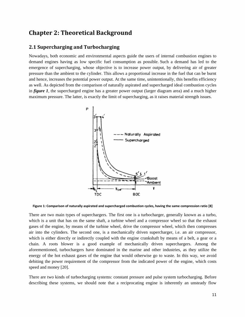
as well. As depicted from the comparison of naturally aspirated and supercharged ideal combustion cycles

in figure 1, the supercharged engine has a greater power output (larger diagram area) and a much higher

maximum pressure. The latter, is exactly the limit of supercharging, as it raises material strength issues.

Figure 1: Comparison of naturally aspirated and supercharged combustion cycles, having the same compression ratio [8]

There are two main types of superchargers. The first one is a turbocharger, generally known as a turbo,

which is a unit that has on the same shaft, a turbine wheel and a compressor wheel so that the exhaust

gases of the engine, by means of the turbine wheel, drive the compressor wheel, which then compresses

air into the cylinders. The second one, is a mechanically driven supercharger, i.e. an air compressor,

which is either directly or indirectly coupled with the engine crankshaft by means of a belt, a gear or a

chain. A roots blower is a good example of mechanically driven superchargers. Among the

aforementioned, turbochargers have dominated in the marine and other industries, as they utilize the

energy of the hot exhaust gases of the engine that would otherwise go to waste. In this way, we avoid

debiting the power requirement of the compressor from the indicated power of the engine, which costs

speed and money [20].

There are two kinds of turbocharging systems: constant pressure and pulse system turbocharging. Before

describing these systems, we should note that a reciprocating engine is inherently an unsteady flow

12

device, with each cylinder exhausting in turn at intervals during the cycle. On the contrary, compressors

and turbines operate efficiently under steady flow conditions, but can be designed to accept such an

unsteady flow. Therefore, the combination of engine and turbine is a difficult issue.

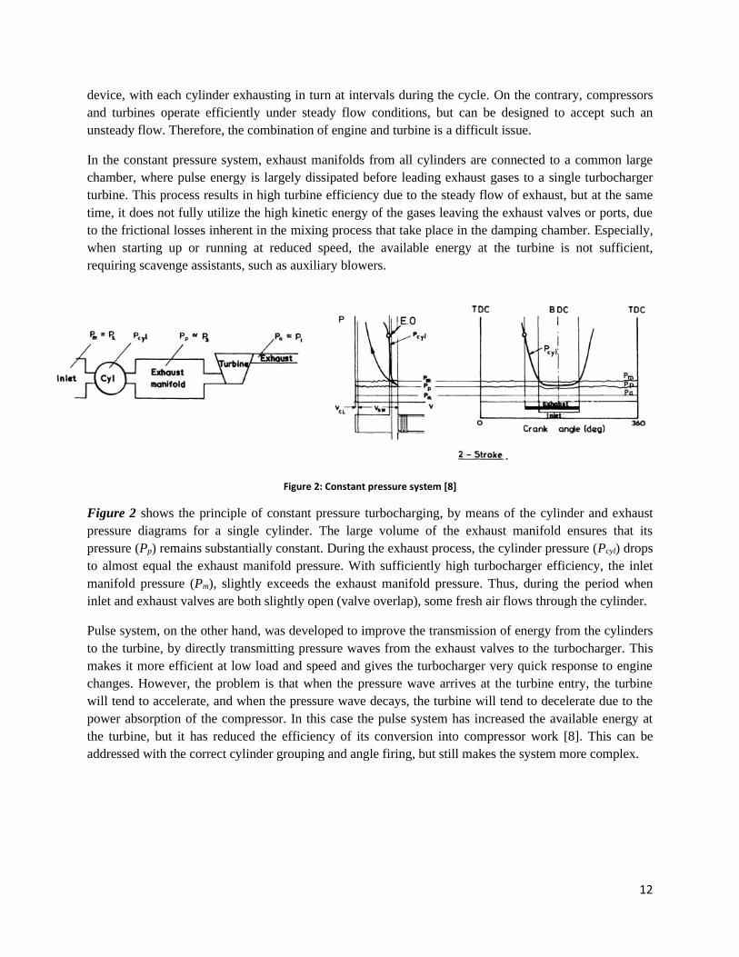
In the constant pressure system, exhaust manifolds from all cylinders are connected to a common large

chamber, where pulse energy is largely dissipated before leading exhaust gases to a single turbocharger

turbine. This process results in high turbine efficiency due to the steady flow of exhaust, but at the same

time, it does not fully utilize the high kinetic energy of the gases leaving the exhaust valves or ports, due

to the frictional losses inherent in the mixing process that take place in the damping chamber. Especially,

when starting up or running at reduced speed, the available energy at the turbine is not sufficient,

requiring scavenge assistants, such as auxiliary blowers.

Figure 2: Constant pressure system [8]

Figure 2 shows the principle of constant pressure turbocharging, by means of the cylinder and exhaust

pressure diagrams for a single cylinder. The large volume of the exhaust manifold ensures that its

pressure (Pp) remains substantially constant. During the exhaust process, the cylinder pressure (Pcyl) drops

to almost equal the exhaust manifold pressure. With sufficiently high turbocharger efficiency, the inlet

manifold pressure (Pm), slightly exceeds the exhaust manifold pressure. Thus, during the period when

inlet and exhaust valves are both slightly open (valve overlap), some fresh air flows through the cylinder.

Pulse system, on the other hand, was developed to improve the transmission of energy from the cylinders

to the turbine, by directly transmitting pressure waves from the exhaust valves to the turbocharger. This

makes it more efficient at low load and speed and gives the turbocharger very quick response to engine

changes. However, the problem is that when the pressure wave arrives at the turbine entry, the turbine

will tend to accelerate, and when the pressure wave decays, the turbine will tend to decelerate due to the

power absorption of the compressor. In this case the pulse system has increased the available energy at

the turbine, but it has reduced the efficiency of its conversion into compressor work [8]. This can be

addressed with the correct cylinder grouping and angle firing, but still makes the system more complex.

13

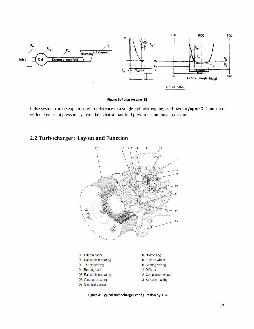
Figure 3: Pulse system [8]

Pulse system can be explained with reference to a single-cylinder engine, as shown in figure 3. Compared

with the constant pressure system, the exhaust manifold pressure is no longer constant.

2.2 Turbocharger: Layout and Function

Figure 4: Typical turbocharger configuration by ABB

14

The turbocharger is a turbomachine that consists of a turbine and a compressor, both mounted onto a

common shaft. The exhaust gases from the diesel engine flow through the gas inlet casing (07) and nozzle

ring (08) to the turbine wheel and provide the rotating torque to the turbine shaft. The exhaust gases

escape to the atmosphere through an exhaust gas pipe which is connected to the gas outlet casing (06).

Usually, seal rings and heat shields are provided so that gas may not adversely affect the bearings. The

compressor wheel (12), fitted to the turbine shaft, receives the rotating torque and induces air through the

filter silencer (01). The air then passes through the diffuser (11) and leaves the turbocharger through the

air outlet casing (13) [6]. A thrust bearing (03) is provided to receive the trust force applied to the turbine

shaft. A partition wall separates the air from the gas. In addition, usually two auxiliary air blowers are

fitted to ensure sufficient cylinder scavenging at low load engine operation.

Apart from the compressor, a second piece of equipment is used to increase further air density, known as

an intercooler or Charge Air Cooler (CAC). This is a device used for cooling the air compressed by a

supercharger before it enters the engine cylinders. In other words, a decrease in air intake temperature

provides a denser intake charge to the engine and allows more air and fuel to be combusted per engine

cycle, increasing the output of the engine [20].

An issue concerning the operation of the turbochargers, especially the constant system ones, is that, under

transient loading conditions, the response of the turbocharged marine diesel engines is limited by the

turbocharger behavior. During acceleration, it takes time for pressure to be increased in the exhaust and

scavenge receiver. Furthermore, part of the turbine power is spent to accelerate the turboshaft. Thus, the

engine boost pressure will be lower than the one corresponding to steady state conditions. On the other

hand, during fast deceleration, fuel is reduced immediately, but due to the inertia of the turbocharger’s

rotating parts, the compressor pressure ratio is greater than the one corresponding to steady state

conditions. Under such conditions, the compressor operation might become unstable.

2.2.1 Compressor Performance

There two types of compressors: axial and centrifugal. This thesis focuses on centrifugal compressors, but

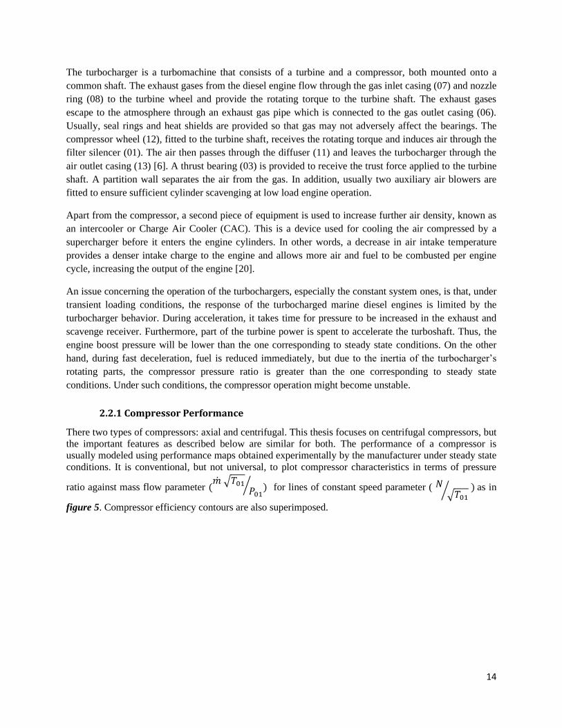
the important features as described below are similar for both. The performance of a compressor is

usually modeled using performance maps obtained experimentally by the manufacturer under steady state

conditions. It is conventional, but not universal, to plot compressor characteristics in terms of pressure

ratio against mass flow parameter (�̇� √𝑇01

𝑃01⁄ ) for lines of constant speed parameter ( 𝑁

√𝑇01⁄ ) as in

figure 5. Compressor efficiency contours are also superimposed.

15

Figure 5: Compressor characteristic [8]

There are essentially three areas on a compressor map. The central area is the stable operating zone. This

area is separated from the unstable area on its left by the surge line. Specifically, when the mass flow rate

through a compressor is reduced while maintaining a constant pressure ratio, a point arises at which local

flow reversal occurs in the boundary layers. This should result in low efficiency but not necessarily in

instability. If the flow rate is further reduced, complete reversal occurs. This will relieve the adverse

pressure gradient until a new flow regime at a lower pressure ratio is established. The flow will then build

up again to the initial condition and thus, flow instability will continue at a fixed frequency. Surge is

actually a more complex phenomenon than above described, but further explanation is out of the scope of

this thesis. It is important to point out that the compressor must not be asked to work in the area to the left

of the surge line. The area to the right of the compressor map is associated with very high gas velocity. It

is the result of choking of the limiting flow area in the machine. Extra mass flow through the compressor

can only be gained by higher speeds. This additional mass flow will certainly be limited by the ability of

the diffuser area to accept the flow. When diffuser choking occurs, compressor speed may rise

substantially with little increase in mass flow rate. The area of maximum efficiency naturally falls in the

central stable operating zone [9].

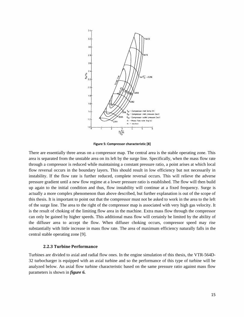
2.2.3 Turbine Performance

Turbines are divided to axial and radial flow ones. In the engine simulation of this thesis, the VTR-564D-

32 turbocharger is equipped with an axial turbine and so the performance of this type of turbine will be

analyzed below. An axial flow turbine characteristic based on the same pressure ratio against mass flow

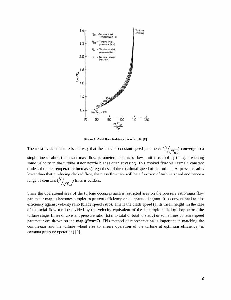
parameters is shown in figure 6.

16

Figure 6: Axial flow turbine characteristic [8]

The most evident feature is the way that the lines of constant speed parameter (𝑁√𝑇03

⁄ ) converge to a

single line of almost constant mass flow parameter. This mass flow limit is caused by the gas reaching

sonic velocity in the turbine stator nozzle blades or inlet casing. This choked flow will remain constant

(unless the inlet temperature increases) regardless of the rotational speed of the turbine. At pressure ratios

lower than that producing choked flow, the mass flow rate will be a function of turbine speed and hence a

range of constant (𝑁√𝑇03

⁄ ) lines is evident.

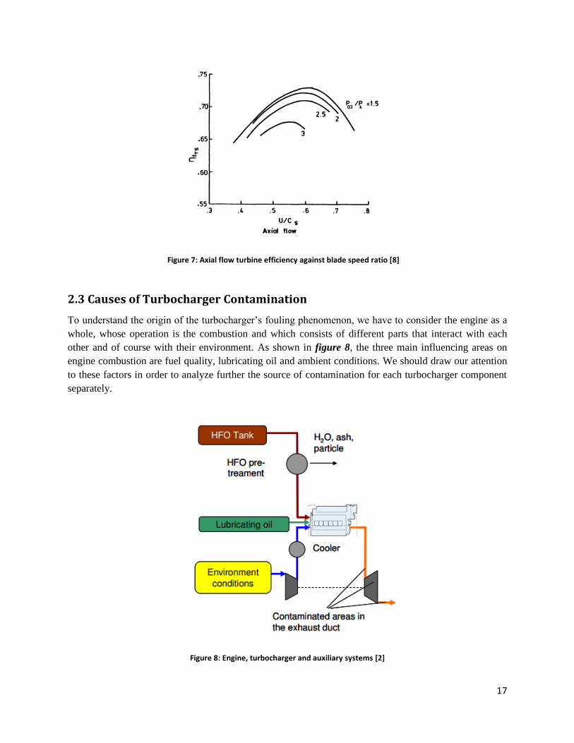
Since the operational area of the turbine occupies such a restricted area on the pressure ratio/mass flow

parameter map, it becomes simpler to present efficiency on a separate diagram. It is conventional to plot

efficiency against velocity ratio (blade speed ratio). This is the blade speed (at its mean height) in the case

of the axial flow turbine divided by the velocity equivalent of the isentropic enthalpy drop across the

turbine stage. Lines of constant pressure ratio (total to total or total to static) or sometimes constant speed

parameter are drawn on the map (figure7). This method of representation is important in matching the

compressor and the turbine wheel size to ensure operation of the turbine at optimum efficiency (at

constant pressure operation) [9].

17

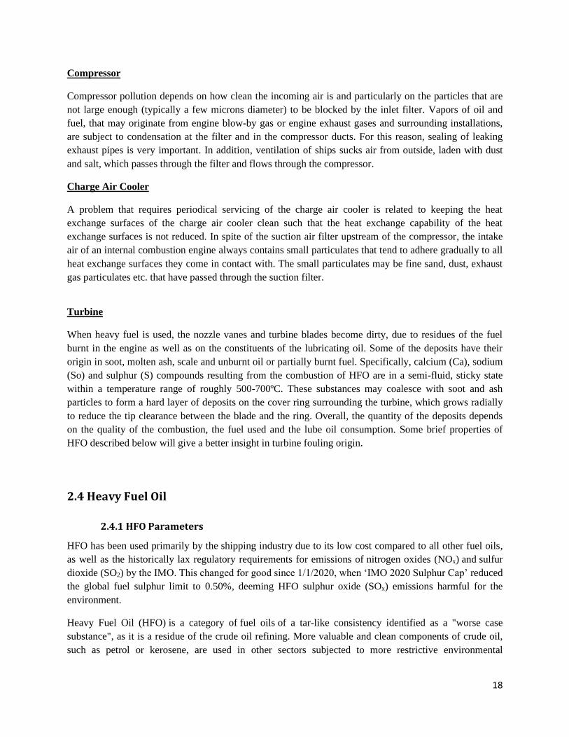
2.3 Causes of Turbocharger Contamination

To understand the origin of the turbocharger’s fouling phenomenon, we have to consider the engine as a

whole, whose operation is the combustion and which consists of different parts that interact with each

other and of course with their environment. As shown in figure 8, the three main influencing areas on

engine combustion are fuel quality, lubricating oil and ambient conditions. We should draw our attention

to these factors in order to analyze further the source of contamination for each turbocharger component

separately.

Figure 8: Engine, turbocharger and auxiliary systems [2]

Figure 7: Axial flow turbine efficiency against blade speed ratio [8]

18

Compressor

Compressor pollution depends on how clean the incoming air is and particularly on the particles that are

not large enough (typically a few microns diameter) to be blocked by the inlet filter. Vapors of oil and

fuel, that may originate from engine blow-by gas or engine exhaust gases and surrounding installations,

are subject to condensation at the filter and in the compressor ducts. For this reason, sealing of leaking

exhaust pipes is very important. In addition, ventilation of ships sucks air from outside, laden with dust

and salt, which passes through the filter and flows through the compressor.

Charge Air Cooler

A problem that requires periodical servicing of the charge air cooler is related to keeping the heat

exchange surfaces of the charge air cooler clean such that the heat exchange capability of the heat

exchange surfaces is not reduced. In spite of the suction air filter upstream of the compressor, the intake

air of an internal combustion engine always contains small particulates that tend to adhere gradually to all

heat exchange surfaces they come in contact with. The small particulates may be fine sand, dust, exhaust

gas particulates etc. that have passed through the suction filter.

Turbine

When heavy fuel is used, the nozzle vanes and turbine blades become dirty, due to residues of the fuel

burnt in the engine as well as on the constituents of the lubricating oil. Some of the deposits have their

origin in soot, molten ash, scale and unburnt oil or partially burnt fuel. Specifically, calcium (Ca), sodium

(So) and sulphur (S) compounds resulting from the combustion of HFO are in a semi-fluid, sticky state

within a temperature range of roughly 500-700ºC. These substances may coalesce with soot and ash

particles to form a hard layer of deposits on the cover ring surrounding the turbine, which grows radially

to reduce the tip clearance between the blade and the ring. Overall, the quantity of the deposits depends

on the quality of the combustion, the fuel used and the lube oil consumption. Some brief properties of

HFO described below will give a better insight in turbine fouling origin.

2.4 Heavy Fuel Oil

2.4.1 HFO Parameters

HFO has been used primarily by the shipping industry due to its low cost compared to all other fuel oils,

as well as the historically lax regulatory requirements for emissions of nitrogen oxides (NOx) and sulfur

dioxide (SO2) by the IMO. This changed for good since 1/1/2020, when ‘IMO 2020 Sulphur Cap’ reduced

the global fuel sulphur limit to 0.50%, deeming HFO sulphur oxide (SOx) emissions harmful for the

environment.

Heavy Fuel Oil (HFO) is a category of fuel oils of a tar-like consistency identified as a "worse case

substance", as it is a residue of the crude oil refining. More valuable and clean components of crude oil,

such as petrol or kerosene, are used in other sectors subjected to more restrictive environmental

19

regulations than shipping. As a result of this refining process, the largest part of any impurities contained

in the crude oil – sulphur, vanadium, nickel, water, etc. – remain in the residual oils, such as HFO.

In the MARPOL Marine Convention of 1973, heavy fuel oil is defined either by a density of greater than

900 kg/m³ at 15°C or a kinematic viscosity of more than 180 mm²/s at 50°C. Heavy fuel oils have large

percentages of heavy molecules such as long-chain hydrocarbons and aromatics with long-branched side

chains [24]. The slow-speed 2-stroke marine engines have a larger combustion time that offer the

sufficient time for these long-chain components to crack. As already mentioned, HFO contains various

metals and other contents that either come from the crude oil itself or are added at refinery process. Fuels

supplied to vessels are sent for fuel analysis to specialized laboratories to assess their main components

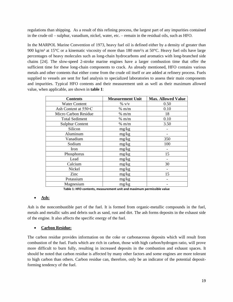
and impurities. Typical HFO contents and their measurement unit as well as their maximum allowed

value, when applicable, are shown in table 1:

Contents Measurement Unit Max. Allowed Value

Water Content % v/v 0.50

Ash Content at 550◦C % m/m 0.10

Micro Carbon Residue % m/m 18

Total Sediment % m/m 0.10

Sulphur Content % m/m 3.50

Silicon mg/kg -

Aluminum mg/kg -

Vanadium mg/kg 350

Sodium mg/kg 100

Iron mg/kg -

Phosphorus mg/kg 15

Lead mg/kg -

Calcium mg/kg 30

Nickel mg/kg -

Zinc mg/kg 15

Potassium mg/kg -

Magnesium mg/kg - Table 1: HFO contents, measurement unit and maximum permissible value

• Ash:

Ash is the noncombustible part of the fuel. It is formed from organic-metallic compounds in the fuel,

metals and metallic salts and debris such as sand, rust and dirt. The ash forms deposits in the exhaust side

of the engine. It also affects the specific energy of the fuel.

• Carbon Residue:

The carbon residue provides information on the coke or carbonaceous deposits which will result from

combustion of the fuel. Fuels which are rich in carbon, those with high carbon/hydrogen ratio, will prove

more difficult to burn fully, resulting in increased deposits in the combustion and exhaust spaces. It

should be noted that carbon residue is affected by many other factors and some engines are more tolerant

to high carbon than others. Carbon residue can, therefore, only be an indicator of the potential deposit-

forming tendency of the fuel.

20

• Sediment:

Sediment is the amount of insoluble substances in fuel. It is the rust, sand, scale and dirt which are not

part of the fuel, but can also include asphaltenic and waxy sludge, which, whilst normally dissolved or in

suspension in the fuel, can settle out and block up filters or other parts of the fuel system.

• Sulphur (S):

Sulphur is found in all crude oils and is not removed from residual fuel oil during refining, if

desulphurization doesn’t take place. Its quantity affects the exhaust emissions and acid deposition within

the cylinder of the engines.

• Silicon (Si):

Silicon is one element used as a catalyst in the catalytic conversion plant in a refinery and is always

present in conjunction with aluminum. The proportion of aluminum to silicon varies from one proprietary

catalyst to another. It can be from other contaminant sources as well.

• Aluminum (Al):

Silicon is one element used as a catalyst in the catalytic conversion plant in a refinery and is always

present in conjunction with silicon. The proportion of aluminum to silicon varies from one proprietary

catalyst to another.

• Vanadium (V):

Vanadium is a metal found in crude oil from certain geographical areas (especially western Venezuela). It

is present in the resultant fuel and in addition to its contribution to the ash level, it can, with any sodium

present, form compounds which depress the melting point of the ash in the exhaust.

• Sodium (Na):

Sodium is a metal found in crude oil. Its presence can also be the result of the use of sodium hydroxide to

remove hydrogen sulphide in the refinery process, but it is also present as salt in sea water. It can be

present in the fuel leaving the refinery or present as a contaminant from transportation.

• Iron (Fe):

Any iron found in the fuel oil comes from iron particles from pipelines and valves and from the wear of

moving metal components. It also comes from rust. Iron from engine wear can be found in any waste

automotive lubricating oil added to the fuel.

• Phosphorus (P):

Phosphorus forms part of the ‘signature’ indicating the presence of lubricating oil.

• Lead (Pb):

21

Lead can be present if waste lubricating oil from gasoline engines using leaded gasoline has been added

to the fuel.

• Calcium (Ca):

Calcium can be present in crude oil but also forms part of the ‘signature’ indicating the presence of

lubricating oil.

• Nickel (Ni):

Nickel is an element that comes from crude oil. It is tested in order to provide a ‘signature’ for an oil

sample. Suphur, vanadium and nickel content cannot be reduced by treatment, so two samples claiming to

be of the same oil, if they are the same oil, will have very similar levels of sulphur, vanadium and nickel.

• Zinc (Zn):

Zinc can be present in trace amounts in crude oil but also forms part of the ‘signature’ indicating the

presence of lubricating oil.

• Potassium (K):

Potassium can be present if potassium hydroxide has been used in the refinery process to remove

hydrogen sulphide.

• Magnesium (Mg):

Magnesium is from salts in sea water. The presence of magnesium will allow the determination of the

proportion of sodium attributable to sea water. [10]

2.4.2 Onboard Fuel Oil Treatment

After the laboratory analysis and assuming that the fuel is deemed appropriate for combustion, the fuel

must be treated on board before use in order to remove some of the above mentioned solid as well as

liquid contaminants. The solid contaminants in the fuel are mainly rust, sand, dust and refinery catalysts.

Liquid contaminants are mainly fresh or sea water. The settling tank is the first step in the fuel treatment

process. Water and sediments can be separated by gravity and drained off at the bottom of the tank.

Effective cleaning of residual fuels can only be ensured by centrifuges: a clarifier to separate particles

and/ or a purifier to separate water. The third step to remove any solid particles not separated by

centrifuging, is fine filters, usually called hot filters, which are placed directly after the centrifuge, or in

the supply line before the engine. While in purifiers separation method uses the difference in component’s

density, filters separate impurities according to their size. Most common used are the backflushing filters,

which are automatically cleaned. When they start to clog up, a differential pressure sensor initiates a

backflushing routine so that the filters clean themselves [21].

22

2.5 Indicators and Results of Fouling

Turbocharger condition is critical for the performance of turbocharged diesel engines and especially large

scale 2-stroke ones. During operation of the turbocharger and combustion of HFO, a certain amount of

particles condensates and deposits on the compressor and turbine surfaces with far-reaching consequences

for the turbocharger and the engine, as already explained. Continued operation with dirty components can

lead to a significant drop in turbocharger efficiency and even surging, mechanical malfunction, vibrations

and derated engine power output or even failure. The deposited particles additionally exhibit undesired

properties like corrosion and sticking effects, which depends largely on the particles’ composition. Not all

turbocharger components are affected in the same way and to the same extend by fouling, so below we

will give a brief description of how contamination affects each of the main ones.

Air filter

Air filter and inlet valves are the first obstacles when air passes through to reach the compressor. As the

filter gets contaminated, an active sectional area of the air through the filter gets smaller which leads to

the reduction of the air pressure value before the compressor. With the maintained compression degree πs

unchanged, the value of the air pressure behind the compressor p02 is reduced. The increase of the

negative pressure at the compressor inlet, in order to keep the set value of the rpm of the engine, causes an

increase of a fuel dose (resulting from speed regulator activation). Because the air mass flux through the

engine is smaller, the increased fuel dose causes an increase in the temperature of the outlet exhaust gases

and an increase of the specific fuel consumption be. Of course, a worst-case scenario includes the start of

surging, which is highly undesirable.

Compressor

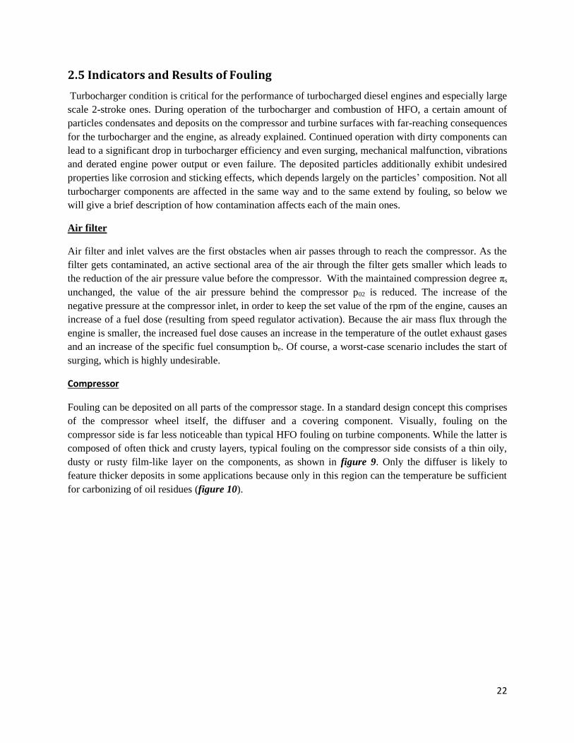
Fouling can be deposited on all parts of the compressor stage. In a standard design concept this comprises

of the compressor wheel itself, the diffuser and a covering component. Visually, fouling on the

compressor side is far less noticeable than typical HFO fouling on turbine components. While the latter is

composed of often thick and crusty layers, typical fouling on the compressor side consists of a thin oily,

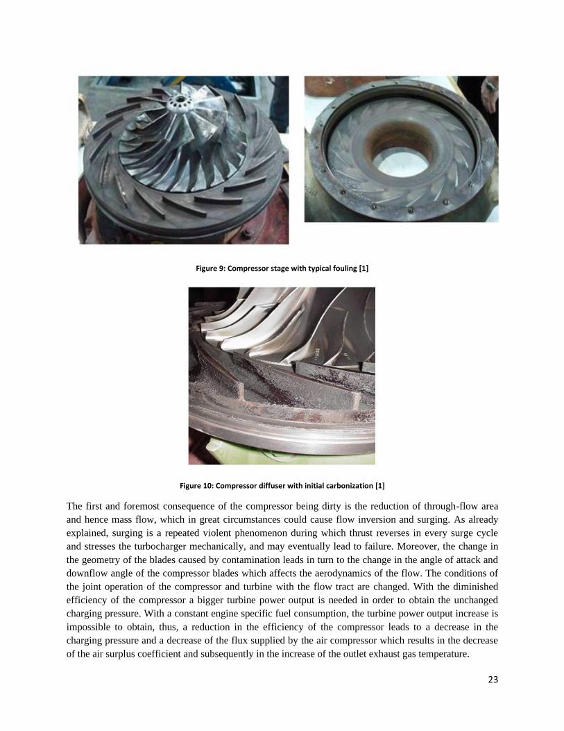
dusty or rusty film-like layer on the components, as shown in figure 9. Only the diffuser is likely to

feature thicker deposits in some applications because only in this region can the temperature be sufficient

for carbonizing of oil residues (figure 10).

23

Figure 9: Compressor stage with typical fouling [1]

Figure 10: Compressor diffuser with initial carbonization [1]

The first and foremost consequence of the compressor being dirty is the reduction of through-flow area

and hence mass flow, which in great circumstances could cause flow inversion and surging. As already

explained, surging is a repeated violent phenomenon during which thrust reverses in every surge cycle

and stresses the turbocharger mechanically, and may eventually lead to failure. Moreover, the change in

the geometry of the blades caused by contamination leads in turn to the change in the angle of attack and

downflow angle of the compressor blades which affects the aerodynamics of the flow. The conditions of

the joint operation of the compressor and turbine with the flow tract are changed. With the diminished

efficiency of the compressor a bigger turbine power output is needed in order to obtain the unchanged

charging pressure. With a constant engine specific fuel consumption, the turbine power output increase is

impossible to obtain, thus, a reduction in the efficiency of the compressor leads to a decrease in the

charging pressure and a decrease of the flux supplied by the air compressor which results in the decrease

of the air surplus coefficient and subsequently in the increase of the outlet exhaust gas temperature.

24

Besides affecting the efficiency, the layer of soot on the compressor contains sulphur, which has a

corrosive effect on the aluminum alloy and can lead to a considerable reduction in the fatigue resistance

of the inducer and compressor wheels.

Air cooler

When it comes to contamination of the air cooler, pressure loss increases and charge air becomes hotter,

air density becomes lower and less air is induced in the cylinders. Fouled air cooler and water mist

catcher are considered one the most common reasons for turbocharger’s surging.

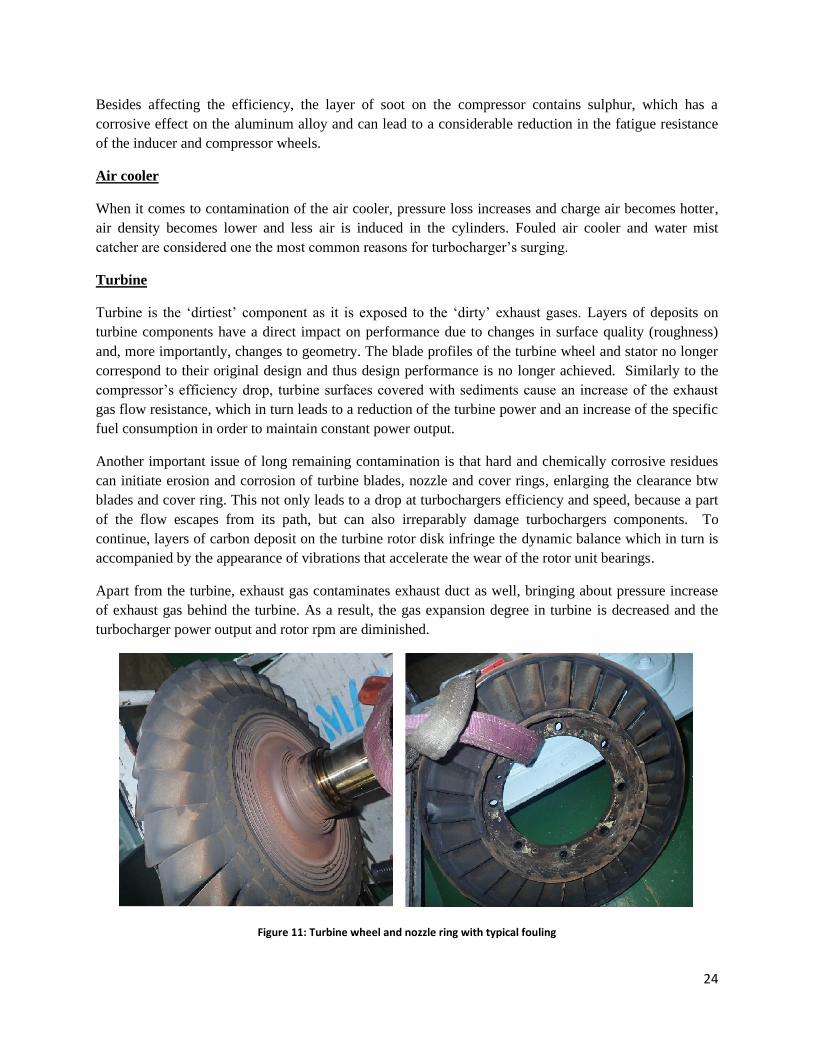
Turbine

Turbine is the ‘dirtiest’ component as it is exposed to the ‘dirty’ exhaust gases. Layers of deposits on

turbine components have a direct impact on performance due to changes in surface quality (roughness)

and, more importantly, changes to geometry. The blade profiles of the turbine wheel and stator no longer

correspond to their original design and thus design performance is no longer achieved. Similarly to the

compressor’s efficiency drop, turbine surfaces covered with sediments cause an increase of the exhaust

gas flow resistance, which in turn leads to a reduction of the turbine power and an increase of the specific

fuel consumption in order to maintain constant power output.

Another important issue of long remaining contamination is that hard and chemically corrosive residues

can initiate erosion and corrosion of turbine blades, nozzle and cover rings, enlarging the clearance btw

blades and cover ring. This not only leads to a drop at turbochargers efficiency and speed, because a part

of the flow escapes from its path, but can also irreparably damage turbochargers components. To

continue, layers of carbon deposit on the turbine rotor disk infringe the dynamic balance which in turn is

accompanied by the appearance of vibrations that accelerate the wear of the rotor unit bearings.

Apart from the turbine, exhaust gas contaminates exhaust duct as well, bringing about pressure increase

of exhaust gas behind the turbine. As a result, the gas expansion degree in turbine is decreased and the

turbocharger power output and rotor rpm are diminished.

Figure 11: Turbine wheel and nozzle ring with typical fouling

25

2.6 Importance of Cleanness

The integration of the available cleaning methods into the turbocharger design and development process

aims to narrow the gap between the performance potential of turbocharger technology and the

performance effectively available over standard service intervals. As described above, engine operation

can be disturbed considerably by the build-up of contamination, causing from substantial flow

disturbances to mechanical malfunction and wear up to derated engine power output.

From a broader perspective, the importance of the right maintenance of mechanical parts is emphasized

now more than ever with the establishment of Planned Maintenance System (PMS) by almost all vessel

operators. They have realized that proper maintenance is the only way, not only to avoid the additional

costs of new spare parts and labor hours, but also to narrow down the possibility of the vessel

experiencing unwanted breakdowns and delays, with major legal and economic impacts.

2.7 Cleaning Procedures and Intervals

The adverse and dirty working environment as described above created the need to develop some

cleaning procedures that would, if not eliminate, at least reduce contamination and thus, maintain the

engine’s good working condition. The obvious cleaning method is the one done during overhauls, where

the turbocharger among other engine components is completely dismantled and thoroughly cleaned part

by part. During dismantling, turbocharger sometimes is professionally rebalanced on a proper balancing

machine to be sure that it runs smoothly and that bearing loads are minimized. Dismantling intervals,

which is recommended between 8000 and 16000 hours of operation, can be delayed by periodic cleaning.

The prevailing cleaning methods for the turbocharger while in operation are wet and dry cleaning.

Wet cleaning can be applied in both turbine and compressor and is performed by using only fresh water.

Water injection method is based on the mechanical effect of impinging droplets of water and, since the

liquid does not act as a solvent, there is no need to add chemicals. The use of saltwater is not allowed, as

it is highly corrosive for the aluminum compressor wheel and other parts of the engine [3].

On the other hand, dry cleaning, which is applicable only to the turbine, uses commercial granules, such

as nutshells, activated charcoal (soft), with particle size 1.0mm (max 1.5mm). The layers of deposits on

components’ surfaces are removed by the kinetic energy of the granules, causing them to act as an

abrasive.

2.7.1 Compressor’s Cleaning Procedure

Compressor’s wet cleaning is performed during operation at full load of the engine (at the highest

possible speed), so that water droplets acquire the maximum kinetic energy. The complete content of the

water vessel should be injected within 4 to 10 seconds. Successful cleaning is indicated by a change in the

charge air or scavenging pressure, and in most cases by a drop in the exhaust gas temperature. If cleaning

has not produced the desired results, it can be repeated after 10 minutes. Generally, wet cleaning of the

compressor needs to be done every 1 to 3 days [3].

26

2.7.2 Turbine’s Cleaning Procedure

Wet cleaning of the turbine’s side is applied in both 2-stoke and 4-stroke engines and the cleaning

mechanism is described as follows: The washing water droplets bounce against the nozzle ring and

turbine wheel, where they wear off deposits by mechanical cleaning. At the same time, not only does the

water act as a dissolvent for some chemical residues, but it also evaporates on metal’s surface, causing

drop in surface temperature. The contraction of turbine blade material resulting from this cooling makes

the deposits to crack off. The quantity of injected water is precisely specified by the manufacturer and

depends on the exhaust gas temperature, water pressure, size of turbocharger and number of gas inlets.

Wet cleaning must take place approximately every 250 operating hours or 1 to 20 days.

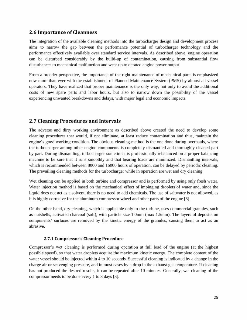
It is of great importance that this kind of

washing is done during a heavily reduced

engine load to avoid overload of the

turbine blades. Otherwise, the contact of

water droplets with the high temperature

turbine wheel would cause thermal shock,

during which surface layers contract

against the inner layers, leading to the

development of tensile stress and the

propagation of cracks. For this reason, the

exhaust gas temperature should not exceed

430 ·C. At the same time, boost pressure

must be above 0.3 bar to prevent water

from entering the turbine end oil chamber.

Figure 12 suggests waiting for a certain

length of time before and after washing and while being in reduced load, in order to give the material time

to adapt to the exhaust gas temperature, and to eliminate the possibility of crack formation and

propagation [3].

Dry cleaning of the turbine is applicable only in 2-stroke engines and seems to be the most commonly

used in the shipping industry. Its convenience of performing the cleaning operation at normal load of

engine, counterbalances the drawback of removing only thin layers of deposits and thus needing shorter

cleaning intervals compared to wet cleaning. Exhaust gas temperature should not exceed 580 ·C , boost

pressure has to be above 0.5 bar and the quantity needed varies from 0.2l to 3l, according to

manufacturer’s instructions and depending on the size of the turbocharger. Dry cleaning intervals vary

from 24 to 50 hours of operation (1 to 2 days).

Worries about erosion of turbine parts are eliminated by manufacturers, provided that the cleaning

instructions are followed carefully. Assuming that turbine cleaning is carried out 250 times per year for

about 20 seconds, the turbine will be subjected to washing impact for less than 2 hours. This is a minor

percentage if we assume 6,000 hours of operation for a typical turbocharger. Of course, erosion takes

place due to particles in the exhaust gas, but this is out of the scope of this research.

Figure 12: Procedure for turbine washing [3]

27

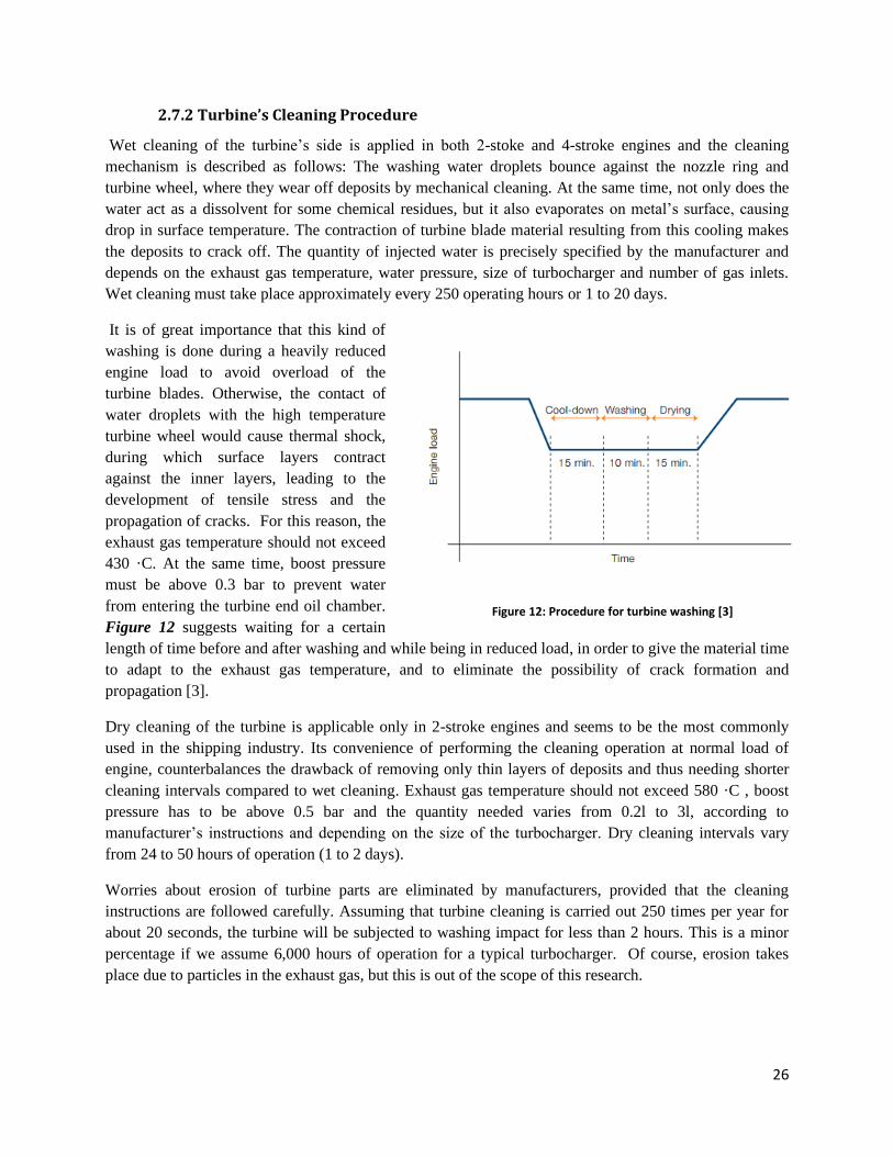
2.7.3 Mechanically cleaning during overhauls

Disassembly and assembly of the turbocharger for cleaning and servicing purpose is analytically

described in the manufacturer’s manual. Generally, it is important to keep in mind that turbocharger

components are sensitive to mechanical damage, as the use of needle guns or other impact tools, for

example, damages the components. Depending on the specification, nozzle rings have protective coatings,

which can also be damaged. Therefore, only the use of soft tools such as scouring cloths, brushes or wire

brushes is permitted. In the event of heavy contamination, the cleaning methods, such as soaking, can be

repeated until a satisfactory result has been achieved [6].

Figure 13: Compressor, Turbine wheel and their shaft taken out for overhauling

2.7.4 Cleaning Intervals

The above-mentioned cleaning intervals are given by manufacturers on an indicative basis and are

neither precise nor absolutely correct. As already mentioned, fouling depends on fuel properties as well as

on combustion quality and consequently, the following cleaning plan must be planned and executed

according to the actual need of each turbocharger and engine, neither too often nor too seldom. If washing

is carried out too often, the cleaning results will be good, but the thermal cycles increase, which causes

material stress and may impact component durability, especially if the washing temperature is too high.

Thermal stress not only can cause cracking but the more thermal cycles, the faster the cracks develop and

propagate, and the smaller the component’s life will be. If, instead, the intervals between washings are too

long, more dirt will build up, causing a drop in turbocharger efficiency, blockage of air paths and an

increase in the exhaust gas temperature [3]. Heavily contaminated turbines, which were not cleaned

periodically from the beginning or after an overhaul, cannot be cleaned by periodic cleaning methods but

only by mechanical cleaning. Generally, the best approach to this problem is the iterative one, where

engine operators are constantly monitoring exhaust gas temperature and pressure as main indicators of

turbochargers condition.

28

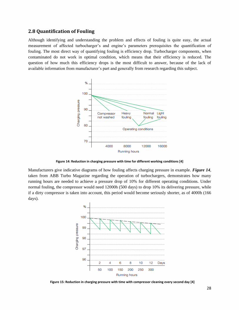
2.8 Quantification of Fouling

Although identifying and understanding the problem and effects of fouling is quite easy, the actual

measurement of affected turbocharger’s and engine’s parameters prerequisites the quantification of

fouling. The most direct way of quantifying fouling is efficiency drop. Turbocharger components, when

contaminated do not work in optimal condition, which means that their efficiency is reduced. The

question of how much this efficiency drops is the most difficult to answer, because of the lack of

available information from manufacturer’s part and generally from research regarding this subject.

Figure 14: Reduction in charging pressure with time for different working conditions [4]

Manufacturers give indicative diagrams of how fouling affects charging pressure in example. Figure 14,

taken from ABB Turbo Magazine regarding the operation of turbochargers, demonstrates how many

running hours are needed to achieve a pressure drop of 10% for different operating conditions. Under

normal fouling, the compressor would need 12000h (500 days) to drop 10% its delivering pressure, while

if a dirty compressor is taken into account, this period would become seriously shorter, as of 4000h (166

days).

Figure 15: Reduction in charging pressure with time with compressor cleaning every second day [4]

29

Another useful diagram (figure 15) demonstrates a 1% pressure drop between washing with a 2 days

interval. An interesting remark is that pressure descends gradually over time, albeit periodic cleaning.

This is exactly the reason why dismantling and mechanical cleaning is necessary to fully restore

turbocharger’s condition.

The above diagrams are useful but only on an indicative basis, as they give information about one result

of fouling, charging pressure drop, and not the ‘root’ of these results, meaning efficiency decline. A major

source of our research was the Paper No.170, ‘Turbocharger Performance Stability under HFO

Conditions’ [1], which quantifies the distinct efficiency gain for the different turbine components due to

cleaning after severe HFO operation. During this research, turbochargers operating under harsh HFO

conditions were returned from the field and investigated on a burner test rig. The turbochargers were

cleaned step by step and worn parts exchanged step by step. After each step the overall change of turbine

efficiency was measured [1]. In this way, the influence of fouling and wear is now known in more detail.

Collectively, an average efficiency drop on the turbine side was detected in the range of up to 2 to 3 % in

very severe cases. This correlated well with the phenomena measured and observed in the field.

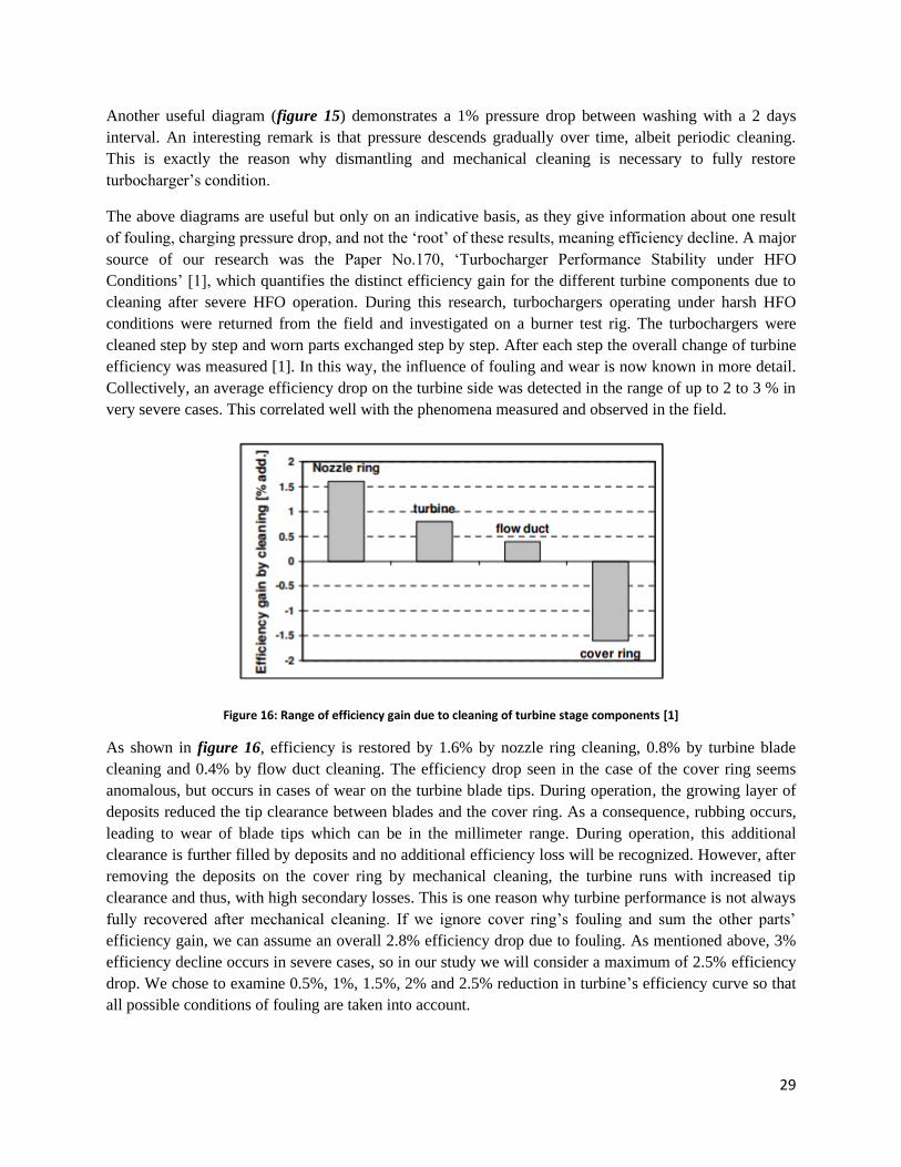
Figure 16: Range of efficiency gain due to cleaning of turbine stage components [1]

As shown in figure 16, efficiency is restored by 1.6% by nozzle ring cleaning, 0.8% by turbine blade

cleaning and 0.4% by flow duct cleaning. The efficiency drop seen in the case of the cover ring seems

anomalous, but occurs in cases of wear on the turbine blade tips. During operation, the growing layer of

deposits reduced the tip clearance between blades and the cover ring. As a consequence, rubbing occurs,

leading to wear of blade tips which can be in the millimeter range. During operation, this additional

clearance is further filled by deposits and no additional efficiency loss will be recognized. However, after

removing the deposits on the cover ring by mechanical cleaning, the turbine runs with increased tip

clearance and thus, with high secondary losses. This is one reason why turbine performance is not always

fully recovered after mechanical cleaning. If we ignore cover ring’s fouling and sum the other parts’

efficiency gain, we can assume an overall 2.8% efficiency drop due to fouling. As mentioned above, 3%

efficiency decline occurs in severe cases, so in our study we will consider a maximum of 2.5% efficiency

drop. We chose to examine 0.5%, 1%, 1.5%, 2% and 2.5% reduction in turbine’s efficiency curve so that

all possible conditions of fouling are taken into account.

30

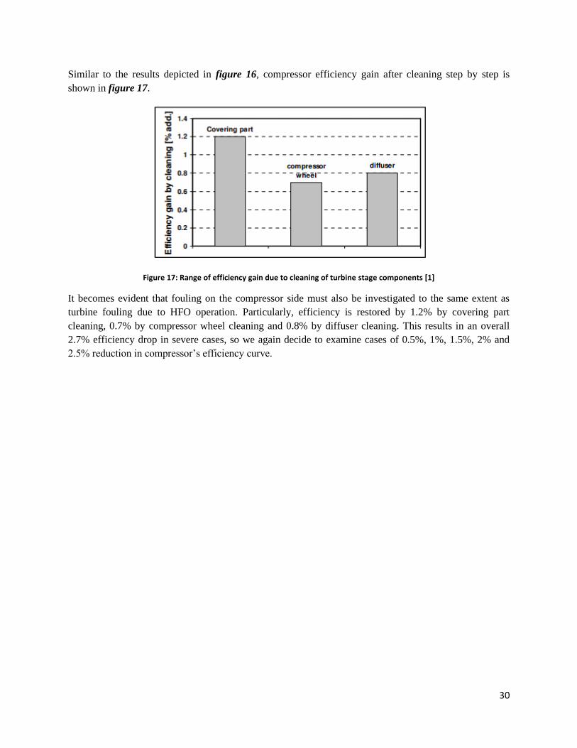
Similar to the results depicted in figure 16, compressor efficiency gain after cleaning step by step is

shown in figure 17.

Figure 17: Range of efficiency gain due to cleaning of turbine stage components [1]

It becomes evident that fouling on the compressor side must also be investigated to the same extent as

turbine fouling due to HFO operation. Particularly, efficiency is restored by 1.2% by covering part

cleaning, 0.7% by compressor wheel cleaning and 0.8% by diffuser cleaning. This results in an overall

2.7% efficiency drop in severe cases, so we again decide to examine cases of 0.5%, 1%, 1.5%, 2% and

2.5% reduction in compressor’s efficiency curve.

31

Chapter 3: Engine Model

Simulation is an important feature in engineering systems or any system that involves many processes and

is defined as an approximate imitation of the operation of a process or system. In case of internal

combustion engines, an engine model is designed in order to simulate the different processes that take

place inside a real engine, through various mathematical models and equations. A well- designed engine

model is valuable for the scientific and commercial community, as it can predict the engine’s performance

without the need of costly and time-consuming engine testing. Deep understanding of numerous engine

variables and the effect of each of them separately, and in combination as well as optimization of an

engine design to suit a particular application via parametric studies, are only a few of the capabilities of

engine simulations.

A mathematical engine simulation model is either fluid-dynamics-based or thermodynamics-based. In

fluid-dynamics-based or multidimensional models, both spatial coordinates and time are necessary in

order to accurately describe the system, thus providing us with detailed information about the spatial

properties of the fluid. However, the equations applied are partial differential equations, whose solution

requires a lot of computational data and time. On the other hand, thermodynamic-based models or zero-

dimensional models are based on the thermodynamic analysis of the cylinder contents and the only

parameter required to describe the system is time, resulting in the use of ordinary differential equations.

3.1 MOTHER Simulation Program

In the present study, the model of the engine was developed in the in-house engine simulation tool MOtor

THERmodynamics (MOTHER). MOTHER is a comprehensive thermodynamic engine performance

prediction code which falls under the category of zero-dimensional or control volume simulation models.

It considers the engine as a sequence of interconnected volumes via valves or ports, assuming spatial

uniformity of fluid properties and constant rate of change of parameters in each control volume at any

computational time step [5]. The MOTHER engine simulation code has been under development for

several years in the Laboratory of Marine Engineering and is capable of predicting the engine and

turbocharger performance under both steady-state and transient conditions.

The four governing equations that are applied in any control volume are presented below:

(3.1) �̇� = 𝑓 (�̇�, �̇�, �̇�, �̇�, �̇�)

(3.2) �̇� = 𝑓 (𝑃, 𝑇, 𝑔, 𝑅, 𝛢𝑓𝑙𝑜𝑤 , 𝐶𝑑)

(3.3) �̇� = ∑ 𝑚𝑗̇

(3.4) 𝑃 = 𝑓 (𝑚, 𝑅, 𝑇, 𝑉)

Equation (3.1) describes the non-steady flow of energy inside the control volume, expressed as the rate of

change of temperature 𝑇 ̇̇ , in terms of other parameters. The rate of change of the internal energy �̇� and

32

enthalpy �̇� of the working fluid is obtained by reference to thermodynamic property data for air/fuel

mixtures. The rate of change of equivalence ratio �̇�, is obtained by summing the air and fuel exchanges.

The rate of change of heat �̇� depends on the heat released by combustion and the heat lost due to heat

transfer. The rate of change of work �̇�, depends on the rate of change of the control volume based on the

engine geometry, as well as the instantaneous pressure [5].

Equation (3.2) gives the mass flow between interconnected volumes, which depends on the instantaneous

pressure 𝑃, temperature 𝑇, mixture properties in each volume, geometry dependent flow area 𝐴𝑓𝑙𝑜𝑤 and

discharge coefficient 𝐶𝑑 of the restrictions between the volumes (valves, ports etc.). For each control

volume and after each computational step, the Law of Conservation of Mass is applied, as described in

equation (3.3).

Finally, the equation of state (3.4) is used to determine the instantaneous pressure 𝑃, based on the actual

volume 𝑉, mass 𝑚, temperature 𝑇 and fluid properties.

The resulting set of coupled differential equations is solved numerically for all the control volumes of the

system, with a typical resolution of one-degree crank angle or smaller.

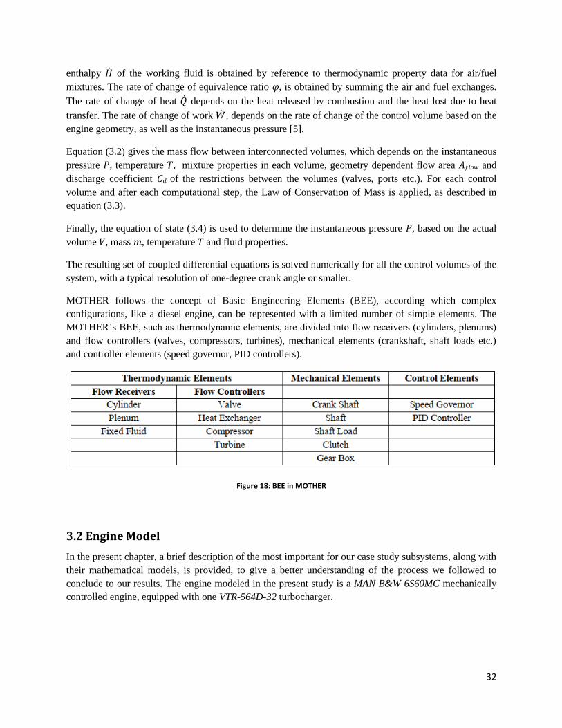
MOTHER follows the concept of Basic Engineering Elements (BEE), according which complex

configurations, like a diesel engine, can be represented with a limited number of simple elements. The

MOTHER’s BEE, such as thermodynamic elements, are divided into flow receivers (cylinders, plenums)

and flow controllers (valves, compressors, turbines), mechanical elements (crankshaft, shaft loads etc.)

and controller elements (speed governor, PID controllers).

Figure 18: BEE in MOTHER

3.2 Engine Model

In the present chapter, a brief description of the most important for our case study subsystems, along with

their mathematical models, is provided, to give a better understanding of the process we followed to

conclude to our results. The engine modeled in the present study is a MAN B&W 6S60MC mechanically

controlled engine, equipped with one VTR-564D-32 turbocharger.

33

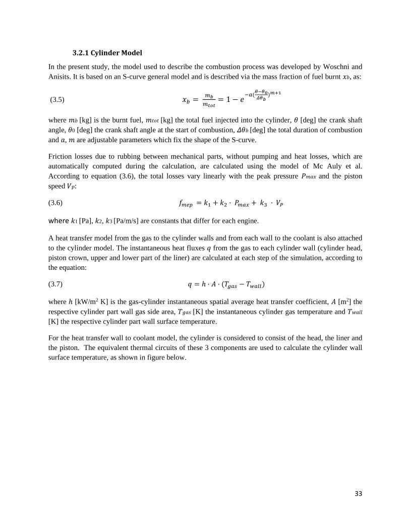
3.2.1 Cylinder Model

In the present study, the model used to describe the combustion process was developed by Woschni and

Anisits. It is based on an S-curve general model and is described via the mass fraction of fuel burnt 𝑥𝑏, as:

(3.5) 𝑥𝑏 = 𝑚𝑏

𝑚𝑡𝑜𝑡= 1 − 𝑒

−𝑎(𝜃−𝜃0𝛥𝜃𝑏

)𝑚+1

where 𝑚𝑏 [kg] is the burnt fuel, 𝑚𝑡𝑜𝑡 [kg] the total fuel injected into the cylinder, 𝜃 [deg] the crank shaft

angle, 𝜃0 [deg] the crank shaft angle at the start of combustion, 𝛥𝜃𝑏 [deg] the total duration of combustion

and 𝑎, 𝑚 are adjustable parameters which fix the shape of the S-curve.

Friction losses due to rubbing between mechanical parts, without pumping and heat losses, which are

automatically computed during the calculation, are calculated using the model of Mc Auly et al.

According to equation (3.6), the total losses vary linearly with the peak pressure 𝑃𝑚𝑎𝑥 and the piston

speed 𝑉𝑝:

(3.6) 𝑓𝑚𝑒𝑝 = 𝑘1 + 𝑘2 · 𝑃𝑚𝑎𝑥 + 𝑘3 · 𝑉𝑃

where 𝑘1 [Pa], 𝑘2, 𝑘3 [Pa/m/s] are constants that differ for each engine.

A heat transfer model from the gas to the cylinder walls and from each wall to the coolant is also attached

to the cylinder model. The instantaneous heat fluxes 𝑞 from the gas to each cylinder wall (cylinder head,

piston crown, upper and lower part of the liner) are calculated at each step of the simulation, according to

the equation:

(3.7) 𝑞 = ℎ · 𝐴 · (𝑇𝑔𝑎𝑠 − 𝑇𝑤𝑎𝑙𝑙)

where ℎ [kW/m2 K] is the gas-cylinder instantaneous spatial average heat transfer coefficient, 𝐴 [m2] the

respective cylinder part wall gas side area, 𝑇𝑔𝑎𝑠 [K] the instantaneous cylinder gas temperature and 𝑇𝑤𝑎𝑙𝑙

[K] the respective cylinder part wall surface temperature.

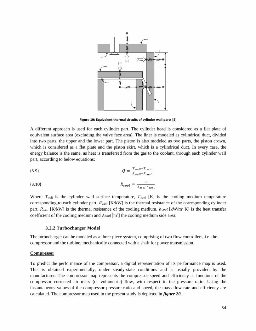
For the heat transfer wall to coolant model, the cylinder is considered to consist of the head, the liner and

the piston. The equivalent thermal circuits of these 3 components are used to calculate the cylinder wall

surface temperature, as shown in figure below.

34

Figure 19: Equivalent thermal circuits of cylinder wall parts [5]

A different approach is used for each cylinder part. The cylinder head is considered as a flat plate of

equivalent surface area (excluding the valve face area). The liner is modeled as cylindrical duct, divided

into two parts, the upper and the lower part. The piston is also modeled as two parts, the piston crown,

which is considered as a flat plate and the piston skirt, which is a cylindrical duct. In every case, the

energy balance is the same, as heat is transferred from the gas to the coolant, through each cylinder wall

part, according to below equations:

(3.9) 𝑄 = 𝑇𝑤𝑎𝑙𝑙−𝑇𝑐𝑜𝑜𝑙

𝑅𝑤𝑎𝑙𝑙−𝑅𝑐𝑜𝑜𝑙

(3.10) 𝑅𝑐𝑜𝑜𝑙 = 1

ℎ𝑐𝑜𝑜𝑙·𝐴𝑐𝑜𝑜𝑙

Where Twall is the cylinder wall surface temperature, 𝑇𝑐𝑜𝑜𝑙 [K] is the cooling medium temperature

corresponding to each cylinder part, 𝑅𝑤𝑎𝑙𝑙 [K/kW] is the thermal resistance of the corresponding cylinder

part, 𝑅𝑐𝑜𝑜𝑙 [K/kW] is the thermal resistance of the cooling medium, ℎ𝑐𝑜𝑜𝑙 [kW/m2 K] is the heat transfer

coefficient of the cooling medium and 𝐴𝑐𝑜𝑜𝑙 [m2] the cooling medium side area.

3.2.2 Turbocharger Model

The turbocharger can be modeled as a three-piece system, comprising of two flow controllers, i.e. the

compressor and the turbine, mechanically connected with a shaft for power transmission.

Compressor

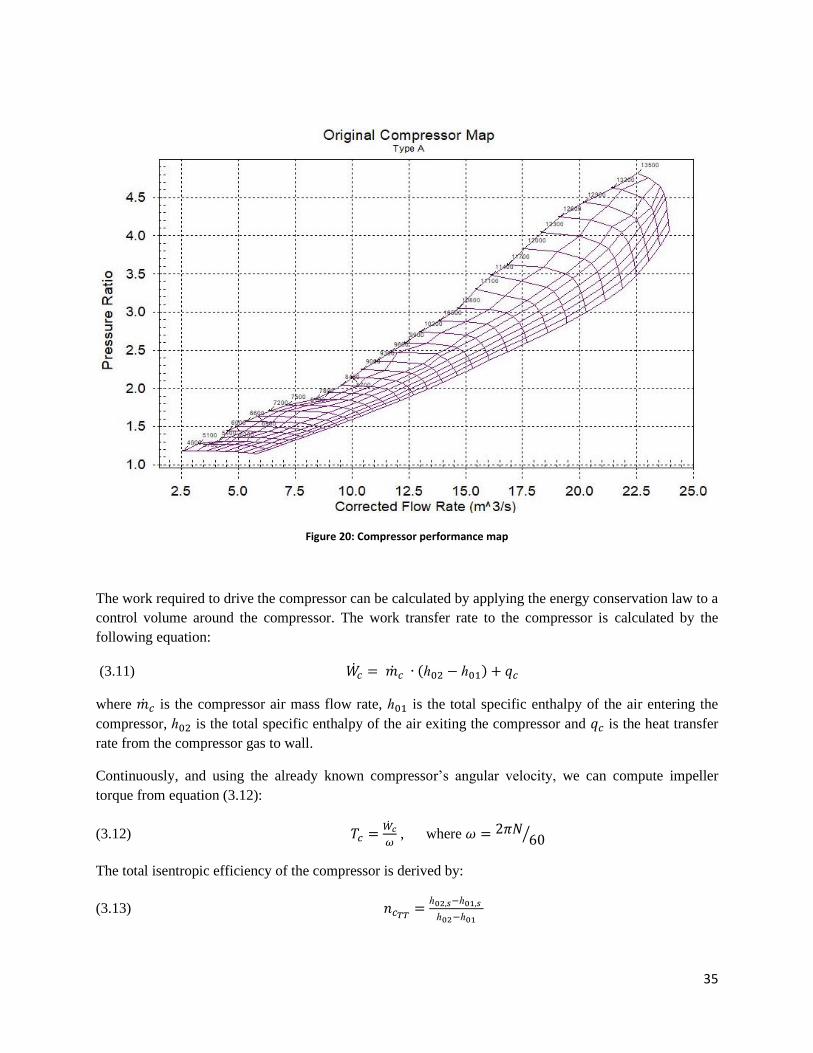
To predict the performance of the compressor, a digital representation of its performance map is used.

This is obtained experimentally, under steady-state conditions and is usually provided by the

manufacturer. The compressor map represents the compressor speed and efficiency as functions of the

compressor corrected air mass (or volumetric) flow, with respect to the pressure ratio. Using the

instantaneous values of the compressor pressure ratio and speed, the mass flow rate and efficiency are

calculated. The compressor map used in the present study is depicted in figure 20.

35

Figure 20: Compressor performance map

The work required to drive the compressor can be calculated by applying the energy conservation law to a

control volume around the compressor. The work transfer rate to the compressor is calculated by the

following equation:

(3.11) �̇�𝑐 = �̇�𝑐 ∙ (ℎ02 − ℎ01) + 𝑞𝑐

where �̇�𝑐 is the compressor air mass flow rate, ℎ01 is the total specific enthalpy of the air entering the

compressor, ℎ02 is the total specific enthalpy of the air exiting the compressor and 𝑞𝑐 is the heat transfer

rate from the compressor gas to wall.

Continuously, and using the already known compressor’s angular velocity, we can compute impeller

torque from equation (3.12):

(3.12) 𝑇𝑐 =�̇�𝑐

𝜔 , where 𝜔 = 2𝜋𝑁

60⁄

The total isentropic efficiency of the compressor is derived by:

(3.13) 𝑛𝑐𝑇𝑇=

ℎ02,𝑠−ℎ01,𝑠

ℎ02−ℎ01

36

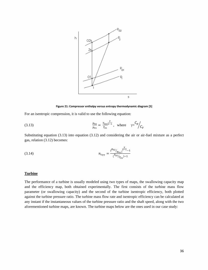
Figure 21: Compressor enthalpy versus entropy thermodynamic diagram [5]

For an isentropic compression, it is valid to use the following equation:

(3.13) 𝑝02

𝑝01=

𝑇02𝑠

𝑇01

𝛾

𝛾−1 , where γ=𝐶𝑝

𝐶𝑉⁄

Substituting equation (3.13) into equation (3.12) and considering the air or air-fuel mixture as a perfect

gas, relation (3.12) becomes:

(3.14) 𝑛𝑐𝑇𝑇=

(𝑝02

𝑝01)⁄

𝛾𝛾−1−1

(𝑇02

𝑇01⁄ )−1

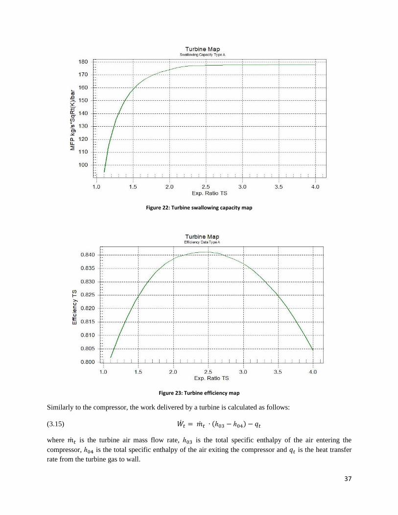
Turbine

The performance of a turbine is usually modeled using two types of maps, the swallowing capacity map

and the efficiency map, both obtained experimentally. The first consists of the turbine mass flow

parameter (or swallowing capacity) and the second of the turbine isentropic efficiency, both plotted

against the turbine pressure ratio. The turbine mass flow rate and isentropic efficiency can be calculated at

any instant if the instantaneous values of the turbine pressure ratio and the shaft speed, along with the two

aforementioned turbine maps, are known. The turbine maps below are the ones used in our case study:

37

Figure 22: Turbine swallowing capacity map

Figure 23: Turbine efficiency map

Similarly to the compressor, the work delivered by a turbine is calculated as follows:

(3.15) �̇�𝑡 = �̇�𝑡 ∙ (ℎ03 − ℎ04) − 𝑞𝑡

where �̇�𝑡 is the turbine air mass flow rate, ℎ03 is the total specific enthalpy of the air entering the

compressor, ℎ04 is the total specific enthalpy of the air exiting the compressor and 𝑞𝑡 is the heat transfer

rate from the turbine gas to wall.

38

Continuously, we can compute turbine wheel torque:

(3.16) 𝑇𝑡 =�̇�𝑡

𝜔 , where 𝜔 = 2𝜋𝑁

60⁄

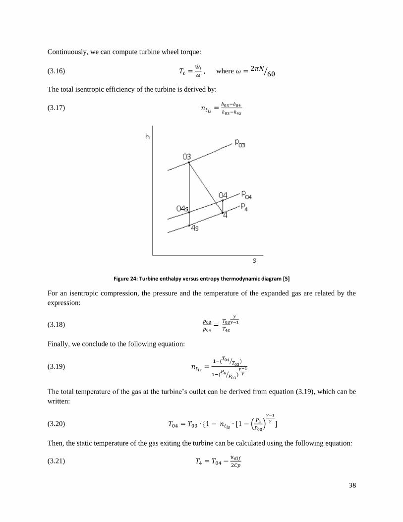
The total isentropic efficiency of the turbine is derived by:

(3.17) 𝑛𝑡𝑖𝑠=

ℎ03−ℎ04

ℎ03−ℎ4𝑧

Figure 24: Turbine enthalpy versus entropy thermodynamic diagram [5]

For an isentropic compression, the pressure and the temperature of the expanded gas are related by the

expression:

(3.18) 𝑝03

𝑝04=

𝑇03

𝑇4𝑧

𝛾

𝛾−1

Finally, we conclude to the following equation:

(3.19) 𝑛𝑡𝑖𝑠=

1−(𝑇04

𝛵03⁄ )

1−(𝑃4

𝑃03⁄ )

𝛾−1𝛾

The total temperature of the gas at the turbine’s outlet can be derived from equation (3.19), which can be

written:

(3.20) 𝑇04 = 𝛵03 ∙ {1 − 𝑛𝑡𝑖𝑠∙ [1 − (

𝑃4

𝑃03)

𝛾−1

𝛾]

Then, the static temperature of the gas exiting the turbine can be calculated using the following equation:

(3.21) 𝑇4 = 𝑇04 −𝑢𝑑𝑖𝑓

2𝐶𝑝

39

The velocity of the working medium is obtained using the mass flow equation as follows:

(3.22) 𝑢𝑑𝑖𝑓 =�̇�𝑇

𝜌∙𝛢𝑑𝑖𝑓

Finally, the static pressure of the gas exiting the turbine can be calculated using the isentropic expansion

equation for static to total ratios of pressure and temperature at the same position (see Figure 5.7):

(3.23) 𝑃4 = 𝑝04 ∙𝑇4

𝑇04

𝛾

𝛾−1

Chapter 4: Simulation Setup and Results

As already mentioned, fouling of the compressor and turbine is quantified as an efficiency drop, and

consequently as a change in the components’ maps. Having by the manufacturer the original compressor

and turbine map, we modified the efficiency curve to correspond to the 99.5%, 99%, 98.5%, 98% and

97.5% of the original value so that it represents a range of 0.5%, 1%, 1.5%,2% and 2.5% efficiency drop

due to fouling. Then, we inserted the modified compressor or turbine maps successively to MOTHER,

maintaining the other component’s map in its original form, in order to study the fouling of the

compressor or turbine separately. Steady state runs at 50%, 75% and 100% were performed to investigate

whether turbocharger fouling affects engine parameters more intensely in high or low loading operation.

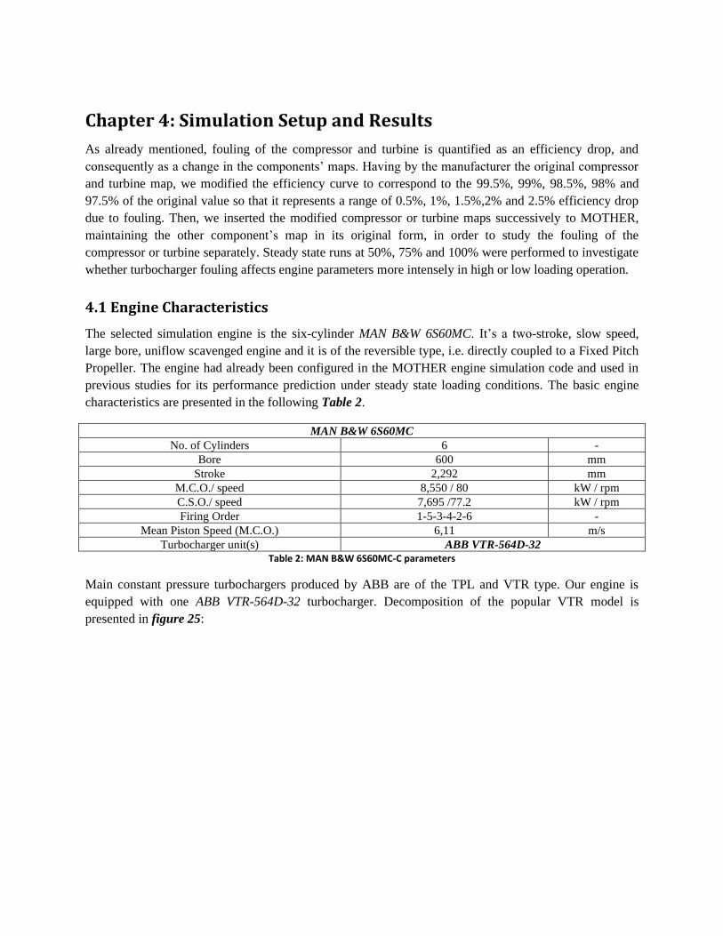
4.1 Engine Characteristics

The selected simulation engine is the six-cylinder MAN B&W 6S60MC. It’s a two-stroke, slow speed,

large bore, uniflow scavenged engine and it is of the reversible type, i.e. directly coupled to a Fixed Pitch

Propeller. The engine had already been configured in the MOTHER engine simulation code and used in

previous studies for its performance prediction under steady state loading conditions. The basic engine

characteristics are presented in the following Table 2.

MAN B&W 6S60MC

No. of Cylinders 6 -

Bore 600 mm

Stroke 2,292 mm

M.C.O./ speed 8,550 / 80 kW / rpm

C.S.O./ speed 7,695 /77.2 kW / rpm

Firing Order 1-5-3-4-2-6 -

Mean Piston Speed (M.C.O.) 6,11 m/s

Turbocharger unit(s) ABB VTR-564D-32 Table 2: MAN B&W 6S60MC-C parameters

Main constant pressure turbochargers produced by ABB are of the TPL and VTR type. Our engine is

equipped with one ABB VTR-564D-32 turbocharger. Decomposition of the popular VTR model is

presented in figure 25:

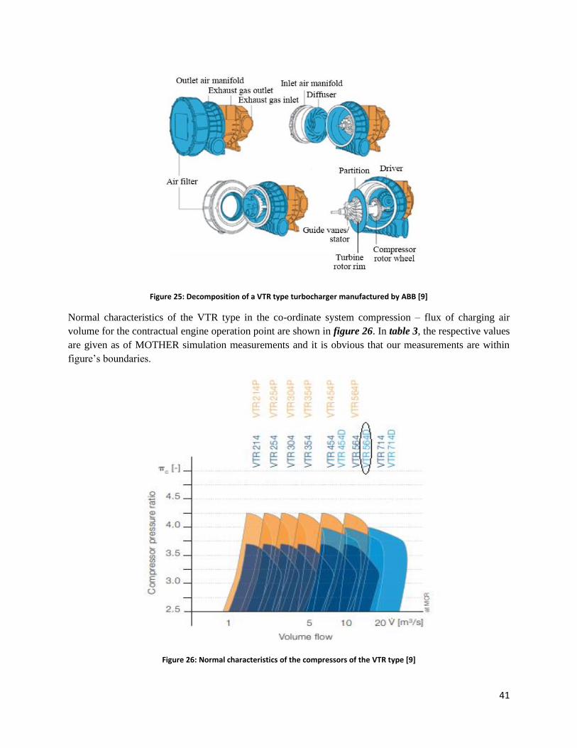
41

Figure 25: Decomposition of a VTR type turbocharger manufactured by ABB [9]

Normal characteristics of the VTR type in the co-ordinate system compression – flux of charging air

volume for the contractual engine operation point are shown in figure 26. In table 3, the respective values

are given as of MOTHER simulation measurements and it is obvious that our measurements are within

figure’s boundaries.

Figure 26: Normal characteristics of the compressors of the VTR type [9]

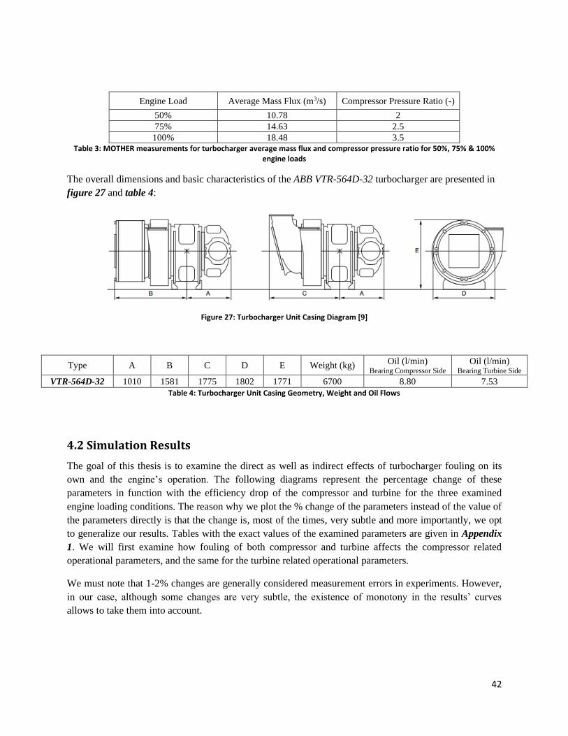
42

Engine Load Average Mass Flux (m3/s) Compressor Pressure Ratio (-)

50% 10.78 2

75% 14.63 2.5

100% 18.48 3.5 Table 3: MOTHER measurements for turbocharger average mass flux and compressor pressure ratio for 50%, 75% & 100%

engine loads

The overall dimensions and basic characteristics of the ABB VTR-564D-32 turbocharger are presented in

figure 27 and table 4:

Figure 27: Turbocharger Unit Casing Diagram [9]

Type A B C D E Weight (kg) Oil (l/min)

Bearing Compressor Side

Oil (l/min) Bearing Turbine Side

VTR-564D-32 1010 1581 1775 1802 1771 6700 8.80 7.53

Table 4: Turbocharger Unit Casing Geometry, Weight and Oil Flows

4.2 Simulation Results

The goal of this thesis is to examine the direct as well as indirect effects of turbocharger fouling on its

own and the engine’s operation. The following diagrams represent the percentage change of these

parameters in function with the efficiency drop of the compressor and turbine for the three examined

engine loading conditions. The reason why we plot the % change of the parameters instead of the value of

the parameters directly is that the change is, most of the times, very subtle and more importantly, we opt

to generalize our results. Tables with the exact values of the examined parameters are given in Appendix

1. We will first examine how fouling of both compressor and turbine affects the compressor related

operational parameters, and the same for the turbine related operational parameters.

We must note that 1-2% changes are generally considered measurement errors in experiments. However,

in our case, although some changes are very subtle, the existence of monotony in the results’ curves

allows to take them into account.

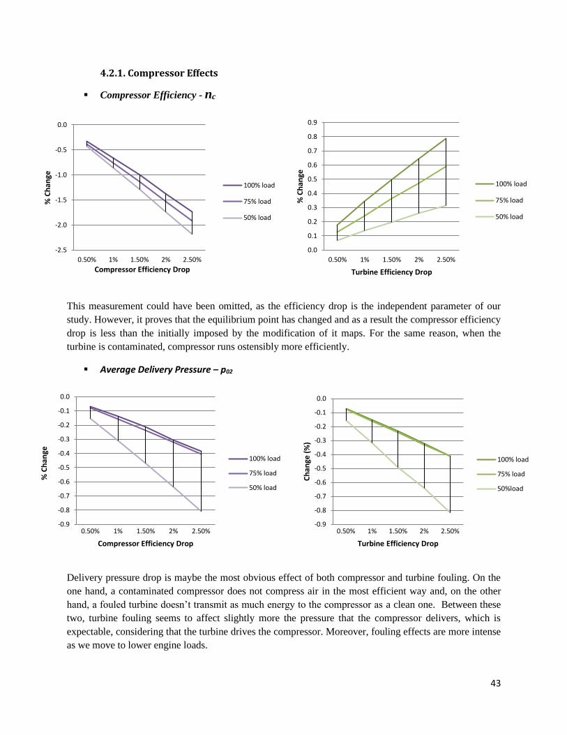
43

4.2.1. Compressor Effects

▪ Compressor Efficiency - nc

This measurement could have been omitted, as the efficiency drop is the independent parameter of our

study. However, it proves that the equilibrium point has changed and as a result the compressor efficiency

drop is less than the initially imposed by the modification of it maps. For the same reason, when the

turbine is contaminated, compressor runs ostensibly more efficiently.

▪ Average Delivery Pressure – p02

Delivery pressure drop is maybe the most obvious effect of both compressor and turbine fouling. On the

one hand, a contaminated compressor does not compress air in the most efficient way and, on the other

hand, a fouled turbine doesn’t transmit as much energy to the compressor as a clean one. Between these

two, turbine fouling seems to affect slightly more the pressure that the compressor delivers, which is

expectable, considering that the turbine drives the compressor. Moreover, fouling effects are more intense

as we move to lower engine loads.

-2.5

-2.0

-1.5

-1.0

-0.5

0.0

0.50% 1% 1.50% 2% 2.50%

% C

han

ge

Compressor Efficiency Drop

100% load

75% load

50% load

0.0

0.1

0.2

0.3

0.4

0.5

0.6

0.7

0.8

0.9

0.50% 1% 1.50% 2% 2.50%

% C

han

ge

Turbine Efficiency Drop

100% load

75% load

50% load

-0.9

-0.8

-0.7

-0.6

-0.5

-0.4

-0.3

-0.2

-0.1

0.0

0.50% 1% 1.50% 2% 2.50%

% C

han

ge

Compressor Efficiency Drop

100% load

75% load

50% load

-0.9

-0.8

-0.7

-0.6

-0.5

-0.4

-0.3

-0.2

-0.1

0.0

0.50% 1% 1.50% 2% 2.50%

Ch

ange

(%

)

Turbine Efficiency Drop

100% load

75% load

50%load

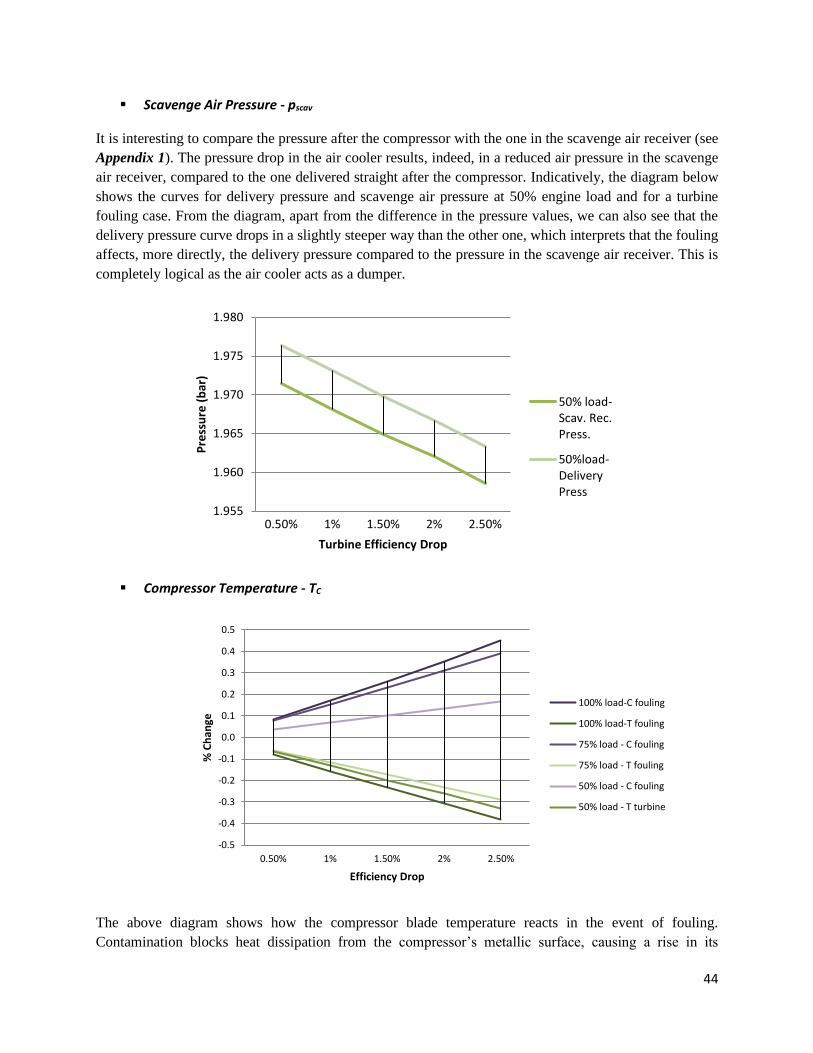
44

▪ Scavenge Air Pressure - pscav

It is interesting to compare the pressure after the compressor with the one in the scavenge air receiver (see

Appendix 1). The pressure drop in the air cooler results, indeed, in a reduced air pressure in the scavenge

air receiver, compared to the one delivered straight after the compressor. Indicatively, the diagram below

shows the curves for delivery pressure and scavenge air pressure at 50% engine load and for a turbine

fouling case. From the diagram, apart from the difference in the pressure values, we can also see that the

delivery pressure curve drops in a slightly steeper way than the other one, which interprets that the fouling

affects, more directly, the delivery pressure compared to the pressure in the scavenge air receiver. This is

completely logical as the air cooler acts as a dumper.

▪ Compressor Temperature - TC

The above diagram shows how the compressor blade temperature reacts in the event of fouling.

Contamination blocks heat dissipation from the compressor’s metallic surface, causing a rise in its

1.955

1.960

1.965

1.970

1.975

1.980

0.50% 1% 1.50% 2% 2.50%

Pre

ssu

re (

bar

)

Turbine Efficiency Drop

50% load-Scav. Rec.Press.

50%load-DeliveryPress

-0.5

-0.4

-0.3

-0.2

-0.1

0.0

0.1

0.2

0.3

0.4

0.5

0.50% 1% 1.50% 2% 2.50%

% C

han

ge

Efficiency Drop

100% load-C fouling

100% load-T fouling

75% load - C fouling

75% load - T fouling

50% load - C fouling

50% load - T turbine

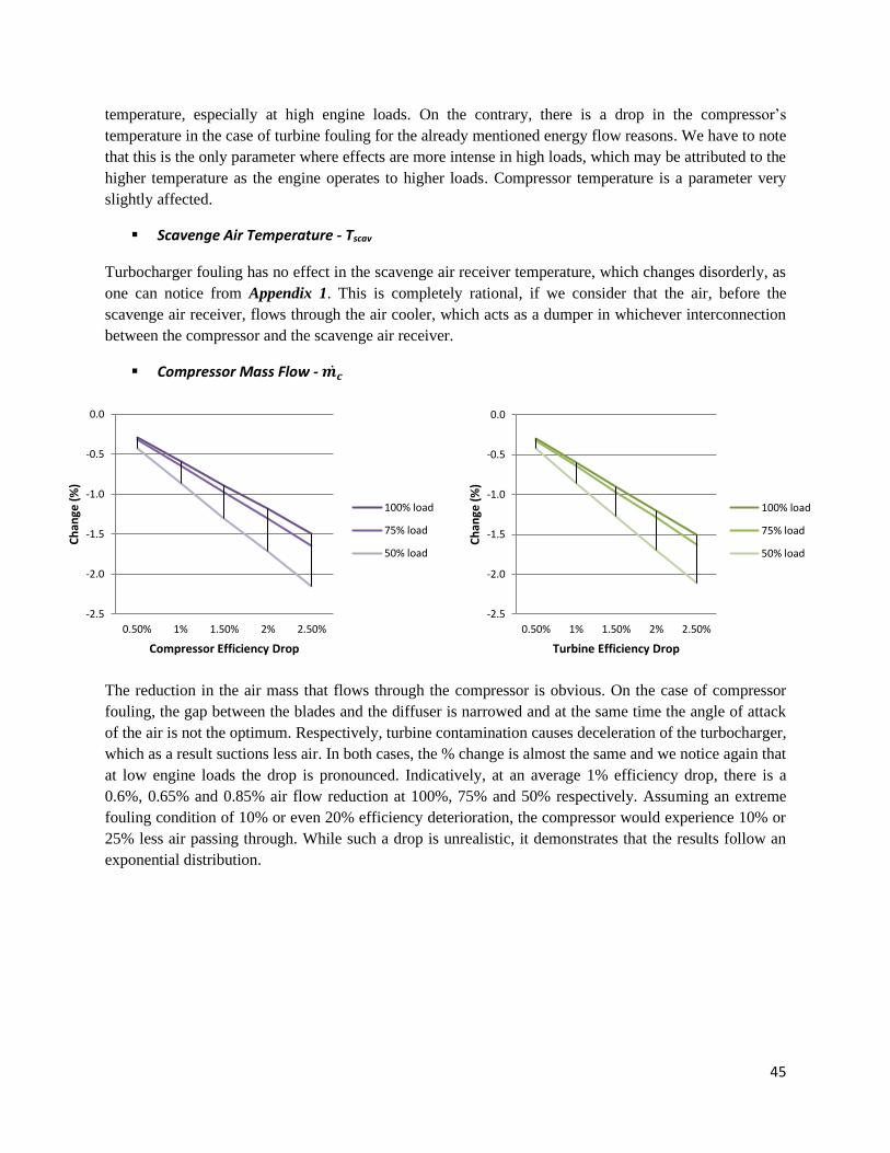
45

temperature, especially at high engine loads. On the contrary, there is a drop in the compressor’s

temperature in the case of turbine fouling for the already mentioned energy flow reasons. We have to note

that this is the only parameter where effects are more intense in high loads, which may be attributed to the

higher temperature as the engine operates to higher loads. Compressor temperature is a parameter very

slightly affected.

▪ Scavenge Air Temperature - Tscav

Turbocharger fouling has no effect in the scavenge air receiver temperature, which changes disorderly, as

one can notice from Appendix 1. This is completely rational, if we consider that the air, before the

scavenge air receiver, flows through the air cooler, which acts as a dumper in whichever interconnection

between the compressor and the scavenge air receiver.

▪ Compressor Mass Flow - 𝒎𝒄̇

The reduction in the air mass that flows through the compressor is obvious. On the case of compressor

fouling, the gap between the blades and the diffuser is narrowed and at the same time the angle of attack

of the air is not the optimum. Respectively, turbine contamination causes deceleration of the turbocharger,

which as a result suctions less air. In both cases, the % change is almost the same and we notice again that

at low engine loads the drop is pronounced. Indicatively, at an average 1% efficiency drop, there is a

0.6%, 0.65% and 0.85% air flow reduction at 100%, 75% and 50% respectively. Assuming an extreme

fouling condition of 10% or even 20% efficiency deterioration, the compressor would experience 10% or

25% less air passing through. While such a drop is unrealistic, it demonstrates that the results follow an

exponential distribution.

-2.5

-2.0

-1.5

-1.0

-0.5

0.0

0.50% 1% 1.50% 2% 2.50%

Ch

ange

(%

)

Compressor Efficiency Drop

100% load

75% load

50% load

-2.5

-2.0

-1.5

-1.0

-0.5

0.0

0.50% 1% 1.50% 2% 2.50%

Ch

ange

(%

)

Turbine Efficiency Drop

100% load

75% load

50% load

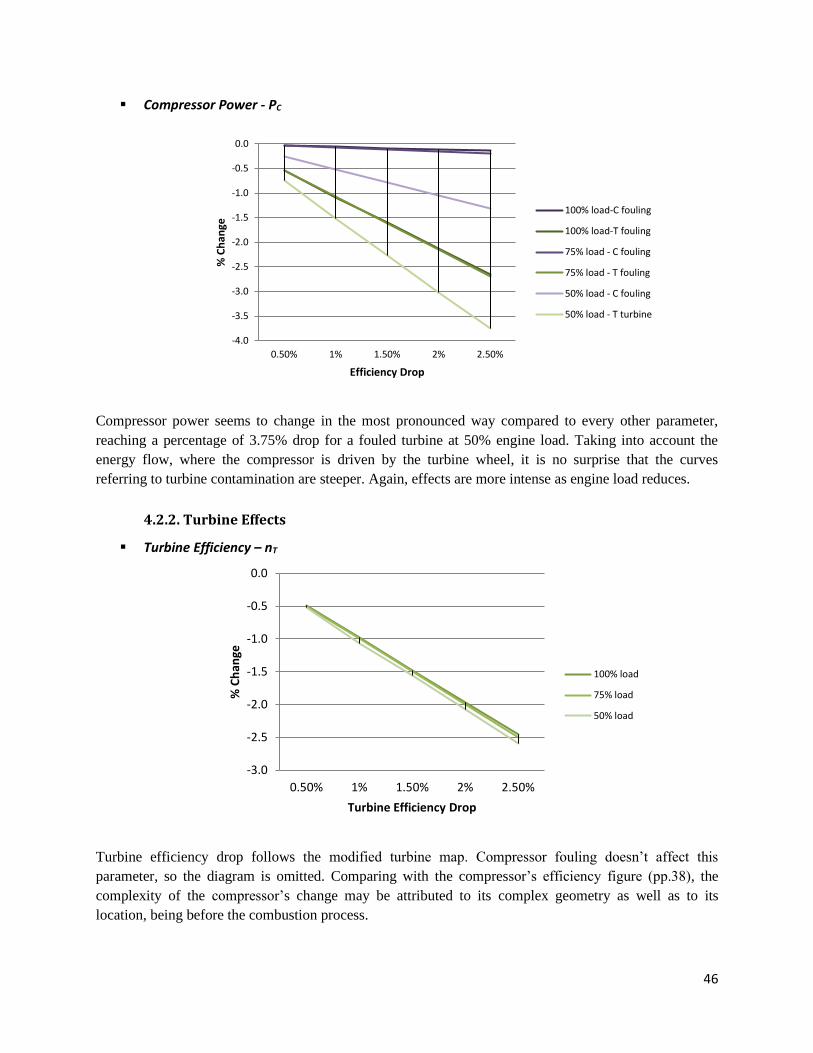
46

▪ Compressor Power - PC

Compressor power seems to change in the most pronounced way compared to every other parameter,

reaching a percentage of 3.75% drop for a fouled turbine at 50% engine load. Taking into account the

energy flow, where the compressor is driven by the turbine wheel, it is no surprise that the curves

referring to turbine contamination are steeper. Again, effects are more intense as engine load reduces.

4.2.2. Turbine Effects

▪ Turbine Efficiency – nT

Turbine efficiency drop follows the modified turbine map. Compressor fouling doesn’t affect this

parameter, so the diagram is omitted. Comparing with the compressor’s efficiency figure (pp.38), the

complexity of the compressor’s change may be attributed to its complex geometry as well as to its

location, being before the combustion process.

-4.0

-3.5

-3.0

-2.5

-2.0

-1.5

-1.0

-0.5

0.0

0.50% 1% 1.50% 2% 2.50%

% C

han

ge

Efficiency Drop

100% load-C fouling

100% load-T fouling

75% load - C fouling

75% load - T fouling

50% load - C fouling

50% load - T turbine

-3.0

-2.5

-2.0

-1.5

-1.0

-0.5

0.0

0.50% 1% 1.50% 2% 2.50%

% C

han

ge

Turbine Efficiency Drop

100% load

75% load

50% load

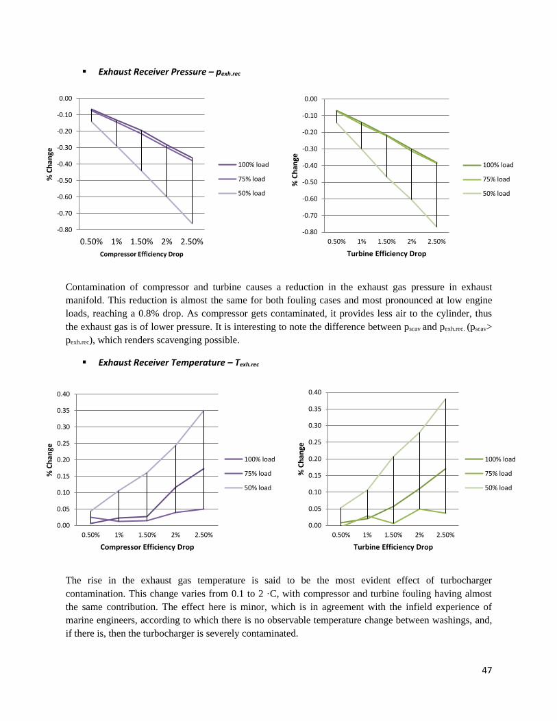
47

▪ Exhaust Receiver Pressure – pexh.rec

Contamination of compressor and turbine causes a reduction in the exhaust gas pressure in exhaust

manifold. This reduction is almost the same for both fouling cases and most pronounced at low engine

loads, reaching a 0.8% drop. As compressor gets contaminated, it provides less air to the cylinder, thus

the exhaust gas is of lower pressure. It is interesting to note the difference between pscav and pexh.rec. (pscav>

pexh.rec), which renders scavenging possible.

▪ Exhaust Receiver Temperature – Texh.rec

The rise in the exhaust gas temperature is said to be the most evident effect of turbocharger

contamination. This change varies from 0.1 to 2 ·C, with compressor and turbine fouling having almost

the same contribution. The effect here is minor, which is in agreement with the infield experience of

marine engineers, according to which there is no observable temperature change between washings, and,

if there is, then the turbocharger is severely contaminated.

-0.80

-0.70

-0.60

-0.50

-0.40

-0.30

-0.20

-0.10

0.00

0.50% 1% 1.50% 2% 2.50%

% C

han

ge

Compressor Efficiency Drop

100% load

75% load

50% load

-0.80

-0.70

-0.60

-0.50

-0.40

-0.30

-0.20

-0.10

0.00

0.50% 1% 1.50% 2% 2.50%

% C

han

ge

Turbine Efficiency Drop

100% load

75% load

50% load

0.00

0.05

0.10

0.15

0.20

0.25

0.30

0.35

0.40

0.50% 1% 1.50% 2% 2.50%

% C

han

ge

Compressor Efficiency Drop

100% load

75% load

50% load

0.00

0.05

0.10

0.15

0.20

0.25

0.30

0.35

0.40

0.50% 1% 1.50% 2% 2.50%

% C

han

ge

Turbine Efficiency Drop

100% load

75% load

50% load

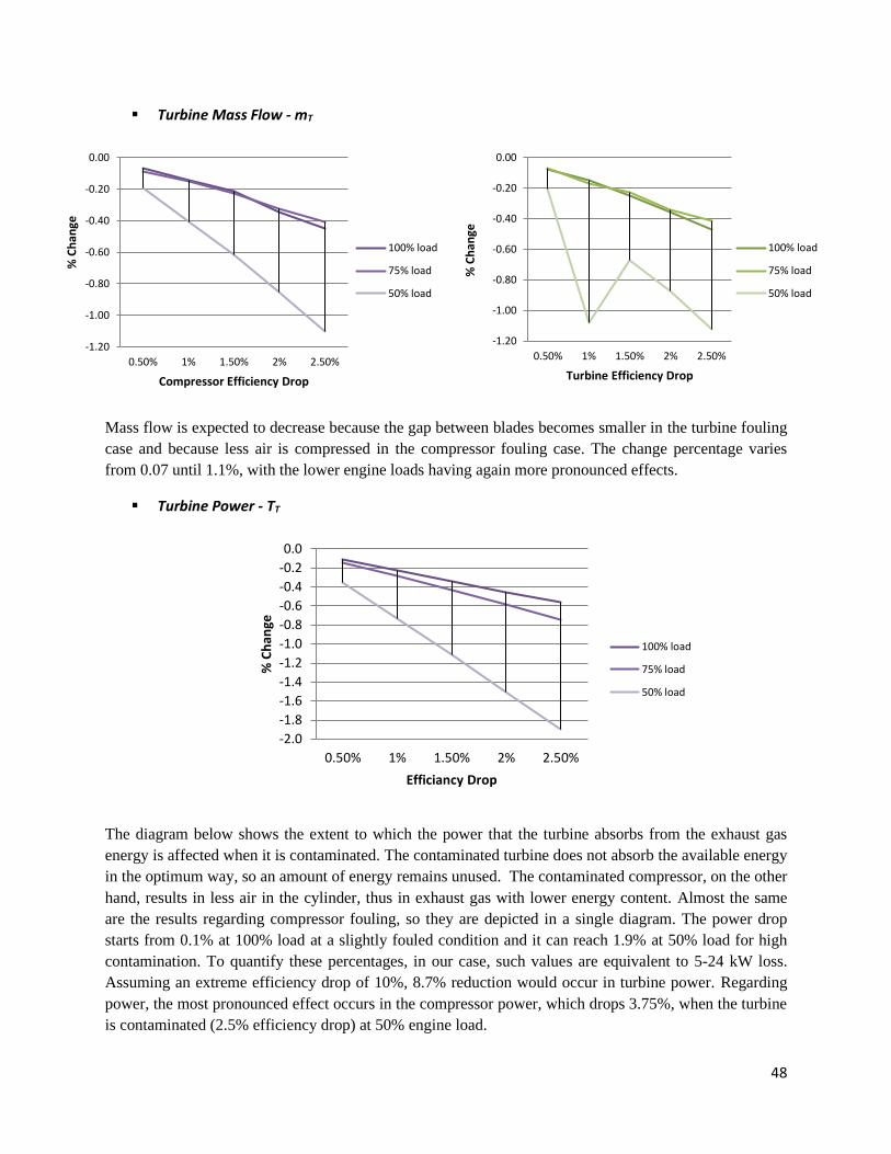
48

▪ Turbine Mass Flow - mT

Mass flow is expected to decrease because the gap between blades becomes smaller in the turbine fouling

case and because less air is compressed in the compressor fouling case. The change percentage varies

from 0.07 until 1.1%, with the lower engine loads having again more pronounced effects.

▪ Turbine Power - TT

The diagram below shows the extent to which the power that the turbine absorbs from the exhaust gas

energy is affected when it is contaminated. The contaminated turbine does not absorb the available energy

in the optimum way, so an amount of energy remains unused. The contaminated compressor, on the other

hand, results in less air in the cylinder, thus in exhaust gas with lower energy content. Almost the same

are the results regarding compressor fouling, so they are depicted in a single diagram. The power drop

starts from 0.1% at 100% load at a slightly fouled condition and it can reach 1.9% at 50% load for high

contamination. To quantify these percentages, in our case, such values are equivalent to 5-24 kW loss.

Assuming an extreme efficiency drop of 10%, 8.7% reduction would occur in turbine power. Regarding

power, the most pronounced effect occurs in the compressor power, which drops 3.75%, when the turbine

is contaminated (2.5% efficiency drop) at 50% engine load.

-1.20

-1.00

-0.80

-0.60

-0.40

-0.20

0.00

0.50% 1% 1.50% 2% 2.50%

% C

han

ge

Compressor Efficiency Drop

100% load

75% load

50% load

-1.20

-1.00

-0.80

-0.60

-0.40

-0.20

0.00

0.50% 1% 1.50% 2% 2.50%

% C

han

ge

Turbine Efficiency Drop

100% load

75% load

50% load

-2.0

-1.8

-1.6

-1.4

-1.2

-1.0

-0.8

-0.6

-0.4

-0.2

0.0

0.50% 1% 1.50% 2% 2.50%

% C

han

ge

Efficiancy Drop

100% load

75% load

50% load

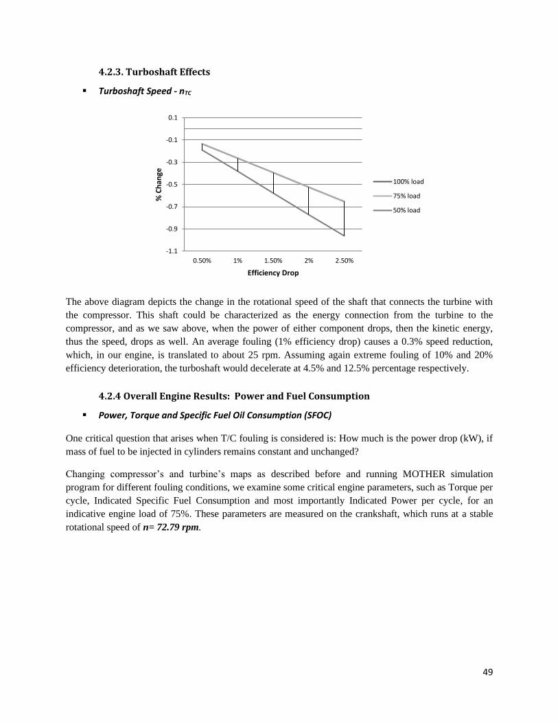
49

4.2.3. Turboshaft Effects

▪ Turboshaft Speed - nTC

The above diagram depicts the change in the rotational speed of the shaft that connects the turbine with

the compressor. This shaft could be characterized as the energy connection from the turbine to the

compressor, and as we saw above, when the power of either component drops, then the kinetic energy,

thus the speed, drops as well. An average fouling (1% efficiency drop) causes a 0.3% speed reduction,

which, in our engine, is translated to about 25 rpm. Assuming again extreme fouling of 10% and 20%

efficiency deterioration, the turboshaft would decelerate at 4.5% and 12.5% percentage respectively.

4.2.4 Overall Engine Results: Power and Fuel Consumption

▪ Power, Torque and Specific Fuel Oil Consumption (SFOC)

One critical question that arises when T/C fouling is considered is: How much is the power drop (kW), if

mass of fuel to be injected in cylinders remains constant and unchanged?

Changing compressor’s and turbine’s maps as described before and running MOTHER simulation

program for different fouling conditions, we examine some critical engine parameters, such as Torque per

cycle, Indicated Specific Fuel Consumption and most importantly Indicated Power per cycle, for an

indicative engine load of 75%. These parameters are measured on the crankshaft, which runs at a stable

rotational speed of n= 72.79 rpm.

-1.1

-0.9

-0.7

-0.5

-0.3

-0.1

0.1

0.50% 1% 1.50% 2% 2.50%

% C

han

ge

Efficiency Drop

100% load

75% load

50% load

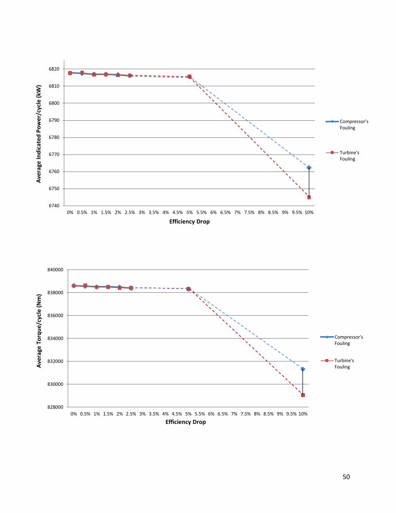
50

6740

6750

6760

6770

6780

6790

6800

6810

6820

0% 0.5% 1% 1.5% 2% 2.5% 3% 3.5% 4% 4.5% 5% 5.5% 6% 6.5% 7% 7.5% 8% 8.5% 9% 9.5% 10%

Ave

rage

In

dic

ate

d P

ow

er/

cycl

e (

kW)

Efficiency Drop

Compressor'sFouling

Turbine'sFouling

828000

830000

832000

834000

836000

838000

840000

0% 0.5% 1% 1.5% 2% 2.5% 3% 3.5% 4% 4.5% 5% 5.5% 6% 6.5% 7% 7.5% 8% 8.5% 9% 9.5% 10%

Ave

rage

To

rqu

e/c

ycle

(N

m)

Efficiency Drop

Compressor'sFouling

Turbine'sFouling

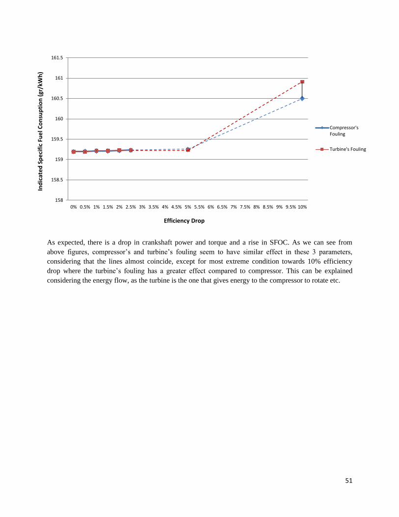
51

As expected, there is a drop in crankshaft power and torque and a rise in SFOC. As we can see from

above figures, compressor’s and turbine’s fouling seem to have similar effect in these 3 parameters,

considering that the lines almost coincide, except for most extreme condition towards 10% efficiency

drop where the turbine’s fouling has a greater effect compared to compressor. This can be explained

considering the energy flow, as the turbine is the one that gives energy to the compressor to rotate etc.

158

158.5

159

159.5

160

160.5

161

161.5

0% 0.5% 1% 1.5% 2% 2.5% 3% 3.5% 4% 4.5% 5% 5.5% 6% 6.5% 7% 7.5% 8% 8.5% 9% 9.5% 10%

Ind

icat

ed

Sp

eci

fic

Fue

l Co

nsu

pti

on

(gr

/kW

h)

Efficiency Drop

Compressor'sFouling

Turbine's Fouling

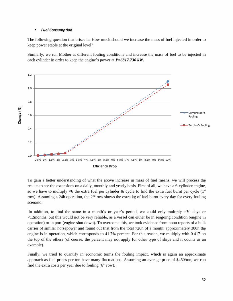
52

▪ Fuel Consumption

The following question that arises is: How much should we increase the mass of fuel injected in order to

keep power stable at the original level?

Similarly, we run Mother at different fouling conditions and increase the mass of fuel to be injected in

each cylinder in order to keep the engine’s power at P=6817.730 kW.

To gain a better understanding of what the above increase in mass of fuel means, we will process the

results to see the extensions on a daily, monthly and yearly basis. First of all, we have a 6-cylinder engine,

so we have to multiply ×6 the extra fuel per cylinder & cycle to find the extra fuel burnt per cycle (1st

row). Assuming a 24h operation, the 2nd row shows the extra kg of fuel burnt every day for every fouling

scenario.

In addition, to find the same in a month’s or year’s period, we could only multiply ×30 days or

×12months, but this would not be very reliable, as a vessel can either be in seagoing condition (engine in

operation) or in port (engine shut down). To overcome this, we took evidence from noon reports of a bulk

carrier of similar horsepower and found out that from the total 720h of a month, approximately 300h the

engine is in operation, which corresponds to 41.7% percent. For this reason, we multiply with 0.417 on

the top of the others (of course, the percent may not apply for other type of ships and it counts as an

example).

Finally, we tried to quantify in economic terms the fouling impact, which is again an approximate

approach as fuel prices per ton have many fluctuations. Assuming an average price of $450/ton, we can

find the extra costs per year due to fouling (6th row).

0.0

0.2

0.4

0.6

0.8

1.0

1.2

0.5% 1% 1.5% 2% 2.5% 3% 3.5% 4% 4.5% 5% 5.5% 6% 6.5% 7% 7.5% 8% 8.5% 9% 9.5% 10%

Ch

ange

(%

)

Efficiency Drop

Compressor'sFouling

Turbine's Fouling

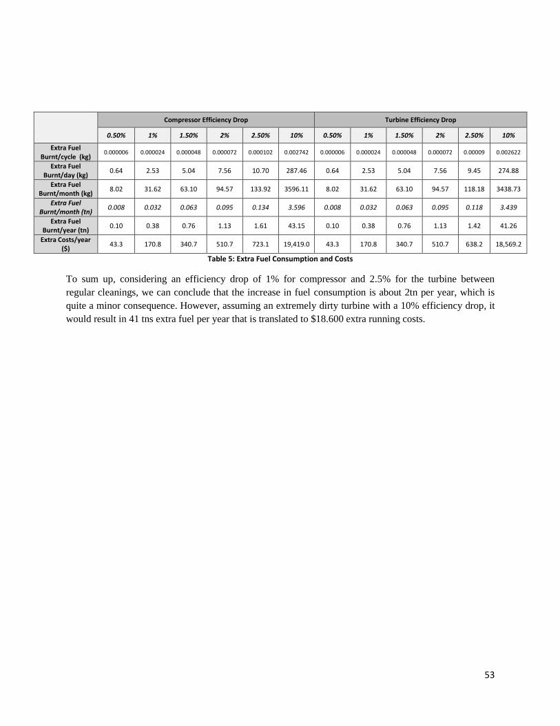
53

Compressor Efficiency Drop Turbine Efficiency Drop

0.50% 1% 1.50% 2% 2.50% 10% 0.50% 1% 1.50% 2% 2.50% 10%

Extra Fuel Burnt/cycle (kg)

0.000006 0.000024 0.000048 0.000072 0.000102 0.002742 0.000006 0.000024 0.000048 0.000072 0.00009 0.002622

Extra Fuel Burnt/day (kg)

0.64 2.53 5.04 7.56 10.70 287.46 0.64 2.53 5.04 7.56 9.45 274.88

Extra Fuel Burnt/month (kg)

8.02 31.62 63.10 94.57 133.92 3596.11 8.02 31.62 63.10 94.57 118.18 3438.73

Extra Fuel Burnt/month (tn)

0.008 0.032 0.063 0.095 0.134 3.596 0.008 0.032 0.063 0.095 0.118 3.439

Extra Fuel Burnt/year (tn)

0.10 0.38 0.76 1.13 1.61 43.15 0.10 0.38 0.76 1.13 1.42 41.26

Extra Costs/year ($)

43.3 170.8 340.7 510.7 723.1 19,419.0 43.3 170.8 340.7 510.7 638.2 18,569.2

Table 5: Extra Fuel Consumption and Costs

To sum up, considering an efficiency drop of 1% for compressor and 2.5% for the turbine between

regular cleanings, we can conclude that the increase in fuel consumption is about 2tn per year, which is

quite a minor consequence. However, assuming an extremely dirty turbine with a 10% efficiency drop, it

would result in 41 tns extra fuel per year that is translated to $18.600 extra running costs.

54

Chapter 5: Conclusions

5.1 Discussion

The aim of the present thesis was to quantify turbocharger’s fouling in the form of percentage efficiency

drop (%) between cleaning procedures and to investigate the effects of fouling on compressor, turbine and

overall engine operational parameters.

Little information was available regarding the efficiency reduction and hence, the change of efficiency

curve in compressor and turbine map, so we had to depend mainly on operator’s experience and on only a

few papers’ information on the subject. The two sides agreed that this drop is low, varying from 0.5% to

2.5%, as the periodic cleaning procedures are very well established and incorporated in engines

maintenance routine, and as a result compressor and turbine are not ‘left’ to get severely dirty.

The main findings suggest that most of the examined parameters change in the same way for the

compressor and turbine fouling, which was anticipated, as they are directly connected. In some cases,

turbine fouling has a slightly more pronounced effect, as it is the one which absorbs exhaust gas energy

and drives the compressor. Generally, considering that the turbine gets more contaminated, and thus,

suffers a greater efficiency drop, the effects of turbine fouling are greater compared to the ones of

compressor fouling. In addition, apart from compressor temperature, parameters experience a bigger

change in lower engine loads.

Another aim of this research was to identify parameters that would serve as turbocharger fouling

indicators for operators. Overall, the changes are sometimes so subtle that cannot be identified, with the

accuracy of the available on-board measuring devices (Appendix 2). Another major difficulty is that most

of the examined parameters are influenced by numerous factors and cannot serve as clear turbo fouling

indicators. The ease and accuracy of the pick-up sensor renders turboshaft rotational speed, the main

indicator when examining the possibility of fouling in turbocharger.

In general, and as already mentioned, the effects resulting from MOTHER simulation show quite subtle

changes in the values of the different parameters. This was anticipated considering the minority of the

efficiency reduction and taking into account that efficiency is only one of the many influencing

turbocharger parameters. Comparing our results regarding i.e. delivery pressure with the ones given by

manufacturers in figure 15, there is a deviation, as manufacturer demonstrates 1% drop in delivery

pressure between washings, while we found a maximum 0.8% delivery pressure drop at 50% engine load.

An obvious explanation to this is that our study is constrained to the efficiency parameter, disregarding all

the other influencing factors, such as mass flow, which is alongside reduced. Engine and turbocharger

parameters are interconnected and interdependent in a very complex manner. Isolation of one

phenomenon is only done in approximation.

To conclude, the existent cleaning methods and intervals seem adequate for the current operational

condition of the engine and turbocharger, as they keep turbo efficiency in a very satisfactory operational

quality. However, as protrayed, assuming a larger efficiency drop of 10% or 20%, the examined

parameters follow an exponential deterioration, that would severely disturb the engine’s operation. The

importance of cleaning, especially on the turbine’s side, is understood by operators, who apply all the

55

necessary cleaning procedures to protect the turbocharger and engine from damage and performance

deterioration.

5.2 Recommendations for Future Research

Fouling is a multidimensional problem depending on environment conditions, fuel oil properties and

engine combustion. For this reason, for each changed condition a different approach and research must be

made. For example, the emergency of LNG, as the ‘fuel of the future’, creates the need for new research

when it comes to its fouling capabilities and effects. Another interesting field of research has to do with

the development of coatings with anti-fouling properties, so that deposits can no longer adhere to

components’ surfaces. Of course, the use of different cleaning materials, instead of water and granules,

can improve the current cleaning methods, increasing the efficiency stability and extending the cleaning

intervals.

References

[1] V. Haueisen, T. Behr, W. Gizzi, “Turbocharger Performance Stability under HFO Conditions”,

CIMAC Paper No.170 in Congress 2010, Bergen

[2] W. Gizzi, M. Jung, P.Cellbrot, V. Haueisen, “Contamination, a challenge for turbochargers in HFO

operation”, CIMAC Paper No.176 in Congress 2007, Vienna

[3] ABB Turbocharging, “Tips for the operator”, Extracts from ABB Turbocharging’s Turbo Magazine

1990-2009, pp.6-11, 2011

[4] ABB Turbocharging, “Operating Turbochargers”, Collection of articles by Johan Schieman published

in Turbo Magazine 1992-1996, pp. 3-22

[5] N. Kyrtatos, MOtor THERmodynamics Ver 2.1- Users Manual, NTUA/LME, 2013

[6] ABB Turbo Systems Ltd, “Operation Manual VTR564D32”, 2016

[7] CIMAC, “Turbocharging Efficiencies - Definition and Guidelines for Measurements and

Calculation”, Number 27, May 2007

[8] N. Sakellaridis, D. Hountalas, “Computational Investigation of Turbocharger Performance

Degradation Effect on 2-stroke Marine Diesel Engine Performance”, CIMAC Paper No. 258 in

Congress 2013, Shanghai

[9] N. Watson, M.S. Janota, “Turbocharging the Internal Combustion Engine”, 1982

[10] ABB Turbocharging, “VTR”, Product Information, pp.5-7, 2011

[11] N.Draffin, “An Introduction to Marine Fuel Analysis”, M.I.Mar.E.S.T., Revised Edition, 2018

[12] HYUNDAI-MAN B&W, Diesel Engine Instruction Book - Maintenance Manual, Hyundai Heavy

Industries Co. LTD.

[13] A. Adamkiewicz, “An analysis of cause and effect relations in diagnostic relations of marine Diesel

engine turbocharger”, Scientific Journals-Maritime University of Szczecin, 2012

[14] M. Daiber, ABB Turbo Systems, “Embedded Turbocharger Performance Monitoring”, CIMAC

Congress 2016, Helsinki, 2016

[15] X. Cui, C. Yang, J. Ramon Serrano, M. Shi, “A performance degradation evaluation method for a

turbocharger in a diesel engine”, R. Soc. Open sci. 5:181093

[16] P. Gilge, A. Kellersmann, J. Friendrichs, J. R. Seume, “Surface Roughness of real operationally used

compressor blade and disc”, Journal of Aerospace Engineer 233(14)

[17] N. Casari, M. Pinelli, A. Suman, L. di Mare, F. Montomoli, “Gas Turbine Blade Geometry variation

due to fouling”, Proceeding of 12th Conference on Turbomachinery Fluid dynamics &

Thermodynamics ETC12, April 2017, Stockholm

[18] C. Meher-Homji, A. F. Bromley, J.-P. Stalder, “Gas Turbine Performance Deterioration and

Compressor Washing”, Proceedings of the 2nd Middle East Turbomachinery Symposium, March

2013

[19] U. Gunes, Y. Ust, A. S. Karakurt, “Performance Analysis of Turbocharged 2-Stroke Diesel Engine”,

International Conference on Engineering and Nature Science, 2015

57

[20] V. Hilakari, J. Kujala, V.V. Makinen, K. Nieminen, “A method of cleaning a charge air cooler and an

internal combustion engine”, WO 2017/114567A1 – Google Patents, 2017

[21] WARTSILA, ‘Encyclopedia of Ship Technology” by J. Babicz, Second Edition, 2015

[22] TECNOVERITAS, “Engine Performance based on Condition Monitoring Using Ship Shore Data

Connections”, by J. Antunes, R. Prackash, November 2018

[23] 2020. [Online]. Available:

https://marineandoffshoreinsight.com/crankshaft-speed-sensor-working-principle/

[24] 2020. [Online]. Available:

https://www.totallubmarine.com/faq/glossary/heavy-fuel-oil-hfo

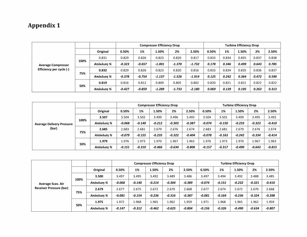
Appendix 1

Average Compressor Efficiency per cycle (-)

Compressor Efficiency Drop Turbine Efficiency Drop

Original 0.50% 1% 1.50% 2% 2.50% 0.50% 1% 1.50% 2% 2.50%

100% 0.831 0.829 0.826 0.823 0.820 0.817 0.833 0.834 0.835 0.837 0.838

Aπόκλιση % -0.323 -0.657 -1.001 -1.370 -1.732 0.178 0.346 0.499 0.643 0.785

75% 0.832 0.829 0.826 0.823 0.820 0.816 0.833 0.834 0.835 0.836 0.837

Aπόκλιση % -0.378 -0.754 -1.137 -1.526 -1.914 0.125 0.242 0.364 0.472 0.590

50% 0.819 0.816 0.812 0.809 0.805 0.802 0.820 0.821 0.821 0.822 0.822

Aπόκλιση % -0.427 -0.859 -1.289 -1.733 -2.180 0.069 0.139 0.195 0.263 0.313

Average Delivery Pressure (bar)

Compressor Efficiency Drop Turbine Efficiency Drop

Original 0.50% 1% 1.50% 2% 2.50% 0.50% 1% 1.50% 2% 2.50%

100% 3.507 3.504 3.502 3.499 3.496 3.493 3.504 3.501 3.499 3.495 3.492

Aπόκλιση % -0.068 -0.140 -0.212 -0.303 -0.387 -0.074 -0.150 -0.233 -0.323 -0.410

75% 2.685 2.683 2.681 2.679 2.676 2.674 2.683 2.681 2.679 2.676 2.674

Aπόκλιση % -0.079 -0.155 -0.235 -0.322 -0.404 -0.078 -0.163 -0.242 -0.334 -0.414

50% 1.979 1.976 1.973 1.970 1.967 1.963 1.976 1.973 1.970 1.967 1.963

Aπόκλιση % -0.151 -0.310 -0.466 -0.634 -0.806 -0.157 -0.317 -0.490 -0.643 -0.815

Average Scav. Air Receiver Pressure (bar)

Compressor Efficiency Drop Turbine Efficiency Drop

Original 0.50% 1% 1.50% 2% 2.50% 0.50% 1% 1.50% 2% 2.50%

100% 3.500 3.497 3.495 3.492 3.489 3.486 3.497 3.494 3.492 3.488 3.485

Aπόκλιση % -0.068 -0.140 -0.214 -0.304 -0.389 -0.074 -0.151 -0.232 -0.321 -0.410

75% 2.679 2.677 2.675 2.672 2.670 2.668 2.677 2.674 2.672 2.670 2.668

Aπόκλιση % -0.081 -0.154 -0.236 -0.316 -0.387 -0.081 -0.164 -0.236 -0.324 -0.398

50% 1.975 1.972 1.968 1.965 1.962 1.959 1.971 1.968 1.965 1.962 1.959

Aπόκλιση % -0.147 -0.312 -0.462 -0.625 -0.804 -0.156 -0.326 -0.490 -0.634 -0.807

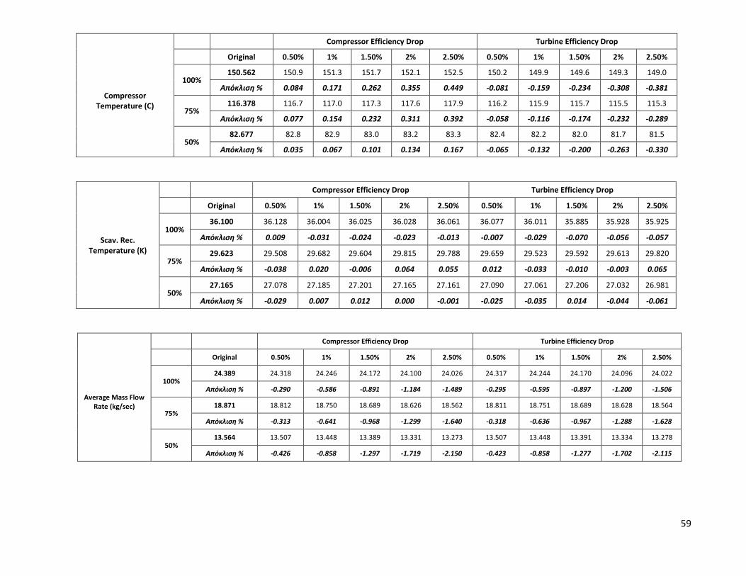
59

Compressor

Temperature (C)

Compressor Efficiency Drop Turbine Efficiency Drop

Original 0.50% 1% 1.50% 2% 2.50% 0.50% 1% 1.50% 2% 2.50%

100% 150.562 150.9 151.3 151.7 152.1 152.5 150.2 149.9 149.6 149.3 149.0

Aπόκλιση % 0.084 0.171 0.262 0.355 0.449 -0.081 -0.159 -0.234 -0.308 -0.381

75% 116.378 116.7 117.0 117.3 117.6 117.9 116.2 115.9 115.7 115.5 115.3

Aπόκλιση % 0.077 0.154 0.232 0.311 0.392 -0.058 -0.116 -0.174 -0.232 -0.289

50% 82.677 82.8 82.9 83.0 83.2 83.3 82.4 82.2 82.0 81.7 81.5

Aπόκλιση % 0.035 0.067 0.101 0.134 0.167 -0.065 -0.132 -0.200 -0.263 -0.330

Scav. Rec. Temperature (K)

Compressor Efficiency Drop Turbine Efficiency Drop

Original 0.50% 1% 1.50% 2% 2.50% 0.50% 1% 1.50% 2% 2.50%

100% 36.100 36.128 36.004 36.025 36.028 36.061 36.077 36.011 35.885 35.928 35.925

Aπόκλιση % 0.009 -0.031 -0.024 -0.023 -0.013 -0.007 -0.029 -0.070 -0.056 -0.057

75% 29.623 29.508 29.682 29.604 29.815 29.788 29.659 29.523 29.592 29.613 29.820

Aπόκλιση % -0.038 0.020 -0.006 0.064 0.055 0.012 -0.033 -0.010 -0.003 0.065

50% 27.165 27.078 27.185 27.201 27.165 27.161 27.090 27.061 27.206 27.032 26.981

Aπόκλιση % -0.029 0.007 0.012 0.000 -0.001 -0.025 -0.035 0.014 -0.044 -0.061

Average Mass Flow

Rate (kg/sec)

Compressor Efficiency Drop Turbine Efficiency Drop

Original 0.50% 1% 1.50% 2% 2.50% 0.50% 1% 1.50% 2% 2.50%

100% 24.389 24.318 24.246 24.172 24.100 24.026 24.317 24.244 24.170 24.096 24.022

Aπόκλιση % -0.290 -0.586 -0.891 -1.184 -1.489 -0.295 -0.595 -0.897 -1.200 -1.506

75% 18.871 18.812 18.750 18.689 18.626 18.562 18.811 18.751 18.689 18.628 18.564

Aπόκλιση % -0.313 -0.641 -0.968 -1.299 -1.640 -0.318 -0.636 -0.967 -1.288 -1.628

50% 13.564 13.507 13.448 13.389 13.331 13.273 13.507 13.448 13.391 13.334 13.278

Aπόκλιση % -0.426 -0.858 -1.297 -1.719 -2.150 -0.423 -0.858 -1.277 -1.702 -2.115

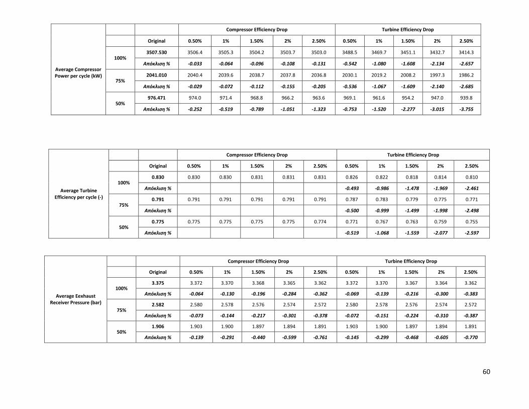
60

Average Compressor Power per cycle (kW)

Compressor Efficiency Drop Turbine Efficiency Drop

Original 0.50% 1% 1.50% 2% 2.50% 0.50% 1% 1.50% 2% 2.50%

100% 3507.530 3506.4 3505.3 3504.2 3503.7 3503.0 3488.5 3469.7 3451.1 3432.7 3414.3

Aπόκλιση % -0.033 -0.064 -0.096 -0.108 -0.131 -0.542 -1.080 -1.608 -2.134 -2.657

75% 2041.010 2040.4 2039.6 2038.7 2037.8 2036.8 2030.1 2019.2 2008.2 1997.3 1986.2

Aπόκλιση % -0.029 -0.072 -0.112 -0.155 -0.205 -0.536 -1.067 -1.609 -2.140 -2.685

50% 976.471 974.0 971.4 968.8 966.2 963.6 969.1 961.6 954.2 947.0 939.8

Aπόκλιση % -0.252 -0.519 -0.789 -1.051 -1.323 -0.753 -1.520 -2.277 -3.015 -3.755

Average Turbine Efficiency per cycle (-)

Compressor Efficiency Drop Turbine Efficiency Drop

Original 0.50% 1% 1.50% 2% 2.50% 0.50% 1% 1.50% 2% 2.50%

100% 0.830 0.830 0.830 0.831 0.831 0.831 0.826 0.822 0.818 0.814 0.810

Aπόκλιση % -0.493 -0.986 -1.478 -1.969 -2.461

75% 0.791 0.791 0.791 0.791 0.791 0.791 0.787 0.783 0.779 0.775 0.771

Aπόκλιση % -0.500 -0.999 -1.499 -1.998 -2.498

50% 0.775 0.775 0.775 0.775 0.775 0.774 0.771 0.767 0.763 0.759 0.755

Aπόκλιση % -0.519 -1.068 -1.559 -2.077 -2.597

Average Εexhaust Receiver Pressure (bar)

Compressor Efficiency Drop Turbine Efficiency Drop

Original 0.50% 1% 1.50% 2% 2.50% 0.50% 1% 1.50% 2% 2.50%

100% 3.375 3.372 3.370 3.368 3.365 3.362 3.372 3.370 3.367 3.364 3.362

Aπόκλιση % -0.064 -0.130 -0.196 -0.284 -0.362 -0.069 -0.139 -0.216 -0.300 -0.383

75% 2.582 2.580 2.578 2.576 2.574 2.572 2.580 2.578 2.576 2.574 2.572

Aπόκλιση % -0.073 -0.144 -0.217 -0.301 -0.378 -0.072 -0.151 -0.224 -0.310 -0.387

50% 1.906 1.903 1.900 1.897 1.894 1.891 1.903 1.900 1.897 1.894 1.891

Aπόκλιση % -0.139 -0.291 -0.440 -0.599 -0.761 -0.145 -0.299 -0.468 -0.605 -0.770

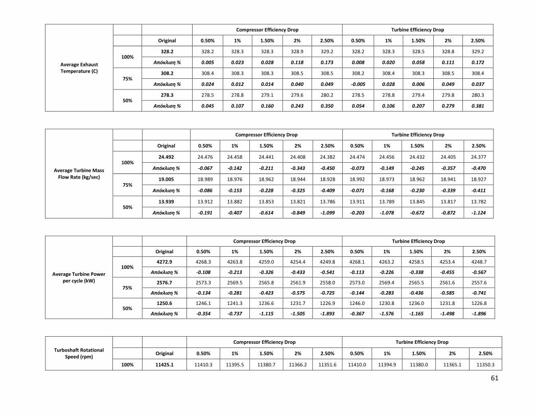
61

Average Exhaust Temperature (C)

Compressor Efficiency Drop Turbine Efficiency Drop

Original 0.50% 1% 1.50% 2% 2.50% 0.50% 1% 1.50% 2% 2.50%

100% 328.2 328.2 328.3 328.3 328.9 329.2 328.2 328.3 328.5 328.8 329.2

Aπόκλιση % 0.005 0.023 0.028 0.118 0.173 0.008 0.020 0.058 0.111 0.172

75% 308.2 308.4 308.3 308.3 308.5 308.5 308.2 308.4 308.3 308.5 308.4

Aπόκλιση % 0.024 0.012 0.014 0.040 0.049 -0.005 0.028 0.006 0.049 0.037

50% 278.3 278.5 278.8 279.1 279.6 280.2 278.5 278.8 279.4 279.8 280.3

Aπόκλιση % 0.045 0.107 0.160 0.243 0.350 0.054 0.106 0.207 0.279 0.381

Average Turbine Mass Flow Rate (kg/sec)

Compressor Efficiency Drop Turbine Efficiency Drop

Original 0.50% 1% 1.50% 2% 2.50% 0.50% 1% 1.50% 2% 2.50%

100% 24.492 24.476 24.458 24.441 24.408 24.382 24.474 24.456 24.432 24.405 24.377

Aπόκλιση % -0.067 -0.142 -0.211 -0.343 -0.450 -0.073 -0.149 -0.245 -0.357 -0.470

75% 19.005 18.989 18.976 18.962 18.944 18.928 18.992 18.973 18.962 18.941 18.927

Aπόκλιση % -0.086 -0.153 -0.228 -0.325 -0.409 -0.071 -0.168 -0.230 -0.339 -0.411

50% 13.939 13.912 13.882 13.853 13.821 13.786 13.911 13.789 13.845 13.817 13.782

Aπόκλιση % -0.191 -0.407 -0.614 -0.849 -1.099 -0.203 -1.078 -0.672 -0.872 -1.124

Average Turbine Power per cycle (kW)

Compressor Efficiency Drop Turbine Efficiency Drop

Original 0.50% 1% 1.50% 2% 2.50% 0.50% 1% 1.50% 2% 2.50%

100% 4272.9 4268.3 4263.8 4259.0 4254.4 4249.8 4268.1 4263.2 4258.5 4253.4 4248.7

Aπόκλιση % -0.108 -0.213 -0.326 -0.433 -0.541 -0.113 -0.226 -0.338 -0.455 -0.567

75% 2576.7 2573.3 2569.5 2565.8 2561.9 2558.0 2573.0 2569.4 2565.5 2561.6 2557.6

Aπόκλιση % -0.134 -0.281 -0.423 -0.575 -0.725 -0.144 -0.283 -0.436 -0.585 -0.741

50% 1250.6 1246.1 1241.3 1236.6 1231.7 1226.9 1246.0 1230.8 1236.0 1231.8 1226.8

Aπόκλιση % -0.354 -0.737 -1.115 -1.505 -1.893 -0.367 -1.576 -1.165 -1.498 -1.896

Turboshaft Rotational Speed (rpm)

Compressor Efficiency Drop Turbine Efficiency Drop

Original 0.50% 1% 1.50% 2% 2.50% 0.50% 1% 1.50% 2% 2.50%

100% 11425.1 11410.3 11395.5 11380.7 11366.2 11351.6 11410.0 11394.9 11380.0 11365.1 11350.3

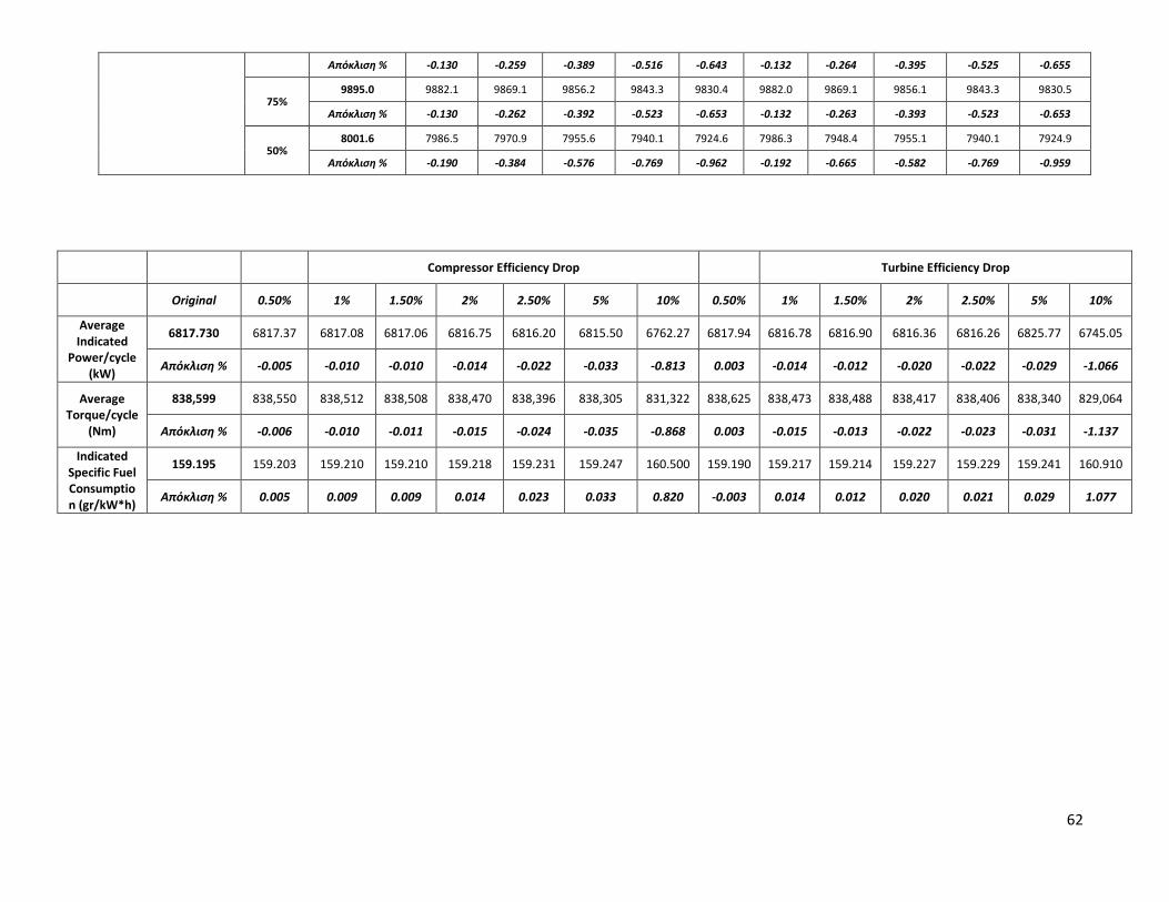
62

Aπόκλιση % -0.130 -0.259 -0.389 -0.516 -0.643 -0.132 -0.264 -0.395 -0.525 -0.655

75% 9895.0 9882.1 9869.1 9856.2 9843.3 9830.4 9882.0 9869.1 9856.1 9843.3 9830.5

Aπόκλιση % -0.130 -0.262 -0.392 -0.523 -0.653 -0.132 -0.263 -0.393 -0.523 -0.653

50% 8001.6 7986.5 7970.9 7955.6 7940.1 7924.6 7986.3 7948.4 7955.1 7940.1 7924.9

Aπόκλιση % -0.190 -0.384 -0.576 -0.769 -0.962 -0.192 -0.665 -0.582 -0.769 -0.959

Compressor Efficiency Drop Turbine Efficiency Drop

Original 0.50% 1% 1.50% 2% 2.50% 5% 10% 0.50% 1% 1.50% 2% 2.50% 5% 10%

Average Indicated

Power/cycle (kW)

6817.730 6817.37 6817.08 6817.06 6816.75 6816.20 6815.50 6762.27 6817.94 6816.78 6816.90 6816.36 6816.26 6825.77 6745.05

Aπόκλιση % -0.005 -0.010 -0.010 -0.014 -0.022 -0.033 -0.813 0.003 -0.014 -0.012 -0.020 -0.022 -0.029 -1.066

Average Torque/cycle

(Nm)

838,599 838,550 838,512 838,508 838,470 838,396 838,305 831,322 838,625 838,473 838,488 838,417 838,406 838,340 829,064

Aπόκλιση % -0.006 -0.010 -0.011 -0.015 -0.024 -0.035 -0.868 0.003 -0.015 -0.013 -0.022 -0.023 -0.031 -1.137

Indicated Specific Fuel Consumption (gr/kW*h)

159.195 159.203 159.210 159.210 159.218 159.231 159.247 160.500 159.190 159.217 159.214 159.227 159.229 159.241 160.910

Aπόκλιση % 0.005 0.009 0.009 0.014 0.023 0.033 0.820 -0.003 0.014 0.012 0.020 0.021 0.029 1.077

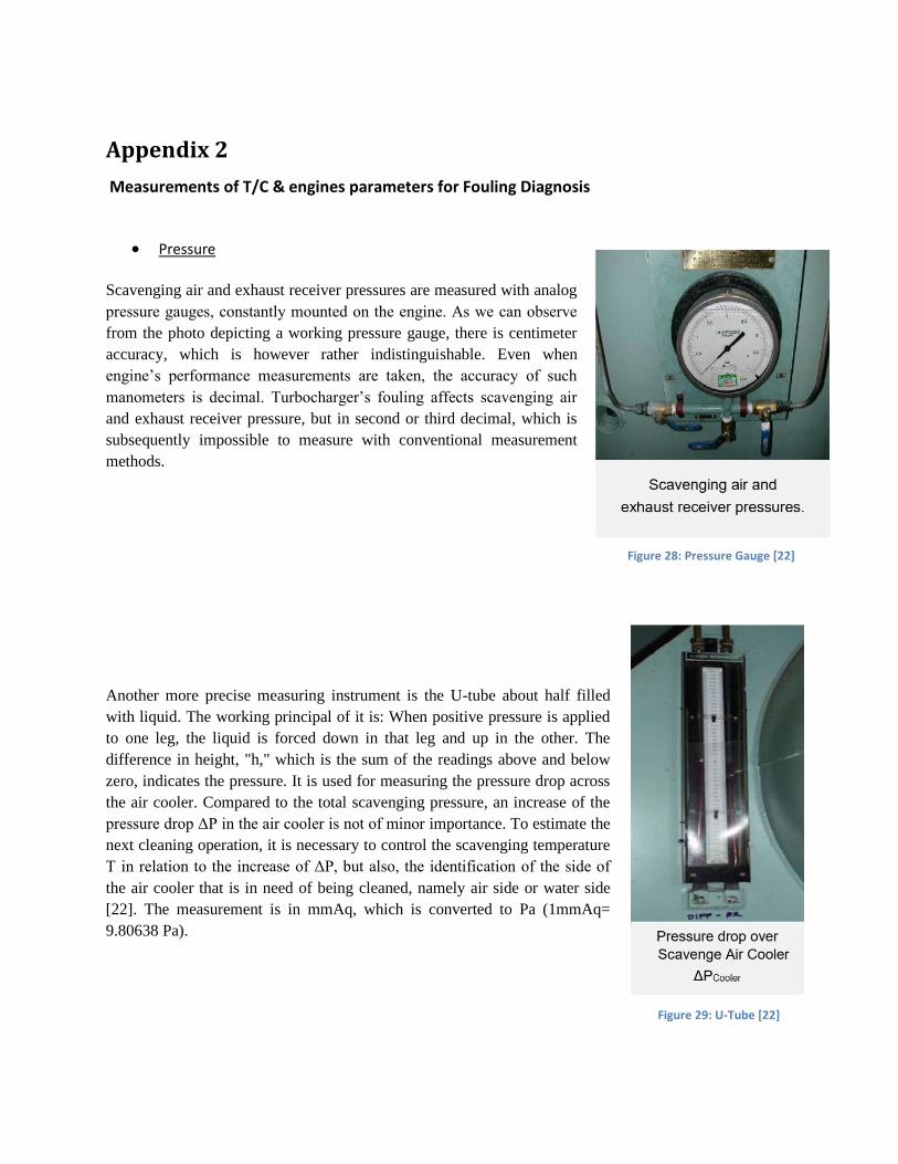
Appendix 2

Measurements of T/C & engines parameters for Fouling Diagnosis

• Pressure

Scavenging air and exhaust receiver pressures are measured with analog

pressure gauges, constantly mounted on the engine. Αs we can observe

from the photo depicting a working pressure gauge, there is centimeter

accuracy, which is however rather indistinguishable. Even when

engine’s performance measurements are taken, the accuracy of such

manometers is decimal. Turbocharger’s fouling affects scavenging air

and exhaust receiver pressure, but in second or third decimal, which is

subsequently impossible to measure with conventional measurement

methods.

Another more precise measuring instrument is the U-tube about half filled

with liquid. The working principal of it is: When positive pressure is applied

to one leg, the liquid is forced down in that leg and up in the other. The

difference in height, "h," which is the sum of the readings above and below

zero, indicates the pressure. It is used for measuring the pressure drop across

the air cooler. Compared to the total scavenging pressure, an increase of the

pressure drop ΔP in the air cooler is not of minor importance. To estimate the

next cleaning operation, it is necessary to control the scavenging temperature

T in relation to the increase of ΔP, but also, the identification of the side of

the air cooler that is in need of being cleaned, namely air side or water side

[22]. The measurement is in mmAq, which is converted to Pa (1mmAq=

9.80638 Pa).

Figure 28: Pressure Gauge [22]

Figure 29: U-Tube [22]

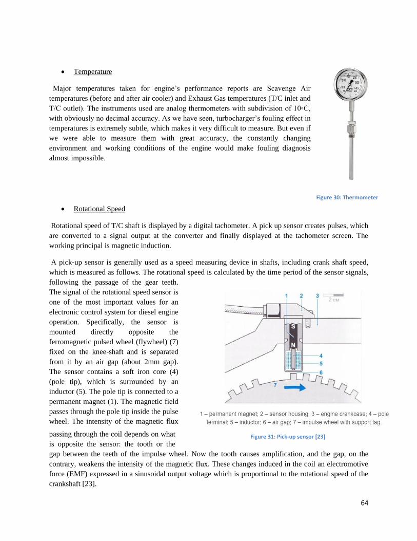
64

• Temperature

Major temperatures taken for engine’s performance reports are Scavenge Air

temperatures (before and after air cooler) and Exhaust Gas temperatures (T/C inlet and

T/C outlet). The instruments used are analog thermometers with subdivision of 10◦C,

with obviously no decimal accuracy. As we have seen, turbocharger’s fouling effect in

temperatures is extremely subtle, which makes it very difficult to measure. But even if

we were able to measure them with great accuracy, the constantly changing

environment and working conditions of the engine would make fouling diagnosis

almost impossible.

• Rotational Speed

Rotational speed of T/C shaft is displayed by a digital tachometer. A pick up sensor creates pulses, which

are converted to a signal output at the converter and finally displayed at the tachometer screen. The

working principal is magnetic induction.

A pick-up sensor is generally used as a speed measuring device in shafts, including crank shaft speed,

which is measured as follows. The rotational speed is calculated by the time period of the sensor signals,

following the passage of the gear teeth.

The signal of the rotational speed sensor is

one of the most important values for an

electronic control system for diesel engine

operation. Specifically, the sensor is

mounted directly opposite the

ferromagnetic pulsed wheel (flywheel) (7)

fixed on the knee-shaft and is separated

from it by an air gap (about 2mm gap).

The sensor contains a soft iron core (4)

(pole tip), which is surrounded by an

inductor (5). The pole tip is connected to a

permanent magnet (1). The magnetic field

passes through the pole tip inside the pulse

wheel. The intensity of the magnetic flux

passing through the coil depends on what

is opposite the sensor: the tooth or the

gap between the teeth of the impulse wheel. Now the tooth causes amplification, and the gap, on the

contrary, weakens the intensity of the magnetic flux. These changes induced in the coil an electromotive

force (EMF) expressed in a sinusoidal output voltage which is proportional to the rotational speed of the

crankshaft [23].

Figure 30: Thermometer

Figure 31: Pick-up sensor [23]

65

Due to the very high rotational speed of T/C shaft, T/C pick up sensors are simpler than the ones

described above. However, the working principle remains the same, which gives us the ability of

measuring T/C speed with sufficient accuracy, so as to make fouling diagnosis of the turbocharger. As we

have seen rpm drop varies from 10 to 70 rpm due to fouling under normal cleaning conditions, while an

approximate 500 rpm drop can be seen in extreme fouling conditions of 10% efficiency drop. This fact in

combination with the difficulty of accurately measuring other parameters (p, T, mass flow etc) as we have

already shown, makes rotational speed the most suitable diagnosis tool for T/C fouling.