The Forecasting Value of Dividend Yields within Industry Data

by

Aman Bhangu

Bachelor of Science - Major Mathematics Simon Fraser University (2001 )

Graduate Diploma in Business Administration Simon Fraser University (2003)

PROJECT SUBMITTED IN PARTIAL FULFILLMENT OF THE REQUIREMENTS FOR THE DEGREE OF

MASTER OF BUSINESS ADMINISTRATION

In the Global Asset and wealth Management Program

of the Faculty of Business Administration

O Aman Bhangu 2006

SIMON FRASER UNIVERSITY

Spring 2006

All rights reserved. This work may not be reproduced in whole or in part, by photocopy or other means, without permission of the author.

Approval

Name: Aman Bhangu

Degree: Master of Business Administration

Title of Project: The Forecasting Value of Dividend Yields within Industry Data

Examining Committee: Dr. Robert R. Grauer Senior Project Supervisor Endowed Professor

Dr. Peter Klein Second Project Supervisor Associate Professor

Date Approved:

SIMON FRASER " N I W R ~ I ~ brary

DECLARATION OF PARTIAL COPYRIGHT LICENCE

The author, whose copyright is declared on the title page of this work, has granted to Simon Fraser University the right to lend this thesis, project or extended essay to users of the Simon Fraser University Library, and to make partial or :single copies only for such users or in response to a request from the library of any other university, or other educational institution, on its own behalf or for one of its users.

The author has further granted permission to Simon Fraser University to keep or make a digital copy for use in its circulating collection, and, without changing the content, to translate the thesislproject or extended essays, if technically possible, to any medium or format for the purpose of preservation of the digital work.

The author has further agreed that permission for multiple copying of this work for scholarly purposes may be granted by either the author or the Dean of Graduate Studies.

It is understood that copying or publication of this work for financial gain shall not be allowed without the author's written perniission.

Permission for public performance, or limited permission for private scholarly use, of any multimedia materials forming part of this work, may have been granted by the author. This information may be found on the separately catalogued multimedia material and in the signed Partial Copyright Licence.

The original Partial Copyright Licence attesting to these terms, and signed by this author, may be found in the original bound copy of this work, retained in the Simon Fraser University Archive.

Simon Fraser University Library Burnaby, BC, Canada

Abstract

The economic and statistical significance of using dividend yields to forecast

future returns has been examined in numerous manners. This paper examines

the topic through a time series analysis of dis-aggregated industry returns

regressed onto aggregated equity-market dividend yields. In additiom, a trading

model is employed to further examine if any statistical significance of the

proposed relationships between dividend yields and future retu,rns can be

translated into economic significance. Economic significance is rneasured as

both absolute dollar return, as well as return per unit risk over that of industry

benchmarks.

iii

To my fiance, Jessie K, who provided me with encouragement throughout my studies.

To my parents, Romesh & Swarn Bhangu, who provided me with the foundation to undertake my studies.

And to my best friends, Ajbinder & Naveen, who made this experience enjoyable and memorable.

Acknowledgements

I would like to acknowledge Dr. Wal1:er Wattamaniuk and the entiire Office of

Analytical Studies at Simon Fraser University for keeping me gainfully employed as I

undertook this endeavour. It has been an honour and a privilege working with you all.

Table of Contents

Approval .......................................................................................................................... ii

... Abstract ......................................................................................................................... III

Dedication ...................................................................................................................... iv

Acknowledgements .......................................................................................................... v

Table of Contents ............................................................................................................. vi

List of Tables ................................................................................................................. vii

Introduction ..................................................................................................................... 1

Data ............................................................................................................................... -9

Testing Methods ............................................................................................................ I I

......................................................................................................................... Results . I 4

Regression Analysis. .............................................................................................. 14

Trading Rule - Dollar Return Analysis ..................................................................... 17

Trading Rule - Sharpe Ratio Analysis .................................................................... 23

Summary and Conclusions .......................................................................................... ..28

Appendix .......................................................... ,, ........................................................... -31

Reference List ................................................................................................................. 32

List of Tables

Table 1: Regression of Equal Weighted lndustry Return on Dividend-Yield and Risk-Free-Return .............................................................................. ., .............. 14

Table 2: Regression of Value Weighted lndustry Return on Dividend-Yield and Risk-Free-Return .............................................................................................. 15

Table 3: Regression of Value Weighted Industry Return on Dividend-Yield .................... 16

Table 4: Dollar Return Generated by Trading Model using Dividend-Yield and Risk-Free-Return Based Forecasting vs. Dollar Return of lndustry Portfolios - value weighted data ...................................................................... 18

Table 5: Dollar Return Generated by Trading-Model using Dividend-Yield Based Forecasting vs. Dollar Return of lndustry Portfolios - value weighted data .................................................................................................................. 21

Table 6: Sharpe Ratios Generated by Trading Model using Dividend-Yield and Risk-Free-Return Based Forecasting vs. Sharpe Ratios of lndustry Portfolios - value weighted data ...................................................................... 24

Table 7: Sharpe Ratios Generated by Trading Model using Dividend-Yield Based Forecasting vs. Sharpe Ratios of lndustry Portfolios - value weighted data .................................................................................................................. 26

Table A: Absolute Dollar Value Return of Investing in US 30 day Treasury Bills. ........... 31

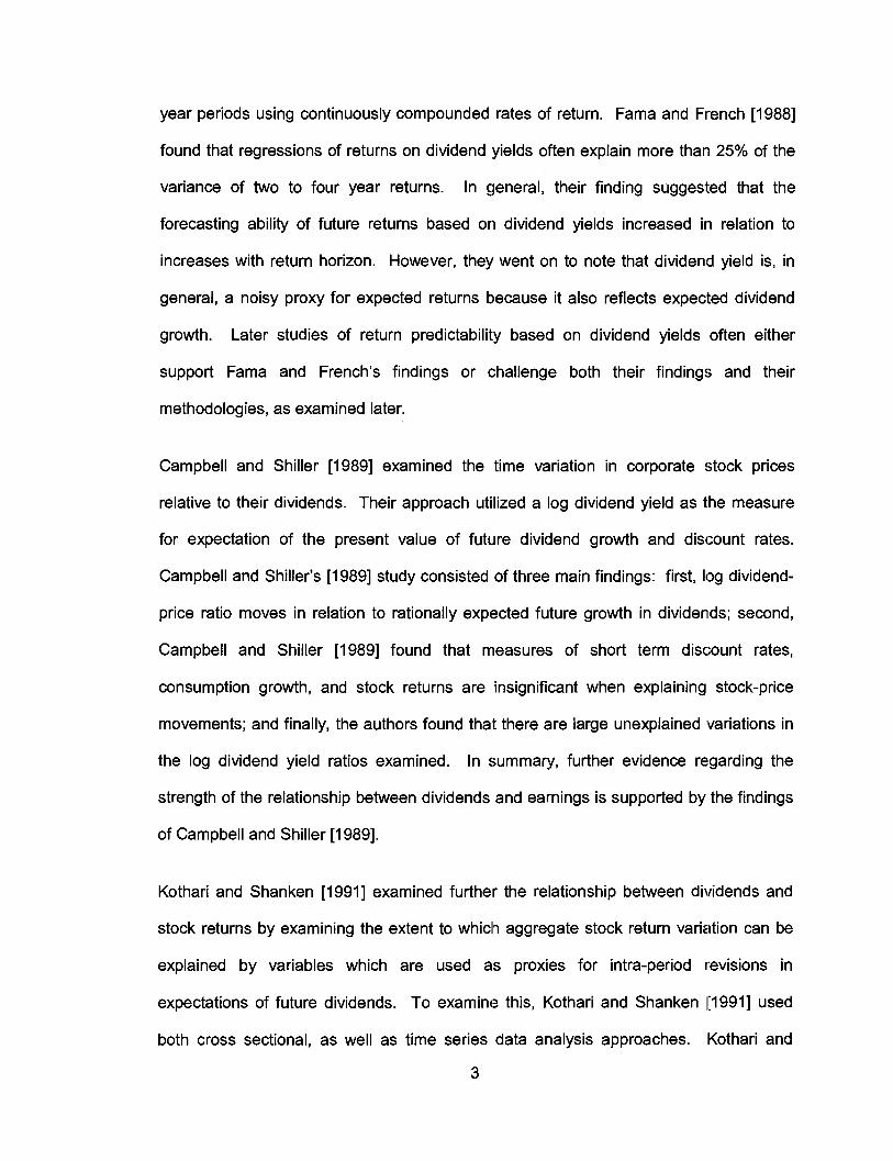
Introduction

There has been extensive discussion regarding the value of dividend yields in

forecasting future equity returns. The final conclusion as to whether or not dividend

yields do indeed possess return forecasting value is debatable. However, further

examination of this topic within disaggregated sector data may identify the market

sectors, if any, where dividend yields provide significant forecasting value. A review of

the literature concerning the value of using dividend yields in forecasting returns, as well

as other topics related to dividend yields which are relevant to the general context of the

proposed study, follow.

When examining dividend yields as a predictive indicator, an initial concern is that

dividends can be subject to relatively ad-hoc changes in dividend policy by corporate

management. Although the statistical impact of such changes is dampened when

examining aggregated data, it still warrants investigation. One of the earlier and more

relevant papers examining the impact of dividend policy on stock prices, Black and

Scholes [1974], found that corporations that increase dividends do not see a definitive

affect on stock price. Specifically, Black and Scholes [I9741 found that any temporary

change in stock price resulting from an increase in dividends would diminish if the initial

change in dividend does not correspond to a real change in expected future earnings.

Black and Scholes [I9741 thereby alleviate concerns that ad-hoc changes in dividend

policies may hinder the accuracy of equity return forecasts.

Keim [ I 9851 further addressed several topics related to dividend yields such as taxation,

firm size, stock returns, and seasonality; through his examination of NYSE data over the

period of 1931 to 1978. Among other finding!;, Keim [I9851 confirmed earlier results of

Blume [ I 9801 who found that there existed a non-linear relation between long-run yields

and returns. However, Keim [I9851 reported that the findings were dominated by the

effects of January data and that when January data was removed from the examined

data set, the relationship was no longer significant. Furthermore, Keim 119851

hypothesized that the January yield effect may be the result of the significant relationship

between January stock returns and market value of equity. It is also notable to mention

that Keim [ I 9851 examined the marginal explanatory power of dividend yields in January

data while controlling for firm size. Keim's [I19851 findings on this analysis suggested

that dividend yields and size are related to the same asset pricing factor. Furthermore,

Keim [I9851 noted a few important observatiolns between dividend yields and firm size

such as the tendency of dividend yields and firm size to be inversely related, and that the

largest firms on the NYSE are not the largest dividend yield firms, which instead tend to

be firms of "mid-size".

Fama and French [1987a] further demonstrated the importance of firm size through their

examination of autocorrelations and return predictability. Specifically, Fama and French

[1987a] found that returns are more predictable for portfolios consisting of srnaller firms.

These findings resulted from an examination olf first-order autocorrelations of returns for

industry portfolios and portfolios formed on the basis of size. In addition to their findings,

Fama and French [1987a] cited the works of King [1966], Banz [1981], andl Huberman

and Kandel [I9851 to support their assertion that firm size and industry type are

dimensions which are known to impact return behaviour.

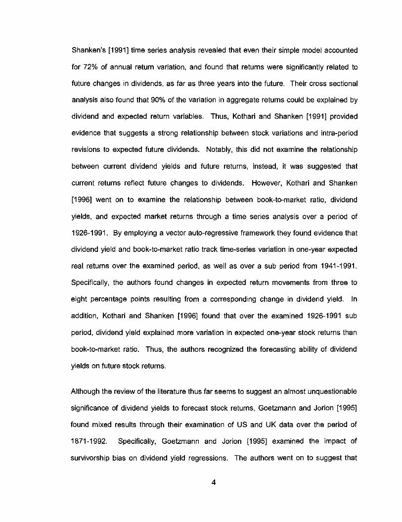
This direct examination of the effectiveness of using dividend yield in forecasting future

returns begins by reviewing the findings of Fama and French [1988]. Thik particular

study examined the use of dividend yields to forecast returns over one month to four

year periods using continuously compounded rates of return. Fama and French [I9881

found that regressions of returns on dividend yields often explain more than 25% of the

variance of two to four year returns. In general, their finding suggested that the

forecasting ability of future returns based or1 dividend yields increased in relation to

increases with return horizon. However, they went on to note that dividend yield is, in

general, a noisy proxy for expected returns because it also reflects expected dividend

growth. Later studies of return predictability based on dividend yields often either

support Fama and French's findings or challenge both their finding:; and their

methodologies, as examined later.

Campbell and Shiller [I9891 examined the time variation in corporate stock prices

relative to their dividends. Their approach utilized a log dividend yield as the measure

for expectation of the present value of future dividend growth and discount rates.

Campbell and Shiller's [ I 9891 study consisted of three main findings: first, log dividend-

price ratio moves in relation to rationally expected future growth in dividen~ds; second,

Campbell and Shiller [I9891 found that measures of short term discount rates,

consumption growth, and stock returns are insignificant when explaining stock-price

movements; and finally, the authors found that there are large unexplained ,variations in

the log dividend yield ratios examined. In summary, further evidence regarding the

strength of the relationship between dividends and earnings is supported by the findings

of Campbell and Shiller [ I 9891.

Kothari and Shanken [I9911 examined further the relationship between dividends and

stock returns by examining the extent to whiclh aggregate stock return variation can be

explained by variables which are used as proxies for intra-period revisions in

expectations of future dividends. To examine this, Kothari and Shanken 1[1991] used

both cross sectional, as well as time series data analysis approaches. Kothari and

3

Shanken's [I9911 time series analysis revealed that even their simple model accounted

for 72% of annual return variation, and found that returns were significantly related to

future changes in dividends, as far as three years into the future. Their crclss sectional

analysis also found that 90% of the variation in aggregate returns could be explained by

dividend and expected return variables. Thus, Kothari and Shanken [I9011 provided

evidence that suggests a strong relationship between stock variations and intra-period

revisions to expected future dividends. Notably, this did not examine the relationship

between current dividend yields and future returns, instead, it was suggested that

current returns reflect future changes to diviidends. However, Kothari and Shanken

[I9961 went on to examine the relationship between book-to-market ratio, dividend

yields, and expected market returns through a time series analysis over a period of

1926-1 991. By employing a vector auto-regressive framework they found evidence that

dividend yield and book-to-market ratio track 1:ime-series variation in one-year expected

real returns over the examined period, as well as over a sub period from 1941-1991.

Specifically, the authors found changes in expected return movements from three to

eight percentage points resulting from a corresponding change in dividend yield. In

addition, Kothari and Shanken [I9961 found that over the examined 1926-1991 sub

period, dividend yield explained more variation in expected one-year stock returns than

book-to-market ratio. Thus, the authors recognized the forecasting ability of dividend

yields on future stock returns.

Although the review of the literature thus far seems to suggest an almost unquestionable

significance of dividend yields to forecast stock returns, Goetzmann and Jorion [ I 9951

found mixed results through their examination of US and UK data over the period of

1871 -1 992. Specifically, Goetzmann and Jorion [ I 9951 examined the impact of

survivorship bias on dividend yield regressions. The authors went on to suggest that

mean reversion tendencies of dividend yields create the false appearance of return

predictability. After attempting to correct for the effects of survivorship bias through the

employment of a boot-strapping model, Goebmann and Jorion [I9951 concluded weak

forecasting ability existed over only some sub-periods within both the US and UK data

sets.

Wilkie [I9921 continued the discussion in a similar manner as Fama and French [I9881

but added an examination of optimal return horizon nn relation to dividend forecasting

ability. Wilkie's [I9921 findings suggested that correlation between stock returns and

dividend yields continue to heighten as return horizons increase up to ;a maximum

appearing between 70 and 80 months. This study is significant because it serves to

recognize the relationship between current dividend yields and its importance on future

returns over a defined horizon.

Hodrick [I9921 utilized three alternative measures for long return-horizon forecasting by

using Monte Carlo experiments intended to address small sample bias bellieved to be

present in preceding studies. The three alternative measures Hodrick [I99211 utilized are

as follows: first, Hodrick [ I 9921 examined forecasting future stock returns based on an

OLS regression as presented by Richardson and Smith [1991]; second, Hodrick 119921

examined forecasting future stock returns based on an OLS regression reformulation as

introduced by Jegdeesh [ I 9901; and finally, the! author examined forecasting future stock

returns based on a vector auto-regressive method as performed by Campbell and Shiller

[ I 9881. Hodrick [ I 9921 concluded that the vector auto-regressive method of Cambell

and Shiller [I9881 is the most effective method for studying long return-horizon

forecasting. Notably, this methodology was not inline with the methodology employed by

Fama and French [1988].

Harris and Sanchez-Vale [I9991 briefly exa~mined a series of five multi.variable lag

regression models, utilizing historical dividend yield, as well as dividend yield

transformations, in order to forecast future returns. Their analysis used UK equity

returns while investigating the gain from allowing equity and bond yields and lagged

yields to freely enter the proposed regression equations. The authors found little

statistical difference between the five models tested. However, when testing the models

with an out-of-sample trading strategy, Harris and Sanchez-Vale [I9991 discovered

greater profitability arising from the regression model that utilized a series of "reverse

yield gaps", defined as the difference between the consol yield and the equity dividend

yield. Thus, Harris and Sanchez-Vale [I9991 provided further support for .the value of

return forecasting through dividend yields;, as well as through dividend yield

transformations.

Wolf [2000] presented a very rich summary arid critical examination of findings from the

literature examining return forecasting from dividend yields. Specifically, Wolf [2000]

commented that the models proposed by Rozeff [1984], Campbell and Shiller [1988a],

Fama and French [1988], Nelson and Kim [I9931 and Hodrick [1992:1; contained

numerous statistical problems. In particular, Wolf [2000] noted that stock return

regressions contain strong dependency structures which result in biases within the

coefficient estimations. In fact, Wolf [2000] stated that such statistical methodologies

tend to over support the no-predictability hypothesis. Furthermore, Wolf [2000]

described Jorion's [I9931 boot-strapping methodology as not being supported by

theoretical properties. To avoid the problems of preceding studies, 'Wolf [2000]

employed a sub sampling methodology. However, he concluded that there was no

significant evidence to suggest future stock returns can be forecasted by divildend yields.

Schwert [2003] also conducted an investigation of dividend yields and their forecasting

ability. Schwert [2003] began his study through an examination of Fama and French's

[I9881 study which found a statistically significant relationship between dividend yields

and future returns. The data set used by Fama and French [I9881 covered the period

from 1927 through to 1986, however Schwerlt [I9881 expanded on this to include data

from 1872-2000. Schwert [2003] suggested that by examining this larger data set, the

findings of Fama and French [I9881 are diminished as a result of a much weaker

relation. To further examine his findings, Schwert [2003] employed an "out of sample"

trading strategy which invests in either a completely short-term bond portfolio or entirely

in an equity portfolio. Notably, Schwert [2003] only used regression parameters derived

from the original 1927-1986 Fama French [I9881 data set to test his trading model over

a period of 1872-2000. Thus, Schwert's [2003] criticism of the use of dividend yields to

forecast returns may not be as justifiable as it initially appeared.

In summary, this brief review of the literature demonstrates the differing opinions and

research findings with regards to the predictive ability of dividend yields in forecasting

future rates of return. This paper continues the discussion by utilizing a similar

methodology to that of Fama and French [I9881 by examining aggregated dividend

yields in the US market place and their ability to forecast disaggregated industry returns

for 12 US sub-industries.

The innovation of the methods proposed here, arise from some of the above findings

with respect to the correlation of firm size and dividends by examining both equally

weighted and value weighted industry returns and market dividend yields. In addition,

the use of a risk free rate of return, 30 day IJS treasury bills, is used to enhance the

statistical and economic explanatory power of dividend yields in forecasting

disaggregated industry returns. Finally, this paper examines the economic explanatory

7

power of the aforementioned indicators through a series of decade long trading model

tests spanning each decade from the 1940's to the 1990's, as well as the aggregated

period from December 1930 to January 2005.

The remainder of this paper is organized as follows:

The section entitled "Data" summarizes the details of the examined data set, including

data sources and data manipulations used to derive market dividend yields. The section

entitled "Testing Methods" outlines the proposed testing methodologies including the

trading model and regression model to be examined. Likewise, the section entitled

"Results" contains a discussion of the findin~gs from both the regression and trading

model analysis. Finally, a summary of this paper along with conclusions and

recommendations for future testing are presented under the section entitled "Summary &

Conclusions".

The data used in this study has been compiled from two sources: the Kenneth French

online data library' and the University of Toronto's "Computing in the Humanities and

Social Sciences" (CHASS) data centre2.

The Kenneth French online data library was used for obtaining 30 day US treasury bill

rates, as well as the aggregated monthly industry returns for 12 specified industry

portfolios. The returns of 12 industry portfolios were examined on both a value-weighted

and equal weighted basis. Further detail regarding the methodology of the portfolio

construction is outlined within the Kenneth French online data library. However, the

specific industry groupings are presented here as follows:

1. NoDur: 2. Durbl: 3. Manuf: 4. Enrgy: 5. Chems: 6. BusEq: 7. Telcm: 8. Utils: 9. Shops: 10. Hlth: 1 1. Money: 12. Other:

Consumer NonDu rables; eg. Food, Tobacco, Textiles, Apparel, L.eather, Toys. Consumer Durables; eg. Cars, W s , Furniture, Household Appliances. Manufacturing; eg. Machinery, Trucks, Planes, Paper, Commercial Printing. Oil, Gas, and Coal Extraction and Products. Chemicals and Allied Products. Business Equipment eg. Computers, Software, and Electronic Equipment. Telephone and Television Transmission. Utilities. Wholesale, Retail, and Some Services (Laundries, Repair Shops). Healthcare, Medical Equipment, and Drugs. Finance. Other; eg. Mines, Construction, Transportation, Hotels, Entertainment.

Data used to derive monthly dividend yields, namely ex-dividend and dividend-inclusive

market rates of return, has been provided through the CHASS data centre. The

methodology for deriving monthly dividend yields from ex-dividend and dividend-

' htt~://mba.tuck.dartmouth.edu/paaes/facutv/ken.french/Data Libraddet 12 ind ~ort.html

inclusive rates of return is consistent with that of Fama and French [1998]. As with the

industry portfolio returns mentioned above, dividend yields have been deriived for both

equally weighted and value weighted US market portfolios. However, unlike the industry

portfolio returns mentioned above, the dividend yield data examined is aggregated over

all security listings on the NASDAQ, AMEX, and NYSE stock exchanges and is not

partitioned into dividend yields for various sectors.

Data for all examined indicators span from January 1930 to December 2005, inclusive.

Testing Methods

This examination consists of initially performing an Ordinary Least Squares

(OLS) regression to determine the statistical significance of both US 30 day .treasury bills

and aggregated monthly dividend yields in forecasting future monthly rates of return in

12 specified industries. The industries under examination are: Consumler Durables,

Manufacturing, Energy, Chemicals, Business Equipment, Telecommunications, Utilities,

Shops, Healthcare, Financial, and Other. Tlhis model is examined with both equally-

weighted and market-weighted industry returns and dividend yields in order to identify

the statistical advantages of both groupings. The model is represented mathematically

by equation [ I ] below:

Where:

i € { I , 2,. . . ,121 and represents any one of the 12 unique industry portfolios.

Ri,t+l: The portfolio return for the ith industry in the t+lst period.

%t: The risk free (treasury bill) rate of return for the tth period.

Dt: The dividend yield for tth period, defined as the: Annualized dividend in the th

period divided by the underlying security Price in the th-I period.

Po: The regression intercept coefficient.

PI: The regression dividend yield coefficient.

P2: The regression risk free rate of return coefficient.

&t+l: Random error term for the forecasted value in the t+lst period.

In addition, an OLS regression model excluding the 30 day treasury bill rate is also

imposed on the data set in order to isolate the added explanatory power of this variable.

This model is represented mathematically by equation [2] below:

Note, variable definitions are consistent with those listed with equation [ I ] above.

Both regression model [ I ] and [2] are run over the complete data set spanning a period

of January 1930 to December 2005, for all 12 industry portfolios. Note, unlike Fama and

French [I9881 and Schwert [2003] who both utilized continuously compour~ded rates of

return in their analyses, this paper examines monthly compounded returns. The impact

on the outcomes as a result of using a different method of return compounding should

be minimal. If this study were to be conducted with less frequent rates of return it would

be recommended to utilize a continuously compounded rate of return.

Once completing the aforementioned regression analyses, the model is tested to

examine its potential economic significance through a trading model. The trading model

begins by using 96 months, 8 years, of historical data to forecast industry returns one

month into the future for each of the 12 examined industries. If the forecasted result in

this first period is greater than the current period's 30 day treasury bill return, then one

dollar is invested into the industry portfolio, otherwise the one dollar of initial investment

is invested into 30 day treasury bills. An iterative process is employed for eiach month in

order to generate the regression parameters. This is achieved by using a moving

window of 86 months of data. In other words, for each month the oldest data point used

in the previous month's regression is replaced by the most current available monthly

data.

The trading model is tested over a 65 year period ranging form Janu~ary 1940 to

December 2004. The results are reported as both dollar returns and return per unit risk.

Dollar return is defined as the accumulated value at the end of a given examined period

of one dollar invested through the proposed trading model at the beginning of the same

period. Likewise, return per unit risk is measured through Sharpe Ratios calculated from

the monthly returns generated by the trading model over an examined time period. Each

of these two measures are reported over the aggregated 65 year examination period,

and per decade; ranging from the 1940's through to the 1990's, as well as over the five

year period of January 2000 to December 2004. This reporting methodolo!gy allows us

to isolate and examine economic sub periods where the trading model may have

provided significantly superior or inferior results in comparison to the industry portfolio.

Furthermore, all trading model results are reported along with the corresponding results

generated by the industry portfolio for each examined period of time.

Results

Regression Analysis

The regression analysis on equally weighted industry returns, as well as equally

weighted market dividend yields was conducted as per the following regression model,

introduced earlier.

Ri,t+l = PO + PI Dt + P2rf,t + Et+l [ I I

The results of the regression are highlighted in Table 1 below.

Table 1: Regression of Equal Weighted Industw Return on Dividend-Yield and Risk-Free- Return

912 observations from Jan 1930 to Dec 2005 were used for each of the 12 industry portfolios in accordance to regression model: Ri,t+l= P o + &Dt + &rtt + Et+l

Industry $0 t-stat $1 t-stat $2 t-stat Adj R~ NoDur 0.0034 0.4947 0.2792 1.8171 0.1127 0.1 188 0.21% Durbl 0.0076 0.8260 0.2651 1.3065 -0.8438 -0.6736 0.18% Manuf 0.0104 1.2430 0.1924 1.0396 -0.8326 -0.7287 0.09% E W Y 0.0172 2.0023 0.0833 0.4384 -1.5312 -1.3052 0.11% Chems 0.0081 1.1455 0.1641 1 .0431 -0.2452 -0.2525 -0.03% B u s E ~ 0.0101 1.0506 0.2047 0.9577 -0.5173 -0.3919 -0.03% Telcm 0.0012 0.1680 0.2471 1.5274 1.1167 1.1178 0.06% Utik -0.0036 -0.5088 0.3435 2.2185 1 .2266 1.2830 0.33% Shops 0.0099 1.2959 0.1571 0.9271 -0.6851 -0.6549 0.03% Hlth 0.0029 0.3978 0.2380 1.4588 1.1389 1.1305 0.05% Money 0.0034 0.4385 0.3190 1.8766* 0.0483 0.0460 0.25% Other 0.0054 0.6027 0.3270 1.6600 * -0.6574 -0.5406 0.30%

* Significant at alpha = 0.1 level

The findings noted in Table 1 show relatively little industry return forecasting significance

by dividend yields and 30 day treasury bill returns. This is evident when exarnining the t-

test statistics at the a = 0.1 significance level. By doing so, it is found that none of the

treasury bill return coefficients, P2, are significant. In addition, the only industries with

dividend yield coefficients, PI, found to be significant at the a = 0.1 level, include: Non-

Durables, Utilities, Money, and Other. Even in these four industries, the regression

adjusted R* statistic is less than 0.5%, suggesting little statistical significance of the

model.

The second treatment of our regression analysis examines model [I], indicated earlier,

by generating coefficients using value weighted industry return and dividend yields

instead of corresponding equally weighted figures.

The results of the regression are highlighted in Table 2 below.

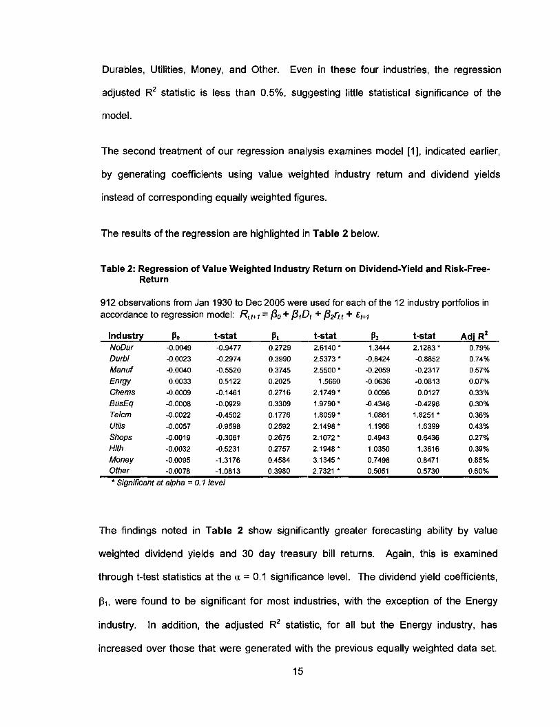
Table 2: Regression of Value Weighted Industryf Return on Dividend-Yield and Risk-Free- Return

912 observations from Jan 1930 to Dec 2005 were used for each of the 12 industry portfolios in accordance to regression model: Ri,t+l = Po + PIDt + P2rtt + Et+l

Industry 80 t-stat 81 t-stat 8 2 t-stat Adj R~ NoDur -0.0049 -0.9477 0.2729 2.6140 * 1.3444 2.1283 * 0.79%

Durbl Manuf

E W Y Chems BusEq Telcm Utils Shops Hlth Money Other -0.0078 -1.081 3 0.3980 2.7321 ' 0.5051 0.5730 0.60%

* Significant at alpha = 0.1 level

The findings noted in Table 2 show significantly greater forecasting ability by value

weighted dividend yields and 30 day treasi~ry bill returns. Again, this iis examined

through t-test statistics at the a = 0.1 significance level. The dividend yield coefficients,

p,, were found to be significant for most industries, with the exception of the Energy

industry. In addition, the adjusted R2 statistic, for all but the Energy industry, has

increased over those that were generated wit:h the previous equally weighted data set.

However, the treasury bill return coefficients, P2, are again insignifica,nt for most

industries, with the exception of Non-Durables and Telecommunications.

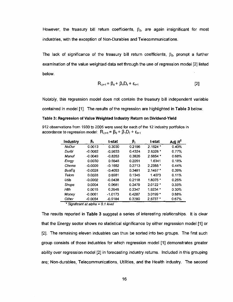
The lack of significance of the treasury bill return coefficients, P2, prompt a further

examination of the value weighted data set through the use of regression model [2] listed

below.

Notably, this regression model does not contain the treasury bill independent variable

contained in model [I]. The results of the regression are highlighted in Table 3 below.

Table 3: Regression of Value Weighted Industry Return on Dividend-Yield

912 observations from 1930 to 2005 were used for each of the 12 industry portfolios in accordance to regression model: Ri,t+l= P o + P1C)t + Et+l

Industry PO t-stat PI t-stat Adj R* - NoDur 0.001 3 0.3030 0.2196 2.1624* 0.40% Durbl Manuf

Enrgy Chems BusEq Telcm Utils Shops Hlth Money Other -0.0054 -0.9184 0.3780 2.6737 * 0.67% - * Significant at alpha = 0.1 level

The results reported in Table 3 suggest a series of interesting relationships. It is clear

that the Energy sector shows no statistical significance by either regression model [ I ] or

[2]. The remaining eleven industries can thus be sorted into two groups. The first such

group consists of those industries for which regression model [ I ] demonstrates greater

ability over regression model [2] in forecasting industry returns. Included in this grouping

are; Non-durables, Telecommunications, Utilities, and the Health industry. The second

industry grouping consists of those industries for which regression model [2]

demonstrates greater forecasting ability than regression model [ I ] and includes;

Durables, Manufacturing, Chemicals, Business Equipment, Shops, Money, and Other

industries.

As a result of the industry specific sensitivities to each regression model, it is prudent to

examine the proposed trading model over (all industries by utilizing both regression

models [ I ] and [2]. Hypothetically, one would expect to see those industries

demonstrating statistically significant relationships to also generate earnings over and

above those of the industry portfolio by employing the corresponding trading rule.

Trading Rule - Dollar Return Analysis

The results of the trading rule analysis are reported under two categories. Firstly, this

paper examines the findings of a trading rule strategy based on the earlier described

regression model [ I ] (Trading model [I]), inclusive of both the dividend yield, as well as

the monthly treasury bill rate as dependent variables. Secondly, this paper examines

the findings of a trading rule strategy based on regression model [2] (Trading model [2]),

inclusive of the dividend yield, yet excluding the monthly treasury bill rate as a

dependent variable. The trading rule analysis for both underlying regression models are

evaluated exclusively over the value weighted data set.

It would be expected that those industry portfolios demonstrating statistical significance

over the entire 1930 to 2005 examination period, would also demonstrate economic

significance in most examined sub-periods. Economic significance is defined as the

ability to produce excess returns over and above those generated by buying and holding

the industry portfolio for the duration of the examined period. Table 4 reports both the

dollar return generated by trading model [I], as well as the dollar return generated by the

industry portfolio. Specifically, reported in Table 4 is the accumulated value at the end

of each examined period of one dollar invested at the beginning of the period through

both the proposed trading rule and through investing solely in the industry portfolio.

Table 4: Dollar Return Generated by Trading Model using Dividend-Yield and Risk-Free- Return Based Forecasting vs. Dollar Return of Industry Portfolios - value weighted data

Trading Model Strategy 1940's 1950's 1960's 1970's 1980's 1990's 2000-2004 J im '40 - Dec '04

NoDur *' 2.02 2.08 2.62 3.30 5.92 3.52 1.41 1.063.24 Durbl Manuf Enrgy Chems BusEq Telcm " Utils " Shops Hlth " Money Other 1.11 3.13 1.81 3.73 4.15 4.60 1.23 553.09 Equal Weighted Portfolio 1.65 4.03 2.06 2.83 4.64 3.86 1.14 642.74

Industry Portfolio - Buy and Hold Strategy 1940's 1950's 1960's 1970's 1980's 1990's 2000-2004 J im '40 - Dec '04

NoDur 2.43 3.24 3.06 1.61 9.89 3.18 1.53 1.863.41 - - - - ~- -~ - ~ .- ~ . - ~ -

Durbl 2.66 7.00 2.07 1.62 4.35 3.31 1.19 1.069.27 Manuf E W Y Chems BusEq Telcm Utils Shops Hlth Monev 0the; 2.61 5.35 2.06 2.03 4.73 4.55 0.93 1,168.99 Equal Weighted Portfolio 2.58 5.40 2.43 1.85 5.43 4.84 1.21 1,551 .70

" lndustry portfolios found to be most significant under regression model [113

The above table contains the accumulated value at the end of each indicated period of one dollar invested at the beginning of the given period through either trading model [I], as described below, or through the industry portfolio.

A moving window of 96 historical months was used to forecast the industry return one month into the future. This process was continued every mon,th from the first January to the lasit December of the following decades: 1 %lo's, I95O1s, 1 9601s, 1 WO's, 1 9801s, 1 9901s, as well as ,for the half decade of 2000-2004, and finally for the entire period of 1940 to 2004. The forecasting model utilizes the relationship of regression model [I]: Ri,t+l = Po + PIDt + PZrf,t + &+I.

In the first month of each period the trading model invests one dollar into the portfolio indicated by the greater of the forecasted industry return or the current monthly treasury bill rate. This process is continued each subsequent month using the accumulated investment total to-date.

3 See Table 2: Regressions using Value Weighted data, model [I].

18

By examining the above table we find that over the entire period ranging from January

1940 to December 2004, the trading strategy did not produce dollar returns greater than

those of the industry portfolios even in industries that were statistically significant under

regression model [I ] . Notably, the 1970's proved to be the only decade in which the

trading model produced dollar returns greater than those of most industry portfolios, as

well as for an equally weighted portfolio of the 12 examined ind~stries.~ This outcome

can be explained by two economic factors prevalent in the 1970's. Firstly, the 1970's

were witness to historically high short term interest rates, as measured by US 30 day

treasury bill returns, averaging roughly six percent per annum for the d e ~ a d e . ~

Secondly, as indicated in Table 4 industry returns during the 1970's were at an historical

low, also averaging roughly six percent per annum. Due to the similar return~s during this

time period for both of the investment options assessed by the trading model, the trading

model portfolio return was not penalized as significantly as in other dlecades if it

incorrectly invested in the lower yielding portfolio for a given month.

The Telecommunications industry performed the best relative to its; benchmark

under the examined trading model, with $1 invested on January 1, 1930, accumulating

to almost $282 on December 31, 2004, $1 17 less than investing in the corresponding

industry portfolio for the same period. Notably, the economic performance of the trading

model on the Telecommunications industry surpassed the economic performance of the

trading model on seven other industry portfolios which possessed higher adjusted R2

statistics from the corresponding regression, analysis6 Likewise, the Non-Durables

industry which possessed the highest adjusted R2 statistic and the highest significance

The equally weighted portfolio return (EW Portfolio) is calculated as the average return over the 12 of the examined value-weighted industry portfolios. See Appendix, Table A, for the Absolute Dollar Value Return of Investing in US 30 day Treasury

Bills. 6 See Table 2: Regressions using Value Weighted data, model [l].

of both independent variables for the corresponding regression analysis, produced lower

trading model dollar returns relative to its benchmark than that of seven othler industries.

Thus, it does not appear that the level of statistical significance of the underlying

regression model corresponds directly with the level of economic significance of the

trading model. A similar examination of the industries based on the regresslion model [2]

trading model is outlined on the following page in Table 5.

Table 5: Dollar Return Generated by Trading-Model using Dividend-Yield Based Forecasting vs. Dollar Return of Industry Portfolios -value weighted data

Trading Model Strategy 1940's 1950's 1960's 1970's 1980's 1990's 2000-2004 Jian '40 - Dec '04

NoDur 2.45 2.54 3.46 2.13 7.20 1.57 1.39 721 5.6 Durbl " Manuf " Enrgy Chems ** BusEq " Telcm Utils Shops " Hlth Money " other-" 2.09 4.42 2.25 2.36 4.29 4.13 0.93 810.62 Equal Weighted Portfolio 2.1 1 4.63 2.65 1.93 4.66 3.30 1.20 743.61

Industry Portfolio - Buy and Hold Strategy 1940's 1950's 1960's 1970's 1980's 1 990's 2000-2004 Jan '40 - Dec '04

NoDur 2.43 3.24 3.06 1.61 9.89 3.18 1.53 1.863.41 Durbl Manuf Enwy Chems BusEq Telcm Utils Shops Hlth Monev 0the; 2.61 5.35 2.06 2.03 4.73 4.55 0.93 Equal Weighted Portfolio 2.58 5.40 2.43 1.85 5.43 4.84 1.21

** lndustry portfolios found to be most significant under regression model [217

The above table contains the accumulated value at the end of each indicated period of one dollar invested at the beginning of the given period through either trading model [2], as described below, or through the industry portfolio.

A moving window of 96 historical months was used to forecast the industry return one month into the future. This process was continued every month from the first January to the last December of the following decades: 1 9401s, 1 950Bs, 1 9601s, 1!3701s, 1 9801s, 1 WO's, as well as for the half decade of 2000-2004, and finally for the entire period of 1940 to 2004. The forecasting model utilizes the relationship of regression model [I]: Ri,t+l = Po + PIDt + E ~ + ~ .

In the first month of each period the trading model invests one dollar into the portfolio indicated by the greater of the forecasted industry return or the current monthly treasury bill rate. This process is continued each subsequent month using the accumulated investment total to-date.

By examining Table 5, we find that the trading model produced dollar returns in excess

of the industry portfolio return for the Business Equipment industry. Specifically, one

dollar invested through the trading model on January 1, 1940 through to December 31,

See Table 3: Regressions using Value Weighted data, model [2].

21

2004 accumulated to $27 more than if invested solely into the Business Equipment

industry portfolio over the same period. However, none of the other industries examined

produced dollar returns in excess of the corresponding industry portfolios over the 1940

to 2004 period. For this same period however, the return for an equally weighted

portfolio of all industries produced larger dollar returns through trading model [2] than

through trading model [I]. This finding in turn suggests that on average US 30 day

treasury bills provide little added economic significance to the underlying regression

relationship.

As with the results of trading model [ I ] indicated in Table 4, trading model [2]

produced dollar returns in excess of the equally weighted portfolio during the 1970's.

However unlike trading model [I], trading model [2] also produced dollar returns in

excess of the equally weighted portfolio during the 1960's. Again, this result is likely due

to the fact that as in the 1970's, the 1960's experienced a narrowing between the

difference of industry portfolio returns and US 30 day treasury bill returns over historical

norms8.

It is important to note that those industries which were found to have the greatest

statistical significance through regression model [2]: Money, Durables, Manufacturing,

and Other; were found in Table 5 to have the loth, 4th, 8th, and 5th greatest excess

returns in comparison to the industry portfolio respectively. This observation again

suggests that the economic and statistical significance of the underlying regression

relationships do not coincide with one another,.

8 See Appendix, Table A, for the Absolute Dollar Value Return of Investing in US 30 day Treasury Bills.

Trading Rule - Sharpe Ratio Analysis

Returns in excess of those generated from investing in the industry portfcdio were not

generated by either trading model [ I ] or [2] when examined on a risk un-adjiusted basis.

However, it is possible that each trading model possesses higher return per unit of risk

exposure than that of simply investing in the industry portfolio. To examine if this is

indeed true, a series of Sharpe Ratios have been calculated over both the trading model

returns and the industry portfolio returns for each examined industry and time period.'

The Sharpe Ratios can be interpreted for each portfolio over an examined period as its

return per unit of risk exposure.

Our analysis of return per unit risk begins by examining the Sharpe Ratios generated

through trading model [I]. The results of this examination are indicated in Table 6 on

the following page along with the Sharpe Ratios generated by the industry portfolios.

' Sharpe Ratio = (portfolio return - risk free return)/(portfolio standard deviation)

23

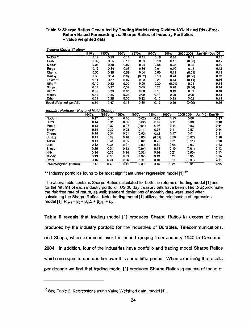
Table 6: Sharpe Ratios Generated by Trading Model using Dividend-Yield and Risk-Free- Return Based Forecasting vs. Sharpe Ratios of Industry Portfolios - value weighted data

Trading Model Strategy 1940's 1950's 1960's 1970's 1980's 1990's 2000-2004 J i m '40 - Dee '04

NoDur 0.14 0.29 0.13 0.1 1 0.18 0.18 0.09 0.15 Durbl (0.02) 0.35 0.18 0.09 0.13 0.15 (0.00) 0.12 Manuf 0.01 0.38 0.07 0.09 0.08 0.08 0.02 0.10 E W Y 0.12 0.34 0.06 0.16 0.01 0.10 0.03 0.12 Chems 0.05 0.35 0.03 0.04 0.05 0.19 (0.01) 0.11 BusEq 0.06 0.34 0.09 (0.02) 0.13 0.24 (0.08) 0.09 Telcm 0.1 1 0.37 0.07 0.08 0.21 0.14 (0.1 1) 0.1 1 Utils 0.10 0.22 0.09 0.09 0.20 (0.01) 0.08 0.11 Shops 0.18 0.27 0.07 0.09 0.23 0.26 (0.04) 0.14 Hlth " 0.09 0.23 0.05 0.00 0.13 0.19 0.01 0.10 Money 0.12 0.26 0.08 0.09 0.16 0.20 0.06 0.14 Other 0.01 0.25 0.05 0.12 0.10 0.23 0.02 0.1 1 Equal Weighted portfolio 0.10 0.47 0.11 0.10 0.17 0.26 (0.00) 0.16

Industry Portfolio - Buy and Hold Strategy 1940's 1950's 1960's 1970's 1980's 1990's 2000-2004 Jan '40 - Dec '04

NoDur 0.17 0.35 0.16 10.021 0.25 0.13 0.06 0.15 Durbl Manuf Enrgy Chems BusEq Telcm Utils Shops Hnh Monev 0the; 0.15 0.31 0.06 '0.01' 0.10 0.18 (0.03) 0.11 Equal Weighted portfolio 0.17 0.43 0.1 1 0.00 0.15 0.25 0.01 0.15

** lndustry portfolios found to be most significant under regression model [l].1•‹

The above table contains Sharpe Ratios calculated for both the returns of trading mcldel [ I ] and for the returns of each industry portfolio. US 30 day treasury bills have been used to approximate the risk free rate of return, as well; standard deviations of monthly data were used when calculating the Sharpe Ratios. Note, trading model [ I ] utilizes the relationship of regression model [I]: Ri,t+l = Po + PlDt + Pnrr,t + Et+l

Table 6 reveals that trading model [ I ] produces Sharpe Ratios in excess of those

produced by the industry portfolio for the industries of Durables, Telecommunications,

and Shops; when examined over the period ranging from January 1940 to December

2004. In addition, four of the industries have portfolio and trading model Sharpe Ratios

which are equal to one another over this same time period. When examining the results

per decade we find that trading model [ I ] produces Sharpe Ratios in excess of those of

10 See Table 2: Regressions using Value Weighted data, model [I].

the industry portfolio in the 1 9 5 0 ' ~ ~ 1970's, 19803, and 1990's. Therefore, it appears

that trading model [ I ] adds economic value over holding the industry portfolio by

increasing return per unit of risk exposure. However, industries which appear to

demonstrate greater return per unit of risk exposure through trading model [ I ] are not

necessarily those industries that had the hiighest statistical significance through the

same underlying regression model." Therefore, the risk reduction benefits of employing

trading model [ I ] may be the result of chance and are not necessarily due to any

enhanced predictive ability resulting from the regression relationship.

As with trading model [I], trading model [2] has also been examined in a similar manner

on a return per unit of risk basis. The results of this examination are indicated in Table 7

on the following page.

'' See Table 2: Regressions using Value Weighted data, model [I].

25

Table 7: Sharpe Ratios Generated by Trading Model using Dividend-Yield Based Forecasting vs. Sharpe Ratios of Industry Portfolios -value weighted1 data

Trading Model Strategy 1940's 1950's 1960's 1 970's 1980's 1990's 2000-2004 Jan '40 - Dec '04

NoDur 0.18 0.28 0.20 0.03 0.21 (0.01) 0.05 0.13 Durbl " Manuf " Enrgy Chems " BusEq " Telcm Utils Shops " Hlth Money " other-" 0.12 0.28 0.10 0.04 0.11 0.21 (0.03) 0.1 1 Equal Weighted portfolio 0.15 0.40 0.17 0.01 0.18 0.21 0.01 0.15

Industry Portfolio - Buy and Hold Strategy 1940's 1950's 1960's 1970's 1980's 1990's 2000-2004 Jan YO - Dec '04

NoDur 0.17 0.35 0.16 (0.02) 0.25 0.13 0.06 0.15 Durbl 0.14 0.31 0.06 (0.02j 0.09 0.11 0.00 Manuf 0.14 0.37 0.07 (0.01) 0.08 0.14 0.03 E W Y 0.19 0.30 0.08 0.1 1 0.07 0.11 0.07 Chems 0.14 0.31 0.01 (0.00) 0.12 0.17 0.01 BusEq 0.1 1 0.39 0.16 (0.05) (0.01) 0.28 (0.07) Telcm 0.1 1 0.41 0.05 0.02 0.25 0.21 (0.11) Utils 0.12 0.36 0.07 0.00 0.19 0.08 0.06 Shops 0.20 0.34 0.13 (0.04) 0.14 0.19 (0.01) Hlth 0.14 0.30 0.14 (0.02) 0.14 0.21 (0.00) Money 0.19 0.33 0.09 (0.02) 0.13 0.20 0.05 Other 0.15 0.31 0.06 0.01 0.10 0.18 (0.03) Equal Weighted portfolio 0.17 0.43 0.11 0.00 0.15 0.25 0.01

** lndustry portfolios found to be most significant under regression model [2]12

The above table contains Sharpe Ratios calculated for both the returns of trading model [2] and for the returns of each industry portfolio. US 30 day treasury bills have been used to approximate the risk free rate of return, as well; standard deviations of monthly data were used when calculating the Sharpe Ratios. Note, trading model [2] utilizes the relationship of regression model [2]: Ri,t+l = Po + PlDt + Et+l

The findings contained within Table 7 demonstrate that over the period ranging from

January 1940 to December 2004, trading model [2] produces Sharpe Ratios in excess of

those of the industry portfolio for the industries of Durables, Business Equipment, and

Shops. In addition, three of the industries have portfolio and trading model Sharpe

Ratios which are equal to one another. When examining the results per deciade we find

that trading model [2] produces greater Sharpe Ratios than the industry portfolio from

the 1960's through to the 1980's. Despite this;, the benefits on a risk adjusted basis of

12 See Table 3: Regressions using Value Weighted data, model [2].

26

employing trading model [2] do not appear to be as significant as those indicated in

Table 6, when employing trading model [I].

Again it appears that the industries which demonstrated enhanced risk adjusted

returns through the employment of trading model [2] were not necessarily those

industries which had the highest statistical significance from the underlying regression

model.13 Thus, little compelling evidence exists to suggest that the benefits of either

trading model, as examined on a risk adjusted basis, has resulted from the significance

of the underlying regression model.

l3 See Table 3: Regressions using Value Weighted data, model [2].

27

Summary and Conclusions

Numerous studies have been conducted for the purpose of examining the return

forecasting ability of dividend yields. Such studies have employed a variety of statistical

methodologies, yet, there has been no decisive conclusion as to whether or not any

forecasting ability of dividend yields exists. In addition, there has not been any decisive

conclusion as to which testing methodology is most appropriate to examine such a

relationship.

The analysis of Fama and French [I9881 is frequently cited by literature examining

dividend-yield based forecasting. Although the conclusions from the afo~rementioned

paper were not always supported by the body of literature that followed, there is also a

lack of significant evidence to completely dismiss the paper's findi~ngs or the

methodology that Fama and French 11 9881 proposed. Thus, the analysis presented here

borrows from the Fama and French examination by employing a similar ordinary-least-

squares (OLS) regression model to forecast future returns from historical dividend yields.

Unique to this paper are the following: first, an independent variable consisting of a risk

free rate of return, 30 day US treasury bills, is added to the regression model in an

attempt to enhance the forecasting ability of the dividend yields; second, the statistical

significance of the regression model is tested over both value and equally weighted

return and dividend yield data; third, the regression model is analyzed over 12 unique

dis-aggregated industry portfolio returns, however, the dividend yield independent

variable remains aggregated at the market level; and finally, an economic significance

test in the form of a trading model is tested against the returns of the industry portfolios

on both an absolute and risk adjusted basis.

The findings here suggest that US 30 day treasury bills do little to enhance the predictive

ability of dividend yields in forecasting future industry returns. However, the returns for

the industries of Telecommunications, Non-Durables, Utilities, and Health were better

forecasted by the regression model containing US 30 day treasury bills. Likewise,

dividend yields were found to be far more significant when used to forecast value

weighted returns over that of equally weighted returns. The statistical significance of all

employed regressions remained weak, however, with the regression models in any given

industry explaining less than 0.9% of the observed variability in industry returns, as

measured by the adjusted-R' statistic.

The regression relationships that were found to be statistically significant were then used

to formulate trading strategies in order to test, their economic significance. A series of

time periods were used to examine if a diviidend yield based trading strategy could

consistently produce excess returns on an absolute and risk adjusted basis over that of

the corresponding industry portfolio. Although the findings of our examination on a risk-

adjusted basis were promising, no conclusive evidence was found to suggest that the

underlying regression relationships was the cause of any observedl economic

significance.

The analysis presented here did not find ;any outstanding statistical or economic

significance from employing dividend yields to forecast disaggregated industry returns,

however, further examination is encouraged. The following adjustments may prove to

enhance the explanatory power of dividend yields within industry data: first, consistent

with much of the prevailing literature, the ability of dividend yields to forecast returns

increases with an increase in return horizon, therefore, examining the relationships

presented in this paper by substituting monthly data with either quarterly, semi-annual,

or annual data may uncover more significant results; likewise, utilizing mulltiple lagged

dividend yield variables may enhance the robustness of the regression ~rnodels; and

finally, it would be prudent for future examinations to test and, if necessary, control for

the presence of heteroscedasticity and autocorrelation which may be present.

Appendix

Table A: Absolute Dollar Value Return of Investing in US 30 day Treasury Bills.

1940's 1950's 1960's 1970's 1980's 1990's 2000-2004 Jan '40 - Dec '04 Risk free rate 1.04 1.20 1.46 1.84 2.34 1.62 1.14 14.65

At the beginning of each period one dollar is invested into the US 30 day Treasury Bill rate of

return (risk free rate) and accumulated to the end of the last month in the given period. The final

accumulated value of the initial investment is displayed above.

Reference List

Black, Fischer. and Scholes, Myron. (1 974), "The Effects of Dividends Yield and Dividend Policy on Common Stock Prices and Returns" Journal of Financial Economics, 1 , 1 -22.

Campbell, John Y., and Robert J. Shiller. (1988b), "The dividend-price ratio and expectations of future dividends and discount factors." Review of Financial Studies, 1, 195-228.

Fama, Eugene F., and Kenneth R. French. (1988) "Dividend Yields and Expected Stock Returns." Journal of Financial Economics, 22, 3-25.

Fama, Eugene F., and Kenneth R. French. (1988b) "Permanent and Temporary Components of Stock Prices" Journal of Political Economy, 96-2, 246-273.

Goetzmann, W., and P. Jorion. (1 995) "A Longer Look at Dividend Yields." Jcwrnal of Business, vol. 68, no. 4 (October):483-508.

Harris, Richard DF. and Sanchez-Valle Rene. (2000) "The Information Content of Lagged Equity and Bond Yields" Economics Letters, 68, 179-1 84.

Hodrick, Robert J. (1 992) "Dividend Yields and Expected Stock Returns: Alternative Procedures for Inference and Measurement." Review of Financial Studies, 5, 357-386.

Keim, Donald B. (1 985) "Dividend Yields and S,tock Returns - Implications of Abnormal January Returns" Journal of Financial Economics, 14, 473-489.

Kothari, SP., and Shanken, Jay. (1992) "Stock return variation and expected dividends" Journal of Financial Economics, 31 , 177-21 0.

Kothari, SP., and Shanken, Jay. (1997) "Book-to-Market, Dividend Yield, and Expected Market Returns: A time-series analysis" Journal of Financial economic:^, 44, 169- 203.

Purdy, Daryl. (2004) "A Dividend Yield-based Trading Rule with Industry Data!" Simon Fraser University - GA WM MBA Final Project.

Schwert, G. William. "Anomalies and Market Efficiency. (2003)"ln George M. Constantinides, Milton Harris and Rene Stultz, editors: Handbook in the Economics of Finance, Amsterdam: Elsevier Science B.V., 939-972.

Wilkie, A David. (1 993) "Can Dividend Yields Predict Share Price Changes?" Proceedings of the 3rd AFlR Colloquium, Vol 1, 335-347.

Wolf, Michael (2000) "Stock Returns and Dividend Yields Revisited: A New Way to Look at an Old Problem." Journal of Business & Economic Statistics, VOI 18, NO 1, 18-31