THE FLORIDA STATE UNIVERSITY

COLLEGE OF ARTS AND SCIENCES

PRECOMPUTED GLOBAL ILLUMINATION OF ISOSURFACES

By

KEVIN M. BEASON

A thesis submitted to theDepartment of Computer Science

in partial fulfillment of therequirements for the degree of

Master of Science

Degree Awarded:Summer Semester, 2005

The members of the Committee approve the thesis of Kevin M. Beason defended on July 26th,

2005.

David C. BanksProfessor Directing thesis

Mark SussmanOutside Committee Member

Xiuwen LiuCommittee Member

The Office of Graduate Studies has verified and approved the above named committee members.

ii

To Mom and Dad. . .

iii

ACKNOWLEDGEMENTS

Thank you very much to my advisor, David Banks, who on countless occasions went above

and beyond the call of duty to assist me in a great number of ways, including everything from

teaching, advising, pushing for my readmittance, years of funding and conference sending, to

publishing, all in the effort to provide me with a quality education. Thank you to my committee,

Mark Sussman and Xiuwen Liu, and to the many other people at FSU who assisted me along the

way, including everyone at the Vis Lab, including Josh Grant, Brad Futch, Hui Song, Wilfredo

Blanco, Chris Baker, Yoshihito Yagi, Chuck Mason, Neil Druckmann, Michael Connor, Theresa

Chen, and Kevin Kurtz. A special thanks to Mickey Boyd for his encouragement, support, and

advice. Thank you to Kayne Smith and Chris Baker for their excellent proof reading. I would

also like to thank David Gaitros, Joseph Travis, Dana Lutton, the SCS administrative staff, and

the SCS systems staff. Thank you to the scientists who provided datasets and feedback: M. Y.

Hussaini, Kayne Smith, Jorge Piekarewicz, Debra Fadool, and Wilfredo Blanco. Also, thanks to

Mike Cammarano, Steven Parker, and Henrik Jensen for heir helpful correspondences. Thank you

to FSU’s Master Craftsman Program for the bump box sculpture and light guide. Thank you to

all my friends for their support and understanding, including Matt Scragg, Mike Scragg, Melissa

Kryder, Silvana Perolini, and many other people that helped me along the way. Most importantly,

thank you to my Mom and Dad, for their infinite support and love, without which none of this

would have been possible. Also thank you to my loving sister, Laura, whom I wish the best of luck

in her upcoming schooling.

This research was supported by the SCS Visualization Laboratory and by NSF Grant #0083898.

iv

TABLE OF CONTENTS

List of Tables . . . . . . . . . . . . . . . . . . . . . . . . . . . . . . . . . . . . . . . . vi

List of Figures . . . . . . . . . . . . . . . . . . . . . . . . . . . . . . . . . . . . . . . vii

Abstract . . . . . . . . . . . . . . . . . . . . . . . . . . . . . . . . . . . . . . . . . . . viii

1. INTRODUCTION . . . . . . . . . . . . . . . . . . . . . . . . . . . . . . . . . . . 11.1 Problem description . . . . . . . . . . . . . . . . . . . . . . . . . . . . . . . 11.2 Novelty . . . . . . . . . . . . . . . . . . . . . . . . . . . . . . . . . . . . . . 31.3 Solving Light Transport . . . . . . . . . . . . . . . . . . . . . . . . . . . . . 41.4 Level Sets . . . . . . . . . . . . . . . . . . . . . . . . . . . . . . . . . . . . . 141.5 Flattened light . . . . . . . . . . . . . . . . . . . . . . . . . . . . . . . . . . 181.6 Related work . . . . . . . . . . . . . . . . . . . . . . . . . . . . . . . . . . . 191.7 Organization . . . . . . . . . . . . . . . . . . . . . . . . . . . . . . . . . . . 19

2. Using the Bump Box as a Reference Dataset . . . . . . . . . . . . . . . . . . . . . 212.1 Bump box . . . . . . . . . . . . . . . . . . . . . . . . . . . . . . . . . . . . . 22

3. ILLUMINATING A HEIGHTFIELD SURFACE . . . . . . . . . . . . . . . . . . . 253.1 Ordinary illumination . . . . . . . . . . . . . . . . . . . . . . . . . . . . . . 263.2 Flattened light . . . . . . . . . . . . . . . . . . . . . . . . . . . . . . . . . . 283.3 Flattened radiance for h : R

2 → R . . . . . . . . . . . . . . . . . . . . . . . . 293.4 Texture generation . . . . . . . . . . . . . . . . . . . . . . . . . . . . . . . . 403.5 Results . . . . . . . . . . . . . . . . . . . . . . . . . . . . . . . . . . . . . . 473.6 Physical bump box . . . . . . . . . . . . . . . . . . . . . . . . . . . . . . . . 50

4. ILLUMINATING A HEIGHTFIELD VOLUME . . . . . . . . . . . . . . . . . . . 534.1 Ordinary illumination . . . . . . . . . . . . . . . . . . . . . . . . . . . . . . 534.2 Flattened light . . . . . . . . . . . . . . . . . . . . . . . . . . . . . . . . . . 534.3 Ray tracing a 4D graph . . . . . . . . . . . . . . . . . . . . . . . . . . . . . . 554.4 Texture generation . . . . . . . . . . . . . . . . . . . . . . . . . . . . . . . . 674.5 Sampling techniques . . . . . . . . . . . . . . . . . . . . . . . . . . . . . . . 684.6 Results . . . . . . . . . . . . . . . . . . . . . . . . . . . . . . . . . . . . . . 704.7 Uniform sampling optimizations . . . . . . . . . . . . . . . . . . . . . . . . . 72

5. RESULTS ON SCIENTIFIC DATA . . . . . . . . . . . . . . . . . . . . . . . . . . 76

v

5.1 Images . . . . . . . . . . . . . . . . . . . . . . . . . . . . . . . . . . . . . . 765.2 Timings . . . . . . . . . . . . . . . . . . . . . . . . . . . . . . . . . . . . . . 835.3 Incorporating into a commercial software . . . . . . . . . . . . . . . . . . . . 855.4 Summary . . . . . . . . . . . . . . . . . . . . . . . . . . . . . . . . . . . . . 865.5 Conclusion . . . . . . . . . . . . . . . . . . . . . . . . . . . . . . . . . . . . 86

APPENDICES . . . . . . . . . . . . . . . . . . . . . . . . . . . . . . . . . . . . . . . 88

A. Ray Isosurface Intersection for A Trilinear Cell . . . . . . . . . . . . . . . . . . . . 88

REFERENCES . . . . . . . . . . . . . . . . . . . . . . . . . . . . . . . . . . . . . . . 92

BIOGRAPHICAL SKETCH . . . . . . . . . . . . . . . . . . . . . . . . . . . . . . . . 96

vi

LIST OF TABLES

2.1 Parameters for the 2D and 3D “bump box” scalar function in Equation 2.1. . . . . . 24

3.1 Root mean square (RMS) percent error of textures for the bump box scene createdby taking 20,000 samples with three sampling techniques. Textures were comparedagainst a reference texture created by using 107 regularly spaced samples. Thesampling technique with the lowest error is uniform sampling, with a RMS percenterror in pixel color of 2.16%. . . . . . . . . . . . . . . . . . . . . . . . . . . . . 50

4.1 Psuedocode for augmented ray data structure. . . . . . . . . . . . . . . . . . . . . 57

4.2 Average RMS percent error for the vertices of an isosurface rendered with height-field rendering, for three sampling strategies used to create the texture. Errorsare computed using Equation 4.11 in relation to a reference isosurface that wasdirectly rendered with photon mapping. Table shows the errors for taking 106 and107 samples using the three strategies. . . . . . . . . . . . . . . . . . . . . . . . . 72

vii

LIST OF FIGURES

1.1 Example isosurfaces. (a) Temporal evolution of turbulent jet concentration isosur-face [1] (b) iso-temperature surface calculated in a tissue volume with a number ofthermal significant blood vessels [2] (c) temperature isosurface built from satellitedata [3] (d) thermal plumes [4] (e) isosurface of density map for Bluetongue viruscapsid protein [5] . . . . . . . . . . . . . . . . . . . . . . . . . . . . . . . . . . . 1

1.2 Example datasets, shown as isosurfaces from functions of the form h : R3 → R.

(a) A superposition of five Gaussian-like density functions (b) An MRI scan ofa human brain from McGill University (c) Water density in a simulation of LaserAssisted Particle Removal (LAPR) (d) Confocal microscope scan of a living mouseneuron (e) Nucleonic densities from a simulation of the crust of a neutron star . . . 2

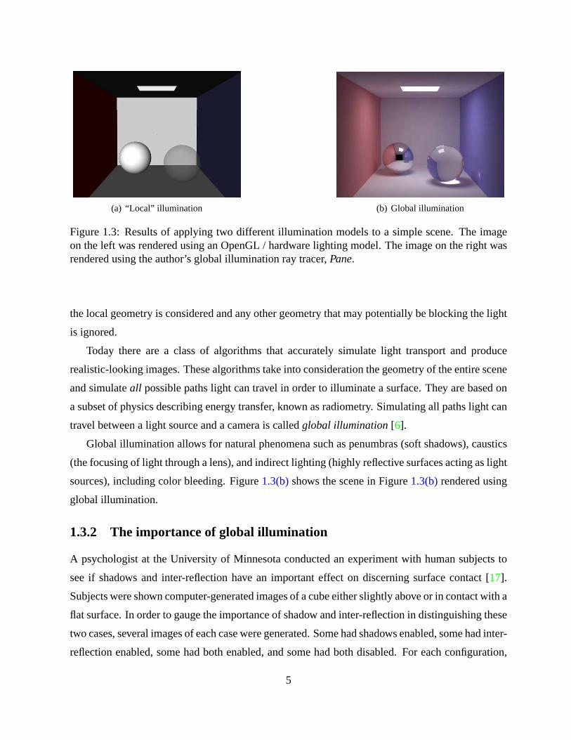
1.3 Results of applying two different illumination models to a simple scene. The imageon the left was rendered using an OpenGL / hardware lighting model. The imageon the right was rendered using the author’s global illumination ray tracer, Pane. . 5

1.4 Example benefit of global illumination. In the top row the two cylinders are farapart. In the bottom row they are close. Viewed from above (a) it is difficult todiscern the difference using local illumination (OpenGL). With global illumination(b) the shadow and inter-reflection present in the bottom scene provide naturaldistinguishing cues. A side view (c) further illustrates the difference between thetwo scenes. . . . . . . . . . . . . . . . . . . . . . . . . . . . . . . . . . . . . . . 6

1.5 Diagram of components of the Rendering Equation (Equation 1.1). Incidentradiant flux from the luminaire strikes a surface in the neighborhood dA of point~x. The incident radiance arrives from direction Li and subtends a solid angle dω ofthe hemisphere Ω. . . . . . . . . . . . . . . . . . . . . . . . . . . . . . . . . . . 8

1.6 (a) In ray tracing an image, an imaginary image plane is positioned in front of thescene camera. For each pixel in the image plane, a ray is shot from the camerathrough the pixel. At the point of intersection of the ray with the scene, a color iscomputed and this color is stored in the image at the corresponding pixel. (b) Forray tracing a scene mesh, a ray is shot at each vertex, the color is computed, andthen the color is stored at the vertex. These colors are then used the next time thescene is viewed. . . . . . . . . . . . . . . . . . . . . . . . . . . . . . . . . . . . . 9

viii

1.7 First pass of the photon mapping algorithm. Photons are fired from the light E intothe scene using ray tracing. A photon is stored where a ray intersects the scene.Some intersections spawn a refl ected ray, which may intersect the scene at a newpoint. (Redrawn from Figure 9.2 of of [6]) . . . . . . . . . . . . . . . . . . . . . 10

1.8 The refl ected radiance estimate is Lr = ∑ fr(~ω, ~ωp′)Φp

∆A , where fr(~ω, ~ωp′) is the

BRDF, Φp is the power of photon p at distance dp, and ∆A is the area of a circlewith radius max(dp) [6]. . . . . . . . . . . . . . . . . . . . . . . . . . . . . . . . 11

1.9 A simple box scene rendered using the photon map and the refl ected radianceestimate (Equation 1.4). The image took 8 seconds to render on a Dual 3.0 GHzPC. . . . . . . . . . . . . . . . . . . . . . . . . . . . . . . . . . . . . . . . . . . 12

1.10 The pattern of light on the table is a caustic created by a metal ring. This iscomputed using a special photon map. The image took 7 minutes to render ona dual 3.0 GHz PC using the author’s implementation of photon mapping. . . . . . 13

1.11 Inter-refl ection is computed in the second pass of the photon mapping algorithm.This component of Equation 1.5 accounts for the refl ection of incoming light thathas already been diffusely refl ected at least once. Monte Carlo path tracing is usedto send rays in random directions and “gather” the incoming indirect radiance.This radiance is computed at the intersection of the ray with the scene using thephoton map radiance estimate (Equation 1.4). By using a fast density estimation tocompute the radiance instead of recursing, the scene is rendered much faster. Still,this component, the “final gather,” remains the most costly to compute. (Redrawnfrom Figure 9.7 of [6]) . . . . . . . . . . . . . . . . . . . . . . . . . . . . . . . . 14

1.12 Example scientific datasets. (a) Ship wake from a computational fl uid dynamicssimulation (b) Slice of a MRI scan of a human brain (c) Maximum LikelihoodEstimation for angles of three incoming signals. . . . . . . . . . . . . . . . . . . 15

1.13 Example volume dataset. Left: slices from the volume. Right: volume renderingof the dataset created by my volume renderer. . . . . . . . . . . . . . . . . . . . . 15

1.14 (a) A single grid cell (b) All possible triangulation cases in “Marching Cubes”(MC) (c) isosurface of the bunny dataset, visualized by amira. . . . . . . . . . . . 16

1.15 A cube is split into six tetrahedra. Each tetrahedron has only three cases fortriangulation, which are shown. . . . . . . . . . . . . . . . . . . . . . . . . . . . . 17

1.16 (a) Flatland test scene: all edges are refl ective except light source BC, and anglededge, which is black. The angled obstacle causes a sharp penumbra at p and agradual one at q. (b) Radiosity as a functino of arc length along the non-blackedges of test scene. Note the sharp shadow edge at p and the gradual one at q.(Reproduced from [7]) . . . . . . . . . . . . . . . . . . . . . . . . . . . . . . . . 18

2.1 Graph of an example 2D heightfield h : Rn → R, for n = 2. The graph exists as a

surface in Rn+1. . . . . . . . . . . . . . . . . . . . . . . . . . . . . . . . . . . . 21

ix

2.2 Graph and level set of an example 2D heightfield h : Rn → R, with n = 2. The

plane Dc projecting to c in the range R contains Lc which projects to the level setLc in the domain D . . . . . . . . . . . . . . . . . . . . . . . . . . . . . . . . . . 22

2.3 An example 2D heightfield h : R2 →R. (a) The graph of the heightfield (b) Several

isolines from the heightfield (c) Overhead view of the graph placed in a box scenewith a light, forming the “ bump box” . (d) Side view of the “ bump box” . . . . . . 23

2.4 (a) Volume rendering of an example 3D heightfield h : R3 → R (b-e) Isosurfaces

of the 3D heightfield in the 3D “ bump box” test scene, for isovalues 10, 50, 100,and 150, respectively . . . . . . . . . . . . . . . . . . . . . . . . . . . . . . . . . 23

3.1 One approach to illuminating a 2D scene is to turn extrude it into a 3D scene. Left:An isoline with three “ walls” and a light. Right: The same scene extruded alongthe orthogonal direction. . . . . . . . . . . . . . . . . . . . . . . . . . . . . . . . 26

3.2 Graph of heightfield h : R2 → R illuminated using ordinary 3-dimensional light

transport. (a) Emission and refl ection occur in three dimensions (b) Resultantilluminated graph. . . . . . . . . . . . . . . . . . . . . . . . . . . . . . . . . . . 27

3.3 The surface can also be illuminated with “ fl attened” light transport. In fl attenedlight transport, emission and refl ection occur only within a 2D leaf. (a) Emissionand refl ection occur in two dimensions. (b) Resultant illuminated graph. . . . . . . 27

3.4 Light should not fl ow from one layer Dc to another layer Dc′ , for c 6= c′. . . . . . . 28

3.5 (a) The emittance distribution E : S2 → R

1 for 3D light transport is a hemisphere.(b) The emittance distribution E[ : S

1 → R1 for 3D fl attened light transport is a

hemicircle. . . . . . . . . . . . . . . . . . . . . . . . . . . . . . . . . . . . . . . 30

3.6 Flattened radiance is the radiant fl ux per unit angle per unit projected length, whered~θ is the differential angle in direction ~θ , dΛ is the differential length, and ~N[ isthe segment normal. . . . . . . . . . . . . . . . . . . . . . . . . . . . . . . . . . 31

3.7 (a) A polygonal luminaire (b) In 3D the emitted fl ux of the luminaire is just the totalfl ux Φ, which is the volume of the area A times the area fl ux density E = Φ/A. (c)In 2D the emitted fl ux of a segment of length Λ, a cross section of the luminaire,is the area Φs = ΛE = Φ/H of the cross section of the fl ux volume V = AE = Φalong the segment. (d) Φs = Φ/H generalizes to Φs = dΦ/dH, where dΦ/dH isthe ratio of the differential fl ux volume dΦ to the differential height dH. This isuseful for when the area fl ux density is known but the length fl ux density is sought. 34

3.8 Refl ectance should be about the projected normal, projected to the plane ofincidence, Dc. . . . . . . . . . . . . . . . . . . . . . . . . . . . . . . . . . . . . 36

3.9 The radiance estimate in 3 dimensions is Lr = ∑ fr(~ω, ~ωp′)Φp/dA, where fr(~ω, ~ωp

′)is the BRDF, Φp is the power of photon p at distance dp, and dA is the area of acircle with radius max(dp) [6]. . . . . . . . . . . . . . . . . . . . . . . . . . . . 38

x

3.10 The radiance estimate in 2 dimensions is Lr = ∑ fr(~θ , ~θp′)Φp/(dHdΛ), where

fr(~θ , ~θp′) is the BRDF, Φp is the power of photon p at distance dp, and dHdΛ

is the projected area dA of a circle with radius max(dp). . . . . . . . . . . . . . . 38

3.11 Chart showing the 15 cases for Marching Squares [8]. A case exists for eachcombination of the cell’s corners being greater than (white) or less than (black)the isovalue. If an edge straddles the isovalue (meaning one corner is higher whileanother is lower), an intersection exists and is connected to other intersectionsaccording to the chart. Red lines indicate a possible ambiguity in connectivity (inthese cases the connections chosen are arbitrary). . . . . . . . . . . . . . . . . . . 40

3.12 Two competing approaches to illuminating the graph of a heightfield function: (a)Sampling level sets and illuminating them in the domain D . (b) Sampling positionson the graph and computing the illumination in D ×R using fl attened illumination. 42

3.13 Weighting functions for scattered data interpolation, as a function of distance dfrom a texture voxel. (a) Inverse power function, wi(x,y) = d−5. This function hasinfinite support and is shown with a log scale for the vertical axis. (b) Tent filterfunction, wi(x,y) = 1−d/R, where R is the radius of the filter. This function has asupport of 2R. . . . . . . . . . . . . . . . . . . . . . . . . . . . . . . . . . . . . 44

3.14 Interpolation of 200 samples into texture using weight function wi(x,y) = d−q,where d is the distance between (x,y) and sample point (xi,yi), for varying valuesof q. Here dmax = ∞ so all points were considered. . . . . . . . . . . . . . . . . . 45

3.15 Interpolation of 20,000 samples using Equation 3.11 into a texture using sampleweighting function wi(x,y) = d−5 for samples with distance d < dmax for varyingvalues of dmax. . . . . . . . . . . . . . . . . . . . . . . . . . . . . . . . . . . . . 45

3.16 (a) A surface rendered with ordinary light transport using only the direct lightingcomponent. (b) A surface rendered with fl attened light transport appears toobright by a factor of π

2 due to a different normalization constant. (c) The resultof multiplying the final radiance by the inverse fraction π

2 ≈ .6366 more closelymatches the appearance of the surface rendered using ordinary light transport. . . . 47

3.17 (a) 20,000 samples uniformly spread throughout the graph of h(x,y). (b) Resultingtexture with dmax = 1 (c) Resulting texture with dmax = 16 (d) Colored isoline forisovalue=47. . . . . . . . . . . . . . . . . . . . . . . . . . . . . . . . . . . . . . 47

3.18 (a) 20,000 non-uniform samples located in the region contained in the letters “ B” ,“A” , “ D” . Note that the region at the bottom (near the luminaire) is unsampled,so the interpolated radiance there poorly matches Figure 3.20(a). (b) Resultingtexture with dmax = 1 (c) Resulting texture with dmax = 566 (d) Colored isoline forisovalue=47. . . . . . . . . . . . . . . . . . . . . . . . . . . . . . . . . . . . . . 48

xi

3.19 (a) 20,000 uniform samples located along 10 level sets Lc of h(x,y). (b) Resultingtexture with dmax = 1 (c) Resulting texture with dmax = 400. Notice that aliasing(seen as bands) is clearly visible. (d) Colored isoline for isovalue=47. . . . . . . . 48

3.20 Textures for 2D bump box data set. (a) Reference texture, created with 107

regularly spaced samples (b) Uniform sampling texture, created with 20,000uniformly distributed samples (c) Non-uniform sampling texture, created with20,000 non-uniform samples located in the region contained in the letters “ B” , “A” ,“ D” (d) Undersampling texture, created with 20,000 samples distributed acrosslevel sets of 10 isovalues. . . . . . . . . . . . . . . . . . . . . . . . . . . . . . . 49

3.21 The bump box illuminated by a line segment. . . . . . . . . . . . . . . . . . . . . 51

3.22 Illuminating the bump box. The upper row shows the function f : R2 →R graphed

as a height field in R3. The lower row shows the illumination grid, which is the

height field’s color as seen from overhead, projected to the domain of f . . . . . . . 52

4.1 Left: The emittance distribution E : S3 → R

1 for 4D light transport is difficult toimagine and draw. Right: The emittance distribution E[ : S

2 →R1 for 4D fl attened

light transport is just the same as in ordinary 3D light transport: a hemisphere. . . 55

4.2 Labelling of a cell. The cell’s corner are eight neighboring voxels in a rectilineargrid, a small piece of a volume heightfield h : R

3 →R. Figure reproduced from [9]Fig. 15 . . . . . . . . . . . . . . . . . . . . . . . . . . . . . . . . . . . . . . . . . 59

4.3 Top: Photons emit from a light carrying “ fl ux-height” . Bottom: (Left) The photonscollect in leaves of the graph of h. (Right) A cylindrical volume of photons,extending through both the domain and range of h, is found in order to make aradiance estimate. The fl ux-height of the photons is added and the sum is dividedby the height of the cylinder to yield the approximate fl ux. This fl ux is then dividedby the surface area of the top of the cylinder, A = πr2, to find the fl ux-area-densityE. . . . . . . . . . . . . . . . . . . . . . . . . . . . . . . . . . . . . . . . . . . . 62

4.4 The radiance estimate in four dimensions is L[r = f [

r ∑Fp/∆V , where fr is theBRDF, Fp is the fl ux-height of photon p at distance dp, and ∆V ≈ ∆A ∆h is thevolume of the region containing the photons. Shown are three possible choicesof volumes to use in an estimate. (a) uses a box region (b) uses a clipped sphere(c) uses a cylinder. My implementation uses the clipped sphere (b) for simplicitywhen doing a photon search in the photon map (a four dimensional kd-tree) [10]. . 64

4.5 Labelling of components of a clipped sphere. d is the radius of the sphere, whered =

√

∆x2 +∆y2 +∆z2 +(κ∆h)2. At height h, the radius of the lateral disc isr =

√d2 −h2. The volume of the sphere clipped at h = κhmin and h = κhmax is

∆V = π(d2κhmax − (κhmax)3

3 )−π(d2κhmin − (κhmin)3

3 ). This volume is used in thefl attened 4D photon mapping radiance estimate in Equation 4.8. . . . . . . . . . . 66

xii

4.6 Top row: (Left) 106 uniformly distributed samples of L[ on the graph of h. (Middle)Resulting texture. (Right) Textured isosurface for h = 47. Middle row: (Left)106 samples, distributed among small set of diagonal planes. (Middle) Resultingtexture. (Right) Textured isosurface. Bottom row: (Left) 106 samples, distributedacross a small set of isovalues. (Middle) Resulting texture. (Right) Texturedisosurface. . . . . . . . . . . . . . . . . . . . . . . . . . . . . . . . . . . . . . . 69

4.7 Isosurface for isovalue 47 from 3D “ bump box” data set. (a) Reference iso-surface rendered with Pane using normal 3D light transport (b) Isosurface fromtexture sampled with 106 uniformly distributed samples (c) Isosurface from texturesampled with 106 samples distributed on angular slabs at regular intervals in thedomain of the graph of h (d) Isosurface from texture sampled with 106 samplesdistributed across a small set of isovalues . . . . . . . . . . . . . . . . . . . . . . 71

4.8 Samples of the illumination on the graph of an example one-dimensional (1D)heightfield. The illumination samples are filtered into a 1D texture linear in thedomain. (a) Uniform sampling in the domain of the graph can leave relativelylarge gaps in the domain. For example, the texel for the large, front facing bump,highlighted in red, does not receive a sample. This is a bad situation since thehill is exists at many heights and is visible in a large proportion of level sets. (b)Regularly spacing the samples or using stratified (jittered) samples gives lowerdiscrepancy, guaranteeing the aforementioned texel at least one sample. (c) Takingtwice as many regular samples improves the texture quality, giving each texel twosamples. However, the large bump is still under sampled. (d) One approach isto supersample these areas more than less important areas, thus saving samples.This is achieved by performing more supersampling in regions that span a greatertotal extent in the range. Here the large forward facing bump receives four sampleswhile other regions receive only one sample, using the same number of samples asin (c). . . . . . . . . . . . . . . . . . . . . . . . . . . . . . . . . . . . . . . . . . 73

4.9 Focusing samples in regions that span a large extent of the range of the functioncan greatly improve texture quality. (a) Result of 4 million stratified, uniformlydistributed illumination samples on the neuron dataset. (b) Taking 64 millionstratified, uniformly distributed illumination samples eliminates the noise. (c)Taking just 2 million importance samples using Equation 4.12 performs as wellas well as taking 32 times as many samples (b). . . . . . . . . . . . . . . . . . . . 74

5.1 (a) Level set of the nucleons dataset for h = 39, top angle view, rendered using localillumination (OpenGL), requiring 1400 milliseconds to extract and display. (b)The same level set rendered using heightfield rendering with global illumination,requiring 1460 milliseconds to extract and display. The precomputation time forthe heightfield rendering 3D texture was 9685 seconds. . . . . . . . . . . . . . . . 77

5.2 (a) Front view of level set of nucleons dataset for h = 39, rendered with localillumination. (b) Level set rendered with heightfield rendering. . . . . . . . . . . . 77

xiii

5.3 (a) Level set for h = 24 from the nucleon level set, rendered using local illumina-tion (OpenGL), requiring XXX milliseconds to extract and display. (b) Level setfor h = 24 rendered using heightfield rendering. (c) Level set for h = 24 rendereddirectly using ordinary photon mapping, requiring 2155 seconds to render. Noticethat the heightfield-rendered and directly-rendered images are nearly identical. Theaverage RMS error for the vertex colors between the heightfield-rendered level setand the directly-rendered version is 5.61%. . . . . . . . . . . . . . . . . . . . . . 78

5.4 Level sets of the nucleon dataset for different isovalues: h = 170, h = 79, h = 39,and h = 24. Images were rendered using global illumination via heightfieldrendering, requiring 3.473 seconds per level set (average) for extraction anddisplaying. . . . . . . . . . . . . . . . . . . . . . . . . . . . . . . . . . . . . . . 78

5.5 (a) Level set of LAPR dataset for h = 112 rendered with local illumination,requiring 0.880 seconds to extract and display. (b) Same level set rendered withglobal illumination via heightfield rendering, requiring 0.920 seconds to extractand display. Heightfield rendering required 5565 seconds to precompute theillumination into a texture. . . . . . . . . . . . . . . . . . . . . . . . . . . . . . . 79

5.6 (a) Level set of LAPR dataset for h = 112 rendered with local illumination. (b)Same level set rendered with global illumination via heightfield rendering. . . . . 79

5.7 Five level sets of the LAPR dataset for isovalues h = 201, h = 166, h = 116, h = 76,and h = 52. Images were rendered using global illumination via heightfield render-ing, and took 1.065 seconds per isovalue (average) for extraction and displaying.

. . . . . . . . . . . . . . . . . . . . . . . . . . . . . . . . . . . . . . . . . . . . 80

5.8 (a) Level set of the neuron dataset for h = 150 rendered with local illumination,requiring 0.870 seconds to extract and display. (b) Same level set rendered withglobal illumination via heightfield rendering, requiring 0.880 seconds to extractand display. Heightfield rendering required 4587 seconds to precompute theillumination into a texture. . . . . . . . . . . . . . . . . . . . . . . . . . . . . . . 81

5.9 Front view of level set of neuron dataset for h = 85. (a) Rendered with localillumination. (b) Rendered with global illumination via heightfield rendering. . . . 81

5.10 Four level sets of the neuron dataset for isovalues h = 107, h = 88, h = 78, andh = 49. Images were rendered with global illumination via heightfield rendering,taking 0.838 seconds per level set (average) for extraction and displaying. . . . . . 82

5.11 Level set of the brain dataset for h = 77. (a) Rendered with local illumination,requiring 4.450 seconds to extract and display. (b) Same level set rendered withglobal illumination via heightfield rendering, requiring 4.680 seconds to extractand display. Heightfield rendering required 5452 seconds to precompute theillumination into a texture. . . . . . . . . . . . . . . . . . . . . . . . . . . . . . . 83

xiv

5.12 Top view of level set of brain dataset for h = 77. (a) Rendered with localillumination. (b) Rendered with global illumination via heightfield rendering. . . . 83

5.13 Four level sets of the brain dataset for isovalues h = 106, h = 97, h = 82, andh = 19. Images were rendered using global illumination via heightfield rendering,requiring 3.473 seconds per level set (average) for extraction and displaying. . . . 84

5.14 Timings and errors for heightfield rendering of four scientific datasets. Errorsare for a single (arbitrary) texture-mapped isosurface versus a reference directly-rendered isosurface, and were computed using Equation 4.11. . . . . . . . . . . . 85

5.15 Incorporating pre-computed global illumination into the commercial visualizationtool “ amira.” Top: Data fl ow network of amira modules. Bottom: (left) Levelset displayed with amira’s native lighting model; (right) displayed with 3D globalillumination texture. . . . . . . . . . . . . . . . . . . . . . . . . . . . . . . . . . . 86

A.1 Labelling of a cell. The cell’s corner are eight neighboring voxels in a rectilineargrid, a small piece of a volume heightfield h : R

3 →R. Figure reproduced from [9]Fig. 15 . . . . . . . . . . . . . . . . . . . . . . . . . . . . . . . . . . . . . . . . . 88

A.2 Coordinate systems use for interpolation and intersection. Figure modified (cor-rected) version from [9] Fig. 16 . . . . . . . . . . . . . . . . . . . . . . . . . . . 90

xv

ABSTRACT

Three dimensional scalar heightfields, also known as volumetric datasets, abound in science

and medicine. Viewing the isosurfaces, or level sets, is one of the two main ways to display these

datasets, the other being volume visualization. Typically the isosurfaces are rendered on a personal

computer (PC) allowing the scientist or doctor analyzing the dataset to interactively change the

isovalue, and rotate or zoom the isosurface. Unfortunately, out of necessity due to the PC’s video

card, current techniques render the isosurfaces with a basic hardware-accelerated lighting model.

This lighting model lacks important features such as shadows, and as a result the isosurfaces are

more difficult to interpret than if they had been rendered with a physically based lighting model.

My thesis is that isosurfaces can be displayed with realistic illumination at interactive

rates on a typical PC. I present a method for applying global illumination to interactively

created isosurfaces, using a physically based lighting model, with a negligible increase in the

time required to render the isosurfaces. The result is convincing shading that is easy to interpret

by the human visual system, including features such as soft shadows, inter-refl ection, caustics, and

color bleeding. This is achieved by solving the rendering equation for all isosurfaces within the

volume, storing the solutions in a 3D texture, and then texture mapping the result onto a polygonal

approximation of the isosurface. This process is called “ heightfield rendering” .

xvi

CHAPTER 1

INTRODUCTION

1.1 Problem description

“ Scientific visualization” is a practice whose origins trace to the massive datasets generated from

computational simulations (chiefl y using supercomputers at national research laboratories) of

physical phenomena. The archetypical dataset is a scalar function h : R3 → R representing, for

example, density, pressure, or temperature. As Hamming noted, “ [the] purpose of computation is

insight, not numbers” [11]. The premiere technique for displaying such a dataset is to generate its

level sets (isosurfaces) Lconst = ~p : h(~p) = const. These surfaces convey qualitative aspects of

the function to the scientific user analyzing the data. Examples are presented in Figure 1.1.

In the field of computer graphics, considerable success has been achieved in creating photo-

realistic renderings of surfaces by solving the integral equation for light transport. Such realistic

images offer important shape-from-shading cues to the human visual system. Current research

in rendering concerns producing these high quality images at interactive rates (1 Hz or faster).

(a) (b) (c) (d) (e)

Figure 1.1: Example isosurfaces. (a) Temporal evolution of turbulent jet concentration isosurface[1] (b) iso-temperature surface calculated in a tissue volume with a number of thermal significantblood vessels [2] (c) temperature isosurface built from satellite data [3] (d) thermal plumes [4] (e)isosurface of density map for Bluetongue virus capsid protein [5]

1

(a) bump box (b) Nucleons (c) LAPR (d) Neuron (e) Brain

Figure 1.2: Example datasets, shown as isosurfaces from functions of the form h : R3 → R. (a)

A superposition of five Gaussian-like density functions (b) An MRI scan of a human brain fromMcGill University (c) Water density in a simulation of Laser Assisted Particle Removal (LAPR)(d) Confocal microscope scan of a living mouse neuron (e) Nucleonic densities from a simulationof the crust of a neutron star

However, there has been no effort to date in the visualization community either to solve the

equation for light transport on isosurfaces or to make the process fast enough for the scientist

to view the illuminated isosurfaces on an ordinary desktop computer. My thesis is that both goals

can be achieved. That is, globally illuminated isosurfaces of a scalar function h : R3 → R can

be generated and displayed at interactive rates on an ordinary desktop computer equipped

with a graphics card. I demonstrate this thesis by (1) solving a modified version of the light

transport equation on the graph of h, (2) storing the solution in a three dimensional (3D) texture,

and then (3) texture mapping the result onto a polygonal approximation of the isosurface. I call

this 3-step pipeline “ heightfield rendering” .

I demonstrate heightfield rendering on actual datasets produced by scientists at Florida State

University (FSU) and McGill University [12], plus one (analytically defined) reference dataset that

I call the “ bump box.” Figure 1.2(a) shows the bump box dataset consisting of the superposition

of five 3D Gaussian-like functions with varying parameters. The second dataset, whose isosurface

is shown in Figure 1.2(b), is a density convolution of the exotic nuclear structures in the crust of

a neutron star. This dataset is from Dr. Jorge Piekarewicz in the Department of Physics at FSU

and Brad Futch in the School of Computational Science (SCS) at FSU. Next, Figure 1.2(c) shows

density data from a molecular dynamics simulation of Laser Assisted Particle Removal (LAPR),

conducted by Dr. M.Y. Hussaini and Dr. Kayne Smith in SCS at FSU. Figure 1.2(d) shows the

fourth dataset, from a confocal microscope scan of a living mouse neuron. This dataset is from

Debra Fadool in the Department of Neuroscience at FSU, and Wilfredo Blanco in SCS at FSU.

2

Lastly, Figure 1.2(e) is a Magnetic Resonance Imaging (MRI) scan of a human brain, scanned at

the McConnell Brain Imaging Center at McGill University.

1.2 Novelty

The novel contributions contained herein are as follows:

1. The thesis (from Page 2) is proved by example. (Page 86)

2. I introduce the “ bump box” as an analytically defined reference function. (Page 22)

3. I expand on the idea of storing global illumination in a texture (similar to vicinity shad-

ing [13]). (Page 67)

4. I introduce the idea of foliating the domain D of a heightfield h : Rn → R into level sets and

illuminating each level set of D . (Page 42)

5. I introduce the idea of foliating the graph of a heightfield and illuminating each raised level

set in D ×R, where R is the range of the heightfield function. (Page 41)

6. I introduce the idea of fl attened illumination of a heightfield function within D × R.

(Page 28)

7. I provide a definition of, equations for, and an implementation of fl attened emittance.

(Page 32)

8. I define, provide equations for, and implement fl attened refl ectance. (Page 36)

9. I provide a brightness correction term for fl attened 3D rendering. (Page 46)

10. I devise a 3D photon-map-based fl attened radiance estimate. (Page 38)

11. I decouple sampling the radiance of a heightfield surface from level set generation. (Page 43)

12. I compare the error of different graph sampling techniques. (Page 71)

13. I demonstrate heightfield rendering on actual datasets from medicine, astrophysics, neuro-

science, and nanochemistry. (Page 76)

3

14. I demonstrate incorporating heightfield rendering into a commercial visualization software

(amira from Template Graphics Systems). (Page 85)

15. I provide a corrected version of the algorithm by Parker et al. [9] to find a ray-isosurface

intersection for trilinear boxes. (Page 88)

1.3 Solving Light Transport

1.3.1 Introduction to global illumination

In the real world, light refl ects off surfaces onto other surfaces. If the material is transparent, such

as glass, light may transmit through the surface. The transmission and refl ection of light is called

light transport. Regions that receive less light because objects are obstructing the light source are

in shadow. If light has bounced off at least one surface before arriving at a region, the light is

called indirect light, or indirect illumination. This bouncing of light from one surface to another is

inter-reflection.

Photo-realistic means a picture looks similar to, or is indistinguishable from, an actual

photograph. Making photo-realistic images is called realistic image synthesis. Typically a scene

description is created, containing a 3-dimensional model along with the position of lights and a

camera, and given as input to a program which generates an image. The quality of the generated

image, in particular the degree of photo-realism achieved, depends on the shading algorithm the

program implements [14].

Early shading algorithms such as Phong’s [15] and Blinn’s [16] simulate local shading effects.

Local shading effects occur if the scene is composed of only the region in question and the light

source. These algorithms do not consider how the scene as a whole may refl ect or occlude the light,

because it was considered too computationally expensive to account for these large-scale complex

interactions. As a result, this simple type of illumination is known as local illumination. OpenGL

is probably the most prominent example of local illumination. OpenGL is a standard interactive

graphics library and employs a local illumination model by default.

For example, Figure 1.3(a) shows a simple scene rendered using OpenGL’s local illumination

shading. The scene appears fake because a simple local illumination computation is performed at

the corners of the scene and the colors are linearly interpolated across the surfaces. Even if the

shading is performed per-pixel, important features such as shadows will be absent because only

4

(a) “ Local” illumination (b) Global illumination

Figure 1.3: Results of applying two different illumination models to a simple scene. The imageon the left was rendered using an OpenGL / hardware lighting model. The image on the right wasrendered using the author’s global illumination ray tracer, Pane.

the local geometry is considered and any other geometry that may potentially be blocking the light

is ignored.

Today there are a class of algorithms that accurately simulate light transport and produce

realistic-looking images. These algorithms take into consideration the geometry of the entire scene

and simulate all possible paths light can travel in order to illuminate a surface. They are based on

a subset of physics describing energy transfer, known as radiometry. Simulating all paths light can

travel between a light source and a camera is called global illumination [6].

Global illumination allows for natural phenomena such as penumbras (soft shadows), caustics

(the focusing of light through a lens), and indirect lighting (highly refl ective surfaces acting as light

sources), including color bleeding. Figure 1.3(b) shows the scene in Figure 1.3(b) rendered using

global illumination.

1.3.2 The importance of global illumination

A psychologist at the University of Minnesota conducted an experiment with human subjects to

see if shadows and inter-refl ection have an important effect on discerning surface contact [17].

Subjects were shown computer-generated images of a cube either slightly above or in contact with a

fl at surface. In order to gauge the importance of shadow and inter-refl ection in distinguishing these

two cases, several images of each case were generated. Some had shadows enabled, some had inter-

refl ection enabled, some had both enabled, and some had both disabled. For each configuration,

5

(a) Local illumination (b) Global Illumination (c) Side view

Figure 1.4: Example benefit of global illumination. In the top row the two cylinders are far apart.In the bottom row they are close. Viewed from above (a) it is difficult to discern the differenceusing local illumination (OpenGL). With global illumination (b) the shadow and inter-refl ectionpresent in the bottom scene provide natural distinguishing cues. A side view (c) further illustratesthe difference between the two scenes.

the subjects were asked to decide whether or not the cube was touching the surface. The conclusion

was that shadows played a very important role in correctly determining surface contact, and

indirect illumination played an equally important role. The study found, however, that the greatest

sensitivity to surface contact was achieved when both shadows and indirect illumination were

present.

Figure 1.4 illustrates the benefit of these lighting components. The top row shows a scene

where two cylinders are very close. The bottom row shows a similar scene where they are far

apart. Viewed from above and rendered with local illumination (OpenGL), these scenes are

indistinguishable. However, when rendered using global illumination the shadows and inter-

refl ection caused by the proximity of the tubes in the top row makes the difference obvious.

6

1.3.3 Computing global illumination

Simulating light transport is a challenging task. However, techniques exist to compute it efficiently.

In image synthesis, the main goal is to find the color of each pixel in an image. The color represents

light energy hitting the eye, so the problem becomes determining what energy is coming from the

direction of each pixel.

What are the units of light energy for each pixel? The answer to this involves radiant fl ux.

Radiant flux, Φ, is the time rate of fl ow of energy, Q, contained in the photons making up the light,

and is expressed in Joules/second or Watts:

Φ =dQdt

.

The color of a pixel is determined by the radiance. Radiance is expressed in units of radiant

fl ux per unit projected area per unit solid angle, or Watts per meters squared per steradian in SI

units1, and is given by:

L(~x, ~ω) =d2Φ

dA cosθ d~ω,

where dA is the differential area receiving light from direction d~ω , and θ is the angle between ~ω

and the surface area normal.

Radiant energy is composed of photons at different wavelengths, however this explanation will

ignore any wavelength dependence. The task of global illumination algorithms is to determine the

radiance for each pixel. This value comes from the rendering equation (Equation 1.1) explained in

the next section.

The Rendering Equation

The formula for radiance from a surface was first published by Kajiya in 1986 [18]. Today

this formula is well known and understood to be the standard model for light transport between

surfaces, and is called the Rendering Equation:

L(~x, ~ω) = Le +∫

Ωfr(~ω, ~ω ′)Li(~x, ~ω

′) (~N · ~ω ′) d~ω ′ . (1.1)

1 In practice, the radiance is usually scaled by the spectral response of the human visual system, thereby turningit into luminance, and then the luminance is stored as the color of the pixel. However, this post-process is not alwaysnecessary and is ignored in this thesis.

7

Figure 1.5: Diagram of components of the Rendering Equation (Equation 1.1). Incident radiantfl ux from the luminaire strikes a surface in the neighborhood dA of point~x. The incident radiancearrives from direction Li and subtends a solid angle dω of the hemisphere Ω.

The rendering equation states that the radiance, L(~x, ~ω), coming from a surface at point ~x in

direction ~ω , is equal to the emitted radiance, Le, plus the integral (sum) of the incident radiance, Li,

over a hemisphere, Ω, scaled by a Bidirectional Refl ectance Distribution Function (BRDF) [19],

fr, and the dot product of ~ω ′ and the surface normal ~N. See Figure 1.5 for a diagram of these

components.

The rendering equation is a Fredholm integral equation of the second kind because one of the

unknowns appears outside the integral, making the equation recursive. That is, in order to calculate

the outgoing radiance, the incoming radiance must be known, which uses the same formula. I show

how to solve this equation, and thus global illumination and light transport, by using ray tracing.

Ray tracing

A ray is a parametric line specifying a position ~r given a parameter t, starting position ~o, and

direction vector ~d using the formula~r = ~o + t~d [20]. Ray tracing is the process of tracing a ray

through a scene to find the first object it intersects, and the point of intersection. Ray tracing was

introduced by Whitted in 1980 [21] in order to create an image of a scene. First a camera and

an image plane are determined, then rays are traced from the camera through pixels in the image

plane. Once the point of intersection between the ray and the scene is found, a color is computed

and stored at the corresponding pixel. The program that performs this computation is called a ray

tracer.

8

Figure 1.6: (a) In ray tracing an image, an imaginary image plane is positioned in front of thescene camera. For each pixel in the image plane, a ray is shot from the camera through the pixel.At the point of intersection of the ray with the scene, a color is computed and this color is stored inthe image at the corresponding pixel. (b) For ray tracing a scene mesh, a ray is shot at each vertex,the color is computed, and then the color is stored at the vertex. These colors are then used thenext time the scene is viewed.

It is simple to modify a ray tracer to store the computed colors at the vertices of the triangles

that make up a scene mesh rather than at the pixels the rays go through. To do this, rays are fired

at each vertex of each triangle in the scene from a small distance above the triangle and very close

to the vertex. The computed color is then stored along with the vertex in the scene description.

In Open Inventor, this is done using a per-vertex material binding. Figure 1.6 illustrates these two

methods of ray tracing.

The speed of the ray-object intersection computation is critical in solving global illumination

in a timely manner. A naive straight-forward approach of testing every n objects in a scene for

intersection with a ray has time complexity O(n) (linear). This is prohibitively expensive for

typical scenes, for which n may be several million or more. Instead, space subdivision techniques,

including uniform grids [20], BSP trees [22], hierarchical bounding volumes [23], and octrees

[24], are employed to test only those objects likely to be intersected. These intersection algorithms

typically have time complexity O(logn), a significant improvement.

Photon mapping

Photon mapping is a global illumination algorithm, developed by Henrik Wann Jensen in 1996

[25] that uses ray tracing. It belongs to a class of global illumination algorithms that perform

Bidirectional Path Tracing and, compared to other techniques, is extremely efficient.

For example, Monte Carlo path tracing (MCPT) [20], a straightforward technique to solve the

9

Figure 1.7: First pass of the photon mapping algorithm. Photons are fired from the light E into thescene using ray tracing. A photon is stored where a ray intersects the scene. Some intersectionsspawn a refl ected ray, which may intersect the scene at a new point. (Redrawn from Figure 9.2 ofof [6])

rendering equation, requires eight hours on a Dual 3.0 Gigahertz (GHz) PC to compute the image

shown in Figure 1.3(b), and the result contains noise. Photon mapping, however, renders the image

with virtually no noise in just six minutes on the same machine.

The idea of bidirectional path tracing algorithms such as photon mapping is that rays are not

only fired from the camera (as in MCPT), but are also traced from the light sources into the scene.

In photon mapping these interactions are stored as particles named photons in a data structure

called the photon map.

Photon mapping is a two-pass algorithm. In the first pass photons are emitted from the light

sources into the scene. The photons refl ect, absorb, transmit, and scatter throughout the scene just

as real photons would. See Figure 1.7. The number of photons used is user-controlled, but their

sum carries the radiant power of the light source. For example, using n photons for a light source

with power Φ, each photon p has power Φn . That is,

Φp =Φn

, p ∈ 1, ...,n . (1.2)

The photon map approximates the light power distribution in the scene. Each photon represents

a discrete amount of fl ux. The sum of the power of several photons on a small surface area patch

gives an estimate of the total fl ux arriving at that surface patch. Dividing this total fl ux by the area

10

Figure 1.8: The refl ected radiance estimate is Lr = ∑ fr(~ω, ~ωp′)Φp

∆A , where fr(~ω, ~ωp′) is the BRDF,

Φp is the power of photon p at distance dp, and ∆A is the area of a circle with radius max(dp) [6].

of the surface patch yields an estimate of the local fl ux density, or power per unit area:

E ≈n

∑p=1

Φp

∆A. (1.3)

Multiplying each photon’s power Φp by the BRDF fr(~ω, ~ωp′) yields the following estimate of

the refl ected radiance:

Lr ≈n

∑p=1

fr(~ω, ~ωp′)

Φp

∆A, (1.4)

where ∆A is a small area containing n photons, ∆Φp is the power of the pth photon, and fr is

the BRDF. See Figure 1.8 for a diagram. When added to the emitted radiance Le, Equation 1.4

provides an estimate of the total radiance leaving a point on the surface patch, approximating the

rendering equation, Equation 1.1.

Figure 1.9 shows the example scene in Figure 1.3 rendered using the photon map. The scene

is blotchy, which is typical, but this is corrected during a second pass. The second pass splits

the radiance computation into four parts and uses the power distribution approximation contained

within the photon map to create a final image. This splitting is done as follows. Incident light,

Li, is split into three components: direct illumination, Li,l , indirect illumination, Li,d , and specular

illumination, Li,c (e.g., off mirrors or glass). The BRDF, fr, is also split into two parts: a diffuse

component, fr,D, and a specular component, fr,S. The rendering equation (Equation 1.1) then

becomes:

11

Figure 1.9: A simple box scene rendered using the photon map and the refl ected radiance estimate(Equation 1.4). The image took 8 seconds to render on a Dual 3.0 GHz PC.

L(~x, ~ω) =Le +∫

Ωfr(~ω, ~ω ′)Li(~x, ~ω

′) (~N · ~ω ′) d~ω ′

=Le +∫

Ω( fr,S(~ω, ~ω ′)+ fr,D(~ω, ~ω ′)) (Li,l(~x, ~ω

′)+Li,c(~x, ~ω′)+Li,d(~x, ~ω

′)) (~N · ~ω ′) d~ω ′

=Le +∫

Ωfr,D(~ω, ~ω ′)Li,l(~x, ~ω

′) (~N · ~ω ′) d~ω ′+ (1.5a)∫

Ωfr,S(~ω, ~ω ′) (Li,l +Li,c +Li,d)(~x, ~ω

′) (~N · ~ω ′) d~ω ′+ (1.5b)∫

Ωfr,D(~ω, ~ω ′)Li,c(~x, ~ω

′) (~N · ~ω ′) d~ω ′+ (1.5c)∫

Ωfr,D(~ω, ~ω ′)Li,d(~x, ~ω

′) (~N · ~ω ′) d~ω ′. (1.5d)

Briefl y, the four integral components in Equation 1.5 are computed as follows. Equation 1.5a,

the direct lighting estimate, is computed by using Monte Carlo integration and “ shadow rays” to

test visibility of the light source [26]. In this case, the shadow rays are shot directly at the lights

rather than randomly (as in MCPT) and there is no recursion.

Equation 1.5b accounts for specular lighting, and is computed by sending a ray in the specular

direction, and where the ray intersects, recursively solving Equation 1.5. While the calculation is

recursive, for mirror-like surfaces only one recursive ray at each level of recursion is needed. This

is a great simplification over having two (or more) recursive rays, because such recursion would

result in an exponential growth in the number of rays for which Equation 1.5 must be solved.

Equation 1.5c computes caustics. The pattern of light on the table in Figure 1.10 is an example

12

Figure 1.10: The pattern of light on the table is a caustic created by a metal ring. This is computedusing a special photon map. The image took 7 minutes to render on a dual 3.0 GHz PC using theauthor’s implementation of photon mapping.

of a caustic, and is caused by the metal ring focusing light from the source. Caustics are computed

using a separate caustic photon map, reserved exclusively for specularly refl ected photons. The

radiance estimate in Equation 1.4 is then used directly, using the caustic photon map. Note that

this computation is not recursive.

Equation 1.5d is computed in yet a different fashion. It captures inter-refl ections between

diffuse surfaces. That is, it accounts for incoming light that has been diffusely refl ected at least

once. This step is known as the “ final gather” because it “ gathers” the incoming indirect radiance

from every direction in the hemisphere. Typically this final gather is the most costly component

of Equation 1.5. Figure 1.11 shows a diagram illustrating the parts of this computation. The

hemisphere is sampled using rays and Monte Carlo integration, and where the rays intersect the

scene the photon map is consulted to get an estimate of the refl ected radiance using Equation 1.4.

This averaging of the incoming indirect radiance is not recursive because the photon map is used

at the first bounce, however it remains expensive because many (several hundred, or more) rays

must be traced to compute a noise-free estimate of the indirect illumination.

The sum of these four components is a solution to the inherently recursive Rendering Equation,

i.e., a solution for light transport, where the solution has only a single level of recursion (shadow

and final gather rays) in most cases. The exceptions are for mirrors and glass, and other specular

surfaces, where some simple recursion is required. A reader interested in more details of the photon

mapping algorithm should refer to Jensen’s comprehensive book [6].

13

Figure 1.11: Inter-refl ection is computed in the second pass of the photon mapping algorithm.This component of Equation 1.5 accounts for the refl ection of incoming light that has already beendiffusely refl ected at least once. Monte Carlo path tracing is used to send rays in random directionsand “ gather” the incoming indirect radiance. This radiance is computed at the intersection of theray with the scene using the photon map radiance estimate (Equation 1.4). By using a fast densityestimation to compute the radiance instead of recursing, the scene is rendered much faster. Still,this component, the “ final gather,” remains the most costly to compute. (Redrawn from Figure 9.7of [6])

1.4 Level Sets

Often a scientist has a dataset that defines a real value at points in a 3D subset of space, or volume,

forming an explicit function h : R3 → R. Alternatively, the function may be parametric with

parameters in R3. Datasets of this type may be referred to as volume datasets, 3D scalar fields, or

3D scalar heightfields.

Such a dataset may be from a boat wake simulation2 where each point in space represents the

signed distance to the water’s surface, as shown in Figure 1.12(a); it may be an MRI scan, recording

the water (H2O) density throughout a patient’s brain3, as shown in Figure 1.12(b); or it may be a

3-dimensional joint density function, whose minimum represents the solution to a three-parameter

optimization problem4, as shown in Figure 1.12(c).

A 3D subspace is a continuous set of points. For a complex, non-parametric function, it is

impossible to store the function’s value at all points on the subspace with infinite precision, due

2 The boat wake dataset is courtesy of Mark Sussman of Florida State University Department of Mathematics.3 The brain dataset is the same MRI scan from McGill University introduced previously.4 The maximum likelihood estimation dataset is from a class assignment by Anuj Srivastava at Florida State

University Department of Statistics.

14

(a) (b) (c)

Figure 1.12: Example scientific datasets. (a) Ship wake from a computational fl uid dynamicssimulation (b) Slice of a MRI scan of a human brain (c) Maximum Likelihood Estimation forangles of three incoming signals.

Figure 1.13: Example volume dataset. Left: slices from the volume. Right: volume rendering ofthe dataset created by my volume renderer.

to memory limits. In these cases the subspace is approximated using a regular grid of points, or

3D array. In this thesis I assume all datasets (functions) are defined on such a regular grid. If the

dataset is defined at non-regular points, it can be converted to a regular grid using scattered data

interpolation, discussed in Section 3.4.2.

Figure 1.13 illustrates an example volume dataset. The data is from a computed tomography

(CT) scan of a clay bunny statue provided by Stanford University [27]. In CT, several x-rays scans

of a volume from various angles are composited to form a 3D density image of the volume [28].

For the bunny dataset, the density of the bunny statue was stored at regular points in a rectangular

volume at a resolution of 256×256×113. On the left of Figure 1.13 are 10 slices from the dataset,

following by a volume (“ cloud” ) rendering of the dataset.

15

(a) (b) (c)

Figure 1.14: (a) A single grid cell (b) All possible triangulation cases in “ Marching Cubes” (MC)(c) isosurface of the bunny dataset, visualized by amira.

1.4.1 Isosurface visualization

For a volume dataset h(~p) and a constant const, the set of points that satisfies h(~p) = const

implicitly defines a surface. The surface specified by const is called an isosurface, or level set,

of h and the value const is called the isovalue of the isosurface. Figure 1.14(c) shows an example

isosurface along with slices of the dataset the isosurface was derived from. The isosurface was

created by a popular scientific visualization software package called “ amira” .

Marching cubes

The most popular algorithm to create an isosurface is “ Marching Cubes” (MC). The MC algorithm

was published by Lorensen in 1987 [29]. It creates a polygonal mesh representing an isosurface

in a 3D dataset. The user inputs the dataset and an isovalue and MC returns a mesh composed of

triangles following the isosurface.

MC is fast enough to run at interactive rates on reasonably sized datasets (2563 or less) using

a regular PC. In “ amira” and other software programs that use MC, the user slides a dragger to

change the isovalue and the program sweeps through the different isosurfaces, using MC to extract

them. Isosurface extraction on an Intel Pentium 4 3.0 GHz PC generally takes between 0.1 to

10 seconds per isosurface, depending on the resolution of the dataset and the number of triangles

needed to approximate the isosurface, fast enough to be performed while the user waits.

Recall that a volume dataset is a 3D array of values arranged in a grid. These grid-point-value

pairs are called voxels. This grid can be thought of as an array of volume cells, wherein a cell’s

corners are grid points (voxels) in the dataset. Figure 1.14(a) shows an example cell having a corner

16

Figure 1.15: A cube is split into six tetrahedra. Each tetrahedron has only three cases fortriangulation, which are shown.

at dataset coordinates (i, j,k). For any edge in a cell, if the value of h at one endpoint of the edge

is higher than the isovalue and the value at the other endpoint is lower, then the isosurface passes

through that edge. The same is true for the other edges; thus it is known where the isosurface

intersects the cell edges. The edge crossings can be connected to form triangles, and the result is

a surface within the cell that roughly approximates the isosurface within that cell. Repeating this

process for each cell in the dataset (the “ Marching” part of the algorithm) results in a triangular

mesh that approximates the isosurface throughout the subspace spanned by the grid.

There is a finite combination of scenarios wherein a cell’s edge’s endpoints (the corners of the

cell) have either a higher or lower value than the isovalue. Thus, there is a finite combination

of edges that must be connected. In fact, by ignoring symmetry and rotation, there are only 15

different cases. These cases are illustrated in Figure 1.14(b).

Marching tetrahedra

In some of these MC cases there is ambiguity (two or more choices) over how to connect the edge

crossings. If speed is not a priority this ambiguity can be removed by using another isosurface

generation algorithm, “ Marching Tetrahedra.”

Marching Tetrahedra works in almost the same way as MC except that the cells are further

broken down into six5 tetrahedra [30]. If symmetry and rotation are ignored, each tetrahedron has

5 There are multiple ways to break a cube into tetrahedra. As few as five tetrahedra can be used, but doing so maypresent unwelcome asymmetry.

17

(a) (b)

Figure 1.16: (a) Flatland test scene: all edges are refl ective except light source BC, and anglededge, which is black. The angled obstacle causes a sharp penumbra at p and a gradual one at q.(b) Radiosity as a functino of arc length along the non-black edges of test scene. Note the sharpshadow edge at p and the gradual one at q. (Reproduced from [7])

only three possible cases for triangulation. Figure 1.15 shows the trivial case, the one-triangle case,

and the two-triangles case.

The triangles through all six tetrahedra in the cell are created and the process is repeated for

the remaining cells in the grid. The final result is a smoother surface than MC, with no ambiguity,

but at the cost of more triangles and processing power.

1.5 Flattened light

The graph of a 3D heightfield h : R3 → R is a volumetric 3-manifold in R

4, just as the graph of a

2D heightfield h : R2 →R is a surface in R

3. It is sometimes useful to reason by analogy in a lower

dimension in order to gain insight into the nature of objects in a higher dimension. Heckbert takes

this approach and adapts the Rendering Equation (Equation 1.1) to two-dimensions in a world he

calls “ Flatland” [7]. In Flatland, light emits and refl ects while remaining in a plane. He presents

a rendering equation adapted for light transport in two dimensions and a technique for solving the

modified rendering equation using radiosity. Although he does this as an investigation into the

mechanics and underlying principles of normal 3D light transport, his equations are useful for my

adaptations of light transport into other dimensions, as will be shown in Section 3.3.1.

18

1.6 Related work

Parker et al. published a technique in 1999 [9] with which they can display a ray traced volume

dataset, rendered at interactive speed, with arbitrary lighting including real shadows. They

achieved this by using bricking, an optimized storage pattern for the volume data that capitalizes

on cache utilization, and a large supercomputer: a Silicon Graphics (SGI) Origin 2000 with 128

processors. They achieve interactive volume data ray tracing on the order of 15 frames per second.

Unfortunately for most users today, this amount of processing power and memory bandwidth is

out of reach.

Each of the Origin 2000’s processors is 200MHz; 32 nodes combined is 6400MHz. One

may compare this with a modern desktop machine with two 3.0GHz processors with a combined

performance of 6000MHz, and ask if the desktop machine can perform volumetric ray tracing at

similar speeds as the supercomputer. In this case the Origin 2000 has a significant advantage. Due

to the bricking storage technique for the volume dataset, their algorithm exhibits extremely high

coherence, with 99.44% L1 cache hits and 97.6% L2 cache hits, and only 2.1MB/sec/processor

memory bandwidth. Each of the 32 200MHz R10000 CPU in the Origin has a 32 Kb L1 cache

and a 4 MB L2 cache [31], while a single Intel Pentium 4 Xeon 3.0GHz processor has a 28 Kb L1

cache and 1 MB L2 cache [32]. Combining the caches of each of the 32 nodes of the Origin 2000,

the SGI has 1 MB of L1 cache and 128 MB of L2 cache, while the Dual Xeon machine has only 56

Kb of L1 cache and 2 MB of L2 cache. The SGI supercomputer has a significant advantage over

the desktop machine, and it is unlikely the desktop machine will be able to perform interactive ray

tracing of volume datasets at similar speeds.

Stewart published a paper describing a technique called “ vicinity shading” in 2003 [13]. He

assumes a uniform diffuse lighting model (sphere or dome lighting) and calculates occlusions in

a small region near each voxel. This method produces soft shadows, which is a partial global

illumination solution. The shading is correct but is not a full solution since it does not account for

color bleeding (indirect illumination), caustics, or non-uniform luminaires.

1.7 Organization

The remainder of this thesis is organized as follows. Chapter 2 discusses displaying scalar fields.

Chapter 3 devises a new technique, called heightfield rendering, to interactively display isolines

from a heightfield surface with global illumination. The purpose of this chapter is to explain

19

heightfield rendering in two dimensions before explaining it for three dimensions in the next

chapter. Chapter 4 uses heightfield rendering to interactively display isosurfaces from a heightfield

volume, with full global illumination. Chapter 5 applies heightfield rendering to scientific datasets

and presents the results along with timings.

20

CHAPTER 2

Using the Bump Box as a Reference Dataset

There are at least two ways to display a heightfield h : Rn → R. The first way is a graph. Let

the domain, Rn, of h be called D , and the range, R, be called R. The graph of h exists in R

n+1

or D ×R and is defined to be the set of points (~p, h(~p)) ∈ D ×R : ~p ∈ D. The graph of an

example two-dimensional heightfield is shown in Figure 2.1.

Another way to display h is to view its level sets. A level set of h : Rn → R is the set of points

Lc in D that have the same value c under function h. That is,

Lc = ~p ∈ D : h(~p) = c.

A foliation of an n-manifold such as Rn is a partition of the manifold into disjoint and connected

submanifolds called leaves. The graph and the level sets are related as follows. Let Dc be the

subspace in D ×R that projects to some isovalue c in the range. That is,

Figure 2.1: Graph of an example 2D heightfield h : Rn → R, for n = 2. The graph exists as a

surface in Rn+1.

21

Figure 2.2: Graph and level set of an example 2D heightfield h : Rn → R, with n = 2. The plane

Dc projecting to c in the range R contains Lc which projects to the level set Lc in the domain D .

Dc = ~p ∈ D ×R : πR(p) = c.

This subspace has the same dimensions as the domain but exists at height c in D ×R, as

illustrated Figure 2.2. Each Dc is a leaf of the Euclidian space Rn+1 (or D ×R). Let the set of

points in Dc that project down to the domain to form Lc be called Lc. Lc is just a raised version

of the level set Lc at height c. More precisely,

Lc = ~p ∈ Dc : h(πD(~p)) = c.

The union of all raised level sets Lc for every c forms the graph of h. In other words, each Lc

is a leaf of the graph of h. The graph of h is the set of all level sets, spread continuously through

the range R, such that each level set Lc exists in it’s own raised domain Dc. Chapter 3 explains

how a conventional 3D ray tracer is adapted to ray trace the level sets of a 2D heightfield by ray

tracing the raised level sets Lc, in the form of the 3D graph of h, instead of ray tracing the 2D

level sets directly.

2.1 Bump box

I created a 2D and a 3D heightfield function to serve as a standard example. This standard example

is a novel contribution of this thesis. The two functions are almost identical, as they are both

analytically defined as a superposition of five Gaussian-like functions. The difference between

22

(a) Graph (b) Isolines (c) Overhead (d) Side

Figure 2.3: An example 2D heightfield h : R2 → R. (a) The graph of the heightfield (b) Several

isolines from the heightfield (c) Overhead view of the graph placed in a box scene with a light,forming the “ bump box” . (d) Side view of the “ bump box”

(a) Volumetric graph (b) L10 (c) L50 (d) L100 (e) L150

Figure 2.4: (a) Volume rendering of an example 3D heightfield h : R3 →R (b-e) Isosurfaces of the

3D heightfield in the 3D “ bump box” test scene, for isovalues 10, 50, 100, and 150, respectively

them is that the 3D version is evaluated in three dimensions over a cubic domain, forming a 3D

heightfield volume (Figure 2.4(a)), whereas for the 2D version z is set to zero and the function

is evaluated over a square plane, forming a 2D heightfield surface (Figure 2.3(a)). I chose the

functions because they exhibit multiple critical points and can easily be evaluated by anyone who

wishes to reproduce this portion of my work.

In both the 2D and 3D versions, the evaluations of the function form a graph which is then

placed in a special scene containing a light. The scene has four walls situated so that they surround

the graph and provide indirect illumination from the light. The light is constructed so that it extends

through the range of the graph, thereby illuminating each raised level set at its height c. For the 2D

version this means the light extends along an entire side, while for the 3D version it is understood

that both the walls and the light extend in the 4th dimension.

23

Table 2.1: Parameters for the 2D and 3D “ bump box” scalar function in Equation 2.1.

a1 = 0.0125 σ1 = 0.036 p1 = (0.75,0.60,0.5)a2 = 0.0200 σ2 = 0.036 p2 = (0.60,0.51,0.5)a3 = 0.0330 σ3 = 0.036 p3 = (0.40,0.50,0.5)a4 = 0.1670 σ4 = 0.090 p4 = (0.50,0.90,0.5)a5 = 1.6670 σ5 = 1.350 p5 = (0.50,1.50,0.5)

The 2D heightfield surface scene is called the “ 2D bump box” and is shown in Figure 2.3(c).

The 2D bump box is used to study illumination of isolines of 2D heightfields in Chapter 3.

The 3D heightfield volume scene is called the “ 3D bump box,” and is shown in Figure 2.4(b).

Chapter 3 uses the 3D bump box in order to explain how to create globally illuminated level sets

of the example heightfield at interactive rates, thereby demonstrating my thesis.

Equation 2.1 is the explicit definition of the function used in these bump box scenes. In order

to evaluate the 2D version z should be set to zero. The parameters used are given in Table 2.1.

Equation 2.1 is slightly different than a true 1D Gaussian function due to an error in my function

evaluation code.

F(x) =5

∑i=1

Gi(x) (2.1)

Gi(x) =ai

σi√

2πexp

(

−|x−pi|2(2σi)2

)

24

CHAPTER 3

ILLUMINATING A HEIGHTFIELD SURFACE

This chapter explains how to display isolines from a 2D scalar heightfield h : R2 → R with global

illumination at interactive rates. The steps involved are: (1) solving a modified version of the light

transport equation on the graph of h, (2) storing the solution in a 2D texture, and (3) applying the

texture to a piecewise approximation of the isoline.

First, what is global illumination of an isoline? An isoline exists in two dimensions. Global

illumination in two dimensions is explained in Heckbert’s “ Radiosity in Flatland” in the following

way. The isoline, the scene containing the isoline, and the luminaire in the scene live in a fl at

2D world, “ equivalent to a three dimensional world where all objects have infinite extent along

one direction” [7]. Light fl owing in such a world could be obstructed by line segments, creating

shadows on line segments in the background. Lines not directly facing the luminaire should be

dimmer than those facing it, as they receive less light per unit length. Also light can refl ect onto

other segments to create indirect lighting. In this chapter global illumination is applied to isolines

not to illuminate them so they appear in some sense “ real,” but to demonstrate the thesis in a lower

dimension for ease of understanding.

In this spirit, one approach to illuminating the isoline is to extrude the isoline in the orthogonal

direction, as shown in Figure 3.1, and then use a standard ray tracer to solve the light transport

equation on the extruded isoline surface. In physics, e.g., an electric field calculation, symmetry is

exploited to reduce 3D problems into 2D ones since they are easier to solve. (This is possible due

to the cancellation of non-orthogonal components of the electric field. While radiant power does

not cancel out, per se, power leaving the plane is equal to power fl owing into the plane, so the net

fl ux is parallel to the plane.) Taking the reverse approach of physics, the 3D rendering solution of

the extruded scene could serve as the 2D rendering solution of the isoline. A problem with this

approach is creating a scene having infinite extent. While this may be achieved, or approximated

25

Figure 3.1: One approach to illuminating a 2D scene is to turn extrude it into a 3D scene. Left:An isoline with three “ walls” and a light. Right: The same scene extruded along the orthogonaldirection.

very closely, by extending a surface extremely far, other data structure problems would arise, such

as creating and storing a photon map of infinite or very large size. Another fl aw with this approach

is that there are an infinite number of isolines to extract and construct a scene for ray tracing.

These problems are avoided by modifying the light transport equation to operate in just two

dimensions and rendering the graph of h rather than individual isolines. The next two sections

serve to motivate this approach.

3.1 Ordinary illumination

To understand why the light transport equation needs modification, it helps to first consider a result

of unaltered light transport. Recall from Chapter 2 that the graph of h is the continuous set of

level sets of h, where each level set Lc is raised to a height equal to its respective isovalue c.

The graph of a two dimensional heightfield h : R2 → R is a surface in R

3, so it can therefore be

illuminated using “ ordinary” light transport as explained in Section 1.3. If the surface is rendered

using global illumination, shadows and inter-refl ections will be computed and it will have a photo-

realistic appearance. Rendering can be done efficiently because solving light transport for a surface

in three dimensions is a well-understood area of computer graphics and efficient techniques (such

as photon mapping) already exist.

Figure 3.2 shows the graph of the 2D “ bump box” as a surface illuminated with global

illumination. Light emits and scatters in three dimensions to create an ordinary rendered surface,

complete with shadows and inter-refl ection. Figure 3.2(a) shows an emission of a photon from the

luminaire in a random direction ~ω ∈ S2, and the subsequent 3D scattering distribution after the first

bounce. Figure 3.2(b) shows the resulting rendered surface.

26

(a) Ordinary emission and refl ection (b) Rendered surface

Figure 3.2: Graph of heightfield h : R2 → R illuminated using ordinary 3-dimensional light

transport. (a) Emission and refl ection occur in three dimensions (b) Resultant illuminated graph.

(a) Flattened emission and refl ection (b) Rendered surface

Figure 3.3: The surface can also be illuminated with “ fl attened” light transport. In fl attened lighttransport, emission and refl ection occur only within a 2D leaf. (a) Emission and refl ection occur intwo dimensions. (b) Resultant illuminated graph.

27

Figure 3.4: Light should not fl ow from one layer Dc to another layer Dc′ , for c 6= c′.

The graph is illuminated and, being a graph, contains all the level sets of h. While it may be

possible to assign any level set Lc the color of its counterpart in the graph Lc, this method would

produce incorrect lighting information for individual level sets. The reason is that light transport is

occurring in three dimensions, and for each level set Lc the lighting is dependent on the radiance

of all the other level sets. Simply put, the inherent problem is that every level set Lc receives

illumination from every plane Dc ∈ D . That is, light can travel from one leaf Dc to another Dc′ for

c 6= c′, as shown in Figure 3.4.

The solution to this problem is to restrict light transport to two dimensions. That is, the solution

is to “ fl atten” the transport so that light in layer Dc remains in Dc and only affects the level set Lc

contained within the layer, for every c ∈ R.

3.2 Flattened light

If light was restricted to remain within its respective planes Dc, ∀ c ∈ R, then the level set Lc in

each such plane would have a unique global illumination solution, independent of the other planes,

offering all the benefits of global illumination such as shadows and inter-refl ection. Previously

introduced in Heckbert’s Flatland [7], I call this light transport 3D “ fl attened” light transport. The

“ 3D” part arises from the fact that light is fl owing in a stack of 2D planes in three dimensions,

while the “ fl attened” part refers to the light being restricted to a fl at, 2D plane. This restricted

light transport is a novel contribution of this thesis. The defining characteristics of fl attened light

transport within a 2D layer Dc are that:

• Luminaires emit only within the raised 2D layer Dc.

• Refl ection occurs only within the 2D leaf Dc.

28

Figure 3.3(a) illustrates fl attened light transport for a 2D heightfield surface. A photon emits

in a plane Dc and intersects the graph of h. More specifically, the photon strikes the raised level

set Lc. The photon then refl ects using a distribution in 2D restricted to the plane of emission Dc.

Figure 3.3(b) shows the resulting graph rendered with 3D fl attened light transport.

The surface rendered with fl attened light transport appears different from the same surface

rendered with ordinary light transport shown in Figure 3.2(b). The shadows behind the bumps

are sharper because the luminaire is no longer able to shine at a downwards angle from above the

bumps and partially fill in the shadowed regions, because there is no vertical transport of light.

Additionally, the shadow regions on the walls are illuminated because of indirect illumination

received from the red and green side walls, however there is a black region in the center where

light is unable to penetrate laterally.

Unlike ordinary light transport, fl attened light transport provides a lighting solution where the

lighting in any single plane is independent of the other planes. The lighting in each slice of the

graph of h is independent of the other slices, therefore the level set contained within each slice

receives an independent lighting solution, offering all the features of global illumination, such

as soft shadows, indirect lighting, and caustics. Furthermore, the graph represents the global

illumination solutions for not just a few level sets, but all level sets of h. This is a useful result

because global illumination solutions were found in a single rendering step without any explicit

level set extraction.

Thus, the solution to rendering all level sets of a 2D surface heightfield function is to flatten

light transport to two dimensions. By restricting light to leaves of the domain, each level set can

receives an independent lighting calculation. This same idea will be applied in the next chapter to

simultaneously render all level sets of a 3D volume heightfield.

The next section describes how to compute fl attened light transport for a heightfield surface,

and thus acquire illumination for all level sets of the corresponding 2D scalar field. Later sections

address storing the transport solution and then displaying globally illuminated isolines using the

stored solution. Chapter 4 adapts these techniques for heightfield volumes.

3.3 Flattened radiance for h : R2 → R

Let “ fl attened radiance” be the radiance of a point on a line segment within a 2D plane, and be

denoted by L[. Here the musical symbol for “ fl at,” [, is appended as a superscript to indicate that

29

(a) E (b) E[

Figure 3.5: (a) The emittance distribution E : S2 → R

1 for 3D light transport is a hemisphere. (b)The emittance distribution E[ : S

1 → R1 for 3D fl attened light transport is a hemicircle.

the radiance is fl attened.

The governing principles of fl attened light transport are that emission and refl ection of light,

or energy, occur within the originating plane of the light. Whereas in ordinary 3D light transport

the emission distribution is a modulated hemisphere, or half of S2, in 3D fl attened light transport

the emission distribution is a modulated hemicircle, or half of S1. See Figure 3.5 for a qualitative

comparison of these two types of distributions:

Ordinary light transport: E : S2 → R

1

Flattened light transport: E[ : S1 → R

1 .

Similarly for refl ection, in ordinary transport light refl ects from one direction ~ω ∈ S2 in the

hemisphere to another direction ~ω ′ ∈ S2, but in fl attened transport light refl ects from one direction

~θ ∈ S1 in the hemicircle to another direction ~θ ′ ∈ S

1. The Bidirectional Refl ectance Distribution

Function fully captures this refl ection and so its domain is altered:

Ordinary light transport: fr : S2 ×S

2 → R1

Flattened light transport: f [r : S

1 ×S1 → R

1 .

Furthermore the definition of radiance in Equation 1 changes from a quotient involving two

dimensional area A and two dimensional direction ~ω to a quotient involving one dimensional

30

Figure 3.6: Flattened radiance is the radiant fl ux per unit angle per unit projected length, where d~θis the differential angle in direction ~θ , dΛ is the differential length, and ~N[ is the segment normal.

length Λ and one dimensional direction ~θ . Flattened radiance is then the radiant fl ux per unit

angle per unit projected length:

L[(~x,~θ) =d2Φ

dΛ cosθ d~θ,

where dΛcosθ is the projected differential length at position ~x receiving light from differential

angle d~θ in direction ~θ . The cosθ scale factor can be computed as the dot product between ~θ ′ and

the normal ~N[ as shown in Figure 3.6.

Additionally, in 3D a surface of area A has an irradiance, E = dΦdA , which specifies the radiant

fl ux area density; in 2D a segment of length Λ has a 2D irradiance specifying the radiant fl ux length

density, or incident radiant fl ux per unit length:

E =dΦdΛ

.

3.3.1 Flattened rendering equation

The rendering equation from Section 1 has also changed to refl ect the loss of a dimension within a

layer Dc. The 3D fl attened rendering equation is shown in Equation 3.2. It differs from the ordinary

rendering equation in that the BRDF and incoming radiance are now one-dimensional rather than

two-dimensional functions, and the integral is over the hemicircle rather than the hemisphere:

Ordinary L(~x, ~ω) = Le +∫

Ωfr(~ω, ~ω ′)Li(~x, ~ω

′) (~N · ~ω ′) d~ω ′ (3.1)

Flattened L[(~x,~θ) = L[e +

∫

Θf [r (~θ ,~θ ′) L[

i (~x,~θ′) (~N[ · ~θ ′) d~θ ′ , (3.2)

31

where, for the latter equation, L[(~x,~θ) is the fl attened radiance leaving a point~x in direction ~θ , L[e

is the fl attened emittance, Θ is the set of π directions in the hemicircle above ~x, f [r (~θ ,~θ ′) is the

fl attened BRDF, L[i (~x,~θ

′) is the fl attened radiance incident to~x from incoming direction ~θ ′, and ~N[

is the segment’s normal, as shown in Figure 3.6. This formulation of light transport within Dc is a

novel contribution to the theory of rendering.

3.3.2 Solving the flattened rendering equation efficiently

Having a rendering equation to solve, it is now important to solve it efficiently. While it is not

strictly necessary to have an efficient radiance calculation in order to perform heightfield rendering,

it is definitely worthwhile in order to avoid the lengthy computational time and noise problems

associated with the most general approach, Monte Carlo path tracing.

As discussed in Section 1, photon mapping is an efficient technique to solve the rendering

equation. For this thesis I have adapted ordinary photon mapping to compute fl attened light trans-

port, thus solving the fl attened rendering equation. For a surface heightfield, I call this modified

algorithm “ 3D fl attened photon mapping.” The following sections go into detail documenting the

changes necessary in order to modify ordinary photon mapping into 3D fl attened photon mapping

and to compute fl attened radiance. The main purpose of this discussion is to prepare the reader

for the greater application of the technique to isosurfaces of a heightfield volume, addressed in

Chapter 4.

3.3.3 Emissive radiance

For an ideal diffuse luminaire in three dimensions, the emitted radiance at any spot in any direction

is a constant value. By integrating the radiance over the entire area and set of outgoing directions,

a formula relating the total power output to the surface area and radiance is found [6]. Solving for

the radiance produces the following formula:

Φ =∫

A

∫

ΩLe cosθ d~ωdA

= Le

∫

AdA∫

Ωcosθ d~ω

= LeAπ, therefore

Le =ΦπA

. (3.3)

32

The same deductive process can be used to solve for the emitted radiance of a diffuse two-

dimensional luminaire of length Λ, a novel contribution of this thesis. This derivation uses the fact

that∫

Θ cosθ dθ = 2:

Φ =∫

Λ

∫

ΘL[

e cosθ d~θdΛ

= L[e

∫

ΛdΛ∫

Θcosθ d~θ

= 2L[e Λ, therefore

L[e =

Φ2Λ

. (3.4)

For the 2D bump box, a two dimensional luminaire is formed by taking the cross section of a

three dimensional polygonal luminaire. The luminaire has surface area A and total radiant fl ux Φ,

but this presents a problem because the luminaire’s power is specified for the entire surface area as

it exists in three dimensions, and only a cross section is seen (the intersection of the luminaire with

the plane Dc). The radiant fl ux of this cross section is therefore a fraction of the whole luminaire’s

total fl ux.

This fraction can be computed as follows. The luminaire has power Φ and area A. Spread

evenly over the area A is a fl ux density, E = ΦA . The Cartesian product of the area with this density

gives a volume equal to the total fl ux of the luminaire, i.e., V = AE = AΦA = Φ. The intersection

of Dc with the luminaire yields a segment of length Λ. The area of the cross section of the fl ux

volume containing this segment specifies the fl ux of the segment, Φs. Figure 3.7 illustrates this

idea.

That is,

Φs = ΛE (3.5)

= ΦΛA

. (3.6)

Substituting the segment fl ux Φs for Φ in Equation 3.4 yields:

33

Figure 3.7: (a) A polygonal luminaire (b) In 3D the emitted fl ux of the luminaire is just the totalfl ux Φ, which is the volume of the area A times the area fl ux density E = Φ/A. (c) In 2D theemitted fl ux of a segment of length Λ, a cross section of the luminaire, is the area Φs = ΛE = Φ/Hof the cross section of the fl ux volume V = AE = Φ along the segment. (d) Φs = Φ/H generalizesto Φs = dΦ/dH, where dΦ/dH is the ratio of the differential fl ux volume dΦ to the differentialheight dH. This is useful for when the area fl ux density is known but the length fl ux density issought.

L[e =

Φs

2Λ

=ΦΛ

A

2Λ

=Φ2A

. (3.7)

This formula for emitted radiance in two dimensions is exactly the same as the one in three

dimensions (Equation 3.3) but replaces π in the denominator with 2. This particular change of

constants is seen again in the Section 3.3.7, which describes the BRDF in two dimensions.

3.3.4 Direct lighting calculation

The fl attened refl ected radiance due to direct illumination from luminaire segments in a plane Dc

is calculated by first finding the intersections of the 3D luminaires with the plane Dc, calculating

those segments’ emissive radiances, and then integrating their direct contribution to the refl ected

radiance.

Calculating the position and length of the intersecting segments is straightforward; sample

implementations can be found by searching the internet. Equation 3.7 relates a luminaire’s total

34

emissive fl ux and the length of its intersecting segment to the segment’s emissive radiance. The

emissive radiances for the n luminaire segments are then integrated using the following formula

for the refl ected fl attened radiance due to direct lighting:

L[r,d(~x,~θ) =

∫

Θfr(~θ ,~θ ′)Li,d(~x,~θ

′)cosφdθ ′

=n

∑i=1

∫

Λi

fr(~θ ,~θ ′)Li,d(~x,~θ′)g(~x,~x′)

cosφ cosθ ′′i

‖~x−~x′‖2 d~x′ .

The second equation results when the first integral is rewritten as an integration over the lengths

of the luminaires rather than over the angles they subtend, by substituting dθ ′ with g(x,x′) cosθ ′′‖x−x′‖dx′,

where θ ′′ is the angle between a luminaire segments’s normal and the ray x− x′. The function

g(x,x′) ∈ 0,1 is a geometry term representing whether x′ is visible from x, and is determined

using ray tracing. The integral is then integrated over the length of the luminaire Λi and finally the

integrals for each of the n luminaires are summed.

3.3.5 Photon storage and emission

Photons in 3D fl attened photon mapping are stored in a 3D k-d tree exactly the same as with

regular photon mapping [6]. No changes are necessary. The emission algorithm, however, requires

modification.

For a diffuse planar luminaire using ordinary photon mapping, the direction ~ω ∈ S2 of an

emitted photon is chosen using a probability distribution over the hemisphere proportional to the

cosine of the angle between the outgoing direction and the normal. Specifically, the distribution

is ~ω ∼ cos(θ)π , where the constant 1

π is used to normalize the distribution over the hemisphere.

Computing a sample from this distribution can be accomplished by choosing two uniformly

distributed numbers ε1,ε2 ∈ [0,1] and using the following formula from [6]:

~ω = (θ ,φ) = (cos−1(√

ε1), 2πε2) .

In two dimensions a similar cosine weighted distribution is used, however the distribution is

over the hemicircle rather than the hemisphere. To refl ect this change, all that needs to be done to

arrive at the new distribution is to change the normalization constant from 1π to 1

2 since the integral

over the hemicircle is∫

Θ cosθ dθ = 2. Making this substitution yields the hemicircular probability

distribution function ~θ ∼ cos(θ)2 . Applying the Inverse Transform Method to simulate a continuous

35

Figure 3.8: Refl ectance should be about the projected normal, projected to the plane of incidence,Dc.

random variable [20], the following formula for choosing a direction ~θ ∈ S1 in polar coordinates

is found, using a uniformly distributed ε ∈ [0,1]:

~θ = (θ) = (cos−1(√

2ε −1)) (3.8)

Just as in regular photon mapping, photons should be emitted with individual fl ux equal to

Φp =Φn

for every photon p ∈ 1...n. The justification of this is as follows. Let the extent (size) of the

range of h : R2 → R be denoted H. Given a rectangular luminaire with height H, width Λ, area

A = ΛH, and radiant fl ux Φ, by using Equation 3.6 a segment of the luminaire has fl attened radiant

fl ux Φs = ΦΛA . If the luminaire is orthogonal to Dc and extends the entire range of h, then the

relation ΛA = 1

H can be substituted into Equation 3.6 to yield segment fl ux Φs = ΦH (and total fl ux

Φ = ΦsH). Using this relation, the fl ux of a single photon p can be expressed as:

Φp =Φn

=ΦsH

n(3.9)

meaning the photon carries a “ fl attened-fl ux-height” (∆Φs · ∆H), in units Watts-meters. The

significance of this fact is important for calculating the 3D fl attened photon map radiance estimate,

explained in Section 3.3.8.

3.3.6 Reflection

Refl ection in fl attened light transport is similar in principal to refl ection in ordinary light transport,

with the caveat that energy remains in the same fl at plane Dc after being refl ected. In the 2D plane

36

Dc, surfaces that intersect the plane transversely, such as the graph of h, appear as curves. The

curves have normals in the plane, here called ~N[, that are found by taking the surface normal ~N

and projecting it onto the plane, as shown in Figure 3.8. ~N[ can be found by using the following

formula:

~N[ =~N − (~D ·~N)~D

‖~N − (~D ·~N)~D‖(3.10)

where ~D is the normal to the plane Dc. This formula, and fl attened refl ection in general, are a novel

contribution of this thesis.

For specular refl ection, the mirror direction is found just as in ordinary 3D ray tracing, by using

this projected normal ~N[:

~vout = ~vin −2(~N[ · ~vin) .

For diffuse refl ection, a uniform random direction should be chosen. Since the refl ection must

remain in the plane, there is only one degree of freedom, namely the angle θ ∈ [−π2 , π

2 ] from the

projected normal ~N[. For diffusely refl ecting photons, θ should have a distribution proportional to

the cosine of θ , exactly the same as emission in Section 3.3.5. This angle can be found by using

Equation 3.8.

3.3.7 BRDF

The BRDF relates the incident fl ux density from one direction to the exitant radiance in another.

In three dimensions, the BRDF of a diffuse surface is a constant,

fr,d(~ω, ~ω ′) =ρ

π,

where ρ ∈ [0,1] is the refl ectance (the ratio of refl ected energy to incident energy) and 1π is a

normalization factor [6].

In two dimensions the normalization factor changes again from 1π to 1

2 because the function’s

domain and range are over a hemicircle rather than a hemisphere. The two dimensional diffuse

BRDF is then:

fr,d(~θ ,~θ ′) =ρ

2.

37

Figure 3.9: The radiance estimate in 3 dimensions is Lr = ∑ fr(~ω, ~ωp′)Φp/dA, where fr(~ω, ~ωp

′)is the BRDF, Φp is the power of photon p at distance dp, and dA is the area of a circle with radiusmax(dp) [6].

Figure 3.10: The radiance estimate in 2 dimensions is Lr = ∑ fr(~θ , ~θp′)Φp/(dHdΛ), where

fr(~θ , ~θp′) is the BRDF, Φp is the power of photon p at distance dp, and dHdΛ is the projected

area dA of a circle with radius max(dp).

3.3.8 Photon map radiance estimate

In ordinary photon mapping, a group of photons in a circular region is found, their fl ux is summed

and then divided by the area of the circle to find the irradiance, or fl ux area density. The irradiance

is then multiplied by the BRDF to get a refl ected radiance.

In 3D fl attened photon mapping, the BRDF must be multiplied by a fl ux length density to attain

a fl attened radiance value. The direct approach would be to gather photons in a small line segment,

sum their fl uxes, and divide by the length of the segment. Unfortunately this proves impossible to

implement because the probability of finding photons in an infinitely thin segment is zero.

Therefore a volume for gathering must be used, but this presents the following problem: How

is the fl ux of a line segment found from a volume of photons not lying on the segment? The answer,

which constitutes a novel contribution of this thesis, arises from the fact that each photon fl ux Φp

is really the fl attened-fl ux-height ΦsH, according to Equation 3.9.

38

To arrive at a formula for the 3D fl attened fl ux at point x on a line segment, it is assumed that

photons found in a small sphere of radius d about x lie on a circular disc-shaped region dA, which

is a surface in 3D, parallel to the graph of h at x. This is the same assumption that is made in

ordinary photon mapping, but now a further assumption is made. See Figure 3.10 for a diagram.

This disc dA makes an angle θ with the plane Dc containing x, also illustrated in Figure 3.10.

Depending on the angle θ , the disc region may subtend a larger or smaller height dH. It is assumed

that photons in the disc region dA represent the fl attened fl ux through a second region dA′ which is

the projection of the disc dA to the plane orthogonal to Dc and containing the line segment through

x. The area of dA′ has a simple relation to the area of dA:

dA′ = cosθ dA .

The fl ux of the line segment through x is then approximated by summing the fl ux-height Φi

of the photons and dividing the result by the height dH of dA′, since Φs = ΦH . This yields a total

fl attened fl ux. This fl ux should also be divided by the length dΛ to turn the fl ux into a fl ux length

density. That is, E[ = ΦsΛ . The result suggests the following formula for the fl ux length density E[:

E[ =n

∑i=1

Φi1

dHdΛ.

The above formula has one problem. The product dHdΛ is the area of a rectangular region

when it should be the area of the scaled disc, dA′ = cosθ dA. Then the correct formula for the

approximation of the fl ux length density is:

E[ =n

∑i=1

Φi1

dA′

=n

∑i=1

Φi1

cosθ dA.

The approximation for the fl attened radiance at x is then found by multiplying the fl ux length

density E[, also known as the fl attened irradiance, by the BRDF fr, yielding the following formula

for the 3D fl attened photon map radiance estimate:

L[ = fr E[

=ρ

2

n

∑i=1

Φi1

cosθ dA.

39

Figure 3.11: Chart showing the 15 cases for Marching Squares [8]. A case exists for eachcombination of the cell’s corners being greater than (white) or less than (black) the isovalue. If anedge straddles the isovalue (meaning one corner is higher while another is lower), an intersectionexists and is connected to other intersections according to the chart. Red lines indicate a possibleambiguity in connectivity (in these cases the connections chosen are arbitrary).

3.4 Texture generation

Since the isolines sweep out D , a subset of a 2D plane, a 2D texture is a natural choice for storing

the illumination. Storing the illumination of the isolines in a 2D texture is a novel contribution of

this thesis. With a 2D scalar dataset and a 2D texture, a linear mapping exists from the domain of

the surface heightfield to the texture and vice versa.

Illuminated isolines for user-selected values of isovalue c are created by using “ marching

squares” to produce a piecewise approximation of the line set Lc and then using vertex shading

with texture lookups from the stored illumination texture. Marching squares operates similarly to

marching cubes but in one lower dimension. For a given isovalue and 2D scalar dataset defined on a

rectilinear grid, the dataset is traversed one “ cell” at a time, where a cell is the smallest rectangular

grouping of four dataset points. For each edge of the cell the endpoints are tested to see if they

straddle an isovalue (meaning one is higher while the other is lower), and if so, an approximation of

the intersection is found using linear interpolation. The edge intersection’s color is found by doing

a lookup in the texture with bilinear filtering. This is done for each of the four edges of the cell,

and the edge intersections are connected with line segments in a nearly deterministic fashion to

create a shaded approximation of the isoline through that cell. See Figure 3.11 for a chart showing

the various cases of connectivity for marching squares. These cases are similar in concept to those

for marching cubes shown in Figure 1.14(c). This procedure is applied to all the cells in the 2D

40

scalar dataset, and by drawing the lines’ color as a smooth blending from one endpoint’s color to

the other’s, a colored, piecewise approximation to the isoline is displayed.

The only remaining problem is creating the texture. The texture’s texels should have the

property that isolines inheriting the texel’s color receive the same color as if they had been rendered

using global illumination. An approach to creating a texture satisfying this property is to apply it

backwards: each texel is the same color as rendered isolines passing through the texel.

This approach leads to the following general algorithm:

1. Pick a point (xi,yi) in the domain D of the heightfield. This point has function height

hi = h(xi,yi). There are now two isolines associated with this point: Lc which lies in the

domain D and contains the point, and Lc which lies in the plane Dc and contains the point

(xi,yi,hi). This point lies on the graph of h.

2. Determine the color of the graph at point (xi,yi,hi). The color can be found by using 3D

fl attened photon mapping on the graph of h. The result will be the color of the point (xi,yi,hi)

as well as (xi,yi).

3. Store the color in the texture at the texel corresponding to (xi,yi).

Step 1, picking sample points, is discussed next in Section 3.4.1. Step 2, 3D fl attened photon

mapping, has already been discussed in Sections 3.3.1-3.3.8. Step 3, storing the colors, is discussed

in Section 3.4.2. The results of these steps are presented in Section 3.5.

3.4.1 Sampling strategies

Sample points (xi,yi) ∈ D can be picked in a variety of ways. Following is a brief description of

three selected strategies. The first strategy is believed to be best; the second strategy is provided as

an alternative to illustrate what can go wrong when samples are placed poorly; the third strategy

represents an initial, alternative approach with a serious fl aw. All three sampling strategies are

novel contributions of this thesis.

Uniform sampling Sample points (xi,yi) are chosen randomly using a uniform distribution within

the domain. This is achieved by picking two uniformly and identically distributed numbers

ε1,ε2 ∈ [0,1] and choosing (ε1X ,ε2Y ) as the sample point, where X ×Y is the domain of h.

41

(a) Level-set illumination (b) Graph illumination

Figure 3.12: Two competing approaches to illuminating the graph of a heightfield function: (a)Sampling level sets and illuminating them in the domain D . (b) Sampling positions on the graphand computing the illumination in D ×R using fl attened illumination.

Non-uniform sampling Sample points (xi,yi) are chosen poorly, in an illogical, misguided, or

just plain bad fashion. This sampling strategy is presented just for illustrative purposes to

show the consequence of poorly choosing sample locations.

Level-set sampling Another sampling technique is to choose several isovalues, construct the

isolines through those isovalues, and then to compute global illumination solutions for the

constructed isolines (perhaps using Heckbert’s Flatland radiosity solver or any other global

illumination algorithm for isolines). Figure 3.12(a) illustrates this strategy, which I call

“ level-set sampling” , in contrast to illuminating the entire graph shown in Figure 3.12(b).

This sampling technique is presented to illustrate problems with the idea of explicitly

constructing isolines and then subsequently illuminating them. Sampling all isovalues of

a heightfield function, extracting their level set, and computing a corresponding illumination

solution would require infinite computing time and infinite storage in order to store the

illumination solution, so therefore the isovalues must be sampled. Many isovalues should

be chosen so that the level sets through them adequately fill the domain D of h, incurring

considerable overhead for extraction and illumination solution storage.

Choosing a good set of isovalues is non-trivial. The isovalues may be regularly spaced in

the domain of h, regularly spaced in the range of h, randomly chosen, or as in this thesis,

42

adaptively spaced [33] to minimize the maximum distance between isolines. Samples are

then distributed uniformly across the chosen isolines.

No matter what technique is chosen to sample isovalues, one problem that may present itself

is the undersampling of isovalues. If an important isovalue (and corresponding isoline) is

missing then the illumination for that isoline may also be missing or inaccurate. The one-

dimensional undersampling of the range of h results in an even greater undersampling of the

two-dimensional domain of h by the sampled isolines. In particular, regions in the domain

where the isolines are furthest apart for any two successive isovalues will be the most affected

as samples are only distributed along isolines.

The idea of decoupling illumination sampling from level-set sampling, i.e., rendering the graph

of h instead of extracting individual level sets and rendering them, illustrated in Figure 3.12, is a

key idea of this thesis. By decoupling sampling the illumination from level set extraction, uniform

sampling has an advantage over level-set sampling in that no level sets must be extracted or stored.

Doing so frees the user from having to choose the number of level sets to sample, store, and render,

thereby risking under-sampling in order to save computational time and storage costs.

3.4.2 Scattered data interpolation

To create a texture given a set of sample points and their computed colors, it is necessary to merge

the colors into a texture. If a sample point and color exist for every texel, then one approach is to

just set every texel to the color of the sample point for that texel. However, if for some texels there

are no sample points, it is then beneficial to interpolate (or extrapolate) color samples to fill in gaps

due to missing sample points.

Filling in gaps in the texture is accomplished by using scattered data interpolation. Given a set

of n samples located at positions (xi,yi) and having color value Ci,

(xi,yi,Ci) , for i = 1, . . . ,n ,

scattered data interpolation can be used to find a function C(x,y), defined at all points (x,y) within

the domain of the heightfield, such that

C(xi,yi) = Ci , for i = 1, . . . ,n .

43

−10 −8 −6 −4 −2 0 2 4 6 8 1010−5

100

105

1010

Distance

Wei

ght

Weight function g(x)=x−5

(a) Inverse power

−10 −8 −6 −4 −2 0 2 4 6 8 100

0.1

0.2

0.3

0.4

0.5

0.6

0.7

0.8

0.9

1

Distance

Wei

ght

Weight function g(x)=1−x/r

(b) Tent

Figure 3.13: Weighting functions for scattered data interpolation, as a function of distance d froma texture voxel. (a) Inverse power function, wi(x,y) = d−5. This function has infinite support andis shown with a log scale for the vertical axis. (b) Tent filter function, wi(x,y) = 1−d/R, where Ris the radius of the filter. This function has a support of 2R.

One of the earliest and simplest algorithms to create such an interpolation function is Shepard’s

method [34]. It defines the interpolating function as the weighted average of the sampled points’

values, where the weights wi for each sample point value i depend on the distance between the

sample point and the evaluation point.

Figure 3.14 shows the result of using the weight function wi(x,y) = d−q to interpolate 200

scattered sample point values for various exponents q, where d is the distance from the sample

point to the evaluation point. Choosing q = 5, one weight function used in this thesis is:

wi(x,y) = d−5, where d = ‖(x,y)− (xi,yi)‖2 .

This function is shown in Figure 3.13(a). The normalized interpolating function is:

C(x,y) =n

∑i=1

Ciwi(x,y)

∑nk=1 wk(x,y)

. (3.11)

For efficiency, it is useful to only consider sample point colors for sample points within

some small maximum radius dmax of the evaluation point. If this is done, the summations in

Equation 3.11 should be over the number of included sample points rather than n.

Another function that can be used to weight samples is a tent filter:

wi(x,y) = 1− ddmax

, where d = ‖(x,y)− (xi,yi)‖2 ,

and dmax is the maximum filter radius. This function is shown in Figure 3.13(b). It has finite

support, defining positive weights for distances less than the chosen filter radius dmax. Additionally,

44

q = 1.2 q = 2.5 q = 5 q = 10 q = 20

Figure 3.14: Interpolation of 200 samples into texture using weight function wi(x,y) = d−q, whered is the distance between (x,y) and sample point (xi,yi), for varying values of q. Here dmax = ∞ soall points were considered.

dmax = 1 dmax = 2 dmax = 4 dmax = 16

Figure 3.15: Interpolation of 20,000 samples using Equation 3.11 into a texture using sampleweighting function wi(x,y) = d−5 for samples with distance d < dmax for varying values of dmax.

it does not fulfill the preference for equivalency expressed in Equation 3.4.2. However, if dmax is

the width of a few voxels or less it produces adequate results, sometimes better.

Figure 3.15 shows a texture being generated from 20,000 sample points by using the inverse

power weighting function in Equation 3.11 and increasing the maximum distance of infl uence,

dmax, for each sample. dmax is the maximum distance away from the evaluation point that a sample

point can exist and be included in the evaluation of the interpolating function.

3.4.3 Radiance to luminance conversion

The fl attened rendering equation yields radiance values which must be converted to luminance

values before being displayed. Luminance values are the same as radiance values but have been

multiplied by the response of the human visual system to spectral stimuli. These luminance values

45

are the colors that are stored in an image. There are two issues to consider when computing these

final colors for a surface rendered using fl attened light transport.

Tone mapping

When ray tracing images, it is often necessary to use a tone mapping operator to compress the

luminance values for display on a computer monitor or printed page which has, in comparison, a

very low range of contrast and luminance.

Tone mapping works by first computing the global range of luminances in an image and then

compressing and shifting the luminance range of all luminances so that they can be displayed on a

computer screen. Typically these colors end up being represented using 24 bits, eight bits each for

red, green, and blue.

Tone mapping the surface colors for the entire graph of h will produce different results than if

each isoline is tone mapped individually, because in the former case the entire range of isovalues

is used to compute the compression for all isolines, while in the latter case different ranges local

to each isoline would be used and each would receive a unique compression.

Tone mapping each isoline individually, so that each isoline can take advantage of the full

luminance range of the display, is the most desirable approach, but requires a tone mapping

procedure that only considers colors in the graph of the same isovalue when computing a range

for compressing them. Creating such an algorithm is beyond the scope of this thesis, so instead no

compression is used while being careful to give luminaires the right power to yield reasonable

brightness levels for the rendered scenes and textures. For example, the radiant fl ux of the

luminaire in the bump box is approximately equivalent to a 90 Watt light bulb and the box is

scaled to be 1 meter along each side.

Brightness correction

The emissive radiance for a diffuse luminaire in 3D is Le = ΦπA while in 2D it is L[

e = Φ2A . From

this difference in the emissive radiance it is easy to see why a scene rendered using fl attened

light transport, shown in 3.16(b), appears to be π2 ≈ 1.5708 times brighter than a scene rendered

with ordinary light transport, shown in 3.16(a). To compensate, scenes rendered using fl attened

light transport should have their luminance values scaled by 2π ≈ 0.6366 in order to have similar

brightness as their ordinarily rendered counterpart. Figure 3.16(c) shows the 2D bump box

46

(a) 3D (b) 2D uncorrected (c) 2D corrected

Figure 3.16: (a) A surface rendered with ordinary light transport using only the direct lightingcomponent. (b) A surface rendered with fl attened light transport appears too bright by a factorof π

2 due to a different normalization constant. (c) The result of multiplying the final radiance bythe inverse fraction π

2 ≈ .6366 more closely matches the appearance of the surface rendered usingordinary light transport.

(a) Samples (b) Texture (dmax = 1) (c) Texture (dmax = 16) (d) Level set

Figure 3.17: (a) 20,000 samples uniformly spread throughout the graph of h(x,y). (b) Resultingtexture with dmax = 1 (c) Resulting texture with dmax = 16 (d) Colored isoline for isovalue=47.

rendered using fl attened radiance after this brightness correction. This corrective factor is a novel

contribution of this thesis.

3.5 Results

Results for level sets of h : R2 → R for the three sampling strategies discussed in Section 3.4.1 are

shown in Figures 3.17-3.19. The 2D bump box scene was used to create the textures, and 20,000

samples were used for each sampling technique. Each texture has pixel dimensions of 800x800.

A fourth reference texture was created using 107 regularly spaced samples in the domain D of

47

(a) Samples (b) Texture (dmax = 1) (c) Texture (dmax = 566) (d) Level set

Figure 3.18: (a) 20,000 non-uniform samples located in the region contained in the letters “ B” ,“A” , “ D” . Note that the region at the bottom (near the luminaire) is unsampled, so the interpolatedradiance there poorly matches Figure 3.20(a). (b) Resulting texture with dmax = 1 (c) Resultingtexture with dmax = 566 (d) Colored isoline for isovalue=47.

(a) Samples (b) Texture (dmax = 1) (c) Texture (dmax = 400) (d) Level set

Figure 3.19: (a) 20,000 uniform samples located along 10 level sets Lc of h(x,y). (b) Resultingtexture with dmax = 1 (c) Resulting texture with dmax = 400. Notice that aliasing (seen as bands) isclearly visible. (d) Colored isoline for isovalue=47.

h. A comparison of the three sampling strategies and the reference texture is shown in Figure 3.20.

To determine quantitatively the accuracy of the results of the sampling strategies, the textures were

compared against the reference texture by calculating their root mean square (RMS) error, where

error is the difference between the measured texture and the reference texture, computed using:

RMS error % =

√

〈 (r1−r2)2+(g1−g2)2+(b1−b2)2

3 〉100

.

Here (r1,g1,b1) are the RGB colors for a single pixel in the texture to be compared, (r2,g2,b2)

are the RGB colors for the corresponding pixel in the reference surface, and ∠〉 represents a mean

48

(a) Reference (b) Uniform (c) Bad (d) Level-set sampling

Figure 3.20: Textures for 2D bump box data set. (a) Reference texture, created with 107 regularlyspaced samples (b) Uniform sampling texture, created with 20,000 uniformly distributed samples(c) Non-uniform sampling texture, created with 20,000 non-uniform samples located in the regioncontained in the letters “ B” , “A” , “ D” (d) Undersampling texture, created with 20,000 samplesdistributed across level sets of 10 isovalues.

operation for all pixels in the texture. Table 3.1 shows the error of the three sampling techniques,

computed using this measure. As Table 3.1 shows, uniform sampling in the domain is by far the

best of the three techniques.

The reasons for this are easy to identify. Non-uniform sampling, shown in Figure 3.18, has zero

samples near the bright light source at the bottom of the image, completely missing that region,

and others less important regions as well. This results in a large RMS error of almost 20%. Level-

set sampling fairs better, as shown in Figure 3.19. However, there is noticeable banding in the

texture due to the samples being concentrated along sampled level sets. Having samples roughly

distributed across the domain but with banding yields an improved RMS error of about 7%. In

uniform sampling the samples are more evenly distributed and thus the resulting texture shown in

Figure 3.17 has no banding and an improved RMS error of only 2%. There is still some error due

to the fact that the reference image has 500 times as many samples.

This chapter has covered the details of an algorithm to calculate a global illumination solution

for all isolines of a 2D scalar heightfield and interactively display them. The technique, called

heightfield rendering, was demonstrated by 1) using 3D fl attened illumination to precompute global

illumination for the heightfield, 2) storing the illumination in a 2D texture, and 3) applying the

texture to interactively created piecewise approximations to the isolines.

The next chapter uses these ideas in one higher dimension to interactively create globally

illuminated isosurfaces from a 3D scalar heightfield.

49

Table 3.1: Root mean square (RMS) percent error of textures for the bump box scene created bytaking 20,000 samples with three sampling techniques. Textures were compared against a referencetexture created by using 107 regularly spaced samples. The sampling technique with the lowesterror is uniform sampling, with a RMS percent error in pixel color of 2.16%.

Samples 20,000

Sampling strategy RMS Error (%)Uniform 2.2Non-uniform 18.9Level-set 7.4

3.6 Physical bump box

In order to gain insight into the behavior and appearance of fl attened light transport, I (with

Hui Song, Brad Futch, David Banks) created a physical version of the 2D bump box in order

to demonstrate fl attened light transport in the real world.

The Master Craftsman program at FSU assisted in this endeavor by sculpting a model of the

2D bump box function This model was then placed in a fish tank with colored walls made out of

posterboard painted to match the walls of the 2D bump box scene. A light segment was constructed

by channeling a fl uorescent light through a 1 cm thick slab of lucite. Figure 3.21(a) shows this light

illuminating the physical bump box in an otherwise dark room.

In order to simulate fl attened radiance, the tank was partially filled with water and a thin layer

of mineral oil was fl oated on top. The height of light was adjusted so that the light shone into

the oil. Mineral oil has a higher refractive index (1.5) than air (1.0) and water (1.3), causing light

propagating in the oil layer incident to the air interface to achieve total internal refl ection for angles

less than 48 from horizontal, and similarly for angles less than 29 for the water interface. Ideally,

under these circumstances all light within 29 of horizontal will remain inside the layer of oil, using

the same principles that allow light to travel over 80 kilometers inside a fiber optic cable [35].

Figure 3.21(b) shows a slice of the graph sculpture illuminated in this manner. A significant

amount of light was escaping the oil into the water below and causing and illuminating the

underlying graph. To better isolate the oil layer, black tempera paint was added to the water,

shown in Figure3.21(c).

Water was added to the tank to raise the oil layer and at each height photographs were taken

of the scene from two different angles. These photographs were then assembled to produce the

50

(a) Empty (b) Water + Oil layer (c) Water + Ink + Oil

Figure 3.21: The bump box illuminated by a line segment.

images shown in Figures 3.22(c) and 3.22(d). Figures 3.22(c) and 3.22(d) show the results of

fl attened radiance for comparison and are provided for comparison.

Several problems were encountered in this undertaking, such as persistent water bubbles in

the oil, too thick of an oil layer, too long of a camera exposure, light bouncing off the graph and

leaving the oil layer, non-ideal-diffuse refl ection and emission, etc. Despite these problems, the

setup illustrates the nature of fl attened light transport within a 2D leaf of R3, and gives a result that

is qualitatively consistent with fl attened light transport.

51

(a) Rendering (b) Physical bump box

(c) Rendering (d) Physical bump box

Figure 3.22: Illuminating the bump box. The upper row shows the function f : R2 → R graphed

as a height field in R3. The lower row shows the illumination grid, which is the height field’s color

as seen from overhead, projected to the domain of f .

52

CHAPTER 4

ILLUMINATING A HEIGHTFIELD VOLUME

This chapter explains how to display isosurfaces from a 3D scalar heightfield h : R3 → R with

global illumination at interactive rates. The steps involved are: (1) solving a modified (fl attened)

version of the light transport equation on the graph of h, (2) storing the solution in a 3D texture, and

(3) applying the texture to a piecewise approximation of an isosurface. The result is an isosurface

displayed with the interactive speed of hardware local illumination but with the high-quality

appearance of being rendered with global illumination, including the same valuable interpretative

cues such as shadows and inter-refl ection.

4.1 Ordinary illumination

The graph of a three dimensional volume heightfield h : R3 → R exists in four dimensions

because D ×R = R3 ×R = R

4. Ordinary illumination of such a graph in which light fl ows

freely throughout all four dimensions is both difficult to imagine and illustrate. The emittance

becomes a function of three variables (φ , θ , h) and the BRDF becomes a function of six variables

(φin, θin, hin, φout , θout , hout). Banks [36] [37], Hollasch [38], and Hanson et al. [39] discuss

diffuse and specular refl ection of surfaces in four dimensions. but do not address full global

illumination. Full global illumination in four dimensions is an area of possible future research.

4.2 Flattened light

Recall from Section 3.2 that 3D fl attened light transport is light transport restricted to remaining

within originating leaves of dimension R2 for fl attened light transport in R

3. In general, fl attened

light transport for dimension Rn is light transport with the restriction that light remains in its

emitting leaf of dimension Rn−1 during emission and refl ection.

53

In physics, brane cosmology postulates that the 4D universe exists as a “ brane” in a higher

dimensional space [40]. According to this protoscience, the electromagnetic, weak, and strong

forces interact exclusively within the 4D 4-brane of our universe while the gravitational force

can interact outside the brane with other branes in the higher dimensional space, thus “ leaking”

and explaining gravity’s relative weakness compared to the other forces. Scientists are currently

investigating this leaking phenomenon, in the search for a grand unification theory.

In the case of a heightfield volume a level set is a 3D surface (a leaf of the graph) existing in a

3D subset of 4D space (a leaf of R4). The level set and this 3D subset of space can be considered

to be a 3-brane existing in the 4D space of D ×R. Flattened light transport occurring on the 4D

graph of a heightfield volume is the transport of light where light must remain in its originating

3D leaf of R4. Within this 3D leaf, or space, or 3-brane, light transport operates exactly the same

as normal light transport for 3D surfaces. The only difference is that the 3D surfaces are slices

of a four dimensional graph, i.e. level sets. In the brane analogy, fl attened light would be akin to

the electromagnetic force in that it operates entire within the brane without leaking to any other

brane, as opposed to gravity which is (theoretically) free to move between branes. The defining

characteristics of 4D fl attened light transport are:

• Luminaires emit only within the 3D leaf Dc where h = c.

• Refl ection occurs only within the 3D leaf Dc where h = c.

Within the 3D leaves of R4 light transports in the ordinary fashion. This result is reversed from

the case for a surface heightfield, where ordinary light transport was easy while fl attened light

transport required new emission and refl ection models.

In contrast, depicted in Figure 4.1, for a heightfield volume, 4D emittance is difficult to

imagine, but 4D fl attened emittance is the same as ordinary 3D emittance:

Ordinary 4D light transport: E : S3 → R

1 (Difficult)Flattened 4D light transport: E[ : S

2 → R1 (Routine; same as 3D emittance E).

Similarly, a six dimensional 4D BRDF is formidable while a 4D fl attened BRDF is the same as an

ordinary 3D BRDF, and is easy because it is already understood by using ordinary light transport:

Ordinary 4D light transport: fr : S3 ×S

3 → R1 (Difficult)

Flattened 4D light transport: f [r : S

2 ×S2 → R

1 (Routine; same as 3D refl ectance fr).

54

?

Figure 4.1: Left: The emittance distribution E : S3 → R

1 for 4D light transport is difficult toimagine and draw. Right: The emittance distribution E[ : S

2 → R1 for 4D fl attened light transport

is just the same as in ordinary 3D light transport: a hemisphere.

4D fl attened light transport behaves the same as ordinary light transport because it is the same;

the only change is that the space the light travels in is a 3D leaf of the 4D space containing the 4D

graph of the volume heightfield, h, and the 3D surface it interacts with is a leaf of the graph, i.e., a

level set.

4.3 Ray tracing a 4D graph

4.3.1 Flattened radiance

Flattened radiance for a heightfield volume uses the same definition of radiance as ordinary light

transport and uses nearly the same rendering equation. Indeed,

L[ in 4D ≡ L in 3D ,

and more specifically,

L[(~x,h(~x), ~ω) ≡ L(~x, ~ω) =d2Φ

dA cosθ d~ω.

Differences in computing L[ arise out of the fact that the equation is now being applied to

a continuous set of surfaces: the graph of h. The 4D fl attened rendering equation, shown in

Equation 4.2,

55

Ordinary L(~x, ~ω) = Le +∫

Ωfr(~ω, ~ω ′)Li(~x, ~ω

′) (~N · ~ω ′) d~ω ′ (4.1)

Flattened L[(~x, ~ω) = L[e +

∫

Ωf [r (~ω, ~ω ′) L[

i (~x, ~ω′) (~N · ~ω ′) d~ω ′, (4.2)

is functionally equivalent to the original rendering equation, shown in Equation 4.1 and recalled

from Section 1, and appears nearly the same. However, it represents fl attened light transport

interacting with a 4D graph of a 3D scalar function, and its notation is altered to refl ect the

difference. Here L[r is the 4D fl attened radiance, f [

r is the 4D fl attened BRDF, L[i is the incident

4D fl attened radiance, and the other variables are the same as in the original rendering equation

(Equation 1.1). This formulation of light transport within Dc is a novel contribution to the theory

of rendering.

4D fl attened refl ection is exactly the same as ordinary 3D refl ection, with the restraint that

the refl ecting radiance remains in the same 3D leaf of R4. Therefore the 4D fl attened BRDF is

equivalent to an ordinary 3D BRDF. That is, f [r in 4D ≡ fr in 3D.

In heightfield rendering the goal is to sample the fl attened radiance, or illumination, of the

graph of the heightfield function, and store the illumination in a 3D texture. The position in the

texture is linearly related to the projection of the graph sample to the 3D domain of the heightfield

(the position of~x within the domain).

4.3.2 Solving the flattened rendering equation efficiently

For each sample point of the graph, the illumination is found by solving the 4D fl attened rendering

equation in Equation 4.2. Rather than performing straight Monte Carlo path tracing and suffering

the low quality and slow speed associated with that technique, it is advantageous to apply a more

efficient algorithm such as photon mapping. Building on the ideas presented in Chapter 3, the

following sections detail the changes necessary in order to alter photon mapping to solve the 4D

fl attened rendering equation. This new version of photon mapping, called “ 4D fl attened photon

mapping,” can be used to compute the fl attened illumination on the graph of a volume heightfield,

and concomitantly on the isosurfaces that foliate the graph.

4.3.3 Scene extrapolation

First, the level sets (or the whole graph) should be placed in a scene containing at least one

light source in order to provide illumination. Alternatively the level sets could emit their own

56

Table 4.1: Psuedocode for augmented ray data structure.

// ray data structureclass Ray

Vec3D pos; // origin positionVec3D dir; // direction (normalized)float c; // isovalue

illumination. This is entirely left up to the designer of the scene. In any case, the simplest solution

is to use the same scene for all level sets of the heightfield function. This is achieved by placing

the graph and the surrounding scene together in an appropriate data structure, and considering the

scene to exist for each level set of the function. In effect, each triangle of the scene (if the scene is

composed of triangles) is extruded through the range of h, to become a volume, namely a triangular

prism, stretching through the entire range of h.

The function h is defined over a regular grid, where each point in the dataset represents a

function value. A cubic grouping of eight data points is called a cell. Each cell is a four dimensional

volume, having level sets in the form of 3D surfaces throughout the cell.

4.3.4 Ray intersections

In order to perform photon mapping, and ray tracing in general, it is necessary to be able to intersect

rays with the scene and the graph. Intersecting rays with the scene and the heightfield volume is

simplified because of fl attened illumination. Since light transport is restricted to constant level sets,

light only moves through space and not through the fourth dimension, the range of h.

Definition of ray

Likewise, rays only move through the 3D space where h is constant and remain static in the fourth

dimension, or range of h. They propagate in the same subspace where they are emitted. The data

structure for such a ray is realized by simply appending a constant c ∈ R, representing the leaf Dc

the ray is in, to the regular 3D position and 3D direction that normally describe a ray, as shown in

Table 4.1.

Ray-prism and ray-graph intersection generally proceeds by examining prisms and data cells

along the ray, and checking them, in order, to see if the ray intersects each, and choosing the first

57

intersected object (the one closest to the origin of the ray).

Ray-prism intersection

Rays are intersected with the triangular prisms by first checking that the ray’s c-value is within the

range of isovalue-space that the triangular prism extends. If this is true, then the ray is tested against

the triangle face using ordinary ray-triangle intersection, ignoring any extra fourth dimension.

Since the prisms are considered to span the entire range of isovalues (the entire range of h, or R),

the first test is always true and can be skipped, resulting in ordinary ray-triangle intersection [41].

Ray-graph intersection

Ray-graph intersection is initially the same as ray-prism intersection. First the ray’s c-value is

compared against the extent (min and max) in isovalue-space (range of h) of the eight data points

making up the data cell. If the ray’s c-value is within this isovalue range of the data cell, then

further checking is required to see if the ray intersects the isosurface of the data cell with isovalue

c.

To accomplish this the “ Ray-Isosurface Intersection for Trilinear Boxes” test described in

appendix A of Parker et al. [9] is used. The eight function values at the corners of the cell are

interpolated to find the function value within the volume using trilinear interpolation. Given a cell

with coordinates and function values labeled (xi,y j,zk,hi jk) ∀ i, j,k ∈ 0,1 as shown in Figure 4.2,

the function value in the interior is given by the following function [9]:

h(u,v,w) = (1−u)(1− v)(1−w)h000 +(1−u)(1− v)(w) h001+ (4.3)

(1−u)(v)(1−w)h010+

(u)(1− v)(1−w)h100+

(u)(1− v)(w)h101+

(1−u)(u)(v)h011+

(u)(v)(1−w)h110+

(u)(v)(w)h111,

where

u =x− x0

x1 − x0v =

y− y0

y1 − y0w =

z− z0

z1 − z0.

58

Figure 4.2: Labelling of a cell. The cell’s corner are eight neighboring voxels in a rectilinear grid,a small piece of a volume heightfield h : R

3 → R. Figure reproduced from [9] Fig. 15

.

Recall a ray’s position is given by the ray equation:

~r =~o+ t~d.

To intersect a ray with the interpolated interior of a cell, Parker et al. derive a function h(~r), similar

to Equation 4.3, yielding the interpolated function value of a point along the ray ~r as a function

of the a ray and its parameter t. Setting h(~r) equal to the ray’s function value c and simplifying

produces a cubic polynomial equation in t. Solving the cubic equation for t and substituting into the

ray equation yields the position of the intersection of the ray with the isosurface of the interpolated

function; if the intersection is within the cell then the ray intersects the cell at that point. If there is

no intersection or if the intersection is outside the cell then no intersection is considered to exist.

The definition and derivation of h(~r) that Parker et al. provide [9] contains a slight error. For the

full and correct definition see Appendix A.

To solve the cubic equation, I follow Parker et al., and use the source code given in an article by

Schwarze [42], available online at numerous Graphics Gem archives. However, two modifications

to his code must be made. First, the constant EQN EPS should be changed to 1.0e-30 for maximum

stability. Additionally, special cases for when the cubic equation is really a quadratic or linear

59

equation must be added. This happens when the leading coefficients are sufficiently close to zero,

i.e., less than 1.0e-8. A few iterations of root polishing [43] should be applied to counter any

numerical instability, and finally, as mentioned above, it should be verified that the intersection is

within the cube and not outside of it, since any extrapolated function values are invalid outside the

cube.

Ray-object intersection acceleration

For ray-object intersection acceleration the scene’s triangular prisms and the heightfield function’s

four-dimensional cells are placed into a octree data structure [24] augmented with isovalue

bounding interval information for each voxel [44]. For example, the octree voxels containing

prisms would have bounding values hmin and hmax equal to the minimum and maximum values of

the heightfield, respectively. Another choice is −∞ and ∞, respectively, which is fine as long as

the prisms’ extent in the fourth dimension h is greater than or equal to the graph’s extent, and the

octree voxels that contain prisms have an extent greater than or equal to the prisms’ extent in h.

For an octree voxel containing a cell or group of cells, hmin is equal to the minimum value of h

for every grid point in every cell within the octree voxel, and similarly for hmax. This type of data

structure is called an interval octree, and was first developed by Wilhelms and Gelder [44]. The

main idea is that during traversal of the octree, only children whose bounding interval contains the

ray’s isovalue c are traversed.

Unlike Wilhelms and Gelder, I do not use a Branch On Need Octree (BONO) but instead use

an octree with regular midpoint subdivision, for simplicity. However, I take care to position the

octree center and initial size such that upon a small, sufficient number of subdivisions each octree

leaf voxel contains exactly one whole cell. Of course, the presence of scene prisms may cause

further subdivision. This voxel-cell matching is ensured by positioning the initial voxel’s center at

one of the corners of the domain of h and making its initial size a power-of-2 times the size of the

domain D such that it is large enough to enclose the graph and the scene also.

A ray traverses the augmented octree by traditional methods, such as the parametric algorithm

in Revelles et al. [45], with additional tests to first see if the ray’s isovalue c is within the isovalue

range of each octree voxel (that is, between hmin and hmax), before traversing that voxel. In this

way, a ray will traverse only those octree voxels along its path containing scene geometry or data

cells with c inside their bounding intervals of h. If a ray’s c-value is within the bounding interval

of a cell, then ray-prism and ray-cell intersection are used, as described in Sections 4.3.4 and 4.3.4.

60

4.3.5 4D photon mapping

Flattened illumination has a similarity in problem scope with another area of computer graphics:

ray tracing moving scenes (motion blurring). In scenes where objects move, a fourth dimension,

time, is present. Cammarano and Jensen derived a time-dependant radiance estimate using a single

photon map for scenes with a continuous time domain [10]. I adapt their technique to use a single

photon map for the entire volume heightfield while still being able to estimate the radiance at

positions on individual isosurfaces. This estimate has only a very small dependance on the location

of neighboring isosurfaces. The next sections describe implementing this 4D photon mapping

technique.

Photon storage, emission, and reflection

First the photon data structure is modified to store a 4D position for the photon, augmenting the

3D position with a fourth value describing the photon’s position in the range of h (like the c-value

for rays). Similarly the 3D kd-tree used to store the photon map becomes a 4D kd-tree with four

splitting dimensions [6]. This is a very simple and straightforward modification of Jensen’s original

3D kd-tree nearest neighbor search [6].

Photons emit and refl ect off the graph of h, remaining in their original subspaces Dc (leaves

of R4) where h = const. For emission, the c-values of photons are uniformly distributed in the

range of h and remain constant during refl ection and absorption. Each photon’s power is scaled by

the extent of H, i.e., hmax −hmin, similar to Section 3.3.5 and Equation 3.9, and thus really carries

“ fl ux-height.” This is necessary in order to reconstruct the fl ux of points on individual isosurfaces,

detailed in the next section. The formula for the fl ux-height of an emitted photon is:

Fp =ΦH

n, p ∈ 1,2,3, ...n (4.4)

where Fp is the fl ux-height of a single photon p, Φ is the power (in Watts) of the light source, and

H is the extent of the range of h, where H = hmax −hmin.

Photons are emitted exactly the same as in ordinary photon mapping, except their fourth

dimensional coordinate (c-value) is initialized with a random value from the range of h. The

photon is then propagated into the scene and graph, taking care to only refl ect off of isosurfaces

of the same c value and scene elements (the triangular prisms which extend through the fourth

dimension). The c-value never changes and determines what level set the photon can interact with.

61

Figure 4.3: Top: Photons emit from a light carrying “ fl ux-height” . Bottom: (Left) The photonscollect in leaves of the graph of h. (Right) A cylindrical volume of photons, extending throughboth the domain and range of h, is found in order to make a radiance estimate. The fl ux-height ofthe photons is added and the sum is divided by the height of the cylinder to yield the approximatefl ux. This fl ux is then divided by the surface area of the top of the cylinder, A = πr2, to find thefl ux-area-density E.

The projection of the 4D photon map into the 3D domain of the function h will form a 3D

volume of photons, which can be displayed as 3D points for debugging and visualizing the photon

map.

Radiance estimate

To estimate the radiance at a point (~x, h(~x)) on the graph of h, the photons in a small region near~x

are located. In ordinary photon mapping, the photons are assumed to lie on a fl at surface and the

summed photon power is divided by the 2D disc area to find the fl ux area density (irradiance).

In 4D photon mapping, the photons in the vicinity of ~x are distributed spatially through the

domain, lying on separate isosurfaces within various neighboring leaves of R4, as shown in

Figure 4.3. Simply choosing a single isovalue and only including photons of that isovalue would

select at most one photon since they are distributed uniformly through the range of h 1. This is a

problem because the accuracy of the photon-map-based radiance estimate is related to the number

of photons used in the estimate, so several photons are desired but they lie on different isosurfaces.

Cammarano and Jensen solved a similar problem in an effort to produce a time-dependent

photon map radiance estimate. They needed an accurate estimate for ray tracing motion-blur using

1The figure is slightly inaccurate as each photon very likely exists in its own unique leaf.

62

Photon Mapping, which involves taking time-dependent radiance samples and averaging. In such

a scenario, emitted photons are distributed throughout a small time window (the shutter time of the

camera). Since their scene may be moving, meaning the position of each surface depends on time,

the photons may be spread out spatially or grouped together as the surface interacting with them

moves. If a radiance estimate is made using neighboring photons regardless of their time, then the

radiance estimate will be too small or large depending on whether the photons are spread apart

or grouped together, respectively. They solve this problem by only using those photons nearest

a point in time as well as space, using a formula they derived for estimating the radiance using

photons from a subset of a larger time. They accomplished this by premultiplying the fl ux of the

photon by the total shutter time, causing the photon to carry energy rather than fl ux. This solution

can also be applied to 4D photon mapping where the fourth dimension is the value of a function

h and the moving surfaces are level sets. By substituting the range of h : R3 → R for time, their

formulas can be used to make an h-dependent photon map based radiance estimate. Instead of

premultiplying by time, the photon’s fl ux is multiplied by the extent of the range H.

Consider a small continuous set of isosurfaces collecting photons in Figure 4.3. The fl ux for the

isosurfaces can be approximated by summing the fl ux-height of the photons within the cylindrical

volume region V and dividing by the height ∆h of the volume, i.e., its extent through the range:

Φ =∑Fp

∆h.

The fl ux area density, or irradiance E, for the isosurfaces is then approximated by dividing the

estimated fl ux by the surface area, which is equal to the area of the top of the cylinder, ∆A:

E =fl uxarea

(4.5)

=ΦA

(4.6)

=∑Fp

∆A ∆h. (4.7)

Multiplying the irradiance by the BRDF yields an approximation to the 4D fl attened refl ected

radiance L[r :

L[r = f [

r

n

∑i=1

Fp

∆A ∆h,

63

(a) (b) (c)

Figure 4.4: The radiance estimate in four dimensions is L[r = f [

r ∑Fp/∆V , where fr is the BRDF, Fp

is the fl ux-height of photon p at distance dp, and ∆V ≈∆A∆h is the volume of the region containingthe photons. Shown are three possible choices of volumes to use in an estimate. (a) uses a boxregion (b) uses a clipped sphere (c) uses a cylinder. My implementation uses the clipped sphere (b)for simplicity when doing a photon search in the photon map (a four dimensional kd-tree) [10].

where f [r is the BRDF. Instead of dividing by the product of the area ∆A and height ∆h, one can

just divide by the volume ∆V , which is equivalent. The general formula for the photon map based

radiance estimate is:

L[r = f [

r

n

∑i=1

Fp

∆V. (4.8)

In general, any volume may be used, but note that only two of the dimensions of the volume

are spatial, spanning a small approximate surface area, and the third is in the range of h. Three

examples of volumes for making an estimate: a rectangular box, a sphere, and a cylinder, are

shown in Figure 4.4.

The sphere volume is easiest to use because of the simplicity in doing a nearest-photon search.

To do this, the n photons nearest~x are found using the distance metric

d =√

∆x2 +∆y2 +∆z2 +∆h2.

This search is accelerated using the 4D kd-tree and is very fast. The photons occupy a four

dimensional spherical volume of radius r, and are distributed through the spatial domain D and the

range R of h, as illustrated in Figure 4.4(b). The summed fl ux-height of photons in the spherical

region is divided by the volume of the (~xs,~ys,~h) sphere where~xs and~ys are tangent to the isosurface,

and have length r. This fl ux area density is then multiplied by the BRDF, yielding the refl ected

radiance:

64

L[r = f [

r

n

∑i=1

Fp43πd 2

max.

The range of h has a different scale than the spatial domain. For example, in some datasets the

domain is arbitrarily considered to be from (0,0,0) to (100,100,100). However the range may be

from 0...255 or 0...1, depending on the data. Furthermore it may be desirable to search more or

less closely in the range near the sample point ~x than in the domain. Both of these problems are

resolved by scaling the sphere along the axis corresponding to the range of h. This can be achieved

quite simply in the case of the spherical volume by modifying the distance metric d with a scalar

constant κ:

d =√

∆x2 +∆y2 +∆z2 +(κ∆h)2.

When estimating the radiance it is necessary to use the formula for the volume of a scaled sphere,

∆V = 43κ πd3, yielding the following radiance estimate:

L[r = f [

r

n

∑i=1

Fp4

3κ πd 3max

, (4.9)

where dmax is the distance of the furthest photon, using the distance metric in Equation 6. As

Cammarano points out, κ is an unintuitive parameter. A formula for κ that scales the sphere to a

fraction g of the spatial size is:

κ =max(|Dx|, |Dy|, |Dz|)

|R| g, where |X | ≡ maxx∈X

x− minx∈X

x,

which works by first scaling the range to the size of the domain along the dimension with the

greatest size. I set g = 10 to scale the sphere in the range dimension to one tenth the spatial size.

Regardless of what value of κ is chosen, it is likely that photons will not be equally distributed

in both space and the range of h. A simple fix suggested by Cammarano and Jensen is to clip the

sphere against the minimum and maximum values of h for the photons in the volume. The volume

of this clipped sphere can be calculated using Equation 4.10. For reference, see Figure 4.5.

65

Figure 4.5: Labelling of components of a clipped sphere. d is the radius of the sphere, whered =

√

∆x2 +∆y2 +∆z2 +(κ∆h)2. At height h, the radius of the lateral disc is r =√

d2 −h2.

The volume of the sphere clipped at h = κhmin and h = κhmax is ∆V = π(d2κhmax − (κhmax)3

3 )−π(d2κhmin − (κhmin)

3

3 ). This volume is used in the fl attened 4D photon mapping radiance estimatein Equation 4.8.

∆V =∫ κhmax

κhmin

πr2 dh

=∫ κhmax

κhmin

π(d 2max −h2) dh

= π(d 2maxh− h3

3)

∣

∣

∣

∣

κhmax

κhmin

= π(d 2maxκhmax −

(κhmax)3

3)−π(d 2

maxκhmin −(κhmin)

3

3) (4.10)

For the best results, Equation 4.10 should be used in conjunction with Equation 4.8 to compute the

4D photon map based radiance estimate.

4.3.6 Other issues

The previous sections describe several alterations needed in order to use Photon Mapping to

compute 4D fl attened radiance. Computing the radiance of a point on the graph proceeds as

in ordinary photon mapping: photons are shot into the 4D scene and graph, and scatter while

remaining in their respective leaves. This is done using a 4D intersection test with a bounding

interval octree and a 4D kd-tree for storing the photons. Solving the 4D fl attened light transport

equation is performed exactly as in ordinary photon mapping, described in Section 1, provided the

4D intersection test is used and a 4D photon map based radiance estimate is substituted for the

ordinary 3D radiance estimate.

An important optimization when rendering static scenes with photon-mapping is the re-use

66

of indirect illumination calculations using irradiance caching [46]. It may be possible to adapt

irradiance caching to the computation of 4D fl attened light transport, but this optimization was not

used for the results in this thesis.

If a faster global illumination solution is desired, one alternative is to compute the direct

lighting directly, by ray tracing shadow rays, but computing the indirect illumination by using

the photon map radiance estimate directly, as proposed in Section 8.2.1 of Jensen [6]. This is

performed by doing a radiance estimate using only those photons that do not come directly from

a light source. Using this approach, a useful optimization is to only store indirect photons in

the photon map, since that is all that is needed, thus streamlining the radiance estimate. Another

important optimization with this technique is to only store photons that lie on isosurfaces and

not those that lie on the surrounding scene. This is possible since no gather rays are used, and

consequently no radiance estimates will be performed on anything other than isosurfaces of the

volume. This memory optimization is important because a lot more photons can (and should) be

used in order to have a high-quality radiance estimate.

4.4 Texture generation

The 3D texture is constructed in a similar fashion as explained in Section 3.4. The main idea is

to store the illumination of the graph of a heightfield volume in a 3D texture. This idea bears

resemblance to the technique used to store illumination values in vicinity shading [13]. However,

in vicinity shading, only a single fl oating point number is stored per-voxel, representing the fraction

of incident direct light unoccluded by neighboring geometry. In heightfield rendering, each voxel

of the 3D texture stores a full solution to the rendering equation (Equation 1.1). Specifically,

each voxel has a red, green, and blue component comprising a spectral exitant radiance value.

The voxel’s color value includes emitted, direct refl ected, and indirect refl ected light. This idea

of storing a full solution of the rendering equation for the graph of a heightfield volume in a 3D

texture is a novel contribution of this thesis.

The radiance is sampled at points (~x,h(~x)) on the graph of h and filtered into a 3D texture using

Shepard’s method. The filter kernel function used to determine the weight of a sample for a given

texel ti jk depends only on the 3D distance from~x to the position of the texel,~ti jk:

wi jk(L[(~x,h(~x))) =

∣

∣~x−~ti jk∣

∣

−5.

The final texture color is computed by taking the weighted average of nearby radiance samples

67

S, and computing

Ci jk =

∑S

L[ wi jk

∑S

wi jk,

where Ci jk is the color of the texel at texture texel coordinates i, j, and k.

This procedure is implemented by adding the radiance from each radiance sample to nearby

texture texels as the samples are taken, by considering those texels in the texture whose coordinates

differ from the coordinates of the nearest texel by no more than D, a small integer value (usually 3

or 4). If a sample is desired to have a long-distance infl uence, then a higher value of D is needed,

which results in a longer computation time in order to add the sample to the (2D+1)3 neighboring

texels.

4.5 Sampling techniques

For comparison, three sampling approaches are considered, just as in Section 3.4.1.

Uniform sampling Sample points (xi,yi,zi) are chosen randomly using a uniform distribution

within the domain. This is achieved by picking three uniform, independent, identically

distributed numbers ε1,ε2,ε3 ∈ [0,1] and choosing (ε1X ,ε2Y,ε3Z) as the sample point, where

X ×Y ×Z is the domain of h.

Non-uniform sampling Sample points (xi,yi,zi) are chosen in an ill-conceived, plainly bad

fashion. In this particular case, samples are placed on a small, discrete set of diagonal planes.

This sampling strategy is presented just for illustrative purposes to show the consequence of

poorly choosing sample locations.

Level-set sampling Isovalues are chosen and samples are distributed across level sets of the

chosen isovalues. This sampling technique is presented to illustrate problems with the idea

of explicitly constructing level sets and then subsequently illuminating them. Not only must

level sets be constructed for many isovalues, but the isovalues must be chosen so that the

isosurfaces through them adequately fill the domain D of h.

68

(a) Samples (Uniform) (b) 3D Texture (c) Isosurface

(d) Samples (Non-uniform) (e) 3D Texture (f) Isosurface

(g) Samples (Level-set sampling) (h) 3D Texture (i) Isosurface

Figure 4.6: Top row: (Left) 106 uniformly distributed samples of L[ on the graph of h. (Middle)Resulting texture. (Right) Textured isosurface for h = 47. Middle row: (Left) 106 samples,distributed among small set of diagonal planes. (Middle) Resulting texture. (Right) Texturedisosurface. Bottom row: (Left) 106 samples, distributed across a small set of isovalues. (Middle)Resulting texture. (Right) Textured isosurface.

69

4.6 Results

Interactively generating and displaying isosurfaces with global illumination can be achieved by

performing heightfield rendering. First, the graph of a heightfield h : R3 → R is sampled and

the 4D fl attened light transport equation 4.2 is solved at the sample positions. Next, these radiance

samples are interpolated into a 3D texture. Finally, during display, polygonal mesh approximations

of isosurfaces are generated at runtime for isovalues determined by the user, and the 3D texture is

applied to these surfaces.

To demonstrate heightfield rendering the three sampling techniques described in Section 4.5

were used to sample the 4D fl attened radiance of the volume heightfield in the 3D bump box test

scene. For each sampling approach, 106 radiance samples were computed and interpolated into a

3D texture with 1003 texel resolution.

Figure 4.6 shows the result of these sampling techniques. The top row illustrates the different

stages of heightfield rendering for uniform sampling, the second row shows the stages for non-

uniform sampling, and the third row shows the stages for undersampling. In each row, the left

column shows the distribution of the samples and their resulting color, computed using 4D fl attened

photon mapping. The middle column shows the result of interpolating the radiance samples into

a 3D texture, and finally the right column shows the result of extracting an isosurface for isovalue

h = 47 and applying the texture to it.

Figure 4.7 shows a reference isosurface rendered with ordinary photon mapping alongside the

three texture-mapped isosurfaces from Figure 4.6. By inspection it is immediately apparent that

the uniform sampling approach much more closely matches the appearance of the directly rendered

isosurface than the other two sampling techniques. In fact, it matches quite closely.

To confirm this qualitative assessment, a quantitative comparison was made by calculating

the Root Mean Square (RMS) error of the three isosurfaces’ colors versus the reference, directly

rendered, isosurface. For a single vertex, the squared error between the reference surface and the

textured surface was calculated using:

Squared vertex error =(r1 − r2)

2 +(g1 −g2)2 +(b1 −b2)

2

3,

where (r1,g1,b1) are the RGB colors for a single vertex in the surface to be compared, and

(r2,g2,b2) are the RGB colors for a single vertex in the reference surface. The square root of

the mean of the squared error for all vertices was computed, and then this value was divided by the

70

(a) Reference (b) Uniform (c) Non-uniform (d) Level set

Figure 4.7: Isosurface for isovalue 47 from 3D “ bump box” data set. (a) Reference isosurfacerendered with Pane using normal 3D light transport (b) Isosurface from texture sampled with 106

uniformly distributed samples (c) Isosurface from texture sampled with 106 samples distributedon angular slabs at regular intervals in the domain of the graph of h (d) Isosurface from texturesampled with 106 samples distributed across a small set of isovalues

maximum color possible error (1.0), and then finally divided by 100 to convert to a percentage of

possible error. That is,

RMS error % =

√

〈Squared vertex error〉100

. (4.11)

The percent error for the three sampling techniques used in heightfield rendering is shown in

Table 4.2. This results-based comparison of texture sampling techniques is a novel contribution of

this thesis. The table confirms the better performance of uniform sampling versus the other two

sampling techniques. Furthermore, using uniform sampling, the result of heightfield rendering is

98.7% the same as directly rendering the isosurface, on average. Table 4.2 also shows the result of

using 10 times as many samples, showing a slight improvement for each strategy. The sampling

strategy with the lowest RMS error percentage, uniform sampling, still produces some artifacts

seen as blotches, evident in Figure 4.7(b). These blotches are the result of undersampling the

underlying graph and gradually improve as more samples are taken.

Precomputing the texture using uniform sampling of the domain and 4D fl attened photon

mapping required 52 minutes on a Dual Pentium 4 Xeon PC with 4 GB of RAM. Extracting

the isosurface required 0.256 seconds during interactive viewing using an custom marching cubes

implementation, and applying the 3D texture to the isosurface required an additional 0.055 seconds.

Contrast this with rendering the isosurface using ordinary photon mapping, which required 5.2

71

Table 4.2: Average RMS percent error for the vertices of an isosurface rendered with heightfieldrendering, for three sampling strategies used to create the texture. Errors are computed usingEquation 4.11 in relation to a reference isosurface that was directly rendered with photon mapping.Table shows the errors for taking 106 and 107 samples using the three strategies.

Samples 106 107

Sampling strategy RMS Error (%)Uniform 1.29 1.08Non-uniform 9.55 9.57Level-set 3.59 3.47

minutes: the former is able to be performed at interactive speeds while the latter is not.

Non-uniform sampling and level-set sampling both perform relatively poorly compared to

uniform sampling because they leave large portions of the domain (and hence, the 3D texture)

unsampled. These values are then filled in using interpolation, and consequently have higher

error. In particular, the samples for level-set sampling were distributed across level sets having

the following nine, adaptively-chosen [33] isovalues: 0.01, 6.4744, 13.17, 19.3451, 24.8489,

29.5883, 39.0118, 56.6704, and 160.873. The isovalue h = 47 chosen for the textured isosurface

falls halfway between two of the sampled isovalues for undersampling. This choice of isovalue

is the likely cause for the higher amount of error, and highlights a pitfall of distributing samples

along level sets of a small set of sampled isovalues.

4.7 Uniform sampling optimizations

Figures 4.8(a) shows samples of the illumination on the graph of an example one-dimensional

(1D) heightfield. The illumination samples are filtered into a 1D texture linear in the domain,

shown beneath the graph. Purely random, uniform sampling in the domain of the graph can

leave relatively large gaps in the domain where there are no samples. For example, the texel

for the large, front facing bump, highlighted in red, does not receive a sample. This is a bad

situation since the hill segment spans a great percentage of the total height and is thus visible in

a large proportion of level sets (points, for a 1D heightfield). Regularly spacing the samples, or

using stratified (jittered) samples [20], as shown in Figure 4.8(b), yields lower discrepancy in the

samples and guarantees the aforementioned texel (highlighted) will have at least one sample. This

improves the situation, however, since the lighting is varied on the hill, meaning the top majority is

72

(a) Uniform (b) Regular

(c) 2x Regular (d) 2x Importance

Figure 4.8: Samples of the illumination on the graph of an example one-dimensional (1D)heightfield. The illumination samples are filtered into a 1D texture linear in the domain. (a)Uniform sampling in the domain of the graph can leave relatively large gaps in the domain. Forexample, the texel for the large, front facing bump, highlighted in red, does not receive a sample.This is a bad situation since the hill is exists at many heights and is visible in a large proportionof level sets. (b) Regularly spacing the samples or using stratified (jittered) samples gives lowerdiscrepancy, guaranteeing the aforementioned texel at least one sample. (c) Taking twice as manyregular samples improves the texture quality, giving each texel two samples. However, the largebump is still under sampled. (d) One approach is to supersample these areas more than lessimportant areas, thus saving samples. This is achieved by performing more supersampling inregions that span a greater total extent in the range. Here the large forward facing bump receivesfour samples while other regions receive only one sample, using the same number of samples as in(c).

73

(a) 4 ·106 stratified samples (b) 64 ·106 stratified samples (c) 2 ·106 importance samples

Figure 4.9: Focusing samples in regions that span a large extent of the range of the function cangreatly improve texture quality. (a) Result of 4 million stratified, uniformly distributed illuminationsamples on the neuron dataset. (b) Taking 64 million stratified, uniformly distributed illuminationsamples eliminates the noise. (c) Taking just 2 million importance samples using Equation 4.12performs as well as well as taking 32 times as many samples (b).

illuminated while the bottom minority is in shadow, a single sample does not accurately represent

the average lighting of the segment of the graph. In this example, any level sets in this region will

receive the same lit color which is incorrect for level sets in the region that are in shadow. Taking

twice as many samples, as in Figure 4.8(c), improves the texture quality, giving each texel two

samples. Now all level sets that receive color from this texel will be shaded as being halfway lit

and shadowed, an improvement. However, the large bump is still under sampled, since the correct

average illumination is approximately 75% rather than the estimated value of 50%.

One answer to this problem is to just take more samples. However, some regions with slowly

varying lighting will then receive too many samples, a computational waste. A better approach

is to supersample [47] the areas that need it more than the areas that do not. This is achieved by

performing more supersampling in regions that span a large total extent in the range, as shown

in Figure 4.8(d). Here the large forward facing bump receives four samples while other regions

receive only one sample, using the same number of samples as in Figure 4.8(c). This approach of

focusing samples in important areas is a form of importance sampling [20]. A 3D texture sampled

with importance sampling is sometimes equivalent in quality to one created with over thirty times

as many stratified uniformly distributed samples. Figure 4.9 shows one such example.

To perform importance sampling, the data cells of the dataset are iterated over, taking ni jk

74

samples in each data cell (i, j,k):

ni jk = dfractionalExtentOfCell(i, j,k)∗maxSamplesPerCelle , (4.12)

where fractionalExtentOfCell is defined in Equation 4.14 and is the ratio of the cell’s extent of h

to the total extent of h, and maxSamplesPerCell is the maximum desired supersampling rate for a

single data cell. Equation 4.12 yields a sample size ni jk ∈ [1,maxSamplesPerCell] for cells with a

non-zero extent, and zero samples for cells with zero extent. Cells with zero extent have zero level

sets through them so there is no need to take a single sample of them. Skipping them saves time

and does not cause a noticeable effect. The fractional extent is computed by taking the difference

of the maximum and minimum values of h for the eight voxel corners of the data cell, and dividing

by the global maximum difference in h. The result takes on values in [0,1]:

fractionalExtentOfCell(i, j,k) =(max(h(i+a, j +b,k + c) ∀ a,b,c ∈ 0,1)− (4.13)

min(h(i+a, j +b,k + c) ∀ a,b,c ∈ 0,1))hmax −hmin

. (4.14)

This optimized sampling technique is a novel contribution of this thesis.

75

CHAPTER 5

RESULTS ON SCIENTIFIC DATA

5.1 Images

This chapter shows the result of applying heightfield rendering to four scientific datasets from

medicine, astrophysics, neuroscience, and nanochemistry. Applying heightfield rendering to these

datasets is a novel contribution of this thesis.

For these scenes a modified Cornell box with colored walls was placed around the data to

simulate an environment and provide direct light from an overhead luminaire and indirect light

from surrounding walls. During interaction with the level sets, a rendered version of this scene

geometry is displayed in the background to provide context for the lighting.

The first dataset is a density convolution of the exotic atomic structures in the crust of a

neutron star. This dataset is from Dr. Jorge Piekarewicz in the Department of Physics at FSU and

Brad Futch in SCS at FSU. The nucleons dataset consists of two density convolutions of particle

data, each of 101×101×101 resolution. Rendering them simultaneously requires generating two

textures, one for each particle convolution, and extracting and texturing an isosurface from each

convolution. Figure 5.1(a) shows two such extracted isosurfaces, rendered with local illumination

using OpenGL, requiring 1.40 seconds to create. Figure 5.1(b) shows the same isosurface rendered

with global illumination using heightfield rendering, taking 1.46 seconds. The textures were

precomputed using 4D fl attened photon mapping with 4 million stratified uniformly distributed

samples throughout each volume. Precomputing the radiance values and interpolating them into a

3D texture required 9685 seconds. For each texture, direct lighting was calculated using ray tracing

while indirect lighting was calculated directly from the photon map, which contained roughly 15

million photons. Figure 5.2 shows another view.

Figure 5.4 shows level sets for four isovalues of the dataset illuminated using heightfield

rendering. Extracting and texturing the level sets for each isovalue required an average of 0.885

76

(a) Local illum. (b) Global illum., textured

Figure 5.1: (a) Level set of the nucleons dataset for h = 39, top angle view, rendered using localillumination (OpenGL), requiring 1400 milliseconds to extract and display. (b) The same levelset rendered using heightfield rendering with global illumination, requiring 1460 milliseconds toextract and display. The precomputation time for the heightfield rendering 3D texture was 9685seconds.

(a) Local illum. (b) Global illum., textured

Figure 5.2: (a) Front view of level set of nucleons dataset for h = 39, rendered with localillumination. (b) Level set rendered with heightfield rendering.

77

(a) Local illum. (b) Global illum., textured (c) Global illum., rendered

Figure 5.3: (a) Level set for h = 24 from the nucleon level set, rendered using local illumination(OpenGL), requiring XXX milliseconds to extract and display. (b) Level set for h = 24 renderedusing heightfield rendering. (c) Level set for h = 24 rendered directly using ordinary photonmapping, requiring 2155 seconds to render. Notice that the heightfield-rendered and directly-rendered images are nearly identical. The average RMS error for the vertex colors between theheightfield-rendered level set and the directly-rendered version is 5.61%.

(a) h = 170 (b) h = 79 (c) h = 39 (d) h = 24

Figure 5.4: Level sets of the nucleon dataset for different isovalues: h = 170, h = 79, h = 39, andh = 24. Images were rendered using global illumination via heightfield rendering, requiring 3.473seconds per level set (average) for extraction and displaying.

seconds. After extraction, the level sets could be rotated, moved, and zoomed at approximately 60

Hz by utilizing OpenGL and the hardware acceleration of the video card.

Figure 5.3 shows a comparison of local illumination, heightfield rendering with global illumi-

nation, and reference isosurface that was extracted and rendered directly with global illumination.

The heightfield rendering image looks the same as the reference image but rendered as fast as

the local illumination image, taking less than one second, while the reference image took 2155

seconds. There is a small error in the heightfield rendered image of 5.61%, although this error is

78

(a) Local illum. (b) Global illum., textured

Figure 5.5: (a) Level set of LAPR dataset for h = 112 rendered with local illumination, requiring0.880 seconds to extract and display. (b) Same level set rendered with global illuminationvia heightfield rendering, requiring 0.920 seconds to extract and display. Heightfield renderingrequired 5565 seconds to precompute the illumination into a texture.

(a) Local illum. (b) Global illum.

Figure 5.6: (a) Level set of LAPR dataset for h = 112 rendered with local illumination. (b) Samelevel set rendered with global illumination via heightfield rendering.

mostly unnoticeable. There are two sources of error: 1) the rendering approximation of estimating

indirect illumination directly from the photon map without a final gather, and 2) interpolating the

radiance onto a texture and then texture-mapping the radiance onto the level set.

79

(a) h = 201

(b) h = 166

(c) h = 116

(d) h = 76

(e) h = 52

Figure 5.7: Five level sets of the LAPR dataset for isovalues h = 201, h = 166, h = 116, h = 76,and h = 52. Images were rendered using global illumination via heightfield rendering, and took1.065 seconds per isovalue (average) for extraction and displaying.

Figures 5.5-5.7 shows density data from a molecular dynamics simulation of Laser Assisted

Particle Removal (LAPR), conducted by Dr. M.Y. Hussaini and Dr. Kayne Smith in the School of

Computational Science (SCS) at FSU. Like the nucleons dataset, the LAPR dataset is comprised

of two convolutions: one for the dirt particle, and one for the explosively evaporating water that is

80

(a) Local illum. (b) Global illum., textured

Figure 5.8: (a) Level set of the neuron dataset for h = 150 rendered with local illumination,requiring 0.870 seconds to extract and display. (b) Same level set rendered with global illuminationvia heightfield rendering, requiring 0.880 seconds to extract and display. Heightfield renderingrequired 4587 seconds to precompute the illumination into a texture.

(a) Local illum. (b) Global illum., textured

Figure 5.9: Front view of level set of neuron dataset for h = 85. (a) Rendered with localillumination. (b) Rendered with global illumination via heightfield rendering.

lifting it.

Figures 5.8-5.10 shows a dataset from a confocal microscope scan of a living mouse neuron.

This dataset is from Debra Fadool in the Department of Neuroscience at FSU, and Wilfredo Blanco

81

(a) h = 107 (b) h = 88

(c) h = 78 (d) h = 49

Figure 5.10: Four level sets of the neuron dataset for isovalues h = 107, h = 88, h = 78, andh = 49. Images were rendered with global illumination via heightfield rendering, taking 0.838seconds per level set (average) for extraction and displaying.

in SCS at FSU.

Figures 5.11-5.13 shows a Magnetic Resonance Imaging (MRI) scan of a human brain, scanned

at the McConnell Brain Imaging Center at McGill University.

82

(a) Local illum. (b) Global illum.

Figure 5.11: Level set of the brain dataset for h = 77. (a) Rendered with local illumination,requiring 4.450 seconds to extract and display. (b) Same level set rendered with global illuminationvia heightfield rendering, requiring 4.680 seconds to extract and display. Heightfield renderingrequired 5452 seconds to precompute the illumination into a texture.

(a) Local illum. (b) Global illum., textured

Figure 5.12: Top view of level set of brain dataset for h = 77. (a) Rendered with local illumination.(b) Rendered with global illumination via heightfield rendering.

5.2 Timings

Table 5.14 summarizes these results and provides resolution, rendering settings, accuracy, and

timings information for all four datasets. All 3D textures were computed on a dual processor Intel

83

(a) h = 106 (b) h = 97

(c) h = 82 (d) h = 19

Figure 5.13: Four level sets of the brain dataset for isovalues h = 106, h = 97, h = 82, and h = 19.Images were rendered using global illumination via heightfield rendering, requiring 3.473 secondsper level set (average) for extraction and displaying.

Pentium 4 Xeon 3.0 GHz workstation with 4 GB of RAM running Redhat Linux 9.0, using the

GNU g++ compiler.

84

Texture Single IsosurfaceQty. Reso- Texture Phots. Precomp. Texturing Render Avg. RMS

Dataset (#) lution Samples (106) Time (s) Time (s) Time (s) Error (%)Nucleon 2 1013 8,000,000 11.0 9,685 0.050 2,155 5.61%LAPR 2 1203 3,755,979 15.2 5,565 0.036 522 8.06%Neuron 1 1503 2,075,806 11.7 4,587 0.014 1,229 5.70%Brain 1 2173 17,390,102 7.6 5,452 0.098 1,819 6.53%

Figure 5.14: Timings and errors for heightfield rendering of four scientific datasets. Errors are fora single (arbitrary) texture-mapped isosurface versus a reference directly-rendered isosurface, andwere computed using Equation 4.11.

5.3 Incorporating into a commercial software

To demonstrate globally illuminated isosurfaces, I used a custom Marching Cubes application to

extract the isosurface and texture map it with a precomputed 3D texture. It is also possible to

display globally illuminated isosurfaces by using the 3D texture in an commercial visualization

package called “ amira” , from Template Graphics Systems. amira supports isosurface visualization

via Marching Cubes, additionally it supports 3D textures. Therefore it is possible to use amira to

perform the last stage of heightfield rendering and display globally illuminated level sets. Doing

so is a simple process and represents a novel contribution of this thesis. Figure 5.15 shows

an isosurface of the brain dataset rendered with and without global illumination using amira.

Figure 5.15 also shows the network used to configure amira to apply the texture map and achieve

this result. To perform this operation, the 3D texture must be saved in a file with four bytes per

voxel: one each for red, green, blue, and alpha (RGBA), respectively. The red, green, and blue

bytes are specified by color of the texture voxel and the alpha byte should be set to 255. The

texture is then loaded into amira as “ Raw Data” , with a data type of four bytes per voxel (RGBA)

and resolution equal to that of the texture. To apply the texture, first the dataset is loaded into amira

and right-clicked to “ Display” an “ isosurface” . The texture is then applied by right-clicking the

isosurface module’s connector box, selecting “ ColorField” , and selecting the texture module. Any

isosurfaces created will then have the 3D texture map applied, and will be displayed with the global

illumination stored in the 3D texture. There is one caveat: amira’s headlight will cast additional

diffuse shading on the isosurface. However, this may be considered useful for directional shading

effects.

85

Figure 5.15: Incorporating pre-computed global illumination into the commercial visualizationtool “ amira.” Top: Data fl ow network of amira modules. Bottom: (left) Level set displayed withamira’s native lighting model; (right) displayed with 3D global illumination texture.

5.4 Summary

With heightfield rendering, a scientist examining the dataset is free to explore the level sets,

including zooming, rotating, moving, and changing the isovalue, while taking advantage of the

natural spatial relationship cues that global illumination offers, with no noticeable extra delay.

5.5 Conclusion

By providing a scientist or engineer wishing to examine their 3D scalar heightfield function

h : R3 → R the ability to interact and explore level sets of that data with global illumination,

they are better able to interpret the data, especially the spatial relationships between different parts

of the level set, thanks to the natural cues to the human visual system imparted by shadows and

indirect illumination. Heightfield rendering provides these users with global illumination while

still enabling them to explore the data interactively. It achieves this by (1) solving a modified

86

version of the light transport equation and precomputing all global illumination solutions of the

heightfield, (2) storing the solution in a 3D texture, and (3) extracting polygonal approximations

of level sets and texture-mapping them with the precomputed texture. The result is interactive

global illumination of level sets. The benefits have been illustrated with figures and timings, thus

proving the thesis, namely, that globally illuminated isosurfaces of a scalar function h : R3 → R

can be generated and displayed at interactive rates on an ordinary desktop computer equipped with

a graphics card.

87

APPENDIX A

Ray Isosurface Intersection for A Trilinear Cell

This appendix describes how to find the intersection of a ray with a cell, and it’s normal, from a

volumetric scalar heightfield. It is reproduced almost exactly from Parker et al. [9] with very minor

corrections (sign reversals) in Equations A.1, A.2 A.3, A.4, and Figure A.2. These corrections,

forming a correct algorithm, are a novel contribution of this thesis.

Let h : R3 → R be a scalar field defined over a volume, at regular points in a 3D grid. For

any given cell within the grid (Figure A.1), the function value within the cell can be found using

Figure A.1: Labelling of a cell. The cell’s corner are eight neighboring voxels in a rectilinear grid,a small piece of a volume heightfield h : R

3 → R. Figure reproduced from [9] Fig. 15

88

trilinear interpolation:

h(u,v,w) = (1−u)(1− v)(1−w)h000+

(1−u)(1− v)(w)h001+

(1−u)(v)(1−w)h010+

(u)(1− v)(1−w)h100+

(u)(1− v)(w)h101+

(1−u)(v)(w)h011+

(u)(v)(1−w)h110+

(u)(v)(w)h111,

where

u =x− x0

x1 − x0v =

y− y0

y1 − y0w =

z− z0

z1 − z0,

and similarly,

1−u =x1 − xx1 − x0

1− v =y1 − yy1 − y0

1−w =z1 − zz1 − z0

.

By defining

u0 = 1−u u1 = u

v0 = 1− v v1 = v

w0 = 1−w w1 = w

the following simple equation can be used to find the value of h:

h = ∑i, j,k=0,1

uiv jwkhi jk.

The surface normal inside the cell is given by the gradient:

~N = ~∇h =

(

∂h∂x

,∂h∂y

,∂h∂ z

)

.

Using finite differencing to approximate the differentials, the following summations compute the

89

Figure A.2: Coordinate systems use for interpolation and intersection. Figure modified (corrected)version from [9] Fig. 16

normal:

Nx = ∑i, j,k=0,1

(−1)i+1v jwk

x1 − x0hi jk

Ny = ∑i, j,k=0,1

(−1) j+1uiwk

y1 − y0hi jk

Nz = ∑i, j,k=0,1

(−1)k+1uiv j

z1 − z0hi jk.

Given a ray with position ~r = ~a + t~b, the intersection point of the ray with the isosurface

having isovalue const inside the cell is found where h(~r) = const. To find this point, first the

ray is re-expressed in terms of (u0,v0,w0) and (u1,v1,w1) using the coordinate systems shown in

Figure A.2. In terms of (u0,v0,w0) the ray becomes~r0 =~a0 + t~b0, where

~a0 = (ua0,v

a0,w

a0) =

(

x1 − xa

x1 − x0,y1 − ya

y1 − y0,z1 − za

z1 − z0

)

, (A.1)

and

~b0 = (ub0,v

b0,w

b0) =

( −xb

x1 − x0,

−yb

y1 − y0,

−zb

z1 − z0

)

. (A.2)

In terms of (u1,v1,w1) the ray becomes~r1 =~a1 + t~b1, where

~a1 = (ua1,v

a1,w

a1) =

(

xa − x0

x1 − x0,ya − y0

y1 − y0,za − z0

z1 − z0

)

, (A.3)

and

~b1 = (ub1,v

b1,w

b1) =

(

xb

x1 − x0,

yb

y1 − y0,

zb

z1 − z0

)

. (A.4)

90

(Note that these equations have had their sign changed from the original equations given in Parker

et al. [9].) This yields the following function for the value of h along the ray:

h(~r) = ∑i, j,k=0,1

(uai + tub

i )(vaj + tvb

j)(wak + twb

k)hi jk.

Setting this equation equal to the isovalue of interest, h(~r) = const, yields a cubic polynomial

equation that determines t:

At3 +Bt2 +Ct +D = 0,

where

A = ∑i, j,k=0,1

ubi vb

jwbkhi jk

B = ∑i, j,k=0,1

(uai vb

jwbk +ub

i vajw

bk +ub

kvbjw

ak)hi jk

C = ∑i, j,k=0,1

(ubi va

jwak +ua

i vbjw

ak +ua

kvajw

bk)hi jk

D = −const + ∑i, j,k=0,1

uai va

jwakhi jk .

Plugging these values into a cubic solver yields t, which can be substituted into the ray equation

~r =~a+t~b to find the intersection point~r. The source code for such a cubic solver by Schwarze [42]

is available online at numerous Graphics Gem archives. However, as explained in Parker et al. [9],

two modifications to the code must be made. First, the constant EQN EPS should be changed to

1.0e-30 for maximum stability. Additionally, special cases for when the cubic equation is really

a quadratic or linear equation must be added. This happens when the leading coefficients are

sufficiently close to zero.

91

REFERENCES

[1] Caltech computer graphics image gallery, 1999. http://www.gg.caltech.edu/image_

gallery.html.

[2] Jacob de Bree. A 3-D anatomy based treatment planning system for interstitial hyperthermia,2002. http://www.radiotherapie.nl/dissert/debree/summary.html.

[3] Ambar Mukherjee. Data visualization, 2002. http://vizproto.prism.asu.edu/

classes/sp02/members/mukherjee_a/viz/.

[4] Some images. http://www.csit.fsu.edu/~erlebach/Website/images/mantle_

images.html1.

[5] Tom Goddard. Tracing 1BVP backbone in 8A simulated density map, 2001. http:

//www.cgl.ucsf.edu/Research/helixhunter/trace/.

[6] Henrik Wann Jensen. Realistic image synthesis using photon mapping. A. K. Peters, Ltd.,2001.

[7] Paul S. Heckbert. Radiosity in fl atland. Computer Graphics Forum (EUROGRAPHICS ’92Proceedings), 11(3):181–192, 1992.

[8] Diane Lingrand. The marching cubes. http://www.essi.fr/~lingrand/

MarchingCubes/algo.html.

[9] Steven Parker, Michael Parker, Yarden Livnat, Peter-Pike Sloan, Charles Hansen, and PeterShirley. Interactive ray tracing for volume visualization. IEEE Transactions on Visualizationand Computer Graphics, 5(3):238–250, 1999.

[10] Mike Cammarano and Henrik Wann Jensen. Time dependent photon mapping. In Pro-ceedings of the 13th Eurographics workshop on Rendering, pages 135–144. EurographicsAssociation, 2002.

[11] Richard Wesley Hamming, 2004.

[12] CJ Holmes, R Hoge, L Collins, R Woods, AW Toga, and AC Evans. Enhancement of MRimages using registration for signal averaging. Journal of Computer Assisted Tomography,22(2):324–333, 1998 Mar-Apr.

92

[13] A. James Stewart. Vicinity shading for enhanced perception of volumetric data. InProceedings of the 2003 IEEE symposium on Visualization, page 47. Institute of Electricaland Electronics Engineers, Inc., 2003.

[14] Philip Dutre, Philippe Bekaert, and Kavita Bala. Advanced Global Illumination. A. K. Peters,Ltd., 2003.

[15] Bui Tuong Phong. Illumination for computer generated pictures. Commun. ACM, 18(6):311–317, 1975.

[16] James F. Blinn. Models of light refl ection for computer synthesized pictures. In Proceedingsof the 4th annual conference on Computer graphics and interactive techniques, pages 192–198. ACM Press, 1977.

[17] C. Madison, W. Thompson, D. Kersten, P. Shirley, and B. Smits. Use of interrefl ection andshadow for surface contact. Perception and Psychophysics, 63:187–194, 2001.

[18] James T. Kajiya. The rendering equation. In Proceedings of the 13th annual conference onComputer graphics and interactive techniques, pages 143–150. ACM Press, 1986.

[19] F. E. Nicodemus, J. C. Richmond, J. J. Hsia, I. W. Ginsberg, and T. Limperis. GeometricConsiderations and Nomenclature for Reflectance. Monograph 161. National Bureau ofStandards (US), October 1977.

[20] Peter Shirley. Realistic ray tracing. A. K. Peters, Ltd., 2000.

[21] Turner Whitted. An improved illumination model for shaded display. Commun. ACM,23(6):343–349, 1980.

[22] Henry Fuchs, Zvi M. Kedem, and Bruce F. Naylor. On visible surface generation by a prioritree structures. In Proceedings of the 7th annual conference on Computer graphics andinteractive techniques, pages 124–133. ACM Press, 1980.

[23] Peter Shirley and Keith Morley. Realistic ray tracing. A. K. Peters, Ltd., second edition,2003.

[24] Andrew S. Glassner. Space subdivision for fast ray tracing. IEEE Computer Graphics andApplications, 4(10):15–22, 1984.

[25] Henrik Wann Jensen. Global Illumination Using Photon Maps. In Rendering Techniques ’96(Proceedings of the Seventh Eurographics Workshop on Rendering), pages 21–30, New York,NY, 1996. Springer-Verlag/Wien.

[26] Changyaw Wang. Physically correct direct lighting for distribution ray tracing. In DavidKirk, editor, Graphics Gems III, pages 307–313. Academic Press, Boston, 1994.

[27] The stanford volume data archive, 2001. http://graphics.stanford.edu/data/

voldata/.

93

[28] CT scanning of the head. http://www.radiologyinfo.org/content/ct_of_the_head.htm.

[29] William E. Lorensen and Harvey E. Cline. Marching cubes: A high resolution 3D sur-face construction algorithm. Computer Graphics (Proceedings of ACM SIGGRAPH ’87),21(3):163–169, 1987.

[30] Jules Bloomenthal. Polygonization of implicit surfaces. Computer Aided Geometric Design,5:341–355, 1988.

[31] Interactive ray tracing, 2005. http://www.cs.utah.edu/classes/cs6620/

lecture-2005-03-09-6up.pdf.

[32] Pentium 4. http://www.answers.com/topic/pentium-4.

[33] Kevin Beason, Josh Grant, David C. Banks, Brad Futch, and M. Yousuff Hussaini. Precom-puted illumination for isosurfaces. unpublished technical report.

[34] Donald Shepard. A two-dimensional interpolation function for irregularly-spaced data. InProceedings of the 1968 23rd ACM national conference, pages 517–524, New York, NY,USA, 1968. ACM Press.

[35] Wikipedia. Optical fiber - wikipedia, the free encyclopedia, 2005. [Online; accessed 7-July-2005].

[36] David C. Banks. Interacting With Surfaces in 4-dimensional Space Using Computer Graph-ics. PhD thesis, Department of Computer Science (PhD Thesis), UNC-Chapel Hill, 1993.

[37] David C. Banks. Illumination in diverse codimensions. In SIGGRAPH ’94: Proceedings ofthe 21st annual conference on Computer graphics and interactive techniques, pages 327–334,New York, NY, USA, 1994. ACM Press.

[38] Steven Richard Hollasch. Four-space visualization of 4d objects. Master’s thesis, ArizonaState University, 1991.

[39] Andrew J. Hanson, Tamara Munzner, and George Francis. Interactive methods for visualiz-able geometry. Computer, 27(7):73–83, 1994.

[40] Wikipedia. Brane cosmology - wikipedia, the free encyclopedia, 2005. [Online; accessed7-July-2005].

[41] Tomas Moller and Ben Trumbore. Fast, minimum storage ray-triangle intersection. Journalof Graphic Tools, 2(1):21–28, 1997.

[42] Jochen Schwarze. Cubic and quartic roots. In Graphics gems, pages 404–407. AcademicPress Professional, Inc., San Diego, CA, USA, 1990.

[43] William H. Press, Saul A. Teukolsky, William T. Vetterling, and Brian P. Flannery. NumericalRecipes in C: The Art of Scientific Computing. Cambridge University Press, New York, NY,USA, 1992.

94

[44] Jane Wilhelms and A. van Gelder. Octrees for faster isosurface generation. ACM Transactionson Graphics, 11(3):201–227, 1992.

[45] J. Revelles, C. Urena, and M. Lastra. An efficient parametric algorithm for octree traversal.

[46] Gregory J. Ward, Francis M. Rubinstein, and Robert D. Clear. A ray tracing solution fordiffuse interrefl ection. In Proceedings of the 15th annual conference on Computer graphicsand interactive techniques, pages 85–92. ACM Press, 1988.

[47] Matt Pharr and Greg Humphreys. Physically Based Rendering : From Theory to Implemen-tation. Morgan Kaufmann, August 2004.

95

BIOGRAPHICAL SKETCH

Kevin Beason was born in Tallahassee, Florida in 1977. As a young boy he went on a cross country

camping trip. Rather than enjoying the fascinating plains of Texas, he dreamed of the new video

game system awaiting his return. Years later, lying on a boat rocking in the sunny Gulf of Mexico

off the Florida Keys, he dreamed of simulating the beautiful clouds overhead.

He graduated from Leon High School in 1995, and entered Florida State University, where

he acquired a B.S. in Computer Science in 2000, with a focus on mathematics and physics.

These studies paid off when he entered the Master’s program to study computer graphics and

visualization. In graduate school he learned how to simulate light transport, an important step

towards making one of his early dreams come true. He plans to find a job continuing his studies in

simulating natural phenomena.

96