HAL Id: inria-00288758https://hal.inria.fr/inria-00288758

Submitted on 18 Jun 2008

HAL is a multi-disciplinary open accessarchive for the deposit and dissemination of sci-entific research documents, whether they are pub-lished or not. The documents may come fromteaching and research institutions in France orabroad, or from public or private research centers.

L’archive ouverte pluridisciplinaire HAL, estdestinée au dépôt et à la diffusion de documentsscientifiques de niveau recherche, publiés ou non,émanant des établissements d’enseignement et derecherche français ou étrangers, des laboratoirespublics ou privés.

Precomputed Atmospheric ScatteringEric Bruneton, Fabrice Neyret

To cite this version:Eric Bruneton, Fabrice Neyret. Precomputed Atmospheric Scattering. Computer Graphics Forum,Wiley, 2008, Special Issue: Proceedings of the 19th Eurographics Symposium on Rendering 2008, 27(4), pp.1079-1086. <10.1111/j.1467-8659.2008.01245.x>. <inria-00288758>

Eurographics Symposium on Rendering 2008Steve Marschner and Michael Wimmer(Guest Editors)

Volume 27(2008), Number 4

Precomputed Atmospheric Scattering

Eric Bruneton and Fabrice Neyret

EVASION – LJK / Grenoble Universités – INRIA

AbstractWe present a new and accurate method to render the atmospherein real time from any viewpoint from groundlevel to outer space, while taking Rayleigh and Mie multiplescattering into account. Our method reproducesmany effects of the scattering of light, such as the daylightand twilight sky color and aerial perspective for allview and light directions, or the Earth and mountain shadows(light shafts) inside the atmosphere. Our method isbased on a formulation of the light transport equation that is precomputable for all view points, view directions andsun directions. We show how to store this data compactly and propose a GPU compliant algorithm to precomputeit in a few seconds. This precomputed data allows us to evaluate at runtime the light transport equation in constanttime, without any sampling, while taking into account the ground for shadows and light shafts.

Categories and Subject Descriptors(according to ACM CCS): I.3.7 [Computer Graphics]: Three-DimensionalGraphics and Realism

1. Introduction

Atmospheric effects are very important to increase the real-ism of outdoor scenes in many applications. The sky colorgives key indications about the hour of the day, and theaerial perspective gives an important cue to evaluate dis-tances. Rendering these effects in real time, continuouslyfrom ground to space, is desirable in many games or applica-tions, such as flight simulators or Earth browsers like GoogleEarth. This is especially true for applications that targetre-alism, such as Celestia or Nasa WorldWind. However, theseapplications currently use very basic models to render theseeffects, which do not give realistic images.

In this paper we propose a method to render these effectsin real time, from any viewpoint from ground to space. Thismethod accounts for multiple scattering, which is importantto correctly render twilight, or the shadow of the Earth in-side the atmosphere (see Figure8). It is based on moderatesimplifying assumptions that allow us to get a better approx-imate solution of the rendering equation (compared to pre-vious work), in which most terms can be precomputed. Our

method is the first real-time method accounting for all view-points, all view and sun directions, and multiple scattering.

The next sections are organized as follows. Section2 in-troduces the physical model and the rendering equation andreviews the related work. Section3 presents our resolutionmethod to get a precomputable formulation. Sections4 and5present our precomputation and rendering algorithms. Sec-tion 6 gives implementation details and presents our results.

2. Atmospheric models

Rendering atmosphere illumination relies on two aspects: aphysical model of the local medium properties, and a simu-lation of the global illumination exchanges up to the viewereyes. This includes exchanges with the ground, which canbe modeled as a Lambertian surface with a height field ofreflectanceα(x,λ), normaln(x), etc.

Most computer graphics (CG) papers, starting with[NSTN93], rely on a physical model of the medium com-prising air molecules and aerosol particles, summarized in

c© 2008 The Author(s)Journal compilationc© 2008 The Eurographics Association and Blackwell Publishing Ltd.Published by Blackwell Publishing, 9600 Garsington Road, Oxford OX4 2DQ, UK and350 Main Street, Malden, MA 02148, USA.

E. Bruneton & F. Neyret / Precomputed Atmospheric Scattering

Section2.1. However, the classical rendering equation forparticipating media is rarely completely accounted for in at-mospheric CG models, especially for interactive rendering.We restate the general model in Section2.2 and we presentits approximations in previous CG models in Section2.3.

2.1. Physical model

The physical model commonly used in CG is a clear skymodel based on two constituents, air molecules and aerosolparticles, in a thin spherical layer of decreasing density be-tweenRg = 6360kmandRt = 6420km(see Figure1).

At each point, the proportion of light that is scatteredθ de-grees away from its incident direction is given by the prod-uct of a scattering coefficientβs and of a phase functionP.βs depends on the particule density andP describes the an-gular dependency. For air moleculesβs andP are given bythe Rayleigh theory [TS99]:

βsR(h,λ) =

8π3(n2−1)2

3Nλ4 e−h

HR (1)

PR(µ) =3

16π(1+µ2) whereµ= cosθ (2)

whereh = r −Rg is the altitude,λ the wavelength,n theindex of refraction of air,N the molecular density at sealevel Rg, and HR = 8 km is the thickness of the atmo-sphere if its density were uniform. As in [REK∗04], we useβs

R = (5.8,13.5,33.1)10−6 m−1 for λ = (680,550,440) nm.Aerosols also have an exponentially decreasing density, witha smaller height scaleHM ≃ 1.2 km. Their phase function isgiven by the Mie theory, approximated with the Cornette-Shanks phase function [TS99]:

βsM(h,λ) = βs

M(0,λ)e−h

HM (3)

PM(µ) =38π

(1−g2)(1+µ2)

(2+g2)(1+g2−2gµ)3/2(4)

Unlike air molecules, aerosols absorb a fraction of the inci-dent light. It is measured with an absorption coefficientβa

M ,which gives the extinction coefficientβe

M = βsM + βa

M (seeFigure 6 for typical values –βe

R = βsR for air molecules).

Note that the variation of the index of refraction with al-titude causes a small bending of rays (less than 2 degrees[HMS05]). We ignore it for simplicity.

2.2. Rendering equation

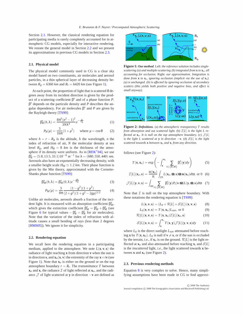
We recall here the rendering equation in a participatingmedium, applied to the atmosphere. We noteL(x,v, s) theradiance of light reachingx from directionv when the sun isin directions, andxo(x,v) the extremity of the rayx+tv (seeFigure1). Note thatxo is either on the ground or on the topatmosphere boundaryr = Rt . The transmittance Tbetweenxo andx, the radianceI of light reflected atxo, and the radi-anceJ of light scattered aty in direction−v are defined as

Figure 1: Our method. Left: the reference solution includes single-scattering (a) and multiple-scattering (b) integrated fromx to xo, allaccounting for occlusion.Right: our approximation. Integration isdone fromx to xs, ignoring occlusion (implicit via the use ofxs).(a) is unchanged. (b) is affected by ignoring occlusion of secondaryscatters (this yields both positive and negative bias, and effect issmall anyway).

Figure 2: Definitions. (a) the atmospheric transparency T resultsfrom absorption and out scattered light.(b) I[L] is the light L re-flected atxo. It is null on the top atmosphere boundary.(c) J [L]is the light L scattered aty in direction −v. (d) S[L] is the lightscattered towardsx betweenxo andx, from any direction.

follows (see Figure2):

T(x,xo) = exp

(

−∫ xo

x∑

i∈{R,M}

βei (y)dy

)

(5)

I[L](xo, s) =α(xo)

π

∫

2πL(xo,ωωω, s)ωωω.n(xo)dω, or 0 (6)

J [L](y,v, s) =

∫

4π∑

i∈{R,M}

βsi (y)Pi(v.ωωω)L(y,ωωω, s)dω (7)

Note thatI is null on the top atmosphere boundary. Withthese notations the rendering equation is [TS99]:

L(x,v, s) = (L0 +R[L]+S [L])(x,v, s) (8)

L0(x,v, s) = T(x,xo)Lsun, or 0 (9)

R[L](x,v, s) = T(x,xo)I[L](xo, s) (10)

S [L](x,v, s) =∫ xo

xT(x,y)J [L](y,v, s)dy (11)

whereL0 is the direct sunlightLsun attenuated before reach-ing x by T(x,xo). L0 is null if v 6= s, or if the sun is occludedby the terrain,i.e., if xo is on the ground.R[L] is the light re-flected atxo and also attenuated before reachingx, andS [L]is theinscatteredlight, i.e., the light scattered towardsx be-tweenx andxo (see Figure2).

2.3. Previous rendering methods

Equation8 is very complex to solve. Hence, many simpli-fying assumptions have been made in CG to find approxi-

c© 2008 The Author(s)Journal compilationc© 2008 The Eurographics Association and Blackwell Publishing Ltd.

E. Bruneton & F. Neyret / Precomputed Atmospheric Scattering

mate solutions that are easier to compute (see [Slo02] for asurvey). Most real-time methods ignore multiple scattering.In this case Equation8 reduces toL = L0 +R[L0] +S [L0].However, evenS [L0] is quite complex to solve. Some au-thors propose analytical solutions at the price of idealisa-tions: flat Earth with constant atmosphere density [HP02],or without Mie scattering [REK∗04]. The flat Earth hypoth-esis limits them to observers on the ground. Otherwise,S [L0]is generally computed by numerical integration [NSTN93],which can be done in real time using low sampling [O’N05].A notable exception is [SFE07] who rely on precomputa-tions of this integral. However, in order to reduce the num-ber of parameters, they only take into account the view andsun zenith angles, and neglect the angle between the viewand sun directions. Hence they cannot reproduce,e.g., theEarth’s shadow inside the atmosphere.

Ignoring multiple scattering as above is acceptable fordaylight but not for twilight [HMS05]. This is because sun-light traverses much less atmosphere during the day thanduring sunset or sunrise. Hence, some authors propose meth-ods to account for multiple scattering. [PSS99] fit the resultsof a double scattering Monte-Carlo simulation with an ana-lytical model, but their model is only valid for an observer onthe ground. [NDKY96] and [HMS05] use volume radiosityalgorithms to compute multiple scattering, but their methodsare far from real-time (minutes to hours per image).

In this paper we propose a new method to render the skyand the aerial perspective in real time, fromall viewpointsfrom ground to space, while takingmultiple scatteringintoaccount. It is inspired by [SFE07] and extends it with multi-ple scattering, with the previously ignored view-sun angleparameter, with a better parameterization for the precom-puted tables, and with a new method for light shafts.

3. Our method

For efficiency and realism, our goal is to precomputeL asmuch as possible, with only minimal approximations. Oursolution is based on an exact computation for zero and sin-gle scattering, and uses an approximation of occlusion ef-fects to compute multiple scattering. In fact we take the de-tailed ground shape into account for zero and single scatter-ing, in order to get correct ground colors, shadows and lightshafts. But we approximate it with a perfect sphere of con-stant reflectance to compute multiple scattering, to allow forprecomputation.

Notations Before presenting our method we need some no-tations and auxiliary functions. We noteL = L0+(R+S)[L]the solution of Equation8 for the case of a perfectly spher-ical ground of constant reflectanceα. L0, R, S, xo, I andso on are defined as before, but for this spherical ground.Note that thanks to the ground’s spherical symmetryx andvcan be reduced to an altitude and a view zenith angle. Hence

functions ofx,v, s such asL or S[L] can be reduced to func-tions of 4 parameters (2 forx,v and 2 fors). Note also thatL(resp.L) can be expressed with a series in the linear opera-torsR andS (resp.R andS), where theith term correspondsto light reflected and/or scattered exactlyi times:

L = L0 +(R+S)[L0]+ (R+S)[

(R+S)[L0]]

+ . . .

= L0 +L1 +L2 + . . . = L0 +L∗ (12)

Zero and single scattering We computeL0 andR[L0] ex-actly, during rendering. For this we use a shadowing algo-rithm to compute the sun occlusion (see Equation9), and aprecomputed table for the transmittanceT, which dependson only 2 parameters (see Section4). S [L0] is more compli-cated. It is an integral betweenx andxo but, due to the occlu-sion term inL0, the integrand is null at all pointsy that are inshadow (this is what gives light shafts). We suppose here thatthese points are betweenxs andxo (see Figure1 – the gen-eral case is discussed in Section5). Then the integral can bereduced to the lit segment[x,xs]. Moreover, occlusion can beignored since it is already accounted for viaxs, i.e., L0 canbe replaced withL0. This shows thatS [L0] =

∫ xsx TJ [L0].

By rewriting this as∫ xo

x TJ [L0]−∫ xo

xsTJ [L0], extending an

idea introduced in [O’N05] and reused in [SFE07], we fi-nally get a formulation using precomputable functions of 2and 4 parameters,T andS[L0]:

S [L0](x,v, s) = S[L0](x,v, s)−T(x,xs)S[L0](xs,v, s) (13)

Multiple scattering As shown aboveL0 andL1 can be com-puted exactly despite the occlusion. Unfortunately account-ing for occlusion in the other termsL2+ . . .=R[L∗]+S [L∗]is much more difficult. Hopefully, in this case the occlusioncan be approximated. Indeed, multiple scattering effects aresmall compared to single scattering during the day, whilethe ground contribution is small when it is not directly litby the sun. So we approximate occlusion effects inS [L∗]by integrating the contribution of multiple scattering, com-puted without occlusion, betweenx andxs. This yields bothpositive and negative bias (see Figure1). Mathematically,this approximation givesS [L∗] ≃

∫ xsx TJ [L∗]. We also ap-

proximate occlusion effects inR[L∗] with the ambient oc-clusion of an horizontal hemisphere due to the ground’s tan-gent plane,1+n.n

2 . This givesR[L∗]≃ R[L∗] with:

R[L∗] = T(x,xo)α(xo)

π1+n(xo).n(xo)

2E [L∗](xo, s) (14)

E [L∗](xo, s) =

∫

2πL∗(xo,ωωω, s)ωωω.n(xo)dω, or 0 (15)

By using the same rewriting rule as for Equation13, and bynotingS[L]|x = S[L](x,v, s), we finally get:

L≃ L0 +R[L0]+ R[L∗]+ S[L]|x−T(x,xs)S[L]|xs(16)

where the first three terms can be quickly computed with thehelp of precomputed 2D tables forT andE [L∗], and whereS[L] can be precomputed in a 4D table. We now show howto precompute them, in tables of a reasonnable size.

c© 2008 The Author(s)Journal compilationc© 2008 The Eurographics Association and Blackwell Publishing Ltd.

E. Bruneton & F. Neyret / Precomputed Atmospheric Scattering

Algorithm 4.1: PRECOMPUTE(norders)

T(x,v)← T(x, xo(x,v))∆E(x, s)← E [L0](x, s)∆S(x,v, s)← S[L0](x,v, s)E(x, s)← 0S(x,v, s)← ∆S(x,v, s)for i← 1 to i < norders

do

∆J(x,v, s)←J [T απ ∆E+∆S](x,v, s)

∆E(x, s)← E [T απ ∆E+∆S](x, s) = E [∆S](x, s)

∆S(x,v, s)← ∫ xox T(x,y)∆J(y,v, s)dy

E(x, s)← E(x, s)+∆E(x, s)S(x,v, s)← S(x,v, s)+∆S(x,v, s)

4. Precomputations

We precomputeT(x, xo(x,v)) for all x,v in a 2D tableT(x,v). Due to spherical symmetry,T depends only onr = ‖x‖ andµ= v.x/r [O’N05]. As [O’N05], we then use theidentityT(x,y) = T(x,v)/T(y,v), with v = (y−x)/‖y−x‖.

We precomputeE [L∗] andS[L] in two tablesE andS withan algorithm that computes each scattering orderLi one afterthe other. This algorithm uses three intermediate tables∆E,∆S and∆J containing after each iterationi E [Li ], S[Li] andJ [Li]. ∆E and∆S are added to the result tablesE andS atthe end of each iteration (R is computed with the identityR[L](x,v, s) = T(x, xo)

απ E [L](xo, s) – see Algorithm4.1).

Angular precision SinceS is a 4D table its size increasesvery quickly with resolution. So we can only use a lim-ited angular resolution forv. This poses a precision prob-lem, which is however limited to the strong forward Miescattering. In order to solve it we separate the single Miescattering term from all the others inS, so as to applythe phase function at runtime. For this we rewriteS[L] asPMSM[L0]+PRSR[L0]+ S[L∗]. We then storeCM = SM[L0]andC∗ = SR[L0] + S[L∗]/PR separately, which requires 6values per entry inS. If necessary, for efficiency, this can bereduced to 4 values per entry by storing only the red com-ponentCM,r of CM . In this case the other components canbe approximated with a proportionality rule betweenSM[L0]

andSR[L0], which givesCM ≃C∗CM,rC∗,r

βsR,r

βsM,r

βsM

βsR

.

Parameterization In order to storeS[L] into S we need amapping from(x,v, s) into table indices in[0,1]4. A simplesolution is to user = ‖x‖ and the cosinus of the view zenith,sun zenith, and view sun angles,µ = v.x/r, µs = s.x/r andν = v.s (mapped linearly from[Rg,Rt ]× [−1,1]3 to [0,1]4).

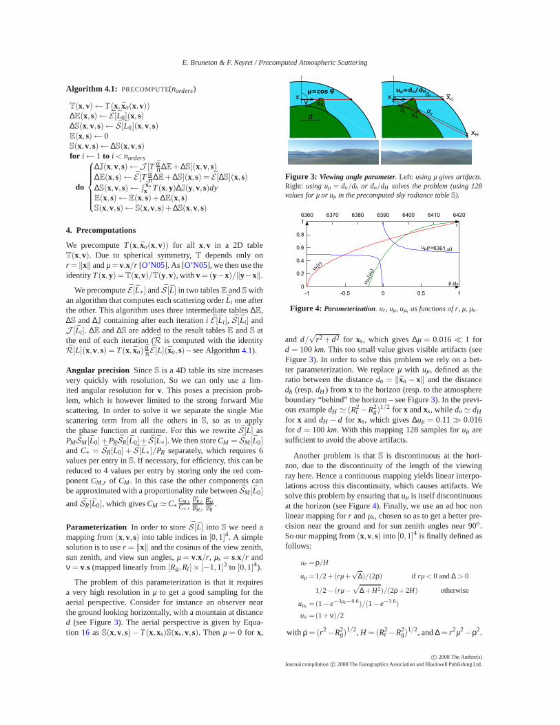
The problem of this parameterization is that it requiresa very high resolution inµ to get a good sampling for theaerial perspective. Consider for instance an observer nearthe ground looking horizontally, with a mountain at distanced (see Figure3). The aerial perspective is given by Equa-tion 16 asS(x,v, s)−T(x,xs)S(xs,v, s). Thenµ = 0 for x,

Figure 3: Viewing angle parameter. Left: using µ gives artifacts.Right: using uµ = do/dh or do/dH solves the problem (using 128values for µ or uµ in the precomputed sky radiance tableS).

Figure 4: Parameterization. ur , uµ, uµs as functions of r, µ, µs.

and d/√

r2 +d2 for xs, which gives∆µ = 0.016≪ 1 ford = 100km. This too small value gives visible artifacts (seeFigure3). In order to solve this problem we rely on a bet-ter parameterization. We replaceµ with uµ, defined as theratio between the distancedo = ‖xo− x‖ and the distancedh (resp.dH ) from x to the horizon (resp. to the atmosphereboundary “behind” the horizon – see Figure3). In the previ-ous exampledH ≃ (R2

t −R2g)

1/2 for x andxs, while do≃ dH

for x anddH − d for xs, which gives∆uµ = 0.11≫ 0.016for d = 100 km. With this mapping 128 samples foruµ aresufficient to avoid the above artifacts.

Another problem is thatS is discontinuous at the hori-zon, due to the discontinuity of the length of the viewingray here. Hence a continuous mapping yields linear interpo-lations across this discontinuity, which causes artifacts. Wesolve this problem by ensuring thatuµ is itself discontinuousat the horizon (see Figure4). Finally, we use an ad hoc nonlinear mapping forr andµs, chosen so as to get a better pre-cision near the ground and for sun zenith angles near 90o.So our mapping from(x,v, s) into [0,1]4 is finally defined asfollows:

ur =ρ/H

uµ =1/2+(rµ+√

∆)/(2ρ) if rµ < 0 and∆ > 0

1/2− (rµ−√

∆ + H2)/(2ρ+ 2H) otherwise

uµs =(1−e−3µs−0.6)/(1−e−3.6)

uν =(1+ ν)/2

with ρ = (r2−R2g)

1/2, H = (R2t −R2

g)1/2, and∆ = r2µ2−ρ2.

c© 2008 The Author(s)Journal compilationc© 2008 The Eurographics Association and Blackwell Publishing Ltd.

E. Bruneton & F. Neyret / Precomputed Atmospheric Scattering

Figure 5: Evaluation of l. Left: due to the false boundaries b andc, the computed length∆z−∆n.zg = zg−za+zc−zb is larger than l.Clamping this value to zg− zmin fixes the problem.Right: viewpointin shadow. Using only the extruded edges,xo would be seen as litand l would be equal to0 instead of zg − znear. Projecting the backfaces (dashed line) on the near plane solves the issue [HHLH05].

5. Rendering

In order to render the sky and the aerial perspective we evalu-ate Equation16at each pixel.L0 can be efficiently computedusingT. ComputingR[L0] involvesT, α(xo) andn(xo), anda shadow test to determine whetherxo is lit. Finally E andS are used to computeR[L∗] andS[L]. As in [SFE07], x isthe camera position or, if in space, the nearest intersectionof the viewing ray with the atmosphere boundary. The onlyremaining non-trivial parameter isxs, which depends on theterrain shadows and gives light shafts.

Most light shaft algorithms use sampling or slicing to per-form a numerical integration along the viewing ray, with ashadow map to find which samples are lit. Up to 100 sam-ples per ray must be used to eliminate the artifacts due to thediscrete sampling [IJTN07]. We propose here a new methodinspired from shadow volumes [HHLH05]. It does not relyon numerical integration, and therefore does not suffer fromthese artifacts. We first show that an exact computation ispossible but not adapted to the GPU. We then present an ap-proximate solution better adapted to the GPU. Our idea isto use the precomputed integralS to compute the inscatteredlight due to each lit segment[xi ,xi+1] along the viewing ray,which is given byT(x,xi)S|xi

−T(x,xi+1)S|xi+1. By defini-

tion the pointsxi are on the boundaries of the shadow volumeof the terrain. Hence they can be found with a shadow vol-ume algorithm such as [HHLH05]. This algorithm extrudesthe silhouette edges of objects, as seen from the light; it alsoprojects these objects on the near plane to get correct re-sults despite clipping. However these algorithms also gen-erate many surfaces that do not correspond to a boundarybetween light and shadow (see Figure5). These false bound-aries must be ignored when computing the inscattered light,otherwise a wrong result is obtained. Unfortunately, detect-ing them is a non local operation that is not adapted to GPU(requiring,e.g.,the use of multiple passes, or list structures).

Our solution is to use the shadow volume algorithm tocompute the total lengthl of the shadowed segments, andto replace them with a single segment of this length at the“ground” end of the ray (see Figure5). The false boundariesstill cause problem,i.e., an overestimation ofl . Here how-

Figure 6: Validation. The sky luminanceS in fisheye view for sev-eral sun zenith angles, in color, and relatively to the zenith lumi-nance. Withα = 0.1, βs

M = 210−5 m−1, βsM/βe

M = 0.9, g = 0.76and HM = 1.2 km we get the CIE clear sky model, fitted from actualmeasurements (source [ZWP07]).

ever l can be clamped to the distance between the nearestand farthest faces of the shadow volume. This gives the cor-rect result in most cases, and an approximate value in theothers. Our detailed algorithm is the following. We associatewith each pixel 4 values∆n, ∆z, zmin, zmax initialized to 0, 0,∞, 0. In a first step we decrement (resp. increment)∆n by1 and∆z by the fragment depthz, and updatezmin andzmax

with z, for each front (resp. back) face of the shadow surface.In a second step we use (see Figure5)

l = clamp(∆z−∆n.zground,0,zground− zmin)

L≃ L0 +R[L0]+ R[L∗]+S|x−T(x,xs)S|xs=xo−lv (17)

when looking at the ground or, when looking at the sky:

l = clamp(∆z,0,zmax)

L≃ L0 +R[L0]+ R[L∗]+T(x,xs)S|xs=x+lv (18)

6. Implementation, results and discussion

Precomputations We have implemented the precomputa-tion algorithm on GPU, with fragment shaders processingthe numerical integration. This is not mandatory but it allowsus to quickly change atmospheric parameters, and it savesdisk space (indeed 5 scattering orders are computed in 5sec-ondson a NVidia 8800 GTS). We storeT(r,µ) andE(r,µ) in64×256 and 16×64 textures. We storeS(ur ,uµ,uµs,uν) =[C∗,CM,r ] in a 32×128×32×8 table, seen as 8 3D tablespacked in a single 32× 128× 256 RGBA texture (using amanual linear interpolation for the 4th coordinate). Thanksto our optimized parameterization our 4D table has a betterprecision and uses less space than the 3D table of [SFE07](8 MB for S with 16 bits floatsvs12 MB for their 1283 tex-ture).

Rendering The rendering is done in four passes:

• we draw the terrain in the depth buffer only;• we draw the shadow volume of the terrain into a∆n, ∆z,

zmin, zmax texture. For this we use theADD andMAX blend-ing functions, disable depth write, and use a geometryshader that extrudes the silhouette edges (as seen from thesun). This shader also projects on the near plane along−s

c© 2008 The Author(s)Journal compilationc© 2008 The Eurographics Association and Blackwell Publishing Ltd.

E. Bruneton & F. Neyret / Precomputed Atmospheric Scattering

the back faces (as seen from the sun) that are between thisplane and the sun [HHLH05];

• we draw the terrain and the other objects with aerial per-spective, as well as the sky, using Equations17 and18.If there are transparent objects such as clouds, aerial per-spective must be computed for each object, before blend-ing. We use∆n to compute occlusion inR[L0], andl com-puted as above to getxs (see Section5);

• we finally apply a global tone mapping function.

Results We run several tests with a height field and a re-flectance texture from Nasa’s Earth Observatory [SVS∗05].Results are depicted in Figures8 and9. As shown in Fig-ures6 and7 our model can reproduce with good accuracythe CIE clear sky model, fitted from actual measurements atthe ground level [DK02]. Since the sky color and aerial per-spective are computed with a few texture fetches per pixel(< 10), our algorithm is quite fast. For instance, for the rightview in Figure8 in 1024×768, we get 125 fps without lightshafts on a NVidia 8800 GTS. This includes 5 ms for the un-shaded terrain, 0.4 ms for the first three terms in Equations17 and 18 and 2.6 ms for the remaining terms (including1 ms to evaluate the non linear parameterization). We get25 fps with light shafts (i.e., the first two rendering passescost a lot, about 32 ms). By comparison, we get 50 fps withour reimplementation of [O’N05], using ten samples per ray(to get the same quality for single scattering, without shafts).

Limitations A limitation of our method is that the aerosolproperties are assumed constant, depending only on altitude,whereas in fact they can greatly change depending on theatmospheric conditions [Slo02]. Since our precomputationsare very fast we can change these properties quickly, but theyremain uniform.

7. Conclusion

We have presented the first real-time method to render thesky and the aerial perspective from all viewpoints, with mul-tiple scattering, terrain shadows and light shafts, and correctvariation with all view and sun angles. This method is basedon minimal simplifying assumptions that allow us to get anapproximate solution of the rendering equation, in whichmost terms can be precomputed. This method can easily beextended to more complex physical models, with more con-stituents or more wavelengths.

As future work we would like to model the effect ofclouds on the ground illuminance and on the aerial per-spective, to remove the clear sky hypothesis. Indeed withmany clouds the interreflections between the ground and theclouds should be taken into account [BNL06]. And their ef-fect on aerial perspective should also be considered. To ourknowledge, this has never been done.

The source code of our implementation is available athttp://evasion.inrialpes.fr/~Eric.Bruneton/.

Acknowledgments This work was partially funded by theNatsim ANR ARA project. We would like to thank AntoineBouthors and Cyril Soler for proofreading.

References

[BNL06] BOUTHORSA., NEYRET F., LEFEBVRES.: Real-timerealistic illumination and shading of stratiform clouds. In Euro-graphics Workshop on Natural Phenomena(sep 2006).

[DK02] DARULA S., KITTLER R.: CIE general sky standarddefining luminance distributions.eSim(2002).

[HHLH05] HORNUS S., HOBEROCK J., LEFEBVRE S., HART

J. C.: ZP+: correct Z-pass stencil shadows. InACM Sympo-sium on Interactive 3D Graphics and Games (I3D)(April 2005),ACM, ACM Press.

[HMS05] HABER J., MAGNOR M., SEIDEL H.-P.: Physically-based simulation of twilight phenomena.ACM Trans. Graph. 24,4 (2005), 1353–1373.

[HP02] HOFFMAN N., PREETHAM A. J.: Rendering outdoorlight scattering in real time.Proceedings of Game DeveloperConference(2002).

[IJTN07] IMAGIRE T., JOHAN H., TAMURA N., NISHITA T.:Anti-aliased and real-time rendering of scenes with light scat-tering effects.Vis. Comput. 23, 9 (2007), 935–944.

[NDKY96] N ISHITA T., DOBASHI Y., KANEDA K., YA-MASHITA H.: Display method of the sky color taking into ac-count multiple scattering. InProceedings of Pacific Graphics(1996), pp. 117–132.

[NSTN93] NISHITA T., SIRAI T., TADAMURA K., NAKAMAE

E.: Display of the Earth taking into account atmospheric scatter-ing. In SIGGRAPH 93(1993), ACM, pp. 175–182.

[O’N05] O’N EIL S.: Accurate atmospheric scattering. InGPUGems 2: Programming Techniques for High-Performance Graph-ics and General-Purpose Computation(2005), Addison-WesleyProfessional.

[PSS99] PREETHAM A. J., SHIRLEY P., SMITS. B. E.: A prac-tical analytic model for daylight. InSIGGRAPH 99(1999).

[REK∗04] RILEY K., EBERT D. S., KRAUS M., TESSENDORF

J., HANSEN C. D.: Efficient rendering of atmospheric phenom-ena. InRendering Techniques(2004), pp. 374–386.

[SFE07] SCHAFHITZEL T., FALK M., ERTL T.: Real-time ren-dering of planets with atmospheres. InWSCG International Con-ference in Central Europe on Computer Graphics, Visualizationand Computer Vision(2007).

[Slo02] SLOUP J.: A survey of the modelling and rendering of theEarth’s atmosphere. InSCCG ’02: Proceedings of the 18th springconference on Computer graphics(2002), ACM, pp. 141–150.

[SVS∗05] STOCKLI R., VERMOTE E., SALEOUS N., SIMMON

R., HERRING D.: The Blue Marble Next Generation – a truecolor Earth dataset including seasonal dynamics from MODIS.NASA Earth Observatory(2005).

[TS99] THOMAS G. E., STAMNES K.: Radiative transfer in theatmosphere and ocean. Cambridge Univ. Press, 1999.

[ZWP07] ZOTTI G., WILKIE A., PURGATHOFERW.: A criticalreview of the Preetham skylight model. InWSCG 2007 ShortCommunications Proceedings I(Jan. 2007), pp. 23–30.

c© 2008 The Author(s)Journal compilationc© 2008 The Eurographics Association and Blackwell Publishing Ltd.

E. Bruneton & F. Neyret / Precomputed Atmospheric Scattering

0

0.2

0.4

0.6

0.8

1

-80 -60 -40 -20 0 20 40 60 80

Rel

ativ

e sk

y lu

min

ance

(su

n ze

nith

ang

le =

0)

View angle

CIE ModelOur Model

0

0.2

0.4

0.6

0.8

1

1.2

1.4

1.6

-80 -60 -40 -20 0 20 40 60 80

Rel

ativ

e sk

y lu

min

ance

(su

n ze

nith

ang

le =

10)

View angle

CIE ModelOur Model

0

0.5

1

1.5

2

2.5

3

-80 -60 -40 -20 0 20 40 60 80

Rel

ativ

e sk

y lu

min

ance

(su

n ze

nith

ang

le =

20)

View angle

CIE ModelOur Model

0

0.5

1

1.5

2

2.5

3

3.5

4

-80 -60 -40 -20 0 20 40 60 80

Rel

ativ

e sk

y lu

min

ance

(su

n ze

nith

ang

le =

30)

View angle

CIE ModelOur Model

0

1

2

3

4

5

6

-80 -60 -40 -20 0 20 40 60 80

Rel

ativ

e sk

y lu

min

ance

(su

n ze

nith

ang

le =

40)

View angle

CIE ModelOur Model

0

1

2

3

4

5

6

7

8

9

10

-80 -60 -40 -20 0 20 40 60 80

Rel

ativ

e sk

y lu

min

ance

(su

n ze

nith

ang

le =

50)

View angle

CIE ModelOur Model

0

2

4

6

8

10

12

14

16

18

-80 -60 -40 -20 0 20 40 60 80

Rel

ativ

e sk

y lu

min

ance

(su

n ze

nith

ang

le =

60)

View angle

CIE ModelOur Model

0

5

10

15

20

25

30

35

-80 -60 -40 -20 0 20 40 60 80

Rel

ativ

e sk

y lu

min

ance

(su

n ze

nith

ang

le =

70)

View angle

CIE ModelOur Model

0

10

20

30

40

50

60

-80 -60 -40 -20 0 20 40 60 80

Rel

ativ

e sk

y lu

min

ance

(su

n ze

nith

ang

le =

80)

View angle

CIE ModelOur Model

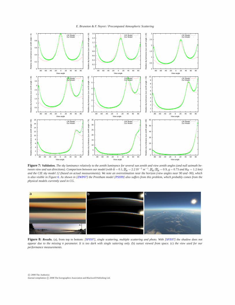
Figure 7: Validation. The sky luminance relatively to the zenith luminance for several sun zenith and view zenith angles (and null azimuth be-tween view and sun directions). Comparison between our model (with α = 0.1, βs

M = 2.210−5 m−1, βsM/βe

M = 0.9, g= 0.73and HM = 1.2 km)and the CIE sky model 12 (based on actual measurements). We note an overestimation near the horizon (view angles near 90 and -90), whichis also visible in Figure6. As shown in [ZWP07] the Preetham model [PSS99] also suffers from this problem, which probably comes from thephysical models currently used in CG.

Figure 8: Results.(a), from top to bottom:[SFE07], single scattering, multiple scattering and photo. With [SFE07] the shadow does notappear due to the missingν parameter. It is too dark with single sattering only.(b) sunset viewed from space.(c) the view used for ourperformance measurements.

c© 2008 The Author(s)Journal compilationc© 2008 The Eurographics Association and Blackwell Publishing Ltd.

E. Bruneton & F. Neyret / Precomputed Atmospheric Scattering

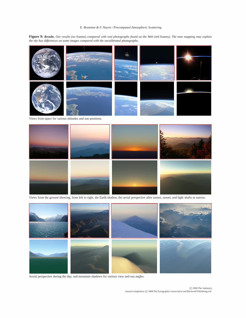
Figure 9: Results.Our results (no frames) compared with real photographs found on the Web (red frames). The tone mapping may explainthe sky hue differences on some images compared with the uncalibrated photographs.

Views from space for various altitudes and sun positions.

Views from the ground showing, from left to right, the Earth shadow, the aerial perspective after sunset, sunset, and light shafts at sunrise.

Aerial perspective during the day, and mountain shadows forvarious view and sun angles.

c© 2008 The Author(s)Journal compilationc© 2008 The Eurographics Association and Blackwell Publishing Ltd.