Proceedings of the 5th IIAE International Conference on Industrial Application Engineering 2017

© 2017 The Institute of Industrial Applications Engineers, Japan.

The Evaluation of Cornering Behavior of Low Floor Electric Bus: the

Effected to Mass Distribution and Friction Coefficient

Ekalak Prompakdeea, Pornporm Boonpormb, Supakit Rooppakhunb,*

aSchool of Manufacturing Engineering, Institute of Engineering, Suranaree University of Technology,

Nakhonratchasima, 30000 Thailand. bSchool of Machanical Engineering, Institute of Engineering, Suranaree University of Technology, Nakhonratchasima,

30000 Thailand.

*Corresponding Author: supakit@sut.ac.th

Abstract

The Low Floor electric bus, which had been promoted

by the Government of Thailand, boost design technologies

and research in the automotive industry. In order to fulfill the

safety requirements regulated by the Department of Land

Transport of Thailand, it must undergo both static and

dynamic analysis. The vehicle dynamic cornering behavior

plays an important role to demonstrate handling stability

especially for active safety. In this paper, we study effect of

the parameters of weight distribution and the road friction

coefficient, which were indicated in terms of understeer

gradient. The analysis had been conducted by ADAM CARS

based on the vehicle’s multi-body model. The analysis was

applied under steady state cornering conditions based on

three front to rear weight distribution configurations in

percent of 50/50, 45/55 and 40/60, and a lateral tire road

friction coefficient of 0.5, 0.7 and 0.9. The results show that

the greater the friction coefficient between road and tire, the

better handling behavior. The trends are in the same fashion

when the three weight distributions are varied and the 40/60

configuration has the smallest understeer gradient. But in the

real design we should consider other behavior like ride

performance and static analysis, so that the configuration of

45/55 is chosen in our real design.

Keywords: Center of Gravity, Cornering Dynamic, Low

Floor Electric Bus, Understeer gradient, Bus handling.

1. Notation

In this paper, the following notation is used throughout:

f = Slip angle of the front tire

r = Slip angle of the rear tire

= Side slip angle of vehicle

= Front wheel steering angle

ya = Lateral acceleration at vehicle C.G.

fC = Effective cornering stiffness of the Front axle

rC = Effective cornering stiffness of the rear axle

K = Understeer gradient

L = Wheelbase

fm = Front axle weight

rm = Rear axle weight

R = Turning radius

V = Vehicle speed

m = Total mass

= Friction coefficient

yF = The lateral force

zF = The normal force

g = Gravitational acceleration

= Yaw angle

= Yaw rate

y = Lateral slip acceleration

DOI: 10.12792/iciae2017.046 254

2. Introduction

Concerning mass transportation, a number of countries

have researched and developed a bus industry. So do

Thailand, domestic electric buses are promoted for design

and development tasks in order to achieve the main goals like

performance as well as safety issues.

Referring to the statistics from the Department of

Transport of Thailand, there are approximately 80,000

busses per year which have registered to serve more than 35

million passengers traveling by bus. Consequently, traffic

accidents are occurred by evaluating damage and dead about

600 million baht [1]. For this reason, in the bus design

process, both static and dynamic behaviors analysis is

required to indicate the safety of the bus. The static stability

test relates to the vehicle’s resistance to rollover, which

involves a pose of center of gravity.

The parameters of vehicle weight distribution can be

designed and calculated via the position of battery, air

condition, axle and other component. In the case of vehicle

dynamics, the subject deals with the study of vehicle

response related to driver input, ability of the vehicle to

stabilize its motion against external disturbances for purpose

of handling characteristics, especially cornering dynamic

characteristic[2] (e.g., lateral acceleration, side slip angle,

Yaw rate and understeer gradient) [3, 4].

This study is aimed at evaluating the cornering dynamic

characteristics of the Low Floor Electric bus under the effect

of mass distribution. The analysis had been applied by

ADAM CARS [5] based vehicle multi-body model under

thee steady state cornering conditions. Three possible

configurations front/rear axle weight distribution (in percent)

of 50/50, 45/55 and 40/60 are taken into account as well as

the variation of the friction coefficient in the wet to dry road

condition of 0.5, 0.7 and 0.9. The handling characteristics

are mainly determined from understeer gradient wheel slip

angle and yaw rate. [7, 8] The understeer gradient could be

evaluated by operating the vehicle around a constant radius

turn by observing steering angle versus lateral acceleration.

3. Problem Definition

The evaluation of the cornering dynamic behavior of

buses [9] plays an important role to make it capable of

operating in the most of road condition safely. So that there

are the cooperation between bus manufacturer Cherdchai

industrial co.ltd and Suranaree University of Technology for

design and development of electric bus in the theme of

weight distribution during steady state condition.

4. Steady State Vehicle Cornering Condition

To explain the cornering characteristic, a simple bicycle

model is considered in order to identify the kinematics

characteristics among the parameters like lateral,

longitudinal as well as yaw dynamics. In figure 1, X- Y

reference coordinate frame is defined using compass

directions (e.g. east and north) and an x- y rotating frame at

the vehicle’ s center of gravity in longitudinal and lateral

dynamics respectively. In plane kinematics, one of the

rotation angle about z-axis, called yaw angle ( ), was taken

into account.

To define the relationship between the fixed frame X- Y

and the rotating frame x- y, the acceleration analysis was

perform. The acceleration of the vehicle in global coordinate

frame is defined as

yxrxrxrxxa

2 (1)

And the lateral acceleration is

2a R yy (2)

The term y is interesting because it shows that the vehicle

slip behavior and it cannot be negligible in some case of

operation as discuss later.

IC

rl

fl

C

V

X

Y

f

r

R

L

x

y

Fig. 1. Steady state vehicle cornering condition.

Steady state cornering is implemented to verify the

handling characteristic which is aimed at understeer gradient.

As shown in figure 1, the front and rear wheel slip angle,

denoted by f and

r respectively, are defined as the

angle between the longitudinal axis of the wheel and the

255

velocity vector. The instantaneous turn centre IC of the

vehicle is the point at which the two lines perpendicular to

the velocities of the two wheels meet. It is assumed

throughout that the road radius is much larger than the wheel

base of the vehicle. From this geometry, we approximate a

kinematics relationship for the wheel steering angle as:

f r

L

R (3)

Fig. 2. Lateral Force acting on the vehicle and the

components of friction force at each wheels [12].

yx

y maR

VmF

2

(4)

Considering the dynamics model of the vehicle mentioned in

figure 2, there are lateral forces acted on the tires due to the

centripetal action during cornering following equation 4 so

that the wheel side slip angle, f and

r are varied to

the lateral tries force. Assuming the small slip condition, the

lateral tire force is proportional to its slip angle with the

constant called cornering stiffness and they are denoted for

the front and rear as fC and rC respectively.

The steady state steering angle in equation 3 then can be

rewritten as:

2

2 2

f xr

f r

f r

m VmL L

R R C C R

(5)

Or equivalently:

y

LKa

R (6)

Where K is understeer gradient, In case of understeer

K should greater than zero due to a larger slip angle at the

front tires compared to the rear tires. The relationship

between weight transfer and wheel slip angle is interpreted

in following equation 7.

f r

f r

f r

m m

C C (7)

The coefficient of friction is concerned the contact

surface between tire and ground. The faster the vehicle

negotiates a bend, the higher the coefficient of friction used

to prevent the undesired understeer behavior.

5. Multi-Body Dynamic Simulation

A multi body dynamic (MBD) system is a simulation

modeling method, consisting of solid bodies, or links, that

are connected to each other by joints that restrict their

relative motion. Motion analysis is important because

product design frequently requires an understanding of how

multiple moving parts interact with each other and their

environment. From automobiles and aircraft to washing

machines and assembly lines moving parts generate loads

that were often difficult to predict. Complex mechanical

assemblies present design challenges that require a dynamic

system level analysis to be met.

To study the cornering dynamic behavior of buses under

steady state and transient state conditions, multi-body model

of the bus had been built in MSC ADAMS CARS software

tool. The multi-body bus model was built based on the

specification in Table 1.

Table 1. Specification of Low Floor Electric Bus.

Parameters Bus Model

GVW 18,000 kg.

Total Weight 12,530 kg.

Front Axle Weight 5,750 kg.

Rear Axle Weight 6,780 kg.

Overall Length 12 m.

Wheelbase 6.5 m.

Track Width Front 2,096 mm.

Rear 1,800 mm.

Suspension Front Air Suspension

Rear Air Suspension

Tires 275/70 R22.5

256

Fig. 3. Low Floor Electric Bus model.

5.1 The Virtual Low Floor Electric Bus

According to the virtual model of the Low Floor Electric

bus model, the multi- body dynamic modelling had been

carried out in MSC ADAMS/Truck tool ( MSC software) .

The virtual model consisted of the sub- systems in the Low

Floor Electric bus specification, with the center of gravity

from experiments shown in figure 4.

Fig. 4. Experimental of Center of Gravity (CG.)

From the experiment realting to the center of gravity, the

front axle weight was found to be 5,750 kg, and the rear axle

weight was 6,780 kg, giving the weight distribution % ( F/R)

of 45/55. For the height of center of gravity, it was necessary

to use the static stability factor ( SSF) , which is an at rest

calculation of the roll- over resistance based on exterior

dimension of vehicle. The SSF formula is

/ 2SSF t h (8)

Where t is the track width of the vehicle (mm), and h is the

height of center of gravity (mm). The SSF of pick-up trucks,

vans and buses will be in the range of 1 to 1. 3. For the

purpose of calculations herein, it is assumed to be 1.

20961

2 2

tSSF

h h

20961048

2h mm

Fig. 5. Location of Center of Gravity (CG.)

Table 2. show the weight distribution of Low Floor Electric

bus model and the distance of CG position from front axle in

this study.

The basic information required to understand multi-

body dynamic simulation is its mathematical formulation. It

explains how lateral forces are generated while a vehicle is

turning, and their relation with the slip angle and lateral

acceleration, as well as understeer gradient. The Low Floor

Electric bus model was used to estimate vehicle handling

characteristics required for the model.

5.2 Simulation condition

The vehicle dynamic test under steady state condition

was simulated virtually on a constant radius cornering test.

The aim of this test was to assess the lateral acceleration, side

slip angle, Yaw rate and understeer gradient of different

configurations of virtual model. The characteristics of the

test vehicle were investigated in a total of nine conditions:

three friction coefficients (0. 5, 0. 7, and 0. 9) [ 11] at each of

three different weight distributions (front/ rear axle weight in

percent, as 55/45, 50/50 and 45/55). For the test, the vehicle

models were maneuvered on the test track at initial

longitudinal velocity 10 km/h for left turn. The data were

carried out by 0. 1 interval time up to 45 km/ h under 50

seconds on the flat track.

5.3 Lateral Friction Coefficient

Table 2. The Weight Distribution of Low Floor Electric

Bus.

Layout Distant form

Front axle

% WD (F/R)

CG.1 3250 mm. 50/50

CG.2 3520 mm. 45/55

CG.3 3900 mm. 40/60

257

The lateral coefficient of friction relates to the ease with

which a vehicle will skid on a road. It is the ratio between the

lateral force and the normal force acting on the contact point,

given by:

y

z

F

F (9)

The maximum lateral friction coefficient is related to the

maximum forces that the tires can provide. It corresponds to

the value where the lateral force reaches saturation and there

is a risk of an exit route. Maximum friction was largely

related to road conditions and effects between the tire and the

road. It was an indication of road status and possible loss of

adhesion. This parameter cannot be measured by

conventional sensors, so it requires an estimation technique

for its estimation based on available measurements and

tire/ road interaction models. The true values of friction

coefficient used by the simulator in the generation of the

dynamic parameters, for a dry road the maximum friction

coefficient is 0. 9 and wet road the maximum friction

coefficient is 0.6 [11].

6. Results and Discussion

Under steady state cornering investigation, the lateral

acceleration consists of two components as described in

equation ( 2) it was evidenced that the lateral acceleration

yaw rate and vehicle speed can be measured and calculated.

Both were not equal because of the lateral slip acceleration

cannot be measured directly, but by comparison. Its value

occurs and leads to instability in the real world. Figure 6

demonstrates the components among them. From each test

condition, the result show that the more increase of bus

speed, the more gap between them or slip accelerations were

raised and there were in the same fashion.

15 20 25 30 35 40 45

0

0.2

0.4

0.6

0.8

1

Speed (km/h)

Accele

ration (

g)

ya

V

Fig. 6. Components of acceleration

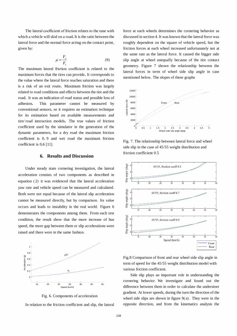
In relation to the friction coefficient and slip, the lateral

force at each wheels determines the cornering behavior as

discussed in section 4. It was known that the lateral force was

roughly dependent on the square of vehicle speed, but the

friction forces at each wheel increased unfortunately not at

the same rate as the lateral force. It caused the bigger side

slip angle at wheel unequally because of the tire contact

geometry. Figure 7 shown the relationship between the

lateral forces in term of wheel side slip angle in case

mentioned below. The slopes of these graphs

0 0.5 1 1.5 2 2.5 3 3.5 4 4.5 50

2000

4000

6000

8000

10000

12000

Wheel side slip angle (deg)

Late

ral fo

rce (

N)

Front Rear

Fig. 7. The relationship between lateral force and wheel

side slip in the case of 45/55 weight distribution and

friction coefficient 0.5

Fig.8 Comparison of front and rear wheel side slip angle in

term of speed for the 45/55 weight distribution model with

various friction coefficient.

Side slip plays an important role in understanding the

cornering behavior. We investigate and found out the

difference between them in order to calculate the understeer

gradient. At lower speeds, during the turn the direction of the

wheel side slips are shown in figure 9( a) . They were in the

opposite direction, and from the kinematics analysis the

258

velocity vector of the vehicle makes it behave like

understeer. In contrast, in figure 9( b) at higher speed, the

rear wheel slip was in the same direction as rear wheel slip

angle, causing the bus to also understeer with higher

understeer gradient.

(a)

(b)

Fig. 9. Front and rear side slip during (a) lower speed 10-30

km/h and (b) higher speed 30-45 km/h

0.1 0.15 0.2 0.25 0.37

7.2

7.4

7.6

7.8

Lateral acceleration (g)

Fro

nt

wheel ste

ering a

ngle

(deg)

Lower speed

Higher speed

Fig. 10 The relationship between front wheel steering

angle and the lateral acceleration.

Based on the result of steady state vehicle dynamic test,

the understeer gradient by varying CG and friction

coefficient were evaluated. Understeer gradients were

derived from equation ( 5) by evaluating the slope of the

graph ( in figure 10. ) between front wheel steering angle

versus lateral acceleration. The trend seems to be nonlinear

but it was approximated as bilinear curve during low speed

and high speed criteria, as stated in table 3 and 4.

Both table 3 and 4 displayed the comparison of weight

distribution and friction coefficient .The decrease in weight

distribution F/R ratio as 50/50 45/55 and 40/60 affect minor

change in understeer gradient. Unlike the variation of friction

coefficient, it was obviously shown the better handling

behavior. By the way all values are acceptable based on our

experience of handling behavior. .................

Fig. 11 The relationship between understeer gradient

and friction and the weight ratio at velocity 10-30 km/h.

Table 3. Understeer gradient of each layout in fiction

condition at velocity 10-30 k/h.

Layout % WD

(F/R)

Understeer Gradient (deg/g)

0.5 0.7 0.9

CG.1 50/50 2.12 1.97 1.92

CG.2 45/55 2.05 1.94 1.85

CG.3 40/60 1.74 1.51 1.48

Table 4. Understeer gradient of each layout in fiction

condition at velocity 30-45 k/h.

Layout % WD

(F/R)

Understeer Gradient (deg/g)

0.5 0.7 0.9

CG.1 50/50 3.24 2.42 2.20

CG.2 45/55 3.14 2.38 2.18

CG.3 40/60 2.74 1.86 1.62

259

Fig. 12 The relationship between understeer gradient

and friction and the weight ratio at velocity 30-45 km/h.

7. Conclusion

Considering the multi-body dynamic simulation, we

studied the effect of weight distribution and friction

coefficient in steady state cornering condition. The vehicle

handling characteristic of Low floor electric bus was

performed via understeer gradient. The effect of various

friction coefficients are significantly in the same pattern when

varying the weight transfer configuration. The greater value

of the coefficient leads the bus better handling. The weight

distribution in format 40/60 seems to be the best understeer

gradient in compare to three models. But in the real design we

choose the 45/55 because of compromising other condition

like ride performance. In this study, the center of gravity at

low speed and higher speeds was not over than the value from

literature review. So that for propose in bus design process

should be realized require to know the weight of bus

component and design to get the highest balance of the bus.

Acknowledgment

The authors would like to acknowledge Suranaree

University of Technology, National Metal and Materials

Center for the sincere and also thank Cherdchai Industrial ltd.

for support among the research activities of this article

References

(1) Transport Statistics Sub-Division, Planning Division :

http://apps.dlt.go.th/statistics_web/statistics.html,

Retrieved on November 30, 2016

(2) Gillespie TD : “Fundamentals of vehicle dynamics

SAE”, Warrendale, 1992

(3) H. H. Kim and J. Ryu : “Sideslip Angle Estimation

Considering Short-duration Longitudinal Velocity

Variation", Int. J. of Auto. Tech., vol. 12(4), pp.545-553,

July 2011

(4) M. Sherman and G. Myers : “Vehicle Dynamics

Simulation for Handling Optimization of Heavy Trucks,”

SAE Technical Paper 2000-01-3437, Dec. 2000,

doi:10.4271/2000-01-3437

(5) S. Murthy, M. Gowda and H. Venna : “Evaluation of

Handling Characteristics of an Intercity Bus by Multi-

Body Dynamic Simulations”, SAE Technical Paper

2016-28-0178, 2016, doi:10.4271/2016-28-0178

(6) H. Mazumder, M.M.AI Emran, M. Ekterabi and A.

Kapoor : “Effect of mass distribution on cornering

dynamic of retrofitted EV”, Energy Procedia 14, 2012

(7) J. S. Jo, S. H. You, J. Y. Joeng, K. I. Lee and K. Yi :

“Vehicle Stability Control System for Enhancing

Steerabilty Lateral Stability and Roll Stability,” Int. J. of

Auto. Tech, vol. 9(5), pp.571-576, October 2008

(8) N. Yu, S. Muthiah and B. Kulakowski : “Analysis Of

Steady-State Handling Behavior Of A Transit Bus”, 9th

International Symposium on Heavy Vehicle Weights

and Dimensions, 2006

(9) M. Sherman and G. Myers : “Vehicle Dynamics

Simulation for Handling Optimization of Heavy

Trucks”, SAE paper 2000

(10) A. Reński : “Investigation of the Influence of the Centre

of Gravity Position on the Course of Vehicle Rollover”,

Proc. 24th International Technical Conference on the

Enhanced Safety of Vehicles (ESV), Gothenburg,

Sweden on June 8-11, 2015

(11) R. Ghandour, A. Victorino, M. Doumiati and A.

Charara : “Tire/Road friction coefficient estimation

applied to road safety”, Conference 2010

(12) J. Reimpell and H. Stoll : “The Automotive Chassis:

Engineering Prociples”, Arnold 1996

260