1

The emission and scattering of L-band microwave radiation from rough ocean surfaces and wind speed measurements from the Aquarius sensor

Thomas Meissner, Frank J. Wentz and Lucrezia Ricciardulli

Remote Sensing Systems, Santa Rosa, California, USA.

Corresponding author: Thomas Meissner, Remote Sensing Systems, 444 Tenth Street, Suite 200, Santa Rosa, CA 95401, USA. (meissner@remss.com).

Key Points

• Geophysical model functions for L-band surface emission and radar backscatter

• Wind speed measurements with L-band sensors

• Surface roughness correction for ocean salinity retrievals

Abstract

In order to achieve the required accuracy in sea surface salinity (SSS) measurements from L-band radiometers such as the Aquarius/SAC-D or SMOS (Soil Moisture and Ocean Salinity) mission, it is crucial to accurately correct the radiation that is emitted from the ocean surface for roughness effects. We derive a geophysical model function (GMF) for the emission and backscatter of L-band microwave radiation from rough ocean surfaces. The analysis is based on radiometer brightness temperature and scatterometer backscatter observations both taken on board Aquarius. The data are temporally and spatially collocated with wind speeds from Wind-Sat and F17 SSMIS (Special Sensor Microwave Imager Sounder) and wind directions from NCEP (National Center for Environmental Prediction) GDAS (Global Data Assimilation Sys-tem). This GMF is the basis for retrieval of ocean surface wind speed combining L-band H-pol radiometer and HH-pol scatterometer observations. The accuracy of theses combined pas-sive/active L-band wind speeds matches those of many other satellite microwave sensors. The L-band GMF together with the combined passive/active L-band wind speeds are utilized in the Aquarius SSS retrieval algorithm for the surface roughness correction. We demonstrate that us-ing these L-band wind speeds instead of NCEP wind speeds leads to a significant improvement in the SSS accuracy. Further improvements in the roughness correction algorithm can be ob-tained by adding VV-pol scatterometer measurements and wave height (WH) data into the GMF.

Index Terms

• OCEANOGRAPHY GENERAL: Ocean observing systems

• OCEANOGRAPHY GENERAL: Remote sensing and electromagnetic processes

• RADIO SCIENCE: Remote sensing

• ELECTROMAGNETICS: Random media and rough surfaces

2

1 Introduction

The goal of the Aquarius mission is to provide the science community with monthly SSS maps at

150 km spatial scale to an accuracy of 0.2 psu [Lagerloef et al., 2008]. The basis of the Aquarius

SSS retrieval algorithm [Wentz et al., 2012] is to match the observed surface emissivity of a flat

ocean surface with the Fresnel emissivity, which is calculated from a model of the permittivity of

sea water [Meissner and Wentz, 2004, 2012]. The sea water permittivity itself depends on SSS

and this dependence is such that on a global scale the uncertainty in the surface brightness tem-

perature (in Kelvin) translates into an SSS uncertainty (in psu) roughly as 1:2. That means that

the 0.2 psu SSS accuracy requirement corresponds to a radiometric accuracy of about 0.1 K,

which poses a very challenging task for the SSS retrieval algorithm.

One of the major drivers in the error budget of the SSS retrieval is the change of the ocean sur-

face emission due to surface roughness. This roughness signal has to be removed from the

Aquarius observation in order to obtain the emissivity of a specular ocean surface. The roughen-

ing is mainly caused by surface winds that result in large gravity waves, small capillary waves

and, at higher wind speeds, foam coverage of the ocean surface.

The functional dependence of emissivity on wind speed is called geophysical model function

(GMF). Numerous empirical studies using various instruments and observation techniques have

been performed to derive the GMF of this wind-induced surface emissivity signal, which is also

known as excess emissivity. The first measurement of the L-band emissivity as function of wind

speed was performed by Hollinger [1971], who used a microwave radiometer that was mounted

on a fixed ocean platform. Subsequent studies and experiments include a 2-scale scattering

model [Dinnat et al., 2003], the Wind and Salinity Experiment (WISE), which was part of the

pre-launch campaign for SMOS [Camps et al., 2004; Etcheto et al., 2004] and the airborne Pas-

sive-Active L-band Sensor (PALS), which was part of the Aquarius pre-launch efforts [Yueh et

al., 2010]. More recently, the L-band emissivity was analyzed using brightness temperature ob-

servations from the SMOS sensor [Guimbard et al., 2012; Yin et al., 2012] and for the Aquarius

instrument using the Combined Active – Passive (CAP) approach [Yueh et al., 2013; Fore et al.,

2014]. Our study should be regarded as complementary to those earlier analyses. All of our re-

sults are based on actual Aquarius observations. Several components of our L-band emissivity

3

model functions based on preliminary data analyses have been presented in [Meissner et al.,

2012a, 2012b].

Most studies agree that an uncertainty in surface wind speed of 1 m/s translates at the Aquarius

Earth incidence angles into an uncertainty in the surface brightness temperature of roughly 1/3 K

for both vertical and horizontal polarizations. This, in turn, would correspond to an error in the

retrieved Aquarius SSS of roughly 2/3 psu for average surface temperatures. This poses a very

stringent requirement not only for the accuracy of the wind speed that is used in calculating the

roughness signal, but it also requires an accurate knowledge of the GMF itself.

In order to aid the performance of the removal of the surface roughness emissivity signal, it was

decided to combine the Aquarius radiometer with an L-band scatterometer that takes observa-

tions at 1.26 GHz simultaneously with the passive instrument [Yueh et al., 2012]. The idea is

that the active radar observations can provide a characterization of the rough ocean surface at L-

band, which is sufficiently accurate to be used in removing the roughness signal from the passive

emissivity signal [Isoguchi et al., 2009; Yueh et al., 2010]. As we will show, the L-band scat-

terometer observations does not only serve as an accurate proxy for the ocean surface wind speed

at the instance and location of the radiometer observation but can also give information on sur-

face roughness that goes beyond wind speed.

The goal of our study is twofold: First we want to develop an active and passive L-band GMF,

which allow an accurate measurement of the ocean surface wind speed. This wind speed will

then serve as crucial input for removing the roughness effect in the passive emissivity signal.

We will show that in order to do that it is not only essential to have simultaneous active and pas-

sive observations but it is also necessary to combine the various channels of the radiometer and

scatterometer in an optimal way during the multiple stages of the roughness correction algorithm.

We will demonstrate that the wind speed product that we derive for our roughness correction is

of excellent quality itself, its accuracy being comparable to wind speeds from validated space-

borne microwave sensor, such as WindSat or SSMIS.

Our analysis is based on a global match-up set of Aquarius brightness temperature (TB) and

backscatter (σ0) measurements that are collocated with wind speed measurements from WindSat

and F17 SSMIS.

4

The GMF for the wind induced surface emissivity and the form of the surface roughness correc-

tion is used in the salinity retrieval algorithm of the Aquarius Version 3.0 data, which has been

released by the Aquarius Data Processing System (ADPS) on June 9, 2014,

(http://aquarius.nasa.gov/).

Our paper is organized as follow: Section 2 describes the features of the matchup data consisting

of Aquarius TB and σ0 observations and WindSat and F17 SSMIS wind speeds and discusses the

quality checks that were used to obtain it. We also list and briefly describe the major ancillary

fields that we need in our analysis. In section 3 we derive the GMF for the radar backscatter σ0

and in section 4 we develop the GMF of the wind induced ocean surface emissivity for the

Aquarius channels. Both GMF are functions of surface wind speed and surface wind direction.

Section 5 discusses the retrieval and validation of the L-band wind speeds including high wind

speeds in tropical and extratropical cyclones. In section 6 we develop the full surface roughness

correction model, which is based on this L-band wind speed. We also give an estimate of the

accuracy of this roughness correction. In section 7 we compare our model function and wind

speed retrievals with the results of other approaches, in particular the SMOS GMF and the GMF

and wind speeds of the CAP algorithm. A summary and conclusions are presented in section 8.

2 Data Sets and Analysis Method

2.1 Aquarius Radiometer and Scatterometer Observations

Our analysis and derivation of the GMF are based on the Aquarius Level 2 (L2) product. It con-

sists of radiometer antenna temperatures (TA) and radar backscatter measurements σ0 at the top

of the atmosphere (TOA) that are both sampled into 1.44 sec time intervals. The Aquarius in-

strument has three separate feedhorns, each of which taking Earth observations at fixed off-nadir

and azimuthal looks. This is known as pushbroom design [Lagerloef et al., 2008]. The nominal

Earth incidence angles (EIA) of these three horns are 29.36° (horn 1), 38.44° (horn 2) and 46.29°

(horn 3). These values are slightly different from the pre-launch values [Dinnat and LeVine,

2007] because of pointing adjustments that were made post-launch. The 3dB footprint averages

of along and cross track directions are 84 km (horn 1), 102 km (horn 2) and 126 km (horn 3).

The Aquarius radiometer measure vertical (V-pol) and horizontal (H-pol) polarization as well as

5

the 3rd Stokes parameter (U). The Aquarius scatterometer measures the backscatter σ0 for co-pol

(VV and HH) and cross-pol (VH and HV) channels.

In order to obtain the brightness temperature TB surf and radar backscatter σ0 at the Earth’s surface

many spurious signals have to be removed. This is part of the L2 processing algorithms for the

radiometer [LeVine et al., 2011; Wentz et al., 2012] and the scatterometer [Yueh et al., 2012].

The most important of these signals are:

1. Radio frequency interference (RFI) [Misra and Ruf, 2008].

2. Cross polarization contamination in the antenna.

3. Intruding radiation from cold space (spillover).

4. Intruding radiation from celestial sources (galaxy, moon, sun), which can enter the antenna

directly from the backlobes or through reflection at the Earth’s surface

5. Faraday rotation in the Earth’s ionosphere.

6. For the radiometer measurement we also need to correct for attenuation in the Earth’s atmos-

phere. For the scatterometer measurements the atmospheric attenuation can be neglected at

L-band frequencies.

The passive GMF will be given in terms of ocean surface emissivity E, which is related to ocean

surface brightness temperature by TB surf = E ∙TS where TS denotes the sea surface temperature

(SST). In this paper all emissivity values are multiplied by a typical value of TS = 290 K and

therefore have units of Kelvin.

The L2 processing for the radiometer is complicated by the fact that the internal Aquarius cali-

bration system exhibits a temporal drift that needs to be corrected before meaningful TB meas-

urements can be obtained [Piepmeier et al., 2013]. The basic idea in performing this calibration

drift correction is to match the Aquarius salinity product on a global, weekly average with the

reference salinity field from the Hybrid Coordinate Ocean Model HYCOM (c.f. section 2.4).

This matching is done at the TB level. The TB measured from Aquarius are globally matched to

the TB that are computed from the geophysical model using the HYCOM SSS.

6

2.2 Aquarius – Imager Match-up Data Set: Collocation and Quality Control

For the derivation of the radar backscatter and surface emissivity GMF we have created a match-

up data set of Aquarius TB surf and σ0 observations and microwave imager wind speeds W from

the Level 3 (L3) Remote Sensing Systems (RSS) Version 7 climate data record

(www.remss.com). For a valid match-up we demand that there exists a wind speed measurement

from either WindSat or F17 SSMIS no more than 1 hour from the Aquarius observation and that

the center of the Aquarius footprint falls within the 1/4° by 1/4° cell of the L3 imager wind speed

map. Because all three sensors (Aquarius, WindSat, F17 SSMIS) have approximately the same

ascending node times (18:00), the choice of this time window guarantees good global coverage

at both low and high latitudes. The mismatch between observation time and resolution of the

three sensors will show up in a random sampling mismatch error, which will be part of our vali-

dation and error analysis (section 5.3). Decreasing the time window will compromise the global

coverage. Increasing the time window will lead to increased mismatch errors.

An observation is discarded if any of the following quality control (Q/C) conditions applies:

1. The land or ice fraction within the Aquarius footprint weighted by the antenna pattern ex-

ceeds 0.001. The corresponding estimated uncertainty of land contamination on TA is 0.1 -

0.15 K if no land correction was included. A first order land correction is applied in the Lev-

el 2 processing.

2. The L2 Aquarius data product flags the scatterometer observation for RFI [Yueh et al., 2012].

3. The L2 Aquarius data product indicates possible RFI contamination of the radiometer [Misra

and Ruf, 2008]. This is the case if the difference between RFI filtered and non-filtered TA

exceeds 0.3 K.

4. The radiometer observation falls within an area for which data analysis indicates that they are

likely contaminated by undetected RFI entering through the antenna sidelobes.

5. The L2 Aquarius data product indicates degraded navigation accuracy, or if there is an ongo-

ing spacecraft cold space maneuver or a maintenance maneuver.

6. The RSS L3 map of the imager indicates rain within the 1/4° by 1/4° grid cell or any of its 8

surrounding 1/4° by 1/4° grid cells.

7. For the wind speed validation study (section 5.3), we also exclude events if the Ku-band mi-

crowave radiometer (MWR) on board the SAC-D spacecraft [Biswas et al., 2012] shows rain

7

at the instance of the Aquarius observation. For doing this check the MWR measurements

have been collocated with Aquarius.

8. The value for the average of V-pol and H-pol of the galactic radiation that is reflected from a

specular ocean surface exceeds 1.8 K if the wind speed is less than 3 m/s or 2.8 K for any

wind speed.

The thresholds that were chosen for items 1, 3, 8 and the regions of suspected undetected RFI

(item 4) are based on the results of the degradation study by [Meissner, 2014]. The V3.0 Aquar-

ius L2 files contain explicit Q/C flags, which indicate to the user that the performance starts to

degrade in these cases.

Following this match-up procedure, we can create an Aquarius – WindSat and an Aquarius – F17

SSMIS data set. For the derivation of the GMF (sections 3, 4, 6) we have combined the WindSat

and SSMIS sets. If there is a valid match-up wind speed for both WindSat and F17 SSMIS, then

we include only the WindSat observation in the match-up set. The time frame that is used in

creating this match-up set comprises the full calendar year 2012. The total number of match-ups

is about 5 million for each of the three Aquarius horns. For the validation of the Aquarius wind

speed product in section 5.3 we have used 2 years’ worth of data comprising September 2011 –

August 2013 and we use the Aquarius – WindSat match-up set only. The WindSat wind speeds

are slightly more accurate than the F17 SSMIS wind speeds.

Both, passive and active GMF depend on wind direction φr = φw – α relative to the azimuthal

look α, where φw is the geographical wind direction relative to North. An upwind observation

has φr = 0°, a downwind observation has φr = 180° and crosswind observations have φr = +/-90°.

The value for φw comes from the ancillary NCEP GDAS field (c.f. section 2.4).

For the derivation of the GMF we have averaged the values of E and σ0 of match-up data set into

2-dimensional intervals (W, φr), whose sizes are 1 m/s for W and 10° for φr.

2.3 Aquarius – Buoy Match-ups

For the wind speed validation in section 5.3 we have created a match-up set of Aquarius observa-

tions with wind speed measurements from a global data set of about 200 moored buoys. The da-

ta sources for the buoys are the U.S. National Data Buoy Center (NDBC), the Canadian Marine

8

Environmental Data Service (MEDS), the Tropical Atmospheric Ocean TAO/TRITON array

(Pacific Ocean), the Pilot Research Moored Array in the Tropical Atlantic PIRATA (Atlantic

Ocean) and the Research Moored Array for African-Asian-Australian Monsoon Analysis RAMA

(Indian Ocean). The buoy wind speed measurements were referenced to 10 m above the ocean

surface. For creating a match-up a buoy observation is used if it is located within the Aquarius

3dB footprint and if the time of the buoy measurement falls within 60 minutes of the Aquarius

observation.

Most of these buoys are in the tropics but the NDBC and Canadian MEDS buoys guarantee suf-

ficient coverage also at higher Northern latitudes reaching up to 55N. Unfortunately, there are

no buoy observations at mid and high Southern latitudes and the wind speed range in the buoy

match-up set with sufficient valid observations is limited to below 15 m/s.

2.4 Ancillary Geophysical Fields

At various stages of our study we will use a variety of ancillary fields. These are:

1. Wind speed WNCEP and wind direction φw,NCEP from NCEP GDAS given at a 1° spatial and 6

hour temporal resolution. Our data source is

ftpprd.ncep.noaa.gov/pub/data/nccf/com/gfs/prod/gdas.YYYYMMDD/ gdas1.tHHz.pgrbf00,

where YYYY, MM, DD, HH stand for year, month, day of month and hour, respectively.

2. Daily SSS from the Hybrid Coordinate Ocean Model HYCOM (www.hycom.org) that were

resampled on a 1/4° by 1/4° map. Our data source is:

ftp.podaac.jpl.nasa.gov, user: aqst, directory /Ancillary/HYCOM/.

3. Daily SST analysis maps from the National Oceanic Atmospheric Administration (NOAA),

which are based on measurements from the infrared AVHRR (Advanced Very High Resolu-

tion Radiometer) instrument and in-situ measurements and which were optimally interpolated

onto a 1/4° by 1/4° Earth grid [Reynolds et al., 1994]. Our data source is

ftp://eclipse.ncdc.noaa.gov/pub/OI-daily-v2/IEEE/YYYY/AVHRR-AMSR, where YYYY is

the year 2002 to present.

4. Significant wave height (WH) data from the NOAA/NCEP Wave Watch III model. Our data

source is http://polar.ncep.noaa.gov/waves/download.shtml.

9

5. The monthly SSS climatology from the 1998 World Ocean Atlas (WOA98, N.O.D.C., CD-

ROM).

All of these ancillary fields are linearly interpolated in space and time to the center of the Aquar-

ius footprint and its measurement time. The auxiliary fields 1 - 4 in the list above are all con-

tained in the Aquarius V3.0 L2 files.

For the validation of Aquarius wind speeds in storms in section 5.4 we also use wind speed anal-

ysis fields from NOAA’s Hurricane Research Division of Atlantic Oceanographic and Meteoro-

logical Laboratory (HRD) [Powell et al., 1998]. The data source is

http://www.aoml.noaa.gov/hrd/index.html. The HRD wind speed fields have been shifted along

the storm track to the time of the Aquarius pass over the storm and resampled to the Aquarius

footprint resolution.

2.5 Ionospheric Electron Content and Faraday Rotation

The derivation of the 3rd Stokes ocean surface emissivity signal U in section 4.3 is largely based

on maps for the total electron content (TEC) and Faraday rotation in the Earth’s ionosphere [Ry-

bicki and Lightman, 1979; Yueh, 2000; LeVine and Abraham, 2002]. We use TEC maps from

the International GPS Service for Geodynamics (IGS). Our data source for this product is

ftp://cddis.gsfc.nasa.gov/pub/gps/products/ionex. It contains the vertically integrated electron

content between the Earth’s surface and an altitude of about 20,200 km. This value needs to be

scaled to the altitude of the SAC-D spacecraft, whose average value is 657 km. Our scaling fac-

tor is 0.75, which is an average global value based on a model of vertical ionospheric electron

density profiles (International Reference Ionosphere IRI 2012, http://irimodel.org/). Using the

small-shell approximation [Klobuchar, 1987; Mannucci et al., 1998], which assumes that the

vertical integrated electron content is concentrated in a narrow shell at the mean altitude of the

ionosphere, the Faraday rotation angle ψF is given by:

( ) ( )5

2

1.35493 10 0.75FbTEC

v hψ

−⋅ ∂≈ ⋅ ⋅ ⋅ − ⋅ ⋅

∂b B (1)

In this equation ν is the frequency of the radiation (in GHz), TEC is given in TECU = 10-16 m2, B

is the Earth magnetic field vector (in nanotesla) at the mean height of the ionosphere (420 km), b

is the boresight unit vector from the instrument to the Earth and the last term is the partial deriva-

10

tive of slant-range to the vertical height, which converts TEC to a vertically integrated value to a

slant-range integrated value. The values for the Earth magnetic field B are taken from the Inter-

national Geomagnetic Reference Field IGRF 11 (http://www.ngdc.noaa.gov/IAGA/vmod/

igrf.html).

3 Radar Backscatter from the Wind Roughened Ocean Surface

The microwave backscatter from rough ocean surface is mainly caused by Bragg scattering from

small surface capillary waves that are in equilibrium with the surface wind stress. The GMF of

the L-band radar backscatter σ0 can be expanded into a Fourier series of even harmonic functions

in the relative wind direction φr [Wentz, 1991; Isoguchi and Shimada, 2009; Yueh et al., 2010].

We keep terms up to 2nd order:

( ) ( ) ( ) ( ) ( ) ( )0, 0, 1, 2,, cos cos 2p r p p r p rW B W B W B Wσ ϕ ϕ ϕ= + ⋅ + ⋅ ⋅ (2)

The harmonic coefficients Bk,p, k=0,1,2, depend on surface wind speed W, polarization p =VV,

HH, VH, HV and EIA. Using our match-up data set (section 2) we regress the σ0 measurements

to the set of even harmonic basis functions (1; cos(φr); cos(2∙φr)) in each of the 1 m/s wide wind

speed bins. The results for Bk,p, k=0,1,2, p=VV,HH,VH,HV in each bin are then fitted by a 5th

order polynomial in W, which vanishes at W = 0:

( )5

, ,1

ik p ki p

iB W b W

=

= ⋅∑ (3)

The values of the coefficients bki,p for the 3 Aquarius horns and polarizations VV, HH and VH

are listed in file ts01.txt of the auxiliary material. The cross-pol channels VH and HV are as-

sumed to be identical in the Aquarius TOA σ0 . The wind speed dependence of the harmonic co-

efficient B0,p(W) is displayed in Figure 1. Figure 2 shows the wind direction dependence of σ0,p

at 3 different wind speeds: 6.5, 10.5 and 14.5 m/s.

Several interesting results can be seen from these figures. For VV and HH all 3 harmonic coeffi-

cients loose sensitivity to wind speed at high winds (W > 20 m/s). This behavior was also ob-

served with the radar backscatter GMF at higher frequencies: C-band [Hersbach et al., 2007] and

Ku-band [Smith and Wentz, 1999; Ricciardulli and Wentz, 2011]. The cross-pol channel VH

11

seems to keep sensitivity to wind speeds even above 25 m/s. In our GMF we linearly extrapolate

B0,p if W>28 m/s and B1,p and B2,p if W>22 m/s. We also see from Figure 2 that the wind-

directional signal is very small below 8 m/s. Actually the figure indicates that at lower wind

speeds this small directional signal of VV and HH has an opposite sign than at higher wind

speeds. This observation agrees with the results of the PALSAR (Phased-Array L-Band Synthet-

ic Aperture Radar) campaign [Isoguchi and Shimada, 2009]. On the other hand, such a behavior

of the directional signal is not evident in either the C-band nor the Ku-band GMF, which both

show a significant directional backscatter signal down to at least 5 m/s and the signal has the

same sign at all wind speeds. At this point it is not clear what causes this behavior of the L-band

directional signal at low winds.

Another important feature, in which the radar backscatter at L-band differs noticeably from the

higher frequencies (C-band, Ku-band) and which is not yet understood, shows up in Figure 3,

which displays the total backscatter σ0,p for VV and HH as function of wind speed for upwind (φr

= 0°), downwind (φr = 180°) and crosswind (φr = 90°) observations. Above 5 m/s the crosswind

signal completely loses sensitivity to wind speed. The VV-pol σ0 even becomes non-monotonic

with increasing W.

The sensitivity loss to wind speed of the L-band σ0 at high wind speeds and for crosswind obser-

vations will become important for measuring wind speeds from L-band radar observations,

which we will discuss in detail in section 5.

4 Emission from the Wind Roughened Ocean Surface

4.1 Emission from the Specular Ocean Surface

At a given frequency, the surface emissivity E can be modeled with a specular part E0 and a part

caused by ocean roughness ΔErough:

( )0 , ,S roughE E T S Eθ= + ∆ (4)

The emissivity of the specular ocean surface 0E is by far the largest part. It depends on sea sur-

face temperature TS, sea surface salinity S, EIA θ and polarization p=V,H. E0 is determined by

the complex dielectric constant (permittivity) of sea water ε through the Fresnel equations:

12

( ) ( ) ( ) ( )( ) ( ) ( ) ( )

( ) ( ) ( )( ) ( ) ( )

2

0,

2 2

2 2

1 , / pol

, cos , sin cos , sin

, cos , sin cos , sin

p p

S S SV H

S S S

E r p V H

T S T S T Sr r

T S T S T S

ε θ ε θ θ ε θ

ε θ ε θ θ ε θ

= − = −

⋅ − − − −= =

⋅ + − + −

(5)

Meissner and Wentz [2004] provided a fit for ε, which was based on modeling the frequency de-

pendence through a double Debye relaxation law. An ensemble of weighted data from laborato-

ry measurements and SSM/I observations was used in order to fit the Debye relaxation parame-

ters by minimizing the total error between observations and model. A minor update of this fit for

ε was done in [Meissner and Wentz, 2012] by incorporating results from WindSat measurements

at C-band and X-band. This is the dielectric model that we have used for this study with two

small amendments, which we would like to mention here: There is a typo in the sign of the pa-

rameter d3 in Table 7 of [Meissner and Wentz, 2012]. The correct value is d3 = − 0.35594∙10-6.

In addition, the TS dependence of the 2nd Debye relaxation frequency ν2 in equation (17) of

[Meissner and Wentz, 2004] had been changed from b10∙TS to b10∙(TS+30°C)/2. This change has

already been used in [Meissner and Wentz, 2012] but it was not listed. It should be noted that no

Aquarius measurements have been used in the development of the dielectric model.

In order to compute E0,p (TS, S) in the derivation of the GMF for the wind induced ocean surface

emissivity we use the ancillary HYCOM SSS field as described in section 2. The important as-

sumption is that when taking long-term global averages there is no crosstalk error between the

HYCOM SSS ancillary fields and wind speed W. Such a crosstalk error could introduce a spuri-

ous signal in the GMF. The validity of that assumption has been tested by comparing HYCOM

SSS with in-situ buoy measurements from the ARGO network, indicating no noticeable system-

atic correlation between HYCOM – buoy SSS and wind speed [Lagerloef and Kao, 2013]. It has

also been justified a posteriori by comparing Aquarius SSS, which is using our roughness correc-

tion algorithm, with SSS from ARGO drifters, showing again no noticeable correlation between

Aquarius - ARGO SSS and wind speed [Abe and Ebuchi, 2013].

4.2 Wind Induced Emissivity for V-Pol and H-Pol

In general, the ocean surface emissivity is influenced by wind speed through three different

mechanisms:

13

1. Large gravity waves, whose wavelengths are long compared with the radiation wavelength.

These large-scale waves mix vertical and horizontal polarizations and change the local inci-

dence angle of the electromagnetic radiation. This mechanism is described by the geometric

optics approach.

2. Small gravity-capillary waves, which are riding on top of the large-scale waves, and whose

RMS height is small compared with the radiation wavelength. These small-scale waves

cause diffraction (Bragg scattering) of radiation that is backscattered from the ocean surface.

From Kirchhoff’s law it follows that they also affect the passive microwave emission of the

sea surface.

3. Sea foam, which arises as a mixture of air and water at the wind roughened ocean surface,

and which leads to a general increase in the surface emissivity. This effect becomes domi-

nant at high wind speeds at C-band and higher frequencies [Monahan and O’Muircheartaigh,

1980].

The emissivity signal that is produced by these mechanisms is largely isotropic, which means it

is independent on relative wind direction φr. However, processes 1 and 2 give rise to small ani-

sotropic contributions, which cause a dependence on φr.

According to equation (4), the roughness signal ΔErough is computed by subtracting the specular

surface emissivity E0 from the measured value of the total emissivity E in the match-up data set.

As a first step in the GMF derivation we parameterize ΔErough as function of wind speed W, rela-

tive wind direction φr and SST TS: ΔErough=ΔEW0 (W, φr, TS). For the full roughness correction in

section 6 we will also add scatterometer observations and significant wave height data into the

model function for ΔErough.

Meissner and Wentz [2012] found that for higher frequencies (C-band and above) ΔErough is ap-

proximately proportional to the specular surface emissivity E0. This can be understood within

the geometric optics approach by the fact that the wind roughened surface mixes the vertical and

horizontal polarizations of the specular surface and the mixing increases with increasing emissiv-

ity of the specular surface. We follow the same approach at L-band and model the SST depend-

ence of ΔErough as:

14

( ) ( )( )

0,0,

0,

, 20p SW p p r ref

p ref

E TE W T C

E Tδ ϕ∆ = ⋅ = (6)

Figure 4 shows that this behaviour is indeed approximately correct for SST values between 0°C

and 25°C: The decrease of ΔEW0 (squares in the right panel) with increasing TS is similar as the

decrease of E0 (left panel) in this temperature interval and the ratio ΔEW0/E0 (triangles) stays ap-

proximately constant. One can see from the left panel in Figure 4 that over the whole dynamic

range of ocean SST (0oC to 30oC) the value of E0 of the Aquarius channels changes by about

10%. One should note that we have not considered any dependence on salinity in (6) despite the

fact that the L-band emissivity is sensitive to salinity. Over the whole dynamic range of ocean

salinity (30 psu to 40 psu), the value of E0 of the Aquarius channels changes only by about 4%.

Figure 4 also shows that at very high SST the ansatz in equation (6) becomes less accurate. One

reason for this might be that the HYCOM reference SSS, which is used in the computation of E0,

does not fully capture the freshening due to rain in tropical regions [Boutin et al., 2013] and

therefore slightly overestimates the salinity. The consequence is an underestimate of the value

for E0 and thus a slight overestimate of the value for ΔEW0, which is evident in Figure 4. Anoth-

er reason could be that the ansatz (6) itself breaks down at high SST. As stated, it is based on the

geometric optics approach and at L-band other mechanisms such as Bragg scattering become

important. This issue needs to be kept in mind to account for possible errors in the retrieved

Aquarius salinity at higher SST. Overall, as Figure 4 shows, introducing the SST dependence

according to (6) is an improvement over assuming no SST dependence in ΔEW0.

The model function for the form factor δ is again an even 2nd order harmonic expansion:

( ) ( ) ( ) ( ) ( ) ( )0, 1, 2,, cos cos 2p r p p r p rW A W A W A Wδ ϕ ϕ ϕ= + ⋅ + ⋅ ⋅ (7)

The harmonic coefficients Ak,p, k=0,1,2 depend on surface wind speed W, polarization p =V,H

and EIA. We follow the same procedure as for the derivation of the L-band radar backscatter

GMF. The values for δp = ΔEW0,p / E0,p are regressed to the set of even harmonic basis functions

(1; cos(φr); cos(2∙φr)) in each of the 1 m/s wide wind speed bins. The results for Ak,p, k=0,1,2 in

each bin are then again fitted by a 5th order polynomial in W, which vanishes at W = 0:

15

( )5

, ,1

ik p ki p

iA W a W

=

= ⋅∑ (8)

File ts02.txt of the auxiliary material lists the values of the coefficients aki for the 3 Aquarius

horns and the V-pol and H-pol polarizations. The wind speed dependence of the 3 harmonic co-

efficients Ak,p (W), k=0,1,2, p=V,H are plotted in Figure 5 for V-pol and in Figure 6 for H-pol.

For computing the error bars in A0 we use the standard deviation of the measurements of ∆EW in

each wind speed bin. The error bars for the higher harmonics A1 and A2 are the residuals of the

harmonic fit (7).

One important feature that is obvious from Figure 5 and Figure 6 is the linear rise at high wind

speeds of the isotropic part A0,p, which is by far the largest term in the wind induced emissivity

ΔEW0. In contrast to the radar backscatter GMF, which starts to saturate above 25 m/s, the wind

induced emissivity keeps good sensitivity even at very high wind speeds. The good sensitivity of

the emissivity at high wind speeds has also been observed at SMOS [Reul et al., 2012]. It is due

to the emission from foam covered ocean surface, which becomes the dominant mechanism in

the surface emission at higher wind speeds. The same behaviors are observed in the GMF for

both emissivity [Meissner and Wentz, 2012] and radar backscatter [Hersbach et al., 2007; Ric-

ciardulli and Wentz, 2011; Meissner et al., 2011b] at higher frequencies. Another difference be-

tween emissivity and radar backscatter GMF is that there is no sensitivity loss of ΔEW0 to wind

speed at crosswind observations. This can be seen from Figure 5 and Figure 6, as the magnitude

of the isotropic part A0 is much larger than the one of the higher harmonics A1 and A2, which

depend on wind direction. Thus the impact of wind direction on the total value (7) is small.

Both of these differences between passive and active L-band sensors will become important in

section 5 for the measurement of L-band wind speeds.

The curves in Figure 5 and Figure 6 suggest to linearly extrapolate the wind speed dependence of

A0,p (W) and to keep the values of A1,p (W) and A2,p (W) constant if W>25 m/s.

Figure 7 shows the directional signal of ΔEW0 at 3 different wind speeds: 6.5, 10.5 and 14.5 m/s.

The signal is small below 8 m/s. At the high incidence angle (horn 3) the 1st harmonic A1 domi-

nates the V-pol signal whereas the 2nd harmonic A2 dominates the H-pol signal, as it is the case

at higher frequencies [Meissner and Wentz, 2002, 2012]. The small 2nd harmonic A2 at low wind

16

speeds has the opposite sign than at high wind speeds. This behavior is similar to what we have

already observed for the L-band radar backscatter GMF in section 3. This feature has so far only

been observed at L-band and the physical mechanism of its s cause is not yet understood. Above

8 m/s the directional signal in all 3 horns becomes sizeable for both polarizations and it is im-

portant to remove it from the observation in order to meet the accuracy requirement of 0.2 psu in

the SSS measurement.

Finally, we want to note that the Aquarius measurements allow the derivation of a GMF at the

EIA of the 3 Aquarius horns. The interpolation procedure of Meissner and Wentz [2012] can be

used to extend it to other EIA values.

4.3 Wind Direction Signal of the 3rd Stokes Parameter

In addition to V-pol and H-pol, the Aquarius radiometer measures the 3rd Stokes parameter U.

The main purpose of doing this is to have the ability to accurately correct for the rotation ψ of the

electromagnetic polarization basis between Earth observation point and antenna. This polariza-

tion rotation ψ has 2 components ψ = ψion + ψgeo:

1. The Faraday rotation ψion, which actively rotates the electromagnetic polarization vector

when traveling from the top of the atmosphere (TOA) to the top of the ionosphere (TOI).

2. The passive geometric polarization rotation ψgeo between Earth and antenna polarization basis

vectors [Meissner and Wentz, 2006; Dinnat and LeVine, 2007; Piepmeier et al., 2008; Meiss-

ner et al., 2011a].

The ionospheric part ψion scales with the inverse square of the frequency. In case of Aquarius

this means that its size amounts to about 80 - 90% of the total polarization rotation angle ψ as-

suming the spacecraft flies at or near it nominal attitude.

The polarization rotation mixes the 2nd Stokes Q = TBV – TBH and the 3rd Stokes parameter U ac-

cording to:

( ) ( )( ) ( )

cos 2 sin 2sin 2 cos 2TOI TOA

Q QU U

ψ ψψ ψ

− = ⋅ +

(9)

Equation (9) implies that:

17

2 2 2 2TOI TOI TOA TOAQ U Q U+ = + (10)

The TOI TB values are obtained from the measured antenna temperatures after removing cross-

polarization contamination in the antenna and correcting for intrusion of celestial radiation (cold

space, galaxy, sun, moon) into the Aquarius field of view [Wentz et al., 2012; 2014]. The TOA

TB for Q and U are related to their surface values after correcting for atmospheric attenuation

[Wentz et al., 2012]. This means in particular that UTOA ≈ τ2 Usurf. τ is the value for the atmos-

pheric transmittance [Meissner and Wentz, 2012], which is very close to 1.

The Aquarius salinity retrieval algorithm [Wentz et al., 2012] assumes that there is no 3rd Stokes

surface signal (Usurf = UTOA = 0). Equation (10) allows then the retrieval of the TOA 2nd Stokes

QTOA from the measurements QTOI and UTOI and thus for an accurate correction of the polariza-

tion basis rotation. On the other hand, if a value for the rotation angle ψ = ψion + ψgeo is availa-

ble, which is independent of the Aquarius measurement, it can be used together with the meas-

urements for QTOI and UTOI to obtain a prediction for UTOA and thus for the surface 3rd Stokes

Usurf. The small geometric part ψgeo of the rotation angle can be computed from the pointing ge-

ometry [Meissner and Wentz, 2006; Meissner et al., 2011a]. The large ionospheric part ψion (Far-

aday rotation) can be predicted from ancillary maps of the ionospheric TEC, as explained in sec-

tion 2.5.

Figure 8 shows the directional signal Usurf for Aquarius horn 1 that is obtained this way at 4 dif-

ferent wind speeds: 7.5 m/s, 10.5 m/s, 13.5 m/s and 16.5 m/s. Below 7.5 m/s the surface 3rd

Stokes is indeed very small, which justifies the assumption of the Aquarius salinity retrieval al-

gorithm to neglect it. However, at higher wind speed, the3rd Stokes surface signal becomes size-

able. Though the data are noisy, which is mainly due to the uncertainties in the TEC maps and

the knowledge of the scaling factor (section 2.5), the expected odd harmonic signal clearly shows

up:

( ) ( ) ( ) ( )1, 2,sin sin 2surf U r U rU A W A Wϕ ϕ= ⋅ + ⋅ ⋅ (11)

The harmonic coefficients increase with wind speed and at 16.5 m/s the peak-to-peak amplitude

of the 3rd Stokes signal reaches +/- 1.5 K for horn 1. We find that the size of this signal decreas-

18

es for the higher incidence angles. Compared to horn 1, the peak to peak amplitude is about 80%

for horn 2 and 45% for horn 3.

5 Wind Speed Retrievals from Combined Passive and Active Observations

5.1 Maximum Likelihood Estimation (MLE)

We use the GMF for the radar backscatter cross section σ0 and the wind induced surface emissiv-

ity ΔEW0 that we have derived in section 3 and section 4, respectively, to estimate Aquarius

ocean surface wind speeds. The Aquarius wind speed retrieval algorithm is a MLE minimizing

the weighted sum of square differences between the Aquarius observations and the GMF. For

this study we consider two Aquarius wind speed products:

1. A wind speed based on scatterometer HH-pol observations, which we call HH wind.

2. A wind speed based on scatterometer HH-pol and radiometer H-pol observations, which we

call HHH wind.

The MLE for the HH wind speed retrieval algorithm is:

( )( )

( )[ ]

( )

2 20, 0,2

0,

,varvar

measured GMFHH HH r NCEP

HHNCEPHH

W W WW

Wσ σ ϕ

χσ

− − = + (12)

The MLE for the HHH wind speed retrieval algorithm is:

( )( )

( )( )

( )[ ]

( )

2 2 20, 0, , , , ,2

0, , ,

, ,varvar var

measured GMF measured GMFHH HH r B surf H B surf H r NCEP

HHHNCEPHH B surf H

W T T W W WW

WT

σ σ ϕ ϕχ

σ

− − − = + + (13)

In both cases the wind direction is obtained from the ancillary NCEP GDAS field (section 2.4).

The combination of simultaneous active and passive observations for wind speed measurements

has already been studied with the SEASAT scatterometer (SASS) – radiometer (SMMR) system

[Moore et al., 1982] and recently applied to Aquarius [Yueh and Chaubell, 2012; Yueh et al.,

2013]. At L-band frequencies the inclusion of radiometer observations into the wind speed re-

trieval improves the skill at high wind speeds and for cross-wind observations in which the scat-

terometer starts loosing sensitivity to wind speed, as we have discussed in section 3.

19

The HH-wind, though less accurate than the HHH wind at higher wind speeds, becomes useful if

a wind speed is needed at the stages of the salinity retrieval algorithm in which calibrated radi-

ometer TB are not yet available. This is the case in the calibration drift correction [Piepmeier et

al., 2013] or the removal of celestial radiation (galaxy, sun) that gets reflected from the ocean

surface [Wentz et al., 2012].

The poor sensitivity of the radar backscatter σ0HH at crosswind observations (Figure 2), which

has already been mentioned in section 3, makes it necessary to use an auxiliary field. Therefore,

we are assimilating the NCEP wind speed WNCEP as background field into the HH MLE (12) for

the HH wind speed algorithm. As a consequence, the algorithm will converge to this back-

ground field at crosswind. The HHH wind algorithm does not need the auxiliary field, as the H-

pol emissivity does not show the crosswind sensitivity loss. Nevertheless, we have decided to

use WNCEP as background field in the HHH MLE (13) as well.

In order to compute the radiometer H-pol GMF in the HHH wind speed retrieval algorithm, we

need an ancillary first guess fields for SSS. One possibility is to take a climatology salinity field

(e.g. from the World Ocean Atlas WOA) or a model (e.g. HYCOM). It is also possible to do the

HHH wind speed retrieval iteratively. In a first step one retrieves HH wind speed, which uses

scatterometer observations only and therefore does not need any ancillary input SSS. In the 2nd

step one uses this HH wind speed to retrieve SSS. The final step is to take this SSS as ancillary

input in the HHH wind algorithm.

5.2 Determination of Channel Weights

The various terms in the MLE of equations (12) and (13) are weighted by their inverse estimated

variances, which are the squares of the estimated errors. Our estimated errors include instrument

noise, knowledge errors in the instrument parameters (e.g. EIA), uncertainties in the GMF and

errors in the ancillary fields that are used in the GMF (e.g. SST, SSS). In order to calculate these

estimated errors we have computed the standard deviations of the difference between measured

and GMF value for σ0 and ΔEW0 in our match-up data set. In case of the background field

WNCEP, we take the standard deviation between WNCEP and the imager wind speed. All of these

estimated error values contain the error from the imager wind speed and the sampling mismatch

between imager and Aquarius observation. This contribution should not be included in MLE

20

weights, as it is neither related to the Aquarius measurement nor the GMF and it therefore needs

to be backed out in a root sum square sense from the standard deviation. We have allocated a

total error of ΔW=0.6 m/s for the uncertainty in the imager wind speed and the sampling mis-

match error, which is based on validation studies [Meissner et al., 2011b]. The GMF for σ0 and

ΔEW0 can be used to translate this value into an equivalent error for σ0 and ΔEW0. This error is

then removed from the standard deviation to give the final values for the channel weights. In the

wind speed retrieval algorithm we need to know a first-guess value for the wind speed in order to

look up the value of the estimated error that is tabulated in file ts03.txt of the auxiliary material,

because the tabulated error values depend on wind speed. We are using WNCEP to do that.

We have found that when using these channel weights in the MLE, the inclusion of any of the

additional scatterometer channels (VV, VH, HV) or the V-pol radiometer channel does not lead

to further improvement of the retrieved Aquarius wind speed. The VV-pol scatterometer channel

contains information on the surface roughness that is orthogonal to the information given by sur-

face wind speed, as we will discuss in sections 6.1 and 6.2. Moreover, as it can be seen from

Figure 3, σ0VV becomes not only insensitive but even non-monotonous as function of wind speed

for cross-wind observations, which can introduce multiple local minima in the cost function of

the MLE. Section 6 will show that the VV-pol is still useful for the surface roughness correction

of the emissivity, but we do not include it in the wind speed retrievals. The signal to noise ratio

of the radar cross-pol channels VH and HV is too small to make these channels useful to be in-

cluded into the MLE. The V-pol radiometer channel is less sensitive to wind speed but more

sensitive to SSS than the radiometer H-pol channel. This channel is used in the actual SSS re-

trieval algorithm [Wentz et al., 2012].

5.3 Performance Estimate of Aquarius Wind Speed Retrievals

In order to assess the accuracy of the Aquarius HH and HHH wind speed products we have com-

pared them with the WindSat wind speeds of our match-up data set (section 2.2). Figure 9 shows

the values for bias and standard deviations stratified as function of WindSat wind speed. For

comparison, we have also included the statistic result for NCEP wind speed versus imager wind

speed in Figure 9. It can be seen that over the whole wind speed range both HH and HHH wind

speeds perform significantly better than NCEP, which is used as a background field in the MLE

(section 5.1).

21

Figure 10 shows the joint probability density function between Aquarius HHH and WindSat

wind speeds and Figure 11 between Aquarius and buoy wind speeds from the match-up set that

has been described in section 2.3. The black dashed lines in both figures indicate the bias be-

tween Aquarius wind speed and the validation wind. Table 1 lists the standard deviations be-

tween several Aquarius wind speed products and WindSat.

Figure 9, Figure 10, and Figure 11 show that no significant systematic wind speed biases exist

between Aquarius HHH wind speeds and any of the validation sets below 25 m/s. Unfortunately

very few rain-free Aquarius or validation data exist above 25 m/s. The next section will give a

performance estimate of high Aquarius wind speeds based on a study of selected cases.

Figure 9 also shows that for higher wind speeds the HHH winds perform better than the HH

winds. In particular, above 20 m/s the HH wind performance starts to degrade. This is expected,

because, as discussed in sections 3 and 4, the radar backscatter GMF starts loosing sensitivity at

higher wind speeds whereas the wind induced emissivity does not. Below 8 m/s the performance

of scatterometer only (HH) and combined radiometer-scatterometer (HHH) wind speeds are ba-

sically identical.

Creating a triple collocation match-up set between Aquarius, WindSat and buoys allows the

computation of the standard deviation of the mutual difference of each pair of the three wind

speed data sets at the same observation time and location. This triple collocation match-up set

comprises more than 4,000 data. The results are listed in the left columns of Table 2. Because

the three measurements are independent, the errors of the single measurement iσ can be com-

puted from the standard deviations of the three mutual differences ijσ :

( )2 2 2 21 , , 1, 2,32i ij ik jk i j kσ σ σ σ= + − = (13)

The results of the triple collocation analysis of Aquarius HHH, WindSat and buoy wind speeds

are listed in the right columns of Table 2. It should be kept in mind that the Aquarius observa-

tions have the lowest resolution (100 – 150 km) compared with WindSat (35 km) and the buoys

(point observation). The error figure for the buoys in Table 2 is largely dominated by sampling

mismatch between the different resolutions. Nevertheless, these results demonstrate that the

22

quality of the Aquarius wind speed at its 100 km resolution matches the quality of the wind

speed products from the two imager instruments (WindSat, SSMIS) and that from the

QuikSCAT [Ricciardulli and Wentz, 2011; Meissner et al.,, 2011b] and ASCAT [Verspeek et al.,

2010] scatterometers.

The probability density functions for the wind speed distributions of the Aquarius – WindSat

match-ups are shown in Figure 12 and for the Aquarius – buoy match-ups in Figure 13. There is

very good agreement between Aquarius HHH and the WindSat and buoy pdf. As expected, the

half-width of the Aquarius HHH wind distribution is slightly smaller than the one of WindSat

and the buoys because the Aquarius winds have a lower resolution. The NCEP GDAS distribu-

tion, which is also shown in Figure 12, is shifted slightly towards lower wind speeds. This fea-

ture is prevalent when comparing NCEP GDAS wind speeds with satellite derived wind speeds

and has already been observed in other studies [Meissner et al., 2001]

5.4 Aquarius Wind Speeds in Storms

The capability of L-band radiometers to measure wind speed in hurricanes has been demonstrat-

ed by Reul et al. [2012] for SMOS. We conclude our validation of the Aquarius HH and HHH

wind speeds with a brief look at their performance in storms with strong winds and intense rain.

Figure 14 shows the time series of the along-track cross section of one of the Aquarius horns

through the center of three storms: one tropical cyclone (hurricane Katia, left panel) and two ex-

tratropical cyclones (center and right panels). In the first case we use HRD wind fields (section

2.4) and in the latter two cases the RSS WindSat all-weather wind speed [Meissner and Wentz,

2009] for comparison. In all three cases we have turned off the rain-flagging that has been ap-

plied as Q/C in the construction of the match-up set (section 2.2), and therefore the cases shown

in Figure 14 do contain rain. Collocated imager rain rates from WindSat [Hilburn and Wentz,

2008] are available for the last two cases and plotted as red lines. The HHH wind speeds match

very well the reference, HRD or WindSat all-weather winds, even in winds as high as 40 m/s and

in intense rain. The HH wind speed becomes inaccurate above 25 m/s, which is again likely due

to the sensitivity loss of the scatterometer GMF at high winds. The results indicate that com-

bined L-band scatterometer and radiometer wind speed might be usable in strong storms and

even if rain is present. We should caution, however, as a systematic study of the rain effect at L-

band is still outstanding. While the atmospheric attenuation at L-band frequencies is very small

23

even in rain [Wentz, 2005], it is not clear if and how rain splashing at the ocean surface can have

an impact on the surface roughness and on the quality of the retrieved wind speeds [Weissman et

al., 2012; Boutin et al., 2013].

6 Surface Roughness Correction for the Aquarius Ocean Salinity Retrieval

Algorithm

6.1 Full Model Function for the Radiometer Surface Roughness Correction

The full model function for the roughness correction of the Aquarius surface brightness tempera-

ture also includes scatterometer VV-pol and WH (wave height) observations. As we will see in

section 6.4, this leads to a small but noticeable improvement in the accuracy of the roughness

correction and thus in the accuracy of the SSS. We write the model function as a sum of three

terms, whose size and importance decrease with ascending order:

( ) ( ) ( )0 1 0, 2, , , ,rough W r S W VV WE E W T E W E W WHϕ σ ′∆ = ∆ + ∆ + ∆ (14)

For the wind speed we use the HHH wind in all three terms. The largest (0th order) term in this

sum is ΔEW0 (W, φr, TS), which is the wind induced emissivity GMF that we have derived and

discussed in section 4.

The next-to-leading order term ΔEW1 (W, σ'0,VV) is a 2-dimensional lookup table that depends on

HHH wind speed and the measurement of the VV-pol radar cross section after removing the

wind direction signal according to equation (2).

( ) ( ) ( ) ( )0, 0, 1, 2,cos cos 2measVV VV VV NCEP r VV NCEP rB W B Wσ σ ϕ ϕ′ ≡ − ⋅ + ⋅ ⋅ (15)

The scatterometer VV-pol has not been used in the retrieval of the Aquarius wind speed and can

therefore contain additional valuable information for the surface roughness correction. In order

to derive the lookup table ΔEW1, we compute the residuals between the observation for the wind

induced surface emissivity and the GMF ΔEW0 (W, φr, TS) and average it into equal 2-

dimensional [W, σ'0,VV] intervals. The result is displayed in Figure 15 for horn 3. For visual rea-

sons we have linearly scaled the units of the cross section into equivalent wind speeds. This

scaling is based on the GMF values for B0,VV (W) in section 3. The left panel in Figure 15 con-

24

tains the population density of each [W, σ'0,VV] interval. The center panel shows ΔEW1 for the V-

pol and the right panel for the H-pol. The V-pol ΔEW1 is small over most of the [W, σ'0,VV]-

region. However, the H-pol ΔEW1 is sizeable both in the case of high winds relative to small

σ'0,VV as well as small winds relative to large σ'0,VV. Its absolute value exceeds 0.4 K in those

regions of the [W, σ'0,VV]-diagram. That shows that the VV-pol radar measurement contains in-

deed additional valuable information on the surface roughness that is not contained in the Aquar-

ius HHH wind speed.

Finally, the 2nd order term ΔEW2 (W, WH) in equation (14) is a 2-dimensional lookup table de-

pending on wind speed W and wave height WH. The wave height values come from the

NOAA/NCEP Wave Watch III model (section 2.4). In order to derive ΔEW2 (W, WH) we repeat

the procedure above but this time computing the residuals between the observation for the wind

induced surface emissivity and the sum (ΔEW0 + ΔEW1) and bin it into equally spaced [W, WH]

intervals. The results for the population density and the values for ΔEW2 are shown in Figure 16

for horn 3. We see that most of the surface roughness information is already contained in wind

speed and the scatterometer VV-pol measurement and thus in the terms ΔEW0 and ΔEW1. Conse-

quently, the dependence of the residuals ΔEW2 on WH is weak.

File ts04.txt in the auxiliary material provides the full look-up tables for ΔEW1 (W, σ'0,VV) and file

ts05.txt provides the full look-up table for ΔEW2 (W, WH). 2-dimensional [W, σ'0,VV] or [W,

WH] intervals with population less than 100 are regarded as underpopulated and the values of

ΔEW1 or ΔEW2 are not used in the roughness correction and they are also not shown in the dia-

grams of Figure 15 or Figure 16. In those cases we decided to just take ΔErough=ΔEW0.

We need to note that our choice (14) for the form of the roughness correction GMF is by no

means unique. For example, one could consider a parameterization for the 1st order term that

depends on [σ'0,VV, σ'0,HH] rather than on [W, σ'0,VV].

6.2 Dependence on Input Wind Speed

It is also important to point out that the roughness correction GMF does depend on which input

wind speed is used. Our GMF (14) and the values for the look-up tables for ΔEW1 and ΔEW2 are

based on HHH wind speeds. For the derivation of ΔEW0 we had used imager wind speeds from

our match-up data set, which, as seen in Figure 9, matches the HHH wind speeds very well. For

25

demonstration, let us now present a case for the roughness correction in which no L-band scat-

terometer measurements but only ancillary NCEP wind vector and WH fields are available. The

residuals between observed wind induced emissivity and 0th order GMF ΔEW0 can be written as a

2-dimensional look-up table ΔE' (WNCEP, WH), which is displayed in Figure 17. When compar-

ing it with Figure 15 and Figure 16 it is evident that, if combined with NCEP wind speeds, the

WH contains important information on the surface roughness in a similar way as the scatterome-

ter observations do. If WNCEP is used in the roughness correction and if there is no scatterometer

measurement available, it is useful to include WH information into the GMF. On the other hand,

as we have seen in section 6.1, if WH data are included into the GMF (14) in addition to σ0,HH

and σ0,VV, the resulting dependence on WH is very weak. Accordingly, the improvement in the

accuracy is only marginal. We hope that our results might help to understand this issue some-

time in the future within the framework of the theory of scattering and emission of electromag-

netic radiation from rough ocean surfaces.

It should also become clear from this discussion that it is important to input the Aquarius HHH

wind speed product into equation (14) and into the look-up tables for ΔEW1 (W, σ'0,VV) and ΔEW2

(W, WH). Using WNCEP rather than WHHH could result in inaccuracies. Conversely, the look-up

table ΔE' from Figure 17 takes the NCEP wind speeds as input and not the HHH wind speeds.

6.3 Components and Flow of Surface Roughness Correction Algorithm

We are now in a position to put together all the parts of the surface roughness correction for the

Aquarius salinity retrieval algorithm. Figure 18 shows a flow diagram with the major compo-

nents and how they interact. It also exhibits what observations and ancillary data are used during

each step.

6.4 Accuracy of Roughness Correction Algorithm

The accuracy of the surface roughness correction algorithm can be assessed by comparing meas-

ured with computed surface brightness temperatures. In the computation we use the ancillary

HYCOM SSS field. The result is presented in Table 3, which lists the RMS difference between

measured and computed surface brightness temperatures for the 6 Aquarius channels. In order to

demonstrate the importance of the surface roughness input parameter that is available to perform

the correction, we have compared 5 cases:

26

1. Ancillary NCEP wind speed and direction only. The surface roughness GMF consists only

of the 0th order term ΔEW0 (WNCEP, φr, TS).

2. WH data in addition to that, which is the case discussed in section 6.2. The GMF contains

the additional term ΔE' (WNCEP, WH).

3. HHH wind speeds, which requires HH-pol scatterometer measurements. The surface rough-

ness GMF consists of the 0th order term ΔEW0 (WHHH, φr, TS) from equation (14).

4. Scatterometer VV-pol observation in addition to that. The surface roughness GMF is the

sum ΔEW0 + ΔEW1 from equation (14).

5. WH data in addition to that. In this case the surface roughness GMF is the full equation (14).

The by far largest improvement occurs between the 2nd and the 3rd step with the inclusion of the

scatterometer HH-pol observation, which leads to a drop in the RMS error by about 22 – 29%

for the V-pol channels and about 37 – 45% for the H-pol channels. This demonstrates the im-

portance of the ability to use the scatterometer observations in the roughness correction. It is far

superior over having only ancillary numerical weather prediction wind speed fields and WH

model data available. In that respect, the Aquarius sensor has a distinct advantage over SMOS

[Font et al., 2004], which has only an L-band radiometer but no radar on board.

Finally, we should mention that the global accuracy estimate for the RMS between measured and

computed surface TB of case 5 in Table 3 translates into a global error for the retrieved Aquarius

SSS of approximately 0.50 – 0.53 psu, based on the translation 1 K (∆TB) = 2 psu (∆SSS), if only

V-pol channels are used in the retrievals,. This is to be compared to error figures of about 0.71

psu if no scatterometer is used (case 2 in Table 3).

The error figures of case 5 in Table 3 are larger than the requirement of 0.2 psu, but it should be

kept in mind that this accuracy value applies to a single 1.44 s observation cycle. Further noise

reduction is obtained after averaging the single 1.44 s measurements of the 3 horns into monthly

150 km maps.

7 Comparison with Other Studies

In this section, we compare our L-band GMF and L-band wind speed retrievals with the findings

of other previous studies.

27

Most importantly, we find very good agreement, within the margins of error, between our iso-

tropic wind induced emissivity A0 (W) and the corresponding result of the SMOS analysis

[Guimbard et al., 2012; Yin et al., 2013] for winds below 20 m/s. The SMOS study has limited

its wind speed range to below 20 m/s. The curves given in [Guimbard et al.; 2012; Yin et al.,

2013] were interpolated to the incidence angles of the Aquarius horns in order to compare re-

sults. This agreement demonstrates a high level of consistency between the SMOS and Aquarius

analyses of wind induced emissivity, which holds despite the fact that the size of Aquarius foot-

prints (100 - 150 km) are more than twice as large as SMOS footprints (40 km). Moreover,

comparison of Aquarius wind speeds with buoys, which provide a point measurement of wind

speed, have revealed no significant biases (section 5.3). This indicates that the GMF of the wind

induced emissivity at L-band has little or no dependence on footprint size and resolution of the

sensor.

In another study, the predictions of the 2-scale model with the DV2 spectrum [Dinnat et al.,

2003, 2012] show relatively good agreement with the Aquarius derived GMF over the wind

speed range 2- 15 m/s. The RMS between the 2-scale model and the Aquarius data is 0.08 – 0.12

K for the V-pol channels and 0.18 K – 0.25 K for the H-pol channels. In order to compute these

numbers an average bias over the whole wind speed range has been removed in each horn [Din-

nat et al., 2012]. This bias can reflect an absolute calibration offset in the instrument, which is

impossible to determine from the instrument parameters. As explained in section 2.1, the Aquar-

ius TB are matched to the TB computed from the geophysical model over the global ocean.

The pre-launch WISE [Camps et al., 2004; Etcheto et al., 2004] and PALS [Yueh et al., 2010]

campaigns have provided model fits for the isotropic part of the wind induced emissivity model.

They have assumed a linear increase of ∆EW with wind speed. The reason for this assumption

was simply a lack of data at higher wind speeds in both campaigns, which did not allow for a

more accurate determination of the GMF. At wind speeds below 6 m/s the PALS emissivity

agrees well with our GMF for both V-pol and H-pol and so does the WISE emissivity for H-pol.

The WISE prediction for the V-pol emissivity is much too small at the middle and outer horns,

being almost zero at horn 3. All other studies and measurements show a sizeable V-pol emissivi-

ty even at 45o incidence. Because of their assumed linear increase with wind speed, neither the

28

PALS nor the WISE GMF can describe the wind induced emissivity well enough at wind speeds

above 6 m/s to be used in actual salinity retrievals of SMOS or Aquarius.

Earlier versions of our wind emissivity GMF [Meissner et al., 2012a, 2012b] were based on only

a few months of data compared with the one full year that was used in this study. The reduced

data volume results in higher noise especially at higher wind speeds. The previous analysis was

not able to give reliable predictions above 18 m/s. The most important difference between our

previous work and that reported here concerns the surface roughness correction. The earlier

study used NCEP wind speeds whereas the present study uses the Aquarius HHH wind speeds.

The significant positive impact of this change to the accuracy of the surface roughness correction

is demonstrated in section 6.4.

Due to the strong similarity in the approaches for deriving the L-band wind emissivity and radar

GMF we also expect general agreement between the GMF of the CAP algorithm [Yueh et al.,

2013] and our algorithm, which is used in the ADPS Version 3.0 data release. The most noticea-

ble difference between these two GMFs is the 2nd harmonic coefficient A2 of the V-pol wind

emissivity signal at high incidence angles. Whereas the results for horn 1 agree within the mar-

gins of error, our A2 coefficient for horn 3 is only half the size of the CAP value. Our results for

the wind direction signal in the 3rd Stokes parameter U (section 4.3) is about 15 - 20% smaller

than CAP. This lies within the margins of error.

There are, however, more noticeable discrepancies between CAP and our algorithm when it

comes to retrieving wind speed and using the winds in the surface roughness correction of the

salinity retrieval. The most important differences are the combinations of scatterometer and ra-

diometer channels that both algorithms use in their wind speed retrievals and how these channels

get weighted in the MLE. CAP includes the scatterometer VV-pol and the radiometer V-pol into

their MLE. We do not. We include the scatterometer VV-pol in the roughness correction in ad-

dition to the HH wind speed in the form of a correction table, ∆EW1, as discussed in section 6.1.

The reason is the poor correlation of σ0VV with wind speed, in particular at cross-wind observa-

tions. In addition, the values of our estimated errors for σ0 and ΔEW0 in the MLE are different

than those used in the CAP algorithm, which includes only the instrument noise figures. These

are the Kp-values for the radar measurements and the noise equivalent delta temperature (NEDT)

values for the radiometer measurements after applying appropriate noise reduction to account for

29

the sampling onto the 1.44 s observation cycle. The CAP noise values are about 2 – 4 times

smaller than our estimated error values. Finally, the CAP retrieval process is a 1-step process

that retrieves wind speed and ocean surface salinity simultaneously by performing a MLE in 2-

dimensional space that is spanned by both parameters. Our algorithm first retrieves wind speed

and then removes the surface roughness effect from the measured TB using this wind speed. The

roughness corrected TB is then used in the salinity retrieval.

Examples of how the differences of the GMF and algorithms impact the wind speed performance

are shown in Table 1 and Figure 12. In both cases, exactly the same observations were used for

the results of our algorithm as for the CAP Version 2.5.1 data. The most noticeable differences

between CAP V2.5.1 and our algorithm are:

1. The standard deviations of the Aquarius - WindSat wind speed differences: 0.70 m/s (HHH

winds), 0.80 m/s (HH winds), 0.93 m/s (CAP V2.5.1). These differences reflect a higher

noise in the CAP retrievals.

2. The unphysical shape of the wind speed distribution, which deviates from the expected Ray-

leigh shape. This issue has already been noted in the CAP wind speed validation study [Fore

et al., 2014].

8 Summary and Conclusions

In order to measure sea surface salinity with the required accuracy it is necessary to remove the

ocean surface roughness signal from the observed Aquarius brightness temperatures. This re-

quires an accurate knowledge of the signal itself as well as the ocean surface wind speed.

We have derived a GMF for this signal at L-band frequencies. The derivation is based on a

match-up data set consisting of one full year of Aquarius radiometer TB and radar backscatter σ0

measurements with satellite microwave imager (WindSat, F17 SSMIS) wind speeds in rain-free

scenes. It also includes important ancillary information from collocated HYCOM salinity,

NOAA SST, NCEP GDAS wind speed and direction fields and the NOAA Wave Watch III sig-

nificant wave height model.

The central step in the roughness correction is the combination of Aquarius HH-pol scatterome-

ter and H-pol radiometer measurements to derive a wind speed, called HHH wind. The accuracy

30

of the roughness correction algorithm can be further improved by incorporating additional in-

formation from the scatterometer VV-pol and wave height data. We have demonstrated that a

roughness correction that is able to use active in addition to passive L-band measurement reduces

the RMS error of the ocean salinity measurement by about 40%. This is an important step to-

wards reaching the strict Aquarius mission requirement of 0.2 psu salinity accuracy and gives the

Aquarius instrument a clear advantage over SMOS, which has no scatterometer.

Our study has also indicated that the L-band 3rd Stokes parameter has a sizeable wind direction

signal above 10 m/s.

As part of assessing the accuracy of the roughness correction, we have performed a validation of

the Aquarius HHH wind speed against WindSat and buoy wind speeds. We have seen that its

precision is at least as good as that of many other active and passive microwave satellite wind

speeds (WindSat, SSMIS, QuikSCAT, ASCAT). Preliminary results even indicate promising

performance in storms with high winds and intense rain, though a systematic study of rain

splashing effects on the ocean surface and its effect on wind speed measurements is still out-

standing.

The data volume is limited in case of Aquarius due to its very narrow Earth swath. In addition,

the resolution (85 – 125 km) is not particularly good. The Aquarius HHH wind speed is there-

fore not as useful as a geophysical product as other satellite wind speeds. However, we expect

that a similar wind speed accuracy can be achieved in case of the SMAP (Soil Moisture Active

Passive) mission [Entekhabi et al., 2010], whose launch is scheduled for fall 2014. SMAP has a

1000 km wide swath and will provide combined active/passive observations at 40 km resolution,

which will make the SMAP wind speed a useful product for meteorological and oceanographical

applications. The better resolution of SMAP will result in a slightly noisier wind speed than for

Aquarius but, considering the excellent precision we have obtained for the Aquarius wind

speeds, that is not expected to be a major issue.

31

Acknowledgements

This work has been supported by NASA contract NNG04HZ29C. We would like to thank the

members of the Aquarius cal/val and science teams, in particular Gary Lagerloef, David LeVine,

Simon Yueh, Yi Chao, Tong Lee, Shannon Brown, Emmanuel Dinnat, Alex Fore, Hsun-Ying

Kao and Sid Misra for numerous useful discussions.

32

References

Abe, H., and N. Ebuchi (2013), Evaluation of sea surface salinity observed by Aquarius and SMOS, paper presented at the SMOS-Aquarius Workshop, IFREMER, Brest, France, (http://www.smosaquarius2013.org/).

Biswas, S., L. Jones, D. Rocca, and J.-C. Gallio (2012), Aquarius/SAC-D Microwave Radiome-ter (MWR): Instrument description & brightness temperature calibration, paper presented at the IEEE International Geoscience and Remote Sensing Symposium (IGARSS), Munich, doi: 10.1109/IGARSS.2012.6350705.

Boutin, J., N. Martin, G. Reverdin, X. Yin, and F. Gaillard (2013), Sea surface freshening in-ferred from SMOS and ARGO salinity: impact of rain, Ocean Sci., 9, 183-192, doi: 10.5194/os-9-183-2013.

Camps, A., J. Font, M. Vall-llossera, C. Gabarro, I. Corbella, N. Duffo, F. Torres, S. Blanch, A. Aguasca, R. Villarino, L. Enrique, J. J. Miranda, J. J. Arenas, A. Julia, J. Etcheto, V. Caselles, A. Weill, J. Boutin, S. Contardo, R. Niclos, R. Rivas, S. C. Reising, P. Wursteisen, M. Berger, and M. Martin-Neira (2004), The WISE 2000 and 2001 field experiments in support of the SMOS mission: Sea surface L-band brightness temperature observations and their application to multi-angular salinity retrieval, IEEE Transactions on Geoscience and Remote Sensing, 42(4), 804-823, doi: 10.1109/TGRS.2003.819444.

Dinnat, E., J. Boutin , G. Caudal, and J. Etcheto (2003), Issues concerning the sea emissivity modeling at L-band for retrieving surface salinity, Radio Sci., 38 (4), 8060, doi: 10.1029/2002RS002637.

Dinnat, E., and D. LeVine, Effects of the antenna aperture on remote sensing of sea surface sa-linity at L-band (2007), IEEE Transactions on Geoscience and Remote Sensing, 45(7), 2051 - 2060, doi: 10.1109/TGRS.2007.890807.

Dinnat, E, D. LeVine, S. Abraham, P. De Matthaeis, and C. Utku (2012), Comparison of Aquar-ius measurements and radiative transfer models at L-band, Proceedings of the 12th Specialist Meeting on Microwave Radiometry and Remote Sensing of the Environment (MicroRad), doi: 10.1109/MicroRad.2012.6185231.

Entekhabi, D., E. Njoku, P. O’Neill, K. Kellogg, W. Crow, W. Edelstein, J. K. Entin, S. Good-man, T. Jackson, J. Johnson, J. Kimball, J. Piepmeier, R. Koster, N. Martin, K. McDonald, M. Moghaddam, S. Moran, R. Reichle, J. Shi, M. Spencer, S. Thurman, L. Tsang, and J. Van Zyl (2010), The Soil Moisture Active Passive (SMAP) mission, Proc. IEEE, 98(5), 704-716, doi: 10.1109/JPROC.2010.2043918.

Etcheto, J., E. Dinnat, J. Boutin, A. Camps, J. Miller, S. Contardo, J. Wesson, J. Font, and D. Long (2004), Wind speed effect on L-band brightness temperature inferred from EuroSTARRS and WISE 2001 field experiments, IEEE Transactions on Geoscience and Remote Sensing, 42(10), 2206 – 2213, doi: 10.1109/TGRS.2004.834644.

33

Font, J., G. Lagerloef, D. Le Vine, A. Camps, and O. Zanife (2004), The determination of sur-face salinity with the European SMOS space mission, IEEE Transactions on Geoscience and Remote Sensing, 42(10), 2196-2205, doi: 10.1109/TGRS.2004.834649.

Fore, A., S. Yueh, W. Tang, A. Hayashi, and G. Lagerloef (2014), Aquarius wind speed prod-ucts: algorithms and validation, IEEE Transactions on Geoscience and Remote Sensing, 52(5), 2920 – 2926, doi: 10.1109/TGRS.2013.2267616.

Guimbard, S., J. Gourrion, M. Portabella, A. Turiel, C. Gabarro, and J. Font (2012), SMOS semi-empirical ocean forward model adjustment, IEEE Transactions on Geoscience and Remote Sens-ing, 50(5), 1676-1687, doi: 10.1109/TGRS.2012.2188410.

Hilburn, K., and F. Wentz (2008), Intercalibrated passive microwave rain products from the uni-fied microwave ocean retrieval algorithm (UMORA), J. Appl. Meteorol. Climatol., 47(3), 778-794, doi: 10.1175/2007JAMC1635.1.

Hersbach, H., A. Stoffelen, and S. de Haan (2007), An improved C-band scatterometer ocean geophysical model function: CMOD5, J. Geophys. Res., 112, C03006, doi: 10.1029/2006JC003743.

Hollinger, J. (1971), Passive microwave measurements of sea surface roughness, IEEE Trans. Geosci. Electron., GE-9 (3), 165-169, doi: 10.1109/TGE.1971.271489.

Isoguchi, O., and M. Shimada (2009), An L-band ocean geophysical model function derived from PALSAR, IEEE Transactions on Geoscience and Remote Sensing, 47(7), 1925-1936, doi:10.1109/TGRS.2008.2010864.

Klobuchar, J. (1987), Ionospheric time delay algorithm for single frequency GPS users, IEEE Transactions on Aerospace and Electronics Systems, AES-23 (3), 325 – 331, doi: 10.1109/TAES.1987.310829.

Lagerloef, G., F. Colomb, D. Le Vine, F. Wentz, S. Yueh, C. Ruf, J. Lilly, J. Gunn, Y. Chao, A. deCharon, G. Feldman, and C. Swift (2008), The Aquarius/Sac-D mission: Designed to meet the salinity remote-sensing challenge, Oceanography, 21(1), 68-81, doi: 10.5670/oceanog.2008.68.

Lagerloef, G., and H.-Y. Kao (2013), Aquarius Data Release V2.0: Validation Analysis, paper presented at the SMOS-Aquarius Workshop, IFREMER, Brest, France, (http://www.smosaquarius2013.org/).

LeVine, D., and S. Abraham (2002), The effect of the ionosphere on remote sensing of sea sur-face salinity from space: absorption and emission at L Band, IEEE Transactions on Geoscience and Remote Sensing, 40(4), 771–782, doi: 10.1109/TGRS.2002.1006342.

Le Vine, D., E. Dinnat, S. Abraham, P. De Matthaeis, and F. Wentz (2011), The Aquarius simu-lator and cold-sky calibration, IEEE Transactions on Geoscience and Remote Sensing, 49(9), 3198 - 3210, doi: 10.1109/TGRS.2011.2161481.

Mannucci, A., B. Wilson, D.Yuan, C. Ho, U. Lindqwister, and T. Runge (1998), A global map-ping technique for GPS-derived ionospheric total electron content measurements, Radio Sci., 33 (3), 565 – 582, doi: 10.1029/97RS02707.

34

Meissner, T., D. Smith, and F. Wentz (2001), A 10-year intercomparison between collocated SSM/I oceanic surface wind speed retrievals and global analyses, J. Geophys. Res., 112, C11731, doi: 10.1029/1999JC000098.

Meissner, T., and F. Wentz (2002), An updated analysis of the ocean surface wind direction sig-nal in passive microwave brightness temperatures, IEEE Transactions on Geoscience and Re-mote Sensing, 40(6), 1230-1240, doi: 10.1109/TGRS.2002.800231.

Meissner, T., and F. Wentz (2004), The complex dielectric constant of pure and sea water from microwave satellite observations, IEEE Transactions on Geoscience and Remote Sensing, 42(9), 1836-1849, doi: 10.1109/TGRS.2004.831888.

Meissner, T., and F. Wentz (2006), Polarization rotation and the third Stokes parameter: The ef-fects of spacecraft attitude and Faraday rotation, IEEE Transactions on Geoscience and Remote Sensing, 44(3), 506-515, doi: 10.1109/TGRS.2005.858413.

Meissner, T., and F. Wentz (2009), Wind vector retrievals under rain with passive satellite mi-crowave radiometers, IEEE Transactions on Geoscience and Remote Sensing, 47(9), 3065-3083, doi: 10.1109/TGRS.2009.2027012.

Meissner, T., F. Wentz, and D. Draper (2011a), GMI Calibration Algorithm and Analysis Theo-retical Basis Document, Version F, Remote Sensing Systems, Santa Rosa, CA, RSS report 111311, http://www.remss.com/papers/gmi_ATBD.pdf.

Meissner, T., L. Ricciardulli, and F. Wentz (2011b), All-weather wind vector measurements from intercalibrated active and passive microwave satellite sensors, paper presented at the IEEE International Geoscience and Remote Sensing Symposium (IGARSS), Vancouver, B.C., Canada, doi: 10.1109/IGARSS.2011.6049354.

Meissner, T., and F. Wentz (2012), The emissivity of the ocean surface between 6 and 90 GHz over a large range of wind speeds and earth incidence angles, IEEE Transactions on Geoscience and Remote Sensing, 50(8), 3004-3026, doi: 10.1109/TGRS.2011.2179662.

Meissner, T., F. Wentz, G. Lagerloef, and D. LeVine (2012a), The Aquarius salinity retrieval algorithm, paper presented at the 12th Specialist Meeting on Microwave Radiometry and Remote Sensing of the Environment, Rome, Italy, 2012, doi: 10.1109/MicroRad.2012.6185227.

Meissner, T., F. Wentz, K. Hilburn, G. Lagerloef, and D. LeVine (2012b), The Aquarius salinity retrieval algorithm, paper presented at the IEEE International Geoscience and Remote Sensing Symposium (IGARSS), Munich, Germany, doi: 10.1109/IGARSS.2012.6351557.

Meissner, T. (2014), Performance Degradation and Q/C Flagging of Aquarius L2 Salinity Re-trievals, RSS Tech. Report 01202014, Remote Sensing Systems, Santa Rosa, California, (ftp://podaac-ftp.jpl.nasa.gov/allData/aquarius/docs/v3/).

Misra, S., and C. Ruf (2008), Detection of radio-frequency interference for the Aquarius radiom-eter, IEEE Transactions on Geoscience and Remote Sensing,46(10), 3123-3128, doi: 10.1109/TGRS.2008.920371.

35

Monahan, E., and I. O’Muircheartaigh (1980), Optimal power-law description of oceanic white-cap coverage dependence on wind speed, J. Phys. Oceanography., 10, 2094-2099, doi: http://dx.doi.org/10.1175/1520-0485(1980)010<2094:OPLDOO>2.0.CO;2.

Moore, R., I. Birrer, E. Bracalente, G. Dome, and F. Wentz (1982), Evaluation of atmospheric attenuation from SMMR brightness temperature for the SEASAT satellite scatterometer, J. Ge-ophys. Res., 87(C5), 3337-3354, doi: 10.1029/JC087iC05p03337.

Piepmeier, J., D. Long, and E. Njoku (2008), Stokes antenna temperatures, IEEE Transactions on Geoscience and Remote Sensing, 46(2), 516-527, doi: 10.1109/TGRS.2007.909597.

Piepmeier. J., S. Brown, J. Gales, L. Hong, G. Lagerloef, D. Le Vine, P. de Matthaeis, T. Meiss-ner, R. Bindlish, and T. Jackson (2013), Aquarius radiometer post-launch calibration for product version 2, Aquarius Project Document: AQ-014-PS-0015, (http://podaac.jpl.nasa.gov/SeaSurfaceSalinity/Aquarius).

Powell, M., S. Houston, L. Amat, and N. Morisseau-Leroy (1998), The HRD real-time hurricane wind analysis system, J. Wind Eng. Ind. Aerodyn,. 77/78, 53-64, doi: 10.1016/S0167-6105(98)00131-7.

Reul, N., J. Tenerelli, B. Chapron, D. Vandemark, Y. Quilfen, and Y. Kerr (2012), SMOS satel-lite L-band radiometer: A new capability for ocean surface remote sensing in hurricanes, J. Ge-ophys. Res., 117, C02006, doi: 10.1029/2011JC007474.

Reynolds, R., and T. Smith (1994), Improved global sea surface temperature analyses using op-timum interpolation, J. Climate 7(6), 929–948, doi: 10.1175/1520-0442(1994)007<0929:IGSSTA>2.0.CO;2.

Ricciardulli, L., and F. Wentz (2011), Reprocessed QuikSCAT (V04) wind vectors with Ku-2011 Geophysical Model Function, RSS Technical Report 043011, Remote Sensing Systems, Santa Rosa, California, (http://www.remss.com/papers/rsstech/2011_043011_ricciardulli_qscat_ku2011.pdf).

Rybicki, G., and A. Lightman (1979), Radiative Processes in Astrophysics, Wiley, New York.

Verspeek, J., A. Stoffelen, M. Portabella, H. Bonekamp, C. Anderson, and J. F. Saldana (2010), Validation and calibration of ASCAT using CMOD5.n, IEEE Transactions on Geoscience and Remote Sensing, 48(1), 386 - 395, doi: 10.1109/TGRS.2009.2027896.

Weissman, D., B. Stiles, S. Hristova-Veleva, D. Long, D. Smith, K. Hilburn, and W. Jones (2012), Challenges to satellite sensors of ocean winds: Addressing precipitation effects, J. Atmos. Oceanic Technol., 29(3), 356–374, doi: 10.1175/JTECH-D-11-00054.1.

Wentz, F. (1991), A simplified wind vector algorithm for satellite scatterometers, J. Atmos. Oce-anic Technol. 8(5), 697 – 704, doi: http://dx.doi.org/10.1175/1520-0426(1991)008<0697:ASWVAF>2.0.CO;2.

Wentz, F., and D. Smith (1999), A model function for the ocean-normalized radar cross section at 14 GHz derived from NSCAT observations, J. Geophys. Res., 105(C5), 11499-11514, doi: 10.1029/98JC02148.

36

Wentz, F. (2005), The effects of cloud and rain on the Aquarius salinity retrieval, Algorithm Theoretical Basis Document, RSS Technical Report 3031805, Remote Sensing Systems, Santa Rosa, California, (http://www.remss.com/papers/aquarius/rain_effect_on_salinity.pdf).

Wentz, F. et al. (2012), Aquarius salinity retrieval algorithm, Algorithm Theoretical Basis Doc-ument, Version 2, Addendum I (2012), Addendum II (2013), Addendum III (2014), RSS Tech-nical Report 082912, Remote Sensing Systems, Santa Rosa, California, (http://podaac.jpl.nasa.gov/SeaSurfaceSalinity/Aquarius).

Yin, X., J. Boutin, N. Martin, and P. Spurgeon, Optimization of L-band sea surface emissivity models deduced from SMOS data (2012), IEEE Transactions on Geoscience and Remote Sens-ing, 50(5), 1414 - 1426, doi: 10.1109/TGRS.2012.2184547.

Yueh, S. (2000), Estimates of Faraday rotation with passive microwave polarimetry for micro-wave remote sensing of Earth surfaces, IEEE Transactions on Geoscience and Remote Sensing, 38(5), 2434-2438, doi:10.1109/36.868900.

Yueh, S., S. Dinardo, A. Fore, and F. Li (2010), Passive and active L-band microwave observa-tions and modeling of ocean surface winds, IEEE Transactions on Geoscience and Remote Sens-ing, 48(8), 3087-3100, doi:10.1109/36.752213.

Yueh, S., and J. Chaubell (2012), Sea surface salinity and wind retrieval using combined passive and active L-band microwave observations, IEEE Transactions on Geoscience and Remote Sens-ing, 50(4), 1022-1032, doi:10.1109/TGRS.2011.2165075.

Yueh, S., A. Fore, A. Freedman, J. Chaubell, W. Tang, and G. Neumann (2012): Aquarius Scat-terometer Algorithm Theoretical Basis Document, Version 1, Jet Propulsion Laboratory, March 15, 2012, (http://podaac.jpl.nasa.gov/SeaSurfaceSalinity/Aquarius).

Yueh, S., W. Tang, A. Fore, G, Neumann, A. Hayashi, A. Freedman, J. Chaubell, and G. Lager-loef (2013), L-band passive and active microwave geophysical model functions of ocean surface winds and applications to Aquarius retrieval, IEEE Transactions on Geoscience and Remote Sensing, 51(9), 4619 -4662, doi:10.1109/TGRS.2013.2266915.

37

Tables Table 1. Standard deviation (in m/s) of differences between various Aquarius L-band wind speed products (HHH, HH, CAP Version 2.5.1) and WindSat wind speeds.

Wind Speed Products σ Aquarius HHH - WindSat 0.70 Aquarius HH – WindSat 0.80 Aquarius CAP – WindSat 0.93

Table 2. Triple collocation: Aquarius HHH, WindSat, buoy wind speeds. The left side shows the standard deviation of the mutual differences. The right side shows the errors of the individu-al products estimated from the triple collocation method. All units are m/s.

Wind Speed Product Differences σ Individual Wind Speed Product σ Aquarius HHH - WindSat 0.61 Aquarius HHH 0.42 Aquarius HHH – Buoy 1.06 WindSat 0.44 Buoy - WindSat 1.07 Buoy 0.97

Table 3. Performance of surface roughness correction: RMS difference between measured and computed surface brightness temperatures for the 6 Aquarius channels (in Kelvin).

Input Parameters 1V 1H 2V 2H 3V 3H NCEP wind speed only 0.362 0.374 0.363 0.396 0.359 0.431 NCEP wind speed + WH 0.356 0.365 0.358 0.385 0.354 0.414 HHH wind speed only 0.253 0.230 0.264 0.220 0.277 0.228 HHH wind speed + σ0VV 0.249 0.211 0.261 0.204 0.272 0.207 HHH wind speed + σ0VV + WH 0.244 0.207 0.256 0.200 0.268 0.205

38

Figures Figure 1. The 0th harmonic B0 of the scatterometer GMF as function of wind speed for the chan-nels VV (left), HH (middle), and VH (right). The Aquarius data are indicated by black diamonds for horn 1, blue triangles for horn 2 and red squares for horn 3. The full lines are the 5th order polynomial fits. For readability, the error bars are shown only at every 3rd data point.

Figure 2. The wind direction dependence of the scatterometer cross section σ0 of Aquarius horn 3 channels VV (left), HH (middle), and VH (right) at 3 different wind speeds: 6.5 m/s (black di-amonds), 10.5 m/s (blue triangles), 14.5 m/s (red squares).

Figure 3. Scatterometer GMF of Aquarius horn 3 channels VV (left) and HH (right): up-wind (black), cross-wind (blue), down-wind (red).

Figure 4. Left panel: The value of the form factor δ (specular emissivity relative to its value at Tref = 20oC) of Aquarius horn 3 as function of SST. Right panel: The wind induced emissivity averaged over a representative sample of wind speeds as function of SST. The full lines/squares are the Aquarius data. The dashed lines/triangles are the Aquarius data after dividing by the form factor δ. The blue graphs are for V-pol. The red graphs are for H-pol after shifting by -1.0 K for readability. The values have been multiplied by a common surface temperature of 290 K.

Figure 5. The harmonic coefficients Ak, k=0,1,2, of the wind induced emissivity GMF as func-tion of wind speed for V-pol. The values have been multiplied by a common surface tempera-ture of 290 K. The Aquarius data are indicated by black diamonds for horn 1, blue triangles for horn 2 and red squares for horn 3. The full lines are the 5th order polynomial fits. For readability, the error bars are shown only at every 3rd data point.

Figure 6. The harmonic coefficients Ak, k=0,1,2, of the wind induced emissivity GMF as func-tion of wind speed for H-pol. The values have been multiplied by a common surface tempera-ture of 290 K. The Aquarius data are indicated by black diamonds for horn 1, blue triangles for horn 2 and red squares for horn 3. The full lines are the 5th order polynomial fits. For readability, the error bars are shown only at every 3rd data point.

Figure 7. The wind direction dependence of the wind induced emissivity ΔEW of Aquarius horn 3 V-pol (left) and H-pol (right) at 3 different wind speeds: 6.5 m/s (black diamonds), 10.5 m/s (blue triangles), 14.5 m/s (red squares). The values have been multiplied by a common surface temperature of 290 K and the isotropic part A0 has been subtracted.

Figure 8. The wind direction dependence of the 3rd Stokes parameters U at the ocean surface Usurf of Aquarius horn 1 at 4 different wind speeds: 7.5 m/s (black diamonds), 10.5 m/s (blue tri-angles), 13.5 m/s (green squares), 16.5 m/s (red circles). The symbols indicate the Aquarius data and the full lines the 2nd order harmonic fit of equation (11). The values have been multiplied by a common surface temperature of 290 K.

Figure 9. Performance statistics of rain-free Aquarius wind speeds summed over all 3 horns and stratified with respect to WindSat wind speed. Dashed lines/triangles display the biases and full lines/squares display the standard deviation. The black curves are NCEP GDAS – WindSat wind speeds, the blue curves are Aquarius HH –WindSat wind speeds and the red curves are Aquarius

39

HHH – WindSat wind speeds. The x-axis wind speed values are the arithmetic average between WindSat wind speed and Aquarius / NCEP GDAS wind speeds.

Figure 10. Normalized joint probability distribution function for rain-free Aquarius HHH wind speeds versus collocated WindSat wind speeds. The contour lines are spaced approximately dual logarithmically in order to emphasize the distribution tails. The dashed black line represents the Aquarius-WindSat wind speed bias.

Figure 11. Normalized joint probability distribution function for rain-free Aquarius HHH wind speeds versus collocated buoy wind speeds. The contour lines are spaced approximately dual logarithmically in order to emphasize the distribution tails. The dashed black line represents the Aquarius-buoy wind speed bias.

Figure 12. Probability distribution function (in s/m) of rain-free Aquarius HHH wind speeds (red line) collocated with WindSat (purple), CAP Version 2.5.1 (light blue) and NCEP GDAS (green). The size of the wind speed bins is 0.1 m/s.

Figure 13. Probability distribution function (in s/m) of rain-free Aquarius HHH winds (red line) collocated with buoys (black). The size of the wind speed bins is 0.1 m/s.

Figure 14. Along-track cross section of rain-free Aquarius HHH (blue squares) and HH (green triangles) wind speeds (in m/s) for three storms: Left panel: Aquarius horn 2 on 09/06/2011 (Hurricane Katia). The black line is the HRD model wind speed field after shifting it along the storm track to the time of the ascending Aquarius overpass and resampling it to the Aquarius resolution. Middle panel: Aquarius horn 1 in extra-tropical cyclone centered near [50N, 50W] on 11/30/2012. Right panel: Aquarius horn 3 in rain intense extra-tropical cyclone centered near [40N, 180W] on 04/12/2013. In the last two cases the black line in the WindSat all-weather wind speed and the red line is the WindSat surface rain rate (mm/h).

Figure 15. The correction ΔE1 (WHHH, σ’0VV) to the wind induced emissivity for Aquarius horn 3. The left panel shows the population density in each [WHHH, σ’0VV] bin, the middle panel shows ΔE1 for the V-pol emissivity and the right panel shows ΔE1 for the H-pol emissivity. The emissivity values have been multiplied by a common surface temperature of 290 K. The σ’0VV denotes the VV scatterometer cross section after removing the wind direction signal. The values of σ’0VV have been scaled to equivalent wind speeds: An interval of 1 m/s of the y-axis corre-sponds to a value of σ’0VV = 0.002 (in real units).

Figure 16. The correction ΔE2 (WHHH, WH) to the wind induced emissivity for Aquarius horn 3. The left panel shows the population density in each [WHHH, WH] bin, the middle panel shows ΔE2 for the V-pol emissivity and the right panel shows ΔE2 for the H-pol emissivity. The emis-sivity values have been multiplied by a common surface temperature of 290 K.

Figure 17. The correction ΔE' (WNCEP, WH) to the wind induced emissivity for Aquarius horn 3. The left panel shows the population density in each [WNCEP, WH] bin, the middle panel shows ΔE' for the V-pol emissivity and the right panel shows ΔE' for the H-pol emissivity. The emis-sivity values have been multiplied by a common surface temperature of 290 K.

Figure 18. Flow diagram of the Aquarius surface roughness correction algorithm.

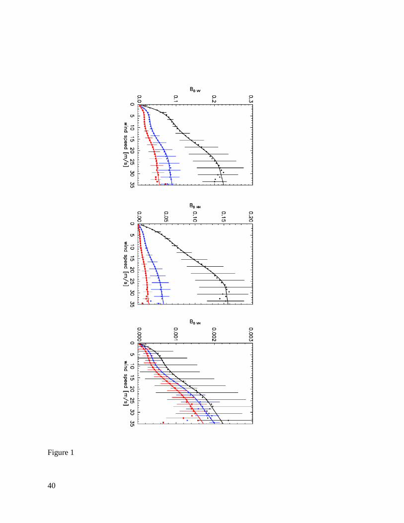
40

Figure 1

41

Figure 2

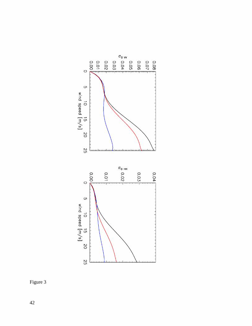
42

Figure 3

43

Figure 4

44

Figure 5

45

Figure 6

46

Figure 7

47

Figure 8

48

Figure 9

49

Figure 10

50

Figure 11

51

Figure 12

52

Figure 13

53

Figure 14

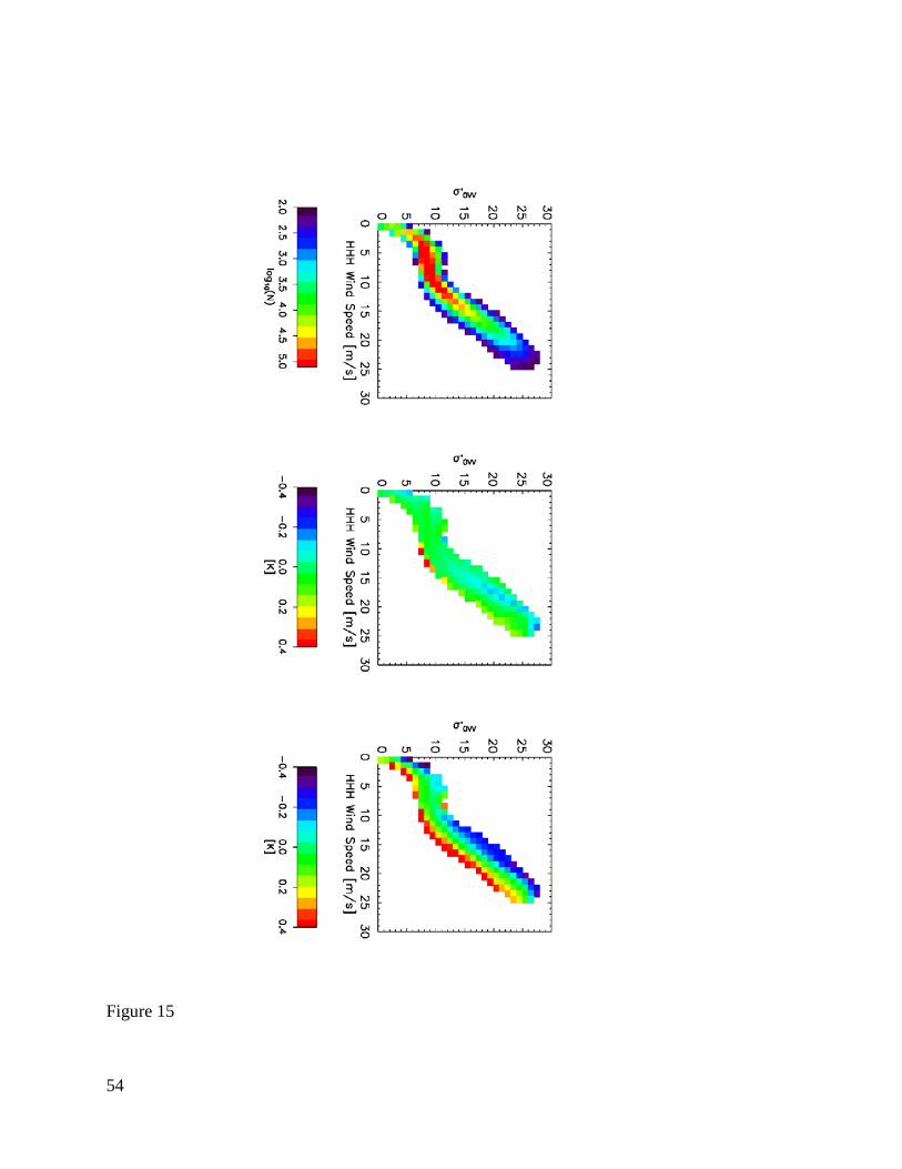
54

Figure 15

55

Figure 16

56

Figure 17

57

Figure 18

58

Auxiliary Material for

A geophysical model for the emission and scattering of L-band microwave radiation from rough ocean surfaces.

Thomas Meissner and Frank J. Wentz

(Remote Sensing Systems, 444 Tenth Street, Suite 200, Santa Rosa, CA 95401, USA)

Journal of Geophysical Research, Oceans, 2014

Introduction

This auxiliary material includes tables containing coefficients for the various geophysical model functions that are used in this publication.

1. ts01.txt: The coefficients bki of the 5th order polynomial fit to the harmonic coefficients of the scatterometer GMF. k=0,1,2 indicates the order of the harmonic and i=1,2,3,4,5 the order of the power in the polynomial. The values are provided for all 3 radiometers and polariza-tions VV, HH, and VH. The value for i=1,2,3,4,5 is the 1st column and the value for bki is the 2nd column.

2. ts02.txt: The coefficients aki of the 5th order polynomial fit to the harmonic coefficients of the wind induced emissivity GMF. k=0,1,2 indicates the order of the harmonic and i=1,2,3,4,5 the order of the power in the polynomial. The values are provided for all 3 radi-ometers and V-pol and H-pol. The value for i=1,2,3,4,5 is the 1st column and the value for aki is the 2nd column.

3. ts03.txt: Expected errors for the channels (scatterometer HH and radiometer H-pol) that are used in the MLE as a function of surface wind speed. The 1st column is the wind speed. The next 3 columns are the expected standard deviations of σ0HH [in real units], TBH [in K] and the NCEP background wind speed WNCEP [in m/s] for radiometer 1, 2 and 3, respectively.

4. ts04.txt: The correction ΔE1 (WHHH, σ’0VV) to the wind induced emissivity. The values are provided for all 3 radiometers and polarizations V-pol and H-pol. The 1st column is the HHH wind speed WHHH [in m/s], the 2nd column is the scatterometer VV-pol cross section σ’0VV af-ter removing the wind direction signal [in real units], the 3rd column is the number of obser-vation in each interval, and the last column the value of ΔE1 [multiplied by 290 K]. Intervals with less than 100 observations are not listed.

5. ts05.txt: The correction ΔE2 (WHHH, WH) to the wind induced emissivity. The values are provided for all 3 radiometers and polarizations V-pol and H-pol. The 1st column is the HHH wind speed WHHH [in m/s], the 2nd column is the significant wave height WH [in m], the 3rd column is the number of observation in each interval, and the last column the value of ΔE2 [multiplied by 290 K]. Intervals with less than 100 observations are not listed.

59

ts01.txt

radiometer 1 VV b 0i 1 2.7669953402e-002 2 -3.5648121980e-003 3 2.5085738933e-004 4 -7.6604470290e-006 5 8.3403936421e-008 radiometer 1 VV b 1i 1 3.1471932686e-004 2 -1.0708873066e-004 3 9.8366727292e-006 4 -1.5828345752e-007 5 -2.3597221602e-009 radiometer 1 VV b 2i 1 1.9129701422e-003 2 -1.4546678790e-003 3 2.1484907649e-004 4 -9.9712358461e-006 5 1.5136841055e-007 radiometer 1 HH b 0i 1 1.2755914080e-002 2 -1.1566306028e-003 3 7.5880134855e-005 4 -2.1193397012e-006 5 1.9732074898e-008 radiometer 1 HH b 1i 1 3.6370936768e-004 2 -1.1753728728e-004 3 1.3593095709e-005 4 -3.4977915542e-007 5 8.1882224455e-010 radiometer 1 HH b 2i 1 1.5807451212e-003 2 -9.5377945712e-004 3 1.3424379381e-004

60

4 -6.0496459000e-006 5 8.9841023600e-008 radiometer 1 VH b 0i 1 1.9041911638e-004 2 -2.4137499915e-005 3 1.6633064884e-006 4 -4.5692164746e-008 5 4.1017449367e-010 radiometer 1 VH b 1i 1 -2.5270345066e-005 2 1.9095363812e-005 3 -2.7666404448e-006 4 1.3956850131e-007 5 -2.3159389660e-009 radiometer 1 VH b 2i 1 -3.0904528219e-005 2 6.9945782218e-006 3 -4.5969356549e-007 4 1.4793445441e-008 5 -2.0473917589e-010 radiometer 2 VV b 0i 1 1.2863352200e-002 2 -2.0993592491e-003 3 1.6518875147e-004 4 -5.4682006056e-006 5 6.4132838313e-008 radiometer 2 VV b 1i 1 5.2348832960e-004 2 -2.0409803674e-004 3 2.6073582526e-005 4 -1.1566411871e-006 5 1.7537140274e-008 radiometer 2 VV b 2i 1 5.5889743658e-004 2 -5.0187584565e-004 3 7.9280278992e-005

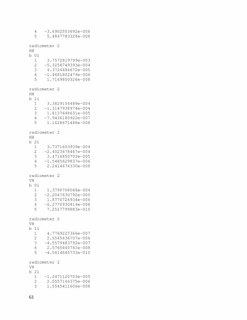
61

4 -3.6902553692e-006 5 5.4847783328e-008 radiometer 2 HH b 0i 1 3.7572819799e-003 2 -5.3258749393e-004 3 4.3724484672e-005 4 -1.4681802479e-006 5 1.7169850326e-008 radiometer 2 HH b 1i 1 3.3829156489e-004 2 -1.3147938974e-004 3 1.8137648631e-005 4 -7.9436180922e-007 5 1.1628671488e-008 radiometer 2 HH b 2i 1 3.7371603939e-004 2 -2.4023678467e-004 3 3.4716850703e-005 4 -1.5485629837e-006 5 2.2414676330e-008 radiometer 2 VH b 0i 1 1.3790708068e-004 2 -2.2047630792e-005 3 1.8770726934e-006 4 -6.2770930814e-008 5 7.2517799883e-010 radiometer 2 VH b 1i 1 4.7769227366e-007 2 2.5545436707e-006 3 -4.5579483792e-007 4 2.5765445741e-008 5 -4.5614845733e-010 radiometer 2 VH b 2i 1 -1.2471120703e-005 2 2.0557144375e-006 3 1.5545411606e-008

62

4 -5.1412937047e-009 5 1.0030170313e-010 radiometer 3 VV b 0i 1 7.9812841854e-003 2 -1.4250014823e-003 3 1.1846924116e-004 4 -4.0865529161e-006 5 4.9691503580e-008 radiometer 3 VV b 1i 1 2.8558723483e-004 2 -1.1332749701e-004 3 1.4903721848e-005 4 -6.4922700321e-007 5 9.4205608577e-009 radiometer 3 VV b 2i 1 4.4372478525e-004 2 -3.1164511936e-004 3 4.9980678917e-005 4 -2.3909290707e-006 5 3.6603560390e-008 radiometer 3 HH b 0i 1 1.4664950940e-003 2 -2.4374331007e-004 3 2.1823161004e-005 4 -7.7367920090e-007 5 9.4709584062e-009 radiometer 3 HH b 1i 1 1.2856275234e-004 2 -5.0136994111e-005 3 7.3669264038e-006 4 -3.1710126109e-007 5 4.4180628101e-009 radiometer 3 HH b 2i 1 1.5707164701e-004 2 -9.3649029302e-005 3 1.3860196514e-005

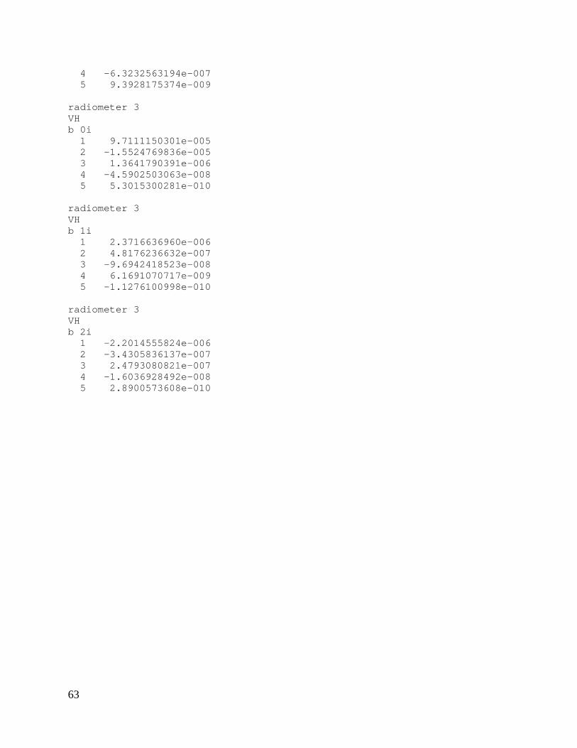
63

4 -6.3232563194e-007 5 9.3928175374e-009 radiometer 3 VH b 0i 1 9.7111150301e-005 2 -1.5524769836e-005 3 1.3641790391e-006 4 -4.5902503063e-008 5 5.3015300281e-010 radiometer 3 VH b 1i 1 2.3716636960e-006 2 4.8176236632e-007 3 -9.6942418523e-008 4 6.1691070717e-009 5 -1.1276100998e-010 radiometer 3 VH b 2i 1 -2.2014555824e-006 2 -3.4305836137e-007 3 2.4793080821e-007 4 -1.6036928492e-008 5 2.8900573608e-010

64

ts02.txt

radiometer 1 V a 0i 1 5.7894060320e-001 2 -1.0473595790e-001 3 9.9200140518e-003 4 -3.6291757411e-004 5 4.6589912401e-006 radiometer 1 V a 1i 1 2.1216534279e-002 2 -7.1813519762e-003 3 9.1738225933e-004 4 -3.9535822500e-005 5 5.6502242949e-007 radiometer 1 V a 2i 1 6.6222103677e-002 2 -2.8388133825e-002 3 3.7501350060e-003 4 -1.8446699362e-004 5 3.1286830745e-006 radiometer 1 H a 0i 1 7.7153019419e-001 2 -1.2715188465e-001 3 1.1329089683e-002 4 -4.0789149957e-004 5 5.2183370672e-006 radiometer 1 H a 1i 1 3.3306056615e-003 2 -3.7204789320e-003 3 6.2494297864e-004 4 -3.2678064089e-005 5 5.3603866560e-007 radiometer 1 H a 2i 1 -1.2192070798e-002 2 8.8557322073e-003 3 -1.2734161054e-003

65

4 5.1704466145e-005 5 -5.8171521631e-007 radiometer 2 V a 0i 1 5.0281588143e-001 2 -8.4035755450e-002 3 7.8518455026e-003 4 -2.8030380618e-004 5 3.5109805876e-006 radiometer 2 V a 1i 1 1.5596703582e-003 2 2.3582984624e-003 3 -3.4662668911e-004 4 2.6606348124e-005 5 -6.1842609629e-007 radiometer 2 V a 2i 1 5.1196349082e-002 2 -1.8202980254e-002 3 2.0749477038e-003 4 -8.6995183107e-005 5 1.2436524520e-006 radiometer 2 H a 0i 1 8.4965177001e-001 2 -1.2443856200e-001 3 1.0359930394e-002 4 -3.5549109274e-004 5 4.3636667626e-006 radiometer 2 H a 1i 1 -1.8863269506e-002 2 6.5676785996e-003 3 -7.3111819961e-004 4 3.7255111733e-005 5 -6.8989289663e-007 radiometer 2 H a 2i 1 -4.8938315835e-002 2 2.6541378947e-002 3 -3.7836135549e-003

66

4 1.9204055354e-004 5 -3.2620602022e-006 radiometer 3 V a 0i 1 4.7027203005e-001 2 -7.6334662983e-002 3 6.9857495929e-003 4 -2.4303426684e-004 5 2.9390853226e-006 radiometer 3 V a 1i 1 9.1197181127e-003 2 -3.0431623312e-003 3 5.0839571367e-004 4 -2.0375986729e-005 5 2.4580823525e-007 radiometer 3 V a 2i 1 9.3408423686e-002 2 -3.3492931571e-002 3 3.8025601997e-003 4 -1.6925890570e-004 5 2.6396519557e-006 radiometer 3 H a 0i 1 1.0601673642e+000 2 -1.4677107298e-001 3 1.1480019211e-002 4 -3.8084012081e-004 5 4.5485097434e-006 radiometer 3 H a 1i 1 9.6160121528e-003 2 -4.3505334225e-003 3 6.0718079191e-004 4 -2.7536464802e-005 5 4.0733177632e-007 radiometer 3 H a 2i 1 -5.1974877527e-003 2 1.0855313411e-002 3 -1.8411735248e-003

67

4 9.5714130699e-005 5 -1.6059448322e-006

68

ts03.txt

Wind speedsigma0 HH TB H W NCEP sigma0 HH TB H W NCEP sigma0 HH TB H W NCEP

0 0.002162 0.204694 1.118146 0.000478 0.196523 1.118146 0.000222 0.218601 1.1181461 0.002811 0.216598 1.035427 0.000657 0.227773 1.035427 0.000253 0.244698 1.0354272 0.003554 0.237533 0.941831 0.000837 0.260301 0.941831 0.000324 0.281098 0.9418313 0.003397 0.244513 0.942946 0.000803 0.255531 0.942946 0.000319 0.281507 0.9429464 0.003128 0.241825 0.961688 0.000755 0.244097 0.961688 0.000273 0.265312 0.9616885 0.003005 0.237435 0.967645 0.000692 0.233588 0.967645 0.000257 0.253008 0.9676456 0.002742 0.232175 0.965748 0.000605 0.223152 0.965748 0.000247 0.241897 0.9657487 0.002561 0.232554 0.966377 0.000561 0.21475 0.966377 0.000251 0.232883 0.9663778 0.002669 0.238376 0.982044 0.000589 0.214677 0.982044 0.000252 0.230973 0.9820449 0.003058 0.243367 1.036862 0.000661 0.223211 1.036862 0.000284 0.241124 1.036862

10 0.003575 0.246757 1.121006 0.000768 0.235413 1.121006 0.000364 0.259865 1.12100611 0.004267 0.264352 1.2319 0.000999 0.257846 1.2319 0.000474 0.286123 1.231912 0.005234 0.292643 1.344265 0.001326 0.291839 1.344265 0.000663 0.316673 1.34426513 0.006088 0.316431 1.407236 0.001615 0.321048 1.407236 0.000803 0.339212 1.40723614 0.006793 0.336506 1.427256 0.001938 0.336179 1.427256 0.000874 0.353528 1.42725615 0.007678 0.361546 1.449059 0.002158 0.352008 1.449059 0.001027 0.377721 1.44905916 0.008665 0.38954 1.527995 0.002431 0.393054 1.527995 0.001215 0.419884 1.52799517 0.009586 0.416811 1.583605 0.002833 0.444346 1.583605 0.001321 0.467506 1.58360518 0.010366 0.455024 1.64357 0.003222 0.483129 1.64357 0.001476 0.495254 1.6435719 0.011534 0.489119 1.840392 0.003846 0.5 1.840392 0.001586 0.5 1.84039220 0.012506 0.5 2.07388 0.003906 0.5 2.07388 0.001705 0.5 2.0738821 0.013046 0.5 2.328262 0.003823 0.5 2.328262 0.001769 0.5 2.32826222 0.013826 0.5 2.637159 0.004314 0.5 2.637159 0.0016 0.5 2.63715923 0.014606 0.5 2.946057 0.004805 0.5 2.946057 0.001431 0.5 2.94605724 0.015386 0.5 3.254955 0.005297 0.5 3.254955 0.001262 0.5 3.25495525 0.016166 0.5 3.563852 0.005788 0.5 3.563852 0.001094 0.5 3.563852

Radiometer 1 Radiometer 2 Radiometer 3

69

ts04.txt

radiometer 1 V 0.5 0.0040 10229 0.0040 0.5 0.0120 15912 -0.0049 0.5 0.0200 13403 -0.0292 0.5 0.0280 3965 -0.0574 0.5 0.0360 292 -0.0567 1.5 0.0120 1045 0.1917 1.5 0.0200 8447 0.0422 1.5 0.0280 23236 -0.0055 1.5 0.0360 30708 -0.0282 1.5 0.0440 18143 -0.0519 1.5 0.0520 3553 -0.0638 1.5 0.0600 163 -0.0712 2.5 0.0280 162 0.8728 2.5 0.0360 3571 0.1038 2.5 0.0440 25586 -0.0011 2.5 0.0520 52715 -0.0298 2.5 0.0600 38559 -0.0265 2.5 0.0680 3244 -0.0332 3.5 0.0440 114 0.6997 3.5 0.0520 5147 0.0434 3.5 0.0600 66566 0.0051 3.5 0.0680 117641 0.0068 3.5 0.0760 13183 -0.0132 3.5 0.0840 363 0.0133 4.5 0.0600 2566 0.0942 4.5 0.0680 117475 0.0218 4.5 0.0760 181912 0.0067 4.5 0.0840 23573 -0.0138 4.5 0.0920 1426 0.0165 5.5 0.0680 9084 0.0769 5.5 0.0760 255013 0.0147 5.5 0.0840 163786 -0.0094 5.5 0.0920 26611 -0.0151 5.5 0.1000 1128 0.0319 6.5 0.0680 284 0.4528 6.5 0.0760 47586 0.0516 6.5 0.0840 401153 0.0090 6.5 0.0920 107114 -0.0218 6.5 0.1000 8804 -0.0148 6.5 0.1080 186 -0.0664 7.5 0.0760 2694 0.1210 7.5 0.0840 195813 0.0366

70

7.5 0.0920 368850 0.0059 7.5 0.1000 28063 -0.0492 7.5 0.1080 960 -0.1195 7.5 0.1160 117 -0.2181 8.5 0.0760 143 0.3551 8.5 0.0840 22244 0.0956 8.5 0.0920 370929 0.0276 8.5 0.1000 137197 -0.0021 8.5 0.1080 3190 -0.1954 8.5 0.1160 456 -0.1821 9.5 0.0840 2365 0.1300 9.5 0.0920 93385 0.0497 9.5 0.1000 297331 0.0140 9.5 0.1080 31280 -0.0213 9.5 0.1160 1331 -0.2402 9.5 0.1240 277 -0.2669 10.5 0.0840 196 0.2080 10.5 0.0920 12724 0.0602 10.5 0.1000 143421 0.0144 10.5 0.1080 148377 0.0005 10.5 0.1160 9419 -0.0241 10.5 0.1240 626 -0.1950 10.5 0.1320 172 -0.2918 11.5 0.0920 1318 0.0827 11.5 0.1000 28781 0.0056 11.5 0.1080 124940 -0.0128 11.5 0.1160 75412 -0.0026 11.5 0.1240 4930 -0.0056 11.5 0.1320 471 -0.1132 11.5 0.1400 131 -0.1285 12.5 0.0920 213 0.1929 12.5 0.1000 3758 -0.0047 12.5 0.1080 35094 -0.0378 12.5 0.1160 88575 -0.0327 12.5 0.1240 45176 -0.0183 12.5 0.1320 4269 0.0054 12.5 0.1400 484 0.0240 12.5 0.1480 140 0.1246 13.5 0.1000 509 0.0009 13.5 0.1080 4869 -0.0565 13.5 0.1160 30330 -0.0682 13.5 0.1240 59861 -0.0609 13.5 0.1320 31760 -0.0447 13.5 0.1400 4774 -0.0139 13.5 0.1480 604 0.0817 13.5 0.1560 175 0.1220 14.5 0.1000 131 -0.0217

71

14.5 0.1080 651 -0.0583 14.5 0.1160 4446 -0.0932 14.5 0.1240 20554 -0.1014 14.5 0.1320 38038 -0.0852 14.5 0.1400 24197 -0.0616 14.5 0.1480 5144 -0.0345 14.5 0.1560 766 0.0268 14.5 0.1640 215 0.0989 15.5 0.1080 194 0.1461 15.5 0.1160 550 -0.0181 15.5 0.1240 2942 -0.1073 15.5 0.1320 13537 -0.1077 15.5 0.1400 24828 -0.1047 15.5 0.1480 17890 -0.0941 15.5 0.1560 5035 -0.0606 15.5 0.1640 947 0.0091 15.5 0.1720 268 0.0863 15.5 0.1800 117 0.1320 16.5 0.1160 154 0.0301 16.5 0.1240 520 -0.0560 16.5 0.1320 2365 -0.1073 16.5 0.1400 8451 -0.1184 16.5 0.1480 15088 -0.1139 16.5 0.1560 12509 -0.1043 16.5 0.1640 4611 -0.0822 16.5 0.1720 1018 -0.0293 16.5 0.1800 272 0.0479 17.5 0.1240 126 -0.0248 17.5 0.1320 382 -0.0384 17.5 0.1400 1359 -0.0659 17.5 0.1480 4988 -0.0952 17.5 0.1560 8956 -0.1028 17.5 0.1640 7895 -0.1081 17.5 0.1720 3576 -0.0904 17.5 0.1800 979 -0.0240 17.5 0.1880 276 0.0649 17.5 0.1960 128 0.0966 18.5 0.1320 115 0.0642 18.5 0.1400 239 -0.0742 18.5 0.1480 970 -0.0388 18.5 0.1560 2837 -0.0409 18.5 0.1640 5114 -0.0814 18.5 0.1720 5083 -0.0891 18.5 0.1800 2822 -0.0953 18.5 0.1880 927 -0.0424 18.5 0.1960 288 -0.0019 18.5 0.2040 116 0.1495 19.5 0.1480 190 0.0910 19.5 0.1560 607 -0.0046

72

19.5 0.1640 1772 -0.0233 19.5 0.1720 2704 -0.0299 19.5 0.1800 2936 -0.0606 19.5 0.1880 2050 -0.0844 19.5 0.1960 886 -0.0483 19.5 0.2040 251 0.0143 20.5 0.1560 139 0.0551 20.5 0.1640 400 0.0616 20.5 0.1720 946 0.0717 20.5 0.1800 1416 0.0130 20.5 0.1880 1558 -0.0229 20.5 0.1960 1376 -0.0608 20.5 0.2040 658 -0.0552 21.5 0.1640 104 0.1418 21.5 0.1720 311 0.0881 21.5 0.1800 619 0.0739 21.5 0.1880 920 0.0751 21.5 0.1960 940 0.0376 21.5 0.2040 657 0.0172 22.5 0.1720 114 0.1164 22.5 0.1800 226 0.1316 22.5 0.1880 317 0.1181 22.5 0.1960 453 0.0921 22.5 0.2040 477 0.0927 23.5 0.1880 174 0.1593 23.5 0.1960 207 0.1245 23.5 0.2040 287 0.1823 24.5 0.1960 133 0.1494 24.5 0.2040 176 0.1943 25.5 0.1960 112 0.2196 25.5 0.2040 112 0.2847 radiometer 1 H 0.5 0.0040 10229 0.1111 0.5 0.0120 15912 0.0701 0.5 0.0200 13403 -0.0279 0.5 0.0280 3965 -0.2038 0.5 0.0360 292 -0.4010 1.5 0.0120 1045 0.4792 1.5 0.0200 8447 0.2326 1.5 0.0280 23236 0.0823 1.5 0.0360 30708 -0.0156 1.5 0.0440 18143 -0.1487 1.5 0.0520 3553 -0.3431 1.5 0.0600 163 -0.5406

73

2.5 0.0280 162 1.0679 2.5 0.0360 3571 0.3179 2.5 0.0440 25586 0.0895 2.5 0.0520 52715 -0.0316 2.5 0.0600 38559 -0.1350 2.5 0.0680 3244 -0.2560 3.5 0.0440 114 1.0214 3.5 0.0520 5147 0.1810 3.5 0.0600 66566 0.0312 3.5 0.0680 117641 -0.0319 3.5 0.0760 13183 -0.0895 3.5 0.0840 363 -0.1502 4.5 0.0600 2566 0.2171 4.5 0.0680 117475 0.0619 4.5 0.0760 181912 -0.0044 4.5 0.0840 23573 -0.0816 4.5 0.0920 1426 -0.0944 5.5 0.0680 9084 0.1822 5.5 0.0760 255013 0.0495 5.5 0.0840 163786 -0.0401 5.5 0.0920 26611 -0.1085 5.5 0.1000 1128 -0.1017 6.5 0.0680 284 0.7073 6.5 0.0760 47586 0.1135 6.5 0.0840 401153 0.0134 6.5 0.0920 107114 -0.0877 6.5 0.1000 8804 -0.1140 6.5 0.1080 186 -0.1105 7.5 0.0760 2694 0.1950 7.5 0.0840 195813 0.0645 7.5 0.0920 368850 -0.0199 7.5 0.1000 28063 -0.1247 7.5 0.1080 960 -0.1461 7.5 0.1160 117 -0.1363 8.5 0.0760 143 0.4716 8.5 0.0840 22244 0.1540 8.5 0.0920 370929 0.0327 8.5 0.1000 137197 -0.0614 8.5 0.1080 3190 -0.2427 8.5 0.1160 456 -0.1669 9.5 0.0840 2365 0.2028 9.5 0.0920 93385 0.1054 9.5 0.1000 297331 0.0007 9.5 0.1080 31280 -0.1349 9.5 0.1160 1331 -0.2978 9.5 0.1240 277 -0.3318

74

10.5 0.0840 196 0.3752 10.5 0.0920 12724 0.1592 10.5 0.1000 143421 0.0649 10.5 0.1080 148377 -0.0437 10.5 0.1160 9419 -0.1831 10.5 0.1240 626 -0.2895 10.5 0.1320 172 -0.3823 11.5 0.0920 1318 0.2875 11.5 0.1000 28781 0.1161 11.5 0.1080 124940 0.0276 11.5 0.1160 75412 -0.0829 11.5 0.1240 4930 -0.2067 11.5 0.1320 471 -0.2945 11.5 0.1400 131 -0.3131 12.5 0.0920 213 0.7051 12.5 0.1000 3758 0.2165 12.5 0.1080 35094 0.0760 12.5 0.1160 88575 -0.0058 12.5 0.1240 45176 -0.1136 12.5 0.1320 4269 -0.2198 12.5 0.1400 484 -0.2546 12.5 0.1480 140 -0.2441 13.5 0.1000 509 0.5187 13.5 0.1080 4869 0.1780 13.5 0.1160 30330 0.0528 13.5 0.1240 59861 -0.0349 13.5 0.1320 31760 -0.1424 13.5 0.1400 4774 -0.2352 13.5 0.1480 604 -0.2673 13.5 0.1560 175 -0.2654 14.5 0.1000 131 0.9524 14.5 0.1080 651 0.3649 14.5 0.1160 4446 0.1461 14.5 0.1240 20554 0.0284 14.5 0.1320 38038 -0.0559 14.5 0.1400 24197 -0.1610 14.5 0.1480 5144 -0.2479 14.5 0.1560 766 -0.2922 14.5 0.1640 215 -0.3405 15.5 0.1080 194 0.7996 15.5 0.1160 550 0.4248 15.5 0.1240 2942 0.1314 15.5 0.1320 13537 0.0236 15.5 0.1400 24828 -0.0689 15.5 0.1480 17890 -0.1733 15.5 0.1560 5035 -0.2564 15.5 0.1640 947 -0.2959 15.5 0.1720 268 -0.3187

75

15.5 0.1800 117 -0.3155 16.5 0.1160 154 0.8530 16.5 0.1240 520 0.3965 16.5 0.1320 2365 0.1563 16.5 0.1400 8451 0.0261 16.5 0.1480 15088 -0.0632 16.5 0.1560 12509 -0.1681 16.5 0.1640 4611 -0.2538 16.5 0.1720 1018 -0.2975 16.5 0.1800 272 -0.3197 17.5 0.1240 126 0.6882 17.5 0.1320 382 0.3837 17.5 0.1400 1359 0.2032 17.5 0.1480 4988 0.0598 17.5 0.1560 8956 -0.0550 17.5 0.1640 7895 -0.1661 17.5 0.1720 3576 -0.2483 17.5 0.1800 979 -0.3052 17.5 0.1880 276 -0.3167 17.5 0.1960 128 -0.3449 18.5 0.1320 115 0.6936 18.5 0.1400 239 0.3662 18.5 0.1480 970 0.2053 18.5 0.1560 2837 0.0866 18.5 0.1640 5114 -0.0374 18.5 0.1720 5083 -0.1528 18.5 0.1800 2822 -0.2408 18.5 0.1880 927 -0.3062 18.5 0.1960 288 -0.3596 18.5 0.2040 116 -0.2853 19.5 0.1480 190 0.4465 19.5 0.1560 607 0.2389 19.5 0.1640 1772 0.1324 19.5 0.1720 2704 0.0180 19.5 0.1800 2936 -0.1173 19.5 0.1880 2050 -0.2323 19.5 0.1960 886 -0.3061 19.5 0.2040 251 -0.3482 20.5 0.1560 139 0.4720 20.5 0.1640 400 0.3250 20.5 0.1720 946 0.1999 20.5 0.1800 1416 0.0518 20.5 0.1880 1558 -0.0893 20.5 0.1960 1376 -0.2048 20.5 0.2040 658 -0.2982 21.5 0.1640 104 0.4780 21.5 0.1720 311 0.2993 21.5 0.1800 619 0.1892

76

21.5 0.1880 920 0.0825 21.5 0.1960 940 -0.0306 21.5 0.2040 657 -0.1415 22.5 0.1720 114 0.3796 22.5 0.1800 226 0.2459 22.5 0.1880 317 0.1783 22.5 0.1960 453 0.0833 22.5 0.2040 477 -0.0006 23.5 0.1880 174 0.2517 23.5 0.1960 207 0.1884 23.5 0.2040 287 0.1270 24.5 0.1960 133 0.2270 24.5 0.2040 176 0.1879 25.5 0.1960 112 0.2787 25.5 0.2040 112 0.3255 radiometer 2 V 0.5 0.0015 5083 0.0035 0.5 0.0045 10076 -0.0099 0.5 0.0075 13070 -0.0232 0.5 0.0105 9939 -0.0564 0.5 0.0135 2831 -0.0928 0.5 0.0165 277 -0.0989 1.5 0.0075 1114 0.1214 1.5 0.0105 8314 0.0202 1.5 0.0135 20723 -0.0183 1.5 0.0165 26790 -0.0398 1.5 0.0195 17053 -0.0521 1.5 0.0225 4759 -0.0528 1.5 0.0255 473 -0.0260 2.5 0.0135 198 0.3024 2.5 0.0165 4356 0.0565 2.5 0.0195 25186 -0.0137 2.5 0.0225 49631 -0.0247 2.5 0.0255 36388 -0.0056 2.5 0.0285 4502 0.0117 2.5 0.0315 109 -0.0602 3.5 0.0195 580 0.1899 3.5 0.0225 14804 0.0182 3.5 0.0255 90785 0.0031 3.5 0.0285 77501 0.0241 3.5 0.0315 7043 -0.0251 3.5 0.0345 373 -0.0361 4.5 0.0225 831 0.1755

77

4.5 0.0255 51477 0.0175 4.5 0.0285 193427 0.0255 4.5 0.0315 44997 -0.0003 4.5 0.0345 9978 -0.0197 4.5 0.0375 1067 0.0249 5.5 0.0255 17610 0.0509 5.5 0.0285 253933 0.0153 5.5 0.0315 121550 0.0104 5.5 0.0345 29496 -0.0172 5.5 0.0375 6096 0.0125 5.5 0.0405 287 0.0238 6.5 0.0255 3407 0.0826 6.5 0.0285 201581 0.0179 6.5 0.0315 269114 0.0023 6.5 0.0345 43735 -0.0202 6.5 0.0375 9717 -0.0058 6.5 0.0405 247 0.0474 7.5 0.0255 332 0.3060 7.5 0.0285 84315 0.0179 7.5 0.0315 399066 0.0059 7.5 0.0345 63761 -0.0155 7.5 0.0375 7315 0.0005 7.5 0.0405 228 -0.0619 8.5 0.0285 16237 0.0405 8.5 0.0315 303747 0.0164 8.5 0.0345 172718 -0.0038 8.5 0.0375 5340 -0.0215 8.5 0.0405 252 -0.1632 9.5 0.0285 1374 0.0701 9.5 0.0315 96913 0.0139 9.5 0.0345 262263 0.0056 9.5 0.0375 37503 -0.0003 9.5 0.0405 547 -0.0979 10.5 0.0285 184 0.1746 10.5 0.0315 11902 0.0230 10.5 0.0345 131693 -0.0010 10.5 0.0375 136883 -0.0026 10.5 0.0405 13539 0.0099 10.5 0.0435 273 -0.0732 11.5 0.0315 1283 0.1083 11.5 0.0345 21961 -0.0058 11.5 0.0375 105805 -0.0161 11.5 0.0405 80552 -0.0124 11.5 0.0435 10234 0.0077 11.5 0.0465 419 0.0205 12.5 0.0315 246 0.0770

78

12.5 0.0345 2168 0.0190 12.5 0.0375 20764 -0.0246 12.5 0.0405 71753 -0.0315 12.5 0.0435 56197 -0.0256 12.5 0.0465 11769 -0.0043 12.5 0.0495 957 0.0400 12.5 0.0525 112 -0.0267 13.5 0.0345 367 0.0721 13.5 0.0375 2182 -0.0091 13.5 0.0405 14279 -0.0402 13.5 0.0435 44631 -0.0459 13.5 0.0465 43776 -0.0416 13.5 0.0495 14577 -0.0220 13.5 0.0525 2046 0.0174 13.5 0.0555 245 0.0478 14.5 0.0345 116 0.1895 14.5 0.0375 369 0.1049 14.5 0.0405 1961 -0.0198 14.5 0.0435 8934 -0.0506 14.5 0.0465 25458 -0.0577 14.5 0.0495 31216 -0.0664 14.5 0.0525 15406 -0.0513 14.5 0.0555 3922 -0.0141 14.5 0.0585 547 0.0118 14.5 0.0615 127 0.0141 15.5 0.0405 356 0.1788 15.5 0.0435 1236 -0.0506 15.5 0.0465 4839 -0.0472 15.5 0.0495 13449 -0.0770 15.5 0.0525 21014 -0.0880 15.5 0.0555 14173 -0.0817 15.5 0.0585 5086 -0.0524 15.5 0.0615 1164 -0.0137 15.5 0.0645 268 0.0007 16.5 0.0435 230 0.0125 16.5 0.0465 687 -0.0374 16.5 0.0495 2314 -0.0487 16.5 0.0525 6939 -0.0836 16.5 0.0555 12433 -0.0879 16.5 0.0585 10938 -0.0950 16.5 0.0615 5648 -0.0957 16.5 0.0645 1851 -0.0521 16.5 0.0675 445 0.0027 16.5 0.0705 139 -0.0186 17.5 0.0465 136 0.1819 17.5 0.0495 348 0.0403 17.5 0.0525 1240 -0.0288 17.5 0.0555 3412 -0.0470 17.5 0.0585 6627 -0.0711

79

17.5 0.0615 7374 -0.0834 17.5 0.0645 5009 -0.1066 17.5 0.0675 2460 -0.0846 17.5 0.0705 725 -0.0259 17.5 0.0735 169 0.0269 18.5 0.0525 264 0.0491 18.5 0.0555 742 -0.0034 18.5 0.0585 1742 -0.0290 18.5 0.0615 3475 -0.0458 18.5 0.0645 4155 -0.0612 18.5 0.0675 3393 -0.0836 18.5 0.0705 2223 -0.0932 18.5 0.0735 826 -0.0952 18.5 0.0765 258 -0.0423 19.5 0.0555 183 0.1712 19.5 0.0585 370 0.0541 19.5 0.0615 889 0.0248 19.5 0.0645 1880 -0.0108 19.5 0.0675 2346 -0.0238 19.5 0.0705 1818 -0.0240 19.5 0.0735 1559 -0.0528 19.5 0.0765 896 -0.0897 20.5 0.0585 111 0.0856 20.5 0.0615 257 0.1352 20.5 0.0645 495 0.0452 20.5 0.0675 1074 0.0181 20.5 0.0705 1287 0.0146 20.5 0.0735 1154 0.0600 20.5 0.0765 778 0.0088 21.5 0.0645 210 0.1477 21.5 0.0675 301 0.0754 21.5 0.0705 547 0.0389 21.5 0.0735 731 0.0385 21.5 0.0765 457 0.0567 22.5 0.0675 109 0.1743 22.5 0.0705 199 0.0995 22.5 0.0735 372 0.0352 22.5 0.0765 357 0.0956 23.5 0.0705 109 0.0602 23.5 0.0735 178 0.0320 23.5 0.0765 247 0.1306 24.5 0.0765 173 0.0686 radiometer 2 H

80

0.5 0.0015 5083 0.1038 0.5 0.0045 10076 0.0920 0.5 0.0075 13070 0.0616 0.5 0.0105 9939 -0.0563 0.5 0.0135 2831 -0.2580 0.5 0.0165 277 -0.4856 1.5 0.0075 1114 0.4415 1.5 0.0105 8314 0.2246 1.5 0.0135 20723 0.0872 1.5 0.0165 26790 -0.0069 1.5 0.0195 17053 -0.1428 1.5 0.0225 4759 -0.3089 1.5 0.0255 473 -0.4691 2.5 0.0135 198 0.6012 2.5 0.0165 4356 0.2755 2.5 0.0195 25186 0.0939 2.5 0.0225 49631 -0.0264 2.5 0.0255 36388 -0.1302 2.5 0.0285 4502 -0.2280 2.5 0.0315 109 -0.4485 3.5 0.0195 580 0.3883 3.5 0.0225 14804 0.1399 3.5 0.0255 90785 0.0182 3.5 0.0285 77501 -0.0441 3.5 0.0315 7043 -0.1072 3.5 0.0345 373 -0.1750 4.5 0.0225 831 0.3191 4.5 0.0255 51477 0.0967 4.5 0.0285 193427 0.0243 4.5 0.0315 44997 -0.0470 4.5 0.0345 9978 -0.1122 4.5 0.0375 1067 -0.1012 5.5 0.0255 17610 0.1529 5.5 0.0285 253933 0.0503 5.5 0.0315 121550 -0.0131 5.5 0.0345 29496 -0.0907 5.5 0.0375 6096 -0.1005 5.5 0.0405 287 -0.1029 6.5 0.0255 3407 0.1892 6.5 0.0285 201581 0.0660 6.5 0.0315 269114 -0.0040 6.5 0.0345 43735 -0.0847 6.5 0.0375 9717 -0.0863 6.5 0.0405 247 -0.0516 7.5 0.0255 332 0.2990 7.5 0.0285 84315 0.0778 7.5 0.0315 399066 0.0078

81

7.5 0.0345 63761 -0.0679 7.5 0.0375 7315 -0.0477 7.5 0.0405 228 0.1515 8.5 0.0285 16237 0.1104 8.5 0.0315 303747 0.0420 8.5 0.0345 172718 -0.0449 8.5 0.0375 5340 -0.0235 8.5 0.0405 252 0.0852 9.5 0.0285 1374 0.1322 9.5 0.0315 96913 0.0859 9.5 0.0345 262263 -0.0012 9.5 0.0375 37503 -0.1057 9.5 0.0405 547 -0.0551 10.5 0.0285 184 0.2742 10.5 0.0315 11902 0.1412 10.5 0.0345 131693 0.0541 10.5 0.0375 136883 -0.0456 10.5 0.0405 13539 -0.1634 10.5 0.0435 273 -0.1284 11.5 0.0315 1283 0.3211 11.5 0.0345 21961 0.1211 11.5 0.0375 105805 0.0295 11.5 0.0405 80552 -0.0713 11.5 0.0435 10234 -0.1855 11.5 0.0465 419 -0.1975 12.5 0.0315 246 0.4798 12.5 0.0345 2168 0.2805 12.5 0.0375 20764 0.1056 12.5 0.0405 71753 0.0149 12.5 0.0435 56197 -0.0815 12.5 0.0465 11769 -0.1855 12.5 0.0495 957 -0.2420 12.5 0.0525 112 -0.3055 13.5 0.0345 367 0.4629 13.5 0.0375 2182 0.2561 13.5 0.0405 14279 0.1094 13.5 0.0435 44631 0.0148 13.5 0.0465 43776 -0.0727 13.5 0.0495 14577 -0.1762 13.5 0.0525 2046 -0.2487 13.5 0.0555 245 -0.3011 14.5 0.0345 116 0.6925 14.5 0.0375 369 0.4685 14.5 0.0405 1961 0.2542 14.5 0.0435 8934 0.1268 14.5 0.0465 25458 0.0236 14.5 0.0495 31216 -0.0679

82

14.5 0.0525 15406 -0.1599 14.5 0.0555 3922 -0.2311 14.5 0.0585 547 -0.3101 14.5 0.0615 127 -0.3824 15.5 0.0405 356 0.5661 15.5 0.0435 1236 0.2889 15.5 0.0465 4839 0.1599 15.5 0.0495 13449 0.0313 15.5 0.0525 21014 -0.0535 15.5 0.0555 14173 -0.1426 15.5 0.0585 5086 -0.2130 15.5 0.0615 1164 -0.2712 15.5 0.0645 268 -0.3682 16.5 0.0435 230 0.4976 16.5 0.0465 687 0.3313 16.5 0.0495 2314 0.2015 16.5 0.0525 6939 0.0553 16.5 0.0555 12433 -0.0249 16.5 0.0585 10938 -0.1125 16.5 0.0615 5648 -0.2056 16.5 0.0645 1851 -0.2622 16.5 0.0675 445 -0.3001 16.5 0.0705 139 -0.3783 17.5 0.0465 136 0.6271 17.5 0.0495 348 0.4216 17.5 0.0525 1240 0.2549 17.5 0.0555 3412 0.1167 17.5 0.0585 6627 0.0186 17.5 0.0615 7374 -0.0635 17.5 0.0645 5009 -0.1823 17.5 0.0675 2460 -0.2559 17.5 0.0705 725 -0.2990 17.5 0.0735 169 -0.3477 18.5 0.0525 264 0.4403 18.5 0.0555 742 0.2803 18.5 0.0585 1742 0.1623 18.5 0.0615 3475 0.0738 18.5 0.0645 4155 -0.0155 18.5 0.0675 3393 -0.1337 18.5 0.0705 2223 -0.2458 18.5 0.0735 826 -0.3310 18.5 0.0765 258 -0.4020 19.5 0.0555 183 0.5163 19.5 0.0585 370 0.3775 19.5 0.0615 889 0.2305 19.5 0.0645 1880 0.1246 19.5 0.0675 2346 0.0391 19.5 0.0705 1818 -0.0473 19.5 0.0735 1559 -0.1700

83

19.5 0.0765 896 -0.2864 20.5 0.0585 111 0.5161 20.5 0.0615 257 0.4557 20.5 0.0645 495 0.2633 20.5 0.0675 1074 0.1552 20.5 0.0705 1287 0.0941 20.5 0.0735 1154 0.0228 20.5 0.0765 778 -0.0996 21.5 0.0645 210 0.3862 21.5 0.0675 301 0.2897 21.5 0.0705 547 0.1819 21.5 0.0735 731 0.0985 21.5 0.0765 457 0.0295 22.5 0.0675 109 0.4487 22.5 0.0705 199 0.2919 22.5 0.0735 372 0.1718 22.5 0.0765 357 0.1140 23.5 0.0705 109 0.3468 23.5 0.0735 178 0.2189 23.5 0.0765 247 0.1859 24.5 0.0765 173 0.2330 radiometer 3 V 0.5 0.0010 3328 0.0131 0.5 0.0030 8170 -0.0187 0.5 0.0050 12127 -0.0460 0.5 0.0070 9140 -0.0730 0.5 0.0090 2344 -0.1253 0.5 0.0110 259 -0.1434 1.5 0.0050 1914 0.1045 1.5 0.0070 11707 0.0054 1.5 0.0090 26489 -0.0321 1.5 0.0110 27658 -0.0516 1.5 0.0130 12384 -0.0601 1.5 0.0150 2350 -0.0481 1.5 0.0170 123 -0.0924 2.5 0.0090 1658 0.0632 2.5 0.0110 17779 -0.0051 2.5 0.0130 50967 -0.0264 2.5 0.0150 47312 -0.0107 2.5 0.0170 6841 0.0071 3.5 0.0110 663 0.0460 3.5 0.0130 17523 -0.0111

84

3.5 0.0150 101090 -0.0011 3.5 0.0170 62478 0.0238 3.5 0.0190 4773 -0.0720 3.5 0.0210 352 -0.0528 4.5 0.0130 3072 0.0191 4.5 0.0150 97671 -0.0025 4.5 0.0170 149542 0.0346 4.5 0.0190 22927 -0.0395 4.5 0.0210 3587 -0.0297 5.5 0.0130 731 0.0563 5.5 0.0150 93006 -0.0018 5.5 0.0170 245258 0.0262 5.5 0.0190 42958 -0.0209 5.5 0.0210 8999 -0.0143 5.5 0.0230 274 0.0363 6.5 0.0130 111 0.1287 6.5 0.0150 73121 0.0001 6.5 0.0170 353051 0.0230 6.5 0.0190 65360 0.0060 6.5 0.0210 7324 0.0282 6.5 0.0230 151 0.0848 7.5 0.0150 34434 0.0015 7.5 0.0170 385056 0.0290 7.5 0.0190 106464 0.0098 7.5 0.0210 3240 0.0358 8.5 0.0150 7328 -0.0034 8.5 0.0170 259486 0.0369 8.5 0.0190 213236 0.0074 8.5 0.0210 3626 0.0048 8.5 0.0230 143 -0.1512 9.5 0.0150 1186 0.1985 9.5 0.0170 76483 0.0349 9.5 0.0190 266525 0.0129 9.5 0.0210 51703 -0.0103 9.5 0.0230 490 -0.0205 10.5 0.0150 299 0.5836 10.5 0.0170 8246 -0.0010 10.5 0.0190 115910 0.0135 10.5 0.0210 153205 -0.0124 10.5 0.0230 19046 -0.0227 10.5 0.0250 389 -0.0108 11.5 0.0170 1198 0.0888 11.5 0.0190 15743 0.0069 11.5 0.0210 93636 -0.0084 11.5 0.0230 88103 -0.0326 11.5 0.0250 15224 -0.0214

85

11.5 0.0270 716 -0.0107 12.5 0.0170 222 0.3869 12.5 0.0190 1716 -0.0058 12.5 0.0210 15010 -0.0097 12.5 0.0230 62836 -0.0284 12.5 0.0250 62238 -0.0489 12.5 0.0270 17609 -0.0389 12.5 0.0290 1728 -0.0147 12.5 0.0310 182 -0.0679 13.5 0.0190 289 0.2484 13.5 0.0210 1479 -0.0182 13.5 0.0230 10109 -0.0187 13.5 0.0250 37510 -0.0573 13.5 0.0270 46270 -0.0646 13.5 0.0290 19431 -0.0594 13.5 0.0310 3360 -0.0353 13.5 0.0330 484 -0.0156 13.5 0.0350 117 -0.0230 14.5 0.0210 271 0.0023 14.5 0.0230 1306 -0.0078 14.5 0.0250 5952 -0.0344 14.5 0.0270 20207 -0.0679 14.5 0.0290 31256 -0.0775 14.5 0.0310 19861 -0.0864 14.5 0.0330 5560 -0.0709 14.5 0.0350 895 -0.0337 14.5 0.0370 187 -0.0496 15.5 0.0230 180 0.1968 15.5 0.0250 821 0.0620 15.5 0.0270 3249 -0.0258 15.5 0.0290 10376 -0.0640 15.5 0.0310 19910 -0.0837 15.5 0.0330 16743 -0.1052 15.5 0.0350 7338 -0.0982 15.5 0.0370 1761 -0.0603 15.5 0.0390 359 -0.0110 15.5 0.0410 128 0.0134 16.5 0.0250 122 0.1145 16.5 0.0270 413 0.0608 16.5 0.0290 1719 -0.0269 16.5 0.0310 5404 -0.0488 16.5 0.0330 10755 -0.0765 16.5 0.0350 11672 -0.1055 16.5 0.0370 7184 -0.1375 16.5 0.0390 2513 -0.1153 16.5 0.0410 587 -0.0512 16.5 0.0430 173 0.0145 17.5 0.0290 232 0.1088

86

17.5 0.0310 842 0.0058 17.5 0.0330 2579 -0.0095 17.5 0.0350 5466 -0.0461 17.5 0.0370 7026 -0.0929 17.5 0.0390 5933 -0.1443 17.5 0.0410 3045 -0.1371 17.5 0.0430 793 -0.0936 17.5 0.0450 226 -0.0100 18.5 0.0310 142 0.0506 18.5 0.0330 382 0.0611 18.5 0.0350 1207 0.0286 18.5 0.0370 2746 -0.0165 18.5 0.0390 3727 -0.0542 18.5 0.0410 3871 -0.1101 18.5 0.0430 2986 -0.1442 18.5 0.0450 1195 -0.1124 18.5 0.0470 242 -0.0711 19.5 0.0350 245 0.1385 19.5 0.0370 759 0.0391 19.5 0.0390 1413 -0.0099 19.5 0.0410 2098 -0.0227 19.5 0.0430 2190 -0.0645 19.5 0.0450 1969 -0.1245 19.5 0.0470 1000 -0.1504 19.5 0.0490 345 -0.0482 20.5 0.0370 131 0.1017 20.5 0.0390 433 0.0518 20.5 0.0410 997 0.0187 20.5 0.0430 1224 -0.0081 20.5 0.0450 1200 -0.0247 20.5 0.0470 1147 -0.0437 20.5 0.0490 683 -0.1393 20.5 0.0510 306 -0.1428 21.5 0.0390 123 0.1466 21.5 0.0410 350 0.0393 21.5 0.0430 533 0.0127 21.5 0.0450 568 0.0352 21.5 0.0470 720 0.0304 21.5 0.0490 588 0.0035 21.5 0.0510 404 -0.0543 22.5 0.0410 122 0.1213 22.5 0.0430 211 0.1192 22.5 0.0450 291 0.0856 22.5 0.0470 401 0.0613 22.5 0.0490 407 0.0111 22.5 0.0510 356 0.0131 23.5 0.0450 235 0.1125 23.5 0.0470 217 0.0637

87

23.5 0.0490 224 0.0193 23.5 0.0510 209 0.0312 24.5 0.0470 144 0.1251 24.5 0.0490 120 0.1012 24.5 0.0510 102 0.0322 radiometer 3 H 0.5 0.0010 3328 0.1493 0.5 0.0030 8170 0.1198 0.5 0.0050 12127 0.0646 0.5 0.0070 9140 -0.0512 0.5 0.0090 2344 -0.2457 0.5 0.0110 259 -0.4514 1.5 0.0050 1914 0.3825 1.5 0.0070 11707 0.2050 1.5 0.0090 26489 0.0776 1.5 0.0110 27658 -0.0419 1.5 0.0130 12384 -0.2026 1.5 0.0150 2350 -0.3758 1.5 0.0170 123 -0.5108 2.5 0.0090 1658 0.3718 2.5 0.0110 17779 0.1752 2.5 0.0130 50967 0.0218 2.5 0.0150 47312 -0.0984 2.5 0.0170 6841 -0.1957 3.5 0.0110 663 0.3751 3.5 0.0130 17523 0.1539 3.5 0.0150 101090 0.0194 3.5 0.0170 62478 -0.0448 3.5 0.0190 4773 -0.1228 3.5 0.0210 352 -0.1229 4.5 0.0130 3072 0.1994 4.5 0.0150 97671 0.0593 4.5 0.0170 149542 0.0081 4.5 0.0190 22927 -0.0923 4.5 0.0210 3587 -0.1256 5.5 0.0130 731 0.2210 5.5 0.0150 93006 0.0643 5.5 0.0170 245258 0.0238 5.5 0.0190 42958 -0.0712 5.5 0.0210 8999 -0.1105 5.5 0.0230 274 -0.1239 6.5 0.0130 111 0.3151 6.5 0.0150 73121 0.0626

88

6.5 0.0170 353051 0.0324 6.5 0.0190 65360 -0.0421 6.5 0.0210 7324 -0.0314 6.5 0.0230 151 0.1037 7.5 0.0150 34434 0.0679 7.5 0.0170 385056 0.0475 7.5 0.0190 106464 -0.0195 7.5 0.0210 3240 0.0558 8.5 0.0150 7328 0.0979 8.5 0.0170 259486 0.0664 8.5 0.0190 213236 -0.0114 8.5 0.0210 3626 -0.0272 8.5 0.0230 143 0.2795 9.5 0.0150 1186 0.4268 9.5 0.0170 76483 0.1008 9.5 0.0190 266525 0.0125 9.5 0.0210 51703 -0.0907 9.5 0.0230 490 -0.0331 10.5 0.0150 299 0.9358 10.5 0.0170 8246 0.1429 10.5 0.0190 115910 0.0583 10.5 0.0210 153205 -0.0380 10.5 0.0230 19046 -0.1633 10.5 0.0250 389 -0.1417 11.5 0.0170 1198 0.3150 11.5 0.0190 15743 0.1237 11.5 0.0210 93636 0.0319 11.5 0.0230 88103 -0.0699 11.5 0.0250 15224 -0.1864 11.5 0.0270 716 -0.2595 12.5 0.0170 222 0.8657 12.5 0.0190 1716 0.2552 12.5 0.0210 15010 0.1140 12.5 0.0230 62836 0.0184 12.5 0.0250 62238 -0.0776 12.5 0.0270 17609 -0.1777 12.5 0.0290 1728 -0.2463 12.5 0.0310 182 -0.2602 13.5 0.0190 289 0.5804 13.5 0.0210 1479 0.2112 13.5 0.0230 10109 0.1215 13.5 0.0250 37510 0.0108 13.5 0.0270 46270 -0.0688 13.5 0.0290 19431 -0.1588 13.5 0.0310 3360 -0.2214 13.5 0.0330 484 -0.2550 13.5 0.0350 117 -0.2743

89

14.5 0.0210 271 0.4002 14.5 0.0230 1306 0.2627 14.5 0.0250 5952 0.1276 14.5 0.0270 20207 0.0233 14.5 0.0290 31256 -0.0550 14.5 0.0310 19861 -0.1436 14.5 0.0330 5560 -0.2125 14.5 0.0350 895 -0.2504 14.5 0.0370 187 -0.2844 15.5 0.0230 180 0.5497 15.5 0.0250 821 0.3370 15.5 0.0270 3249 0.1646 15.5 0.0290 10376 0.0471 15.5 0.0310 19910 -0.0391 15.5 0.0330 16743 -0.1272 15.5 0.0350 7338 -0.2029 15.5 0.0370 1761 -0.2385 15.5 0.0390 359 -0.2799 15.5 0.0410 128 -0.2572 16.5 0.0250 122 0.5610 16.5 0.0270 413 0.3531 16.5 0.0290 1719 0.2000 16.5 0.0310 5404 0.0771 16.5 0.0330 10755 -0.0145 16.5 0.0350 11672 -0.0993 16.5 0.0370 7184 -0.1939 16.5 0.0390 2513 -0.2465 16.5 0.0410 587 -0.2663 16.5 0.0430 173 -0.2666 17.5 0.0290 232 0.4362 17.5 0.0310 842 0.2779 17.5 0.0330 2579 0.1367 17.5 0.0350 5466 0.0329 17.5 0.0370 7026 -0.0568 17.5 0.0390 5933 -0.1779 17.5 0.0410 3045 -0.2577 17.5 0.0430 793 -0.2789 17.5 0.0450 226 -0.2520 18.5 0.0310 142 0.4693 18.5 0.0330 382 0.3215 18.5 0.0350 1207 0.2206 18.5 0.0370 2746 0.0859 18.5 0.0390 3727 -0.0058 18.5 0.0410 3871 -0.1172 18.5 0.0430 2986 -0.2303 18.5 0.0450 1195 -0.2821 18.5 0.0470 242 -0.3346 19.5 0.0350 245 0.4029

90

19.5 0.0370 759 0.2125 19.5 0.0390 1413 0.1061 19.5 0.0410 2098 0.0316 19.5 0.0430 2190 -0.0595 19.5 0.0450 1969 -0.1708 19.5 0.0470 1000 -0.2876 19.5 0.0490 345 -0.2740 20.5 0.0370 131 0.4099 20.5 0.0390 433 0.2322 20.5 0.0410 997 0.1333 20.5 0.0430 1224 0.0741 20.5 0.0450 1200 0.0086 20.5 0.0470 1147 -0.0908 20.5 0.0490 683 -0.2468 20.5 0.0510 306 -0.3624 21.5 0.0390 123 0.3811 21.5 0.0410 350 0.2093 21.5 0.0430 533 0.1600 21.5 0.0450 568 0.0999 21.5 0.0470 720 0.0334 21.5 0.0490 588 -0.0571 21.5 0.0510 404 -0.1773 22.5 0.0410 122 0.3329 22.5 0.0430 211 0.2408 22.5 0.0450 291 0.1960 22.5 0.0470 401 0.1008 22.5 0.0490 407 0.0314 22.5 0.0510 356 -0.0329 23.5 0.0450 235 0.2506 23.5 0.0470 217 0.1916 23.5 0.0490 224 0.1181 23.5 0.0510 209 0.0384 24.5 0.0470 144 0.2315 24.5 0.0490 120 0.1838 24.5 0.0510 102 0.0816

91

ts05.txt

radiometer 1 V 0.5 0.75 2529 0.0789 0.5 1.25 10834 0.0071 0.5 1.75 12567 -0.0236 0.5 2.25 9772 -0.0400 0.5 2.75 4772 -0.0304 0.5 3.25 1810 -0.0214 0.5 3.75 883 -0.0566 0.5 4.25 256 -0.0710 1.5 0.75 3412 0.0894 1.5 1.25 16261 0.0360 1.5 1.75 22390 -0.0076 1.5 2.25 19527 -0.0334 1.5 2.75 11778 -0.0489 1.5 3.25 6184 -0.0496 1.5 3.75 3273 -0.0633 1.5 4.25 1294 -0.0609 1.5 4.75 519 -0.0747 1.5 5.25 190 -0.1138 2.5 0.75 3911 0.1299 2.5 1.25 20456 0.0639 2.5 1.75 31343 0.0126 2.5 2.25 27836 -0.0210 2.5 2.75 18282 -0.0432 2.5 3.25 10356 -0.0608 2.5 3.75 6322 -0.0649 2.5 4.25 2747 -0.0769 2.5 4.75 1240 -0.0808 2.5 5.25 452 -0.1385 2.5 5.75 188 -0.1019 3.5 0.75 5681 0.1458 3.5 1.25 30803 0.0787 3.5 1.75 53004 0.0229 3.5 2.25 44750 -0.0056 3.5 2.75 29622 -0.0435 3.5 3.25 18461 -0.0634 3.5 3.75 10378 -0.0806 3.5 4.25 5103 -0.0886 3.5 4.75 2280 -0.0928 3.5 5.25 1067 -0.1204 3.5 5.75 523 -0.1260 3.5 6.25 197 -0.0967 4.5 0.75 6239 0.1572 4.5 1.25 43420 0.0601 4.5 1.75 84833 0.0332 4.5 2.25 76648 -0.0027

92

4.5 2.75 48599 -0.0345 4.5 3.25 30027 -0.0601 4.5 3.75 18107 -0.0806 4.5 4.25 9185 -0.0810 4.5 4.75 4565 -0.0979 4.5 5.25 2168 -0.1044 4.5 5.75 923 -0.1167 4.5 6.25 355 -0.0918 4.5 6.75 133 -0.1381 5.5 0.75 4215 0.1687 5.5 1.25 47048 0.0600 5.5 1.75 119159 0.0267 5.5 2.25 114212 -0.0019 5.5 2.75 71991 -0.0233 5.5 3.25 42607 -0.0486 5.5 3.75 25695 -0.0708 5.5 4.25 14482 -0.0740 5.5 4.75 7591 -0.0846 5.5 5.25 3712 -0.0928 5.5 5.75 1693 -0.0887 5.5 6.25 679 -0.0879 5.5 6.75 239 -0.0889 6.5 0.75 2001 0.2387 6.5 1.25 36781 0.0752 6.5 1.75 138178 0.0261 6.5 2.25 155823 0.0049 6.5 2.75 94926 -0.0117 6.5 3.25 56813 -0.0393 6.5 3.75 33859 -0.0629 6.5 4.25 21290 -0.0688 6.5 4.75 11691 -0.0766 6.5 5.25 5985 -0.1029 6.5 5.75 2791 -0.0991 6.5 6.25 1125 -0.0995 6.5 6.75 448 -0.0946 6.5 7.25 169 -0.1095 7.5 0.75 512 0.3144 7.5 1.25 17080 0.0983 7.5 1.75 111985 0.0469 7.5 2.25 174456 0.0103 7.5 2.75 117893 -0.0031 7.5 3.25 69087 -0.0293 7.5 3.75 43173 -0.0478 7.5 4.25 27009 -0.0693 7.5 4.75 15850 -0.0861 7.5 5.25 8967 -0.1064 7.5 5.75 4164 -0.1097 7.5 6.25 2177 -0.1229 7.5 6.75 813 -0.1004 7.5 7.25 325 -0.0874 7.5 7.75 106 -0.0935

93

8.5 1.25 3996 0.1437 8.5 1.75 54522 0.0649 8.5 2.25 142276 0.0303 8.5 2.75 126364 0.0163 8.5 3.25 78560 -0.0164 8.5 3.75 49257 -0.0381 8.5 4.25 32936 -0.0639 8.5 4.75 20071 -0.0846 8.5 5.25 11534 -0.1101 8.5 5.75 6221 -0.1218 8.5 6.25 3110 -0.1342 8.5 6.75 1711 -0.1252 8.5 7.25 712 -0.1371 8.5 7.75 273 -0.1211 9.5 1.25 829 0.2565 9.5 1.75 14782 0.1013 9.5 2.25 75411 0.0456 9.5 2.75 107359 0.0232 9.5 3.25 80597 0.0063 9.5 3.75 53153 -0.0166 9.5 4.25 36516 -0.0417 9.5 4.75 23868 -0.0627 9.5 5.25 13563 -0.0851 9.5 5.75 8417 -0.1112 9.5 6.25 4637 -0.1287 9.5 6.75 2683 -0.1487 9.5 7.25 1332 -0.1298 9.5 7.75 488 -0.1087 9.5 8.25 141 -0.1728 10.5 1.25 198 0.1818 10.5 1.75 3696 0.0939 10.5 2.25 25512 0.0658 10.5 2.75 60464 0.0310 10.5 3.25 69574 0.0189 10.5 3.75 52350 0.0033 10.5 4.25 37850 -0.0156 10.5 4.75 25538 -0.0371 10.5 5.25 15950 -0.0577 10.5 5.75 9731 -0.0784 10.5 6.25 5741 -0.1041 10.5 6.75 3321 -0.1174 10.5 7.25 1939 -0.1296 10.5 7.75 782 -0.1704 10.5 8.25 459 -0.2112 10.5 8.75 164 -0.1372 11.5 1.75 1160 0.0863 11.5 2.25 8143 0.0710 11.5 2.75 25654 0.0470 11.5 3.25 44691 0.0310 11.5 3.75 46598 0.0164

94

11.5 4.25 38245 -0.0043 11.5 4.75 26505 -0.0194 11.5 5.25 17316 -0.0404 11.5 5.75 11403 -0.0573 11.5 6.25 6940 -0.0863 11.5 6.75 3568 -0.1056 11.5 7.25 2571 -0.1047 11.5 7.75 1112 -0.1328 11.5 8.25 619 -0.1786 11.5 8.75 215 -0.1767 11.5 9.25 125 -0.1503 12.5 1.75 407 0.0912 12.5 2.25 3356 0.0773 12.5 2.75 11148 0.0501 12.5 3.25 23425 0.0321 12.5 3.75 32286 0.0216 12.5 4.25 31431 0.0018 12.5 4.75 25816 -0.0069 12.5 5.25 17938 -0.0193 12.5 5.75 12384 -0.0429 12.5 6.25 7934 -0.0528 12.5 6.75 4689 -0.0600 12.5 7.25 2986 -0.0863 12.5 7.75 1583 -0.0912 12.5 8.25 776 -0.0871 12.5 8.75 386 -0.1296 12.5 9.25 141 -0.1665 13.5 1.75 138 0.1562 13.5 2.25 1216 0.0571 13.5 2.75 4709 0.0604 13.5 3.25 11669 0.0372 13.5 3.75 18523 0.0284 13.5 4.25 22569 0.0193 13.5 4.75 22338 -0.0095 13.5 5.25 17350 -0.0144 13.5 5.75 12165 -0.0307 13.5 6.25 8428 -0.0432 13.5 6.75 5315 -0.0448 13.5 7.25 3532 -0.0543 13.5 7.75 2424 -0.0745 13.5 8.25 1084 -0.0964 13.5 8.75 576 -0.0976 13.5 9.25 228 -0.1468 13.5 9.75 109 -0.1935 14.5 2.25 494 0.1149 14.5 2.75 2053 0.0574 14.5 3.25 5602 0.0497 14.5 3.75 9821 0.0306 14.5 4.25 13711 0.0284 14.5 4.75 14856 0.0065 14.5 5.25 13262 -0.0119

95

14.5 5.75 10965 -0.0225 14.5 6.25 7947 -0.0207 14.5 6.75 5770 -0.0582 14.5 7.25 3645 -0.0539 14.5 7.75 2772 -0.0612 14.5 8.25 1487 -0.1125 14.5 8.75 818 -0.0851 14.5 9.25 409 -0.0720 14.5 9.75 139 -0.1649 15.5 2.25 206 0.0673 15.5 2.75 733 0.0945 15.5 3.25 2287 0.0560 15.5 3.75 4835 0.0444 15.5 4.25 7521 0.0332 15.5 4.75 9323 0.0157 15.5 5.25 9659 -0.0114 15.5 5.75 8681 -0.0177 15.5 6.25 7140 -0.0140 15.5 6.75 5602 -0.0418 15.5 7.25 3889 -0.0471 15.5 7.75 2609 -0.0541 15.5 8.25 1694 -0.0605 15.5 8.75 922 -0.0631 15.5 9.25 586 -0.0569 15.5 9.75 146 -0.0571 15.5 10.25 104 -0.0540 16.5 2.75 281 0.0911 16.5 3.25 906 0.0608 16.5 3.75 2239 0.0458 16.5 4.25 3749 0.0608 16.5 4.75 5225 0.0310 16.5 5.25 6016 -0.0133 16.5 5.75 6186 -0.0026 16.5 6.25 5735 -0.0158 16.5 6.75 4746 -0.0260 16.5 7.25 3542 -0.0550 16.5 7.75 2302 -0.0429 16.5 8.25 1611 -0.0646 16.5 8.75 1183 -0.0771 16.5 9.25 633 -0.0397 16.5 9.75 239 -0.0151 16.5 10.25 143 -0.0324 17.5 2.75 127 0.0821 17.5 3.25 451 0.0892 17.5 3.75 886 0.0768 17.5 4.25 1593 0.0675 17.5 4.75 2330 0.0320 17.5 5.25 3281 0.0026 17.5 5.75 3884 -0.0003 17.5 6.25 3723 -0.0091 17.5 6.75 3644 -0.0187

96

17.5 7.25 2596 -0.0081 17.5 7.75 1974 -0.0459 17.5 8.25 1537 -0.0630 17.5 8.75 1077 -0.0534 17.5 9.25 672 -0.0651 17.5 9.75 379 0.0154 17.5 10.25 203 -0.0520 18.5 3.25 129 0.1227 18.5 3.75 383 0.1484 18.5 4.25 647 0.0578 18.5 4.75 1036 0.0428 18.5 5.25 1936 0.0245 18.5 5.75 2074 -0.0079 18.5 6.25 2358 0.0166 18.5 6.75 2452 0.0189 18.5 7.25 2000 -0.0171 18.5 7.75 1524 -0.0316 18.5 8.25 1227 -0.0555 18.5 8.75 978 -0.0713 18.5 9.25 694 -0.0489 18.5 9.75 405 -0.0495 18.5 10.25 343 -0.1228 18.5 10.75 123 -0.1124 19.5 3.75 177 0.1378 19.5 4.25 316 0.0782 19.5 4.75 492 0.1234 19.5 5.25 886 0.0534 19.5 5.75 1100 0.0107 19.5 6.25 1335 0.0276 19.5 6.75 1308 -0.0133 19.5 7.25 1247 -0.0412 19.5 7.75 1077 -0.0332 19.5 8.25 941 -0.0340 19.5 8.75 928 -0.0716 19.5 9.25 568 -0.0082 19.5 9.75 442 0.0136 19.5 10.25 237 -0.0541 19.5 10.75 148 -0.0749 20.5 4.25 138 0.1069 20.5 4.75 258 0.1067 20.5 5.25 382 0.0751 20.5 5.75 574 0.0293 20.5 6.25 662 0.0435 20.5 6.75 726 0.0369 20.5 7.25 800 -0.0341 20.5 7.75 636 0.0378 20.5 8.25 591 -0.0702 20.5 8.75 609 -0.0727 20.5 9.25 388 -0.0107 20.5 9.75 333 -0.0796 20.5 10.25 176 -0.0587

97

20.5 10.75 163 -0.0800 21.5 4.75 122 0.1661 21.5 5.25 214 0.0711 21.5 5.75 267 -0.0072 21.5 6.25 427 0.0700 21.5 6.75 447 0.1090 21.5 7.25 438 0.0066 21.5 7.75 356 -0.0019 21.5 8.25 348 -0.0346 21.5 8.75 313 -0.0511 21.5 9.25 315 -0.0681 21.5 9.75 281 -0.0355 21.5 10.25 133 -0.1032 21.5 10.75 122 -0.0709 22.5 6.25 164 0.1076 22.5 6.75 203 0.0076 22.5 7.25 254 0.0541 22.5 7.75 163 0.0140 22.5 8.25 229 0.0018 22.5 8.75 196 -0.0597 22.5 9.25 176 -0.1217 22.5 9.75 182 -0.0025 22.5 10.25 115 -0.0585 23.5 7.25 151 0.0512 23.5 8.25 118 -0.0178 23.5 8.75 139 -0.0314 23.5 9.25 103 -0.0432 23.5 9.75 112 -0.0732 radiometer 1 H 0.5 0.75 2529 0.0119 0.5 1.25 10834 -0.0346 0.5 1.75 12567 -0.0503 0.5 2.25 9772 -0.0574 0.5 2.75 4772 -0.0629 0.5 3.25 1810 -0.0558 0.5 3.75 883 -0.0688 0.5 4.25 256 -0.0609 1.5 0.75 3412 0.0675 1.5 1.25 16261 0.0165 1.5 1.75 22390 -0.0085 1.5 2.25 19527 -0.0242 1.5 2.75 11778 -0.0452 1.5 3.25 6184 -0.0403 1.5 3.75 3273 -0.0531 1.5 4.25 1294 -0.0437

98

1.5 4.75 519 -0.0561 1.5 5.25 190 -0.0884 2.5 0.75 3911 0.0932 2.5 1.25 20456 0.0454 2.5 1.75 31343 0.0149 2.5 2.25 27836 -0.0118 2.5 2.75 18282 -0.0310 2.5 3.25 10356 -0.0354 2.5 3.75 6322 -0.0358 2.5 4.25 2747 -0.0468 2.5 4.75 1240 -0.0513 2.5 5.25 452 -0.0689 2.5 5.75 188 -0.0818 3.5 0.75 5681 0.1153 3.5 1.25 30803 0.0600 3.5 1.75 53004 0.0187 3.5 2.25 44750 -0.0049 3.5 2.75 29622 -0.0346 3.5 3.25 18461 -0.0429 3.5 3.75 10378 -0.0438 3.5 4.25 5103 -0.0512 3.5 4.75 2280 -0.0572 3.5 5.25 1067 -0.0749 3.5 5.75 523 -0.0631 3.5 6.25 197 -0.0361 4.5 0.75 6239 0.1428 4.5 1.25 43420 0.0542 4.5 1.75 84833 0.0225 4.5 2.25 76648 -0.0068 4.5 2.75 48599 -0.0283 4.5 3.25 30027 -0.0490 4.5 3.75 18107 -0.0585 4.5 4.25 9185 -0.0541 4.5 4.75 4565 -0.0433 4.5 5.25 2168 -0.0721 4.5 5.75 923 -0.0685 4.5 6.25 355 -0.0317 4.5 6.75 133 -0.0563 5.5 0.75 4215 0.1938 5.5 1.25 47048 0.0597 5.5 1.75 119159 0.0217 5.5 2.25 114212 -0.0047 5.5 2.75 71991 -0.0242 5.5 3.25 42607 -0.0453 5.5 3.75 25695 -0.0570 5.5 4.25 14482 -0.0476 5.5 4.75 7591 -0.0463 5.5 5.25 3712 -0.0457 5.5 5.75 1693 -0.0241 5.5 6.25 679 -0.0334

99

5.5 6.75 239 0.0059 6.5 0.75 2001 0.3028 6.5 1.25 36781 0.0751 6.5 1.75 138178 0.0206 6.5 2.25 155823 0.0014 6.5 2.75 94926 -0.0173 6.5 3.25 56813 -0.0404 6.5 3.75 33859 -0.0507 6.5 4.25 21290 -0.0497 6.5 4.75 11691 -0.0426 6.5 5.25 5985 -0.0416 6.5 5.75 2791 -0.0360 6.5 6.25 1125 -0.0337 6.5 6.75 448 0.0268 6.5 7.25 169 0.0218 7.5 0.75 512 0.4060 7.5 1.25 17080 0.1127 7.5 1.75 111985 0.0403 7.5 2.25 174456 0.0062 7.5 2.75 117893 -0.0076 7.5 3.25 69087 -0.0355 7.5 3.75 43173 -0.0464 7.5 4.25 27009 -0.0549 7.5 4.75 15850 -0.0620 7.5 5.25 8967 -0.0658 7.5 5.75 4164 -0.0629 7.5 6.25 2177 -0.0516 7.5 6.75 813 -0.0247 7.5 7.25 325 0.0046 7.5 7.75 106 -0.0207 8.5 1.25 3996 0.1874 8.5 1.75 54522 0.0675 8.5 2.25 142276 0.0267 8.5 2.75 126364 0.0084 8.5 3.25 78560 -0.0236 8.5 3.75 49257 -0.0419 8.5 4.25 32936 -0.0549 8.5 4.75 20071 -0.0699 8.5 5.25 11534 -0.0704 8.5 5.75 6221 -0.0770 8.5 6.25 3110 -0.0743 8.5 6.75 1711 -0.0677 8.5 7.25 712 -0.0491 8.5 7.75 273 -0.0745 9.5 1.25 829 0.3097 9.5 1.75 14782 0.1085 9.5 2.25 75411 0.0437 9.5 2.75 107359 0.0199 9.5 3.25 80597 -0.0029 9.5 3.75 53153 -0.0226

100

9.5 4.25 36516 -0.0420 9.5 4.75 23868 -0.0547 9.5 5.25 13563 -0.0642 9.5 5.75 8417 -0.0764 9.5 6.25 4637 -0.0857 9.5 6.75 2683 -0.0878 9.5 7.25 1332 -0.0734 9.5 7.75 488 -0.0731 9.5 8.25 141 -0.1197 10.5 1.25 198 0.2883 10.5 1.75 3696 0.1144 10.5 2.25 25512 0.0740 10.5 2.75 60464 0.0330 10.5 3.25 69574 0.0139 10.5 3.75 52350 -0.0056 10.5 4.25 37850 -0.0251 10.5 4.75 25538 -0.0377 10.5 5.25 15950 -0.0451 10.5 5.75 9731 -0.0546 10.5 6.25 5741 -0.0691 10.5 6.75 3321 -0.0639 10.5 7.25 1939 -0.0712 10.5 7.75 782 -0.0900 10.5 8.25 459 -0.1415 10.5 8.75 164 -0.0635 11.5 1.75 1160 0.0873 11.5 2.25 8143 0.0764 11.5 2.75 25654 0.0476 11.5 3.25 44691 0.0255 11.5 3.75 46598 0.0104 11.5 4.25 38245 -0.0128 11.5 4.75 26505 -0.0234 11.5 5.25 17316 -0.0283 11.5 5.75 11403 -0.0385 11.5 6.25 6940 -0.0517 11.5 6.75 3568 -0.0613 11.5 7.25 2571 -0.0602 11.5 7.75 1112 -0.0666 11.5 8.25 619 -0.0796 11.5 8.75 215 -0.0882 11.5 9.25 125 -0.0537 12.5 1.75 407 0.1086 12.5 2.25 3356 0.0797 12.5 2.75 11148 0.0464 12.5 3.25 23425 0.0300 12.5 3.75 32286 0.0161 12.5 4.25 31431 -0.0007 12.5 4.75 25816 -0.0154 12.5 5.25 17938 -0.0160 12.5 5.75 12384 -0.0335 12.5 6.25 7934 -0.0330

101

12.5 6.75 4689 -0.0336 12.5 7.25 2986 -0.0527 12.5 7.75 1583 -0.0405 12.5 8.25 776 -0.0451 12.5 8.75 386 -0.0729 12.5 9.25 141 -0.0447 13.5 1.75 138 0.1265 13.5 2.25 1216 0.0684 13.5 2.75 4709 0.0558 13.5 3.25 11669 0.0403 13.5 3.75 18523 0.0198 13.5 4.25 22569 0.0070 13.5 4.75 22338 -0.0072 13.5 5.25 17350 -0.0127 13.5 5.75 12165 -0.0255 13.5 6.25 8428 -0.0215 13.5 6.75 5315 -0.0232 13.5 7.25 3532 -0.0176 13.5 7.75 2424 -0.0294 13.5 8.25 1084 -0.0426 13.5 8.75 576 -0.0564 13.5 9.25 228 -0.0495 13.5 9.75 109 -0.0845 14.5 2.25 494 0.1085 14.5 2.75 2053 0.0504 14.5 3.25 5602 0.0449 14.5 3.75 9821 0.0248 14.5 4.25 13711 0.0176 14.5 4.75 14856 -0.0004 14.5 5.25 13262 -0.0043 14.5 5.75 10965 -0.0144 14.5 6.25 7947 -0.0159 14.5 6.75 5770 -0.0315 14.5 7.25 3645 -0.0278 14.5 7.75 2772 -0.0336 14.5 8.25 1487 -0.0602 14.5 8.75 818 -0.0643 14.5 9.25 409 -0.0311 14.5 9.75 139 -0.0727 15.5 2.25 206 0.1143 15.5 2.75 733 0.0840 15.5 3.25 2287 0.0666 15.5 3.75 4835 0.0478 15.5 4.25 7521 0.0300 15.5 4.75 9323 0.0080 15.5 5.25 9659 -0.0088 15.5 5.75 8681 -0.0103 15.5 6.25 7140 -0.0179 15.5 6.75 5602 -0.0235 15.5 7.25 3889 -0.0366 15.5 7.75 2609 -0.0286

102

15.5 8.25 1694 -0.0414 15.5 8.75 922 -0.0375 15.5 9.25 586 -0.0560 15.5 9.75 146 -0.0152 15.5 10.25 104 -0.0156 16.5 2.75 281 0.0462 16.5 3.25 906 0.0799 16.5 3.75 2239 0.0467 16.5 4.25 3749 0.0463 16.5 4.75 5225 0.0299 16.5 5.25 6016 -0.0023 16.5 5.75 6186 0.0048 16.5 6.25 5735 -0.0138 16.5 6.75 4746 -0.0203 16.5 7.25 3542 -0.0374 16.5 7.75 2302 -0.0209 16.5 8.25 1611 -0.0395 16.5 8.75 1183 -0.0566 16.5 9.25 633 -0.0439 16.5 9.75 239 -0.0292 16.5 10.25 143 -0.0110 17.5 2.75 127 0.0502 17.5 3.25 451 0.0755 17.5 3.75 886 0.0461 17.5 4.25 1593 0.0649 17.5 4.75 2330 0.0276 17.5 5.25 3281 0.0166 17.5 5.75 3884 0.0042 17.5 6.25 3723 0.0044 17.5 6.75 3644 -0.0114 17.5 7.25 2596 -0.0085 17.5 7.75 1974 -0.0274 17.5 8.25 1537 -0.0228 17.5 8.75 1077 -0.0367 17.5 9.25 672 -0.0707 17.5 9.75 379 -0.0348 17.5 10.25 203 -0.0986 18.5 3.25 129 0.1304 18.5 3.75 383 0.0969 18.5 4.25 647 0.0681 18.5 4.75 1036 0.0548 18.5 5.25 1936 0.0430 18.5 5.75 2074 -0.0002 18.5 6.25 2358 0.0082 18.5 6.75 2452 0.0098 18.5 7.25 2000 -0.0105 18.5 7.75 1524 -0.0272 18.5 8.25 1227 -0.0380 18.5 8.75 978 -0.0653 18.5 9.25 694 -0.0538 18.5 9.75 405 -0.0352

103

18.5 10.25 343 -0.1288 18.5 10.75 123 -0.1024 19.5 3.75 177 0.0940 19.5 4.25 316 0.1014 19.5 4.75 492 0.0980 19.5 5.25 886 0.0817 19.5 5.75 1100 0.0124 19.5 6.25 1335 0.0212 19.5 6.75 1308 0.0085 19.5 7.25 1247 -0.0137 19.5 7.75 1077 -0.0216 19.5 8.25 941 -0.0179 19.5 8.75 928 -0.0537 19.5 9.25 568 -0.0168 19.5 9.75 442 -0.0389 19.5 10.25 237 -0.0810 19.5 10.75 148 -0.1186 20.5 4.25 138 0.1562 20.5 4.75 258 0.1480 20.5 5.25 382 0.0816 20.5 5.75 574 0.0526 20.5 6.25 662 0.0508 20.5 6.75 726 0.0263 20.5 7.25 800 -0.0160 20.5 7.75 636 0.0212 20.5 8.25 591 -0.0483 20.5 8.75 609 -0.0567 20.5 9.25 388 -0.0554 20.5 9.75 333 -0.0419 20.5 10.25 176 -0.1012 20.5 10.75 163 -0.0819 21.5 4.75 122 0.1478 21.5 5.25 214 0.0845 21.5 5.75 267 0.0661 21.5 6.25 427 0.0800 21.5 6.75 447 0.0837 21.5 7.25 438 0.0078 21.5 7.75 356 -0.0133 21.5 8.25 348 -0.0457 21.5 8.75 313 -0.0440 21.5 9.25 315 -0.0437 21.5 9.75 281 -0.0362 21.5 10.25 133 -0.0766 21.5 10.75 122 -0.0664 22.5 6.25 164 0.1243 22.5 6.75 203 0.0260 22.5 7.25 254 0.0351 22.5 7.75 163 -0.0236 22.5 8.25 229 -0.0040 22.5 8.75 196 -0.0413

104

22.5 9.25 176 -0.0602 22.5 9.75 182 -0.0684 22.5 10.25 115 -0.0704 23.5 7.25 151 0.1087 23.5 8.25 118 -0.0198 23.5 8.75 139 -0.0716 23.5 9.25 103 -0.0212 23.5 9.75 112 -0.0919 radiometer 2 V 0.5 0.75 2279 0.0735 0.5 1.25 10044 0.0203 0.5 1.75 12193 -0.0164 0.5 2.25 8765 -0.0360 0.5 2.75 5044 -0.0589 0.5 3.25 1585 -0.0639 0.5 3.75 838 -0.0552 0.5 4.25 232 -0.0634 1.5 0.75 2594 0.0907 1.5 1.25 14025 0.0496 1.5 1.75 20722 0.0125 1.5 2.25 18314 -0.0146 1.5 2.75 11704 -0.0432 1.5 3.25 6211 -0.0564 1.5 3.75 3197 -0.0563 1.5 4.25 1431 -0.0466 1.5 4.75 464 -0.0533 1.5 5.25 210 -0.1169 2.5 0.75 3218 0.1082 2.5 1.25 18864 0.0685 2.5 1.75 29716 0.0236 2.5 2.25 26915 -0.0115 2.5 2.75 18295 -0.0399 2.5 3.25 11698 -0.0547 2.5 3.75 5900 -0.0672 2.5 4.25 2995 -0.0776 2.5 4.75 1164 -0.0726 2.5 5.25 591 -0.0967 2.5 5.75 269 -0.1220 2.5 6.25 115 -0.0302 3.5 0.75 3998 0.1574 3.5 1.25 26036 0.0796 3.5 1.75 46659 0.0388 3.5 2.25 43758 -0.0038 3.5 2.75 29264 -0.0420 3.5 3.25 19087 -0.0589

105

3.5 3.75 10799 -0.0816 3.5 4.25 5615 -0.0919 3.5 4.75 2772 -0.0982 3.5 5.25 1245 -0.1108 3.5 5.75 549 -0.1525 3.5 6.25 200 -0.1271 4.5 0.75 4383 0.1585 4.5 1.25 36924 0.0789 4.5 1.75 76317 0.0406 4.5 2.25 70743 0.0052 4.5 2.75 45463 -0.0328 4.5 3.25 29832 -0.0580 4.5 3.75 17807 -0.0834 4.5 4.25 9760 -0.0874 4.5 4.75 5072 -0.0946 4.5 5.25 2350 -0.1232 4.5 5.75 1080 -0.1241 4.5 6.25 409 -0.1346 4.5 6.75 102 -0.0734 5.5 0.75 3030 0.1320 5.5 1.25 43942 0.0626 5.5 1.75 109311 0.0326 5.5 2.25 105268 0.0106 5.5 2.75 67244 -0.0192 5.5 3.25 42254 -0.0517 5.5 3.75 25780 -0.0749 5.5 4.25 14824 -0.0844 5.5 4.75 8130 -0.0899 5.5 5.25 3788 -0.0955 5.5 5.75 1682 -0.1199 5.5 6.25 789 -0.1146 5.5 6.75 325 -0.1018 5.5 7.25 128 -0.1196 6.5 0.75 1536 0.1369 6.5 1.25 34037 0.0737 6.5 1.75 126899 0.0341 6.5 2.25 143065 0.0092 6.5 2.75 88831 -0.0116 6.5 3.25 53336 -0.0393 6.5 3.75 33714 -0.0629 6.5 4.25 20487 -0.0778 6.5 4.75 12137 -0.0892 6.5 5.25 5943 -0.0952 6.5 5.75 2956 -0.1175 6.5 6.25 1152 -0.1408 6.5 6.75 667 -0.1058 6.5 7.25 187 -0.0997 7.5 0.75 471 0.2087 7.5 1.25 15026 0.1039 7.5 1.75 103177 0.0468

106

7.5 2.25 163641 0.0099 7.5 2.75 106026 0.0003 7.5 3.25 63968 -0.0251 7.5 3.75 40436 -0.0483 7.5 4.25 26738 -0.0710 7.5 4.75 15937 -0.0858 7.5 5.25 8907 -0.1078 7.5 5.75 4073 -0.1230 7.5 6.25 2100 -0.1363 7.5 6.75 874 -0.1212 7.5 7.25 371 -0.1550 7.5 7.75 119 -0.1577 8.5 1.25 3997 0.1143 8.5 1.75 52224 0.0659 8.5 2.25 136469 0.0270 8.5 2.75 115356 0.0116 8.5 3.25 71145 -0.0108 8.5 3.75 44134 -0.0359 8.5 4.25 30292 -0.0549 8.5 4.75 18675 -0.0835 8.5 5.25 11296 -0.1053 8.5 5.75 5982 -0.1246 8.5 6.25 3344 -0.1472 8.5 6.75 1903 -0.1518 8.5 7.25 728 -0.1650 8.5 7.75 208 -0.1638 9.5 1.25 893 0.1189 9.5 1.75 14840 0.0871 9.5 2.25 73984 0.0379 9.5 2.75 101587 0.0145 9.5 3.25 74129 0.0111 9.5 3.75 48219 -0.0148 9.5 4.25 33264 -0.0386 9.5 4.75 21233 -0.0596 9.5 5.25 12242 -0.0871 9.5 5.75 7281 -0.1036 9.5 6.25 4336 -0.1220 9.5 6.75 2490 -0.1009 9.5 7.25 1240 -0.1422 9.5 7.75 547 -0.1707 9.5 8.25 247 -0.1551 10.5 1.25 266 0.2222 10.5 1.75 3695 0.0993 10.5 2.25 25713 0.0525 10.5 2.75 57758 0.0180 10.5 3.25 64957 0.0185 10.5 3.75 47720 0.0028 10.5 4.25 34412 -0.0171 10.5 4.75 23294 -0.0425 10.5 5.25 14244 -0.0508 10.5 5.75 9312 -0.0709

107

10.5 6.25 5162 -0.0911 10.5 6.75 3014 -0.0975 10.5 7.25 1812 -0.0882 10.5 7.75 882 -0.1150 10.5 8.25 481 -0.1379 10.5 8.75 160 -0.2136 11.5 1.75 1176 0.1004 11.5 2.25 7279 0.0636 11.5 2.75 23423 0.0201 11.5 3.25 42973 0.0280 11.5 3.75 43165 0.0128 11.5 4.25 34657 -0.0053 11.5 4.75 23766 -0.0238 11.5 5.25 16498 -0.0376 11.5 5.75 10702 -0.0435 11.5 6.25 6653 -0.0602 11.5 6.75 4108 -0.0653 11.5 7.25 2408 -0.0854 11.5 7.75 1272 -0.0977 11.5 8.25 696 -0.0718 11.5 8.75 299 -0.1227 12.5 1.75 380 0.0876 12.5 2.25 2702 0.0662 12.5 2.75 10109 0.0265 12.5 3.25 20846 0.0227 12.5 3.75 29567 0.0148 12.5 4.25 29014 0.0040 12.5 4.75 23648 -0.0096 12.5 5.25 17593 -0.0193 12.5 5.75 10932 -0.0281 12.5 6.25 7582 -0.0474 12.5 6.75 4399 -0.0428 12.5 7.25 3055 -0.0520 12.5 7.75 1532 -0.0466 12.5 8.25 973 -0.0614 12.5 8.75 423 -0.0763 13.5 1.75 114 0.2256 13.5 2.25 960 0.1218 13.5 2.75 4176 0.0220 13.5 3.25 10313 0.0146 13.5 3.75 16853 0.0195 13.5 4.25 20573 0.0150 13.5 4.75 20182 0.0022 13.5 5.25 16085 -0.0118 13.5 5.75 11241 -0.0215 13.5 6.25 8003 -0.0407 13.5 6.75 5405 -0.0335 13.5 7.25 3647 -0.0406 13.5 7.75 1983 -0.0424 13.5 8.25 1067 -0.0597 13.5 8.75 610 -0.0488

108

13.5 9.25 246 -0.0366 14.5 2.25 324 0.1343 14.5 2.75 1557 0.0546 14.5 3.25 4889 0.0232 14.5 3.75 8796 0.0171 14.5 4.25 12894 0.0136 14.5 4.75 14252 -0.0009 14.5 5.25 12419 -0.0013 14.5 5.75 10549 -0.0084 14.5 6.25 7983 -0.0237 14.5 6.75 5224 -0.0308 14.5 7.25 3652 -0.0348 14.5 7.75 2299 -0.0394 14.5 8.25 1365 -0.0561 14.5 8.75 759 -0.0380 14.5 9.25 356 -0.0206 14.5 9.75 192 -0.0669 15.5 2.25 158 0.3077 15.5 2.75 589 0.0370 15.5 3.25 2032 0.0323 15.5 3.75 4499 0.0256 15.5 4.25 6603 0.0270 15.5 4.75 9057 0.0049 15.5 5.25 8814 -0.0024 15.5 5.75 8138 -0.0089 15.5 6.25 6896 -0.0207 15.5 6.75 5041 -0.0256 15.5 7.25 3875 -0.0250 15.5 7.75 2444 -0.0369 15.5 8.25 1508 -0.0584 15.5 8.75 876 -0.0486 15.5 9.25 448 -0.0396 15.5 9.75 253 -0.0893 15.5 10.25 109 -0.0403 16.5 2.75 217 -0.0043 16.5 3.25 870 0.0653 16.5 3.75 2203 0.0352 16.5 4.25 3292 0.0139 16.5 4.75 4485 0.0185 16.5 5.25 5537 -0.0034 16.5 5.75 5722 -0.0111 16.5 6.25 5319 -0.0092 16.5 6.75 4625 -0.0231 16.5 7.25 3393 -0.0122 16.5 7.75 2210 -0.0289 16.5 8.25 1550 -0.0503 16.5 8.75 943 -0.0654 16.5 9.25 589 -0.0170 16.5 9.75 221 -0.0387 16.5 10.25 182 0.0273

109

17.5 3.25 415 0.0803 17.5 3.75 906 0.0646 17.5 4.25 1705 0.0038 17.5 4.75 2228 0.0191 17.5 5.25 3244 0.0164 17.5 5.75 3438 -0.0088 17.5 6.25 3568 0.0031 17.5 6.75 3241 -0.0177 17.5 7.25 2784 -0.0102 17.5 7.75 2102 -0.0179 17.5 8.25 1492 -0.0097 17.5 8.75 954 -0.0766 17.5 9.25 578 -0.0460 17.5 9.75 318 -0.0161 17.5 10.25 243 -0.0722 18.5 3.25 191 0.0892 18.5 3.75 363 0.0819 18.5 4.25 815 0.0090 18.5 4.75 1029 0.0021 18.5 5.25 1640 0.0058 18.5 5.75 1924 0.0030 18.5 6.25 1967 0.0306 18.5 6.75 1826 -0.0013 18.5 7.25 1929 -0.0298 18.5 7.75 1575 -0.0154 18.5 8.25 1282 0.0029 18.5 8.75 1005 -0.0191 18.5 9.25 647 -0.0276 18.5 9.75 445 -0.0376 18.5 10.25 242 -0.0851 19.5 4.25 276 0.0642 19.5 4.75 456 -0.0084 19.5 5.25 798 0.0254 19.5 5.75 885 0.0191 19.5 6.25 1169 0.0176 19.5 6.75 1156 -0.0053 19.5 7.25 1068 -0.0300 19.5 7.75 1067 0.0144 19.5 8.25 781 0.0015 19.5 8.75 669 -0.0042 19.5 9.25 663 -0.0106 19.5 9.75 514 -0.0075 19.5 10.25 349 -0.0565 19.5 10.75 130 0.0182 20.5 4.25 108 -0.0139 20.5 4.75 210 0.0357 20.5 5.25 382 0.1235 20.5 5.75 400 0.0843 20.5 6.25 615 0.0126 20.5 6.75 600 0.0035 20.5 7.25 692 -0.0186

110

20.5 7.75 655 -0.0071 20.5 8.25 530 0.0171 20.5 8.75 481 0.0013 20.5 9.25 463 -0.0250 20.5 9.75 346 -0.0428 20.5 10.25 241 -0.0466 20.5 10.75 178 -0.0165 21.5 5.25 141 0.1349 21.5 5.75 171 0.1407 21.5 6.25 265 0.0379 21.5 6.75 315 -0.0310 21.5 7.25 337 -0.0423 21.5 7.75 311 0.0247 21.5 8.25 308 -0.0027 21.5 8.75 312 0.0301 21.5 9.25 241 -0.0385 21.5 9.75 217 -0.0440 21.5 10.25 161 -0.0646 21.5 10.75 145 -0.0410 22.5 6.25 130 0.1802 22.5 6.75 180 -0.0278 22.5 7.25 184 -0.0136 22.5 7.75 152 -0.0174 22.5 8.25 174 -0.0286 22.5 8.75 168 0.0391 22.5 9.25 166 -0.0296 22.5 9.75 110 -0.0864 22.5 10.25 131 -0.0962 23.5 6.75 102 0.0006 23.5 8.25 119 -0.0599 23.5 8.75 114 -0.0353 radiometer 2 H 0.5 0.75 2279 0.0087 0.5 1.25 10044 -0.0417 0.5 1.75 12193 -0.0527 0.5 2.25 8765 -0.0612 0.5 2.75 5044 -0.0646 0.5 3.25 1585 -0.0419 0.5 3.75 838 -0.0482 0.5 4.25 232 -0.0426 1.5 0.75 2594 0.0485 1.5 1.25 14025 0.0221 1.5 1.75 20722 0.0017 1.5 2.25 18314 -0.0119 1.5 2.75 11704 -0.0225

111

1.5 3.25 6211 -0.0124 1.5 3.75 3197 -0.0176 1.5 4.25 1431 -0.0082 1.5 4.75 464 0.0264 1.5 5.25 210 -0.0382 2.5 0.75 3218 0.0674 2.5 1.25 18864 0.0443 2.5 1.75 29716 0.0121 2.5 2.25 26915 -0.0064 2.5 2.75 18295 -0.0201 2.5 3.25 11698 -0.0191 2.5 3.75 5900 -0.0210 2.5 4.25 2995 -0.0118 2.5 4.75 1164 -0.0073 2.5 5.25 591 -0.0222 2.5 5.75 269 -0.0039 2.5 6.25 115 0.0114 3.5 0.75 3998 0.1114 3.5 1.25 26036 0.0584 3.5 1.75 46659 0.0218 3.5 2.25 43758 -0.0057 3.5 2.75 29264 -0.0293 3.5 3.25 19087 -0.0264 3.5 3.75 10799 -0.0278 3.5 4.25 5615 -0.0191 3.5 4.75 2772 -0.0120 3.5 5.25 1245 -0.0316 3.5 5.75 549 -0.0358 3.5 6.25 200 0.0047 4.5 0.75 4383 0.1534 4.5 1.25 36924 0.0635 4.5 1.75 76317 0.0229 4.5 2.25 70743 -0.0017 4.5 2.75 45463 -0.0288 4.5 3.25 29832 -0.0391 4.5 3.75 17807 -0.0423 4.5 4.25 9760 -0.0369 4.5 4.75 5072 -0.0103 4.5 5.25 2350 -0.0367 4.5 5.75 1080 -0.0234 4.5 6.25 409 0.0111 4.5 6.75 102 0.1038 5.5 0.75 3030 0.1757 5.5 1.25 43942 0.0626 5.5 1.75 109311 0.0262 5.5 2.25 105268 0.0010 5.5 2.75 67244 -0.0256 5.5 3.25 42254 -0.0471 5.5 3.75 25780 -0.0486 5.5 4.25 14824 -0.0448

112

5.5 4.75 8130 -0.0184 5.5 5.25 3788 -0.0069 5.5 5.75 1682 -0.0193 5.5 6.25 789 -0.0025 5.5 6.75 325 0.0374 5.5 7.25 128 0.0158 6.5 0.75 1536 0.1857 6.5 1.25 34037 0.0703 6.5 1.75 126899 0.0302 6.5 2.25 143065 0.0063 6.5 2.75 88831 -0.0239 6.5 3.25 53336 -0.0477 6.5 3.75 33714 -0.0526 6.5 4.25 20487 -0.0550 6.5 4.75 12137 -0.0402 6.5 5.25 5943 -0.0237 6.5 5.75 2956 -0.0237 6.5 6.25 1152 -0.0187 6.5 6.75 667 -0.0013 6.5 7.25 187 0.0187 7.5 0.75 471 0.2978 7.5 1.25 15026 0.1153 7.5 1.75 103177 0.0420 7.5 2.25 163641 0.0081 7.5 2.75 106026 -0.0122 7.5 3.25 63968 -0.0377 7.5 3.75 40436 -0.0511 7.5 4.25 26738 -0.0601 7.5 4.75 15937 -0.0558 7.5 5.25 8907 -0.0549 7.5 5.75 4073 -0.0568 7.5 6.25 2100 -0.0590 7.5 6.75 874 -0.0321 7.5 7.25 371 -0.0460 7.5 7.75 119 0.0073 8.5 1.25 3997 0.1850 8.5 1.75 52224 0.0689 8.5 2.25 136469 0.0256 8.5 2.75 115356 -0.0015 8.5 3.25 71145 -0.0281 8.5 3.75 44134 -0.0455 8.5 4.25 30292 -0.0529 8.5 4.75 18675 -0.0578 8.5 5.25 11296 -0.0579 8.5 5.75 5982 -0.0535 8.5 6.25 3344 -0.0776 8.5 6.75 1903 -0.0651 8.5 7.25 728 -0.0757 8.5 7.75 208 -0.0611 9.5 1.25 893 0.2673

113

9.5 1.75 14840 0.1060 9.5 2.25 73984 0.0394 9.5 2.75 101587 0.0080 9.5 3.25 74129 -0.0038 9.5 3.75 48219 -0.0291 9.5 4.25 33264 -0.0432 9.5 4.75 21233 -0.0490 9.5 5.25 12242 -0.0578 9.5 5.75 7281 -0.0530 9.5 6.25 4336 -0.0594 9.5 6.75 2490 -0.0413 9.5 7.25 1240 -0.0615 9.5 7.75 547 -0.0833 9.5 8.25 247 -0.0893 10.5 1.25 266 0.5416 10.5 1.75 3695 0.1220 10.5 2.25 25713 0.0606 10.5 2.75 57758 0.0212 10.5 3.25 64957 0.0053 10.5 3.75 47720 -0.0120 10.5 4.25 34412 -0.0254 10.5 4.75 23294 -0.0393 10.5 5.25 14244 -0.0412 10.5 5.75 9312 -0.0417 10.5 6.25 5162 -0.0531 10.5 6.75 3014 -0.0393 10.5 7.25 1812 -0.0477 10.5 7.75 882 -0.0467 10.5 8.25 481 -0.0707 10.5 8.75 160 -0.0912 11.5 1.75 1176 0.1218 11.5 2.25 7279 0.0657 11.5 2.75 23423 0.0288 11.5 3.25 42973 0.0219 11.5 3.75 43165 0.0028 11.5 4.25 34657 -0.0097 11.5 4.75 23766 -0.0252 11.5 5.25 16498 -0.0294 11.5 5.75 10702 -0.0297 11.5 6.25 6653 -0.0299 11.5 6.75 4108 -0.0289 11.5 7.25 2408 -0.0335 11.5 7.75 1272 -0.0462 11.5 8.25 696 -0.0408 11.5 8.75 299 -0.0695 12.5 1.75 380 0.1593 12.5 2.25 2702 0.0538 12.5 2.75 10109 0.0283 12.5 3.25 20846 0.0223 12.5 3.75 29567 0.0086 12.5 4.25 29014 0.0001

114

12.5 4.75 23648 -0.0092 12.5 5.25 17593 -0.0174 12.5 5.75 10932 -0.0222 12.5 6.25 7582 -0.0234 12.5 6.75 4399 -0.0224 12.5 7.25 3055 -0.0099 12.5 7.75 1532 -0.0160 12.5 8.25 973 -0.0326 12.5 8.75 423 -0.0322 13.5 1.75 114 0.1921 13.5 2.25 960 0.0431 13.5 2.75 4176 0.0256 13.5 3.25 10313 0.0157 13.5 3.75 16853 0.0189 13.5 4.25 20573 0.0086 13.5 4.75 20182 -0.0022 13.5 5.25 16085 -0.0101 13.5 5.75 11241 -0.0146 13.5 6.25 8003 -0.0144 13.5 6.75 5405 -0.0214 13.5 7.25 3647 -0.0132 13.5 7.75 1983 -0.0079 13.5 8.25 1067 -0.0197 13.5 8.75 610 -0.0057 13.5 9.25 246 -0.0656 14.5 2.25 324 0.0780 14.5 2.75 1557 0.0386 14.5 3.25 4889 0.0259 14.5 3.75 8796 0.0184 14.5 4.25 12894 0.0078 14.5 4.75 14252 0.0028 14.5 5.25 12419 -0.0028 14.5 5.75 10549 -0.0051 14.5 6.25 7983 -0.0175 14.5 6.75 5224 -0.0111 14.5 7.25 3652 -0.0037 14.5 7.75 2299 -0.0119 14.5 8.25 1365 -0.0383 14.5 8.75 759 -0.0405 14.5 9.25 356 -0.0037 14.5 9.75 192 -0.0428 15.5 2.25 158 0.1339 15.5 2.75 589 0.0381 15.5 3.25 2032 0.0370 15.5 3.75 4499 0.0222 15.5 4.25 6603 0.0217 15.5 4.75 9057 0.0072 15.5 5.25 8814 -0.0002 15.5 5.75 8138 -0.0038 15.5 6.25 6896 -0.0109 15.5 6.75 5041 -0.0051

115

15.5 7.25 3875 -0.0129 15.5 7.75 2444 -0.0244 15.5 8.25 1508 -0.0442 15.5 8.75 876 -0.0335 15.5 9.25 448 -0.0050 15.5 9.75 253 -0.0471 15.5 10.25 109 -0.0095 16.5 2.75 217 0.0453 16.5 3.25 870 0.0565 16.5 3.75 2203 0.0249 16.5 4.25 3292 0.0158 16.5 4.75 4485 0.0144 16.5 5.25 5537 0.0117 16.5 5.75 5722 -0.0030 16.5 6.25 5319 -0.0060 16.5 6.75 4625 -0.0087 16.5 7.25 3393 -0.0089 16.5 7.75 2210 -0.0287 16.5 8.25 1550 -0.0306 16.5 8.75 943 -0.0429 16.5 9.25 589 -0.0133 16.5 9.75 221 -0.0223 16.5 10.25 182 -0.0043 17.5 3.25 415 0.0694 17.5 3.75 906 0.0649 17.5 4.25 1705 0.0245 17.5 4.75 2228 0.0325 17.5 5.25 3244 0.0235 17.5 5.75 3438 -0.0161 17.5 6.25 3568 0.0094 17.5 6.75 3241 -0.0105 17.5 7.25 2784 -0.0141 17.5 7.75 2102 -0.0168 17.5 8.25 1492 -0.0041 17.5 8.75 954 -0.0602 17.5 9.25 578 -0.0181 17.5 9.75 318 -0.0308 17.5 10.25 243 -0.0194 18.5 3.25 191 0.0735 18.5 3.75 363 0.0700 18.5 4.25 815 0.0324 18.5 4.75 1029 0.0327 18.5 5.25 1640 0.0095 18.5 5.75 1924 0.0010 18.5 6.25 1967 0.0169 18.5 6.75 1826 0.0053 18.5 7.25 1929 -0.0135 18.5 7.75 1575 -0.0067 18.5 8.25 1282 0.0148 18.5 8.75 1005 -0.0283 18.5 9.25 647 -0.0183

116

18.5 9.75 445 -0.0448 18.5 10.25 242 -0.0809 19.5 4.25 276 0.0917 19.5 4.75 456 0.0417 19.5 5.25 798 0.0690 19.5 5.75 885 0.0041 19.5 6.25 1169 0.0083 19.5 6.75 1156 0.0027 19.5 7.25 1068 -0.0138 19.5 7.75 1067 0.0099 19.5 8.25 781 0.0221 19.5 8.75 669 0.0080 19.5 9.25 663 -0.0143 19.5 9.75 514 -0.0550 19.5 10.25 349 -0.0677 19.5 10.75 130 -0.0086 20.5 4.25 108 0.0733 20.5 4.75 210 0.0587 20.5 5.25 382 0.1231 20.5 5.75 400 0.0678 20.5 6.25 615 0.0218 20.5 6.75 600 -0.0060 20.5 7.25 692 0.0128 20.5 7.75 655 0.0139 20.5 8.25 530 -0.0000 20.5 8.75 481 -0.0173 20.5 9.25 463 -0.0299 20.5 9.75 346 -0.0540 20.5 10.25 241 -0.0181 20.5 10.75 178 0.0109 21.5 5.25 141 0.1647 21.5 5.75 171 0.0639 21.5 6.25 265 0.0540 21.5 6.75 315 0.0168 21.5 7.25 337 -0.0065 21.5 7.75 311 0.0055 21.5 8.25 308 -0.0127 21.5 8.75 312 0.0143 21.5 9.25 241 -0.0091 21.5 9.75 217 -0.0545 21.5 10.25 161 -0.0719 21.5 10.75 145 -0.0192 22.5 6.25 130 0.1926 22.5 6.75 180 -0.0112 22.5 7.25 184 0.0133 22.5 7.75 152 -0.0309 22.5 8.25 174 -0.0564 22.5 8.75 168 0.0201 22.5 9.25 166 0.0053 22.5 9.75 110 -0.0277

117

22.5 10.25 131 -0.0854 23.5 6.75 102 0.0251 23.5 8.25 119 -0.0628 23.5 8.75 114 -0.0298 radiometer 3 V 0.5 0.75 1710 0.0708 0.5 1.25 9757 0.0240 0.5 1.75 10806 -0.0198 0.5 2.25 7128 -0.0509 0.5 2.75 4007 -0.0655 0.5 3.25 1138 -0.0682 0.5 3.75 498 -0.0996 0.5 4.25 103 -0.0759 1.5 0.75 2527 0.0995 1.5 1.25 15314 0.0383 1.5 1.75 22122 0.0145 1.5 2.25 18900 -0.0080 1.5 2.75 12751 -0.0310 1.5 3.25 5903 -0.0343 1.5 3.75 2978 -0.0507 1.5 4.25 1081 -0.0571 1.5 4.75 503 -0.0716 1.5 5.25 129 -0.1073 2.5 0.75 3187 0.1342 2.5 1.25 18992 0.0578 2.5 1.75 30613 0.0235 2.5 2.25 28311 -0.0057 2.5 2.75 19586 -0.0272 2.5 3.25 11203 -0.0435 2.5 3.75 6241 -0.0477 2.5 4.25 3330 -0.0843 2.5 4.75 1387 -0.0928 2.5 5.25 622 -0.0820 2.5 5.75 296 -0.1305 3.5 0.75 3748 0.1609 3.5 1.25 23975 0.0711 3.5 1.75 45803 0.0293 3.5 2.25 42847 -0.0002 3.5 2.75 29014 -0.0324 3.5 3.25 18270 -0.0489 3.5 3.75 10934 -0.0688 3.5 4.25 6126 -0.0714 3.5 4.75 2961 -0.0789 3.5 5.25 1253 -0.0872 3.5 5.75 656 -0.1313

118

3.5 6.25 206 -0.1408 4.5 0.75 3585 0.1679 4.5 1.25 32818 0.0736 4.5 1.75 68666 0.0394 4.5 2.25 64092 0.0094 4.5 2.75 41955 -0.0289 4.5 3.25 27427 -0.0454 4.5 3.75 17265 -0.0748 4.5 4.25 10370 -0.0844 4.5 4.75 4993 -0.1067 4.5 5.25 2240 -0.1046 4.5 5.75 1124 -0.1009 4.5 6.25 485 -0.1469 4.5 6.75 129 -0.1365 5.5 0.75 2518 0.1348 5.5 1.25 39527 0.0762 5.5 1.75 99116 0.0336 5.5 2.25 95644 0.0102 5.5 2.75 61240 -0.0176 5.5 3.25 37749 -0.0419 5.5 3.75 24236 -0.0692 5.5 4.25 14861 -0.0869 5.5 4.75 7657 -0.1010 5.5 5.25 3684 -0.1025 5.5 5.75 1881 -0.1204 5.5 6.25 741 -0.1408 5.5 6.75 325 -0.1254 5.5 7.25 127 -0.1256 6.5 0.75 1067 0.1555 6.5 1.25 33118 0.0862 6.5 1.75 120611 0.0400 6.5 2.25 136348 0.0098 6.5 2.75 84264 -0.0055 6.5 3.25 49286 -0.0412 6.5 3.75 30478 -0.0591 6.5 4.25 19678 -0.0850 6.5 4.75 11341 -0.1015 6.5 5.25 5626 -0.1133 6.5 5.75 2835 -0.1335 6.5 6.25 1273 -0.1480 6.5 6.75 507 -0.1765 6.5 7.25 192 -0.1300 7.5 0.75 281 0.1851 7.5 1.25 14056 0.0985 7.5 1.75 100754 0.0591 7.5 2.25 157006 0.0151 7.5 2.75 102730 0.0054 7.5 3.25 59953 -0.0250 7.5 3.75 36992 -0.0543 7.5 4.25 24048 -0.0823

119

7.5 4.75 14629 -0.1002 7.5 5.25 8294 -0.1145 7.5 5.75 4264 -0.1506 7.5 6.25 2024 -0.1531 7.5 6.75 889 -0.1441 7.5 7.25 394 -0.1571 7.5 7.75 114 -0.1458 8.5 1.25 4191 0.1180 8.5 1.75 51197 0.0691 8.5 2.25 133973 0.0291 8.5 2.75 112961 0.0162 8.5 3.25 69102 -0.0066 8.5 3.75 42910 -0.0440 8.5 4.25 27531 -0.0744 8.5 4.75 18044 -0.0934 8.5 5.25 10370 -0.1251 8.5 5.75 5467 -0.1490 8.5 6.25 2936 -0.1532 8.5 6.75 1696 -0.1827 8.5 7.25 780 -0.1740 8.5 7.75 364 -0.1936 9.5 1.25 729 0.1080 9.5 1.75 15370 0.0916 9.5 2.25 73050 0.0384 9.5 2.75 102061 0.0252 9.5 3.25 75012 0.0154 9.5 3.75 47046 -0.0224 9.5 4.25 32625 -0.0573 9.5 4.75 20933 -0.0746 9.5 5.25 12168 -0.0996 9.5 5.75 7238 -0.1204 9.5 6.25 3730 -0.1459 9.5 6.75 2394 -0.1505 9.5 7.25 1283 -0.1673 9.5 7.75 652 -0.1841 9.5 8.25 257 -0.1860 10.5 1.25 187 0.2184 10.5 1.75 3717 0.0833 10.5 2.25 25199 0.0535 10.5 2.75 58919 0.0322 10.5 3.25 65750 0.0275 10.5 3.75 49328 0.0018 10.5 4.25 35095 -0.0309 10.5 4.75 22693 -0.0559 10.5 5.25 14174 -0.0731 10.5 5.75 8860 -0.0953 10.5 6.25 5096 -0.0989 10.5 6.75 3148 -0.1184 10.5 7.25 1878 -0.1457 10.5 7.75 1005 -0.1501 10.5 8.25 405 -0.1584

120

10.5 8.75 152 -0.2389 11.5 1.75 958 0.1284 11.5 2.25 7133 0.0458 11.5 2.75 23069 0.0374 11.5 3.25 41687 0.0399 11.5 3.75 42450 0.0200 11.5 4.25 33501 -0.0094 11.5 4.75 23546 -0.0389 11.5 5.25 16170 -0.0471 11.5 5.75 10272 -0.0615 11.5 6.25 6737 -0.0722 11.5 6.75 3752 -0.0877 11.5 7.25 2233 -0.1004 11.5 7.75 1255 -0.0985 11.5 8.25 547 -0.1267 11.5 8.75 236 -0.1486 12.5 1.75 284 -0.0501 12.5 2.25 2667 0.0647 12.5 2.75 9583 0.0276 12.5 3.25 20346 0.0365 12.5 3.75 28349 0.0285 12.5 4.25 29182 0.0155 12.5 4.75 23430 -0.0132 12.5 5.25 17799 -0.0322 12.5 5.75 10852 -0.0443 12.5 6.25 7470 -0.0526 12.5 6.75 4968 -0.0629 12.5 7.25 2962 -0.0744 12.5 7.75 1484 -0.0644 12.5 8.25 803 -0.0922 12.5 8.75 369 -0.1041 12.5 9.25 145 -0.1046 13.5 1.75 116 0.0321 13.5 2.25 991 0.1040 13.5 2.75 4240 0.0598 13.5 3.25 9845 0.0310 13.5 3.75 16258 0.0305 13.5 4.25 20441 0.0205 13.5 4.75 19473 -0.0031 13.5 5.25 15666 -0.0229 13.5 5.75 10985 -0.0277 13.5 6.25 7441 -0.0337 13.5 6.75 5658 -0.0517 13.5 7.25 3404 -0.0602 13.5 7.75 2014 -0.0732 13.5 8.25 1167 -0.0873 13.5 8.75 514 -0.0695 13.5 9.25 143 -0.0634 14.5 2.25 281 0.0331 14.5 2.75 1606 0.0484

121

14.5 3.25 4591 0.0375 14.5 3.75 8431 0.0363 14.5 4.25 12489 0.0178 14.5 4.75 13674 0.0078 14.5 5.25 12800 -0.0089 14.5 5.75 10328 -0.0161 14.5 6.25 7113 -0.0231 14.5 6.75 5676 -0.0365 14.5 7.25 3482 -0.0493 14.5 7.75 1938 -0.0911 14.5 8.25 1450 -0.0541 14.5 8.75 741 -0.0677 14.5 9.25 305 -0.1251 14.5 9.75 138 -0.0778 15.5 2.75 551 0.0709 15.5 3.25 2151 0.0571 15.5 3.75 3987 0.0463 15.5 4.25 6639 0.0379 15.5 4.75 8677 0.0065 15.5 5.25 8805 0.0005 15.5 5.75 8611 -0.0065 15.5 6.25 6508 -0.0189 15.5 6.75 5065 -0.0373 15.5 7.25 3638 -0.0447 15.5 7.75 2624 -0.0279 15.5 8.25 1802 -0.0618 15.5 8.75 957 -0.0552 15.5 9.25 386 -0.0473 15.5 9.75 162 -0.0921 16.5 2.75 177 0.0375 16.5 3.25 819 0.0979 16.5 3.75 1918 0.0677 16.5 4.25 3209 0.0449 16.5 4.75 4741 0.0250 16.5 5.25 5579 0.0138 16.5 5.75 5654 -0.0091 16.5 6.25 4468 -0.0082 16.5 6.75 4007 -0.0338 16.5 7.25 3526 -0.0456 16.5 7.75 2407 -0.0336 16.5 8.25 1661 -0.0685 16.5 8.75 978 -0.0414 16.5 9.25 580 -0.0426 16.5 9.75 374 -0.1156 16.5 10.25 151 -0.1629 16.5 10.75 112 -0.1487 17.5 3.25 323 0.0755 17.5 3.75 827 0.0604 17.5 4.25 1360 0.0381 17.5 4.75 2414 0.0485 17.5 5.25 2912 0.0316

122

17.5 5.75 3348 0.0119 17.5 6.25 3065 0.0031 17.5 6.75 3043 -0.0307 17.5 7.25 2887 -0.0242 17.5 7.75 1803 -0.0393 17.5 8.25 1506 -0.0506 17.5 8.75 1043 -0.0462 17.5 9.25 595 -0.0637 17.5 9.75 396 -0.0531 17.5 10.25 225 -0.0427 17.5 10.75 159 -0.1724 18.5 3.25 135 0.1293 18.5 3.75 222 0.0620 18.5 4.25 614 0.0514 18.5 4.75 1097 0.0517 18.5 5.25 1588 0.0557 18.5 5.75 1749 0.0183 18.5 6.25 1834 0.0160 18.5 6.75 1868 -0.0077 18.5 7.25 1942 -0.0193 18.5 7.75 1694 -0.0183 18.5 8.25 1264 -0.0388 18.5 8.75 864 -0.0384 18.5 9.25 625 -0.0760 18.5 9.75 507 -0.0615 18.5 10.25 178 -0.0534 18.5 10.75 133 -0.0903 19.5 3.75 101 0.1570 19.5 4.25 184 0.0399 19.5 4.75 449 0.0571 19.5 5.25 616 0.0569 19.5 5.75 971 0.0317 19.5 6.25 1100 0.0183 19.5 6.75 1182 -0.0067 19.5 7.25 1159 -0.0060 19.5 7.75 1033 -0.0104 19.5 8.25 889 -0.0391 19.5 8.75 793 -0.0265 19.5 9.25 562 -0.0576 19.5 9.75 390 -0.0305 19.5 10.25 201 0.0011 19.5 10.75 115 -0.0225 20.5 4.75 187 0.0692 20.5 5.25 253 0.1018 20.5 5.75 499 0.0374 20.5 6.25 602 0.0281 20.5 6.75 604 0.0593 20.5 7.25 691 0.0010 20.5 7.75 693 -0.0181 20.5 8.25 657 -0.0386 20.5 8.75 530 -0.0404

123

20.5 9.25 490 -0.0262 20.5 9.75 310 -0.0217 20.5 10.25 158 -0.0207 21.5 4.75 104 0.1765 21.5 5.25 154 0.1004 21.5 5.75 201 0.0932 21.5 6.25 285 0.0660 21.5 6.75 286 0.0735 21.5 7.25 356 -0.0362 21.5 7.75 361 -0.0124 21.5 8.25 333 -0.1064 21.5 8.75 335 0.0116 21.5 9.25 290 -0.0036 21.5 9.75 242 -0.0184 21.5 10.25 135 -0.0654 22.5 6.25 149 0.1240 22.5 6.75 181 0.0481 22.5 7.25 248 0.0116 22.5 7.75 148 -0.0087 22.5 8.25 172 0.0071 22.5 8.75 177 0.0262 22.5 9.25 220 -0.0693 22.5 9.75 198 -0.0812 22.5 10.25 125 -0.1306 23.5 6.75 114 -0.0053 23.5 7.25 116 -0.0689 23.5 7.75 112 -0.0284 23.5 9.25 137 0.0479 radiometer 3 H 0.5 0.75 1710 -0.0290 0.5 1.25 9757 -0.0405 0.5 1.75 10806 -0.0499 0.5 2.25 7128 -0.0593 0.5 2.75 4007 -0.0581 0.5 3.25 1138 -0.0233 0.5 3.75 498 -0.0325 0.5 4.25 103 0.0234 1.5 0.75 2527 0.0217 1.5 1.25 15314 0.0027 1.5 1.75 22122 -0.0005 1.5 2.25 18900 -0.0092 1.5 2.75 12751 -0.0097 1.5 3.25 5903 0.0086 1.5 3.75 2978 0.0014 1.5 4.25 1081 0.0308

124

1.5 4.75 503 0.0851 1.5 5.25 129 0.0407 2.5 0.75 3187 0.0462 2.5 1.25 18992 0.0159 2.5 1.75 30613 0.0100 2.5 2.25 28311 -0.0041 2.5 2.75 19586 -0.0020 2.5 3.25 11203 0.0038 2.5 3.75 6241 0.0030 2.5 4.25 3330 0.0185 2.5 4.75 1387 0.0373 2.5 5.25 622 0.0198 2.5 5.75 296 -0.0112 3.5 0.75 3748 0.0652 3.5 1.25 23975 0.0207 3.5 1.75 45803 0.0070 3.5 2.25 42847 -0.0023 3.5 2.75 29014 -0.0111 3.5 3.25 18270 -0.0060 3.5 3.75 10934 0.0088 3.5 4.25 6126 0.0199 3.5 4.75 2961 0.0499 3.5 5.25 1253 0.0446 3.5 5.75 656 0.0122 3.5 6.25 206 0.0177 4.5 0.75 3585 0.0928 4.5 1.25 32818 0.0217 4.5 1.75 68666 0.0098 4.5 2.25 64092 -0.0046 4.5 2.75 41955 -0.0202 4.5 3.25 27427 -0.0208 4.5 3.75 17265 -0.0060 4.5 4.25 10370 0.0189 4.5 4.75 4993 0.0404 4.5 5.25 2240 0.0594 4.5 5.75 1124 0.0540 4.5 6.25 485 0.0740 4.5 6.75 129 0.0644 5.5 0.75 2518 0.1134 5.5 1.25 39527 0.0350 5.5 1.75 99116 0.0133 5.5 2.25 95644 -0.0001 5.5 2.75 61240 -0.0247 5.5 3.25 37749 -0.0330 5.5 3.75 24236 -0.0239 5.5 4.25 14861 0.0002 5.5 4.75 7657 0.0231 5.5 5.25 3684 0.0308 5.5 5.75 1881 0.0642 5.5 6.25 741 0.0420

125

5.5 6.75 325 0.0918 5.5 7.25 127 0.1758 6.5 0.75 1067 0.1519 6.5 1.25 33118 0.0529 6.5 1.75 120611 0.0262 6.5 2.25 136348 0.0034 6.5 2.75 84264 -0.0191 6.5 3.25 49286 -0.0415 6.5 3.75 30478 -0.0407 6.5 4.25 19678 -0.0280 6.5 4.75 11341 -0.0103 6.5 5.25 5626 0.0087 6.5 5.75 2835 0.0177 6.5 6.25 1273 0.0018 6.5 6.75 507 0.0182 6.5 7.25 192 0.1024 7.5 0.75 281 0.1282 7.5 1.25 14056 0.0766 7.5 1.75 100754 0.0418 7.5 2.25 157006 0.0134 7.5 2.75 102730 -0.0077 7.5 3.25 59953 -0.0400 7.5 3.75 36992 -0.0501 7.5 4.25 24048 -0.0427 7.5 4.75 14629 -0.0296 7.5 5.25 8294 -0.0166 7.5 5.75 4264 -0.0125 7.5 6.25 2024 -0.0207 7.5 6.75 889 0.0148 7.5 7.25 394 0.0092 7.5 7.75 114 0.0149 8.5 1.25 4191 0.1062 8.5 1.75 51197 0.0535 8.5 2.25 133973 0.0280 8.5 2.75 112961 0.0009 8.5 3.25 69102 -0.0268 8.5 3.75 42910 -0.0530 8.5 4.25 27531 -0.0609 8.5 4.75 18044 -0.0567 8.5 5.25 10370 -0.0487 8.5 5.75 5467 -0.0346 8.5 6.25 2936 -0.0355 8.5 6.75 1696 -0.0354 8.5 7.25 780 -0.0160 8.5 7.75 364 0.0213 9.5 1.25 729 0.1346 9.5 1.75 15370 0.0780 9.5 2.25 73050 0.0351 9.5 2.75 102061 0.0177 9.5 3.25 75012 -0.0073

126

9.5 3.75 47046 -0.0438 9.5 4.25 32625 -0.0573 9.5 4.75 20933 -0.0549 9.5 5.25 12168 -0.0539 9.5 5.75 7238 -0.0430 9.5 6.25 3730 -0.0409 9.5 6.75 2394 -0.0254 9.5 7.25 1283 -0.0232 9.5 7.75 652 -0.0075 9.5 8.25 257 0.0034 10.5 1.25 187 0.2233 10.5 1.75 3717 0.0738 10.5 2.25 25199 0.0468 10.5 2.75 58919 0.0290 10.5 3.25 65750 0.0144 10.5 3.75 49328 -0.0187 10.5 4.25 35095 -0.0365 10.5 4.75 22693 -0.0447 10.5 5.25 14174 -0.0488 10.5 5.75 8860 -0.0384 10.5 6.25 5096 -0.0398 10.5 6.75 3148 -0.0292 10.5 7.25 1878 -0.0180 10.5 7.75 1005 -0.0624 10.5 8.25 405 -0.0496 10.5 8.75 152 -0.0848 11.5 1.75 958 0.1041 11.5 2.25 7133 0.0449 11.5 2.75 23069 0.0315 11.5 3.25 41687 0.0263 11.5 3.75 42450 0.0048 11.5 4.25 33501 -0.0184 11.5 4.75 23546 -0.0307 11.5 5.25 16170 -0.0343 11.5 5.75 10272 -0.0231 11.5 6.25 6737 -0.0258 11.5 6.75 3752 -0.0228 11.5 7.25 2233 -0.0060 11.5 7.75 1255 -0.0387 11.5 8.25 547 -0.0265 11.5 8.75 236 -0.0253 12.5 1.75 284 0.0391 12.5 2.25 2667 0.0530 12.5 2.75 9583 0.0341 12.5 3.25 20346 0.0256 12.5 3.75 28349 0.0077 12.5 4.25 29182 0.0017 12.5 4.75 23430 -0.0115 12.5 5.25 17799 -0.0177 12.5 5.75 10852 -0.0155 12.5 6.25 7470 -0.0178

127

12.5 6.75 4968 -0.0188 12.5 7.25 2962 -0.0165 12.5 7.75 1484 -0.0096 12.5 8.25 803 -0.0132 12.5 8.75 369 -0.0083 12.5 9.25 145 0.0191 13.5 1.75 116 0.0616 13.5 2.25 991 0.0847 13.5 2.75 4240 0.0424 13.5 3.25 9845 0.0230 13.5 3.75 16258 0.0112 13.5 4.25 20441 0.0106 13.5 4.75 19473 -0.0087 13.5 5.25 15666 -0.0107 13.5 5.75 10985 -0.0100 13.5 6.25 7441 -0.0088 13.5 6.75 5658 -0.0142 13.5 7.25 3404 -0.0135 13.5 7.75 2014 -0.0079 13.5 8.25 1167 -0.0322 13.5 8.75 514 -0.0073 13.5 9.25 143 0.0268 14.5 2.25 281 0.0636 14.5 2.75 1606 0.0494 14.5 3.25 4591 0.0270 14.5 3.75 8431 0.0230 14.5 4.25 12489 0.0142 14.5 4.75 13674 -0.0057 14.5 5.25 12800 -0.0042 14.5 5.75 10328 -0.0092 14.5 6.25 7113 -0.0158 14.5 6.75 5676 -0.0119 14.5 7.25 3482 -0.0105 14.5 7.75 1938 -0.0324 14.5 8.25 1450 -0.0128 14.5 8.75 741 0.0089 14.5 9.25 305 -0.0313 14.5 9.75 138 -0.0075 15.5 2.75 551 0.0357 15.5 3.25 2151 0.0289 15.5 3.75 3987 0.0337 15.5 4.25 6639 0.0253 15.5 4.75 8677 0.0075 15.5 5.25 8805 0.0032 15.5 5.75 8611 -0.0058 15.5 6.25 6508 -0.0133 15.5 6.75 5065 -0.0230 15.5 7.25 3638 -0.0182 15.5 7.75 2624 -0.0060 15.5 8.25 1802 -0.0200 15.5 8.75 957 -0.0127

128

15.5 9.25 386 -0.0243 15.5 9.75 162 -0.0174 16.5 2.75 177 0.0713 16.5 3.25 819 0.0644 16.5 3.75 1918 0.0375 16.5 4.25 3209 0.0342 16.5 4.75 4741 0.0158 16.5 5.25 5579 0.0156 16.5 5.75 5654 -0.0006 16.5 6.25 4468 -0.0069 16.5 6.75 4007 -0.0250 16.5 7.25 3526 -0.0276 16.5 7.75 2407 -0.0190 16.5 8.25 1661 -0.0237 16.5 8.75 978 -0.0152 16.5 9.25 580 -0.0236 16.5 9.75 374 -0.0550 16.5 10.25 151 -0.1276 16.5 10.75 112 -0.1324 17.5 3.25 323 0.0537 17.5 3.75 827 0.0409 17.5 4.25 1360 0.0386 17.5 4.75 2414 0.0462 17.5 5.25 2912 0.0304 17.5 5.75 3348 0.0202 17.5 6.25 3065 0.0017 17.5 6.75 3043 -0.0317 17.5 7.25 2887 -0.0180 17.5 7.75 1803 -0.0362 17.5 8.25 1506 -0.0350 17.5 8.75 1043 -0.0271 17.5 9.25 595 -0.0252 17.5 9.75 396 -0.0140 17.5 10.25 225 -0.0647 17.5 10.75 159 -0.1147 18.5 3.25 135 0.1054 18.5 3.75 222 0.0128 18.5 4.25 614 0.0629 18.5 4.75 1097 0.0787 18.5 5.25 1588 0.0430 18.5 5.75 1749 0.0088 18.5 6.25 1834 0.0094 18.5 6.75 1868 -0.0074 18.5 7.25 1942 -0.0246 18.5 7.75 1694 -0.0034 18.5 8.25 1264 -0.0278 18.5 8.75 864 0.0021 18.5 9.25 625 -0.0265 18.5 9.75 507 -0.0633 18.5 10.25 178 -0.0133 18.5 10.75 133 -0.0339

129

19.5 3.75 101 0.1256 19.5 4.25 184 0.0483 19.5 4.75 449 0.1107 19.5 5.25 616 0.0662 19.5 5.75 971 0.0363 19.5 6.25 1100 0.0140 19.5 6.75 1182 0.0133 19.5 7.25 1159 -0.0034 19.5 7.75 1033 -0.0026 19.5 8.25 889 -0.0379 19.5 8.75 793 -0.0318 19.5 9.25 562 -0.0411 19.5 9.75 390 -0.0304 19.5 10.25 201 -0.0111 19.5 10.75 115 -0.0192 20.5 4.75 187 0.0912 20.5 5.25 253 0.0972 20.5 5.75 499 0.0289 20.5 6.25 602 0.0123 20.5 6.75 604 0.0307 20.5 7.25 691 0.0160 20.5 7.75 693 0.0015 20.5 8.25 657 -0.0240 20.5 8.75 530 0.0025 20.5 9.25 490 -0.0495 20.5 9.75 310 -0.0079 20.5 10.25 158 -0.0069 21.5 4.75 104 0.1684 21.5 5.25 154 0.1318 21.5 5.75 201 0.1056 21.5 6.25 285 0.0550 21.5 6.75 286 0.0268 21.5 7.25 356 -0.0242 21.5 7.75 361 -0.0189 21.5 8.25 333 -0.0504 21.5 8.75 335 0.0428 21.5 9.25 290 -0.0229 21.5 9.75 242 -0.0290 21.5 10.25 135 -0.0674 22.5 6.25 149 0.0672 22.5 6.75 181 0.0244 22.5 7.25 248 0.0187 22.5 7.75 148 -0.0051 22.5 8.25 172 -0.0230 22.5 8.75 177 0.0208 22.5 9.25 220 -0.0304 22.5 9.75 198 -0.0640 22.5 10.25 125 -0.0725 23.5 6.75 114 0.0463

130

23.5 7.25 116 -0.0158 23.5 7.75 112 -0.0223 23.5 9.25 137 -0.0234