The Effects of Futures Trading by Large Hedge Funds and CTAs on Market Volatility

by

Bryce R. Holt and Scott H. Irwin1

Paper presented at the NCR-134 Conference on Applied Commodity Price Analysis, Forecasting, and Market Risk Management

Chicago, Illinois, April 17-18, 2000

Copyright 2000 by Bryce R. Holt and Scott H. Irwin. All rights reserved. Readers may make verbatim copies of this document for non-commercial purposes by any means, provided that this copyright notice appears on all such copies.

1 Bryce R. Holt is a Commodity Analyst with Kraft Foods. Scott H. Irwin is a Professor in the Department of Agricultural and Consumer Economics at the University of Illinois at Urbana-Champaign. The authors are grateful to the Ron Hobson, and John Mielke of the CFTC for their assistance in obtaining the hedge fund and CTA data and answering many questions about the data. This paper is dedicated to the memory of the late Blake Imel of the CFTC, who first suggested the authors analyze the hedge fund and CTA data and provided invaluable encouragement.

The Effects of Futures Trading by Large Hedge Funds and CTAs on Market Volatility

Practitioner’s Abstract This study uses the newly available data from the CFTC to investigate the market impact of futures trading by large hedge funds and CTAs. Regression results show that there is a positive relationship between the trading volume of large hedge funds and CTAs and market volatility. However, a positive relationship between hedge fund and CTA trading volume and market volatility is consistent with either a private information or noise trader hypothesis. Three additional tests are conducted to distinguish between the private information hypothesis and the noise trader hypothesis.

The first test consisted of identifying the noise component exhibited in return variances over different holding periods. The variance ratio tests provide little support for the noise trader hypothesis. The second test examined whether positive feedback trading characterized large hedge fund and CTA trading behavior. These results suggest that trading decisions by large hedge funds and CTAs, although influenced in small part by past price changes, are not driven by past price changes. The third test consists of estimating the profits and losses associated with the open interest positions of large hedge funds and CTAs. This test is based on the argument that speculative trading can only be destabilizing if speculators buy when prices are high and sell when prices are low, which in turn, implies that destabilizing speculators lose money. Across all thirteen markets, the profit for large hedge funds and CTAs is estimated to be just under $400 million. This implies that the trading decisions are likely based on valuable private information.

Overall, the evidence presented in this study suggests trading by large hedge funds and CTAs is based on private fundamental information. These findings imply large hedge funds and CTAs benefit market efficiency by bringing valuable, fundamental information to the market through their trading. Keywords: hedge fund, commodity trading advisor, volatility, market efficiency, futures markets

The Effects of Futures Trading by Large Hedge Funds and CTAs on Market Volatility The trading behavior of hedge funds and commodity trading advisors (CTAs) has been the subject of considerable attention in recent years. Accusations that hedge fund trading led to the Asian currency crisis and the financial bailout of Long Term Capital Management are prominent examples of this attention. The general concern about hedge fund and CTA trading is nicely summarized in a recent meeting between farmers and executives of the Chicago Board of Trade. Farm representatives expressed the view that, “…the funds – managed commodity investment groups with significant financial and technological resources – may exert undue collective influence on market direction without regard to real world supply-demand or other economic factors.” (Ross, 1999). Despite the considerable interest in the market behavior and impact of hedge funds and CTAs, a limited number of academic studies investigate the issue. Brorsen and Irwin (1987) estimate the quarterly open interest of futures funds over 1978-1984 and do not find a significant relationship between futures fund trading and futures price volatility. To analyze the effects of hedge fund trading on Asian currency values in 1997, Brown, Goetzmann, and Park (1998) use monthly hedge fund returns and an adapted form of Sharpe style analysis to estimate hedge funds’ positions. They find no evidence that hedge fund positions are related to falling currency values. Irwin and Yoshimaru (1999) examine a data set on managed futures trading collected by the Commodity Futures Trading Commission (CFTC) in a special survey. The data set includes the daily trading volume of large commodity pools for a broad spectrum of futures markets over December 1988 through March 1989. They also did not find a significant relationship between commodity pool trading and futures price volatility. The limited nature of previous research on the market impact of hedge funds and CTAs can be traced directly to the difficulty of obtaining data on their trading activities. The CFTC’s large trader reporting system does not routinely flag positions held by hedge funds and CTAs, so there is no regular reporting on their trading. However, the CFTC did conduct a special project to gather comprehensive data on the trading activities of large hedge funds and CTAs in thirteen futures markets between April 4, 1994 and October 6, 1994. This data set does not require estimation of hedge fund and CTA positions, as in Brorsen and Irwin (1987) and Brown, Goetzmann and Park (1998), and the sample period is more recent than the data set analyzed by Irwin and Yoshimaru (1999). This latter point is particularly relevant given the substantial growth in hedge fund and CTA investment since the late 1980s.

This study will use the newly available data from the CFTC to investigate the market impact of futures trading by large hedge funds and CTAs. The first part of the paper analyzes the relationship between hedge fund and CTA trading and market volatility. Drawing upon the specifications of Bessembinder and Seguin (1993) and Chang, Pinegar and Schacter (1997), regression models of market volatility are expressed as a function of: i) trading volume and open interest for large hedge funds and CTAs, ii) trading volume and open interest for the rest of the market and iii) day-of-the week effects. This is a more complete specification of the market volatility process than that found in previous studies, and it should allow more efficient estimation of the relationship between volatility and trading by hedge funds and CTAs.

2

The second part of the paper analyzes whether the relationship, if any, between large hedge fund and CTA trading and market volatility is harmful to economic welfare. A positive relationship between hedge fund and CTA trading volume and market volatility is consistent with either a private information (e.g., Clark, 1973) or noise trader hypothesis (e.g., DeLong, Schleifer, Summers and Waldman, 1990). Following French and Roll (1986), three tests will be used to distinguishing between these two hypotheses. The first test relies upon a series of variance ratios to determine whether there are significant departures from randomness in futures returns over the sample period. Variance ratios greater than one are consistent with the noise trader hypothesis with regard to hedge fund and CTA trading. The second test examines whether positive feedback trading is a general characteristic of hedge fund and CTA trading. This pattern is argued to be consistent with noise trading based on technical analysis (e.g., DeLong, Schleifer, Summers and Waldman, 1990) . The third test is based on the argument that noise traders lose money in efficient markets (Friedman, 1953). Specifically, if hedge fund and CTA trading is profitable, it is consistent with the private information hypothesis, and if it is unprofitable, it is consistent with the noise trader hypothesis.

Data and Trading Characteristics

In order to better understand trading activities of large hedge funds and CTAs in futures markets, the CFTC collected market position data for a six-month period in 1994. The data was obtained in a special collection process where market surveillance specialists identified those accounts known to be trading for large hedge funds and CTAs (Mielke, 1998). Once identified in the CFTC’s large trader reporting database, the accounts were tracked and positions compiled. Through this procedure, a data set was compiled over April 4, 1994 through October 6, 1994, consisting of the reportable open interest positions for these managed money accounts (MMAs) across thirteen different markets (refer to Table 1 for market descriptions). For simplicity, large hedge fund and CTA accounts will be referred to as managed money accounts (MMAs) in the remainder of this paper.

As received by the CFTC, the data were then aggregated across all traders for each trading day. These figures represent the total long and short open interest (across all contract months) owned by MMAs for each day. Then, the difference between open interest (for both long and short positions) on day t and day t-1 is computed to determine the minimum trading volume for day t. The computed trading volumes represent minimum trading volumes (long, short, net, and gross) and serve only as an approximation to actual daily trading volume, because intra-day trading is not accounted for in the computation. In summary, the CFTC data consist of the aggregated (across contract months and traders) reportable open interest positions (both long and short), as well as the implied long, short, net and gross trading volume attributable to these MMAs.

Due to the aggregated nature of this data set, it is assumed a majority of trading by MMAs is placed in the most liquid futures contract. This allows use of a nearby price series in the analysis. There are five markets (corn, soybeans, cotton, copper, and gold), however, which do not follow this nearby definition. In each of these markets there is a contract month, which even in its nearby state does not have the most trading volume and open interest. For example,

3

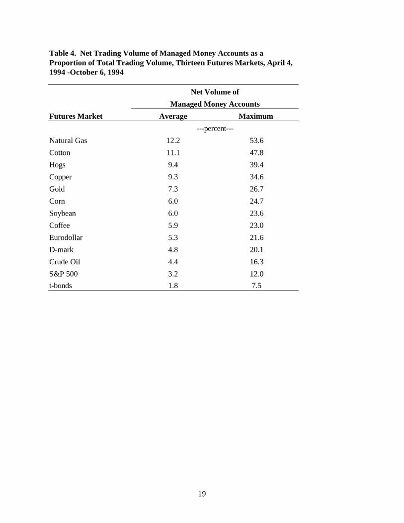
the September corn and soybean contracts are only lightly traded through their existence. Liquidity in these markets shifts in late June from the July contract to the new crop contract (November for soybeans and December for corn). Therefore, in order to follow the liquidity of these markets, a price series was developed which always reflects the most liquid contract. This is referred to as the modified nearby series, and for most markets (except the five listed above) is the equivalent of a nearby price series, which rolls forward at the end of the month previous to expiration. The thirteen markets included in this data set range from the more liquid financial contracts to some of the less liquid agricultural markets. Table 2 reports some general market conditions between April – October 1994, including the average daily trading volume and open interest (for the modified nearby series) and the average daily volatility for futures returns.1 To provide a basis for comparison, Table 2 also reports the ten-year (between 1988 and 1997) average daily volatility measure. These figures suggest volatility for the six-month period being studied is representative of longer-term market conditions. To reach conclusions regarding the effects of MMA trading, it is important to first understand which markets are traded. Any potential effects from their trading may be dependent on whether or not trading is concentrated in the more liquid financial futures or the less liquid markets. The results shown in Table 3 are computed by dividing the net managed money trading volume for each day for each commodity by the total managed money trading volume across all commodities for each day. The results represent the averages of these daily percentages through the six-month data series.2 Consistent with the findings of Irwin and Yoshimaru (1999), the results show that MMA trading volume is significantly concentrated in the most liquid markets. The two most liquid volume markets (T-bond and Eurodollar) account for approximately 45 percent of managed money net trading volume, while only eight percent of managed money net or gross volume is in the four least liquid markets. The concentration of managed money trading volume in the most liquid futures markets suggests that hedge fund operators and CTAs, being well aware of the size of their own trading volume, seek to minimize slippage and other costs associated with large volume orders in less liquid markets. Additionally, this helps minimize any effects their trading may have on destabilizing price movements. Although according to volume figures, MMAs concentrate their trading in more active markets, it is also important to analyze their trading volume relative to the size of each market. The percentages shown in Table 4 equal the average of the daily managed money net (absolute value) trading volume divided by the most liquid contract volume. This shows that although managed money trading is focused in the most liquid markets, their average relative trading volume is largest in the least liquid markets. This is evident by the maximum percentage of the nearby trading volume attributable to managed money accounts. For example, in the natural gas market, MMA trading volume averages 12.22 percent of nearby volume, and the daily maximum percentage of the nearby trading volume is 53.6 percent. Figure 1 provides a graphical representation of this percentage on a daily basis for the natural gas market. These large maximum percentages suggest on certain days MMAs may simultaneously herd into markets. Therefore, although managed money accounts tend to focus their trading in the most liquid

4

markets, thereby decreasing any effects their trading may have on price movements, they may at the same time be increasing these effects through their suspected herding behavior. To gain an understanding of the timing of trading by MMAs relative to trading by the rest of the market, simple correlation coefficients were computed. As reported in Table 5, there is a significant positive correlation (at the five-percent level) between the trading volume of managed money accounts and the rest of the market. The average correlation across all markets is 0.38 on a net basis. These ranged from 0.01 (hog market) to 0.67 (gold market) for the net managed money trading volume. This positive relationship suggests that MMAs are generally trading when everyone else is trading, thereby decreasing any effects they may have on price behavior (relative to other traders). However, it is important to remember that if this were always the case, the large spikes observed in their trading volume as a percent of the market would not exist. Large Hedge Funds, CTAs and Price Volatility Karpoff (1987) provides an extensive summary of the methodology and results of studies focusing on the relationship between volume and volatility. The largest difference between model specifications deals with the accommodations for persistence of volatility and volume. The different methodologies used in studying the relationship between volume and volatility and accommodating persistence in volume and volatility can be summarized by three different studies. Chang, Pinegar, and Schachter (1997) model the volume and volatility relationship without including any specification of past volatility. By including past volatility as an independent variable, Irwin and Yoshimaru (1996) account for the time series properties of volatility. Finally, Bessembinder and Seguin (1993) account for persistence in volume and volatility through the specification of an iterative process.

Due to the lack of a widely accepted model specification for the relationship between volume and volatility and to provide additional validity, each of these three basic specifications is used in the analysis. However, due to the similarity of the results from these different model specifications, only results for a modified version of Chang, Pinegar, and Schachter’s specification is reported.

Chang, Pinegar, and Schachter regress futures price volatility on volume associated with large speculators (as denoted by the CFTC large trader reports) and all other market volume. This basic specification is expanded by including two additional sets of independent variables. Daily effects, on an intra-week basis, on volatility are well documented, implying that a set of daily dummy variables should be included. Therefore, in all regressions estimated, these dummy variables are included. In addition, the estimated specification includes the open interest for each market. As outlined by Bessembinder and Seguin (1993), open interest serves as a proxy for market depth, which is anticipated to have a negative relationship to volatility. This implies that changes in volume have a smaller effect on volatility in a more liquid market (represented by higher open interest). Therefore, the regression model specification for a given futures market is, (1)

1 2 3 4

5 6 7 8 9

t t t t

t t t t t t

MMATV MMAOI AOTV

AOOI Mon Tue Wed Thu

σ β β β ββ β β β β ε

= + + ++ + + + + +

5

where tσ is the daily volatility (standard deviation) of futures returns, MMATVt is the absolute value of managed money net trading volume, MMAOIt is the absolute value of managed money net open interest, AOTVt is other market trading volume, AOOIt is other open interest, Mont, Tuet, Wedt and Thut are dummy variables that represent day-of-the-week effects and ε t is a standard, normal error term. Following Kodres (1994), Irwin and Yoshimaru (1996), and Chang, Pinegar, and Schachter (1997), Parkinson’s (1980) extreme-value estimator is used to estimate daily volatility of futures returns. For a given commodity, Parkinson's estimator is, (2) ˆ ln( / )t t t= 0.601 H Lσ

where Ht is the trading day’s high price and Lt is the day’s low. Wiggins (1991) reports that extreme-value estimators are more efficient than close-to-close estimators.

Previous empirical results suggest that a positive relationship exists between volume and volatility. This relationship should exist with the total market volume as well as with the trading volume of managed money accounts and the rest of the market's trading volume. It is also expected that a negative relationship will be exhibited between volatility and open interest, as shown by Bessembinder and Seguin (1993). However, the fact only six months of data exist might influence this finding. Open interest, within any six-month period may not be variable enough for a regression analysis to estimate this relationship effectively. For the same reason, it is possible that daily dummy variables will not exhibit the U-shape relationship documented in previous studies for volatility.

Table 6 reports the estimated coefficients, corresponding t-statistics, and adjusted R2 for each market. Due to the relative insignificance of the day-of-the week variables, only an F-statistic is reported, which results from testing the joint significance of the dummy variables. As shown by this F-statistic, only the D-mark market is characteristic of significant daily effects. The average adjusted R2 across all thirteen markets is 0.52. The estimated coefficient for managed money trading volume is significantly positive at the five-percent level in nine markets, with the remaining four markets having insignificant coefficients (coffee, cotton, D-mark, and soybeans). All of the estimated coefficients for the rest of market volume are significant and positive at the five-percent level. Therefore, as expected a positive relationship is exhibited between trading volume and price variability, regardless of the trader type (managed money or all other). Four of the estimated coefficients for the managed money open interest are significantly negative (coffee, corn, Eurodollar, and crude oil), while one is significantly positive (natural gas). For the rest of the market’s open interest, coefficients are negative and significant in five markets (coffee, copper, corn, hogs, and crude oil) and significantly positive in one market (S&P 500). As mentioned previously, the relatively mixed results for open interest is not surprising due to the relatively short time period studied. Previous studies (e.g. Chang, Pinegar, and Schachter (1997) estimate the volatility effects of different trader types by comparing the relative sizes of the parameter estimates associated with the traders. For example, the estimates for 2β and 4β from regression model (1) could be compared to determine the volatility effects of MMAs and all other traders. However, this comparison is biased unless the means of the respective independent variables are of similar

6

magnitudes. A better approach is to compare volatility elasticities evaluated at the means of the independent variables.

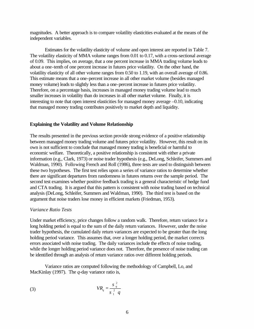
Estimates for the volatility elasticity of volume and open interest are reported in Table 7. The volatility elasticity of MMA volume ranges from 0.01 to 0.17, with a cross-sectional average of 0.09. This implies, on average, that a one percent increase in MMA trading volume leads to about a one-tenth of one percent increase in futures price volatility. On the other hand, the volatility elasticity of all other volume ranges from 0.50 to 1.19, with an overall average of 0.86. This estimate means that a one-percent increase in all other market volume (besides managed money volume) leads to slightly less than a one-percent increase in futures price volatility. Therefore, on a percentage basis, increases in managed money trading volume lead to much smaller increases in volatility than do increases in all other market volume. Finally, it is interesting to note that open interest elasticities for managed money average –0.10, indicating that managed money trading contributes positively to market depth and liquidity. Explaining the Volatility and Volume Relationship The results presented in the previous section provide strong evidence of a positive relationship between managed money trading volume and futures price volatility. However, this result on its own is not sufficient to conclude that managed money trading is beneficial or harmful to economic welfare. Theoretically, a positive relationship is consistent with either a private information (e.g., Clark, 1973) or noise trader hypothesis (e.g., DeLong, Schleifer, Summers and Waldman, 1990). Following French and Roll (1986), three tests are used to distinguish between these two hypotheses. The first test relies upon a series of variance ratios to determine whether there are significant departures from randomness in futures returns over the sample period. The second test examines whether positive feedback trading is a general characteristic of hedge fund and CTA trading. It is argued that this pattern is consistent with noise trading based on technical analysis (DeLong, Schleifer, Summers and Waldman, 1990). The third test is based on the argument that noise traders lose money in efficient markets (Friedman, 1953).

Variance Ratio Tests

Under market efficiency, price changes follow a random walk. Therefore, return variance for a long holding period is equal to the sum of the daily return variances. However, under the noise trader hypothesis, the cumulated daily return variances are expected to be greater than the long holding period variance. This assumes that, over a longer holding period, the market corrects errors associated with noise trading. The daily variances include the effects of noise trading, while the longer holding period variance does not. Therefore, the presence of noise trading can be identified through an analysis of return variance ratios over different holding periods. Variance ratios are computed following the methodology of Campbell, Lo, and MacKinlay (1997). The q-day variance ratio is, (3)

2

21

qqVR

q

σσ

=⋅

7

where 2

qσ is the q-day holding period return variance and 21σ is the daily holding period return

variance. Note that overlapping q-period returns are used to estimate 2qσ and one-day returns are

used to estimate 21σ .3 The use of overlapping returns increases the efficiency of the variance

ratio estimator. For a given commodity, the standardized test statistic to test the null hypothesis that the variance ratio equals one is, (4)

1 / 2

2(2 1)( 1)( 1)

3q q

q qnq VR

qψ

−

=− −

−

where nq+1 is the number of original daily price observations. Campbell, Lo, and MacKinlay show that qψ approximately follows a standard normal distribution in large samples. Variance ratios and associated test statistics are computed for six different holding periods: two, three, five, ten, fifteen, and twenty days.

An important statistical issue arises when interpreting the variance ratio test results. Specifically, what constitutes evidence against the null hypothesis? If variance ratios across holding periods are independent, then rejection of the null hypothesis of unity for one holding period is sufficient to reject the joint null hypothesis that variance ratios equal unity across all holding periods. It is unlikely that the independence assumption is valid due to the overlapping nature of the holding periods. As a result individual hypothesis tests likely have a higher probability of Type I error than the specified significance level.

To correctly assess the joint significance of variance ratios across holding periods a joint

test statistic is needed. The Bonferroni inequality provides a simple means for testing the joint null hypothesis that test statistics are not different from one. The inequality provides an upper bound for rejection of the joint null hypothesis when the test statistics are correlated. Intuitively, the Bonferroni test simple scales up the p-value of the most significant test statistic to account for the dependency. Miller (1966) provides a full explanation of the Bonferroni inequality and resulting joint testing procedure.

To implement the Bonferroni joint test for a given commodity, define the maximum standardized test statistic as, (5) { }max max q =

q ψψ

where qψ is the standardized test statistic for the q-day holding period. Next, the joint null

hypothesis is rejected at the significance level α if maxψ is greater than the critical value defined by,

8

(6) ( )*

2/c

1 - = αψΦ

where ( )Φ i represents the standard normal cumulative distribution function and c is the number of restrictions tested. Since variance ratios are estimated for six holding periods, a joint hypothesis test for a given futures market imposes six restrictions. As a result, the critical value for the Bonferroni joint test is 2.63.

Variance ratios and standardized test statistics for each of the thirteen markets are presented in Table 8. There are only two variance ratios out of 78 where the null hypothesis of unity is rejected. The two significant ratios suggest the possibility of short-run noise trading component in the gold market. The significant negative test statistics for the two-day and three-day holding periods indicate that two- and three-day holding period return variances are less than two and three times the estimated daily variance. This implies the daily return variances are larger due to the noise component. However, this noise component is traded away in the long run, as shown by the insignificant test statistics for the longer holding periods. providing strong support for the private information hypothesis.

The gold market also is the only market out of thirteen where the Bonferroni joint test

statistic is significant. This rejection rate (0.077) is only slightly greater than would be expected based on random chance and a five-percent significance level. Overall, the variance ratio tests for this sample period do not support the noise trader hypothesis, but instead support the private information hypothesis for managed money account trading.

Since the sample period considered in the above tests is somewhat limited (April 4, 1994-

October 6, 1994), a reasonable question is whether the results are sensitive to different time periods and longer sample periods. The first alternative sample period considered is the previous six-month period from October 1993 through March 1994.4 In this case, only six of 78 variance ratios are significantly different from one. The Bonferroni joint test statistic is significant only for the eurodollar futures market, which, again, is only slightly greater than would be expected based on random chance. The second alternative sample period considered is substantially longer and includes the previous six and one-quarter year period from January 1988 through March 1994. In this case, only seventeen out of 78 variance ratios are significantly different from one. However, the Bonferroni joint test statistic is significant for four of the thirteen markets (cotton, eurodollar, crude oil and the S&P 500), more than would be expected based on random chance.

The last finding indicates that variance ratio test results may be somewhat sensitive to the

use of a relatively small sample size. Nonetheless, the variance ratio results for alternative sample periods do not provide convincing evidence that the conclusion reached on the basis of the original sample period is invalid. That is, variance ratio tests do not indicate substantial deviations from market efficiency that would be associated with noise trading on the part of managed money accounts. Instead, the results are most consistent with the hypothesis that managed money accounts base their trading on valuable private information.

9

Positive Feedback Trading Tests Positive feedback trading is characterized by buying after price increases and selling after declines in price. The existence of this type of trading may lead to decreases in market efficiency by creating excessive volatility. For instance, when new bullish fundamental information is received, and price increases to its new fundamental value through rational trading, positive feedback traders continue to buy, driving price past its rational value. Following Kodres and Irwin and Yoshimaru, positive feedback trading may be identified for a given market by estimating the following regression model, (7)

5

11

t i t i ti

NETMMATV pα β ε−=

= + ∆ +∑

where NETMMATVt is the net trading volume of managed money accounts (number of long contracts minus number of short contracts) on day t, t ip −∆ is the continuously-compounded futures return on day t-i and ε t is a standard, normal error term. For simplicity, five lagged price returns are included in the model for all markets. Note that NETMMATVt takes on positive values when MMAs are net buyers of contracts, negative values when MMAs are net sellers, and zero when no volume is recorded. Slope coefficients in (7) can be thought of as the sensitivities of MMA "demand" to past price movements. Positive slope coefficients are evidence of positive feedback trading by MMAs, whereas negative coefficients are evidence of negative feedback trading. The net feedback effect is given by the sum of slope coefficients for each regression. The significance of feedback trading is identified by testing whether the sum of the estimated slope coefficients (for lagged price returns) is greater than zero.

The results for the estimation of this equation are given in Table 9. The average adjusted R2 across all thirteen markets is 0.088, ranging from a high of 0.347 (cotton) to a low of -0.017 (coffee). The t-statistic testing the sum of the coefficients is positive and significant in eight of the thirteen markets. This seems to provide evidence supporting the hypothesis that managed money trading can be characterized as noise trading. However, a distinction between statistical and economic significance may suggest otherwise. Although, statistical significance can not be disputed in eight markets, with an average adjusted R2 across all thirteen markets of 0.088, it can be concluded that positive feedback trading (across all markets) is responsible for, on average, only 8.8 percent of the variance in managed money trading. It is, therefore, more reasonable to conclude that trading decisions by MMAs, although influenced in small part by past price changes (statistical significance), are not driven (economic significance) by past price changes.

An additional frame of comparison is made by analyzing the positive feedback characteristics of the Commitment of Trader data as reported by the CFTC. The weekly reported open interest figures for each week of 1994 were used to compute commercial and non-commercial reporting traders’ estimated minimum trading volume (using the same methodology as previously outlined for the MMA data set). Regression model (7) is then estimated using these weekly volume estimates and weekly price changes. The results for the reporting commercial and non-commercial traders are given in Tables 10 and 11, respectively. On a weekly basis, past price changes generally explain much more of the trading volume by these trading categories, than for the MMA trading volume. The non-commercial category is

10

characteristic of positive feedback trading, with a significant t-statistic (testing whether the sum of the coefficients is greater than zero) in twelve of the thirteen markets. The commercial category, on the other hand, is characteristic of negative feedback trading (testing whether the sum of the coefficients is less than zero), with significant t-statistics in eleven of the thirteen markets. This implies the positive feedback characteristics of non-commercial traders may actually result from taking the opposite side of commercial trades.

The previous interpretation is better understood after considering a common trading characteristic of commercial traders. It is common for commercial processors to employ scale down buying techniques: increasing their buying as prices decrease. It is also commonplace for commercial producers to sell on a scale up strategy, or selling increasing amounts of their production as prices increase. This type of trading action is characteristic of negative feedback trading. If employed in this fashion, those taking the opposite side of these commercial orders become identified as positive feedback traders. It is therefore, not a surprise that non-commercial traders are characteristic of positive feedback trading. This explanation implies that non-commercial traders are acting to provide the market liquidity needed by commercial firms. Although their trading actions may be motivated by technical analysis or trend following indicators, it is apparent their trading behavior corresponds to the liquidity needs of commercial interests.

Profitability Tests

According to Friedman (1953), in order for speculation to be destabilizing, speculators must be buying when prices are above fundamental value and selling when prices are below. This process creates excessive volatility by driving price past its fundamental value. Rational speculators, however, recognizing the deviation from fundamentals take the opposite position bringing prices back to reflect the underlying fundamentals. Rational speculators, therefore, make a profit while destabilizing speculators lose money. The following analysis of managed futures estimated profits is based on this theoretical foundation. The estimates of profits by MMAs during this six-month period are based on the mark-to-market technique used by Hartzmark (1987) and Leuthold, Garcia and Lu (1994). The price change (based on the close-to-close difference) on day t is multiplied by the net open interest position held by managed money accounts at the end of day t-1. The daily profit/loss figures are then aggregated across all days for each market to compute a total profit or loss for each market over the entire six-month period. Although this analysis is based on a short time period, aggregating across all markets provides additional validity. Under the assumption of market price independence across the thirteen markets (which is obviously not true for some of the markets, like corn and soybeans), this analysis can be likened to using 78 months of data for one market (six months multiplied by thirteen markets). The profit/loss estimates are presented in Table 12 for each market and aggregated across all markets. The estimated profits and losses for the entire six-month period range from a high of $430.7 million (coffee) to low of -$234.5 million (S&P 500). The aggregated total across all thirteen markets is a profit of $397.6 million. The estimated profit across all thirteen markets provides evidence, which suggests, once again, that trading by managed money accounts is not best characterized as noise trading during this six-month period. Under the assumption of an

11

efficient market, in order for speculative activity to be destabilizing, speculators must be buying when prices are high and selling when prices are low. Trading in this manner must lead to trading losses, when the market price returns to its underlying fundamental value. The profit estimates reported here, however, suggest that managed money accounts are not destabilizing, but instead are based upon valuable private information. Summary and Conclusions The trading behavior of hedge funds and commodity trading advisors (CTAs) has been the subject of considerable attention in recent years. Despite the considerable interest in the market behavior and impact of hedge funds and CTAs, a limited number of academic studies investigate the issue. The limited nature of previous research on the market impact of hedge funds and CTAs can be traced directly to the difficulty of obtaining data on their trading activities. The CFTC’s large trader reporting system does not routinely flag positions held by hedge funds and CTAs, so there is no regular reporting on their trading. However, the CFTC did conduct a special project to gather comprehensive data on the trading activities of large hedge funds and CTAs in thirteen futures markets between April 1994 and October 1994.

This study uses the newly available data from the CFTC to investigate the market impact

of futures trading by large hedge funds and CTAs. The first part of the paper analyzes the relationship between hedge fund and CTA trading and market volatility. Drawing upon the specifications of Bessembinder and Seguin (1993) and Chang, Pinegar and Schacter (1997), regression models of market volatility are expressed as a function of: i) trading volume and open interest for large hedge funds and CTAs, ii) trading volume and open interest for the rest of the market and iii) day-of-the week effects. The regression results show that there is a positive relationship between the trading volume of large hedge funds and CTAs and market volatility. However, a positive relationship between hedge fund and CTA trading volume and market volatility is consistent with either a private information (e.g., Clark, 1973) or noise trader hypothesis (e.g., DeLong, Schleifer, Summers and Waldman, 1990).

The second part of the paper conducted tests to distinguish between the private information hypothesis and the noise trader hypothesis. The first test consisted of identifying the noise component exhibited in return variances over different holding periods. The efficient market hypothesis implies that a q day holding period return variance should be equal to q times the daily return variance. Only two of 78 estimated test statistics are significant, suggesting that a statistically identifiable noise component only exists in one market (gold). Even in this market, however, the noise component is not significant for holding period returns greater than three days. Therefore, it may be concluded from the results of these variance ratio tests, that there is little support for the noise trader hypothesis during this six-month period.

The second test examined whether positive feedback trading characterized large hedge

fund and CTA trading behavior. The average adjusted R2 for positive feedback regressions across all thirteen markets is only 0.088, ranging from a high of 0.347 (cotton) to a low of -0.017 (coffee). While there is evidence of statistically significant positive feedback trading in eight markets, with an average adjusted R2 across all thirteen markets of 0.088, it can be concluded

12

that positive feedback trading (across all markets) is responsible for, on average, only 8.8 percent of the variance in managed money trading. It is, therefore, more reasonable to conclude that trading decisions by large hedge funds and CTAs, although influenced in small part by past price changes (statistical significance), are not driven (economic significance) by past price changes.

The third test consists of estimating the profits and losses associated with the open

interest positions of large hedge funds and CTAs. According to Friedman (1953), in order for speculative trading to be destabilizing, speculators must be buying when prices are above fundamentals and selling when price is below. The implication of this hypothesis is that destabilizing speculators lose money and are driven from the market, having no negative long term effects on market efficiency. The profits and losses were estimated for each day and then aggregated for each market. Across all thirteen markets, the profit for large hedge funds and CTAs are estimated to be just under $400 million. This implies that the trading decisions of are likely based on valuable private information.

Overall, the evidence presented in this study suggests trading by large hedge funds and CTAs is based on private fundamental information. Futures return variances exhibited a significant noise component in only one market. In addition, large hedge funds and CTAs generated nearly $400 million in gross trading profits across all thirteen markets. These findings imply large hedge funds and CTAs benefit market efficiency by bringing valuable, fundamental information to the market through their trading.

13

References

Bessembinder, H. and Seguin, P. “Price Volatility, Trading Volume, and Market Depth: Evidence from Future Markets.” Journal of Financial and Quantitative Analysis. 28(1993):21-39.

Brorsen, B.W. and S.H. Irwin. "Futures Funds and Price Volatility." Review of Futures

Markets. 61(1987):119-135 Brown, S.J., W.N. Goetzmann, and J. Park. “Hedge Funds and the Asian Currency Crisis of

1997.” Working Paper 6427, National Bureau of Economic Research, February 1998. Campbell, J.Y., A.W. Lo and A.C. MacKinlay. The Econometrics of Financial Markets.

Princeton, NJ: Princeton University Press, 1997. Chang, E.C., M.J. Pinegar, and B. Schachter. “Interday Variations in Volume, Variance, and

Participation of Large Speculators .” Journal of Banking and Finance. 21(1997):797-910.

Clark, P.K. "A Subordinated Stochastic Process Model with Finite Variance for Speculative

Prices." Econometrica. 41(1973):135-155. De Long, J.B., A. Schleifer, L.H. Summers, and R.J. Waldman. "Noise Trader Risk in Financial

Markets." Journal of Political Economy. 98(1990)., 703-738. French, K. and R. Roll. “Stock Return Variances.” Journal of Financial Economics.

17(1986):5-26. Friedman, M. “The Case for Flexible Exchange Rates.” in Essays in Positive Economics.

University of Chicago Press: Chicago, 1953, pp. 157-203. Fung, W. and Hsieh, D. “Empirical Characteristics of Dynamic Trading Strategies: The Case of

Hedge Funds.” The Review of Financial Studies. 10(1997):275-302. Hartzmark, M.L. “Returns to Individual Traders of Futures: Aggregate Results.” Journal of

Political Economy. 95(1987):1292-1306. Irwin, S.H. and Yoshimaru, S. “Managed Futures, Positive Feedback Trading, and Futures Price

Volatility.” Journal of Futures Markets. 19(1999):759-776. Karpoff, J. “The Relation Between Price Changes and Trading Volume: A Survey.” Journal of

Financial and Quantitative Analysis. 22(1987):109-126. Kodres, Laura. “The Existence and Impact of Destabilizing Positive Feedback Traders:

Evidence from the S&P 500 Index Futures Market.” Working Paper, Board of Governors of the Federal Reserve System, 1994.

14

Leuthold, R. P. Garcia, and R. Lu. “The Returns and Forecasting Ability of Large Traders in the

Frozen Pork Bellies Futures Market.” Journal of Business. 64(1994):459-477. Mielke, J. “Personal Communication.” Division of Economic Analysis, Commodity Futures

Trading Commission, October 1998. Miller, R.G. Simultaneous Statistical Inference. McGraw-Hill Book Company: New York,

1966. Parkinson, M. "The Extreme Value Method for Estimating the Variance of the Rate of Return."

Journal of Business 64(1980):417-432. Ross, M. "CBOT, IFB Trade Observations." Farm Week, September 20, 1999, pp.1,3. Wiggins, J.G. "Empirical Tests of the Bias and Efficiency of the Extreme-Value Variance

Estimator for Common Stock." Journal of Business 64(1991):417-432.

15

Endnotes 1 Daily volatility is estimated by Parkinson’s (1980) extreme-value (high-low) volatility estimator. Further details are provided in the next section. 2 All analysis in this study also is computed on a gross basis. The results are similar, so that only the net volume results are reported. 3 The formula’s for the variance estimators are found on pp. 52-53 in Campbell, Lo and MacKinlay (1997). One technical issue is how to handle the computation of futures returns when nearby futures price series roll from the “old” nearby contract to the “new” nearby contract. To resolve this issue, returns for the first active day of the “new” nearby contract are computed using the previous day’s price for the “new” contract, rather than the previous day’s price from the “old” contract. 4 The variance ratio test results for alternative sample periods are available from the authors upon request.

Exchange Designated Referenced Futures Trading

Futures Contract Name Market Name Exchange Symbol Units

Coffee "C" Coffee CSCE KC ¢/lb

High-grade copper Copper COMEX HG ¢/lb

Corn Corn CBOT C ¢/bu

Cotton Cotton NYCE CT ¢/lb

Deutsche Mark D-mark CME DM ¢/D-mark

Eurodollar time deposit Eurodollar CME ED Pts of 100%

Gold Gold COMEX GC $/OZ

Live hogs Hog CME LH ¢/lb

Henry hub natural gas Natural Gas NYMEX NG $/MMBtu

Light, sweet crude oil Crude Oil NYMEX CL $/BBL

Soybeans Soybean CBOT S ¢/bu

Standard & Poor's 500 S&P 500 CME SP Index

US 30-year treasury bonds t-bond CBOT US Pts of 100%

Table 1. Futures Market Names, Exchanges, Trading Symbols, and Units

16

Futures Jan. 1988-Dec. 1997

Market Volume Open Interest Volatility Volatility

---percent--- ---percent---

Coffee 8,036 24,469 2.60 1.69

Copper 7,919 32,860 1.03 1.15

Corn 23,072 123,906 0.90 0.84

Cotton 5,091 26,660 0.92 0.88

D-mark 42,530 93,056 0.47 0.46

Eurodollar 119,143 456,811 0.05 0.05

Gold 28,230 83,151 0.49 0.52

Hog 2,576 12,296 1.01 0.95

Natural Gas 9,214 22,766 1.69 1.77

Crude Oil 49,609 97,726 1.43 1.33

Soybean 26,922 68,876 0.89 0.88

S&P 500 65,700 190,626 0.52 0.68

t-bond 392,204 363,407 0.61 0.49

Apr. 4, 1994 - Oct. 6, 1994

Daily Average

---contracts---

Table 2. Average Levels of Volume, Open Interest and Volatility, Thirteen Futures Markets, April 4, 1994 -October 6, 1994.

17

Futures Market Proportion of Total Trading Volume

--percent---

Coffee 1.7

Copper 3.0

Corn 5.7

Cotton 2.6

Crude Oil 8.4

D-mark 7.3

Eurodollar 22.9

Gold 8.0

Hog 0.9

Natural Gas 4.5

S&P 500 7.1

Soybean 6.1

t-bond 21.8

100.0

Table 3. Distribution of Managed Money Account Trading Volume Across Thirteen Futures Markets, April 4, 1994 -October 6, 1994

18

Futures Market Average Maximum

Natural Gas 12.2 53.6

Cotton 11.1 47.8

Hogs 9.4 39.4

Copper 9.3 34.6

Gold 7.3 26.7

Corn 6.0 24.7

Soybean 6.0 23.6

Coffee 5.9 23.0

Eurodollar 5.3 21.6

D-mark 4.8 20.1

Crude Oil 4.4 16.3

S&P 500 3.2 12.0t-bonds 1.8 7.5

Net Volume of

---percent---

Managed Money Accounts

Table 4. Net Trading Volume of Managed Money Accounts as a Proportion of Total Trading Volume, Thirteen Futures Markets, April 4, 1994 -October 6, 1994

19

Futures Market Correlation Coefficient

Coffee 0.33*

Copper 0.50*

Corn 0.58*

Cotton 0.64*

D-mark 0.44*

Eurodollar 0.35*

Gold 0.67*

Hogs 0.01

Natural Gas 0.06

Crude Oil 0.21*

Soybean 0.56*

S&P 500 0.25*

t-bond 0.31*

Note: A star indicates statistical significance at the five percent level of significance.

Table 5. Correlation between Managed Money Account Trading and All Other Market Trading Volume, Thirteen Futures Markets, April 4, 1994 -October 6, 1994

20

Rest of MMA Net Rest ofFutures MMA Net Nearby Open Nearby Open Adj.Market Intercept Volume Volume Interest Interest R 2 F -Statistic

Coffee 3440.1* -0.12 0.4590* -0.1444* -0.1831* 0.51 1.31(6.39) (-0.73) (11.19) (-4.85) (-6.31)

Copper 522.6* 0.0973* 0.1091* -0.0018 -0.0214* 0.61 1.12(3.98) (3.22) (9.67) (-0.37) (-4.53)

Corn 916.5* 0.0411* 0.0253* -0.0147* -0.0046* 0.49 1.15(3.17) (2.30) (6.41) (-3.53) (-1.98)

Cotton 331.7 0.0379 0.1279* 0.0070 -0.0009 0.41 0.97(1.57) (0.98) (6.77) (0.71) (-0.14)

D-mark 184.5 0.0088 0.0121* 0.0019 -0.0019 0.45 4.06*(1.64) (1.09) (7.94) (1.01) (-1.57)

Eurodollar 35.7 0.0010* 0.0004* -0.0002* -0.00001 0.69 0.38(1.60) (3.69) (11.61) (-3.88) (-0.24)

Gold 74.7 0.0234* 0.0154* -0.0010 -0.0003 0.63 2.07(0.71) (3.60) (7.97) (-0.77) (-0.29)

Hogs 290.0 0.3929* 0.2272* 0.0081 -0.0306* 0.30 1.10(1.04) (3.55) (5.74) (0.29) (-3.05)

Natural Gas 120.6 0.1115* 0.1399* 0.0256* 0.0036 0.47 0.52(0.42) (2.76) (8.94) (2.51) (0.26)

Crude Oil 739.4* 0.0539* 0.0357* -0.0189* -0.0094* 0.44 1.85(2.69) (2.24) (9.05) (-4.22) (-3.38)

Soybeans -121.2 0.0140 0.0423* -0.0132 -0.0003 0.57 1.05(-0.44) (0.71) (9.94) (-1.61) (-0.09)

S&P 500 -657.7 0.0268* 0.0099* -0.0008 0.0035* 0.53 1.03(-3.61) (3.34) (10.19) (-0.45) (3.79)

t-bonds 83.8 0.0126* 0.0018* -0.0006 -0.0006 0.69 2.16(0.78) (4.75) (12.96) (-0.39) (-1.93)

Table 6. Estimation Results for Volatility Regression Models, Thirteen Futures Markets, April 4, 1994 -October 6, 1994.

Note: The figures in parentheses are t -statistics. The F -statistic tests the null hypothesis that parameters on the day-of-the week dummy variables jointly equal zero. A star indicates statistical significance at the five percent level of significance.

21

Futures MMA Net Rest of Nearby MMA Net Rest of Nearby

Market Volume Volume Open Interest Open Interest

Coffee 0.01 1.19 -0.38 -0.94

Copper 0.09 0.76 -0.04 -0.39

Corn 0.09 0.50 -0.15 -0.49

Cotton 0.02 0.59 0.04 -0.04

Crude Oil 0.16 0.88 -0.14 -0.38

D-Mark 0.05 1.04 0.05 -0.30

Eurodollar 0.13 1.05 -0.80 -0.19

Gold 0.17 0.71 0.00 -0.08

Hogs 0.11 0.51 0.14 -0.06

Natural Gas 0.07 0.64 0.11 -0.05

S&P 500 0.12 1.18 0.00 0.98

Soybeans 0.03 1.09 -0.10 0.01

t-bonds 0.15 1.09 0.01 -0.35

Table 7. Estimates of the Volatility Elasticity of Volume and Open Interest, Thirteen Futures Markets, April 4, 1994 - October 6, 1994.

22

Futures BonferrroniMarket 2 Day 3 Day 5 Day 10 Day 15 Day 20 Day Joint Test Statistic

Coffee 1.08 1.12 1.19 1.25 1.49 1.53 1.21(0.86) (0.95) (1.00) (0.84) (1.32) (1.21)

Copper 0.92 0.91 0.92 0.96 0.97 1.00 0.86(-0.86) (-0.69) (-0.42) (-0.15) (-0.07) (0.00)

Corn 0.97 1.07 0.96 0.78 0.98 1.00 0.72(-0.3) (0.56) (-0.19) (-0.72) (-0.06) (0.01)

Cotton 1.08 1.06 1.10 0.99 0.98 0.86 0.91(0.91) (0.45) (0.52) (-0.03) (-0.06) (-0.32)

D-mark 1.02 1.04 1.09 1.01 0.78 0.73 0.61(0.17) (0.30) (0.49) (0.04) (-0.60) (-0.61)

Eurodollar 1.12 1.19 1.16 0.78 0.74 0.71 1.43(1.39) (1.43) (0.81) (-0.75) (-0.69) (-0.67)

Gold 0.71* 0.72* 0.70 0.75 0.65 0.61 3.25*(-3.25) (-2.16) (-1.58) (-0.86) (-0.94) (-0.90)

Hog 1.03 0.97 0.90 0.84 0.74 0.51 1.11(0.35) (-0.21) (-0.54) (-0.54) (-0.69) (-1.11)

Natural Gas 0.97 1.06 1.24 1.24 1.18 1.19 1.24(-0.29) (0.44) (1.24) (0.81) (0.49) (0.43)

Crude Oil 1.09 1.09 1.02 1.26 1.35 1.58 1.33(1.00) (0.68) (0.11) (0.89) (0.93) (1.33)

Soybean 1.03 1.09 0.96 0.82 0.99 0.98 0.69(0.31) (0.69) (-0.23) (-0.59) (-0.02) (-0.03)

S&P 500 0.84 0.93 0.86 0.74 0.75 0.73 1.86(-1.86) (-0.52) (-0.71) (-0.87) (-0.66) (-0.61)

t-bond 0.88 0.86 0.77 0.52 0.49 0.48 1.63(-1.35) (-1.06) (-1.18) (-1.63) (-1.37) (-1.19)

Holding Period Lengths

Table 8. Variance Ratio Test Results, Thirteen Futures Markets, April 4, 1994 -October 6, 1994

Note: The figures in parentheses are Z -statistics. A star indicates statistical significance at the five percent level of significance.

23

Futures Price Change Lag Adj.Market t-1 t-2 t-3 t-4 t-5 R 2 t -statistic

Coffee -2.8 12.8 1.4 7.3 2.6 -0.02 0.98(-0.31) (1.44) (0.15) (0.82) (0.28)

Copper 20.1 214.2* 38.9 141.1 -24.2 0.05 2.23*(0.27) (2.84) (0.52) (1.87) (-0.31)

Corn 251.7* 190.5* -8.4 -61.6 170.0* 0.15 3.77*(3.85) (3.12) (-0.14) (-1.01) (2.62)

Cotton 628.7* 214.8* 230.7* 63.8 196.4* 0.35 6.83*(7.03) (2.39) (2.57) (0.71) (2.23)

D-mark -160.9 1729.7* 468.3 553.2 77.4 0.01 1.76*(-0.22) (2.38) (0.64) (0.76) (0.11)

Eurodollar -21276.9 8063.6 -6149.2 -25505.1 -15490.5 0.02 -2.10*(-1.52) (0.58) (-0.44) (-1.83) (-1.11)

Gold 27.6 543.2* 405.8* 41.5 76.1 0.07 2.74*(0.17) (3.24) (2.41) (0.25) (0.47)

Hogs 183.2* 139.2* 64.0 83.7 71.3 0.11 4.01*(3.26) (2.48) (1.14) (1.5) (1.27)

Natural Gas -619.6 16136.4* 11659.5* -3158.6 -533.1 0.14 2.97*(-0.16) (4.05) (2.92) (-0.79) (-0.13)

Crude Oil -381.8 712.4 -445.0 2117.2* -29.8 0.02 0.9095(-0.44) (0.82) (-0.52) (2.44) (-0.03)

Soybean 42.2 55.2* -1.6 -0.2 6.1 0.05 1.89*(1.92) (2.66) (-0.08) (-0.01) (0.28)

S&P 500 -135.8 190.6* -62.7 -192.2* 8.4 0.04 -0.978(-1.48) (2.08) (-0.65) (-2.03) (0.09)

t-bond -4888.7* 669.0 68.4 -1422.8 -132.5 0.14 -1.547(-4.67) (0.64) (0.07) (-1.37) (-0.13)

Table 9. Estimation Results for Positive Feedback Regression Models, Managed Money Accounts, Thirteen Futures Markets, April 4, 1994 -October 6, 1994.

Note: The figures in parentheses are t -statistics to test the null hypothesis that a given slope parameter equals zero. The figures in the last column under t -statistic test the null hypothesis the sum of the slope parameters for a given market equals zero. A star indicates statistical significance at the five percent level of significance.

24

Futures Price Change Lag Adj.Market t-1 t-2 t-3 t-4 t-5 R 2 t -statistic

Coffee 30.38 4.81 -27.87 -1.93 1.55 -0.05 0.16(1.26) (0.21) (-1.16) (-0.08) (0.06)

Copper 358.64* 218.37* 102.13 -230.84* -173.06 0.34 1.12(3.38) (2.06) (0.98) (-2.23) (-1.67)

Corn 3957.61* 7.52 113.73 1876.59 -701.27 0.18 2.38*(3.46) (0.01) (0.10) (1.64) (-0.61)

Cotton 736.20* 686.87* 101.61 -20.19 -232.41 0.40 3.64*(4.49) (4.01) (0.62) (-0.12) (-1.37)

D-mark 8500.73* 959.10 -900.51 -1756.04 -844.27 0.49 1.71*(6.61) (0.75) (-0.70) (-1.37) (-0.66)

Eurodollar 15759.56 -17710.66 1094.93 17072.40 -5494.86 -0.01 0.23(0.95) (-1.09) (0.06) (1.03) (-0.32)

Gold 2395.01* 861.22* 317.18 108.46 92.06 0.74 6.65*(11.05) (3.97) (1.52) (0.52) (0.45)

Hog 65.47 297.49 136.43 52.05 101.34 0.00 1.90*(0.4) (1.87) (0.87) (0.33) (0.64)

Natural Gas 20531.08* 7204.19 2533.47 99.04 2197.54 0.12 2.15*(3.33) (1.23) (0.44) (0.02) (0.41)

Crude Oil 11002.22* -1612.33 -295.64 -759.42 1121.72 0.60 2.86*(7.94) (-1.15) (-0.21) (-0.55) (0.77)

Soybean 1224.71* 593.45* 31.72 273.57 192.01 0.45 4.38*(5.68) (2.88) (0.16) (1.33) (0.89)

S&P 500 325.63* 61.07 105.54 -111.13 -217.41* 0.19 0.55(3.07) (0.56) (0.95) (-1.00) (-2.06)

t-bond 3292.31* -940.62 -197.80 -403.86 1620.73 0.04 -0.03(2.15) (-0.59) (-0.12) (-0.25) (1.06)

Table 10. Estimation Results for Positive Feedback Regression Models, Non-Commercial Firms, Thirteen Futures Markets, January - December 1994

Note: The figures in parentheses are t -statistics to test the null hypothesis that a given slope parameter equals zero. The figures in the last column under t -statistic test the null hypothesis the sum of the slope parameters for a given market equals zero. A star indicates statistical significance at the five percent level of significance.

25

Futures Price Change Lag Adj.Market t-1 t-2 t-3 t-4 t-5 R 2 t -statistic

Coffee -23.24 -20.45 29.80 3.98 7.48 -0.04 -0.07(-0.9) (-0.83) (1.16) (0.16) (0.29)

Copper -397.78* -163.58 -151.32 340.89* 187.81 0.27 -0.56(-2.8) (-1.15) (-1.09) (2.46) (1.35)

Corn -5531.57* -330.07 109.26 -2022.77 506.59 0.26 -2.92*(-4.29) (-0.26) (0.08) (-1.57) (0.39)

Cotton -872.87* -813.73* -77.93 -23.88 277.11 0.40 -3.58*(-4.41) (-3.93) (-0.39) (-0.12) (1.35)

D-mark -12334.13* -1510.32 415.17 1821.70 1260.60 0.54 -2.25*(-7.26) (-0.89) (0.24) (1.08) (0.74)

Eurodollar -21846.75 23183.32 18208.15 2174.18 25372.70 -0.03 0.65(-0.84) (0.91) (0.68) (0.08) (0.95)

Gold -3287.33* -971.21* -470.79 -189.77 83.31 0.76 -6.64*(-11.81) (-3.49) (-1.76) (-0.71) (0.32)

Hog 173.23 -125.52 -123.42 13.24 -155.35 0.04 -0.95(1.6) (-1.18) (-1.18) (0.13) (-1.47)

Natural Gas -22158.76* -8098.40 1068.06 1002.62 -2214.41 0.12 -1.82*(-3.25) (-1.25) (0.17) (0.16) (-0.38)

Crude Oil -17143.6* -939.56 1738.99 2338.45 935.28 0.55 -2.32*(-7.27) (-0.39) (0.73) (1.00) (0.38)

Soybean -1360.09* -625.50* 81.74 -553.50* -169.78 0.53 -5.22*(-6.62) (-3.19) (0.43) (-2.82) (-0.83)

S&P 500 -115.51 -125.88 -234.96 29.60 110.28 0.00 -0.94(-0.9) (-0.95) (-1.75) (0.22) (0.86)

t-bond -2370.26 726.26 1025.15 -376.98 -1338.79 -0.05 -0.47(-1.31) (0.38) (0.54) (-0.2) (-0.74)

Table 11. Estimation Results for Positive Feedback Regression Models, Non-Commercial Firms, Thirteen Futures Markets, January - December 1994

Note: The figures in parentheses are t -statistics to test the null hypothesis that a given slope parameter equals zero. The figures in the last column under t -statistic test the null hypothesis the sum of the slope parameters for a given market equals zero. A star indicates statistical significance at the five percent level of significance.

26

EstimatedFutures Market Profit/Loss

Coffee $430,716,375

Copper $73,005,900

Corn -$14,938,488

Cotton -$51,881,390

D-mark $50,182,112

Eurodollar $267,424,525

Gold -$81,713,100

Hog $41,935,010

Natural Gas $63,151,300

Crude Oil $91,460,660

Soybean -$44,282,338

S&P 500 -$234,502,500

t-bond -$192,971,969

Total $397,586,099

Table 12. Estimated Profits for Managed Money Accounts, Thirteen Futures Markets, April 4, 1994-October 6, 1994

27

Figure 1. Managed Money Trading Volume as a Proportion of Total Nearby Trading Volume, Natural Gas Futures Market, April 4, 1994 - October 6, 1994

0

0.1

0.2

0.3

0.4

0.5

0.604

-Apr

-94

14-A

pr-9

4

26-A

pr-9

4

09-M

ay-9

4

19-M

ay-9

4

01-J

un-9

4

13-J

un-9

4

23-J

un-9

4

06-J

ul-9

4

18-J

ul-9

4

28-J

ul-9

4

09-A

ug-9

4

19-A

ug-9

4

31-A

ug-9

4

13-S

ep-9

4

23-S

ep-9

4

05-O

ct-9

4

Pro

port

ion

of T

radi

ng V

olum

e

28