The Effect of Increasing Human Capital Investment on

Economic Growth and Poverty: A Simulation Exercise

Bravo Working Paper # 2020-003

Matthew Collin∗ Brookings Institution David N. Weil† Brown University

Abstract: We examine the dynamic responses of income and poverty to increased investment in the human capital of new cohorts of workers, using a quantitative macroeconomic model with realistic demography. Compared to a baseline in which the rate of human capital investment currently observed in every country remains constant we examine two alternative scenarios: one in which each country experiences a rate of growth of human capital investment that is typical of what was observed in the decade ending in 2015, and one in which each country raises human capital investment at a rate corresponding to the 75th percentile of what was observed in the data. In the former, world GDP per capita is 5% higher than baseline in the year 2050, while the global rate of $1.90 poverty is 0.7 percentage points lower in that year. In the latter, world GDP per capita is 12% higher than baseline in 2050, while the rate of $1.90 poverty drops by 1.4 percentage points. These gains are concentrated in poor countries. We argue in the context of our model that investing in people is more cost effective than investing in physical capital as a means to achieve specified income or poverty goals.

Keywords: Human Capital, Economic Growth JEL classification: I10,I20,O4

____________________________________________ ∗Email: mcollin@brookings.edu, Thank you to Aart Kraay, Roberta Gatti, Ritika Dsouza, Nicola Dehnen, Maria Ana Lugo, and Daniel Mahler for helpful comments, suggestions and access to data. †Email: david weil@brown.edu

The Effect of Increasing Human Capital Investment on

Economic Growth and Poverty: A Simulation Exercise

Matthew Collin∗

Brookings Institution

David N. Weil†

Brown University

October 2019

Abstract

We examine the dynamic responses of income and poverty to increased investment

in the human capital of new cohorts of workers, using a quantitative macroeconomic

model with realistic demography. Compared to a baseline in which the rate of human

capital investment currently observed in every country remains constant we examine

two alternative scenarios: one in which each country experiences a rate of growth of

human capital investment that is typical of what was observed in the decade ending

in 2015, and one in which each country raises human capital investment at a rate

corresponding to the 75th percentile of what was observed in the data. In the former,

world GDP per capita is 5% higher than baseline in the year 2050, while the global

rate of $1.90 poverty is 0.7 percentage points lower in that year. In the latter, world

GDP per capita is 12% higher than baseline in 2050, while the rate of $1.90 poverty

drops by 1.4 percentage points. These gains are concentrated in poor countries. We

argue in the context of our model that investing in people is more cost effective than

investing in physical capital as a means to achieve specified income or poverty goals.

Keywords: Human Capital, Economic Growth

JEL classification: I10,I20,O4

∗Email: mcollin@brookings.edu, Thank you to Aart Kraay, Roberta Gatti, Ritika Dsouza, NicolaDehnen, Maria Ana Lugo, and Daniel Mahler for helpful comments, suggestions and access to data.†Email: david weil@brown.edu

1

1 Introduction

Gaps in human capital investment rates between countries are very large. These gaps are

most easily visible in the the standard metrics used to assess human capital, such as school

attendance rates and the highest grade completed among the working age population.

More recently, economists have broadened the measures used to assess human capital

investment to include test scores, as a measure of school quality, and health inputs and

outcomes, as measures of the physical abilities of workers. Not surprisingly, examination

of these extended measures of human capital investments shows that differences between

countries tend to be even larger that had previously been thought: on average, children

in poor countries not only receive fewer years of schooling, but the schooling that they

do receive is of lower quality, and they enter the labor force less healthy than their

contemporaries in rich countries.

A recent World Bank project (see Kraay (2019)) has produced the Human Capital

Index (HCI), a new measure of the flow rate of human capital investment across countries.

The HCI incorporates data on school attendance rates, test scores, and health (combining

adult health, as measured by survival rates, with child stunting and mortality). Following

Weil (2007), the weightings of the different components of the HCI are based on evidence

of effects of schooling and health on wages, along with an assessment of the mapping from

test scores into school-year equivalents. The measure applies to investments through the

end of the period of secondary schooling. The data are scaled so that a value of 1.0 would

represent a country in which there was no childhood or working age mortality, no stunting,

all children received a complete secondary education, and test scores were equivalent to

the 625 on the PISA scale.

Figure 1 shows the relationship between the HCI and GDP per capita. Values of

HCI range from between 0.8 and 0.9 in the highest investing countries to between 0.3

and 0.4 in the lowest. Not surprisingly, there is a tight correlation between income and

human capital investment. There are also some interesting outliers: China, Cuba, and

Vietnam all have unexpectedly high HCI given their levels of income, while a number of

oil producers have unexpectedly low levels.

The high correlation of the HCI and income reflects causality flowing in both direc-

tions: richer countries can afford to invest more in their children, but also higher rates

of investment eventually lead to higher levels of human capital which contributes to the

production of output. The correlation also reflects the impact of other factors, such as

the quality of institutions, that affect both income and human capital investment. Thus

one cannot simply use the slope of the curve in Figure 1 to answer causal questions about

HCI and income. Rather, answering questions like this requires a model that incorporates

well identified estimates of the effect of human capital on output.1

1Related literature using the technique of development accounting (see Caselli (2005) for a summary)addresses the question of how much of the cross-country variation in income is explained by variation in

2

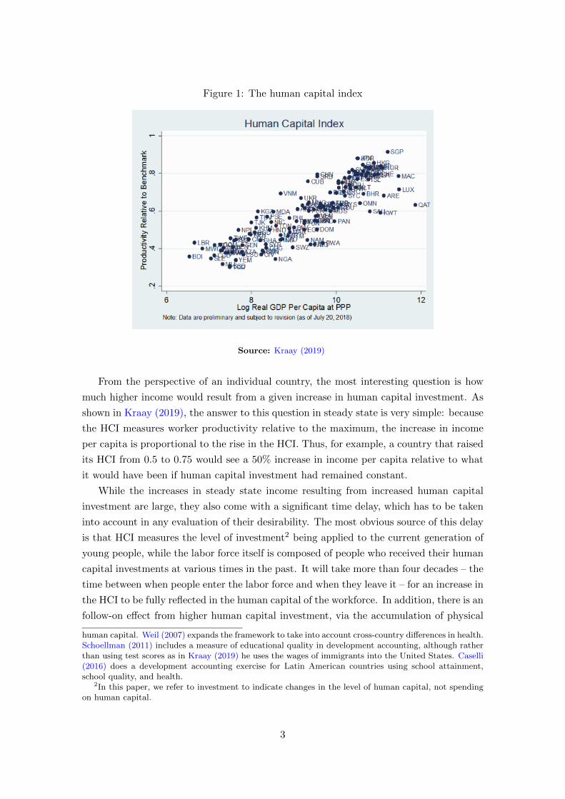
Figure 1: The human capital index

Source: Kraay (2019)

From the perspective of an individual country, the most interesting question is how

much higher income would result from a given increase in human capital investment. As

shown in Kraay (2019), the answer to this question in steady state is very simple: because

the HCI measures worker productivity relative to the maximum, the increase in income

per capita is proportional to the rise in the HCI. Thus, for example, a country that raised

its HCI from 0.5 to 0.75 would see a 50% increase in income per capita relative to what

it would have been if human capital investment had remained constant.

While the increases in steady state income resulting from increased human capital

investment are large, they also come with a significant time delay, which has to be taken

into account in any evaluation of their desirability. The most obvious source of this delay

is that HCI measures the level of investment2 being applied to the current generation of

young people, while the labor force itself is composed of people who received their human

capital investments at various times in the past. It will take more than four decades – the

time between when people enter the labor force and when they leave it – for an increase in

the HCI to be fully reflected in the human capital of the workforce. In addition, there is an

follow-on effect from higher human capital investment, via the accumulation of physical

human capital. Weil (2007) expands the framework to take into account cross-country differences in health.Schoellman (2011) includes a measure of educational quality in development accounting, although ratherthan using test scores as in Kraay (2019) he uses the wages of immigrants into the United States. Caselli(2016) does a development accounting exercise for Latin American countries using school attainment,school quality, and health.

2In this paper, we refer to investment to indicate changes in the level of human capital, not spendingon human capital.

3

capital, to higher output. This, too, takes time to fully play out. Assessing these effects

thus requires a more elaborate dynamic model, as in Ashraf, Lester, and Weil (2008).

Beyond tracking the evolution of GDP per capita in response to changes in HCI, we put

the model we construct to two additional uses. First, we extend the existing literature

by looking explicitly at how poverty rates evolve over time in response to changes in

HCI. Second, we use the model to compare changes in output and poverty generated by

changing HCI to those that would be generated by changes in the rate of investment in

physical capital.

Our starting point for this exercise is information on the demographic structure of the

population: how many people there are in each age group (specifically, we break down

the population into five-year age categories). The United Nations Population Division

collects this data, and also makes forecasts of demographic structure going forward, which

we incorporate into our model.

We combine this demographic data with information on the educational attainment

of the population, also broken down by five year age groups from Barro and Lee (2013),

augmented by IHME (2015). Having age-specific data on educational attainment is im-

portant because as time goes by, older cohorts, which tend to have lower educational

attainment, will be replaced in the labor force by younger, more educated cohorts, a

process that will automatically raise the average level of schooling in the population.3

Combining data on population age structure and educational attainment of different

age cohorts, we can calculate the average level of human capital per working age adult,

which is one of the inputs into production in the economy. We can also measure countries’

stocks of physical capital (the other key input into production). Within our model we

can track how the amount of physical capital evolves over time, under the assumption

that the investment rate stays fixed at is current level. With data on both human and

physical capital, as well as GDP per worker, we can also calculate a measure of total

factor productivity in every country. Finally, knowing the ratio of working age adults

to the population as a whole, we can track how production per worker is translated into

production per capita.

With all of these pieces in place, we can construct scenarios laying out how the stan-

dard of living in a country will change over time under different assumptions of the value

that HCI will take (that is, different assumptions as to how the human capital of the

youngest generation of workers evolves over time). Our particular interest is in how

changing the HCI from its current level will play out in terms of income and poverty. To

do this analysis, we start by constructing a baseline scenario of how the economy will

develop if the current level of HCI is maintained into the future. Along this baseline

path, growth and poverty reduction occur for four reasons. First, as mentioned above,

the current HCI in most countries represents a higher level of investment than was re-

3Ideally, we would like to have similar data on school quality and childhood health inputs by age cohort.Unfortunately, such data are not available.

4

ceived by older cohorts of workers. Thus the process of aging and labor force replacement

will naturally raise the average level of human capital per worker. Second, the ratio of

working age to total population is forecast to change in response to past (and forecast)

variations in fertility. In many developing countries, this “demographic dividend” will be

of significant magnitude. Third, we expect productivity to grow going into the future, as

it has historically.4 Finally, the level of physical capital will adjust, in particular growing

in most countries as productivity and human capital per worker increase.

Moving from forecasts of income per capita to forecasts of the poverty rate requires

some additional machinery. Poverty is a function of both the average level of income and

how income is distributed among households. For example, in a country where average

household income is above the poverty threshold, a higher level of income inequality will

imply that the fraction of households that are poor will be higher. Inequality is measured

by the Gini coefficient, for which the World Bank has an estimate for every country in

our sample. In forecasting future poverty, in both our baseline and alternative scenarios,

we assume that the Gini coefficient in each country remains constant at its most recently

observed level.

To assess the effect of increased HCI, we compare the changes in income and poverty

that would result from a particular policy (which we call an alternative scenario) to the

changes in those same measures that would occur in the baseline scenario just described.

Income rises and poverty falls in the baseline scenario. By looking at how the alternative

scenario differs from the baseline, we don’t inadvertently give credit to a particular policy

innovation for changes in income and poverty that would take place anyway.

We consider three alternative scenarios. As described in greater detail below, two of

these scenarios are based on data on how HCI levels have increased over the period 2005-

2015 in the subset of countries for which such data are available. The first observes how

the gap between the HCI and the maximum of 1.0 has changed for the median country in

our data. We then apply this rate of change in the gap to all countries in our simulation.

This corresponds to countries closing the gap between their current levels of HCI and

the maximum of 1.0 at a rate of approximately 4% every five years. In this scenario,

the typical developing country, with an HCI of 0.5 in 2015, would see this value rise to

around 0.62 in 2050. The second scenario more optimistically assigns to each country the

rate of improvement in each component that is the 75th percentile of what was observed,

which corresponds to a country closing 9% of the gap between its current HCI and the

4A potentially important omission in our model is any linkage between human capital accumulation andproductivity growth. In many endogenous growth models, human capital is the engine of growth, eitherbecause it endogenously grows itself (Lucas Jr 1988; Ehrlich and Kim 2007), because it speeds up thecreation of new technologies (Ehrlich 2007), or because it facilitates the import of cutting-edge technologyfrom abroad (Jones 2003). To the extent that any of these channels are operative, increased human capitalaccumulation will have a larger effect on growth than what we model. In the developing countries thatare our central concern in this paper, the third channel is probably the most relevant. Unfortunately, wedo not have good structural estimates of the role of human capital in facilitating technology transfer thatwe can apply.

5

maximum of 1.0 every five years.

To give a flavor of the results, we find that in the first of these alternative scenarios,

GDP per capita in the world as a whole would be 5% percent above its level in the

baseline scenario in the year 2050, and among the low and lower-middle income countries

(what we will call developing countries), the increase would be 9%. The poverty rate -

the percentage of those living on less than $1.90 a day - would similarly be 0.7 percentage

points lower by 2050 than it would along the baseline scenario (1.2 percentage points in

developing countries). Another way to assess effect of this policy is by looking at the

year by which a particular poverty target is reached. For example, for the policy just

described, developing countries as a whole would reach a 5% poverty rate between 2045

and 2050, as compared to between 2050 and 2055 in the baseline scenario.

In addition to the two scenarios just described, we also include results from a more

dramatic policy in which every country in the world were to instantaneously (as of the

year 2020) raise its level of HCI to the highest possible level, that is, 1.0 on the scale

described above. This scenario is not meant to be realistic, but rather included solely as

an aid to understanding the dynamics of the model. In this case, worldwide, the poverty

rate in the year 2050 would be 2.5 percentage points lower than it would be in the baseline

scenario.

Although focus on reporting results for large groups of countries, the model that we

have constructed in fact examines the data on a country-by-country basis. In this context,

it can be used for planning and assessment: What dividends will be reaped by a particular

increase in HCI, and when will they arrive? What path of changes in HCI is required to

hit a particular target?

Of course, the output of our simulation model, as with any such model, is subject to

a fair bit of uncertainty. Some of this uncertainty has to do with the baseline scenario

itself. We build into the baseline scenario assumptions about future demographic change,

the investment rate, and productivity growth, all of which might turn out to be wrong.

However, because our main interest is in evaluating the effects of particular policies, and

because our methodology compares alternative and baseline scenarios which use the same

assumptions about future values of these non-policy variables, errors in our forecasts

of these variables largely cancel out. A more serious source of potential error in our

assessment of policies is if we have not included all of the different pathways by which

HCI affects income growth and poverty.

One pathway that we do not include in the basic model of Sections 2-4 is the effect

of parental human capital on fertility and on children’s human capital investments. In

Section 5, we address this deficiency, integrating the results from our simulation with

existing estimates of the effect of education on fertility and of fertility on income, the

latter running through several different channels. We find that allowing for this additional

causal channel greatly amplifies the estimated impact of an initial increase in human

capital investment in raising income.

6

A second important pathway by which an increase in HCI would affect poverty is by

changing the distribution of income. In our simulations, we assume that that the level

of inequality in a country (the Gini coefficient) would be the same in the alternative

scenarios as in the baseline scenario. Realistically, however, increases in HCI are likely to

raise the human capital of poor people more than that of rich people, simply because the

former group has a much larger deficiency to be addressed. A more equal distribution of

human capital would in turn be expected to reduce inequality, and thus to reduce poverty

by even more than we are accounting for in our alternative scenarios.

The rest of this paper is organized as follows. Section 2 lays out our model, discusses

the underlying data, and describes the different scenarios we analyze. Section 3 presents

the simulated paths of income per capita and poverty in the different scenarios. In Section

4, we consider the relative efficacy of human capital investment and physical capital

investment for achieving a given increment to income growth. Section 5 discusses an

extension of the model to take into account the effect of higher human capital investment

on fertility, and of fertility on income and human capital investment. Section 6 concludes.

Appendix A.2 compares our findings to an alternative version of the model that includes

tertiary education, while Appendix A.1 describes comparability issues in mapping between

the Institute for Health Metrics and Evaluation (IHME) and Barro-Lee datasets.

2 Model Specification

In this section we describe in more detail the model we use to simulate the effects of

changes in human capital investment on economic growth and poverty reduction. The

model uses standard components. We assume output is produced in a Cobb-Douglas pro-

duction function using physical capital and quality-adjusted labor as inputs. The growth

rate of total factor productivity, representing technological change and the efficiency of

institutions, is taken as exogenous and constant. We also take forecast demographic

changes as exogenous and invariant to the changes in human capital investment that we

consider.

The innovations in the model come in the calculation of quality-adjusted labor input,

that is, in looking at the effect of human capital investments on how much labor workers

can supply. We follow the methodology and parametrization of Kraay (2019) in using

data on years of education, school quality, and health outcomes to construct measures

of human capital for new cohorts of workers, and then track the human capital of the

aggregate labor force as cohorts of new workers replace the older ones. As discussed in

more detail below, we also translate changes in output per worker into per-capita income

changes, and use these to track the effect of growth on poverty.

7

2.1 Basic Assumptions

Time, denoted as t, proceeds in five year increments. Our model will be calibrated for

2015, when t = 0, then t = 1 will indicate 2020, and so on.

While working ages can vary across contexts, in the model we treat all individuals

aged 20-64 as being members of the labor force. For many developing countries, fifteen

would be a more appropriate age for the start of labor force participation. However, the

education data we rely on includes schooling up through the 12th grade, which typically

ends at the age of eighteen. We thus begin the analysis at the age of twenty in order to

capture all gains in secondary school attainment measured in the Barro-Lee data. We

assume all individuals fully participate in the labor force during these ages, regardless

of gender or age. Furthermore, we do not make any adjustment for people being out of

the labor force while receiving education after the age of twenty, or for their being in the

labor force prior to this age.

We will denote population in five year age bins (20-24, 25-29...). Age is denoted a.

We will index age groups by the first age of the bin, i.e. a = 20, 25, etc.

Throughout the simulation, we take as given age-specific population totals by five year

age groups from World Population Prospects: the 2017 Revision’s medium variant esti-

mates (United Nations Department of Economic and Social Affairs, Population Division

2017). Population projections are treated as exogenous: we do not allow for feedback

from human capital (or income) to fertility, mortality, or labor force participation. We

also do not allow for differential mortality by education.

For education, we look only at data on attainment through secondary school. Our

primary reason for ignoring tertiary education is that available data on school quality

(discussed below) are only applicable to primary and secondary education. We were

not comfortable assuming that the measured differences apply to tertiary education. In

Appendix A.1, we extend the model to include tertiary education, and show that in fact

the predictions regarding the paths of income and poverty are very similar to those in our

main exercise.

In this paper, we assume that the level of human capital observed in 20-24 year olds

in 2015 corresponds to Human Capital Index: it measures the flow of human capital

investment. For example, if the HCI takes on a value of 0.75 for a country in 2015, we

assume this means that 20-24 year olds in that year will have a level of human capital

of 0.75 (even though the level of human capital for the rest of the workforce may be

different).

For the purpose of calculating changes in human capital, capital, productivity, GDP

and poverty, we will analyze countries individually. Later on, we will aggregate these

results to consider the effects for different country income groups or for the world. For

our calculations below, we will not use country subscripts.

8

2.2 Calibration for t = 0

For calibration the model for the first period, we rely on 2015 data where possible. When

it is not available we use the nearest available year. Below we describe how this data is

used to generate starting values for the model.

Population by age and Working Age Population

Let Pa,t be the number of individuals (combining both sexes) in age group a in year t.

We define the Working Age Population as

WrkAget =60∑

a=20

Pa,t (1)

And the fraction of the Working Age Population as

WrkAgeFractt =WrkAget∑

a Pa,t(2)

Gross Domestic Product

For GDP, we use the World Bank’s measure of GDP in 2015, measured in constant 2011

international dollars at purchasing power parity (PPP). Let this measure be GDP0. We

then defined GDP per worker as

GDPperWorker0 =GDP0

WrkAge0(3)

And GDP per capita as

GDPperCapita0 = GDPperWorker0 ×WrkAgeFract0 (4)

Physical Capital Stock

Total capital at time zero is defined as K0 . Our source is the Penn World Tables 9.0,

from which we use a country’s 2014 value of capital stock at current PPPs in millions of

2011 $US. We then define capital per worker as:

KperWorker0 =K0

WrkAge0(5)

Education Attainment

We obtain data on educational attainment each five year age group from two sources.

The first is Barro-Lee‘s database of educational attainment, which covers 146 countries

9

up to the year 2010, and is disaggregated both by sex and by five-year age groups (Barro

and Lee 2013).5

For our estimates of 2015 educational attainment, we assume each age group retains

the value it would have had five years previously - that no cohort obtains any further years

of schooling following 2010. For example, we assume the 35-39 age group has the same

educational attainment as the 30-34 age group did in 2010. As not everyone in the 2015

20-24 age group would have completed their secondary schooling in 2010, we assign the

2015 20-24 age group the same value as the 2010 20-24 age group. For the small subset of

countries that have combined primary and secondary schooling attainment greater than

12 years, we cap these values at 12.

Barro-Lee data is unavailable for 75 countries in our dataset. For these, we use data

on educational attainment from estimates produced by the Institute of Health Metrics

and Evaluation (IHME 2015). IHME’s data does not distinguish between different levels

of schooling. We convert IHME years of schooling into Barro-Lee Primary and Secondary

schooling equivalents using a method described in Appendix A.2. As with the Barro-Lee

data, we cap average years of schooling at 12 years.

Define EAa,t as the average number of years of primary plus secondary school of

individuals in age group a in year t. For the calculations below, we will take the theoretical

maximum of this measure to also be 12.6

Education Quality

Data on educational quality is more sparse than that on attainment. Where attainment

data is available for older cohorts, data on the quality of education covering all the age-bins

in our data is rarely available, particularly for developing countries infrequently subject

to testing.

We thus assume that all cohorts at time zero have the same quality of education, even

if they differ in their attainment, so that

EQa,0 = EQ0∀a (6)

EQ0 in each country is assigned based on data on the most recent available observation

of harmonized test scores from Altinok, Angrist, and Patrinos (2018). These are in “PISA-

equivalent units.” Defining the most recent test score as Score0, we convert it into a

quality measure using the methodology of Angrist, Filmer, Gatti, Rogers, and Sabarwal

(2018).

5It is worth noting that the World Bank’s version of the HCI uses expected years of schooling (EYS)as produced by UNESCO. We deviate from the WB methodology in this case as EYS is not broken ownby age groups, which is necessary for our simulation exercise.

6Note that this treatment of educational attainment differs from that in the Human Capital Index,which uses UNESCO methodology to calculate Expected Years of Schooling (EYS), based on a totalpotential 14 years of schooling pre-primary through 12th grade. To deal with that mismatch, in thesections below we will scale up educational attainment proportionally to the change in EYS.

10

EQ0 = 1−Ψ× (625− Score0

625) (7)

Where we set Ψ = 1, which is consistent with the findings of that paper.

Adjusted Years of Education and Human Capital from Education

Quality adjusted years of education for all age cohorts at time zero are calculated by

multiplying their years of schooling (adjusted as described above) by the time-zero quality

measure, specifically

AdjEda,0 = EAa,0 × EQ0 (8)

Finally, human capital from education (scaled to be 1 in the theoretical maximum

country) is constructed for each age group at time zero as

HCSchoola,0 = e(φ×(AdjEda,0−12)) (9)

Where φ is the Mincerian return to human capital, assumed to be .08.

Health and human capital from health

As with education quality, we are unable to separately determine the health status of

different age bins in our data. This would require finding childhood health inputs for

currently middle aged workers at the time when they were young. Instead, we rely on

the two contemporaneous health measures used in the HCI, the proportion of children

who are stunted and adult survival rates (ASR), and apply them to the entire adult

population. Our two input measures of health are ASRt and Stuntingt, where the latter

is not available for all countries.

Human capital from health is constructed directly from these measures. It is scaled

to have a value of 1 in a country with perfect health. If both measures are present, we

construct

HCHealtha,0 = e(γASR×(ASR0−1)−γStunting×Stunting0)

2 (10)

If only ASR data are available, then we construct health human capital from just

ASR, so that

HCHealtha,0 = e(γASR×(ASR0−1)) (11)

We use values of γASR = 0.6528 and γStunting = 0.3468 based on Weil (2007) and

Kraay (2019).

11

Total Human Capital

Total human capital for an age cohort is the product of human capital from schooling

and human capital from health

HCa,0 = HCSchoola,0 ×HCHealtha,0 (12)

Total human capital for the economy is simply the sum of cohort-specific human

capital multiplied by population. In practice, we only look at this in per worker terms:

HCperWorker0 =(∑60

a=20 Pa,0 ×HCa,0)WrkAge0

(13)

Productivity at t = 0

We calculate productivity in 2015 using our measures of GDP per worker, capital per

worker and human capital per worker.

A0 =GDPperWorker0

KperWorkerα0 ×HCperWorker(1−α)0

(14)

Where we take the base case value of α = 13

Poverty Headcount

Let Gini0 be the Gini coefficient at time zero (measured on a 0-1 scale). We assume that

income growth does not affect the Gini coefficient. Pov0 is the poverty headcount at time

zero (also measured as a fraction between zero and one).

We assume that household income is distributed lognormally, with µ and σ being the

mean and standard deviation of the log of income. The Gini coefficient is thus given by

Gini = 2× Φ( σ√

2

)− 1 (15)

Where Φ is the normal CDF. We then calculate the time zero standard deviation of the

log of income, which itself is constant as a result of the Gini being held constant.

σ = Φ−1(Gini0 + 1

2

)×√

2 (16)

Define P as the poverty threshold. The poverty headcount at time zero is given by

Pov0 = Φ( ln(P )− µ0

σ

)(17)

Rearranging,

µ0 = ln(P )− σ × Φ−1(Pov0) (18)

12

We calculate µt by assuming that the arithmetic mean level of household income has

grown by the same proportion as GDP per capita. Let mt be the arithmetic mean of

household income.

mt

m0=GDPperCapitatGDPperCapita0

(19)

From the property of the lognormal,

mt = e(µt+σ2

2)

Thus

ln(m0) = µ0 +σ2

2

ln(mt) = µt +σ2

2

So

µt = µ0 + ln(GDPPerCapitatGDPPerCapita0

)(20)

The expression for the poverty headcount at time t is:

Povt = Φ( ln(P )− µt

σ

)

Substituting in the expressions for µ0 and µt above, we calculate the poverty rate at

time t as

Povt = Φ[Φ−1(Pov0)− (

1

σ)ln(GDPPerCapitatGDPPerCapita0

)](21)

We perform these calculations for all three prevailing poverty lines: $1.90, $3.20 and

$5.50 a day PPP. Data on poverty headcount ratios and Gini coefficients for each country

are taken from the most recent year available from the World Bank’s data (produced by

PovCal).

13

Investment Rate

For the investment rate Inv0, we rely on the World Bank’s measure of gross capital

formation as a percentage of GDP. We assume the investment rate remains constant

throughout the entire scenario, and takes on the value of each country’s average over the

years 2006-2015.

2.3 Simulation Scenarios

For each country we have data for, we will construct several scenarios, each of which will

be derived from the time paths followed by all of the endogenous variables. Each scenario

will share a common rate of productivity growth, which will be taken as exogenous:

At = A0(1 + g)5t (22)

We will set g = .013, which is chosen so that the world poverty rate in 2030 is equal

to 5.6% in the “typical” scenario that we discuss below. The value of 5.6% is consistent

with World Bank forecasts of poverty in that year.

Baseline Scenario (Constant HCI)

We will start by constructing a path that would be followed if the investments in human

capital per worker remained constant at its time zero level (the current HCI). That is,

the human capital of the youngest working generation (those aged 20-24) stays fixed,

and slowly the entire population takes on that same value as older generations age out

of the workforce. Additional dynamics will come from productivity growth, physical

capital accumulation, change in the size of the working age population, and change in the

dependency ratio.

Cohort specific human capital is constructed by “aging” all existing working age co-

horts, and then assigning to the youngest working age cohort the level of human capital

from the youngest cohort at time zero.

HC20,t+1 = HC20,0

HCa+5,t+1 = HCa,t for a = 25 . . . 60

HCperWorkert =(∑60

a=20 Pa,t ×HCa,t)WrkAget

(23)

Capital evolves as follows:

14

KperWorkert+1 =WrkAgetWrkAget+1

[KperWorkert+5×(Inv0AtKperWorkerαt HCperWorker1−αt −δkt)]

(24)

We use a base case value of δ = .05 for capital depreciation. GDP per worker and

GDP per capita are then generated as

GDPperWorkert = At ×KperWorkerαt ×HCperWorker1−αt (25)

GDPperCapitat = GDPperWorkert ×WrkAgeFract (26)

The baseline scenario is useful for understanding how, even when human capital in-

vestments remain fixed, GDP per capita and poverty would evolve solely due to older

cohorts with lower levels of educational attainment ageing out of the workforce. We next

consider three alternative scenarios where the entire HCI, the human capital of workers

age 20-24, rises at different rates over the 25 years, with varying degrees of optimism.

Scenario 1: Typical growth in the HCI

We first consider the scenario where countries experience increases in the components of

human capital at the same rate as the median country did over the past decade. For this,

we turn to the data underlying the World Bank’s HCI on expected years of schooling,

harmonized learning outcomes, stunting rates and adult survival rates. For the countries

that there is data for both 2005 and 2015, Table 1 displays the rate of change at the 50th

percentile for each outcome separately.

We consider the collective effect of these changes at the 50th percentile would have

on the HCI of a country with median levels of these outcomes as measured in the latest

version of the HCI in 2017. That is, what the change in the HCI would be if a country

with EYS of 11.78, harmonized learning outcomes of 423.57, non-stunted rates of 0.77,

and adult survival rates of 0.87 increased these outcomes by 0.474, 6, 0.051 and 0.022

respectively.

Specifically, we consider the percentage change in the “HCI gap,” the difference be-

tween the average human capital of the first age bin and the theoretical maximum of 1.0,

that would result from this “typical” increase in the components. Define Closedt as the

fraction in the gap between the time zero value of the HCI and its maximum that has

been closed in year t. A value of zero indicates that the country has not changed its HCI

since time zero. A value of one indicates that it has moved all of the way to maximum

level of HCI.

15

Table 1: Typical and optimistic values for changes in human capital

OutcomeChange between 2005-2015

Median value in 201750th percentile 75th percentile

Expected years of schooling 0.474 1.131 11.78Harmonized learning outcomes 6 19 423.57(Non) stunting rates 0.051 0.1 0.77Adult Survival Rates 0.022 0.043 0.87

If a country with median values of the components saw the same increases in those

components as the 50th percentile country (for each component) did between 2005-2015,

we would expect that country to close roughly 1% (.0072) of the HCI gap every year, or

roughly 4% (.0353) every five years.

To simulate this scenario, rather than simulate changes in all the components of human

capital, we will instead apply a 4% (.0353) percentage decrease in the HCI gap for each

country every five years. Thus value of Closedt determines the human capital of the

youngest generation of workers, so that7

HC20,t = 1− Closedt × (1−HC20,0)

The implication of applying a uniform percentage decrease in the HCI gap is that coun-

tries with lower levels of the HCI will face higher levels of subsequent growth. For example,

low income countries, on average, have starting levels of human capital HC20,2015 = 0.43,

but see an increase by 0.0201 in the first five years. By contrast, upper middle countries

have on average HC20,2015 = 0.63, but only see an increase of 0.013 in the first five years.

Scenario 2: Optimistic Growth in the HCI

For our second scenario, we repeat the same exercise as in Scenario 1, but instead we

consider the percentage change in the HCI gap that would result from a country experi-

encing the same increase in the HCI components as countries at the 75th percentile do.

In this scenario, our hypothetical country would experience a 2% (.019) annual decrease

in the HCI gap, equivalent to approximately a 9% (.0914) decrease every five years. We

take this decrease as our optimistic scenario, and thus apply a 9% decrease in the HCI

gap for each country in our simulation every five years.

7Note that we assume that future improvements in human capital investment only affect new cohortsof workers. This assumption is clearly appropriate in the cases where the improvement takes the form ofhigher school quality and additional years of primary and secondary education. In the case of health, itis less clear. Improved health in the form of lower stunting clearly only affects children, but to the extentthat better health is reflected in adult survival, it may indicate both more human capital investmentin current young people and better health of current adults. By omitting this latter channel, we mayunderstate the effect of health improvements on output growth and poverty reduction.

16

Scenario 3: the HCI moves to the frontier immediately

In this scenario, we consider the change in GDP per capita and poverty that would result

from each country immediately moving to the frontier - an HCI of 1.0. In this scenario,

each new 20-24 age group has human capital per worker of one, and the human capital

per worker across the entire workforce slowly converges to this value as the older cohorts

age out of the workforce.

While this is clearly not a plausible scenario for most countries, it is a useful exercise as

it establishes an “upper bound” for the growth effects of improvements in human capital,

as the growth effects of investments today only manifest as quickly as the workforce ages

and is replaced.

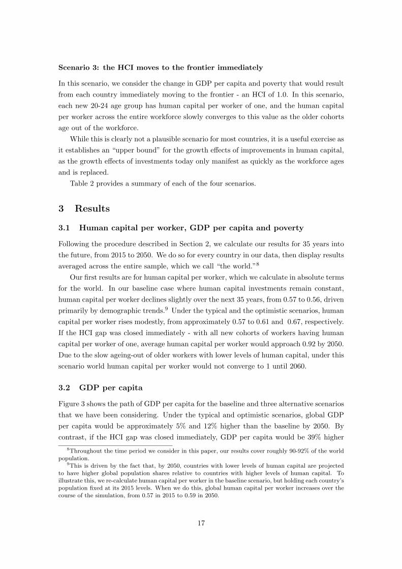
Table 2 provides a summary of each of the four scenarios.

3 Results

3.1 Human capital per worker, GDP per capita and poverty

Following the procedure described in Section 2, we calculate our results for 35 years into

the future, from 2015 to 2050. We do so for every country in our data, then display results

averaged across the entire sample, which we call “the world.”8

Our first results are for human capital per worker, which we calculate in absolute terms

for the world. In our baseline case where human capital investments remain constant,

human capital per worker declines slightly over the next 35 years, from 0.57 to 0.56, driven

primarily by demographic trends.9 Under the typical and the optimistic scenarios, human

capital per worker rises modestly, from approximately 0.57 to 0.61 and 0.67, respectively.

If the HCI gap was closed immediately - with all new cohorts of workers having human

capital per worker of one, average human capital per worker would approach 0.92 by 2050.

Due to the slow ageing-out of older workers with lower levels of human capital, under this

scenario world human capital per worker would not converge to 1 until 2060.

3.2 GDP per capita

Figure 3 shows the path of GDP per capita for the baseline and three alternative scenarios

that we have been considering. Under the typical and optimistic scenarios, global GDP

per capita would be approximately 5% and 12% higher than the baseline by 2050. By

contrast, if the HCI gap was closed immediately, GDP per capita would be 39% higher

8Throughout the time period we consider in this paper, our results cover roughly 90-92% of the worldpopulation.

9This is driven by the fact that, by 2050, countries with lower levels of human capital are projectedto have higher global population shares relative to countries with higher levels of human capital. Toillustrate this, we re-calculate human capital per worker in the baseline scenario, but holding each country’spopulation fixed at its 2015 levels. When we do this, global human capital per worker increases over thecourse of the simulation, from 0.57 in 2015 to 0.59 in 2050.

17

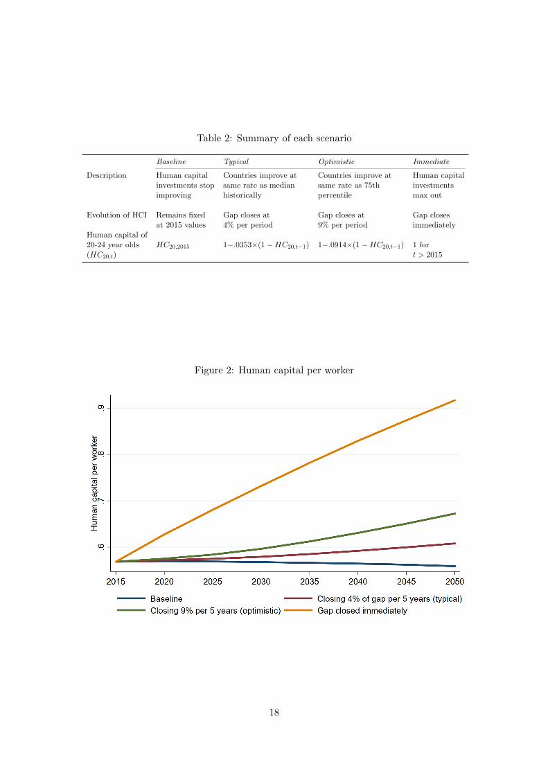
Table 2: Summary of each scenario

Baseline Typical Optimistic Immediate

Description Human capital Countries improve at Countries improve at Human capitalinvestments stop same rate as median same rate as 75th investmentsimproving historically percentile max out

Evolution of HCI Remains fixed Gap closes at Gap closes at Gap closesat 2015 values 4% per period 9% per period immediately

Human capital of20-24 year olds HC20,2015 1−.0353×(1−HC20,t−1) 1−.0914×(1−HC20,t−1) 1 for(HC20,t) t > 2015

Figure 2: Human capital per worker

18

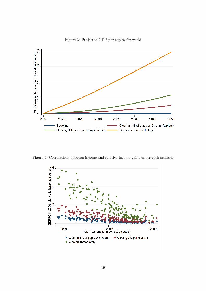
Figure 3: Projected GDP per capita for world

Figure 4: Correlations between income and relative income gains under each scenario

19

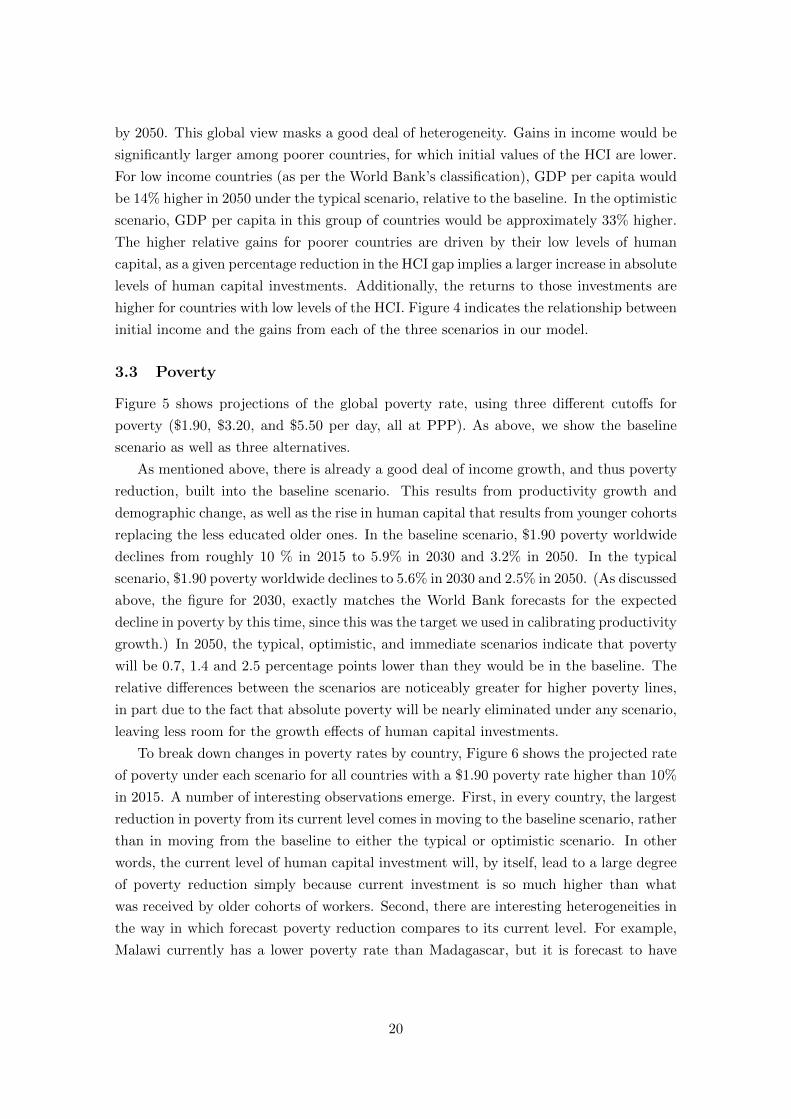
by 2050. This global view masks a good deal of heterogeneity. Gains in income would be

significantly larger among poorer countries, for which initial values of the HCI are lower.

For low income countries (as per the World Bank’s classification), GDP per capita would

be 14% higher in 2050 under the typical scenario, relative to the baseline. In the optimistic

scenario, GDP per capita in this group of countries would be approximately 33% higher.

The higher relative gains for poorer countries are driven by their low levels of human

capital, as a given percentage reduction in the HCI gap implies a larger increase in absolute

levels of human capital investments. Additionally, the returns to those investments are

higher for countries with low levels of the HCI. Figure 4 indicates the relationship between

initial income and the gains from each of the three scenarios in our model.

3.3 Poverty

Figure 5 shows projections of the global poverty rate, using three different cutoffs for

poverty ($1.90, $3.20, and $5.50 per day, all at PPP). As above, we show the baseline

scenario as well as three alternatives.

As mentioned above, there is already a good deal of income growth, and thus poverty

reduction, built into the baseline scenario. This results from productivity growth and

demographic change, as well as the rise in human capital that results from younger cohorts

replacing the less educated older ones. In the baseline scenario, $1.90 poverty worldwide

declines from roughly 10 % in 2015 to 5.9% in 2030 and 3.2% in 2050. In the typical

scenario, $1.90 poverty worldwide declines to 5.6% in 2030 and 2.5% in 2050. (As discussed

above, the figure for 2030, exactly matches the World Bank forecasts for the expected

decline in poverty by this time, since this was the target we used in calibrating productivity

growth.) In 2050, the typical, optimistic, and immediate scenarios indicate that poverty

will be 0.7, 1.4 and 2.5 percentage points lower than they would be in the baseline. The

relative differences between the scenarios are noticeably greater for higher poverty lines,

in part due to the fact that absolute poverty will be nearly eliminated under any scenario,

leaving less room for the growth effects of human capital investments.

To break down changes in poverty rates by country, Figure 6 shows the projected rate

of poverty under each scenario for all countries with a $1.90 poverty rate higher than 10%

in 2015. A number of interesting observations emerge. First, in every country, the largest

reduction in poverty from its current level comes in moving to the baseline scenario, rather

than in moving from the baseline to either the typical or optimistic scenario. In other

words, the current level of human capital investment will, by itself, lead to a large degree

of poverty reduction simply because current investment is so much higher than what

was received by older cohorts of workers. Second, there are interesting heterogeneities in

the way in which forecast poverty reduction compares to its current level. For example,

Malawi currently has a lower poverty rate than Madagascar, but it is forecast to have

20

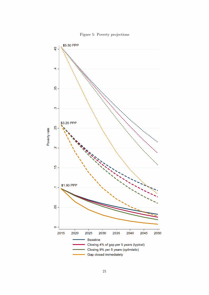
Figure 5: Poverty projections

21

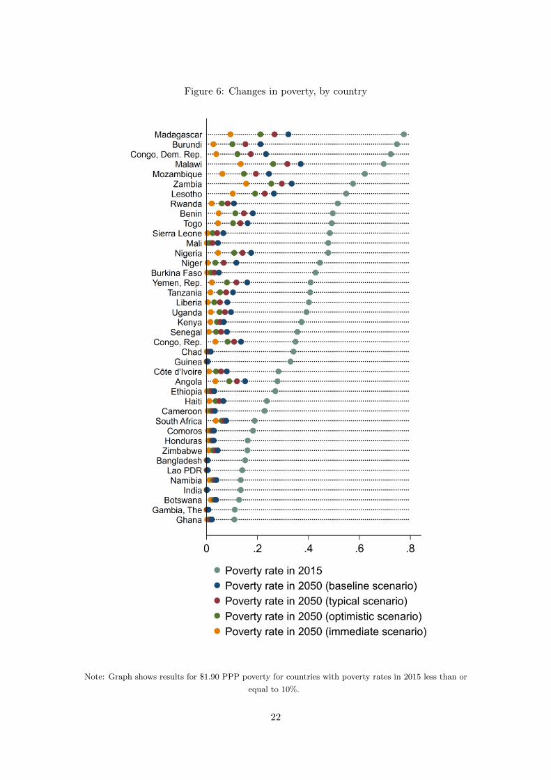
Figure 6: Changes in poverty, by country

Note: Graph shows results for $1.90 PPP poverty for countries with poverty rates in 2015 less than or

equal to 10%.

22

Figure 7: Number of people not in poverty, relative to baseline

23

higher poverty than that country in 2050 in each of the scenarios that we consider.10

In Figure 7 we consider the number of people who would have been poor in the baseline

scenario, but are not in our other three scenarios. Under the optimistic scenario, roughly

130, 300 or 540 million fewer people will be in poverty by 2050 than would have otherwise

been under the $1.90, $3.20 and $5.50 poverty lines respectively.

4 Human Capital vs. Physical Capital Investments

Throughout this paper we have been examining the potential for increased investment in

human capital, as captured by the HCI, to raise economic growth and reduce poverty.

Naturally, before endorsing such a policy it would be useful to compare its cost/benefit

ratio with alternatives. The most natural of these to consider is investment in physical

capital. A full comparison is beyond the scope of the current paper, because we have

not in fact specified the costs of raising HCI. To cast some illumination on the issue, we

proceed along a different track, which is to compare the magnitude of increases in HCI

and in physical capital that would be required to achieve a specific increase in output (and

reduction in poverty) in the steady state. We can also use our dynamic model to examine

the time paths of output and poverty in response to these two different interventions.

To be concrete, we consider a specific country, Cambodia. In 2015, the value of human

capital per worker among 20-24 year olds was 0.488. The physical capital investment rate

averaged over 2006-15 was 20.1%. Consider now the effect of raising human capital

investment such that the HCI gap closes by 3.5%, as occurs in the first five-year period

of the typical scenario. For simplicity, we consider only this one time change, rather

than looking at a full path of changes in HCI. The 3.5% decrease in the gap means that

investment rate for new workers will rise from 0.488 to 0.506, an increase of 3.7%. It is

easy to show that an increase in human capital investment of this magnitude would raise

GDP per capita by 3.7% in steady state.

We now ask what increase in physical capital investment would be required to achieve

the same steady state increase in income. In the Solow model, steady state output per

capita is proportional to the investment rate raised to the power α1−α . Using a value of

one-third for α , this implies that raising steady state GDP per capita by a factor of

1.0371 would require the investment rate of increase by a factor of 1.03712 = 1.0755. In

the case of Cambodia, this would mean raising the investment rate from 20.1% to 21.6%,

or 1.5 percentage points.

While the two changes in policy just considered would have the same steady state

effects, the transitions to the steady state would be different. Put differently, both human

capital and physical capital investments take time to fully bear fruit, but the time profiles

10It is worth remembering that these projections come from a simplified model that we are using toanalyze a set of stylized scenarios. They are not necessarily comparable with long-run poverty forecastsproduced by the World Bank.

24

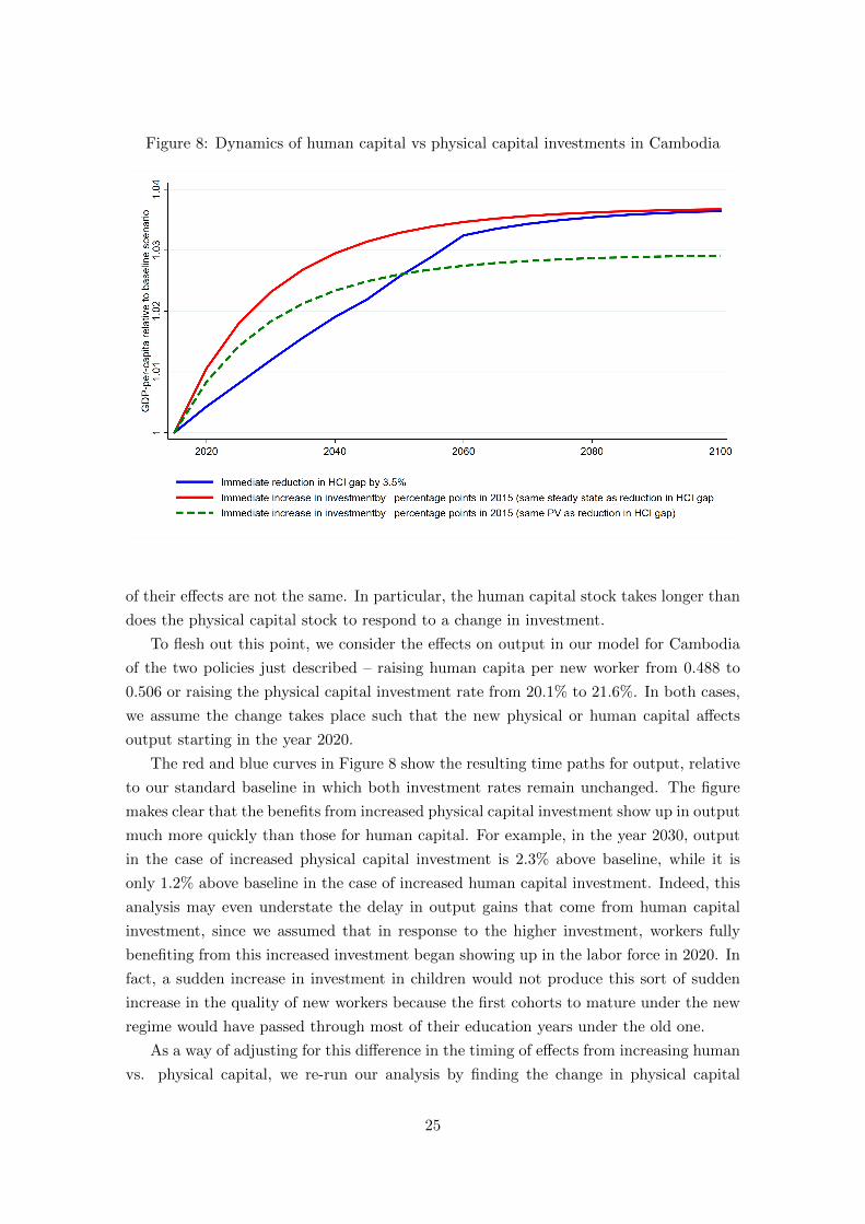
Figure 8: Dynamics of human capital vs physical capital investments in Cambodia

of their effects are not the same. In particular, the human capital stock takes longer than

does the physical capital stock to respond to a change in investment.

To flesh out this point, we consider the effects on output in our model for Cambodia

of the two policies just described – raising human capita per new worker from 0.488 to

0.506 or raising the physical capital investment rate from 20.1% to 21.6%. In both cases,

we assume the change takes place such that the new physical or human capital affects

output starting in the year 2020.

The red and blue curves in Figure 8 show the resulting time paths for output, relative

to our standard baseline in which both investment rates remain unchanged. The figure

makes clear that the benefits from increased physical capital investment show up in output

much more quickly than those for human capital. For example, in the year 2030, output

in the case of increased physical capital investment is 2.3% above baseline, while it is

only 1.2% above baseline in the case of increased human capital investment. Indeed, this

analysis may even understate the delay in output gains that come from human capital

investment, since we assumed that in response to the higher investment, workers fully

benefiting from this increased investment began showing up in the labor force in 2020. In

fact, a sudden increase in investment in children would not produce this sort of sudden

increase in the quality of new workers because the first cohorts to mature under the new

regime would have passed through most of their education years under the old one.

As a way of adjusting for this difference in the timing of effects from increasing human

vs. physical capital, we re-run our analysis by finding the change in physical capital

25

investment that would produce the same present value of output increases as the change

in human capital investment that we already specified. We use a 4% per year time

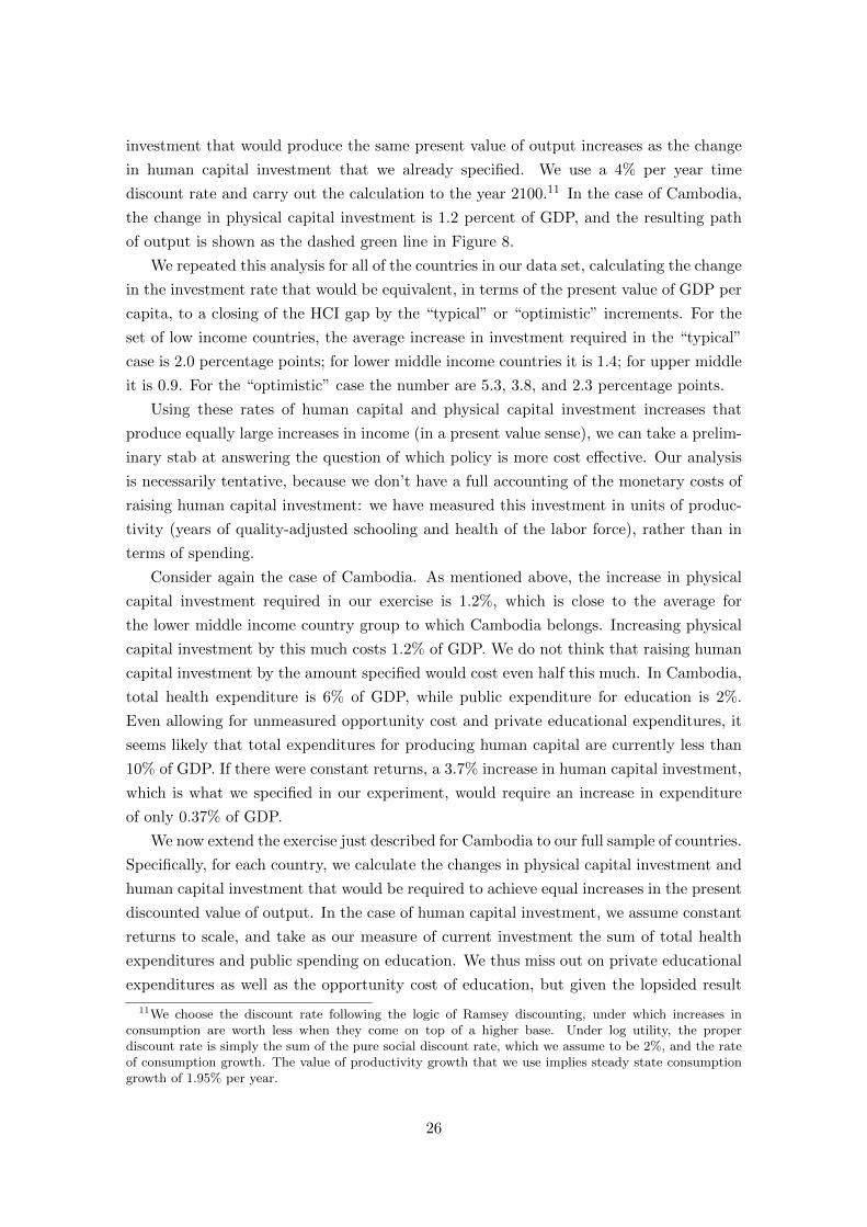
discount rate and carry out the calculation to the year 2100.11 In the case of Cambodia,

the change in physical capital investment is 1.2 percent of GDP, and the resulting path

of output is shown as the dashed green line in Figure 8.

We repeated this analysis for all of the countries in our data set, calculating the change

in the investment rate that would be equivalent, in terms of the present value of GDP per

capita, to a closing of the HCI gap by the “typical” or “optimistic” increments. For the

set of low income countries, the average increase in investment required in the “typical”

case is 2.0 percentage points; for lower middle income countries it is 1.4; for upper middle

it is 0.9. For the “optimistic” case the number are 5.3, 3.8, and 2.3 percentage points.

Using these rates of human capital and physical capital investment increases that

produce equally large increases in income (in a present value sense), we can take a prelim-

inary stab at answering the question of which policy is more cost effective. Our analysis

is necessarily tentative, because we don’t have a full accounting of the monetary costs of

raising human capital investment: we have measured this investment in units of produc-

tivity (years of quality-adjusted schooling and health of the labor force), rather than in

terms of spending.

Consider again the case of Cambodia. As mentioned above, the increase in physical

capital investment required in our exercise is 1.2%, which is close to the average for

the lower middle income country group to which Cambodia belongs. Increasing physical

capital investment by this much costs 1.2% of GDP. We do not think that raising human

capital investment by the amount specified would cost even half this much. In Cambodia,

total health expenditure is 6% of GDP, while public expenditure for education is 2%.

Even allowing for unmeasured opportunity cost and private educational expenditures, it

seems likely that total expenditures for producing human capital are currently less than

10% of GDP. If there were constant returns, a 3.7% increase in human capital investment,

which is what we specified in our experiment, would require an increase in expenditure

of only 0.37% of GDP.

We now extend the exercise just described for Cambodia to our full sample of countries.

Specifically, for each country, we calculate the changes in physical capital investment and

human capital investment that would be required to achieve equal increases in the present

discounted value of output. In the case of human capital investment, we assume constant

returns to scale, and take as our measure of current investment the sum of total health

expenditures and public spending on education. We thus miss out on private educational

expenditures as well as the opportunity cost of education, but given the lopsided result

11We choose the discount rate following the logic of Ramsey discounting, under which increases inconsumption are worth less when they come on top of a higher base. Under log utility, the properdiscount rate is simply the sum of the pure social discount rate, which we assume to be 2%, and the rateof consumption growth. The value of productivity growth that we use implies steady state consumptiongrowth of 1.95% per year.

26

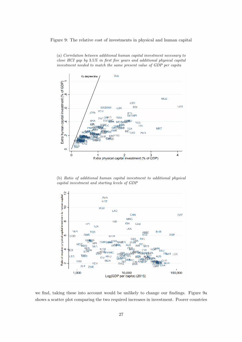
Figure 9: The relative cost of investments in physical and human capital

(a) Correlation between additional human capital investment necessary toclose HCI gap by 3.5% in first five years and additional physical capitalinvestment needed to match the same present value of GDP per capita

(b) Ratio of additional human capital investment to additional physicalcapital investment and starting levels of GDP

we find, taking these into account would be unlikely to change our findings. Figure 9a

shows a scatter plot comparing the two required increases in investment. Poorer countries

27

in general have higher required investment increases in either physical or human capital

in order to reach the target that we have specified. This is because the target involves

closing a fixed proportion of the gap in human capital relative to full investment, and

this gap is bigger in poorer countries. But it is notable that all of the data points in

the figure lie to the right of the 45-degree line, which is to say that in all countries the

required increase in physical capital investment is larger than the required increase in

human capital investment. Figure 9b shows the ratio of required investment in physical

capital to required investment in human capital on the vertical axis, and current GDP

per capita on the horizontal. There is a slight tendency for this ratio to be higher in

richer countries, but the more striking fact in the picture is that the ratio is high in all

the countries in the sample, generally ranging between two and six

5 Additional Causal Channels and General Equilibrium Ef-

fects

In the paper thus far we have considered the effect of an increase in human capital invest-

ment on income and poverty by focusing solely on the productive effects of that human

capital, that is, the extra output that will be produced by higher quality workers. Im-

plicitly, we ignore other potentially important channels by which human capital might

impact income and poverty, such as via an effect on fertility. We similarly ignore general

equilibrium effects, for example how higher income produced by an increase in human

capital will affect both fertility and future human capital accumulation, and similarly

how lower fertility will affect human capital accumulation. Our proceeding in this fash-

ion is determined primarily by the limitations on available estimates of the underlying

causal relationships among these endogenous variables. In the case of human capital’s

effect on productivity, we were able to take advantage of existing estimates of structural

parameters. But these are largely absent for other causal channels.

In some cases, we can speculate with reasonable confidence about the direction in

which consideration of general equilibrium effects would alter our findings. For example,

it is very likely that higher income would raise investment in human capital.12 Thus an

initial increase in the human capital investment, which our exercise shows would raise

income, would in turn feed back to even more human capital investment. In other words,

our exercise would understate the full effect of an initial policy-driven rise in HCI. In

other cases – for example, the structural effect of income on fertility – the sign of the

effect is not clear a priori.

In this section, we pursue one additional channel where we are able to get well identified

structural estimates, and which seems likely to be among the more important channels

12One channel would be by loosening the budget constraint for households and governments. Addi-tionally, we would expect capital accumulation from higher income to raise the return to educationalinvestments.

28

omitted in our analysis. This is the effect of increased human capital on fertility and

the follow-on effects of fertility on both income per capita and human capital investment.

The negative correlation between fertility and education (particularly female education)

is well known, but simply looking at this correlation does not immediately provide an

estimate of the structural effect of education on fertility. Following Karra, Canning, and

Wilde (2017), we use the estimate in Osili and Long (2008), derived from examining the

impact of a universal primary education program in Nigeria. Osili and Long find that an

extra year of education reduced fertility by 11%.13

Mapping this structural estimate into our framework requires taking a stand on

whether the effect of increased quantity of schooling on fertility (which is what they

measure) is the same as the effects of increasing other dimensions of human capital that

are included in the HDI, specifically school quality and health. Existing literature does

not give any guidance on this issue. We assume that indeed the effect of increasing either

of these other dimensions is the same as the effect of increasing school years.14

To get an estimate of the effect of human capital increases on fertility, we start with

the estimate from Osili and Long:

δln(f)

δs= −0.11 (27)

Similarly from the assumption that the Mincerian return to schooling is 8%, we have

δln(h)

δs= 0.08 (28)

Combining these two expressions, the elasticity of fertility with respect to human

capital (for changes in human capital that result from schooling) is -0.11/0.08 = -1.38.

We can apply this elasticity to the changes in human capital investment that we

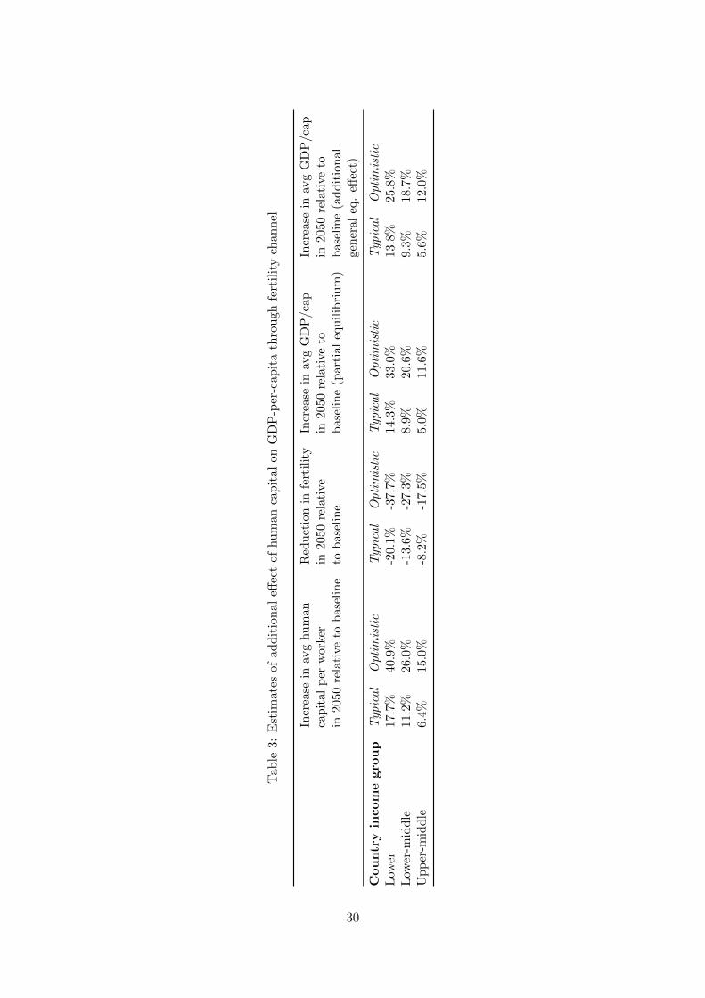
examine in the earlier in the paper. The first two columns of Table 3 show the increase

in human capital per worker in the year 2050 under the typical and optimistic scenarios,

each relative to the baseline, broken down into three country-income groups (we focus

on lower and middle income countries because we expect that the economic effects of

fertility reduction on income will be very different in upper income countries). Applying

the estimates just derived, we can convert these into implied reductions in fertility relative

to the baseline in each of these cases, as shown in the third and fourth columns of the

table.

The second step is to look at the effect of this reduction in fertility on income and

human capital investment. Doing this in a fully dynamic fashion would require a major

13In the paper, fertility in the treated cohort is only measured to age 25. The authors point to thestrong correlation between early and total fertility among non-treated cohorts to argue that the estimatecan be generalized to lifetime fertility. However, to the extent that higher educational attainment leadsto a delay rather than a reduction in lifetime fertility, their result may be overstated.

14If we assumed instead that raising years of schooling affected fertility while increasing school qualityand health did not, we would find a lower effect of higher HCI on fertility.

29

Tab

le3:

Est

imat

esof

add

itio

nal

effec

tof

hu

man

cap

ital

onG

DP

-per

-cap

ita

thro

ugh

fert

ilit

ych

an

nel

Incr

ease

inav

ghum

anR

educt

ion

infe

rtilit

yIn

crea

sein

avg

GD

P/c

apIn

crea

sein

avg

GD

P/ca

pca

pit

alp

erw

orke

rin

2050

rela

tive

in20

50re

lati

veto

in20

50re

lati

veto

in20

50re

lati

veto

base

line

tobas

elin

ebas

elin

e(p

arti

aleq

uilib

rium

)base

line

(addit

ional

gener

aleq

.eff

ect)

Cou

ntr

yin

com

egro

up

Typ

ical

Opti

mis

tic

Typ

ical

Opti

mis

tic

Typ

ical

Opti

mis

tic

Typ

ical

Opti

mis

tic

Low

er17.

7%40

.9%

-20.

1%-3

7.7%

14.3

%33

.0%

13.8

%25

.8%

Low

er-m

iddle

11.2

%26

.0%

-13.

6%-2

7.3%

8.9%

20.

6%9.

3%

18.

7%U

pp

er-m

iddle

6.4%

15.0

%-8

.2%

-17.

5%5.

0%11.

6%5.

6%

12.

0%

30

redesign of the model in the paper. That is because, comparing our baseline to the

different alternative paths, education is varying on a cohort-by-cohort basis, and we would

have to correspondingly adjust the age-specific fertility of each cohort to generate new

path of population.

As an alternative, we build off results from an existing macro-demographic model,

that of Ashraf, Weil, and Wilde (2013). That paper considers the effects of exogenous

reductions in the total fertility rate (TFR) in a model parameterized to match data

from Nigeria, which is classified by the World Bank as a lower middle income country.

Channels of causation that are modeled (based on well-identified microeconomic evidence)

include the effects of lower fertility on the dependency ratio, human capital investment,

female labor force participation, child health, and life cycle saving. The specific reduction

in fertility considered is from the United Nations medium variant forecast to the low

variance forecast. Although the simulation shows the value of income in each five year

period, we focus on the 50-year horizon presented in the paper, which corresponds to the

years 2060-64. In that period, the TFR is 2.87 under the medium variant forecast and

2.37 under the low variant – a reduction of 17.4% The corresponding increase in income

per capita comparing the low to the medium variant is 11.9%.15 In the seventh and eighth

columns of the table, we apply this same ratio of income changes to TFR changes to the

fertility changes that we just derived. For comparison, we also show (in columns five and

6) the direct effect of increased human capital on income per capita that come from our

model.

As the table shows, the additional general equilibrium effect resulting from reduced

fertility is quantitatively quite significant – indeed, looking across the different country

groups, in both the typical and optimistic scenarios, it is almost exactly the same magni-

tude (and always the same sign) as the direct productive effect of human capital on which

we have focused. While we think that this is potentially an important result, we suggest

that it should be taken with a grain of salt. First, as noted above, in tailoring results from

existing literature to the question at hand, we had to make several strong assumptions,

in which we erred in the direction that would have produced a larger effect. Second, we

were not able to fully dynamically look at the effect of human capital on fertility on a

cohort-by-cohort basis. Instead we had to take several shortcuts. This appears to be an

area in which future work could do a better job.

Despite the above-listed shortcomings, the exercise in this section can be used to add

some further nuance to results from Section 4. There, we found that, at the margin,

devoting an additional percentage of GDP to human capital produced a higher present

discounted value of income grains than devoting the same percentage of GDP to physical

capital investment. Existing literature has not identified the sorts of additional causal

channels from physical capital to income, beyond the direct productivity effect, that we

15Ashraf, Weil, and Wilde report that the largest contributor to this increase in income per capita,accounting for 40% of the total, is the reduction in the dependency ratio.

31

have discussed in the case of human capital. Thus properly taking into these channels

would certainly amplify the higher efficacy of human vs. physical capital investment.

6 Conclusion

Gaps among countries in the rate at which they invest in the human capital of their

citizens are large. Taking a broad measure that includes quality and quantity of education

as well as measures of the effect of health on worker productivity, there is a gap ranging

as high as a factor of three between the human capital of new workers in high investing

countries relative to those that invest the least. Investment rates in human capital are

highly correlated with income per capita, and indeed, the lower labor input of workers,

due to their health and education deficiencies, is an important contributor to the poverty

of many countries.

These observations suggest that raising investment in human capital represents an

attractive policy for increasing income and reducing poverty. In this paper we have

quantitatively explored the dynamic responses of income and poverty to such increased

investment. Consideration of the time dimension is particularly important in this case

because the benefits of higher human capital investment have very long gestation periods:

it takes a long time to produce a new worker, and an even longer time before existing

workers, who were subject to lower human capital investments during their youth, cycle

out of the labor force.

Our main exercise compared the paths of income and poverty that would be experi-

enced under two specified scenarios to those experienced on a baseline in which the rate

of human capital investment currently observed in every country remains constant into

the future. In one scenario (labelled “typical”), each country experiences a rate of growth

of human capital investment that is typical of what was observed in the decade ending in

2015. In this scenario, world GDP per capita is 5% higher than baseline in the year 2050,

while the global rate of $1.90 poverty is 0.7 percentage points lower in that same year.

In the “optimistic” scenario, in which each country is assumed to raise the components

of human capital investment at a rate corresponding to the 75th percentile of what was

observed in the data, world GDP per capita is 12% higher than baseline in 2050, while

the rate of $1.90 poverty drops by 1.4 percentage points. Under the optimistic scenario,

roughly 130, 300 or 540 million fewer people will be in poverty by 2050 than would have

otherwise been under the $1.90, $3.20 and $5.50 poverty lines respectively.

The increase in incomes and declines in poverty that would be observed in developing

countries are significantly larger than the world averages, because these countries are

faced with much larger gaps between their current investment rates and the level that

would represent full investment in the next generation. For example, among low income

countries (using the World Bank classification), GDP per capita would be 12% higher in

the “typical” scenario and nearly 25% higher in the “optimistic” scenario in the year 2050

32

than in the baseline.

We also used our model to compare the dynamics of output growth in response to

higher human capital investment to those resulting from higher investment in physical

capital. The latter delivers its growth benefits much more quickly – that is, a country can

build more machines and infrastructure at a faster pace than it can build better workers.

That being said, our informal comparison of the costs of the two types of investments sug-

gests that investing in people is sufficiently cheap in comparison to investing in machines

to overcome the timing advantage associated with investing in machines.

Although our analysis includes some of the channels by which higher human capital

would raise income, for example, by inducing the accumulation of more physical capital,

we also leave out some potentially important mechanisms. While we do not have the

structural estimates of causal effects that would allow us to explore all of the possible

additional channels and general equilibrium effects resulting from an increase in human

capital investment, we were able to leverage existing literature to explore one that seems

likely to be important: the effect of higher human capital on fertility. Our tentative anal-

ysis shows that accounting for the fall in fertility, as well as follow-on effects of fertility

on income per capita and subsequent human capital investment, could as much as double

the long-run impact of an initial increment to human capital investment. One channel

that we were not able to address at all, but which also might be of significant quantitative

importance, is the impact of higher human capital on productivity growth, through ed-

ucation’s effect on innovation, transfer of technology from abroad, management quality,

and adaptation to changing economic circumstances.

There is also likely a downward bias in the size of the poverty reductions that we

forecast in response to rising human capital investment. Our simulations assume that

income inequality would not be affected by higher investment in children. In practice,

it is poorer children in whom investment is most deficient, and thus this is the group

most likely to benefit from an increase. If higher human capital investment meant more

equal human capital investment, then the decline in poverty would be larger than what

we forecast.

Finally, although we have stressed the instrumental value of investing in human capital

in terms of producing income (both for the country as a whole and for poor people), it is

worth remembering that the kinds of investments that we are evaluating pay dividends

in other dimensions as well. The education that results from more years and/or higher

quality schooling allows individuals to lead more fully actualized lives and to participate

more actively in their societies. And better health, which we have considered solely in

terms of making workers more productive, also allows people to enjoy more years of life.

Taking these benefits into account would further strengthen the case for raising human

capital investment.

33

References

Altinok, N., N. Angrist, and H. A. Patrinos (2018). Global data set on education quality

(1965–2015).

Angrist, N., D. Filmer, R. Gatti, H. Rogers, and S. Sabarwal (2018). Learning-adjusted

years of schooling (lays): Defining a new macro measure of education. Technical

report, World Bank Policy Research Working Paper, no. WPS8592.

Ashraf, Q. H., A. Lester, and D. N. Weil (2008). When does improving health raise

gdp? NBER macroeconomics annual 23 (1), 157–204.

Ashraf, Q. H., D. N. Weil, and J. Wilde (2013). The effect of fertility reduction on

economic growth. Population and development review 39 (1), 97–130.

Barro, R. J. and J. W. Lee (2013). A new data set of educational attainment in the

world, 1950–2010. Journal of development economics 104, 184–198.

Canning, D. and S. Raja (2015). Economic effects of the demographic dividend. In

S. R. David Canning and A. S. Yazbeck (Eds.), Africa’s Demographic Transition:

Dividend or Disaster?, pp. 129–168. World Bank.

Caselli, F. (2005). Accounting for cross-country income differences. Handbook of eco-

nomic growth 1, 679–741.

Caselli, F. (2016). The latin american efficiency gap. In W. Araujo, Vostroknutova and

Clavijo (Eds.), Understanding the Income and Efficiency Gap in Latin America and

the Caribbean. World Bank.

Ehrlich, I. (2007). The mystery of human capital as engine of growth, or why the us

became the economic superpower in the 20th century. Technical report, National

Bureau of Economic Research.

Ehrlich, I. and J. Kim (2007). The evolution of income and fertility inequalities over the

course of economic development: a human capital perspective. Journal of Human

Capital 1 (1), 137–174.

IHME (2015). Global educational attainment 1970-2015. Technical report, Institute for

Health Metrics and Evaluation.

Jones, C. I. (2003). Human capital, ideas and economic growth. In Finance, Research,

Education and Growth, pp. 51–74. Springer.

Karra, M., D. Canning, and J. Wilde (2017). The effect of fertility decline on eco-

nomic growth in africa: A macrosimulation model. Population and Development

Review 43 (S1), 237–63.

Kraay, A. (2019). The world bank human capital index: A guide. The World Bank

Research Observer 34 (1), 1–33.

34

Lucas Jr, R. E. (1988). On the mechanics of economic development. Journal of monetary

economics 22 (1), 3–42.

Osili, U. O. and B. T. Long (2008). Does female schooling reduce fertility? evidence

from nigeria. Journal of development Economics 87 (1), 57–75.

Schoellman, T. (2011). Education quality and development accounting. The Review of

Economic Studies 79 (1), 388–417.

United Nations Department of Economic and Social Affairs, Population Division (2017).

World population prospects: The 2017 revision, volume i: Comprehensive tables.

Technical report, UN.

Weil, D. N. (2007). Accounting for the effect of health on economic growth. The quar-

terly journal of economics 122 (3), 1265–1306.

35

A Appendix

A.1 Differences in results when tertiary education is used

Due to a lack of consistent cross-country data on the quality of tertiary education, the

HCI used both by the World Bank and in this paper does not consider education past the

secondary level. This section presents results which include data on tertiary to investigate

how it might affect the main results of the paper.

To do this, we follow the same process as described in Section 2 for education attain-

ment: we use Barro-Lee data on cohort-specific years of schooling. For this exercise we

include tertiary schooling, and for the countries that we supplement with IHME’s mea-

sure of years of schooling, we only perform the first conversion exercise described above in

A.2 to convert IHME primary-tertiary years of schooling into Barro-Lee primary-tertiary

years of schooling. We then apply the same learning adjustment as before, assuming the

quality of education measure we use also applies to tertiary. For final calculations, a

maximum 16 years of schooling is assumed.

In addition to adjusting the years of schooling used to calculate cohort-specific human

capital in 2015, we also adjust the calculation of our scenarios to reflect different rates

of growth in tertiary education. This presents a challenge: as described in Section 2.3,

our scenarios are calculated using median and 75th percentile changes between in the

components of the original World Bank HCI between 2005-2015. We then consider how

quickly the HCI gap would close if a country with median levels of those components if

it experienced the same changes in those components.

The World Bank’s HCI uses expected years of schooling, which, as described in

(Kraay 2019), are calculated using repetition-adjusted enrollment rates by school level.

These rates are “taken from the UNESCO Institute for Statistics, and extensively re-

vised/updated/expanded with estimates provided by World Bank staff.” Rather than

recreate the World Bank’s updated metric of EYS to account for tertiary, which would

not take into account revisions made by their staff, we instead combine the existing mea-

sure with Barro-Lee’s estimate for tertiary schooling. We do this by, for each country,

recalculating EYS in 2005 by adding the current version of EYS (Pre-primary through

secondary) to the average years of tertiary schooling obtained by 20-24 year olds in the

Barro-Lee data. We then recalculate EYS in 2015 the same away by adding the most

recent measure of tertiary schooling in Barro-Lee (2010). We then proceed as described in

Section 2.3, by calculating the median and 75th percentile change in this tertiary-adjusted

EYS. For our last step, when we take our median country, we calculate the final World

Bank HCI using a maximum of 18 possible years (Pre-primary through tertiary) rather

than 14, and we then calculate the expected reductions in the HCI gap as described above.

When we include tertiary schooling in this calculation, our five year reductions in the HCI

gap under the typical and optimistic scenarios are 2.3% and 5.6%, respectively. These

lower projects reflect both low levels of tertiary growth in the countries in our sample, but

36

Figure 10: Human capital per worker: original model vs tertiary education model

also the mechanical generation of a wider gap, by raising the the total number of possible

years of schooling beyond that of secondary.

Figures 10, 11 and 12 display the results for human capital per worker, GDP per

capita and $1.90 poverty for our original model and one which includes tertiary in the

manner described above. Mechanically, human capital per worker starts at a lower level in

the tertiary schooling model, as raising the maximum possible years of school to reduces

the average level of human capital from education (relative to the maximum) observed in

the data. Otherwise, subsequent trends in the baseline, typical and optimistic scenarios

are broadly similar. Human capital per worker in 2050 is slightly higher relative to the

baseline scenario in the tertiary case, driven by the fact that, for a given percent decrease

in the HCI gap, the level changes in human capital will be greater for the tertiary model

because it starts with a larger gap.

Income growth is slightly faster in the tertiary model. This is driven by two factors.

First, as described above, the tertiary model leads to slightly faster rates of human capital

growth. Second, as the tertiary model starts with lower levels of human capital, when

the model is calibrated for 2015, more weight is placed on initial productivity, leading to

higher levels of productivity later on. In the original model, GDP per capita would be

5% and 12% higher in 2050 relative to the baseline, where in the tertiary model GDP

per capita would be roughly 6% and 14% higher, respectively. The difference in observed

global poverty rates is negligible.

37

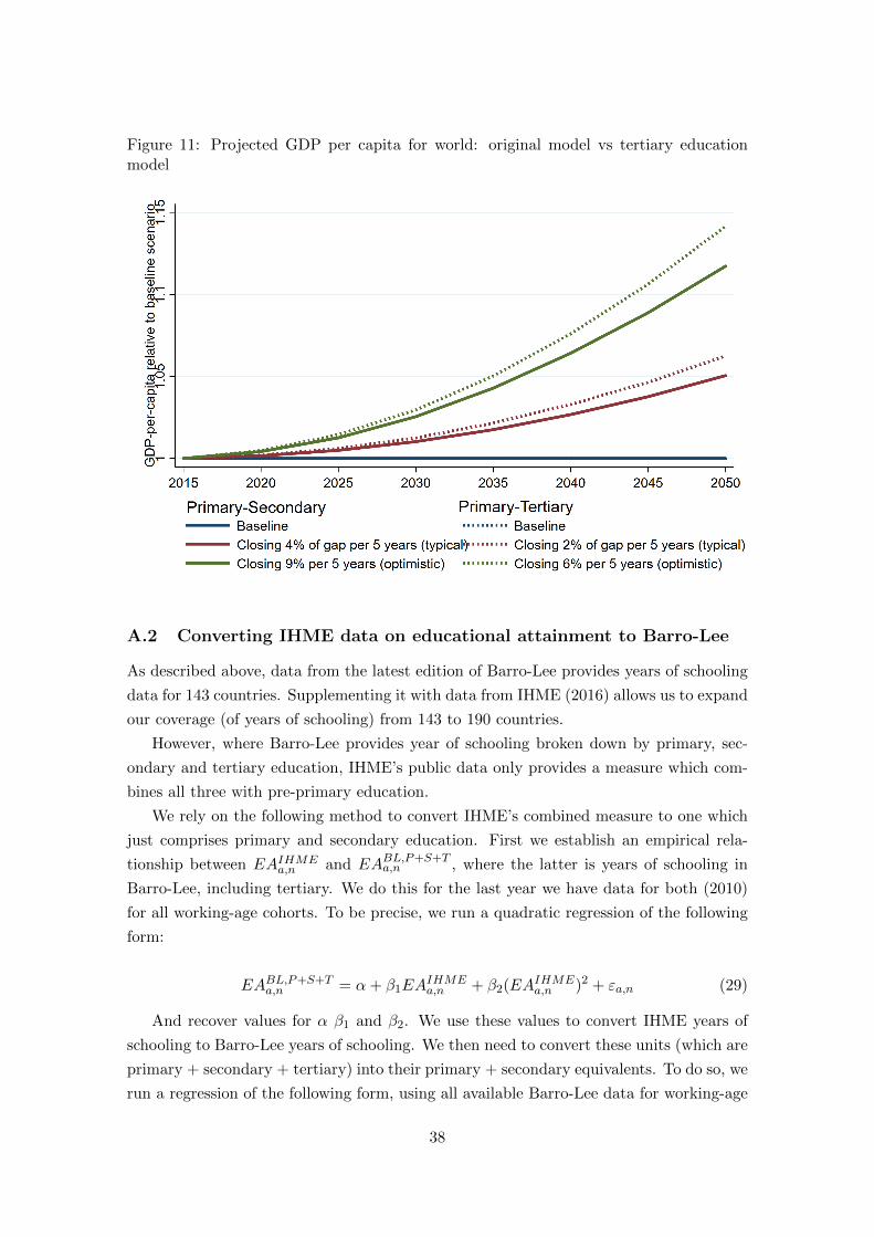
Figure 11: Projected GDP per capita for world: original model vs tertiary educationmodel

A.2 Converting IHME data on educational attainment to Barro-Lee

As described above, data from the latest edition of Barro-Lee provides years of schooling

data for 143 countries. Supplementing it with data from IHME (2016) allows us to expand

our coverage (of years of schooling) from 143 to 190 countries.

However, where Barro-Lee provides year of schooling broken down by primary, sec-

ondary and tertiary education, IHME’s public data only provides a measure which com-

bines all three with pre-primary education.

We rely on the following method to convert IHME’s combined measure to one which

just comprises primary and secondary education. First we establish an empirical rela-

tionship between EAIHMEa,n and EABL,P+S+T

a,n , where the latter is years of schooling in

Barro-Lee, including tertiary. We do this for the last year we have data for both (2010)

for all working-age cohorts. To be precise, we run a quadratic regression of the following

form:

EABL,P+S+Ta,n = α+ β1EA

IHMEa,n + β2(EA

IHMEa,n )2 + εa,n (29)

And recover values for α β1 and β2. We use these values to convert IHME years of

schooling to Barro-Lee years of schooling. We then need to convert these units (which are

primary + secondary + tertiary) into their primary + secondary equivalents. To do so, we

run a regression of the following form, using all available Barro-Lee data for working-age

38

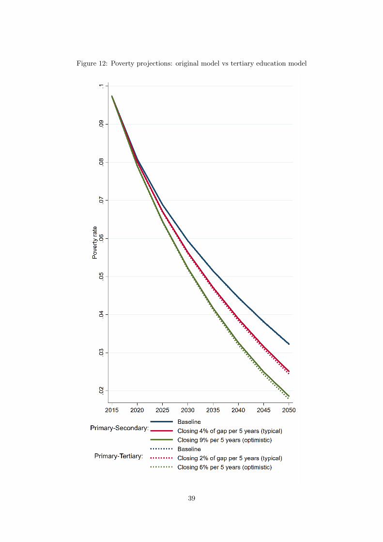
Figure 12: Poverty projections: original model vs tertiary education model

39

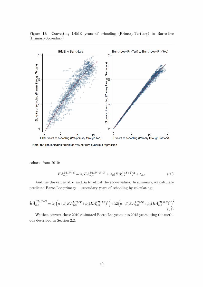
Figure 13: Converting IHME years of schooling (Primary-Tertiary) to Barro-Lee(Primary-Secondary)

cohorts from 2010:

EABL,P+Sa,n = λ1EA

BL,P+S+Ta,n + λ2(EA

P+S+Ta,n )2 + εa,n (30)

And use the values of λ1 and λ2 to adjust the above values. In summary, we calculate

predicted Barro-Lee primary + secondary years of schooling by calculating:

EABL,P+S

a,n = λ1

(α+β1EA

IHMEa,n +β2(EA

IHMEa,n )2

)+λ2

(α+β1EA

IHMEa,n +β2(EA

IHMEa,n )2

)2(31)

We then convert these 2010 estimated Barro-Lee years into 2015 years using the meth-

ods described in Section 2.2.

40