1

The Effect of Early Childhood Malnutrition on Child Labor and

Schooling: Theory and Evidence*

Solomon Tesfay Tesfu**

Center for Policy Research

Maxwell School of Syracuse University

November 2010

Abstract

This paper examines how physical stature of a child measured in terms of age

standardized height influences his/her selection for family labor activities vs. schooling in

rural Ethiopia using malnutrition caused by exposure to significant weather shocks in

early childhood as sources of identification for the child‘s physical stature. I estimate

parametric and semi-nonparametric bivariate models for child labor and schooling. I find

no evidence that better physical stature of the child leads to his/her positive selection for

fulltime child labor activities. On the other hand I found reasonably strong and consistent

evidence that physically more robust children are more likely to combine child labor and

schooling than physically weaker children. The results are consistent across two different

cohorts of children and two different identification strategies. The findings indicate that,

although better early childhood nutrition leads to higher chances of attending school, it

may also put the child at additional pressure to participate in family labor activities which

may be reflected in poor performance in schooling. Therefore, policies that try to

promote schooling through nutrition support programs could be more successful if they

are accompanied by programs that could mitigate the family‘s needs for child labor like

income support schemes.

JEL Classification: I0

KEYWORDS: Height-for-age; child schooling; child labor; weather Shocks; bivariate model;

semi-nonparametric

1. Introduction

Unlike the developed economies where short-term fluctuations in household income and

living standards are largely associated with the conditions in the labor market and business

* I thank Shiferaw Gurmu, Barry Hirsch, Erdal Tekin, Jose Canals-Cerda, Paula Stephan, Ragan Petrie, Inas

Rashad, Petra Todd and Umut Ozek for invaluable suggestions and comments that have helped to considerably

improve this paper. All the remaining errors are mine. **

Corresponding address: Center for Policy Research, Maxwell School of Syracuse University, 426 Eggers Hall, Syracuse, NY 13244-1020; Phone: (703) 298-7481; Fax: (315) 443-1081; E-mail: sttesfu@maxwell.syr.edu

2

cycles, temporary changes in livelihoods of rural communities in the least developed economies

are often caused by changes in weather conditions. In such communities, large and unexpected

changes in weather conditions can sometimes have a devastating impact on income,

consumption, assets, health and survival of households and their members. Drought, flooding,

hailstorms, cyclonic storms, and frost are some of the weather related shocks that frequently

affect the livelihoods of rural communities in developing countries. A large number of studies

have investigated the impacts of such shocks and how households try to cope with their effects.

The overall picture that emerges from the multitude of empirical studies is that the ultimate

impact of a shock on the well-being of a household and its members depends on a number of

household and community-specific characteristics such as liquidity constraints, wealth status,

and the nature and capabilities of social support networks to which households belong (see

Townsend 1995; Murdoch 1999; Carter and Maluccio 2003).

One important indicator of the capability of households to absorb the effects of a shock is

whether the nutritional status of its members, as reflected in anthropometric health measures,

substantially deteriorates as a result of the shock. While some evidence shows that adults may

lose some body mass (Dercon and Krishnan 2000) as a consequence of shocks, the majority of

empirical studies show that it is children in their first 3 years of life at the time of the shock who

are particularly vulnerable. This is not surprising given that this is a period when children are

growing fast and have high nutritional requirements per unit of body mass (Martorell et al. 1995;

Martorell 1999; Hoddinott and Kinsey 2001). Another reason for the high nutrition requirements

for young children is their vulnerability to diseases because of immature immune systems and

the inability to make their needs known.

Some studies have examined the extent to which exposure to a shock at this early age

affects the physical stature of the person later in life. While some evidence from the United

States shows that reversal of the effects of early malnutrition is possible if there are dramatic

favorable changes in the environment for the child at the appropriate time (Golden 1994), studies

from developing countries (e.g., Alderman, Hoddinott and Kinsey 2006) show that victims of

severe shocks in early childhood often sustain long-lasting deficiencies in their physical stature

and possibly cognitive ability (Dasgupta 1997). Other studies have looked at how the effects of

malnutrition on the child‘s health stature may be related to the child‘s schooling outcomes (e.g.,

Behrman and Lavy 1994; Glewwe and Jacoby 1995; Glewwe and King 2001; Glewwe, Jacoby

and King 2001; Alderman et al. 2001) and largely find that preschool malnutrition has negative

effect on a child‘s school enrollment and academic performance. One of the often stated reasons

for this relationship between schooling and early childhood malnutrition (stunting) is that

families are unwilling or hesitant to send a physically unfit child to school, in addition to the

effect of childhood malnutrition on cognitive development that may be reflected in his/her poor

performance or progress at school.

The largely uneducated parents in developing countries, however, may be less likely to

recognize the potential correlation between physical fitness and cognitive abilities than they are

to recognize the importance of a child‘s physical strength for family labor. Consequently, parents

may end up sending the physically weaker children to school and keep the robust ones for family

labor or demand more of their after school time for family labor activities. As a result, studies

that ignore the importance of physical stature for child labor (where child labor also matters)

may end up with results that understate the effect of malnutrition on enrollment but overstate

3

malnutrition‘s effect on school performance. This is so because it is largely the weaker children

with potentially lower cognitive abilities (since malnutrition also hampers child‘s cognitive

development, Dasgupta 1997) who would be sent to school. Equity considerations may reinforce

the possibility of sending a physically weaker child to school over a stronger sibling if parents

feel that the weaker child will have a hard time succeeding in the labor market if he/she doesn‘t

acquire additional skills. Therefore, understanding the role of physical stature of a child in the

family‘s choices between schooling and child labor is not only an important research question in

itself but also may help to refine and better understand the observed relationships between

childhood malnutrition shocks and academic performance. One issue in using child‘s physical

stature as a covariate in the schooling and child labor equations, however, is that it could be

endogenous in both equations because parents might have been making child nutrition decisions

in anticipation of specific role for the child. Therefore, an exogenous source of variation in

nutritional status that is beyond the control of the parents is needed to identify its effect on

schooling and child labor.

In this paper I use two sources of exogenous variation in availability of food (and

possibly other amenities) during the critical ages of the child to jointly analyze the effect of early

childhood malnutrition on schooling and child labor.1 First I exploit the natural experiment

generated by a massive drought in Ethiopia in 1984 that resulted in a devastating famine that

killed about a million people in the country (Jansen, Harris and Penrose 1987). Second, I use the

considerable annual fluctuations in rainfall in some localities in the country to identify local

weather shocks and the subsequent food deficits in the areas and use these as exogenous sources

of malnutrition. In Ethiopia about 85% of the people live on a subsistence agriculture that is

almost fully dependent on rainfall conditions. As a result rainfall failures often have big effects

on the welfare of households and their members. While grown-ups and older children might also

suffer under famines and may sustain some long-term deficiencies in their health and fitness,

there is a general consensus in the literature that it is the children at the early years of their life

that sustain the biggest long-term damage in their stature and possibly cognitive abilities

(Dasgupta 1997). The key purpose of this paper is, therefore, to examine how potential

deficiencies in physical stature sustained from early childhood malnutrition are reflected in the

child‘s participation in schooling and family labor.

The rest of the paper is organized as follows. A simple theoretical model presented in the

section 2 demonstrates the effect of physical stature on child activity choice. Section 3 presents

empirical models, identification strategies as well estimation methodology. The data used in

empirical analysis are described and summary statistics are presented in section 4. Section 5

presents empirical results while section 6 concludes.

2. Theory

The basic research question in this paper can be described in a simple household utility

maximization model for a family with one child and unified preferences as in Ravallion and

Woodon (2000) and Bacolod and Ranjan (2008) among others. For convenience the child‘s life

1 Porter (2007) analyzed the effect of the 1984 drought shock on the long-term indicators of child nutrition health

using data from the first round of the Survey that I’m using. But the first stages of my empirical models in this paper expand her analysis by estimating the effects of localized rainfall shocks on the long-term nutritional status using data from a different cohort of children.

4

is classified into three periods: preschool age, school age and post-school age. In the preschool

period, the parents invest in the health of the child in the form of nutrition, health care and other

treatments. The health of the child in this period could also be influenced by factors beyond the

control of the family like weather shocks and availability of health care services. In the second

period parents decide whether to send the child to school or to child labor. In the third period,

the child works and earns his/her own income, while parents retire and consume the return on the

assets they saved during the earlier periods and possible transfers from their children. The focus

here is on the decision problem that parents face in the second period given the outcome of their

decisions in the first period.

Assuming that parents are altruistic towards their children and the utility parents derive

from own consumption is linearly separable from that they derive from the child‘s utility as in

Barro and Becker (1986), Cigno and Rosati (2005) and Dillon (2008), among others, the

parents‘ utility may be stated as

t

ccp

tt yccUcuU ),,(*)( 321 t=1, 2, 3 (1)

where, p

tc is parents‘ consumption in period t, U* is child‘s maximized utility, cc1 is child‘s

consumption in period 1 including healthcare, cc2 is child‘s consumption in period 2 including

healthcare but excluding school expenses, y3 is child‘s income in the post-school period and β is

a measure of parental altruism towards the child where 0<β≤1. Both ut(.) and U*(.) are assumed

to be quasi-concave and strictly increasing in all of their arguments. In period 2, pc1 and

cc1 are

no longer part of the decision problem of the parents. However, cc1 determines the child‘s pre-

school stock of human capital in the form of physical stature and cognitive ability, given the

child‘s genetic and natural endowments. And according to the literature on nutrition physical

stature at the preschool age (that is also correlated with cognitive ability) is a strong predictor of

the later physical stature of the child as previously discussed. Let h1 denote this preschool

physical stature of the child measured in terms of height-for-age. Assuming that the trajectory for

the physical human capital of the child is completely set in the preschool age and building on

Glewwe (2002), the human capital production function of the child in period 2 may be stated as

),(),( 1 QTshh s

c (2)

where, γ(.) is the ‗learning efficiency‘ of the child that depends on the unobserved factors (µ)

that include genetically inherited ability, child‘s motivation, etc. as well as the child‘s physical

fitness accumulated during the preschool period (h1). On the other hand, s(.) is the schooling

production function that depends on the amount of child‘s time spent in schooling and studying, s

cT , and a vector of other educational inputs and school characteristics, Q. In period 2, γ(.) is

assumed to be predetermined while the interaction between γ(.) and s(.) produces new human

capital. For simplicity accumulation of long-term human capital is assumed to be independent of

fluctuations in consumption after the preschool period. That is why cc2 is not included as an

argument in human capital production function for period 2.

The human capital the child accumulates through period 2 along with the net parental

transfers determines his/her income in the post school period, y3:

5

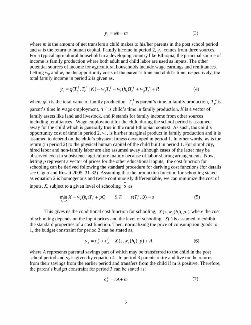
mhy 3 (3)

where m is the amount of net transfers a child makes to his/her parents in the post school period

and ω is the return to human capital. Family income in period 2, y2, comes from three sources.

For a typical agricultural household in a developing country like Ethiopia, the principal source of

income is family production where both adult and child labor are used as inputs. The other

potential sources of income for agricultural households include wage earnings and remittances.

Letting wp and wc be the opportunity costs of the parent‘s time and child‘s time, respectively, the

total family income in period 2 is given as,

RTwThwTwKTTqy w

pp

f

cc

f

pp

f

c

f

p )()|,( 12 (4)

where q(.) is the total value of family production, f

pT is parent‘s time in family production, w

pT is

parent‘s time in wage employment, f

cT is child‘s time in family production, K is a vector of

family assets like land and livestock, and R stands for family income from other sources

including remittances . Wage employment for the child during the school period is assumed

away for the child which is generally true in the rural Ethiopian context. As such, the child‘s

opportunity cost of time in period 2, wc, is his/her marginal product in family production and it is

assumed to depend on the child‘s physical fitness developed in period 1. In other words, wc is the

return (in period 2) to the physical human capital of the child built in period 1. For simplicity,

hired labor and non-family labor are also assumed away although cases of the latter may be

observed even in subsistence agriculture mainly because of labor-sharing arrangements. Now,

letting p represent a vector of prices for the other educational inputs, the cost function for

schooling can be derived following the standard procedure for deriving cost functions (for details

see Cigno and Rosati 2005, 31-32). Assuming that the production function for schooling stated

as equation 2 is homogenous and twice continuously differentiable, we can minimize the cost of

inputs, X, subject to a given level of schooling s as

pQThwX s

ccQT s

c

)(min 1,

S.T. sQTs s

c ),( (5)

This gives us the conditional cost function for schooling, )),(,( 1 phwsX c where the cost

of schooling depends on the input prices and the level of schooling. X(.) is assumed to exhibit

the standard properties of a cost function. Then, normalizing the price of consumption goods to

1, the budget constraint for period 2 can be stated as,

AphwsXccy c

cp )),(,( 1222 (6)

where A represents parental savings part of which may be transferred to the child in the post

school period and y2 is given by equation 4. In period 3 parents retire and live on the returns

from their savings from the earlier period and transfers from the child if m is positive. Therefore,

the parent‘s budget constraint for period 3 can be stated as:

mrAc p 3 (7)

6

where r is return on parental assets. The net parental transfers could be positive if child-to-parent

transfers exceed parent-to-child transfers. Substituting 7 and 3 for pc3and 3y in equation 1

respectively, and then substituting equation 2 for h the family‘s utility function in period 2 can be

rewritten as,

)),((.),(*)()( 2322 mQTscUmrAucuU s

c

cp (8)

Note that u1(.) is no longer relevant in period 2 and hence ignored. Assuming that the

non-negativity constraints for consumption and parental savings are non-binding and also

assuming that the time constraint for both the parents and the child is non-binding so that the

Lagrangian multipliers on all these constrains are 0, we can maximize2 8 subject to 6 to obtain

the conditions that determine parental decisions on consumption, savings and time use for

themselves and for the child. The Lagrangian function for the maximization problem is,

])),(,(

)()|,([

)),((.),(*)()(max

122

21

2322,,,,,,, 22

AphwsXccR

TwThwTwKTTq

mQTscUmrAucuL

cp

w

p

ps

cc

f

pp

f

c

f

p

s

c

cp

QTTTTAcc fp

wp

fc

sc

cp

(9)

The first order conditions that are relevant for the purpose at hand are,

:2

pc

0(.)

2

2

pc

u (10)

:2

pc

0(.) 3

3

3

A

c

c

u p

p

pc

ur

3

3 (.) (11)

:2

cc

0(.)*

2

cc

U (12)

:s

cT

0(.)*

(.) 3

3

s

c

s

c T

s

s

X

T

s

s

h

h

y

y

U

s

X

s

h

y

U

3

(.)*(.)

(13)

:f

cT

0)]([ 1

hw

T

qcf

c

)(),|( 1hwTKTMP c

f

p

f

c

f

Tc

(14)

Condition 14 states that the marginal product of the child‘s time in family production in

period 2 equals the opportunity cost of the child‘s time that itself is assumed to depend on the

child‘s physical fitness accumulated during the preschool period. In 13 sX is the marginal

2 In writing the maximization problem without the expectations operator, we are assuming that parents face no

uncertainty about the values of the third period variables like the return to human capital.

7

cost of schooling that is henceforth denoted by MCs and sh is the marginal productivity of

schooling in the production of overall human capital henceforth denoted by h

sMP . The marginal

cost of schooling depends on the level of schooling, the opportunity cost of the child‘s time and

price of other educational inputs. Dividing 10 by 11 we obtain,

r

c

mrAu

c

cu

MRS

p

p

p

p

cc

3

3

2

22

)(

)(

2,3 (15)

The middle term in 16 is the marginal rate of inter-temporal substitution between current

consumption and future consumption for the parents (p

ccMRS23 , ). The equation states that parents

save for their future consumption until the marginal utility of the current consumption relative to

their future consumption is equated to the return on savings (the interest rate). The analogous

condition for the child is obtained by dividing 12 by 13,

)),(,(

(.)

)),((.),(*

)),((.),(*

1

3

2

2

2

2,3 phwsMC

MP

ymQTscU

c

mQTscU

MRScs

h

s

s

c

c

c

s

c

c

c

cy

(16)

The middle term in 16 is the marginal rate of inter-temporal substitution between current

consumption and future income for the child (c

cyMRS23 , ). The term in the parenthesis on the right

hand side of this equation may be interpreted as the marginal return to investment in schooling in

terms of building the overall human capital of the child. The entire term on the right hand side

then represents the marginal return to human capital built through schooling. Note that the

effectiveness of investment in schooling in building the overall human capital (knowledge and

capability) of the child depends on the learning efficiency of the child and marginal productivity

of schooling in the production of human capital. While some of the learning efficiency could be

genetic and may be acquired through inheritance, part of it is built through investment in

nutrition and healthcare during the preschool period. However, it is assumed that parents treat

these as sunk costs when they make decisions about consumption and time use in period 2.

Assuming that parents try to allocate the family‘s resources so as to maximize the life

time utility for themselves and the child and given that total utility is strictly increasing in both

the parents‘ and the child‘s consumption, they will allocate the child‘s time between s

cT and f

cT

by comparing the future marginal return to investment in human capital (given by the right hand

side of 16) to the return that the child‘s contribution to the current income could bring in if it

were to be saved for future consumption (r). If ]/(.)[ s

h

s MCMPr , then parents are likely to

allocate more of the child‘s time to generating current income through child labor and less to

schooling since marginal return to asset savings is greater than the marginal return to human

capital. On the other hand, if ]/(.)[ s

h

s MCMPr , then parents are likely to allocate more of

the child‘s time to schooling and less to family work since marginal return to human capital in

the future is greater than the marginal return to savings. Therefore, the optimal allocation of the

child‘s time between schooling and current income generating activities is given by,

8

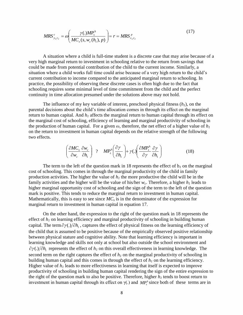
(17)

A situation where a child is full-time student is a discrete case that may arise because of a

very high marginal return to investment in schooling relative to the return from savings that

could be made from potential contribution of the child to the current income. Similarly, a

situation where a child works full time could arise because of a very high return to the child‘s

current contribution to income compared to the anticipated marginal return to schooling. In

practice, the possibility of observing these discrete cases is often high due to the fact that

schooling requires some minimal level of time commitment from the child and the perfect

continuity in time allocation presumed under the solutions above may not hold.

The influence of my key variable of interest, preschool physical fitness (h1), on the

parental decisions about the child‘s time allocation comes in through its effect on the marginal

return to human capital. And h1 affects the marginal return to human capital through its effect on

the marginal cost of schooling, efficiency of learning and marginal productivity of schooling in

the production of human capital. For a given ω, therefore, the net effect of a higher value of h1

on the return to investment in human capital depends on the relative strength of the following

two effects.

1h

w

w

MC c

c

s ?

11

(.)h

MP

hMP

h

sh

s

(18)

The term to the left of the question mark in 18 represents the effect of h1 on the marginal

cost of schooling. This comes in through the marginal productivity of the child in family

production activities. The higher the value of h1 the more productive the child will be in the

family activities and the higher will be the value of his/her wc. Therefore, a higher h1 leads to

higher marginal opportunity cost of schooling and the sign of the term to the left of the question

mark is positive. This tends to reduce the marginal return to investment in human capital.

Mathematically, this is easy to see since MCs is in the denominator of the expression for

marginal return to investment in human capital in equation 17.

On the other hand, the expression to the right of the question mark in 18 represents the

effect of h1 on learning efficiency and marginal productivity of schooling in building human

capital. The term 1(.) h , captures the effect of physical fitness on the learning efficiency of

the child that is assumed to be positive because of the empirically observed positive relationship

between physical stature and cognitive ability. Note that learning efficiency is important in

learning knowledge and skills not only at school but also outside the school environment and

1(.) h represents the effect of h1 on this overall effectiveness in learning knowledge. The

second term on the right captures the effect of h1 on the marginal productivity of schooling in

building human capital and this comes in through the effect of h1 on the learning efficiency.

Higher value of h1 leads to more effectiveness in learning that itself is expected to improve

productivity of schooling in building human capital rendering the sign of the entire expression to

the right of the question mark to also be positive. Therefore, higher h1 tends to boost return to

investment in human capital through its effect on γ(.) and h

sMP since both of these terms are in

p

cc

cs

h

sc

cy MRSrphwsMC

MPMRS

2,32,3 )),(,(

(.)

1

9

the numerator of the expression for the return to investment in human capital stated under

equation 17.

The net effect of h1 on the marginal return to investment in human capital will be

negative if its effect on MCs is stronger than its combined effect on γ(.) and h

sMP . For given

values of r, ω and parental preferences, therefore, parents will have an incentive to keep a

physically stronger child out of school so as to engage in the child labor activities. This means,

parents believe that the marginal productivity of such a child in the current family activities is

higher than whatever future gains (net of the cost of schooling) in earnings the child could

achieve through schooling. On the other hand, if the combined effect of h1 on the overall

efficiency of learning and the marginal productivity of schooling is stronger than its effect on

MCs, parents will have an incentive to send the child to school. Whether parents allow the child

to be a full time student by letting him/her to focus on studying even after coming back from

attending school or ask him/her to work after school can be established following similar

reasoning. This is so because studying after school is part of the human capital building process

whose opportunity cost could be measured by the marginal productivity of the child in family

activities just like attending school. Therefore, the effect of physical stature of the child on child

labor and schooling is theoretically ambiguous as opposed to the prevailing wisdom that it

enhances the chances of attending school.

To empirically test the implications of this theoretical model, we need to derive the

parental demand functions for own and child‘s consumption as well as time use. When specific

structural forms are assumed for the utility function, specific forms for the demand functions can

be derived by simultaneously solving the relevant first order conditions stated above and the

budget constraint stated under 6. For a general form of the utility function assumed here,

however, the demand functions will take the following general forms.

),,,,,,,( 1

* rmwRphTT p

s

C

s

c (19)

),,,,,,,( 1

* rmwRphTT p

f

c

f

c (20)

The demand functions for other choice variables*

2

cc , *

2

pc , *f

pT , *w

pT , A* and Q* take

similar general forms. It is important to note that these demand functions are interdependent

because of the simultaneous nature of parental decisions. This is particularly magnified in the

case of time use decisions because of the fixed time constraint. For a child constrained with only

24 hours a day, more time for family labor means less time for attending school and studying

then after. Therefore, joint estimates of the demand functions will generally provide more

accurate estimates of the effects of the covariates on each of the parental choices than the

estimates from independent equations for each demand function. This is so because some of the

factors that influence parental decisions may not be observable and hence cannot be included as

regressors in each equation. As a result the errors that include these unobservables will be

correlated across equations and joint estimation techniques that exploit these correlations will

lead to more accurate estimates.

To specify such joint empirical models for parental demand for child labor and schooling

we first define the indirect utility function for the parents, ),,,,,,,( 1 rmwRphv p, by

10

successively substituting the relevant demand functions into 2, 3, and 7 and the resulting

functions into 8 along with *

2

cc and *

2

pc . The indirect utility function is thus defined in terms of

observables. From the researcher‘s perspective, however, there are unobservable elements that

may influence parents‘ decisions and restating the utility function by adding these random

components to the indirect utility provides the basis for the empirical model specified in the next

section.

3. Econometric Models and Estimation Methodology

The main purpose of this paper is to analyze the effect of physical stature of a child in the

form of height-for-age z-scores on his/her participation in child labor and schooling. The

empirical model for the analysis has to allow for the potential correlation between the error terms

of the schooling and child labor equations that arises because of the joint nature of the two

decisions. Such a model can be specified by adding unobserved random components to the

indirect utility parents derive from child schooling and work as,

isisis vu (.)*

(21)

iwiwiw vu (.)*

(22)

where vis(.) and viw(.) denote maximized utilities from schooling and child work from the

theoretical model, εis and εiw denote the corresponding random components, *

isu and *

iwu represent

additive random utility (Cameron and Trivedi 2005) parents derive from child i‘s participation in

schooling and family work , respectively. Assuming that vis(.) and viw(.) are linear in their

arguments, 21 and 22 can be restated as,

issisis xu '*

(23)

iwwiwiw xu '*

(24)

where '

ijx represents a vector of covariates including my key variable of interest, physical stature

of the child (h1). The latent variables, *

isu and *

iwu , are unobserved but let‘s assume that parents

send a child to school or work only when the overall utility from doing so is positive. Then we

can define the following dichotomous variables for child‘s participation in schooling and family

work, respectively.

00

01

*

*

is

is

iuif

uifs (25)

00

01

*

*

iw

iw

iuif

uifw (26)

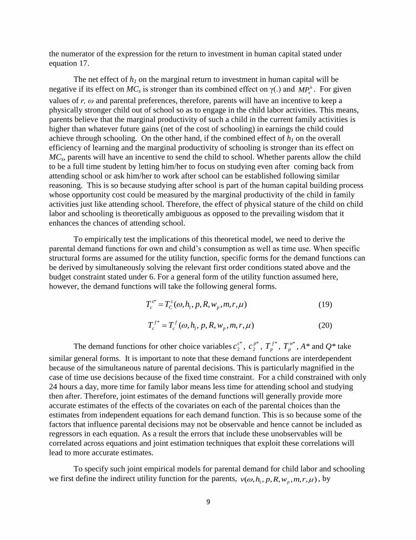
The four possible choices parents can make regarding child i‘s time use are: si=0, wi=0;

si=0, wi=1; si=1, wi=0; and si=1, wi=1. Assuming that εiw and εis are distributed jointly normal

11

with means zero, variances one, and correlation , the probabilities of observing each of these

joint outcomes can be specified as bivariate normal. For example, the probability of observing

si=1, wi=1 can be stated as,

27),,(

),,(

],[

]0,0[

]1,1[

''

''

**

"'

wiwsis

x

wsws

x

wiwiwsisis

iwis

iiik

xx

dzdzzz

xxp

uup

wspp

wiwsis

where (.) and Ф(.) are the standardized bivariate normal density and the cumulative density

function for (zs, zw), respectively. We can state similar bivariate cumulative density and density

functions for the other three possible outcomes. Following Green (2007), these can be

generalized as,

28),,(

],[

'' iwiswiwiwsisis

iiik

xx

kwjspp

where the indicator function δis=1 if si=1 and δis=-1 if si=0. Similarly, δiw=1 if wi=1 and δiw=-1

if wi=0. Then the log-likelihood function for the bivariate probit model can be stated as,

i

iwiswiwiwsisis xxL ),,(lnln '' (29)

The model under 29 is estimated using maximum likelihood procedure. I also estimate a

semi-nonparametric bivariate model for child schooling and labor using the procedure developed

in Gallant and Nychka (1987). In their approach, as slightly modified by De Luca (2008), the

unknown joint density of the errors is approximated by the Hermite series of the form,

)()(),(1

),( 2

wswsr

N

wsh

(30)

where, ϕ(.) is the standardized Gaussian density, j

w

i

sij

r

j

r

i

wsr

21

00

),( is a polynomial in

εs and εw of order r=(r1,r2) and, wswswsrN dd )()(),( 2

is a normalization

factor that ensures h(.) integrates to 1. Equation 30 approximates the joint density of the errors

as the product of a squared polynomial and a standardized bivariate normal density where the

latter is assumed just for convenience. Gallant and Nychka (1987) demonstrate that 30

approximates densities with arbitrary skewness and kurtosis except those that are violently

oscillatory. In implementation, the vector of parameters ),...,,(210100 rr is normalized by

setting 100 since the polynomial expansion in 30 is invariant to multiplication of the

12

parameter vector by a scalar. The specification of the pseudo–log-likelihood function and the

detailed procedures for implementation of the model are explained in De Luca (2008). This

approach not only relaxes the parametric assumption of the bivariate probit model in estimating

the coefficients but also allows detailed examination of the characteristics of the error densities

for different values of r1 and r2.

In addition to the child‘s height-for-age z scores as a measure of the child‘s physical

fitness, the vector of covariates in all the models includes child‘s age and gender, number of

siblings, livestock and land area owned as measures of the household‘s wealth status, parents‘

age and education, as well as distance to a primary school as a proxy for cost of schooling. The

indicators for household wealth could be thought of as proxies for household income, discussed

in the theoretical model. Information on household income gathered through surveys in the rural

areas of developing countries is often unreliable and wealth indicators could be better measures

of household well-being. Controlling for wealth indicators is important because the need for

child labor and the ability of the families to send their children to school could vary with wealth

status. Variation across households and changes over time in wealth indicators could also be

correlated with nutritional status of children; thus failing to control for wealth indicators could

bias my estimates. The theoretical model described above also implies that the wage rate for

child labor is a relevant variable that should be accounted for in the empirical model since the

wage paid to a child could be correlated with physical stature. However, child labor in rural

Ethiopia almost entirely consists of unpaid family labor, so information on formal wage rates for

children is unavailable. The child‘s opportunity cost of time is essentially his/her marginal

product in the family production activity and to the extent that the marginal productivity depends

on having other assets to work with, children in the families with more land and livestock could

have higher opportunity cost of time than children with less assets. Therefore, inclusion of land

and livestock ownership as covariates may partly control for the opportunity cost of the child‘s

time.

The vectors of coefficients from the bivariate probit models are used to calculate the

marginal effects of the covariates on the probability of observing each of the joint outcomes:

p(si=0, wi=0), p(si=0, wi=1), p(si=1, wi=0), and p(si=1, wi=1). For the purpose of comparison

with other studies that estimated an independent equation just for schooling, I also estimate the

standard probit models for the child‘s school attendance and participation in family work.

Therefore, the marginal effects of the covariates on p(si=1) and p(wi=1) are computed using both

the joint models as well as independent probit models. As briefly described in the previous

section, the marginal effect of my key variable of interest, child‘s physical stature on child

schooling and child labor is theoretically ambiguous. The existing literature generally argues

that better physical fitness enhances the chances that a child attends schooling implying that its

effect on p(si=1) will be strongly positive. The effects of physical fitness on the joint outcomes

have not been examined by the existing studies. Therefore, the estimates here help us to answer

an important question of whether child‘s physical fitness enhances the child‘s chances of being a

full time student, p(si=1, wi=0), or part-time student, p(si=1, wi=1), or even full-time worker,

p(si=0, wi=1).

One important issue that needs to be addressed in estimating these models is the potential

endogeneity of the child‘s physical stature in both schooling and child labor equations.

Endogeneity could arise because parents may be providing preferential treatment in terms of

13

nutrition to some children (particularly when resources are limited) in anticipation of specific

role for each child depending on their perceptions regarding the importance of physical fitness

for each of the child‘s anticipated roles. For example, parents may feed the oldest child very well

so that he/she quickly grows up and helps them in fulfilling the family labor needs. If this is the

case it may be the anticipated role for the child (schooling or labor) that is determining his

physical stature rather than the other way round and the estimates may not represent a causal

effect. Therefore, an exogenous source of variation in nutrition status that is beyond the control

of the parents is needed to identify its effects on schooling and child labor. Exposure to a famine

caused by a massive drought and localized rainfall shocks are used as identifying instruments as

discussed in the next section.

Another critical issue is how to implement instrumental variables estimation in the

context of these heavily nonlinear models for non-binary outcomes. There are at least three

approaches that have been used to address this issue in various contexts. One possibility is to

jointly estimate the first stage equation for the endogenous variable and the second-stage

equation for the outcome variable of interest, for example, using the full information maximum

likelihood approach to obtain asymptotically efficient estimators as initially proposed by

Hausman (1975) . However, the application of this method generally depends on some arbitrary

assumptions about the joint distribution of the errors in the two equations the validity of which

cannot be readily verified.

The other commonly applied method is what may be called ‗two-stage predictor

substitution‘ (2SPS) where the endogenous regressor in the second-stage equation is replaced by

its predicted value from a separately run auxiliary regression correcting the standard errors for

the resulting measurement error bias (for some of the recent applications of this method see Lu

and McGuire 2002; Meer and Rosen 2004; Savage and Wright 2003; Gramm 2003). Unlike the

linear models where the two-stage predictor substitution leads to consistent estimates, however,

the consistency of such estimates in the non-linear context has not been well established. In fact

Terza, Basu and Rathouz (2008) show that such a method generally leads to inconsistent

estimates in the non-linear models. On the other hand, they demonstrate that an alternative

method that requires inclusion of the residual from the first-stage auxiliary regression in the

second-stage equation provides consistent estimates. The two-stage residual inclusion (2SRI)

method has been recently used by a number of empirical studies (see Stuart, Doshi, and Terza

2009; Shea et al. 2007; Gibson et al. 2006; Shin and Moon 2007; DeSimone 2002; Baser et al.

2004) but its theoretical properties in such applications have not been formally examined until

the latest work by Terza, Basu and Rathouz (2008).

According to Terza, Basu and Rathouz (2008) the 2SRI method provides consistent

estimates because the unobserved factors that led to endogeneity of the regressor can be

controlled for by the residuals from the first stage auxiliary regression as long as we can find

valid identifying instruments. This method provides not only consistent estimates but

asymptotically correct standard errors. They test their theoretical results about the consistency of

the 2SRI and inconsistency of 2SPS estimates using simulated data with 5,000 and 20,000

observations. They find negligible biases in the 2SRI estimates and several times larger biases in

the 2SPS estimates for a duration model with multinomial endogenous treatments and ordered

logit model with count-valued endogenous treatments. They apply the two methods to actual

data as well and find that the 2SPS method substantially overestimates the effect of the

14

endogenous variable. Therefore, I use the 2SRI method to address the potential endogeneity of

the child‘s physical stature in the bivariate probit models for child labor and schooling where the

first stage is a linear model for the child‘s height-for-age z scores. The two-stage approach fits

the models here conceptually as well because parental decisions are formulated as sequential

where the early period focuses on building the physical fitness of the child through nutrition and

health services and the subsequent period largely focuses on allocating the child‘s time to

schooling or family labor or both.

3.1 Identification Strategy

The findings in the literature on nutrition indicate that there is strong relationship

between height-for-age in early childhood and height-for-age later in life (e.g., See Martorell et

al. 1995; Martorell 1999, 1997). In fact Martorell et al. conclude that ―regardless of the choice of

reference population, growth is markedly retarded only in early childhood; adolescence is not a

period when growth is significantly constrained‖ (p.1060S). This implies that factors that

significantly affect the child‘s nutritional status during early childhood are likely to be strongly

correlated with the child‘s cumulative nutrition outcome, say height-for-age, later in life.

Therefore, if one could find exogenous shocks that could substantially influence the child‘s

nutrition during early childhood, these shocks must be correlated with the child‘s cumulative

nutrition outcomes later in life and hence can be used to identify the effect of the latter on other

outcomes for the child like schooling and child labor. Using contemporaneous shocks in such

contexts may not be appropriate because they may influence the schooling and child labor

outcomes directly, for example by putting the household under resource pressure. On the other

hand shocks that happened well in the past are less likely to be directly correlated with current

child labor and schooling outcomes except through their long-lasting effect on the child‘s

physical and cognitive abilities.

The fact that the livelihoods of the rural communities in Ethiopia are highly dependent on

rainfall conditions provides an opportunity to use rainfall related shocks to identify the effects of

early childhood malnutrition on child outcomes later in life. Two approaches are followed in

using the rainfall related shocks for this purpose. First, an attempt is made to exploit a famine

caused by a massive drought in 1984 where the average rainfall nationwide was 22% below the

long-term average, making it the worst drought since rainfall data started to be systematically

recorded in 1961 (Webb, von Joachim and Yohannes 1992). While household level data on

experience during the famine are largely unavailable, in 1995 a sample of 1477 households from

15 different sites in the country were asked to recall the three biggest droughts over the previous

20 years in which they lost a substantial amount of their harvest and/or livestock. Nearly half the

households reported to have lost substantial crop harvest and/or livestock because of the drought

in 1984/85 agricultural seasons. The ages of the children in these sample households could be

traced back to the time of the drought to identify the group of children who were particularly

vulnerable (1 to 3 years old according to the literature on nutrition). These potentially affected

children would have been 10 to 12 years old in 1994.

The interactions between dummy variables that identify these children and a dummy

variable that identifies households who reported to have faced a substantial shock at the time are

used as the first set of identifying instruments for early childhood malnutrition. That is, the

identifying instruments are generated by interacting a dummy for the reported household level

shock with a dummy for being age 1, a dummy for being age 2 and a dummy for being age 3 in

15

1984. Children who were 4 to 6 years old at the time of the drought (13 to 15 years old in 1994)

are included as controls. These are children who must have been less vulnerable at the time of

the drought and must have not sustained substantial damage in their physical stature from the

shock.3 Because of the observed linearity in the relationship between height-for-age in early

childhood and later in life (Martorell et al. 1995), the age-shock interactions correlated with

height-for-age in the early childhood period should be correlated with height-for-age in 1994 and

the subsequent periods. To control for the genetic variation in height I also include the mother‘s

and father‘s height as additional covariates in the first stage regressions for child‘s height-for

age.4 This approach is implemented using data from the first round of the Ethiopian Rural

Household Survey (ERHS) conducted in 1994 and another round in 1995.

In the absence of detailed data on household experience at the time of the drought,

however, the famine shock may still be an imperfect way to accurately identify the degree of

malnutrition faced by children from different households. This is so because the capabilities of

the households to cope with crop and livestock loss might differ. Another issue with using the

famine shocks to identify the effects of malnutrition is that children who survived the famine and

are found alive in 1994 could be the stronger ones who could withstand the effects of the

drought, while weaker children might have already died, in which case the effect of the shock

could be understated.5 Another concern with this approach is that parents‘ age recalls may entail

some errors in a situation where formal records of child‘s birth date are not kept, as is largely

true in rural Ethiopia. This may be a more serious problem particularly when age recalling

involves longer time periods.

As a way of validating the results from the 1984-drought based identification strategy,

therefore, an alternative strategy based on localized rain-fall shocks is implemented using data

from a different cohort of children who were 1 to 6 years old at the time of the first round of the

survey in 1994. The fact that the birth dates for these children are relatively close to the survey

period is expected to make it easier for the parents to accurately recall the child‘s age and hence

minimize the potential age-recall error bias. The localized rainfall shocks are defined on the basis

of the deviations of the annual rainfall in the locality from its long-term mean.6 Both substantial

rain deficits and excessive rains are considered rainfall shocks since both can lead to crop failure.

Substantial rain deficit is represented by a dummy that takes a value of 1 if the rainfall shortfall

from the long-term mean is bigger than 1 standard deviation and excessive rainfall shock is

represented by a dummy taking a value of 1 if the excess of rain over the long-term mean

exceeds 1 standard deviation. Because of the erratic nature of rainfall in most localities in

Ethiopia, the long-term standard deviations of rainfall are quite large representing more than

15% of the mean annual rainfall on average. Therefore, rainfall deficits and excesses exceeding 1

standard deviation represent substantial shock that may lead to crop failures and significant

reductions in consumption in rural Ethiopia. For example, Dercon (2002) finds that a 10%

3 Children who were born at and after 1984 may not be an effective comparison group because they may also have

been the victims of the after-effects of the drought at their critical age. These children, therefore, are excluded from the sample. 4 Mother’s height was used for similar purpose by Glewwe and Jacoby (1995).

5 But the data on mortality history gathered during the 1995 round of the survey don’t show any unusually high

mortality in 1984 for the age group included in our sample. 6 A similar strategy was followed by Maccini and Yang (2009).

16

decrease in rainfall from the long-term mean decreases food consumption by up to 5% and

localized rainfall shortfalls of this magnitude or bigger are quite common in Ethiopia.

Therefore, the rainfall shocks faced by a child during the first 3 years of life are taken as

exogenous indicators of early childhood malnutrition and hence used as instruments for the

child‘s age-standardized heights in the child labor and schooling models. In this case height-for-

age measured towards the end of the preschool period is used since the anthropometric data were

gathered for all members of the sample households in 1994, 1995 and 1997. The genetic

variations in children‘s height are controlled for by mother‘s and father‘s heights in this approach

as well. Malnutrition induced by exogenous rainfall shocks is expected to explain what is left of

these natural differences in the heights of children. The schooling and child labor models for this

cohort of children are estimated using data from the latest two rounds of the survey conducted in

1999 and 2004. The age range for this cohort in 2004 is similar to the age range for the older

cohort in 1994. Therefore, results from the two identification strategies are expected to be at least

qualitatively comparable although rainfall shortfalls might be weaker instruments than the major

famine shock.

4. Data and Summary Statistics

The analysis in this paper is based on data from the various rounds of the Ethiopian rural

household survey (ERHS) conducted by the Economics Department of Addis Ababa University

in collaboration with the Center for the Study of African Economies at the University of Oxford,

the International Food Policy Research Institute (IFPRI) and the US Agency for International

Development (USAID). ERHS is a unique longitudinal data set in Ethiopia the first round of

which was conducted in 1994 (subsequently referred to as 1994a) and covered 1477 households

from 15 different sites across the country. Another round was conducted later in 1994

(henceforth referred to as 1994b) followed by one round each in 1995, 1997, 1999 and 2004. The

attrition rate was small between successive rounds and the 6th

round in 2004 managed to

successfully re-interview about 1370 of the households in the original sample. The 15 sites

(called peasant associations) were selected to represent the major farming systems7 in the county

and households were randomly selected from the list of households in each peasant association.

While strictly speaking ERHS is not nationally representative8, the major statistics from this

survey are very close to those from nationally representative surveys (see Dercon 2000).

All the rounds of the ERHS data contain detailed information on household

demographics, asset ownership, as well as income and consumption. Information on height and

weight for all household members was gathered in all the rounds except in 1999. The

anthropometric data in the ERHS are directly collected by the enumerators using measuring

scales. While this may not totally eliminate measurement errors, it is expected to minimize it

compared to the surveys where data on respondent heights and weights are collected through

self-reporting. Information on exposure to significant drought shocks was gathered during the

1995 round. In this round households were asked to list three most important droughts (listed in

the order of severity) over the last 20 years because of which they suffered substantial loss of

harvest and/or livestock.

7 These are the grain-plough areas of the Northern and Central highlands, the Enset-growing areas and the

sorghum-hoe areas. 8 The pastoralist farming system was not represented,

17

The analysis that uses the 1984 drought as exogenous source of malnutrition focuses on

the cohort of children who were 10 to 15 years old during the 1994a round (henceforth called the

older cohort) who must have been 1 to 6 years old during the 1984 drought. Those who were age

1 to 3 may be considered as the treatment group because this is the age range that evidence from

the nutrition literature shows is the critical period where malnutrition can have a lasting impact

on the child‘s stature. Those who were 4 to 6 could be considered as the comparison group

because there is not strong evidence that malnutrition beyond age 3 has a lasting impact on the

child‘s physical stature. For the analysis where localized rainfall shocks are used as exogenous

sources of malnutrition data from the cohort of children who were 1 to 6 years old during 1994a

round (henceforth called the younger cohort) are used.

Data on child activities were collected in 1994a, 1995, 1999 and 2004. Child activity data

for the analysis involving the older cohort comes from 1994a and 1995 rounds. However, the

level of detail in the data on child-activity was different in the two rounds. In 1994a, data on

child activities were collected as part of main activities for all household members and the main

activity categories for children included student, farm worker, domestic worker, domestic and

farm worker, off-farm business worker, and not involved in work9. This round did not ask

questions on activity combinations of children. On the other hand the 1995 round collected data

on not only the main activity of the child but also on secondary and tertiary activities.

Specifically, the 1995 round asked the 1st, 2

nd and 3

rd activity of the child ranked in terms of

hours spent on each. These activity combinations were collected for both students and non-

students. As a result, it is possible to identify children who combined schooling and child labor

in 1995 but not in 1994a. Child activity data for the analysis involving the younger cohort comes

from the 1999 and the 2004 rounds. Both rounds collected data on both main and secondary

activities of all household members including children out of which data on activity

combinations for children in the sample cohort are compiled.

Height-for-age z-scores for children were calculated using the software, ANTHRO10

,

which uses in-built median heights and weights for similar age groups and gender from the

healthy U.S. population as references. The age-standardized height for each child thus represents

the number of standard deviations by which the child‘s height deviates from the median height of

the healthy U.S. children with similar age and gender. For the older cohort age-for-height z-

scores from 1994a and 1995 rounds are used. An ideal data for the purpose at hand would have

been to use height-for-age data collected after the critical period (age 3) but before the school

age11

since the height of the child in this period will fully reflect the outcome of his/her early

childhood nutrition experience. Unfortunately, such data are unavailable for the older cohort but

the analysis based on child heights measured in 1994 and 1995 but identified through a

malnutrition shock experienced during the early childhood period will still be informative

9 While some of the activities such as farming could vary seasonally, most of the activities in which children

participate like herding cattle, fetching water and fuel wood, watching the little kids and other domestic chores are year round activities and there will always be something for children to do throughout the year. Therefore, seasonality is assumed away in our analysis. 10

The software is provided by WHO and is available at http://www.who.int/childgrowth/software/en/index.html, last accessed April, 2009. 11

While there is no official school starting age in Ethiopia, it is rare for a child in rural Ethiopia to start school before age 7 because of the long distances children have to travel to get to the nearest elementary school.

18

because of the observed linear relationship between height-for-age at the end of the critical

period and height-for-age later in life.

On the other hand, data on the preschool height and weight are available for the younger

cohort. Therefore, the analysis involving data from the younger cohort uses child height-for-age

measured after the critical period but before the school age. For those who were 4 to 6 years old

during 1994a, height data reported in 1994a or 1994b (if height is missing in 1994a) are taken.

For those who were 3 years old during 1994a, height data reported in 1995 round are taken while

for those who were 1 or 2 years old during 1994a, height data reported in 1997 are taken.

Therefore, estimation results from the younger cohort are expected to directly reflect the effects

of early childhood malnutrition on the child activity choices.

The monthly data on rainfall for the stations closest to the survey sites were obtained

from the Ethiopian Meteorological Agency for the period from 1970 to 2006. The key rainfall

data needed for the purpose at hand were for the 8 years or 96 months from 1988-1995 for each

of the 15 sites when the children in the younger cohort were at their critical stage of

development12

. From the total of these1440 key monthly rainfall records, however, 249 were

missing 13

(see tables B1&B2 in appendix B for details) and replaced by the long-term average

for the same month from the same station. The annual rainfall data were then obtained by adding

up the monthly data for each year. Annual rainfall deviations for each locality were calculated

by subtracting the long-term mean rainfall for the locality from the annual rainfall. Then, three

variables representing rainfall deviation that prevailed during the 1st, 2

nd and 3

rd years of each

child in the younger cohort were defined. Three dummies identifying substantial rain-deficit

during the 1st, 2

nd and 3

rd years of the child are then defined to take a value of 1 if the absolute

value of the rain shortfall for the respective year was greater than 1 long-term standard deviation

for the rainfall in the locality. Three other dummies identifying excessive rain during 1st, 2

nd, and

3rd

years are also defined to take a value of 1 if the excess of the rainfall over the long-term mean

the child faced during the respective year was greater than 1 standard deviation. These six

dummies represent the local rainfall shocks14

that children in the younger cohort experienced

during the critical period of their development.

In addition to the child‘s height-for-age z-scores, a number of control variables are

included in the estimated econometric models reported in the next section. These include land

12

For those who were 1 year old during 1994a round the critical years were taken to be 1993, 1994 and 1995. For those who were 2 years old the critical years were 1992, 1993 and 1994. For the 3 year olds the critical years were 1991, 1992 and 1993. For the 4 year olds the critical years were 1990, 1991 and 1992. For the 5 year olds the critical years are 1989, 1990 and 1991. For the 6 year olds the critical years are 1988, 1989 and 1990. 13

While these are a lot of missing data by any standard and could possibly lead to understatement of the effects of the rainfall shocks, our results remain nearly unchanged when we re-estimate our models for the younger cohort by excluding all the major cases with missing rainfall data as we report in the next section. Glewwe and King (2001) also used rainfall data with large number of missing observations as an instrument for child malnutrition in Philippines and pointed out that the instrument could have understated the effects of child malnutrition on cognitive development. 14

The identification strategy based on the localized rainfall shocks assumes that the households lived at their current site for at least the first 6 years of the child’s life. According to the data collected on the migration history of the household head and his/her spouse during the 1994b round, the household head was either born in the survey site or arrived before 13 years except 2 cases where the head arrived before 7 years and 5 years. Therefore, mobility doesn’t seem to be an issue in our sample.

19

and livestock ownership as well as the distance to the nearest primary school. Data on

agricultural land area owned by the household were collected in local units that varied across

survey sites. The land areas measured in local units were converted into hectares using the land

conversion units gathered through the community questionnaire of the ERHS. The various types

of livestock owned were also converted into equivalent units and aggregated using the tropical

livestock equivalent units that are available in the 1999 round of the survey. Data on distance to

the nearest primary school were gathered only in the 1997 and 2004 rounds. Therefore, the

distances to primary schools for the 1994a and 1995 rounds are approximated by the distances

observed in 1997. The distances to primary schools in 1999 were also approximated by the

distances observed in 1997 except when the data gathered in 2004 indicated that a closer school

was constructed between 1997 and 1999 in which case the distance information for 1999 were

updated to the latest.

The summary statistics for child activities and the covariates used in the first and second

stages of the econometric models for the older cohort are presented in table A1 in appendix A.

In the sample of households interviewed for the 1994a round, there are 1232 children of the older

cohort with complete information for the variables of interest. About 24% were students

whereas 69% were participating in family labor activities full-time. About 7% were neither

working nor attending school. For this round we do not have information as to who among the

students were combining work with schooling. On the other hand, 1116 children of the older

cohort have information for the variables of interest in the data for the 1995 round out of whom

25% were full time students and 9% were combining schooling and family work. The proportion

of students is 10 percentage points higher during the 1995 round. The rapid change may have to

do with the aggressive primary school expansion program initiated by the new government at the

time. We observe similarly rapid growth in the percentage of students between 1999 and 2004

for the younger cohort.

The average height-for-age z-score for the older cohort is -1.96 during the 1994a round

and -2.12 during the 1995 round. This means that children in this cohort are about 2 standard

deviations shorter on average than the healthy American children of the same age. According to

the WHO standards15

, children with height-for-age z-score less than -2.00 are considered stunted

(display retarded growth). About half (49% in 1994a and 53% in 1995) of the children in this

cohort were stunted. The evidence in table 1A also shows that about 60% of the children in this

cohort belonged to households that lost substantial amount of crops and/or livestock because of

the 1984 drought out of which well over one half were at the critical age (age 1 to 3) at the time

of the drought. There are also some indications that those who were affected by the drought at

their critical age were more stunted than children of the same age who were not affected by the

drought. According to the height measurements from the 1994a round for example, children

affected by the drought at their critical age had average height-for-age of -1.93 compared to -

1.75 for children of the same age who were not affected by the drought. The pattern is similar in

1995 as well although the difference is smaller in the latter case and the standard errors are a bit

large in both cases perhaps because of small sample sizes for each category. The first stages of

the econometric models reported in the next section formally estimate the effect of the drought

on height-for-age z-scores.

15

See the WHO growth standards at http://www.who.int/childgrowth/standards/en/, accessed April, 2010.

20

The summary statistics for the variables used in the econometric models for the younger

cohort are presented in table A2 in appendix A. Out of the 1184 children in this cohort with

complete data for all the variables of interest during the 1999 round, 14% were full-time students

while 18% were combining schooling and family work for a total of 32% participation in

schooling. About 21% were neither working nor attending school while 48% were full-time

participants in family activities. In 2004 there were 1057 children of this cohort with complete

information of which 70% were students (13% attending fulltime and 57% combining schooling

and work). Again we observe rapid increase in school participation between 1999 and 2004.

The average pre-school height-for-age z-score for the younger cohort was about -2.2

indicating that stunting of children in Ethiopia is not limited to children who suffered under

unusual environmental shocks but rather a widespread phenomenon that afflicts children of all

ages. In fact, about 59% of the children in this cohort were stunted during the preschool period

and one of the principal causes of stunting is early childhood malnutrition. And malnutrition in

most localities in Ethiopia is caused by rainfall fluctuations and the resulting crop failure and

livestock death. The large average standard deviation reported for annual rainfall in table A2 is

indicative of the degree of unpredictability of rainfall in some of the regions covered by the

ERHS survey. Because of this unpredictability at least some of the children born in any given

year are likely to face some major crop failure in their locality during their critical years.

The evidence in table A2 shows that a sizable proportion of the children in the younger

cohort faced substantial rainfall deficits and/or excessive rains during their first, second or third

years. About 12%, 16% and 19% experienced substantial rain deficits in their 1st, 2

nd and 3

rd

years, respectively. On the other hand, 13%, 11% and 9% experienced excessive rains during

their 1st, 2

nd and 3

rd years, respectively. Both substantial rain shortages and excessive rains are

considered a shock because farmers develop their cropping patterns on the basis of their

expectations about rainfall in their locality that is often based on their individual and collective

experience over so many years. Therefore, any variation in rainfall that falls within its long-term

standard deviation will generally be anticipated by the farmers but rainfall deficits and surpluses

exceeding the long-term standard deviation will be unanticipated and are likely to lead to crop

failures. The effects of these early childhood rainfall shocks on the cumulative nutritional health

of the children are estimated in the first stage of the econometric models for the younger cohort.

5. Estimation Results

In this section the estimated econometric models of child labor and schooling are

presented for both the older and the younger cohorts. To address the potential endogeneity of

height-for-age in the schooling and child labor equations I estimate the models in two-stages the

validity of which is previously discussed. In the first stage I regress the height-for-age z-scores of

the children on the instruments and the other covariates in the second stage of the corresponding

equation using the same sample observations. The first stage results are interesting in themselves

because they show how weather shocks experienced early in life influence the subsequent

physical stature of the child. In the next section, therefore, I briefly present the first stage results

for the models reported later in this section.

5.1 First Stage Results

The first stage for each model estimated in two-stages is an OLS regression of the height-

for-age z-scores on the relevant instruments and other covariates in the model. For the older

21

cohort, the instruments are generated by interacting the dummy identifying the drought-affected

children with three age dummies identifying those children who were at the critical stage of

development at the time of the 1984 drought. The drought dummy itself is also included to see if

the height-for-age was systematically different for drought affected children of all ages (not just

those in the critical stage). The three age dummies are also included to see if height-for-age is

systematically different for those who were at the critical stage in 1984 (not just those who were

affected by drought). In addition, we include the mother‘s and father‘s height to control for the

genetic variation in children‘s height so that the malnutrition caused by the drought explains only

what is left of the natural differences in the heights of the children.

The procedure I followed in the case of the younger cohort is slightly different because of

the way the rainfall shocks at the critical ages are defined. For the older cohort I essentially

treated those who were age 4-6 and those who were at the critical stage but unaffected by the

1984 drought as comparison groups and those who were affected by the 1984 drought at the

critical age as the treatment group. For the younger cohort as well the treatment comes from a

rainfall shock experienced during the critical ages but the time at which they experienced the

shock varies depending on their age and locality. Therefore, I don‘t have specific shock-period

and age-cohort dummies to control for. The control group here as well consists of those who did

not experience substantial rainfall shock during their critical years. Like the case with the older

cohort I include mother‘s and father‘s height to control for the genetic variation in the heights of

children. The first stage results for both cohorts are presented in table A3 in appendix A.

The first three columns in table A3 present the first stage results for the models estimated

using data from the older cohort while the last two columns present the first stage results of the

models for the younger cohort. All the first stage equations were estimated using OLS, correcting

the standard errors for the household level clustering. Equations I and III are similar except that

equation I includes year dummy for the survey round. Equations IV and V are also the same

except that the former includes year dummy for the survey round. The year dummy is included

in all the models estimated using the pooled panel data in an attempt to control for the potential

confounding effects of the time-varying unobserved characteristics of the family and the child.

The set of instruments defined on the basis of exposure to the 1984 drought for the older

cohort and localized rainfall shocks for the younger cohort are jointly significant in the first stage

equations and generally have anticipated signs. In the results for the older cohort we have

consistently negative signs for a big drought experienced during the 1st, and 2

nd years while the

signs for the 3rd

year are mixed. For the younger cohort we have consistent negative signs for

excessive rains experienced during the 1st ,2

nd and 3

rd years and substantial rain deficits during

the 2nd

and 3rd

years. The sign for substantial rain deficit during the 1st year is positive but small

compared to the other coefficients. In the results for the older cohort it is important to note that

the drought dummy itself has in fact a positive sign implying children who belonged to the

drought affected families in general had in fact bigger average height-for-age z-scores than those

who belonged to the non-affected families. Therefore, isolating the effect of the drought on the

group at the critical age was important for identification of its effect because that is where the

negative effect is visible (as also suggested by the nutrition literature).

22

One remarkable observation about these first stage results is the fact that weather shocks

appear to have their strongest effect on the child‘s physical stature during the second16

year of

his/her life for both the older and the younger cohorts. I find that both the 1984 drought and

substantial localized rain shortages have large and statistically significant negative effects on the

child‘s subsequent height-for-age when experienced during the 2nd

year. According to these

results being exposed to a significant drought during the second year reduces height-for-age z-

scores of children by more than 0.5 points on average which represents about 25% of the mean

height-for-age for this group of children. The effect of substantial rainfall deficit during the

second year is somewhat similar (0.4 points or about 18% of the mean height-for-age z score for

the younger cohort). Even the excessive rain has relatively larger negative effect during the 2nd

year although it is not statistically significant at the conventional levels with a t-ratio of 1.26. In

the case of the older cohort this large negative effect of drought during the 2nd

year is observed

despite the fact that second year olds in general had higher average height-for-age z-scores as

demonstrated by the positive coefficient on the dummy for age-2 in 1984. This evidence supports

the hypothesis that unavailability of additional food for the child will be more detrimental to the

child‘s growth in the second 2nd

year than the 1st because of the increasing inadequacy of breast-

feeding as a source of nutrition for the child.

5.2 Main Results and Discussion

This section presents estimation results for the econometric models of child activity

choice described in the section on econometric models and estimation methodology. Two sets of

results are obtained for each of the bivariate probit, and probit models for child activity choices.

First, each model is estimated through the standard maximum likelihood method, ignoring the

potential endogeneity of the child‘s height-for-age. Second, all the models are re-estimated in

two stages (using the procedure previously described) so as to address the potential endogeneity

of my key variable of interest. In each case the standard errors are corrected for household level

clustering.

For the older cohort the bivariate probit models with four child activity classifications

(si=0, wi=0; si=0, wi=1; si=1, wi=0; and si=1, wi=1) are estimated using cross sectional data

only from the 1995 round because the 1994a round did not collect data on child activity

combinations. On the other hand, the probit models for child schooling are estimated using

pooled panel from both rounds since data on schooling are available in both rounds. For the

younger cohort all the models for child activity choices are estimated using pooled panel

(unbalanced) data from the 1999 and 2004 rounds. All the models estimated with pooled panel

data include year dummies intended to control for the possible over-time variation in the un-

observed child and family characteristics. In addition, the probit models for schooling are

estimated with random effects to see if controlling for unobserved family and child

heterogeneities substantially alters the results.

The coefficient estimates for the bivariate probit models for child activity choices are

presented in table A4 in appendix A. For the probit models the coefficient estimates are

presented in table A9 in appendix A. However, joint estimation of child schooling and child

labor equations as bivariate probit seems to be more appropriate as demonstrated by the highly

16

Alderman et al for Zimbabwe and Glewwe and King (2001) for Philippines find similar results.

23

significant correlation between the errors in the schooling and child labor equations reported in

table A4. Therefore, my discussion of the results mainly focuses on the estimates from bivariate

probit model although the key results for the probit models are also reported for comparison.

The magnitudes of the coefficient estimates for the types of non-linear models reported

here are not very informative in themselves. From the results obtained for each model therefore,

I have calculated the marginal effects of my key variable of interest, child‘s height-for-age, on

activity choices at each value of the regressor keeping the values of the other covariates at their

mean values. Following the standard practice in the literature I focus on the discussion of the

marginal effects of height-for-age at the mean but also present the average marginal effects.

The marginal effects at the mean of height-for-age obtained from all the models for the

older cohort and the younger cohort are presented in table 1 and table 2 below, respectively. The

average marginal effects of height-for-age on activity choices are reported in tables A6 and A7 in

appendix A for the Older and Younger cohorts, respectively. The marginal effects of height-for-

age obtained from probit models for participation in family work activities are also reported in

these tables17

.

One general pattern we observe in these results is that the absolute magnitudes of the

estimates are much larger in the two-stage models in all the cases perhaps implying that failing to

address the endogeneity of child‘s height-for-age could substantially understate its estimated

effect on the child‘s participation in schooling and family labor activities18

. On the other hand,

the two-stage estimates generally have bigger standard errors leading to lack of (or less)

statistical significance for some of the marginal effects obtained from the two stage models,

particularly for the older cohort. Another notable pattern in these results is the general similarity

in the signs and magnitudes of the estimated partial effects for the younger and the older cohort.

The fact that we find generally similar results for two different cohorts is somewhat remarkable

given the differences in sources of identification and the time periods at which children‘s heights

were measured for the two cohorts.

Table 1. Marginal effects (at the mean value) of Child's Height-for-age z-scores on the Choice

Probabilities of Various Child Activities (Older Cohort)

p(stud=1, p(stud=1, p(stud=0, p(stud=0,

Model p(stud=1|x) work=0|x) work=1|x) work=1|x) work=0|x) p(work=1|x)

Biprobit 0.043*** -0.001 0.044*** -0.040*** -0.003** 0.004

(0.012) (0.006) (0.011) (0.011) (0.002) (0.007)

Biprobit, two-stage 0.071 -0.004 0.075 -0.065 -0.006 0.010

(0.080) (0.035) (0.066) (0.079) (0.007) (0.041)

Probit 0.041*** - - - - 0.007

(0.008)

(0.006)

Probit, two-stage 0.090** - - - - 0.007

(0.054)

(0.041)

17

The coefficient estimates for these models are not reported but available from the author upon request. 18

Alderman et al. (2001) find similar disparity between simple probit estimates and two-stage probit estimates of the effect of child’s height-for-age on school enrollment in rural Pakistan.

24

RE probit 0.040*** - - - - -

(0.009)

RE prob., two-

Stage 0.064 - - - - -

(0.058)

***p<0.01, ** p<0.05, *p<0.1

Notes: Tables A4 and A5 in appendix A respectively present coefficient estimates for bivariate probit and

Probit results from which these partial effects were obtained. The partial effects reported in this table are the

averages of partial effects calculated at each value of the child‘s height-for-age z- scores and the standard

errors were calculated by the delta method. All models included controls for community fixed effects, child

age and sex, land and livestock owned, household size and number of siblings, education of father and

mother, distance to primary school, age of mother and father, and sex of household head.

The results for both the older cohort (in Table 1) and the younger cohort (in Table 2)

confirm the findings in the earlier studies that access to better nutrition during early childhood

enhances the child‘s chances of attending school later in life. This is true both in the joint models

for child labor and schooling as well as the separate probit models for just child schooling (see

1st columns in tables 1 and 2). Focusing on the two-stage bivariate probit estimates, reducing the

gap between the height-for-age of the sample in the older cohort and healthy American children

with the same age by 1 standard deviation will increase the probability of school attendance by

the former by 7.1%. For the younger cohort the corresponding estimate is 10%. Given the

average height-for-age z scores of about -2, these estimates would mean that eliminating this

height deficit through better nutrition and care in the early childhood would boost the chances of

attending school by about 14.1% for the older cohort and by about 20% for the younger cohort.

The signs and statistical significances of the estimated marginal effects of height-for-age on

schooling obtained from the probit models are similar to the estimates from bivariate probit

models but slightly different in magnitudes. Although some of the estimated marginal effects are

not statistically significant at the conventional levels of significance, it is important to note that

the standard errors obtained through the delta method are generally noisy and may not be as

informative19

as the signs and magnitudes of the estimates.

Table 2. Marginal effects (at the mean value) of Child's Height-for-age z-scores on the Choice

Probabilities of Various Child Activities (Younger Cohort)

p(stud=1, p(stud=1, p(stud=0, p(stud=0,

Model p(stud=1|x) work=0|x) work=1|x) work=1|x) work=0|x) p(work=1|x)

Biprobit 0.034*** 0.004 0.030*** -0.026*** -0.008*** 0.004

(0.007) (0.004) (0.006) (0.007) (0.002) (0.005)

Biprobit, two-stage 0.100*** -0.013 0.113*** -0.064* -0.036*** 0.048

(0.038) (0.023) (0.032) (0.035) (0.012) (0.031)

Probit 0.034*** - - - - 0.002

(0.007)

(0.004)

Probit, two-stage 0.097** - - - - 0.043

(0.039)

(0.031)

RE probit 0.042*** - - - - 0.002

19

That is partly why we present the plots of the entire distributions of some of the marginal effects later in this section.

25

(0.008)

(0.005)

RE prob., two-

stage 0.119** - - - - 0.043

(0.048)

(0.028)

***p<0.01, ** p<0.05, *p<0.1 Notes: Tables A4 and A5 in appendix A respectively present coefficient estimates for bivariate probit and

Probit results from which these partial effects were obtained. The partial effects reported in this table are the

averages of partial effects calculated at each value of the child‘s height-for-age z- scores and the standard

errors were calculated by the delta method. All models included controls for community fixed effects, child

age and sex, land and livestock owned, household size and number of siblings, education of father and

mother, distance to primary school, age of mother and father, and sex of household head.

While the marginal effects at the mean of the child‘s height-for-age on his/her

participation in family labor activities are also positive as shown along the last columns of tables

1 and 2, these effects are generally small in magnitude and mostly insignificant. This is so

because about 89% of the children in the pooled sample for the younger cohort and 95% of the

pooled sample for the older cohort were participating in family labor activities. Therefore, a

more meaningful estimate would be the partial effect of the child‘s height-for-age on the

probabilities of being selected for full-time family labor, p(s=0, w=1|x). These estimates are

obtained from bivariate probit model and are reported along the 4th

columns of the tables for the

marginal effects. The results show that the marginal effect of child‘s height-for-age on the

probability of being selected for full-time family labor is consistently negative except at the

extremely low values of height-for-age z-scores for the younger cohort (see fig 2 below).

However, the two-stage versions of these estimates are statistically insignificant for the older

cohort and mostly insignificant for the younger cohort. Based on this evidence, therefore, I find

no support for the hypothesis that physically stronger children will be positively selected for full

time family labor.

On the other hand, the estimates reported along the 3rd

columns of the tables for the

marginal effects consistently show that the physically stronger children are more likely to

combine schooling and family labor than the physically less fit children. The marginal effects at

mean as well as the average marginal effects of height-for-age on the probability of combining

schooling and work, p(s=1,w=1|x), is consistently positive and much bigger than its marginal

effects on all the other choices for child activities for both the older and the younger cohort.

In contrast, both the marginal effects at mean and average marginal effects of height-for-

age on the probability of being selected for full-time schooling , p(s=1,w=0|x), are either

negative or positive but close to zero as shown along the 2nd

columns of the tables for the

marginal effects. In addition, the marginal effects on the probability of being selected for full

time schooling in the two-stage models are rarely significant while the marginal effects on

combining schooling and family labor are either significant at conventional levels or generally

have standard errors smaller than the estimated partial effects. Therefore, there appears to be

reasonably strong and consistent evidence that better physical stature enhances the probability

that the child is asked to participate in family activities while attending school but no evidence

that better physical fitness increases the chances of being selected for either fulltime schooling or

fulltime family labor. It is important to note that better physical fitness seems to reduce the

probability that the child remains idle, p(s=0, w=0|x), although the marginal effects of height-for-

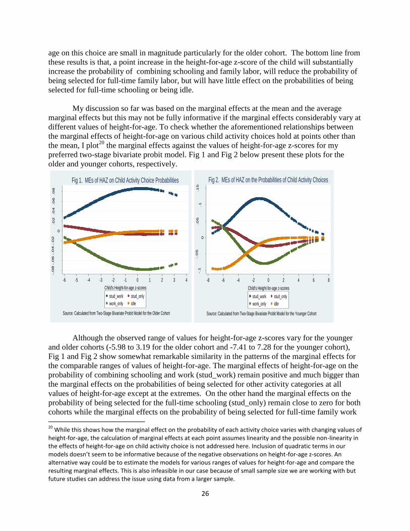
26

age on this choice are small in magnitude particularly for the older cohort. The bottom line from

these results is that, a point increase in the height-for-age z-score of the child will substantially

increase the probability of combining schooling and family labor, will reduce the probability of

being selected for full-time family labor, but will have little effect on the probabilities of being

selected for full-time schooling or being idle.

My discussion so far was based on the marginal effects at the mean and the average

marginal effects but this may not be fully informative if the marginal effects considerably vary at

different values of height-for-age. To check whether the aforementioned relationships between

the marginal effects of height-for-age on various child activity choices hold at points other than

the mean, I plot20

the marginal effects against the values of height-for-age z-scores for my

preferred two-stage bivariate probit model. Fig 1 and Fig 2 below present these plots for the

older and younger cohorts, respectively.

Although the observed range of values for height-for-age z-scores vary for the younger

and older cohorts (-5.98 to 3.19 for the older cohort and -7.41 to 7.28 for the younger cohort),

Fig 1 and Fig 2 show somewhat remarkable similarity in the patterns of the marginal effects for

the comparable ranges of values of height-for-age. The marginal effects of height-for-age on the

probability of combining schooling and work (stud_work) remain positive and much bigger than

the marginal effects on the probabilities of being selected for other activity categories at all

values of height-for-age except at the extremes. On the other hand the marginal effects on the

probability of being selected for the full-time schooling (stud_only) remain close to zero for both

cohorts while the marginal effects on the probability of being selected for full-time family work 20

While this shows how the marginal effect on the probability of each activity choice varies with changing values of height-for-age, the calculation of marginal effects at each point assumes linearity and the possible non-linearity in the effects of height-for-age on child activity choice is not addressed here. Inclusion of quadratic terms in our models doesn’t seem to be informative because of the negative observations on height-for-age z-scores. An alternative way could be to estimate the models for various ranges of values for height-for-age and compare the resulting marginal effects. This is also infeasible in our case because of small sample size we are working with but future studies can address the issue using data from a larger sample.

-.08

-.06

-.04

-.02

0

.02

.04

.06

.08

Margin

al E

ffects

-6 -5 -4 -3 -2 -1 0 1 2 3 4

Child's Height-for-age z-scores

stud_work stud_only

work_only idle

Source: Calculated from Two-Stage Bivariate Probit Model for the Older Cohort

Fig 1. MEs of HAZ on Child Activity Choice Probabilities

-.1

-.0

5

0

.0

5.1

.1

5

Ma

rg

ina

l E

ffe

cts

-8 -6 -4 -2 0 2 4 6 8

Child's Height-for-age z-scores

stud_work stud_only

work_only idle

Source: Calculated from Two-Stage Bivariate Probit Model for the Younger Cohort

Fig 2. MEs of HAZ on the Probabilities of Child Activity Choices

27

(work_only) remain mostly negative. The patterns in the marginal effects of height-for-age on

the probability of being idle appear to differ for the two cohorts at smaller values of height-for-

age but the overall pattern is similar here as well. Therefore, the relationship between the

marginal effects we observed at the mean of height-for-age is not limited to that particular point

but holds throughout except at the extremes where we have only a few observations and hence

all the marginal effects approach zero. In fact my conclusion based on the marginal effects at the

mean or the average marginal effects seems to be reasonable since most of the marginal effects

are clustered around the marginal effects at the mean as demonstrated by their Epanechnikov

kernel densities21

presented in Figs 3-6 for the older cohort and Figs 7-10 for the younger

cohort.

21

The "optimal" width is used in constructing each of the kernel densities for the MEs. The optimal width is the width that would minimize the mean integrated squared error.

050

10

015

020

025

030

035

0

-.008 -.006 -.004 -.002 0 .002 .004 .006 .008 .01

Density kdensity stud_only

Fig 3. MEs of Height-for-age on p(stud=1, work=0): Older Cohort

020

40

60

80

10

0

.02 .03 .04 .05 .06 .07 .08 .09

Density kdensity stud_work

Fig 4. MEs of Height-for-age on p(stud=1, work=1): Older Cohort

28

Source: Calculated from Two-Stage Bivariate Probit Model for Schooling and Work for

the Older Cohort.

Notes: MEs stands for marginal effects and p stands for probability.

010

20

30

40

50

60

70

-.08 -.07 -.06 -.05 -.04 -.03 -.02 -.01

Density kdensity work_only

Fig 5. MEs of Height-for-age on p(stud=0, work=1): Older Cohort

020

40

60

80

10

012

0

-.025 -.02 -.015 -.01 -.005 0

Density kdensity idle

Fig 6. MEs of Height-for-age on p(stud=0, work=0): Older Cohort0

10

20

30

40

50

60

70

80

-.03 -.02 -.01 0 .01 .02 .03

Density kdensity stud_only

Fig 7. MEs of Height-for-age on p(stud=1, work=0): Younger Cohort

010

20

30

40

50

60

70

80

0 .02 .04 .06 .08 .1 .12

Density kdensity stud_work

Fig 8. MEs of Height-for-age on p(stud=1, work=1): Younger Cohort

29

Source: Calculated from Two-Stage Bivariate Probit Model for Schooling and Work for

the Younger Cohort.

Notes: MEs stands for marginal effects and p stands for probability.

With the exception of the kernel densities of marginal effects of height-for-age on the

probability of being idle that are based on relatively smaller number of observations (Fig 6 for

the older cohort and Fig 10 for the younger cohort), all the other kernel densities are clearly uni-

modal and highly skewed with the bulk of the marginal effects clustered around the marginal

effect at the mean that itself is close to the mode of the distribution in each case. For example,

the marginal effect at the mean of height-for-age on the probability of combining schooling and

family work is 0.075 for the older cohort and 0.113 for the younger cohort in the two-stage

bivariate probit models as shown in tables 1 and 2, respectively. The corresponding average

marginal effects are 0.062 and 0.08 as shown in tables A6 and A7 in Appendix A for the older

and younger cohorts, respectively. The mode of the distribution for the corresponding marginal

effects is about 0.085 for the older cohort (Fig 4) and about 0.118 for the younger cohort (Fig 8)

around which the bulk of the marginal effects are lumped. The same is more or less true for the

marginal effects of height-for-age on the probabilities of being selected for full time schooling

and full-time family labor. That is why the average marginal effects reported in tables A6 and A7

in appendix A and the marginal effects at the mean are not very far apart. Hence, the conclusions

I arrived at on the basis of the marginal effects at the mean of height-for-age seem to be

reasonable.

To get some feel about the validity of the bivariate probit parametric form for the joint

distribution of the errors in the schooling and work equations, I tried to re-estimate the bivariate

models following Gallant and Nychka‘s (1987) semi-nonparametric approach previously

described. Strict application of their approach requires estimating the models for successively

increasing order of the Hermite polynomial and testing the superiority of a lower order against

higher order using likelihood-ratio tests or by model-selection criteria such as the Akaike

information criterion or the Bayesian information criterion. With the relatively small sample of

observations, however, I could hardly obtain convergence for the non-concave pseudo–log-

010

20

30

40

50

-.08 -.06 -.04 -.02 0 .02 .04 .06

Density kdensity work_only

Fig 9. MEs of Height-for-age on p(stud=0, work=1): Younger Cohort

05

10

15

20

-.1 -.09 -.08 -.07 -.06 -.05 -.04 -.03 -.02 -.01 0

Density kdensity idle

Fig 10. MEs of Height-for-age on p(stud=0, work=0): Younger Cohort

30

likelihood function with Hermite polynomials of more than 2 degrees. For the older cohort the

pseudo–log-likelihood function for the two stage model failed to converge even when I set the

order of the polynomial at 2 for both schooling and work equations but it converged when I set

either r1 or r2 to 1. Fig 11 depicts the error densities from the two stage model for the older

cohort when r1=2 and r2=1 while Fig 12 presents the error densities from the two-stage model for

the younger cohort when the order of the Hermite polynomial for both equations is set to 2. The

detailed characteristics of these densities along with the estimated coefficients for the covariates

are presented in table A8 in appendix A.

In the cases where convergence was obtained, the error densities are symmetric and do

not seem to substantially deviate from a normal distribution (in reds) with similar first and

0.1

.2.3

.4

Mar

gina

l Den

sity

of E

rror

s

-5 -4 -3 -2 -1 0 1 2 3 4 5

Child Schooling Equation

0.1

.2.3

.4

Mar

gina

l Den

sity

of E

rror

s

-5 -4 -3 -2 -1 0 1 2 3 4 5

Child Work Equation

Note: The Order of Hermite Polynomials was 2 for Schooling and 1 for Work.

Fig 11. Error Densities from Semi-nonparametric Estimation (2-Stage, Older Cohort)

0.1

.2.3

.4

Marg

ina

l Den

sity

of

Err

ors

-5 -4 -3 -2 -1 0 1 2 3 4 5

Child Schooling Equation

0.1

.2.3

.4

Marg

ina

l Den

sity

of

Err

ors

-5 -4 -3 -2 -1 0 1 2 3 4 5

Child Work Equation

Note: The Order of Hermite Polynomials was 2 for both Schooling and Work Equations.

Fig 12. Error Densities from Semi-nonparametric Estimation (2-Stage,Younger Cohort)

31

second moments as demonstrated in Fig 11 and Fig 12 for the older and the younger cohorts,

respectively. The measures of skewness and kurtosis reported in table A8 in appendix A are

consistent with this observation. Although the magnitudes of the coefficient estimates from the

semi-nonparametric models are not directly comparable to those from the bivariate probit model

since the former depend on the normalization of the coefficients of the Hermite polynomials, the

signs and statistical significances of the coefficients are generally consistent with the exception

of the two-stage equation for the child work for the older cohort. Given the symmetry of the error

densities and qualitative resemblance in the estimated coefficients, therefore, the bivariate probit

model doesn‘t seem to be unreasonable for my data.

Finally, I tried to check if my results for the younger cohort are being driven by the

replacement of the missing monthly rainfall records with their long-term averages by re-

estimating the models for the younger cohort, successively excluding the major cases with

missing rainfall records from my estimation sample. The results from this exercise for my

preferred bivariate probit model are reported in table B3 in appendix B. The corresponding first-

stage results and marginal effects are reported in tables B4 and B5, respectively. The first

adjustment I make is to limit my estimation sample to those who had at least 6 months of non-

missing rainfall records including the main rainy (agricultural) season in the locality for at least 1

of the three critical years of development. The next adjustment I make is to limit my estimation

sample to those who fulfill the same condition as in the first adjustment for at least 2 of the three

critical years of development. And finally I limit my estimation sample to those who fulfill the

same condition for all the three critical years of development. These adjustments produce little

changes in the signs, magnitudes and qualities of the first-stage results, the coefficient estimates

and the corresponding marginal effects as shown in the appendix. For example, I lose 283

observations because of the final adjustment but the marginal effect at the mean of height-for-age

on p(stud=1, work=1) decreases from 0.113 to 0.106, its marginal effect on p(stud=1, work=0)

decreases from -0.013 to -0.016, the marginal effect on p(stud=0, work=1) increases from -0.064

to -0.055 and the marginal effect on p(stud=0, work=0) increases from -0.038 to -0.036. While I

still kept some cases with smaller number of missing rainfall records in my estimation sample, if

there was a major understatement of my estimates because of the missing rainfall records it is

likely that larger changes in the estimates would have been observed when I removed all the

major cases with missing rainfall records. Hence, it doesn‘t seem that my results for the younger

cohort are being driven by the replacement of the missing rainfall records by their long-term

averages.

In general, therefore, the findings from both the older and younger cohort indicate that

better access to early childhood nutrition can improve the child‘s prospects for attending

schooling but may also put the child in additional pressure to participate in family labor

activities. This may take the form of asking the child to miss classes in order to help with family

labor activities at home, for example, when agricultural activities are at their peak during

harvesting season or the child may be asked to look after the livestock or fetch drinking water or

fuel wood after coming back from school or during the weekends. While the data at hand do not

contain information on the child‘s performance at school and hence do not allow analysis of how

performance may be affected by the child‘s physical stature, it is quite possible that the

additional pressure put on the child‘s time from the family labor activities could constrain the

amount of time the child could spend on home works and other school related activities at home

and hence lead to poor performance at school. Therefore, policies that try to promote schooling

32

through nutrition support programs could be more effective if they are accompanied by programs

(such as income support schemes) that could mitigate the forces that push families to resort to

child labor.

6. Conclusion

This paper examines how malnutrition experienced during early childhood influences the

subsequent participation of the child in schooling and child labor activities in rural Ethiopia. The

cumulative outcome of the child‘s early childhood nutritional experience is measured by the

child‘s height-for-age z-score which is also taken as a measure of the child‘s physical fitness. My

theoretical model implies that the effect of the child‘s physical fitness on the parental choice as

to whether to select the child for schooling or child labor is ambiguous. Bivariate probit as well

as separate probit models are estimated to empirically examine the effect of the child‘s physical

fitness on his/her participation in schooling and family labor activities. Data from various rounds

of a unique longitudinal rural household survey in Ethiopia (Ethiopian Rural Household Survey)

are used to estimate the models. To address the potential endogeneity of the child‘s physical

fitness in the models for child activity choices, I estimate the models in two-stages. Exposure to a

famine caused by a massive drought in 1984 is used as an exogenous source of early childhood

malnutrition for the older cohort of children for whom the models were estimated. Localized

rainfall shocks were used as a source of identification for the younger cohort of children for

whom a separate set of estimates were obtained.

The first stage results show that exposure to significant weather shocks during the first

three years of the child‘s life generally have a lasting negative effect on his/her age standardized

heights measured later in life. The effect is particularly strong when the child is exposed to the

shock during his/her second year. Estimation results from the child‘s activity choice models

indicate that better early childhood nutrition enhances the child‘s chances of attending school

later in the child‘s life. The range of marginal effects obtained from the two stage bivariate

probit models imply that equalizing the median height of the children in the sample for the two

cohorts with the heights of healthy American children of the same age through better nutrition

and care in the early childhood would boost the chances of school attendance among the children

by at least 14% and possibly by as much as 20%.

On the other hand, I find no conclusive evidence that better physical fitness of the child

leads to his/her positive selection for full-time child labor activities. I rather found reasonably

strong and consistent evidence that physically robust children are more likely to combine child

labor and schooling than physically weaker children. The results are consistent across two

different cohorts of children and two different identification strategies. The findings indicate

that, although better early childhood nutrition leads to higher chances of attending school, it may

also put the child at additional pressure to participate in family labor activities and this may be

reflected in poor performance in schooling. Therefore, policies that try to promote schooling

through nutrition support programs could be more effective if they are accompanied by programs

that could mitigate the forces that push families to resort to child labor. My next work in this area

will look at how the observed effect of physical fitness on the probability of combining child

labor and schooling affects the child‘s school performance in the form of test scores and grades.

33

REFERENCES

Alderman, H. and Hoddinott, J. and Kinsey, B. 2006. ―Long Term Consequences of Early

Childhood Malnutrition,‖ Oxford Economic Papers, Vol. 58, No.3, pp.450-474.

Angrist, J. and W. Evans.1998. ―Children and Their Parents‘ Labor Supply: Evidence from

Exogenous Variation in Family Size,‖ The American Economic Review, 88(3), pp.450-

477.

Bacolod, Marigee P. and Priya Ranjan. 2008. ―Why Children Work, Attend School, or Stay Idle:

The Roles of Ability and Household Wealth,‖ Economic Development and Cultural

Change, Vol. 56, pp.791-828.

Barro, Robert J. and Gary S. Becker. 1989. ―Fertility Choice in a Model of Economic Growth‖,

Econometrica, Vol. 57, No.2, pp.481-501.

Baser, O., Bradley, C.J., Gardiner, J.C., Given, C., 2004. Testing and correcting for non-random

selection bias due to censoring: an application to medical costs. Health Services and

Outcomes Research Methodology 4, 93–107.

Binder, M. 1999. ―Schooling Indicators during Mexico‘s ‗Lost Decade.‘‖ Economics of

Education Review, 18(2):183–99.

Bourguignon, F., F. Ferreira, and P. Leite. 2003. ―Conditional Cash Transfers, Schooling, and

Child Labor: Micro-Simulating Brazil‘s Bolsa Escola Program.‖ World Bank Economic

Review, 17(2):229–54.

Cameron, A.Colin and Pravin K. Trivedi.2005. Microeconometrics: Methods and Applications,

Cambridge.

Carlin, John B., Lyle C. Gurrin, Jonathan AC Sterne, Ruth Morley, and Terry Dwyer. 2005.

Carter, R. Michael. and Maluccio, A. John. 2003. ―Social Capital and Coping with Economic

Shocks: An Analysis of Stunting of South African Children‖, World Development,

Vol.31, No.7, pp.1147-1163.

Cigno, Allessandro, and Furio Rosati. 2005. The economics of child labour. New York: Oxford

University Press.

Dammert, Ana. 2008. ―Child Labor and Schooling Responses to Changes in Coca Production in

Rural Peru,‖ Journal of Development Economics, Vol.86, pp.164-180.

Dasgupta, Partha. 1997. "Nutritional Status, the Capacity for Work and Poverty Traps." Journal

of Econometrics 77(1): 5-38.

De Luca, Giuseppe. 2008. ―SNP and SML estimation of univariate and bivariate binary-choice

models,‖ The State Journal, Vol. 8, No. 2, pp. 190–220.

34

Dercon, Stefan.2004. ―Growth and Shocks: Evidence from Rural Ethiopia,‖ Journal of

Development Economics,‖ Vol.74, pp.309-329.

Dercon, Stefan. 2000. ―Changes in Poverty and Social Indicators in Ethiopia in the 1990s,‖

Oxford University, Centre for the Study of African Economies (CSAE), Oxford

University.

Dercon, S. and P.Krishnan.2000. ―Vulnerability, seasonality and poverty in Ethiopia‖, Journal of

Development Studies, vol.36, no.6. pp.25-53.

DeSimone, J., 2002. ―Illegal drug use and employment‖. Journal of Labor Economics 20, 952–

977.

Duflo, E. 2003. ―Grandmothers and Granddaughters: Old-Age Pensions and Intra-household

Allocation in South Africa.‖ World Bank Economic Review, 17(1):1–25.

Dillon, Andrew.2008. ―Child Labor and Schooling Responses to Production and Health Shocks

in Northern Mali,‖ IFPRI Discussion Paper 00755.

Edmonds, Eric, 2006. ―Child labor and schooling responses to anticipated income in South

Africa,‖ Journal of Development Economics, 81 (2), 386–414.

Emerson, P., and A.P. Souza. 2007. ―Child Labor, School Attendance, and Intrahousehold

Gender Bias in Brazil.‖ World Bank Economic Review, 21(2), pp.301–16.

Gibson, T.B., Mark, T.L., Axelsen, K., Baser, O., Rublee, D.A., McGuigan, K.A., 2006. ―Impact

of statin copayments on adherence and medical care utilization and expenditures‖.

American Journal of Managed Care, 12, SP11–SP19.

Glewwe, Paul .2002. ―Schools and skills in developing countries: Education policies and

socioeconomic outcomes Source‖ Journal of Economic Literature, vol:40(2), pp. 436-

482.

Glewwe, Paul and Hanan Jacoby, 1995, ―An economic analysis of delayed primary school

enrollment and childhood malnutrition in a low income country‖ Review of Economics

and Statistics, vol. 77, pp. 156-169.

Glewwe, Paul and Elizabeth King, 2001, ― The Impact of Early Childhood Nutritional

Status on Cognitive Development: Does the Timing of Malnutrition Matter? ― World

Bank Economic Review 15(1):81-114.

Glewwe, Paul, Hanan Jacoby and Elizabeth King, 2001, ―Early childhood nutrition and

academic achievement: A longitudinal analysis‖, Journal of Public Economics 81(3):

345-368.

Golden, MH.1994. ―Is Complete Catch-up Possible for Stunted Malnourished Children?‖

European Journal of Clinical Nutrition, Vol.48, Suppl.1, S58-70.

35

Gramm, M., 2003. ―The case for regulatory rent-seeking: CRA based protests of bank mergers

and acquisitions.‖ Public Choice, 116, 367–379.

Greene, W.H., 2007. Econometric Analysis, 6th ed. Prentice Hall, Upper Saddle River, NJ.

Haddad, L., & Hoddinott, J. 1994. ―Women‘s income and boy–girl anthropometric status in the

Côte d‘Ivoire,‖ World Development, Vol. 22, 543–553.

Hausman, J. 1975. ―An Instrumental Variable Approach to Full Information Estimators for

Linear and Certain Nonlinear Econometric Models‖, Econometrica, Vol. 43, No. 4 , pp.

727-738.

Hoddinott, John and Kinsey Bill. 2001. ―Child Growth in the time of Drought‖, Oxford Bulletin

of Economics and Statistics, Vol. 63, No.4, pp.409-436.

Jansen, Kurt, M. Harris, and M. Penrose. 1987. The Ethiopian Famine. London: Zed Press.

Kruger, Diana I. 2007. ―Coffee production effects on child labor and schooling in rural Brazil.‖

Journal of Development Economics, 82 (2): 448-463.

Lu, M., McGuire, T.G., 2002. ―The productivity of outpatient treatment for substance abuse.‖

Journal of Human Resources 37, 309–335.

Maccini, S. and Yang, D. 2008. ― Under the Weather: Health, Schooling and Economic

Consequences of Early-Life Rainfall‖, American Economic Review, Vol. 99, No. 3, pp.

1006–1026.

Maitra, Pushkar and Ranjan Ray.2002. ―The Joint Estimation of Child Participation in Schooling

and Employment: Comparative Evidence from Three Countries,‖ Oxford Development

Studies, Vol.30, No.1, pp.41-62.

Martorell, Reynaldo.1999. ―The nature of child malnutrition and its long-term implications‖

Food and Nutrition Bulletin, vol. 19, pp. 288-292.

Martorell, Reynaldo .1997. ―Under nutrition during pregnancy and early childhood and its

consequences for cognitive and behavioral development‖ in M.E. Young (ed) Early

childhood development: Investing in our children’s future (Elsevier: Amsterdam).

Martorell, Reynaldo, Dirk G. Schroeder, Juan A. Rivera and Haley J. Kaplowitz. 1995. ―Patterns

of Linear Growth in Poor Guatemalan Adolescents and Children,‖ The Journal of

Nutrition, 125(4S), 1060S-1067S.

Meer, J., Rosen, H.S., 2004. Insurance and the utilization of medical services. Social Science in

Medicine 58, 1623–1632.

Patrinos, A. Harry and Psacharopoulos, G. 1997. ―Family Size, Schooling and Child Labor in

Peru-an Empirical Analysis,‖ Journal of Population Economics, 10: 289-294.

36

Porter, Catherine22

. 2007. ―Long-term Consequences of Severe Shocks in Childhood: Evidence

from the Ethiopian Famine of 1984,‖ Center for the Study of African Economies,

Economics Department, Oxford University.

Rahmato, Dessalegn. 1988. Peasant Survival Strategies. Geneva: International Institute for Relief

and Development/Food for Hungry International.

Ravallion, Martin, and Quentin Wodon. 2000. ―Does Child Labor Displace Schooling? Evidence

on Behavioral Responses to an Enrollment Subsidy.‖ Economic Journal, Vol. 110, no.

462:C158–C175.

Savage, E., Wright, D.J., 2003. ―Moral hazard and adverse selection in Australian private

hospitals: 1989–1990.‖ Journal of Health Economics 22, 331–359.

Shafik, M. Najeeb.2007. ―Household Schooling and Child Labor Decisions in Rural

Bangladesh,‖ Journal of Asian Economics, Vol. 18, pp.946-966.

Schultz, T. 1990. ―Testing the Neoclassical Model of Family Labor Supply and Fertility.‖

Journal of Human Resources, Vol. 25, No. 4, pp.599–634.

Shea, D., Terza, J., Stuart, B., Briesacher, B., 2007. Estimating the effects of prescription drug.

Coverage for medicare beneficiaries. Health Services Research 43, 933–949.

Shin, J., Moon, S., 2007. ―Do HMO plans reduce health care expenditure in the private sector.‖

Economic Inquiry , 45, 82–99.

Smith, L., and L. Haddad. 2000. ―Explaining child malnutrition in developing countries. A cross-

country analysis.‖ Research Report 111. Washington, D.C.: International Food Policy

Research Institute

Stuart, Bruce C., Jalpa A. Doshi, and Joseph V. Terza .2009. ―Assessing the Impact of Drug Use

on Hospital Costs.‖ Health Services Research, Vol., Number 1, pp. 128-144.

Terza, V. Joseph, Anirban Basu and Paul J. Rathouz. 2008. ―Two-stage residual inclusion

estimation: Addressing endogeneity in health econometric modeling.‖ Journal of Health

Economics, 2008, vol. 27, issue 3, pp.531-543.

Thomas, D. 1990. ―Intra-household Allocation: An Inferential Approach.‖ Journal of Human

Resources, 25(4):635–64.

———.1997. ― Incomes, expenditures, and health outcomes: Evidence on intra-household

resource allocation.‖ In Intra-household resource allocation: Methods, models, and

policy, ed. L. Haddad, J. Hoddinott, and H. Alderman. Baltimore, Md., U.S.A.: Johns

Hopkins University Press for the International Food Policy Research Institute.

Townsend, R. 1995. ―Consumption Insurance: An Evaluation of Risk Bearing Systems in Low

Income Countries‖, Journal of Economic Perspectives, Vol.9, pp.83-102.

22

The author requested that the document should not yet be quoted.

37

Webb, Patrick., Braun, von Joachim and Yisehac Yohannes. 1992. Famine in Ethiopia: Policy

Implications of Coping Failure at the National and Household Level, International Food

Policy Research Institute, Research Report 92.

Wooldridge, M. Jeffrey. 2002. Econometric Analysis of Cross Section and Panel Data, The MIT

Press, Cambridge Massachusetts.

38

APPENDICES

Appendix A. Summary Statistics and Additional Results

Table A1. Summary Statistics for the Variables Used in the Econometric Models for the

Older Cohort

1994a

(Obs=1232)

1995

(Obs=1116)

Variable Description Mean St.dev Mean St.dev

Student dummy=1 if student at school 0.24 0.43 0.34 0.48

Working dummy=1 if working

0.89 0.31

Neither a student nor working dummy=1 if neither student at

school nor working 0.07 0.26 0.02 0.13

Student Only dummy=1 if student at school

and not working

0.09 0.29

Work only dummy=1 if working and not 0.69 0.46 0.64 0.48

student at school

Student and working dummy=1 if student at school

and working

0.25 0.44

Child activity activity=0 if idle, =1 if student

only , =2 if work only, =3 if student

and working

2.13 0.63

Main activity of child main activity=0 if idle, =1 if

student, =2 if working 1.61 0.62 1.62 0.51

Sex sex=1 if male 0.51 0.50 0.51 0.50

Age Age 12.40 1.76 13.10 1.63

Agri. land area owned Agricultural land area owned 1.87 1.76 2.12 2.15

Livestock units owned Tropical livestock units owned 4.89 6.68 4.77 6.35

Father's education dummy=1 if child's father has

completed at least primary

education 0.08 0.27 0.08 0.28

Mother's education dummy=1 if child's mother has

completed at least primary

education 0.02 0.14 0.02 0.13

Distance to primary school Distance to the nearest primary

school in kilometers 6.00 4.27 6.16 4.40

Household size Household Size 8.26 3.24 8.73 3.39

Number of siblings Number of siblings of the child 5.04 2.85 5.28 2.93

Age of father Age of child's father 49.30 9.82 49.93 9.93

Age of mother Age of child's mother 40.05 8.43 40.81 8.61

Sex of household head dummy=1 if h.hold head is male 0.82 0.39 0.81 0.39

Drought Affected in 1984 dummy=1 if household lost crop

and/or livestock because of 1984

39

drought 0.60 0.49 0.62 0.48

First Year in 1984 dummy=1 if child was in his/her

first year in 1984 0.20 0.40 0.23 0.42

Second Year in 1984 dummy=1 if child was in his/her

second year in 1984 0.14 0.35 0.17 0.37

Third Year in 1984 dummy=1 if child was in his/her

third year in 1984 0.19 0.39 0.21 0.41

Drought Affected at 1st Year dummy=1 if child was in 1st year

IN 1984 and belonged to drought

affected household 0.12 0.32 0.14 0.35

Drought Affected at 2nd Year dummy=1 if child was in 2nd year

in 1984 and belonged to drought

affected household 0.09 0.28 0.11 0.31

Drought Affected at 3rd Year dummy=1 if child was in 3nd year

in 1984 and belonged to drought

affected household 0.12 0.33 0.14 0.34

Height-for-age Child's Height-for-age z-scores -1.96 1.54 -2.12 1.44

Height-for-age(Dr84) Obs.94=742, Obs.95 =697 -1.99 1.52 -2.11 1.47

Height-for-age (No Dr84) Obs.94=490, Obs.95 =419 -1.91 1.55 -2.15 1.38

Height-for-age(Dr84, A1-3) Obs.94=406, Obs.95 =426 -1.93 1.60 -2.05 1.48

Height-for-age (No Dr84, A1-3 ) Obs.94=259, Obs.95 =249 -1.75 1.61 -1.98 1.39

Height-for-age(Dr84, A4-6) Obs.94=336, Obs.95 =271 -2.07 1.44 -2.21 1.65

Height-for-age (No Dr84, A4-6 ) Obs.94=231, Obs.95 =170 -2.09 1.42 -2.39 1.35

Height of mother Height of mother in centimeters 156.7 7.31 156.8 5.71

Height of father Height of father in centimeters 168.2 5.35 165.9 7.84

Source: Ethiopian Rural Household Survey.

Notes: Dr84 identifies children affected by the 1984 drought; A1-3 identifies children who were 1

to 3 years old at the time of the 1984 drought while A4-6 identifies children who were age 4 to 6

at the time; Obs.94/Obs.95 stand for the number of observations in the category during the

1994a/1995 rounds.

Table A2. Summary Statistics for the Variables Used in the Econometric Models for the

Younger Cohort

1999

(Obs=1184)

2004

(Obs=1057)

Variable Description Mean St.dev Mean St.dev.

Student dummy=1 if student at school 0.32 0.47 0.70 0.46

Student Only dummy=1 if student at school

and not working 0.14 0.35 0.13 0.33

Working dummy=1 if working 0.65 0.48 0.86 0.34

Work only dummy=1 if working and not

student at school 0.48 0.50 0.29 0.45

Student and working dummy=1 if student at school

and working 0.17 0.38 0.57 0.49

40

Neither student nor working dummy=1 if neither student at

school nor working 0.21 0.40 0.01 0.12

Main activity of child main activity=0 if idle, =1 if

student, =2 if working 1.27 0.78 1.28 0.48

Child activity activity=0 if idle, =1 if student

only, =3 if work only,=3 if

student and working 1.62 1.00 2.42 0.76

Child's Height-for-age Child's Height-for-age z-scores -2.22 2.06 -2.25 2.04

Sex sex=1 if male 0.50 0.50 0.52 0.50

Age Age 8.24 1.77 13.24 1.77

Household size Household Size 8.83 3.49 7.20 2.35

Number of siblings Number of siblings of the child 4.45 2.08 4.66 2.14

Sex of household head dummy=1 if h.hold head is male 0.81 0.39 0.79 0.41

Father's education dummy=1 if child's father has

completed at least primary

education 0.17 0.38 0.18 0.38

Mother's education dummy=1 if child's mother has

completed at least primary

education 0.05 0.22 0.06 0.23

Distance to primary school Distance to the nearest primary

school in kilometers 4.69 3.67 3.74 3.04

Age of father Age of child's father 47.96 10.97 52.81 11.01

Age of mother Age of child's mother 37.92 8.42 42.80 8.32

Agri. Land area owned Agricultural land area owned 1.46 1.40 1.44 1.70

Livestock units owned Tropical livestock units owned 4.08 4.03 6.21 7.57

Rainfall deviation at 1st year Deviation of rain from long run

local mean during 1st year 21.89 171.13 22.50 172.69

Rainfall deviation at 2nd year Deviation of rain from long run

local mean during 2nd year -3.66 160.23 -2.51 152.11

Rainfall deviation at 3rd year Deviation of rain from long run

local mean during 3rd year -23.58 169.76 -21.53 164.68

Substantial rain def. at 1st year dummy=1 if rain deficit at 1st

year exceeds local st.dev 0.13 0.33 0.12 0.32

Substantial rain def. at 2nd year dummy=1 if rain deficit at 2nd

year exceeds local st.dev 0.17 0.38 0.16 0.37

Substantial rain def. at 3rd year dummy=1 if rain deficit at 3rd

year exceeds local st.dev 0.20 0.40 0.19 0.39

Substantial rain sur. at 1st year dummy=1 if rain surplus at 1st

year exceeds local st.dev 0.13 0.33 0.13 0.33

Substantial rain sur. at 2nd year dummy=1 if rain surplus at 2nd

year exceeds local st.dev 0.12 0.32 0.11 0.32

Substantial rain sur. at 3rd year dummy=1 if rain surplus at 3rd

year exceeds local st.dev 0.09 0.28 0.09 0.29

41

Height of mother Height of mother in centimeters 156.57 6.44 156.45 6.56

Height of father Height of father in centimeters 166.23 7.90 166.20 7.80

Source: Ethiopian Meteorological agency for the rainfall data, Ethiopian Rural

Household Survey for all the Other Variables.

Table A3. The Effect of Exposure to Drought and Rainfall Fluctuations in Early

Childhood on Height-for-age Z- scores (First Stage Results) Older Cohort Younger Cohort

I

(94a&95)

II

(1995)

III

(94a&95)

IV

(99&04)

V

(99&04)

Drought Affected in 1984 0.171 0.294* 0.170

(0.151) (0.173) (0.151)

First Year in 1984 0.129 0.242 -0.058

(0.303) (0.366) (0.228)

Second Year in 1984 0.462* 0.431 0.322

(0.261) (0.311) (0.214)

Third Year in 1984 -0.202 -0.106 -0.294*

(0.199) (0.224) (0.171)

Drought Affected at 1st Year -0.094 -0.077 -0.094

(0.202) (0.216) (0.201)

Drought Affected at 2nd Year -0.592*** -0.487** -0.590***

(0.227) (0.246) (0.227)

Drought Affected at 3rd Year 0.098 -0.055 0.098

(0.193) (0.207) (0.193)

Substantial rain def. at 1st year 0.047 0.061

(0.223) (0.220)

Substantial rain def. at 2nd year -0.401** -0.402**

(0.179) (0.180)

Substantial rain. def. at 3rd year -0.243 -0.237

(0.178) (0.178)

Substantial rain surp. at 1st year -0.030 -0.034

(0.178) (0.178)

Substantial rain surp. at 2nd year -0.227 -0.221

(0.180) (0.179)

Substantial rain surp. at 3rd year -0.094 -0.085

(0.251) (0.250)

Height of Mother 0.023*** 0.024*** 0.023*** 0.028*** 0.028***

(0.007) (0.009) (0.007) (0.010) (0.010)

Height of Father 0.006 0.006 0.007 0.027*** 0.027***

(0.006) (0.008) (0.006) (0.008) (0.008)

Age -0.078 -0.059 -0.125*** -0.020 -0.007

(0.063) (0.083) (0.041) (0.032) (0.017)

Sex -0.229*** -0.171** -0.230*** -0.223* -0.222*

(0.075) (0.081) (0.074) (0.119) (0.118)

Household Size -0.034 -0.023 -0.033 0.016 0.012

(0.022) (0.023) (0.022) (0.025) (0.024)

Number of Siblings 0.053** 0.040 0.052** -0.034 -0.030

(0.024) (0.025) (0.024) (0.035) (0.035)

Sex of Household Head -0.032 -0.026 -0.033 -0.102 -0.102

(0.133) (0.152) (0.133) (0.157) (0.157)

42

Father's Education 0.346* 0.369** 0.338* 0.200 0.203

(0.181) (0.181) (0.181) (0.188) (0.188)

Mother's Education -0.060 -0.164 -0.064 -0.343 -0.340

(0.439) (0.491) (0.438) (0.260) (0.260)

Age of Father 0.004 0.006 0.004 0.004 0.005

(0.005) (0.006) (0.005) (0.008) (0.008)

Age of Mother 0.022*** 0.020*** 0.022*** 0.009 0.009

(0.006) (0.007) (0.006) (0.011) (0.011)

Agri. Land Area Owned 0.005 0.021 0.003 0.003 0.003

(0.024) (0.029) (0.023) (0.032) (0.032)

Livestock Units Owned 0.003 -0.002 0.003 -0.011 -0.010

(0.007) (0.008) (0.007) (0.010) (0.010)

Year=1995 -0.103

(0.069)

Year=2004 0.108

(0.167)

Constant -6.894*** -7.488*** -6.365*** -11.453*** -11.535***

(1.739) (2.149) (1.663) (1.901) (1.873)

F-stat for joint sig of instruments 2.900*** 2.470*** 2.910*** 7.620*** 7.610***

(p=0.005) (p=0.008) (p=0.002) (p=0.000) (p=0.000)

Observations 2348 1116 2348 2241 2241

Cluster-robust standard errors in parentheses

*** p<0.01, ** p<0.05, *p<0.1

Notes: Site dummies were included in all the equations as controls for community fixed effects. Equation

I presents the first stage for the probit models estimated using pooled unbalanced panel data from 1994a

and 1995 rounds. Equation II presents the first stage results for the bivariate probit models estimated

using cross-sectional data from 1995 round. Equation III presents the first stage results for the random

effects probit models estimated using unbalanced panel data from 1994a and 1995 rounds. Equation IV is

the first stage for all the models estimated using pooled panel data for the younger cohort whereas

equation V is the first stage for the random effects probit models for the same cohort. All first stage

equations were separately estimated by OLS and the resulting residuals were used in the second stage

equations as suggested by Terza, Basu and Rathouz (2008).

Table A4. Bivariate Probit Estimates for Child Schooling and Work

Older Cohort Younger Cohort

I II III IV

Biprobit

2-Stage

Biprobit

Biprobit

2-Stage

Biprobit

Student

Child's Height-for-age z-scores 0.121*** 0.199 0.086*** 0.251***

(0.032) (0.223) (0.018) (0.095)

Sex 0.330*** 0.344*** 0.284*** 0.324***

(0.082) (0.090) (0.066) (0.070)

Age 0.040 0.048 0.196*** 0.199***

(0.025) (0.034) (0.018) (0.018)

Agri. Land Area Owned -0.014 -0.016 -0.000 -0.002

(0.030) (0.031) (0.024) (0.024)

Livestock Units Owned 0.011 0.011 0.023*** 0.024***

(0.012) (0.012) (0.008) (0.008)

Father's Educ.-at Least Primary 0.855*** 0.824*** 0.400*** 0.349***

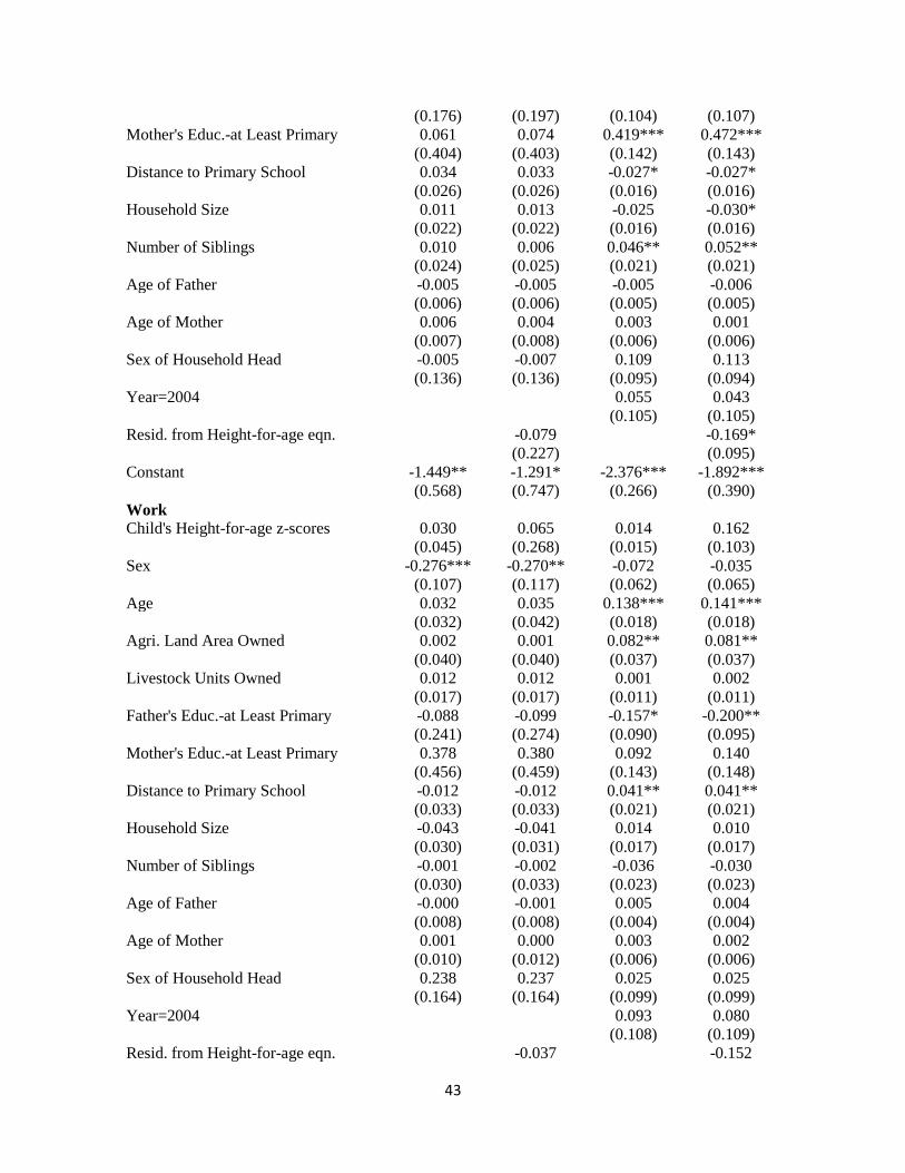
43

(0.176) (0.197) (0.104) (0.107)

Mother's Educ.-at Least Primary 0.061 0.074 0.419*** 0.472***

(0.404) (0.403) (0.142) (0.143)

Distance to Primary School 0.034 0.033 -0.027* -0.027*

(0.026) (0.026) (0.016) (0.016)

Household Size 0.011 0.013 -0.025 -0.030*

(0.022) (0.022) (0.016) (0.016)

Number of Siblings 0.010 0.006 0.046** 0.052**

(0.024) (0.025) (0.021) (0.021)

Age of Father -0.005 -0.005 -0.005 -0.006

(0.006) (0.006) (0.005) (0.005)

Age of Mother 0.006 0.004 0.003 0.001

(0.007) (0.008) (0.006) (0.006)

Sex of Household Head -0.005 -0.007 0.109 0.113

(0.136) (0.136) (0.095) (0.094)

Year=2004 0.055 0.043

(0.105) (0.105)

Resid. from Height-for-age eqn. -0.079 -0.169*

(0.227) (0.095)

Constant -1.449** -1.291* -2.376*** -1.892***

(0.568) (0.747) (0.266) (0.390)

Work

Child's Height-for-age z-scores 0.030 0.065 0.014 0.162

(0.045) (0.268) (0.015) (0.103)

Sex -0.276*** -0.270** -0.072 -0.035

(0.107) (0.117) (0.062) (0.065)

Age 0.032 0.035 0.138*** 0.141***

(0.032) (0.042) (0.018) (0.018)

Agri. Land Area Owned 0.002 0.001 0.082** 0.081**

(0.040) (0.040) (0.037) (0.037)

Livestock Units Owned 0.012 0.012 0.001 0.002

(0.017) (0.017) (0.011) (0.011)

Father's Educ.-at Least Primary -0.088 -0.099 -0.157* -0.200**

(0.241) (0.274) (0.090) (0.095)

Mother's Educ.-at Least Primary 0.378 0.380 0.092 0.140

(0.456) (0.459) (0.143) (0.148)

Distance to Primary School -0.012 -0.012 0.041** 0.041**

(0.033) (0.033) (0.021) (0.021)

Household Size -0.043 -0.041 0.014 0.010

(0.030) (0.031) (0.017) (0.017)

Number of Siblings -0.001 -0.002 -0.036 -0.030

(0.030) (0.033) (0.023) (0.023)

Age of Father -0.000 -0.001 0.005 0.004

(0.008) (0.008) (0.004) (0.004)

Age of Mother 0.001 0.000 0.003 0.002

(0.010) (0.012) (0.006) (0.006)

Sex of Household Head 0.238 0.237 0.025 0.025

(0.164) (0.164) (0.099) (0.099)

Year=2004 0.093 0.080

(0.108) (0.109)

Resid. from Height-for-age eqn. -0.037 -0.152

44

(0.268) (0.105)

Constant 1.207 1.273 -0.897*** -0.467

(0.736) (0.881) (0.258) (0.389)

Athrho

Constant -0.964*** -0.964*** -0.512*** -0.521***

(0.101) (0.101) (0.053) (0.053)

Observations 1116 1116 2241 2241

*** p<0.01, ** p<0.05, * p<0.1 Cluster-robust standard errors in parentheses

Notes: Dummies representing exposure to a big drought in 1984 at 1st, 2

nd and 3

rd years are used as

identifying instruments for child‘s height-for-age in equation (II) . Dummies for substantial rain deficit

and rain surplus at 1st, 2

nd and 3

rd years are used as instruments in (V). Mother‘s height and father‘s height

were also included in all first stage equations to control for genetic variations in height. Site dummies

were included in all equations to control for community fixed effects. The two-stage models are estimated

using the approach suggested by Terza, Basu and Rathouz (2008) as previously discussed.

Table A5. Probit Models for Child Schooling Pooled Panel Panel Pooled Panel Panel

I II III IV V VI VII VII

2-Stage RE 2-Stage

2-Stage RE 2-Stage

Probit Probit Probit

RE

Probit Probit Probit Probit

RE

Probit

Child's Height-for-

age

0.125***

0.276*

0.159***

0.253

0.085***

0.242**

0.105***

0.299**

(0.025) (0.166) (0.035) (0.228) (0.018) (0.097) (0.020) (0.120)

Sex 0.441*** 0.477*** 0.664*** 0.686*** 0.276*** 0.314*** 0.339*** 0.385***

(0.068) (0.078) (0.107) (0.120) (0.066) (0.070) (0.080) (0.085)

Age 0.072*** 0.087*** 0.152*** 0.161*** 0.201*** 0.204*** 0.251*** 0.252***

(0.019) (0.025) (0.030) (0.038) (0.018) (0.018) (0.018) (0.018)

Agri. Land Area

Owned

0.003

0.002

0.027

0.027

-0.001

-0.002

-0.001

-0.002

(0.025) (0.025) (0.033) (0.033) (0.024) (0.024) (0.035) (0.035)

Livestock Units

Owned

0.007

0.006

0.009

0.009

0.022***

0.023***

0.028***

0.029***

(0.009) (0.009) (0.009) (0.009) (0.007) (0.008) (0.009) (0.009)

Father's Education 0.951*** 0.898*** 1.453*** 1.420*** 0.415*** 0.366*** 0.500*** 0.440***

(0.154) (0.163) (0.213) (0.227) (0.106) (0.108) (0.122) (0.126)

Mother's Education 0.055 0.059 0.008 0.011 0.443*** 0.495*** 0.524*** 0.587***

(0.376) (0.374) (0.388) (0.388) (0.144) (0.145) (0.195) (0.199)

Distance to Primary

School

0.034

0.033

0.042

0.041

-0.024

-0.024

-0.034

-0.034

(0.023) (0.024) (0.032) (0.032) (0.015) (0.015) (0.022) (0.022)

Household Size 0.007 0.012 -0.006 -0.003 -0.025 -0.030* -0.029 -0.033*

(0.018) (0.019) (0.026) (0.027) (0.016) (0.016) (0.018) (0.018)

Number of Siblings 0.014 0.005 0.041 0.036 0.048** 0.053** 0.057** 0.063**

(0.020) (0.022) (0.028) (0.030) (0.021) (0.021) (0.025) (0.026)

45

Age of Father -0.002 -0.003 -0.002 -0.002 -0.005 -0.006 -0.007 -0.008

(0.005) (0.005) (0.007) (0.007) (0.005) (0.005) (0.005) (0.005)

Age of Mother 0.003 0.000 0.005 0.003 0.004 0.002 0.005 0.003

(0.005) (0.007) (0.008) (0.009) (0.006) (0.006) (0.007) (0.007)

Sex of Household

Head

0.070

0.073

0.040

0.043

0.124

0.129

0.133

0.138

(0.103) (0.103) (0.145) (0.145) (0.095) (0.094) (0.103) (0.103)

Year=1995 0.331*** 0.345***

(0.056) (0.058)

Year=2004 0.031 0.018

(0.105) (0.105)

Residuals from 1st

stage.

-0.154

-0.096

-0.161*

-0.199*

(0.168) (0.230) (0.097) (0.121)

Constant -2.23*** -1.91*** -3.61*** -3.41*** -2.46*** -2.00*** -3.03*** -2.45***

(0.456) (0.577) (0.698) (0.842) (0.270) (0.393) (0.316) (0.462)

lnsig2u

0.224 0.223 -0.69*** -0.70***

(0.190) (0.190)

(0.264) (0.265)

No. of Individuals

1358 1358

1263 1263

Observations 2348 2348 2348 2348 2241 2241 2241 2241

*** p<0.01, ** p<0.05, * p<0.1

Robust standard errors in parentheses

Notes: Dummies representing exposure to a big drought in 1984 at 1st, 2

nd and 3

rd years are used as

identifying instruments for child‘s height-for-age in (II) &(IV) . Dummies for substantial rain deficit and

rain surplus at 1st, 2

nd and 3

rd years are used as instruments in (VI)&(VIII). Mother‘s height and father‘s

height were also included in all first stage equations to control for genetic variations in height. Site

dummies were included in all the equations to control for community fixed effects.

Table A6. Average Marginal Effects of Child's height-for-age z-scores on the Choice probabilities

of Various Child Activities (Older Cohort)

p(stud=1, p(stud=1, p(stud=0, p(stud=0,

Model p(stud=1|x) work=0|x) work=1|x) work=1|x) work=0|x) p(work=1|x)

Biprobit - 0.001 0.037*** -0.032*** -0.006** -

(0.005) (0.008) (0.009) (0.003)

Biprobit two-stage - 0.001 0.062 -0.052 -0.011 -

(0.036) (0.049) (0.065) (0.017)

Probit 0.036*** - - - - 0.008

(0.007)

(0.007)

Probit, two-stage 0.079* - - - - 0.011

(0.047)

(0.045)

Panel probit 0.034*** - - - - 0.011***

(0.007)

(0.004)

Panel prob. two- stage 0.055 - - - - 0.018

(0.049)

(0.027)

*** p<0.01, ** p<0.05, *p<0.1

46

Notes: Tables A4 and A5 in this appendix respectively present coefficient estimates for bivariate probit and

Probit results from which these partial effects were obtained. The partial effects reported in this table are the

averages of partial effects calculated at each value of the child‘s height-for-age z- scores and the standard errors

were calculated by the delta method. All models included controls for community fixed effects, child age and

sex, land and livestock owned, household size and number of siblings, education of father and mother, distance

to primary school, age of mother and father, and sex of household head.

Table A7. Average Marginal Effects of Child's height-for-age z-scores on the Choice probabilities

of various Child Activities (Younger Cohort)

p(stud=1, p(stud=1, p(stud=0, p(stud=0,

Model p(stud=1|x) work=0|x) work=1|x) work=1|x) work=0|x) p(work=1|x)

Biprobit - 0.005 0.021*** -0.017*** -0.009*** -

(0.003) (0.004) (0.005) (0.002)

Biprobit two-stage - -0.004 0.080*** -0.034 -0.041*** -

(0.019) (0.022) (0.027) (0.014)

Probit 0.026*** - - - - 0.007

(0.005)

(0.015)

Probit, two-stage 0.073** - - - - 0.043

(0.029)

(0.029)

Panel probit 0.029*** - - - - 0.002

(0.005)

(0.004)

Panel probit-two stage 0.082** - - - - 0.040

(0.032)

(0.027)

***p<0.01, ** p<0.05, * p<0.1

Notes: Tables A4 and A5 in this appendix respectively present coefficient estimates for bivariate probit and

Probit results from which these partial effects were obtained. The partial effects reported in this table are the

averages of partial effects calculated at each value of the child‘s height-for-age z- scores and the standard errors

were calculated by the delta method. All models included controls for community fixed effects, child age and

sex, land and livestock owned, household size and number of siblings, education of father and mother, distance

to primary school, age of mother and father, and sex of household head.

Table A8. Semi-Nonparametric Bivariate Estimates for Child Schooling and Work Older Cohort Younger Cohort

Variables

I

SNP

II

2-Stage SNP

III

SNP

IV

2-Stage SNP

Stud

Child's Height-for-age z-scores 0.169*** 0.334 0.097*** 0.304***

(0.042) (0.222) (0.022) (0.100)

Sex 0.468*** 0.499*** 0.353*** 0.410***

(0.105) (0.113) (0.089) (0.103)

Age 0.046 0.066 0.223*** 0.230***

(0.029) (0.043) (0.028) (0.027)

Total Agricultural Land Area Owned -0.031 -0.035 0.010 0.009

(0.038) (0.038) (0.034) (0.034)

47

Total Tropical Livestock Units Owned 0.012 0.013 0.027*** 0.028***

(0.012) (0.012) (0.010) (0.010)

Father's Education-at Least Primary 1.129*** 1.076*** 0.484*** 0.428***

(0.229) (0.237) (0.131) (0.133)

Mother's Education-at Least Primary -0.045 -0.016 0.494** 0.562***

(0.517) (0.514) (0.198) (0.193)

Distance to the Nearest Primary School 0.031 0.036 -0.071*** -0.069***

(0.033) (0.035) (0.022) (0.022)

Household Size 0.034 0.038 -0.030 -0.035

(0.031) (0.031) (0.023) (0.023)

Number of Siblings 0.001 -0.005 0.053* 0.061**

(0.035) (0.036) (0.029) (0.029)

Age of Father -0.006 -0.006 -0.009 -0.009

(0.008) (0.008) (0.007) (0.007)

Age of Mother 0.005 0.002 0.005 0.004

(0.009) (0.009) (0.008) (0.008)

Sex of Household Head -0.032 -0.028 0.125 0.135

(0.168) (0.167) (0.129) (0.129)

year04 0.164 0.139

(0.189) (0.197)

Child's Height-for-age z-scores

Resid. from Height-for-age eqn. -0.168 -0.212**

(0.227) (0.099)

work

Child's Height-for-age z-scores 0.032 -0.369 0.030 0.149

(0.046) (0.269) (0.022) (0.093)

Sex -0.321** -0.390*** -0.072 -0.050

(0.135) (0.144) (0.087) (0.090)

Age 0.131*** 0.061 0.250*** 0.248***

(0.033) (0.051) (0.029) (0.033)

Total Agricultural Land Area Owned 0.008 0.021 0.105** 0.105**

(0.050) (0.050) (0.048) (0.049)

Total Tropical Livestock Units Owned 0.007 0.006 -0.000 0.001

(0.022) (0.022) (0.013) (0.013)

Father's Education-at Least Primary -0.204 -0.104 -0.193 -0.237*

(0.287) (0.312) (0.125) (0.126)

Mother's Education-at Least Primary 0.489 0.437 0.181 0.210

(0.511) (0.518) (0.204) (0.208)

Distance to the Nearest Primary School 0.065** 0.042 0.071** 0.068**

(0.031) (0.034) (0.031) (0.031)

Household Size -0.021 -0.036 0.016 0.012

(0.036) (0.037) (0.023) (0.023)

Number of Siblings -0.009 0.008 -0.041 -0.037

(0.037) (0.040) (0.030) (0.030)

Age of Father 0.001 0.002 0.011** 0.010*

(0.010) (0.010) (0.006) (0.006)

Age of Mother 0.009 0.014 0.004 0.002

(0.012) (0.012) (0.008) (0.008)

Sex of Household Head 0.417** 0.387** 0.106 0.097

48

(0.189) (0.190) (0.135) (0.138)

year04 -0.091 -0.086

(0.210) (0.221)

g_1_1 -0.685*** -0.684*** -0.066 -0.057

(0.042) (0.042) (0.074) (0.088)

g_2_1 0.058** 0.053** 0.270*** 0.268***

(0.023) (0.023) (0.042) (0.042)

g_1_2 -0.225*** -0.225***

(0.023) (0.024)

g_2_2 -0.070*** -0.069***

(0.017) (0.014)

Standard Deviation (s) 1.281 1.281 1.301 1.300

Standard Deviation (w) 1.279 1.279 1.342 1.340

Variance (s) 1.642 1.640 1.692 1.690

Variance(w) 1.636 1.635 1.801 1.796

Skewness(s) -0.072 -0.066 -0.397 -0.395

Skewness(w) -0.005 -0.005 0.331 0.329

Kurtosis(s) 2.550 2.551 3.127 3.124

Kurtosis(w) 2.527 2.531 3.055 3.053

rho -0.557 -0.559 -0.484 -0.482

Observations 1116 1116 2241 2241

Robust standard errors in parentheses

*** p<0.01, ** p<0.05, * p<0.1

Note: The bivariate binary-choice models were estimated through the semi-nonparametric estimators of

Gallant and Nychka (1987). The unknown density of the latent regression errors is approximated by a

Hermite polynomial expansion of order 2 for and 1 for the schooling and work equations for the older

cohort and order 2 in both equations for the younger cohort. Convergence was hard to obtain with higher

order polynomials because of the non-concavity of the log pseudolikelihood function.

Appendix B. Robustness to Missing Rainfall Data

Table B1. Missing Monthly Rainfall Records for the 8 Critical Years in the Analysis of the

Younger Cohort

Year

Site 1988 1989 1990 1991 1992 1993 1994 1995

Adado 3 0 0 5 0 3 0 0

Adele Keke 0 0 0 0 1 12 12 12

Aze Deboa 0 0 0 0 0 0 0 1

Debre berhan 2 0 0 1 0 3 1 1

Dinki 1 0 0 0 0 0 0 0

Doma'a 0 0 0 0 0 0 1 0

Gara Godo 4 1 1 1 2 2 0 0

Geblen 12 12 12 12 5 0 0 0

Haresaw 8 12 12 12 4 0 0 3

Imdibir 0 0 0 0 1 0 12 4

Koro degaga 0 0 0 4 4 2 0 0

Shumsha 0 5 12 12 6 1 0 1

Sirbana Gudeti 0 0 1 4 0 0 1 0

49

Tirufe Kecheme 0 0 0 1 0 0 1 0

Yetmen 0 0 3 0 0 0 0 0

Table B2. Availability of Rainfall Data During the Main Rainy Season

Year

Site 1988 1989 1990 1991 1992 1993 1994 1995

Adado A A A A A A A A

Adele Keke A A A A A NA NA NA

Aze Deboa A A A A A A A A

Debre berhan A A A A A A A A

Dinki A A A A A A A A

Doma'a A A A A A A A A

Gara Godo A A A A A A A A

Geblen NA NA NA NA A A A A

Haresaw NA NA NA NA A A A A

Imdibir A A A A A A NA A

Koro degaga A A A A A A A A

Shumsha A A NA NA A A A A

Sirbana Gudeti A A A A A A A A

Tirufe Kecheme A A A A A A A A

Yetmen A A A A A A A A

Notes: A stands for "data available" and NA stands for "data not available".

Table B3. Two-Stage Bivariate Probit Results-Successively Adjusting the Estimation Sample for the

Major Missing Rainfall Records VARIABLES (I) (II) (III) (IV)

Student

Child's Height-for-age z-scores 0.251*** 0.259*** 0.233** 0.226**

(0.095) (0.095) (0.101) (0.105)

Sex 0.324*** 0.326*** 0.315*** 0.314***

(0.070) (0.070) (0.072) (0.072)

Age 0.199*** 0.199*** 0.200*** 0.210***

(0.018) (0.019) (0.020) (0.021)

Total Agricultural Land Area Owned -0.002 -0.007 -0.006 -0.003

(0.024) (0.023) (0.024) (0.023)

Total Tropical Livestock Units Owned 0.024*** 0.024*** 0.023*** 0.022***

(0.008) (0.008) (0.008) (0.008)

Father's Education-at Least Primary 0.349*** 0.362*** 0.377*** 0.370***

(0.107) (0.107) (0.109) (0.114)

Mother's Education-at Least Primary 0.472*** 0.489*** 0.494*** 0.502***

(0.143) (0.144) (0.148) (0.153)

Distance to the Nearest Primary School -0.027* -0.031** -0.027* -0.026

(0.016) (0.016) (0.016) (0.016)

50

Household Size -0.030* -0.027* -0.030* -0.028

(0.016) (0.017) (0.017) (0.017)

Number of Siblings 0.052** 0.054** 0.056** 0.061***

(0.021) (0.022) (0.022) (0.023)

Age of Father -0.006 -0.007 -0.007 -0.005

(0.005) (0.005) (0.005) (0.005)

Age of Mother 0.001 0.001 0.003 0.002

(0.006) (0.006) (0.006) (0.007)

Sex of Household Head 0.113 0.079 0.077 0.079

(0.094) (0.096) (0.099) (0.105)

Resid. from Height-for-age eqn. -0.169* -0.175* -0.150 -0.141

(0.095) (0.095) (0.100) (0.105)

Year=2004 0.043 0.065 0.069 0.045

(0.105) (0.111) (0.112) (0.115)

Constant -1.892*** -1.965*** -2.059*** -2.229***

(0.390) (0.389) (0.407) (0.416)

Work

Child's Height-for-age z-scores 0.162 0.176* 0.189* 0.174

(0.103) (0.102) (0.106) (0.115)

Sex -0.035 -0.068 -0.098 -0.119*

(0.065) (0.066) (0.068) (0.069)

Age 0.141*** 0.148*** 0.140*** 0.140***

(0.018) (0.019) (0.020) (0.021)

Total Agricultural Land Area Owned 0.081** 0.080** 0.076** 0.073**

(0.037) (0.037) (0.037) (0.037)

Total Tropical Livestock Units Owned 0.002 0.002 0.002 0.002

(0.011) (0.011) (0.011) (0.012)

Father's Education-at Least Primary -0.200** -0.190* -0.177* -0.193*

(0.095) (0.097) (0.099) (0.101)

Mother's Education-at Least Primary 0.140 0.144 0.140 0.128

(0.148) (0.150) (0.153) (0.158)

Distance to the Nearest Primary School 0.041** 0.041** 0.045** 0.045**

(0.021) (0.021) (0.021) (0.021)

Household Size 0.010 0.006 0.006 0.009

(0.017) (0.018) (0.018) (0.019)

Number of Siblings -0.030 -0.031 -0.030 -0.036

(0.023) (0.024) (0.024) (0.025)

Age of Father 0.004 0.004 0.004 0.004

(0.004) (0.004) (0.004) (0.004)

Age of Mother 0.002 0.003 0.003 0.003

(0.006) (0.006) (0.006) (0.006)

Sex of Household Head 0.025 0.087 0.077 0.103

(0.099) (0.103) (0.107) (0.112)

Resid. from Height-for-age eqn. -0.152 -0.169 -0.188* -0.170

(0.105) (0.104) (0.108) (0.117)

Year=2004 0.080 0.015 0.080 0.097

(0.109) (0.114) (0.118) (0.120)

Constant -0.467 -0.355 -0.349 -0.388

(0.389) (0.400) (0.408) (0.422)

Athrho -0.521*** -0.518*** -0.510*** -0.522***

51

(0.053) (0.054) (0.055) (0.057)

Observations 2241 2145 2053 1958

Robust standard errors in parentheses

*** p<0.01, ** p<0.05, * p<0.1

Notes: Site dummies were included in all equations to control for community fixed effects. Equation (I)

was estimated using the entire sample. Equation (II) includes in the estimation sample only those who had

at least 6 months of non-missing monthly rainfall records including the main rainy (agricultural) season

during at least 1 of their critical years of development. The 5 and 6 year olds from Geblen and Haresaw

and 1 year olds from Adele Keke did not fulfill these criteria and were excluded from the estimation

sample for (II). Equation (III) includes in the estimation sample only those who had at least 6 months of

non-missing monthly rainfall records including the main rainy (agricultural) season during at least 2 of

their critical years of development. The 4, 5 and 6 year olds from Geblen and Haresaw, 1 and 2 year olds

from Adele Keke and 4 year olds from Shumsha did not fulfill these criteria and were excluded from the

estimation sample for (III). Equation (IV) includes in the estimation sample only those who had at least 6

months of non-missing monthly rainfall records including the main rainy (agricultural) season for all of

the 3 critical years of development. The 3, 4, 5 and 6 year olds from Geblen and Haresaw, 1, 2 and 3 year

olds from Adele Keke, 3 and 4 year olds from Shumsha, and 1 and 2 year olds from Imdibir did not fulfill

these criteria and were excluded from the estimation sample for (IV).

Table B4. First-Stage Results for the Younger Cohort-Successively Adjusting the Estimation

Sample for the Major Missing Rainfall Records VARIABLES (I) (II) (III) (IV)

Substantial rainfall deficit at 1st year 0.047 0.021 0.052 0.059

(0.223) (0.226) (0.233) (0.244)

Substantial rainfall deficit at 2nd year -0.401** -0.396** -0.379** -0.371**

(0.179) (0.179) (0.181) (0.178)

Substantial rainfall deficit at 3rd year -0.243 -0.240 -0.212 -0.246

(0.178) (0.178) (0.180) (0.181)

Substantial rainfall surplus at 1st year -0.030 -0.088 -0.067 -0.046

(0.178) (0.196) (0.197) (0.198)

Substantial rainfall surplus at 2nd year -0.227 -0.247 -0.224 -0.179

(0.180) (0.181) (0.182) (0.186)

Substantial rainfall surplus at 3rd year -0.094 -0.090 -0.041 -0.147

(0.251) (0.251) (0.261) (0.273)

Height of Mother 0.028*** 0.037*** 0.037*** 0.035***

(0.010) (0.011) (0.011) (0.011)

Height of Father 0.027*** 0.026*** 0.024*** 0.026***

(0.008) (0.008) (0.008) (0.009)

Sex -0.223*** -0.207*** -0.199 -0.176

(0.119) (0.121) (0.124) (0.128)

Age -0.020 -0.035 -0.050 -0.054

(0.032) (0.034) (0.034) (0.035)

Household Size 0.016 0.025 0.021 0.015

(0.025) (0.024) (0.024) (0.025)

Number of Siblings -0.034 -0.038 -0.032 -0.029

(0.035) (0.035) (0.037) (0.036)

Sex of Household Head -0.102 -0.125 -0.173 -0.207

(0.157) (0.164) (0.170) (0.178)

Father's Education-at Least Primary 0.200 0.180 0.225 0.199

52

(0.188) (0.191) (0.193) (0.194)

Mother's Education-at Least Primary -0.343 -0.326 -0.399 -0.404

(0.260) (0.263) (0.253) (0.259)

Age of Father 0.004 0.002 0.002 0.001

(0.008) (0.008) (0.008) (0.008)

Age of Mother 0.009 0.012 0.016 0.018

(0.011) (0.011) (0.011) (0.011)

Total Agricultural Land Area Owned 0.003 -0.000 0.002 -0.005

(0.032) (0.032) (0.032) (0.032)

Total Tropical Livestock Units Owned -0.011 -0.012 -0.011 -0.009

(0.010) (0.010) (0.011) (0.010)

Year=2004 0.108 0.189 0.236 0.231

(0.167) (0.175) (0.177) (0.180)

Constant -11.453*** -12.668*** -12.541*** -12.362***

(1.901) (1.943) (2.014) (2.087)

Observations 2241 2145 2053 1958

Robust standard errors in parentheses

*** p<0.01, ** p<0.05, * p<0.1

Notes: Site dummies were included in all equations to control for community fixed effects. Equations (I),

(II), (III) and (IV) are first-stage results for equations (I), (II), (III) and (IV) in table B3, respectively.

Table B5. Marginal effects (at mean value) of Child's Height-for-age z-scores on the Choice

Probabilities of Various Child Activities from the Two-Stage Bivariate Probit Results in Table B2

p(stud=1, p(stud=1, p(stud=0, p(stud=0,

Model p(stud=1|x) work=0|x) work=1|x) work=1|x) work=0|x) p(work=1|x)

(I) 0.100*** -0.013 0.113*** -0.064* -0.036*** 0.048

(0.038) (0.023) (0.032) (0.035) (0.012) (0.031)

(II) 0.103*** -0.014 0.117*** -0.065* -0.038*** 0.052*

(0.038) (0.023) (0.032) (0.035) (0.011) (0.030)

(III) 0.093*** -0.018 0.111*** -0.055 -0.038*** 0.056*

(0.040) (0.023) (0.034) (0.037) (0.013) (0.031)

(IV) 0.090** -0.016 0.106*** -0.055 -0.036*** 0.051

(0.042) (0.025) (0.036) (0.038) (0.013) (0.034)

*** p<0.01, ** p<0.05, * p<0.1

Notes: The partial effects reported in this table were calculated at the mean value of the child‘s height-for-age

z- scores and other regressors and the standard errors were calculated by the delta method. Rows (I), (II),

(III) and (IV) come from the results reported under equations (I), (II), (III) and (IV) in table B3, respectively.