The Economics of Value Investing

Kewei Hou∗

The Ohio State University

and CAFR

Haitao Mo†

Louisiana State University

Chen Xue‡

University of Cincinnati

Lu Zhang§

The Ohio State University

and NBER

August 2017¶

Abstract

The investment CAPM provides an economic foundation for Graham and Dodd’s (1934)Security Analysis. Expected returns vary cross-sectionally, depending on firms’ invest-ment, profitability, and expected investment growth. Empirically, many anomaly vari-ables predict changes in investment-to-assets, in the same direction in which these vari-ables predict returns. However, the expected investment growth effect in sorts is weak.The investment CAPM provides an appealing alternative to the residual income modeland Penman, Reggiani, Richardson, and Tuna’s (2017) characteristic model for charac-terizing the cost of capital. In all, value investing is consistent with efficient markets.

∗Fisher College of Business, The Ohio State University, 820 Fisher Hall, 2100 Neil Avenue, Columbus OH 43210;and China Academy of Financial Research (CAFR). Tel: (614) 292-0552. E-mail: hou.28@osu.edu.

†E. J. Ourso College of Business, Louisiana State University, 2931 Business Education Complex, Baton Rouge,LA 70803. Tel: (225) 578-0648. E-mail: haitaomo@lsu.edu.

‡Lindner College of Business, University of Cincinnati, 405 Lindner Hall, Cincinnati, OH 45221. Tel: (513)556-7078. E-mail: xuecx@ucmail.uc.edu.

§Fisher College of Business, The Ohio State University, 760A Fisher Hall, 2100 Neil Avenue, Columbus OH 43210;and NBER. Tel: (614) 292-8644. E-mail: zhanglu@fisher.osu.edu.

¶We have benefited from helpful comments from Zahi Ben-David, Mike Schwert, Mike Weisbach, Ingrid Werner,and other seminar participants at Department of Finance at The Ohio State University.

1 Introduction

In their masterpiece, Graham and Dodd (1934) lay the intellectual foundation for value investing.

The basic philosophy is to invest in undervalued securities that are selling well below the intrinsic

value. The intrinsic value of a security is the value that can be justified by the issuing firm’s earnings,

dividends, assets, and other financial statement information. The underlying premise is that the in-

trinsic value justified by fundamentals is distinct from the market value “established by artificial ma-

nipulation or distorted by psychological excesses (p. 17).” The academic literature on security anal-

ysis, pioneered by Ou and Penman (1989), has largely subscribed to the Graham-Dodd perspective.1

Our key insight is that an equilibrium framework, which we call the investment CAPM, provides

an economic foundation for Graham and Dodd’s (1934) Security Analysis, without mispricing.

Under the investment CAPM, expected returns vary cross-sectionally, depending on firms’

investment, expected profitability, and expected investment growth. This theoretical prediction

validates the widespread practice of security analysis, without contradicting efficient markets.

The investment CAPM has different theoretical properties on the cost of capital than the two

frameworks that currently dominate the fundamental analysis literature, the residual income model

(Preinreich 1938, Miller and Modigliani 1961, Ohlson 1995) and an accounting-based characteristic

model (Penman and Zhu 2014, Penman, Reggiani, Richardson, and Tuna 2017). The investment

CAPM characterizes the one-period-ahead expected return, which is conceptually different from

the internal rate of return in the residual income model. We provide new evidence on how the

internal rate of return estimates differ from the one-period-ahead average returns. In addition, we

clarify the subtle relations among investment-to-assets, book-to-market, expected investment, and

the expected return. While profitability, book-to-market, and expected investment all appear to be

1In particular, Ou and Penman (1989) write: “Firms’ (‘fundamental’) values are indicated by informationin financial statements. Stock prices deviate at times from these values and only slowly gravitate towards thefundamental values. Thus, analysis of published financial statements can discover values that are not reflected instock prices. Rather than taking prices as value benchmarks, ‘intrinsic values’ discovered from financial statementsserve as benchmarks with which prices are compared to identify overpriced and underpriced stocks. Because deviantprices ultimately gravitate to the fundamentals, investment strategies which produce ‘abnormal returns’ can bediscovered by the comparison of prices to these fundamental values (p. 296).”

1

related to the discount rate in the residual income model, investment-to-assets and book-to-market

are largely substitutable in the investment CAPM. Finally, we show that contrary to prior studies

(Fama and French 2015), the relation between the expected return and the expected investment

tends to be positive in the residual income model, consistent with the investment CAPM.

Both the Penman-Reggiani-Richardson-Tuna (2017) model and the investment CAPM focus on

the one-period-ahead expected return. However, while Penman et al. use powerful accounting in-

sights to relate the expected change in the market equity’s deviation from the book equity to the ex-

pected earnings growth, the economic relation between investment and value allows us to substitute,

mathematically, the expected capital gain with the expected investment growth. While the market

equity remains in Penman et al., the investment-value relation allows us to substitute the market

equity with investment-to-assets, making the investment CAPM perhaps even more “fundamental.”

While the Penman-Reggiani-Richardson-Tuna (2017) model focuses on the expected earnings

yield and book-to-market, which serves as a proxy for the expected earnings growth, as the key

drivers of the expected return, the investment CAPM focuses on investment, profitability, and the

expected investment growth. Conceptually, the two models scale the expected forward earnings

differently, with the market equity in the Penman et al. model and book assets in the investment

CAPM. Because of the market equity in their denominators, both the earnings yield and book-to-

market effects can be captured by the investment effect. However, the profitability effect in the

investment CAPM is outside the Penman et al. model. Finally, while both models feature the ex-

pected growth, the Penman et al. model focuses on earnings growth, but the investment CAPM on

investment growth. Empirically, factor spanning tests show that the investment and profitability

factors subsume factors formed on the earnings yield and book-to-market, but the earnings yield

and book-to-market factors cannot subsume the investment and profitability factors.

Our work contributes to the fundamental analysis literature in accounting in three important

ways. First, we provide an economics-based framework for value investing. Our framework retains

2

the efficient markets hypothesis, departing from the long-standing mispricing perspective per Gra-

ham and Dodd (1934). Efficient markets and security analysis are often viewed as diametrically

opposite, especially in the investment management industry. In the academic literature, Kothari

(2001), Lee (2001), and Richardson, Tuna, and Wysocki (2010) all interpret profits of fundamental

analysis strategies as mispricing.2 However, it is well established that time-varying expected returns

provide an economic foundation for stock market predictability (Marsh and Merton 1986), without

mispricing per Shiller (1981). Analogously, the investment CAPM implies cross-sectionally varying

expected returns, which provide an economic foundation for the efficacy of security analysis, without

mispricing per Barberis and Thaler (2003). As such, the investment CAPM validates the practice of

security analysis on economic grounds, and helps direct analysts’ attention to key determinants of

the expected return, including investment, expected profitability, and expected investment growth.

Second, the investment policy plays essentially no role in traditional valuation models. For in-

stance, the linear dynamics of the residual earnings are exogenously imposed in Feltham and Ohlson

(1995) and Ohlson (1995). The linear dynamics ignore the role of growth and abandonment op-

tions, which can give rise to nonlinear dynamics (Zhang 2000, Biddle, Chen, and Zhang 2001, Chen

and Zhang 2007). In contrast, the investment policy plays a central role in the investment CAPM,

which is essentially a restatement of the first principle of capital investment. While the real options

studies use a stylized three-period model, we build on an infinite-horizon neoclassical investment

model, which is substantially more general and empirically tractable. The investment model also

fully captures the real options effect.3 Finally, while the cost of capital is an exogenous constant

in the prior studies, the investment CAPM offers a full-blown theory for the expected return.

Guided by theory, we also bring the expected investment growth to the center of fundamen-

tal analysis, in contrast to its traditional focus on the expected earnings growth (Chan, Karceski,

2These review articles reflect the consensus view of classic, original studies that all adopt the mispricingperspective, such as Ou and Penman (1989), Lev and Thiagarajan (1993), Abarbanell and Bushee (1997, 1998),Frankel and Lee (1998), Dechow, Hutton, and Sloan (1999), Piotroski (2000), Mohanram (2005), and Soliman (2008).

3Abel, Dixit, Eberly, and Pindyck (1996) show that the real options approach and the neoclassical investmentapproach both correctly characterize optimal investment behavior, yet each offers its distinctive economic insights.

3

and Lakonishok 2003, Ohlson and Juettner-Nauroth 2005). Empirically, we document that many

anomaly variables predict future changes in investment-to-assets, in the same direction in which

these variables predict future returns. Examples include R&D-to-market, abnormal returns around

earnings announcements, industry lead-lag effect in prior returns, and net stock issues, all of which

the q-factor model cannot explain (Hou, Xue, and Zhang 2017). For the two key characteristics in

the q-factor model, investment-to-assets shows no relation with future changes in investment-to-

assets, but return on equity shows some forecasting power within short horizons. However, the four

q-anomaly variables show stronger relations with the expected investment growth. The evidence

suggests that the q-factor model’s weakness in explaining these anomalies might be due to the

ineffectiveness of return on equity as an expected investment growth proxy.

However, cross-sectional forecasts of future investment growth are noisy, echoing the early re-

sults of Chan, Karceski, and Lakonishok (2003) on earnings growth. Even when we use all 16

anomaly variables examined, the cross-sectional regression R2 is small, ranging only from 13.2%

to 15.6% across different forecasting horizons. Consequently, the expected investment growth ef-

fect in portfolio sorts is weak. In particular, the high-minus-low deciles formed on the expected

investment-to-assets changes earn insignificant, albeit positive, average returns across all horizons.

Finally, we shed new light on the voluminous implied cost of capital literature. Initiated by

Claus and Thomas (2001) and Gebhardt, Lee, and Swaminathan (2001), this literature estimates

the cost of capital implied from the residual income model, and uses it as a proxy for the one-

period-ahead expected return.4 Many studies attempt to validate the proxy by using the implied

cost of capital to forecast returns, but the evidence is mixed.5 We emphasize that the primary ob-

4Many studies apply the implied cost of capital in a variety of settings, including corporate disclosure (Botosan1997, Botosan and Plumlee 2002), earnings restatement (Hribar and Jenkins 2004), legal institutions (Hail andLeuz 2006), aggregate risk-return relation (Pastor, Sinha, and Swaminathan 2008), international asset pricing (Lee,Ng, and Swaminathan 2009), default risk (Chava and Purnanandam 2010), labor union (Chen, Kacperczyk, andOrtiz-Molina 2011), and new common factors (Fama and French 2015).

5Easton and Monahan (2005) examine seven implied cost of capital measures, but find none of them have a positivecorrelation with future realized returns, even after controlling for potential biases of the average return as a proxyfor the expected return. Guay, Kothari, and Shu (2011) report that the implied cost of capital has little explanatorypower of realized returns, and attribute this difficulty to analysts being sluggish in updating their earnings forecasts.

4

jective of the residual income model is valuation, as opposed to the cost of capital, and almost all

accounting-based valuation models assume an exogenously constant discount rate.6 An exception

is Hughes, Liu, and Liu (2009), who impose an autoregressive process for the expected return, and

show that its average can differ from the internal rate of return. Empirical implementations of the

residual income model also often assume constant discount rates (Frankel and Lee 1998, Dechow,

Hutton, and Sloan 1999). Although the exogenous discount rate can in principle vary across firms,

the existing valuation models are silent about the economic relations between firm characteristics

and the discount rate. More important, with a constant discount rate as a basic premise, which

implies that returns are unpredictable, it is perhaps not surprising that the forecasting power of

the implied cost of capital for future returns is weak. In contrast, the investment CAPM provides

a detailed description of how the one-period-ahead expected return is connected to fundamentals,

and offers an appealing, alternative conceptual framework for an implied cost of capital.

The rest of the article is organized as follows. Section 2 briefly provides the background of

security analysis to motivate our work. Section 3 presents the investment CAPM, and discusses

its implications on security analysis. Section 4 tests the expected investment growth effect. Sec-

tion 5 compares the investment CAPM with the residual income model, and Section 6 with the

Penman-Reggiani-Richardson-Tuna (2017) characteristic model. Finally, Section 7 concludes.

2 Security Analysis: Background

Graham and Dodd (1934) define security analysis as “concerned with the intrinsic value of the

security and more particularly with the discovery of discrepancies between the intrinsic value and

the market price (p. 17).” The intrinsic value is “that value which is justified by the facts, e.g., the

6Ohlson and Gao (2006) discuss the discount rate issue in the context of valuation models as follows: “We treat [thediscount rate] as an unexplained and exogenous constant. Because of the lack of economics concerning the discountfactor, one can usefully think of it as simply being the internal rate of return that equates [the present value ofdividends] to an observed price (p. 9).” “Our approach to the discount rate can only be justified from the perspectivethat it reflects the state-of-the-art when it comes to equity valuation (p. 9).” “[The discount rate] in the [presentvalue] formula should ultimately depend on the firm’s opportunities and plans; i.e., the pricing that takes place in theequity market must be consistent with the firm’s expected transactions and their economic consequences (p. 46).”

5

assets, earnings, dividends, definite prospects, as distinct, let us say, from market quotations estab-

lished by artificial manipulation or distorted by psychological excesses (p. 17).” The intrinsic value

does not have to be exact, however. “It needs only to establish either that the value is adequate—

e.g., to protect a bond or to justify a stock purchase—or else that the value is considerably higher

or considerably lower than the market price (p. 18, original emphasis).” How should an intelligent

investor proceed? Graham and Dodd prescribe: “Perhaps he would be well advised to devote his

attention to the field of undervalued securities—issues, whether bonds or stocks, which are selling

well below the levels apparently justified by a careful analysis of the relevant facts (p. 13).”

In an article honoring the 50th anniversary of Graham and Dodd (1934), Warren Buffett (1984)

reports the successful performance of nine famous value investors. After suggesting that their

success is beyond chance, Buffett denounces academic finance: “Our Graham & Dodd investors,

needless to say, do not discuss beta, the capital asset pricing model or covariance in returns among

securities. These are not subjects of any interest to them. In fact, most of them would have dif-

ficulty defining those terms (p. 7).” “The academic world, if anything, has actually backed away

from the teaching of value investing over the last 30 years. It’s likely to continue that way. Ships

will sail around the world but the Flat Earth Society will flourish (p. 15).”

Contrary to Buffett (1984), business schools have long taught value investing, often called secu-

rity analysis or financial statement analysis, in their standard curricula. In a prominent textbook,

Penman (2013) adopts Graham and Dodd’s (1934) basic premise: “Passive investors accept market

prices as fair value. Fundamental investors, in contrast, are active investors. They see that price

is what you pay, value is what you get. They understand that the primary risk in investing is

the risk of paying too much (or selling for too little). The fundamentalist actively challenges the

market price: Is it indeed a fair price? This might be done as a defensive investor concerned with

overpaying or as an investor seeking to exploit mispricing (p. 210, original emphasis).”

6

3 The Investment CAPM

Section 3.1 sets up an equilibrium framework that encompasses the investment CAPM as in Liu,

Whited, and Zhang (2009). Section 3.2 discusses the model’s implications on security analysis.

3.1 The Conceptual Framework

Consider a dynamic stochastic general equilibrium model with three defining features of neoclassi-

cal economics: Agents have rational expectations; consumers maximize utility, and firms maximize

market value of equity; and markets clear. Time is discrete and the horizon infinite. The economy

is populated by a representative consumer and heterogeneous firms, indexed by i = 1, 2, . . . , N .

The representative consumer maximizes its expected life-time utility,∑∞

t=0 ρtU(Ct), in which

ρ is the time discount coefficient, and Ct is consumption in period t. Let Pit be the ex-dividend

equity, and Dit the dividend of firm i at period t. The first principle of consumption says that:

Et[Mt+1rSit+1] = 1, (1)

in which rSit+1 ≡ (Pit+1 +Dit+1)/Pit is firm i’s stock return, and Mt+1 ≡ ρU ′(Ct+1)/U′(Ct) is the

consumer’s stochastic discount factor. Equation (1) can be rewritten as:

Et[rSit+1]− rft = βM

it λMt, (2)

in which rft ≡ 1/Et[Mt+1] is the real interest rate, βMit ≡ −Cov(rSit+1,Mt+1)/Var(Mt+1) is the

consumption beta, and λMt ≡ Var(Mt+1)/Et[Mt+1] is the price of the consumption risk. Equation

(2) is the consumption CAPM, with the classic CAPM being a special case.

Firms produce a single commodity to be consumed or invested. Firms use capital and cost-

lessly adjustable inputs to produce a homogeneous output. These inputs are chosen each pe-

riod to maximize operating profits, which are defined as revenue minus the costs of these inputs.

Taking operating profits as given, firms choose investment to maximize the market equity. Let

7

Πit ≡ Π(Xit, Ait) = XitAit denote the time-t operating profits of firm i, in which Ait is productive

assets, and Xit profitability. The next period profitability, Xit+1, is stochastic, and is subject to a

vector of exogenous aggregate and firm-specific shocks.

Let Iit denote investment and δ the depreciation rate of assets, then Ait+1 = Iit + (1 − δ)Ait.

Firms incur costs to install new capital or uninstall existing capital. We assume quadratic adjust-

ment costs, Φit ≡ Φ(Iit, Ait) = (a/2)(Iit/Ait)2Ait, in which a > 0 is a constant parameter. This

functional form satisfies constant returns to scale, i.e., Φit = Iit∂Φit/∂Iit +Ait∂Φit/∂Ait, meaning

that the firm’s investment rate, Iit/Ait, is independent of its assets scale (Lucas 1967).

Firms can finance investment with one-period debt. At the beginning of time t, firm i can

issue an amount of debt, Bit+1, which must be repaid at the beginning of period t+1. The gross

corporate bond return on Bit, rBit , can vary across firms and over time. Taxable corporate profits

equal operating profits less capital depreciation, adjustment costs, and interest expenses, XitAit −

δAit−Φ(Iit, Ait)− (rBit −1)Bit, in which adjustment costs are expensed. Let τ be the corporate tax

rate. We ignore time-varying, and possibly stochastic, tax rates. The free cash flow of firm i equals

Dit ≡ (1− τ)[XitAit − Φ(Iit, Ait)]− Iit +Bit+1 − rBitBit + τδAit + τ(rBit − 1)Bit, (3)

in which τδAit is the depreciation tax shield, and τ(rBit − 1)Bit is the interest tax shield. If Dit is

positive, the firm distributes it to the household. Otherwise, a negative Dit means external equity.

Let Mt+1 be the stochastic discount factor, which is correlated with the aggregate component of

Xit+1. Firm i chooses optimal streams of investment, {Iit+s}∞s=0 , and new debt, {Bit+s+1}

∞s=0, to

maximize the cum-dividend market equity, Vit ≡ Et [∑∞

s=0 Mt+sDit+s], subject to a transversality

condition that prevents the firm from borrowing an infinite amount to distribute to shareholders,

limT→∞Et [Mt+T Bit+T+1] = 0. From equation (3), net dividends, Dit, are determined as a residual

after investment, Iit, is set. As such, it is the investment policy that determines the market equity,

retaining the Miller-Modigliani (1961) dividend irrelevance property in our framework.

8

The first principle of investment implies Et[Mt+1rIit+1] = 1, in which the investment return

rIit+1 ≡

(1− τ)

[

Xit+1 +a2

(

Iit+1

Ait+1

)2]

+ τδ + (1− δ)[

1 + (1− τ)a(

Iit+1

Ait+1

)]

1 + (1− τ)a(

IitAit

) . (4)

Intuitively, the investment return is the marginal benefit of investment at time t+1 divided by the

marginal cost of investment at t. The first principle, Et[Mt+1rIit+1] = 1, says that the marginal cost

equals the next period marginal benefit discounted to time t with the stochastic discount factor.

The investment return is the ratio of the marginal benefit of investment at time t + 1 to the

marginal cost of investment at t. In its numerator, (1 − τ)Xit+1 is the marginal after-tax prof-

its produced by an additional unit of capital, (1 − τ)(a/2)(Iit+1/Ait+1)2 is the marginal after-tax

reduction in adjustment costs, τδ is the marginal depreciation tax shield, and the last term in

the numerator is the marginal continuation value of the extra unit of capital net of depreciation.

Finally, the first term in brackets plus τδ in the numerator divided by the denominator is analogous

to a “dividend yield.” The second term in brackets in the numerator divided by the denominator

is analogous to a “capital gain,” which is the growth rate of marginal q (the market value of an

extra unit of assets). With constant returns to scale, marginal q equals average q (Hayashi 1982).

Let the after-tax corporate bond return be rBait+1 ≡ rBit+1 − (rBit+1 − 1)τ , then Et[Mt+1r

Bait+1] = 1.

As noted, Pit ≡ Vit − Dit is the ex-dividend equity value, and rSit+1 ≡ (Pit+1 + Dit+1)/Pit is the

stock return. Let wit ≡ Bit+1/(Pit +Bit+1) be the market leverage, then the investment return is

the weighted average of the stock return and the after-tax corporate bond return (Appendix A):

rIit+1 = wit rBait+1 + (1− wit) r

Sit+1, (5)

which is exactly the weighted average cost of capital in the Modigliani-Miller (1958) Proposition II.

Together, equations (4) and (5) imply that the weighted average cost of capital equals the ratio

of the next period marginal benefit of investment divided by the current period marginal cost of

investment. As such, the first principle of investment provides an economic foundation for the

9

weighted average cost of capital approach to capital budgeting prescribed in the Modigliani-Miller

(1958) Proposition III. Intuitively, firms will keep investing until the marginal cost of investment,

which rises with investment, equals the present value of additional investment, which is the next

period marginal benefit of investment discounted by the weighted average cost of capital.

Finally, solving for the stock return, rSit+1, from equation (5) yields the investment CAPM :

rSit+1 = rIit+1 +wit

1− wit

(

rIit+1 − rBait+1

)

, (6)

in which wit/(1 − wit) = Bit+1/Pit is debt-to-equity. Equations (5) and (6) express the stock return

in terms of characteristics. This theory is attractive because anomalies are empirical relations be-

tween firm characteristics and average returns that are long missing from the consumption CAPM.

3.2 Implications for Security Analaysis

The investment CAPM predicts cross-sectionally varying expected returns. Equation (6) says

that without leverage, the one-period-ahead expected stock return, Et[rSit+1], varies with the cur-

rent investment-to-assets, Iit/Ait, the expected profitability, Et[Xit+1], and (approximately) the

expected investment-to-assets growth, Et[Iit+1/Ait+1]/(Iit/Ait). Strictly speaking, the third deter-

minant is the growth rate of marginal q, which equals the growth rate of the marginal cost of invest-

ment. However, since the marginal q involves the unobservable adjustment cost parameter, a, we

use the investment-to-assets growth as a convenient, albeit rough, proxy. Finally, with the market

leverage, wit, both wit and the expected after-tax corporate bond return, Et[rBait+1], also play a role.

3.2.1 Investment and Profitability

Hou, Xue, and Zhang (2015) work with a simplified two-period model without leverage, capital

depreciation, or corporate taxes. In the simple model, equation (6) collapses to:

Et[rSit+1] =

Et[Xit+1]

1 + a (Iit/Ait). (7)

10

This equation predicts that low investment stocks and high expected profitability stocks should

earn higher expected returns than high investment stocks and low expected profitability stocks,

respectively. Intuitively, given expected profitability, high costs of capital imply low net present

values of new projects and low investment. In addition, given investment, high expected prof-

itability implies high discount rates, which are necessary to offset the high expected profitability

to induce low net present values of new projects to keep investment constant.

3.2.2 The Expected Investment-to-assets Growth

More generally, equation (6) says that in addition to investment-to-assets and expected prof-

itability, the expected stock return is also linked to the expected investment-to-assets growth.

As noted, we can decompose the expected investment return from equation (4) into two compo-

nents, the expected “dividend yield” and the expected “capital gain.” The former is given by

(Et[Xit+1] + (a/2)Et[(Iit+1/Ait+1)2] + τδ)/(1 + a(1 − τ)(Iit/Ait)), which largely conforms to the

two-period model in equation (7), as the squared term, (Iit+1/Ait+1)2, and τδ are economically

small. The expected “capital gain,” (1 − δ)[1 + a(1 − τ)Et[Iit+1/Ait+1]]/(1 + a(1 − τ)(Iit/Ait)),

which only appears in the multiperiod model, is roughly proportional to the expected investment-

to-assets growth, Et[Iit+1/Ait+1]/(Iit/Ait) (Cochrane 1991). As such, the expected investment-to-

assets growth is the third determinant of expected returns in the multiperiod setting.

3.2.3 Market Leverage

With debt financing, equation (6) implies that the expected stock return is also positively related

to the market leverage, wit. A higher wit implies a higher wit/(1 − wit), which multiplies with

the difference between the investment return, rIit+1, and the after-tax corporate bond return, rBait+1.

Because rBait+1 is small in magnitude relative to rIit+1, and wit/(1−wit) > 0, we expect the relation

between wit and the cost of equity to be positive. The analysis so far is identical to Modigliani

and Miller (1958), who fix the investment policy, essentially treating the investment return as an

exogenous parameter. With endogenous investment, a higher market leverage also means a lower

11

valuation ratio and a lower investment-to-assets, which gives rise to a higher investment return.

This endogenous investment mechanism reinforces the Modigliani-Miller analysis.

3.2.4 Security Analysis in Corporate Bonds

Security analysis can also be applied to corporate bonds. In particular, Graham and Dodd (1934)

devote Parts II and III of their book, accounting for in total 235 pages, to the security analysis of

fixed income securities and senior securities with speculative features. For comparison, their Parts

IV, V, and VI that are devoted to common stocks have 243 pages.

The investment CAPM also provides an economic foundation for security analysis of corporate

bonds. Equation (5) implies that the after-tax corporate bond return is given by:

rBait+1 = rIit+1 −

1− wit

wit

(

rSit+1 − rIit+1

)

. (8)

Since (1−wit)/wit > 0, the comparative statics for the expected stock return by varying investment-

to-assets, profitability, and the expected investment-to-assets growth also apply to Et[rBait+1] in the

same direction. However, these relations subsist after holding the expected stock return constant.

The relation between the market leverage and the expected after-tax corporate bond return,

Et[rBait+1], tends to be positive. A higher leverage, wit, means a lower (1 − wit)/wit, giving rise to

a higher Et[rBait+1], as the expected difference between the stock return and the investment return

should be positive. When investment is endogenous, as noted, a higher leverage gives rise to a

higher expected investment return, reinforcing the analysis with fixed investment.

3.2.5 Complementarity with the Consumption CAPM

The relation between the investment CAPM and the consumption CAPM is complementary. In

equilibrium, the first principle of consumption and the first principle of investment both hold.

Consumption betas, characteristics, and expected returns are all endogenous variables determined

simultaneously in equilibrium. More broadly, like any other prices in economic theory, asset prices

12

are determined jointly by supply and demand of risky assets in equilibrium. While the consumption

CAPM is derived from demand, the investment CAPM from supply (Zhang 2017). As such, the

investment CAPM is as fundamental as the consumption CAPM in “explaining” expected returns.

Although equivalent in theory, the investment CAPM seems better equipped empirically to

explain cross-sectional predictability than the consumption CAPM. The keyword is aggregation.

Most consumption CAPM studies assume a representative investor, and ignore aggregation by ex-

amining aggregate consumption data. Unfortunately, the Sonnenschein-Mantel-Debreu theorem in

general equilibrium theory says that the aggregate excess demand function is not restricted by the

rationality of individual demands (Sonnenschein 1973, Debreu 1974, Mantel 1974). In particular,

individual optimality does not imply aggregate rationality, and aggregate optimality does not imply

individual rationality (Kirman 1992). In contrast, derived from the first principle of investment for

individual firms, the investment CAPM is largely immune to the aggregation problem.

3.2.6 Valuation

Although we focus on the cost of capital, our economic framework also gives rise to two valuation

functions (Appendix A). The first valuation function is:

Pit =

[

1 + (1− τ)a

(

IitAit

)]

Ait+1 −Bit+1, (9)

which is the equivalence between the marginal q and the average q under constant returns to scale.

From the valuation perspective, intuitively, managers optimally adjust the supply of risky assets

to changes in their market value. In equilibrium, the market value of assets is equal to, can be

inferred from, the costs of supplying the risky assets (Belo, Xue, and Zhang 2013). With quadratic

adjustment costs, the average q, or (Pit + Bit+1)/Ait+1, is linear in investment-to-assets, Iit/Ait.

With more general, non-quadratic adjustment costs, this relation will be nonlinear.

13

Another valuation function resembles traditional valuation models:

Pit =

(1− τ)

[

Xit+1 +a2

(

Iit+1

Ait+1

)2]

Ait+1 + τδAit+1 + (1− δ)[

1 + (1− τ)a(

Iit+1

Ait+1

)]

Ait+1

wit rBait+1 + (1− wit) r

Sit+1

−Bit+1.

(10)

Intuitively, the market value is the discounted value of the total benefit of assets next period dis-

counted by the weighted average cost of capital. Unlike traditional models, only variables dated

t + 1 appear in the numerator. The crux is that forward-looking in nature, investment-to-assets,

Iit+1/Ait+1, summarizes all the necessary information contained in cash flows in all the subse-

quent periods. In fact, this forward-looking property of investment also gives rise to the first

valuation function, equation (9), with right-hand side variables all known at time t. Finally, since

investment-to-assets increases with profitability, equation (10) implies that the relation between

equity valuation and profitability is convex, echoing Zhang’s (2000) real options model.

4 Testing the Expected Investment Growth Effect

Prior work has tested the investment and profitability effects. We examine the expected investment

growth effect in the cross section. Section 4.1 presents descriptive statistics of key variables. Section

4.2 documents predictive regressions of future changes in investment-to-assets. Finally, Section 4.3

tests the expected investment growth effect on the expected return in portfolio sorts.

4.1 Descriptive Statistics

Monthly returns are from the Center for Research in Security Prices (CRSP) and accounting infor-

mation from the Compustat Annual and Quarterly Fundamental Files. The sample is from January

1967 to December 2015. Financial firms and firms with negative book equity are excluded.

We examine key anomaly variables, including classic ones such as standard unexpected earn-

ings (Sue), prior six-month returns (R6), idiosyncratic volatility (Ivff), return on equity (Roe), log

book-to-market (log(Bm)), investment-to-assets (I/A), log market equity (log(Me)), and earnings-

14

to-price (Ep). We also include prominent anomalies that the q-factor model cannot explain (Hou,

Xue, and Zhang 2017). These q-anomalies are operating accruals (Oa), R&D-to-market (Rdm),

cash-based operating profitability (Cop), abnormal returns around earnings announcements (Abr),

industry lead-lag effect in prior returns (Ilr), net payout yield (Nop), discretionary accruals (Dac),

and net stock issues (Nsi). Appendix B provides detailed variable definitions.

Table 1 reports time series averages of cross-sectional statistics, including mean, standard de-

viation, percentiles, and pairwise correlations. We winsorize the cross section of each variable in

each month at the 1st and 99th percentiles. The descriptive statistics are calculated for both the

full sample and the all-but-micro sample. In the latter, we exclude microcaps that are smaller than

the 20th percentile of market equity for New York Stock Exchange stocks.

Comparing Panels A and C of Table 1 shows that, in general, excluding microcaps increases the

averages but decreases the standard deviations of anomaly variables. For instance, prior six-month

returns are on average 6.8% with a standard deviation of 32.5% in the full sample, relative to an

average of 10.6% and a standard deviation of 27.4% in the all-but-micro sample. The quarterly Roe

is on average 0.56% with a standard deviation of 9% in the full sample, but on average 2.76% with a

standard deviation of 6.1% without microcaps. There are exceptions. Sue is on average 22.1% with

a standard deviation of 1.76. Excluding microcaps raises the average to 44.7% but also the standard

deviation slightly to 1.85. Idiosyncratic volatility is on average 2.9% with a standard deviation of 2%

in the full sample. Excluding microcaps decreases the mean to 2% as well as the standard deviation

to 1.1%. Finally, microcaps do not materially affect pairwise correlations (Panels B and D).

4.2 Forecasting Future Changes in Quarterly Investment-to-assets

We turn our attention to predictive regressions of future investment-to-assets growth. A challenge is

that investment-to-assets, measured as changes in assets scaled by lagged assets, can be frequently

negative, making the investment growth rate ill-defined. As such, we forecast future changes in quar-

terly investment-to-assets, △I/Aqτ . For each month t, △I/Aq

τ is the quarterly investment-to-assets

15

from τ quarters ahead minus that for the fiscal quarter ending at least four months ago. Due to

limited data coverage of quarterly assets in Compustat, the sample of△I/Aqτ starts in January 1973.

We perform monthly Fama-MacBeth (1973) cross-sectional regressions of △I/Aqτ , for τ varying

from one to 12 quarters in the future. To guard against p-hacking via specification search per

Leamer and Leonard (1983), we conduct univariate regressions on each of the 16 anomaly variables

describe in Table 1. To alleviate the impact of microcaps, we estimate the cross-sectional regressions

in two ways. In the full sample with microcaps included, we use weighted least squares with the

market equity as weights. In addition, in the all-but-micro sample with microcaps excluded, we

use ordinary least squares. Finally, to ease economic interpretation, we scale the slope of a given

variable by multiplying the slope with the variable’s average standard deviation reported in Table 1.

Panel A of Table 2 shows that Sue and R6 exhibit some predictive power for future changes of

quarterly investment-to-assets for horizons up to four quarters. In particular, for τ = 2, the slopes

are 0.17% (t = 2.84) and 0.91% (t = 6.35) for Sue and R6, respectively. Despite the statistical

significance, the slopes seem economically small. The slopes imply that changes of one standard

deviation in Sue and R6 give rise to only 0.17% and 0.91% of △I/Aq2, which has an average cross-

sectional standard deviation of 16.6% (untabulated). However, we caution that the small slopes do

not necessarily mean that the Sue and R6 effects on the expected return via the expected invest-

ment growth are necessarily small because equation (4) is nonlinear. The cross-sectional regression

results from the all-but-micro sample are largely similar (Panel A of Table 3).

For the two key variables underlying the q-factor model, investment-to-assets shows no

forecasting power for future changes in investment-to-assets across all horizons, but Roe shows

some short-term forecasting power in the full sample (Table 2). In particular, for τ = 1, the Roe

slope is 0.26% (t = 2.07). This short-term power is relevant, as the Roe factor in the q-factor model

is rebalanced monthly. However, for longer horizons, the Roe slopes have mixed signs. Although the

slope is significantly positive at the 4-quarter, it is significantly negative at the 12-quarter horizon.

16

In addition, Table 3 shows that in the all-but-micro sample the short-term power of Roe vanishes,

with a slope close to zero. At longer horizons, the Roe slopes are even significantly negative.

Investment-to-assets continues to show no predictive power for future investment-to-assets changes.

Several q-anomalies show reliable predictive power for future changes in investment-to-assets.

From Table 2, Rdm, Abr, Ilr, and Nsi have significant slopes in most horizons, in the same direc-

tion in which these variables forecast future returns. In particular, for τ = 4, the Rdm, Abr, Ilr,

and Nsi slopes are 0.65%, 0.31%, 0.21%, and −0.39% (t = 3.08, 4.99, 2.54, and −2.9), respectively.

Table 3 reports similar evidence in the all-but-micro sample, with slopes of 0.42%, 0.26%, 0.23%,

and −0.53% (t = 4.66, 8.01, 4.06, and −4.15), respectively. As such, the q-factor model’s failure in

explaining these anomalies might be due to Roe’s ineffectiveness as an expected growth proxy.

Several other q-anomalies also indicate predictive power for future changes in investment-to-

assets, but the results are sensitive to different samples. Oa, Cop, Nop, and Dac do not show

predictive power in the full sample with weighted least squares, and their slopes are mostly

insignificant (Table 2). However, their slopes are mostly significant, with the same signs with which

these variables forecast returns, in the all-but-micro sample with ordinary least squares (Table 3).

In particular, for τ = 4, their slopes are −0.15%, 0.17%, 0.41%, and −0.14% (t = −3.17, 1.78, 6.29,

and −2.9), respectively. Finally, log(Bm) and log(Me) show some predictive power for future

investment-to-assets changes at the 8- and 12-quarters, but Ivff and Ep show little predictive power.

Tables 2 and 3 also report cross-sectional regressions of future quarterly Roe and future cumula-

tive stock returns. Sue and R6 reliably forecast future Roe, as well as for future returns, especially

within four quarters in the future. Rdm reliably predicts future Roe with a negative slope. Intu-

itively, R&D expenses reduce current Roe, and through its persistence, future Roe as well. As such,

the Roe factor loading in the q-factor model goes in the wrong way in explaining the Rdm anomaly.

Oa, and to a less extent, Dac, are positively correlated with future Roe, as accruals are counted

as part of earnings. As such, their Roe factor loadings also go in the wrong way in explaining the

17

accruals anomaly. Ivff is negatively correlated with future Roe, but the predictive power of Ivff

for future returns is mixed. It is insignificant in the full sample but significant in the all-but-micro

sample. To summarize, most q-anomalies predict future changes in investment-to-assets, in the

same direction in which these variables predict future stock returns.

4.3 The Expected Investment Growth Effect in Portfolio Sorts

In view of the predictability of future investment growth documented in Tables 2 and 3, albeit small,

we evaluate to what extent this predictability can be exploited in the form of trading strategies. We

proceed in two steps. First, we form cross-sectional forecasts of future changes in investment-to-

assets each month. Second, we sort stocks into deciles based on the expected investment-to-assets

changes. The average return spreads across the deciles then provide a quantitative metric for the

economic impact of the expected investment growth on the expected stock return.

To guard against p-hacking via specification search, we use all 16 anomaly variables jointly

to form cross-sectional forecasts. At the beginning of each month t, we perform multiple cross-

sectional regressions of future changes in quarterly investment-to-assets on the 16 variables. The

cross-sectional regressions are estimated in the full sample with weighted least squares with the

market equity as weights, as well as in the all-but-micro sample with ordinary least squares. Table

4 reports the detailed results from July 1976 to December 2015. The starting date is July 1976 due

to the data limitation of R&D. Because of potential multicollinearity, we refrain from interpreting

individual slopes. The important message from Table 4 is that even with all 16 variables included,

the amount of predictability measured by R2 is small in the full sample, ranging from only 13.2%

to 15.6%, across the horizons. The amount of predictability is even smaller in the all-but-micro

sample, with the R2 varying from 6.7% to 8.8%. As such, the cross-sectional forecasts are noisy.

To form the expected investment growth deciles, at the beginning of each month t, we calculate

the expected changes in quarterly investment-to-assets, Et[△I/Aqτ ], with τ from 1 to 12 quarters.

We compute Et[△I/Aqτ ] with the latest predictor values known as of month t and the average cross-

18

sectional regression slopes estimated from month t− 120− τ × 3 to month t− 1− τ × 3. We require

a minimum of 36 months. In the full sample, the cross-sectional regressions are estimated with

weighted least squares with the market equity as weights. We sort all stocks into deciles based on

the NYSE breakpoints of the Et[△I/Aqτ ] values, and calculate value-weighted returns for month t.

The deciles are rebalanced at the beginning of month t+1. In the all-but-micro sample, the cross-

sectional regressions are estimated with ordinary least squares. We split all stocks into deciles based

on the all-but-micro breakpoints of the Et[△I/Aqτ ] values, and calculate equal-weighted returns for

month t. The deciles are again rebalanced monthly. Microcaps are excluded in these deciles.

Panel A of Table 5 shows weak evidence on the expected investment growth effect in the full

sample. The high-minus-low deciles on the expected investment-to-assets changes earn insignifi-

cant, albeit positive, average returns across all forecasting horizons. The largest average return

spread is 0.37% per month (t = 1.43) for τ = 4. In the all-but-micro sample, Panel A of Table 6

shows some mixed evidence that indicates an expected investment growth effect. For τ = 1, 3, 4,

and 8, the high-minus-low expected growth deciles earn significantly positive average returns. In

particular, the average return spread for τ = 1 is 0.96% (t = 3.52), and the estimate for τ = 4

is 0.95% (t = 3.92). However, the q-factor model reduces these average returns to insignificance,

although the alphas are still 0.63% and 0.51%, respectively. In addition, for τ = 2 and 12, the

average return spreads are only 0.35% and 0.25% (t = 1.27 and 0.93), respectively.

The likely culprit for the weak expected investment growth effect in sorts is the noisy cross-

sectional forecasts of future changes in investment-to-assets. As such, we experiment with different

regression specifications to gauge robustness. Out of abundant sensitivity against p-hacking, we tie

our hands by using only anomaly variables that are significant in univariate regressions for each

forecasting horizon τ . We then combine these variables to form cross-sectional forecasts of future

investment-to-assets changes, and construct the expected investment growth deciles accordingly.

Panel B of Table 5 shows that these alternative cross-sectional forecasts raise the average return

19

spreads across the expected investment growth deciles in the full sample, but the effect remains

weak. The spreads become significant, 0.7% per month (t = 2.93) for τ = 3, and 0.51% (t = 2.38)

for τ = 4, and their q-factor alphas are 0.23% (t = 0.76) and 0.27% (t = 1.2), respectively. In addi-

tion, the spreads are all insignificant for other τ values. The q-factor model produces economically

small and statistically insignificant alphas across all forecasting horizons. Panel B of Table 6 shows

further that the expected investment growth effect from the alternative cross-sectional forecasts in

the all-but-micro sample is even weaker than the effect from the original cross-sectional forecasts.

The average return spreads are significant for three τ values, as opposed to four in Panel A. Their

magnitudes are also generally smaller. Finally, the q-factor model again reduces all average return

spreads to insignificance, although some q-factor alphas remain large.

To summarize, consistent with Chan, Karceski, and Lakonishok (2003) who work with earnings

growth, we show that cross-sectional forecasts of future investment growth are noisy. As a result, al-

though the expected investment growth is a potentially important determinant of the expected stock

return in the investment CAPM, detecting the expected growth effect is empirically challenging.

5 Comparison with the Residual Income Model

We compare the implications of the investment CAPM on the cost of capital with those of the

residual income model. While the residual income model is primarily designed for equity valua-

tion, a huge literature also applies it to estimate the discount rate (footnote 4). We show that the

investment CAPM is more natural for addressing the cost of capital question.

We start with the dividend discounting model (Williams 1938):

Pit =

∞∑

τ=1

E[Dit+τ ]

(1 + ri)τ, (11)

in which Pit is the market equity, Dit dividends, and ri the internal rate of return. The clean

surplus relation says that dividends equal earnings minus the change in book equity, Dit+τ =

Yit+τ −△Beit+τ , in which Yit+τ is earnings, and △Beit+τ ≡ Beit+τ −Beit+τ−1 the change in book

20

equity. Combining the clean surplus relation with equation (11) yields the residual income model:

Pit

Beit=

∑∞τ=1E[Yit+τ −△Beit+τ ]/(1 + ri)

τ

Beit, (12)

Pit

Beit=

∑∞τ=1E[Yit+τ − riBeit+τ ]/(1 + ri)

τ

Beit, (13)

in which the residual income is defined as Yit+τ − riBeit+τ . Ohlson (1995) imposes linear autore-

gressive dynamics on the residual income to derive Pit as a linear function of the residual income as

well as other non-accounting information that affects future residual earnings. The residual income

model is the dominant framework in capital markets research. For instance, Richardson, Tuna, and

Wysocki (2010) use this framework to organize their influential survey of fundamental analysis.

In Section 5.1, we show that the one-period-ahead expected return can deviate greatly from

the internal rate of return in the data. In contrast, the investment CAPM is a full-blown theory of

the one-period-ahead expected return. In Section 5.2, we clarify the subtle relations between past

investment, future investment, and the expected return.

5.1 Interpreting the Implied Cost of Capital

To quantify how the internal rate of return (IRR) deviates from the one-period-ahead average

return, we estimate the IRRs for the Fama-French (2015) size, value, profitability, and investment

factors (SMB, HML, RMW, and CMA, respectively) using four different procedures from Claus and

Thomas (2001), Gebhardt, Lee, and Swaminathan (2001), Easton (2004), and Ohlson and Juettner-

Nauroth (2005), as well as their arithmatic averages. Although differing in details, these procedures

share the basic idea of backing out the IRR from valuation models equivalent to equation (12).

5.1.1 Estimation Procedures

We briefly describe the IRR estimation procedures (see Appendix C for a detailed description).

First, in the Gebhardt, Lee, and Swaminathan (2001, GLS) model, at the end of June in each year

21

t, we estimate the ICC from the following nonlinear equation:

Pt = Bet +

11∑

τ=1

(Et[Roet+τ ]− ICC)×Bet+τ−1

(1 + ICC)τ+

(Et[Roet+12]− ICC)×Bet+11

ICC× (1 + ICC)11, (14)

in which Pt is the market equity in year t, Bet+τ is the book equity, and Et[Roet+τ ] is the expected

return on equity (Roe) for year t+ τ based on information available in year t.

Second, in the Easton (2004) model, at the end of June in each year t, we estimate the ICC from:

Pt =Et[Yt+2] + ICC×Et[Dt+1]− Et[Yt+1]

ICC2 , (15)

in which Pt is the market equity in year t, Et[Yt+τ ] is the expected earnings for year t + τ based

on information available in year t, and Et[Dt+1] is the expected dividends for year t+ 1.

Third, in the Claus and Thomas (2001, CT) model, we estimate the ICC from:

Pt = Bet +

5∑

τ=1

(Et[Roet+τ ]− ICC)×Bet+τ−1

(1 + ICC)τ+

(Et[Roet+5]− ICC)×Bet+4 × (1 + g)

(ICC− g)× (1 + ICC)5, (16)

in which Pt is the market equity in year t, Bet+τ is the book equity, Et[Roet+τ ] is the expected Roe

for year t+ τ based on information available in year t, and g is the long-term growth rate of abnor-

mal earnings defined as (Et[Roet+τ ]−ICC)×Bet+τ−1. Finally, in the Ohlson and Juettner-Nauroth

(2005, OJ) model, at the end of June in each year t, we construct the ICC as:

ICC = A+

√

A2 +Et[Yt+1]

Pt× (g − (γ − 1)), (17)

in which

A ≡1

2

(

(γ − 1) +Et[Dt+1]

Pt

)

, (18)

g ≡1

2

(

Et[Yt+3]− Et[Yt+2]

Et[Yt+2]+

Et[Yt+5]− Et[Yt+4]

Et[Yt+4]

)

. (19)

Pt is the market equity in year t, Et[Yt+τ ] is the expected earnings for year t + τ based on infor-

mation available in t, Et[Dt+1] is the expected dividends for year t+ 1, and γ − 1 is the perpetual

22

growth rate of abnormal earnings that is set to be the ten-year Treasury bond rate minus 3%.

These accounting-based methods all use analysts’ earnings forecasts to predict future profitabil-

ity. Because analysts’ forecasts are limited to a relatively small sample and are likely even biased, we

also implement two modified procedures. The Hou-van Dijk-Zhang (2012) modification uses pooled

cross-sectional regressions to forecast future earnings, and the Tang-Wu-Zhang (2014) modification

uses annual cross-sectional regressions to forecast future profitability.

5.1.2 How the ICC Deviates from the One-period-ahead Expected Return

We estimate the ICCs for SMB, HML, RMW, and CMA in the Fama-French (2015) five-factor model

using the 12 different combinations from interacting the aforementioned four accounting models

with the three different earnings forecasts. For each combination, Table 7 reports the averages of

the ICCs estimated at the end of June of each year t to compare with the average realized annual

returns, with each observation covering the period from July of year t to June of year t+ 1.

Panel A reports that the ICCs of RMW differ drastically from its one-period-ahead average

returns. The differences are economically large and statistically significant in all 12 combinations.

The ICCs of RMW are even significantly negative in eight combinations, in contrast to the average

returns that are significantly positive in all combinations.7 In particular, in the sample for the

standard GLS procedure with analysts’ forecasts, the average RMW return is 3.75% per annum

(t = 2.59). However, its average ICC is −1.18% (t = 8.32), and the ICC-average return difference

is 4.93% (t = 3.49). Averaged across the accounting models with analysts’ forecasts, the average

RMW return is 4.47% (t = 2.76), in contrast to the average ICC of −1.59% (t − 9.74), and the

difference of 6.06% is more than 3.5 standard errors from zero.

Estimating the ICCs with earnings or Roe forecasts from cross-sectional regressions yields largely

similar results. Panel B shows that with the Hou-van Dijk-Zhang (2012) cross-sectional earnings

7The average returns vary across different combinations because of their different sample criteria. We reconstructRMW and other common factors with the Fama-French (2015) procedure on the same sample on which a given com-bination is implemented. Doing so ensures that we compare ICCs with average returns on the same sample of stocks.

23

forecasts, averaging across the accounting models yields an average RMW return of 3.47% per

annum (t = 2.52), an average ICC of −1.85% (t = 9.41), and a significant difference of 5.32%

(t = 3.88). With the Tang-Wu-Zhang (2014) cross-sectional ROE forecasts, Panel C shows that

averaging across the accounting models, we estimate an average RMW return of 2.01% (t = 3.01),

an average ICC of −2.46% (t = 20.72), and an ICC-average return difference of 5.46% (t = 4.28).

Table 7 also reports some ICC-average return differences for CMA, but not as drastic as for

RMW. The differences for CMA are significant for four out of 12 combinations. Except for one

combination, average CMA returns are larger in magnitude than the corresponding average ICCs.

Finally, without going through the details, we can report that consistent with Tang, Wu, and Zhang

(2014), the ICC-average return differences for SMB and HML are mostly insignificant.

5.2 The Subtle Relations Among Past Investment, Book-to-market, Expected

Investment, and the Expected Return

Despite its constant discount rate assumption, the residual income model has often been adopted

to make inferences about the one-period-head average return. (The constant discount rate implies

that returns are unpredictable in the time series.) In particular, Fama and French (2006, 2015) use

equation (12) to argue: First, fixing everything except the market value and the expected stock

return, a low market value, or a high book-to-market equity implies a high expected return. Second,

fixing everything except the expected profitability and the expected stock return, high expected

profitability implies a high expected return. Third, fixing everything except the expected growth in

book equity and the expected return, high expected growth in book equity implies a low expected

return. In all, Fama and French argue that book-to-market, expected profitability, and expected

investment give rise to three separate factors in the residual income model.8

8Fama and French (2006) construct proxies of the expected profitability and the expected investment (the growthrate in book equity or total assets) as the fitted components from first-stage annual cross-sectional regressions offuture profitability and future growth rate in book equity or total assets on current variables. In second-stagecross-sectional regressions of future returns on these proxies, Fama and French report some evidence on the expectedprofitability effect, but the relation between the expected investment and expected returns is weakly positive.

24

5.2.1 The Relation between Investment and Book-to-market Equity

As noted, Fama and French (2015) argue that book-to-market is a separate factor. However,

empirically, once RMW and CMA are added to their three-factor model, Fama and French find that

HML becomes redundant in describing average returns, inconsistent with their comparative statics.

The evidence is consistent with the investment CAPM. The denominator of equation (4) is

the marginal cost of investment, which equals marginal q. As noted, with constant returns to

scale, marginal q equals average q, which is in turn highly correlated with market-to-book equity.

This tight economic relation between investment and market-to-book implies that HML should be

highly correlated with the investment factor. Empirically, from January 1967 to December 2015,

the correlation between HML and CMA is 0.7, the correlation between HML and the investment

factor in the q-factor model is 0.68, and the correlation between the investment factor and CMA

is 0.91. As such, CMA can be motivated from the investment CAPM.

5.2.2 The Relation between the Expected Investment and the Expected Return

Fama and French (2015) argue that equation (12) predicts a negative relation between the expected

investment and the IRR. However, the negative sign does not carry over to the relation between

the expected investment and the one-period-ahead expected return, Et[rit+1].

Using the definition of return, Pit = (Et[Dit+1]+Et[Pit+1])/(1+Et[rit+1]), and the clean surplus

relation, we rewrite the valuation equation (12) in terms of the one-period-ahead expected return as:

Pit =Et[Yit+1 −△Beit+1] + Et[Pit+1]

1 + Et[rit+1]. (20)

Dividing both sides of equation (20) by Bit and rearranging, we obtain:

Pit

Beit=

Et

[

Yit+1

Beit

]

− Et

[

△Beit+1

Beit

]

+ Et

[

Pit+1

Beit+1

(

1 + △Beit+1

Beit

)]

1 + Et[rit+1], (21)

Pit

Beit=

Et

[

Yit+1

Beit

]

+ Et

[

△Beit+1

Beit

(

Pit+1

Beit+1− 1

)]

+ Et

[

Pit+1

Beit+1

]

1 + Et[rit+1]. (22)

25

Fixing everything except Et [△Beit+1/Beit] and Et[rit+1], high Et [△Beit+1/Beit] implies high

Et[rit+1], as market-to-book, Pit+1/Beit+1, is more likely to be higher than one in the data. More

generally, leading equation (22) by one period at a time and recursively substituting Pit+1/Beit+1

in the same equation implies a positive Et [△Beit+τ/Beit]-Et[rit+1] relation for all τ ≥ 1.

In the investment CAPM, as noted, the relation between the expected investment growth and

the expected return is positive. As such, the model’s implications are consistent with those from

the (reformulated) residual income model on the one-period-ahead expected return. Empirically, at

the aggregate level, Lettau and Ludvigson (2002) document that high risk premiums forecast high

future investment growth rates. Section 4 reports weakly positive relations between the expected

investment growth and the expected return. The evidence lends support to our theoretical analysis.

5.2.3 Past Investment Is a Poor Proxy for the Expected Investment

After motivating CMA from the expected investment effect, Fama and French (2015) use past in-

vestment as a proxy for the expected investment. This proxy might be problematic. Whereas past

profitability is a good proxy for the expected profitability, past investment is a poor proxy for the

expected investment. A large literature on lumpy investment emphasizes the lack of persistence of

micro-level investment data (Dixit and Pindyck 1994, Doms and Dunne 1998, Whited 1998).

To see the lumpiness of firm-level investment, we perform annual cross-sectional regressions

of future book equity growth rates, △Beit+τ/Beit+τ−1 ≡ (Beit+τ − Beit+τ−1)/Beit+τ−1, for

τ = 1, 2, . . . , 10, on the current asset growth, △Ait/Ait−1 = (Ait − Ait−1)/Ait−1, and, separately,

on book equity growth, △Beit/Beit−1. For comparison, we also report annual cross-sectional re-

gressions of future operating profitability, OP it+τ , on operating profitability, OP it.

As in Fama and French (2006), the sample contains all common stocks traded on NYSE, Amex,

and NASDAQ from 1963 to 2015, including financial firms. Book equity is measured per Davis,

Fama, and French (2000), and operating profitability per Fama and French (2015).9 Variables

9In particular, we measure annual book equity as stockholders’ book equity, plus balance sheet deferred taxes

26

dated t are from the fiscal year ending in calendar year t. Per Fama and French (2006), firms with

book assets (Compustat annual item AT) below $5 million or book equity below $2.5 million in year

t are excluded in Panel A of Table 8. The cutoffs are $25 million and $12.5 million, respectively,

in Panel B. All the variables are winsorized each year at the 1st and 99th percentiles.

Past asset growth does not predict future book equity growth. In Panel A in Table 8, the slope

starts at 0.22 at the one-year forecast horizon, drops to 0.06 in year three and to 0.04 in year five.

The average R2 of the cross-sectional regressions starts at 5% in year one, drops to zero in year four,

and stays at zero for the remaining years. In addition, past book equity growth does not predict fu-

ture book equity growth. The slope starts at 0.21 at the one-year horizon, drops to 0.06 in year three

and to 0.03 in year five. The average R2 of the cross-sectional regressions starts at 6% in year one,

drops to zero in year four, and stays at zero for the remaining years. The results with the more strin-

gent sample criterion in Panel B are largely similar. The evidence contradicts CMA as arising from

the expected investment effect, but supports our reinterpretation as from the investment CAPM.

The last five columns in Table 8 show that profitability forecasts future profitability. In Panel

A, the slope in the annual cross-sectional regressions starts with 0.79 in year one, drops to 0.58

in year three and 0.49 in year five, and remains at 0.38 even in year ten. The average R2 starts

at 54% in year one, drops to 27% in year three and 19% in year five, and remains above 10% in

year ten. The evidence in Panel B is largely similar. As such, profitability is a good proxy for the

expected profitability, but past investment is a poor proxy for the expected investment.

and investment tax credit (Compustat annual item TXDITC) if available, minus the book value of preferred stock.Stockholders’ equity is the value reported by Compustat (item SEQ), if available. Otherwise, we use the bookvalue of common equity (item CEQ) plus the par value of preferred stock (item PSTK), or the book value of assets(item AT) minus total liabilities (item LT). Depending on availability, we use redemption value (item PSTKRV),liquidating (item PSTKL), or par value (item PSTK) for the book value of preferred stock. Operating profitabilityis revenues (item REVT) minus cost of goods sold (item COGS), minus selling, general, and administrative expenses(item XSGA, zero if missing), minus interest expense (item XINT, zero if missing) all divided by the book equity.

27

6 Comparison with the Penman-Reggiani-Richardson-Tuna

(2017, PRRT) Accounting-based Characteristic Model

Section 6.1 reviews the PRRT model. Section 6.2 compares it conceptually with the investment

CAPM. Finally, Section 6.3 presents some related empirical tests.

6.1 The PRRT Model

As noted, the clean surplus relation states that the book equity increases with earnings, and

decreases with net dividends to shareholders, Beit+1 = Beit + Yit+1 − Dit+1, in which Beit is

the book equity, Yit earnings, and Dit dividends for firm i. Building on Easton, Harris, and Ohlson

(1992), PRRT use this relation to rewrite the one-period-ahead expected stock return, Et[rSit+1], as:

Et[rSit+1] = Et

[

Pit+1 +Dit+1 − Pit

Pit

]

=Et[Yit+1]

Pit+ Et

[

(Pit+1 −Beit+1)− (Pit −Beit)

Pit

]

. (23)

PRRT argue that the expected change in the market-minus-book equity (the market equity’s

deviation from the book equity), Et[(Pit+1−Beit+1)−(Pit−Beit)], is driven by the expected earnings

growth (Shroff 1995). Intuitively, an increase in the deviation means that price rises more than book

equity. Since earnings raise book equity via the clean-surplus relation, an expected increase in the

deviation means that price increases more than earnings. Finally, a lower earnings at t+1 relative

to price, Pt, must mean higher earnings afterward, since price reflects life-long earnings for the firm.

As such, an expected increase in the deviation captures higher expected earnings growth after t+1.

PRRT consider four specific cases. First, in the mark-to-market accounting case, the market

equity equals the book equity, equation (23) implies that the expected return equals the expected

earnings yield, Et[Yit+1]/Pit. Second, in the no-earnings-growth case, the expected earnings are

constant, the expected return again equals Et[Yit+1]/Pit. Third, in the case with growth unrelated

to risk and return, Pit = Et[Yit+1]/(r − g), in which r is a constant expected return, and g a constant

earnings growth rate. Finally, with earnings growth, PRRT adopt the parametric Ohlson-Juettner

(2005) model to argue that the expected return is a weighted average of the forward earnings yield

28

and book-to-market equity, in which the latter is a proxy for the expected earnings growth.

Penman and Zhu (2014) use annual Fama-MacBeth (1973) cross-sectional regressions to forecast

the forward earnings yield, Yit+1/Pit, and the two-year-ahead earnings growth rates with several

anomaly variables, including accruals, growth in net operating assets, return on assets, investment,

net share issuance, external finance, and momentum. Many of these variables forecast the forward

earnings yield and earnings growth, in the same direction in which these variables forecast returns.

6.2 Comparison with the Investment CAPM

The PRRT model and the investment CAPM share many commonalities. Both models focus on

the determinants of the one-period-ahead expected return. Both models deliver the same insight

that the one-period-ahead expected earnings and the expected growth are the two key drivers of

the expected return. However, important differences exist both in terms of the underlying logic

and the specific determinants of the expected return in empirical implementation.

In equation (23), the clean surplus relation decomposes the expected return into the expected

earnings yield and the expected change in the market-minus-book equity. PRRT then use powerful

accounting insights to connect the latter term to the expected earnings growth. By comparison,

the investment CAPM in equation (6) is an economic model derived from the first principle of real

investment. The first principle says that the marginal cost of investment, 1 + a(Iit/Ait), equals

the marginal q, which in turn equals average q, Pit/Ait+1. This investment-value linkage allows us

to substitute the market equity out of equation (4) both in the numerator and the denominator,

with (a function of) investment-to-assets, which is a fundamental variable. In contrast, the market

equity remains in the PRRT model. In this sense, the investment CAPM is perhaps even more

“fundamental” than the PRRT model. PRRT also use accounting principles to connect, intuitively,

the value-denominated expected change in the market-minus-book equity to the expected earn-

ings growth. In contrast, the investment-value linkage allows us to substitute, mathematically, the

expected capital gain with the expected investment-to-assets growth.

29

The two models also differ in the specific determinants for the expected return in empirical work.

PRRT pick earnings yield, Yit/Pit, which serves as a proxy for the expected earnings yield, as well

as book-to-market, which serves as a proxy for the expected earnings growth (see also Penman

and Zhu 2014). By comparison, the investment CAPM zeros in on investment-to-assets, Iit/Ait,

which is in the denominator of equation (4), and profitability, Xit, which serves as a proxy for the

expected profitability, Et[Xit+1], in the numerator (Hou, Xue, and Zhang 2015). To the extent that

profitability forecasts short-term changes in investment-to-assets, it also partially captures the ex-

pected investment growth. Due to the lack of a reliable proxy, Hou et al. do not include a separate

expected growth factor in the q-factor model. Most important, earnings yield and book-to-market

highlighted in the PRRT model, because of the market equity in their denominators, are viewed as

equivalent to investment-to-assets in the investment CAPM.

6.3 Factor Spanning Tests

To evaluate the explanatory power of the specific determinants of returns, we perform factor span-

ning tests. As a standard method in asset pricing, the factor approach puts different models on the

same empirical footing. We construct a PRRT factor model, which consists of the market factor, a

size factor, an earnings yield factor, and a book-to-market factor. To make the factor models com-

parable, we use a triple 2×3×3 sort similar to the q-factors when forming the PRRT factor model.

In particular, at the end of June of each year t, we use the median NYSE size to split NYSE,

Amex, and NASDAQ stocks into two groups, small and big. Independently, we split stocks into

three earnings yield groups using the NYSE breakpoints for the low 30%, middle 40%, and high

30% of the ranking values for the fiscal year ending in calendar year t − 1. Also independently,

we break stocks into three book-to-market groups using the NYSE breakpoints for the low 30%,

middle 40%, and high 30% of the ranking values for the fiscal year ending in calendar year t− 1.10

10Size is the market equity computed as stock price per share times shares outstanding from CRSP. Earnings yieldand book-to-market are income before extraordinary items (Compustat annual item IB) and the book equity for thefiscal year ending in calendar year t − 1 divided by the market equity from CRSP at the end of December of yeart − 1, respectively. The book equity is stockholders’ book equity, plus balance sheet deferred taxes and investment

30

Taking the intersection of the two size, three earnings yield, and three book-to-market groups, we

obtain 18 benchmark portfolios. Monthly value-weighted portfolio returns are calculated from July

of year t to June of year t+ 1, and the portfolios are rebalanced at the June of t+ 1.

The size factor is the difference (small-minus-big), each month, between the simple average of

the returns on the nine small portfolios and that of the nine big portfolios. The earnings yield factor

is the difference (high-minus-low), each month, between the simple average of the returns on the six

high earnings yield portfolios and that of the six low earnings yield portfolios. Finally, the book-

to-market factor is the difference (high-minus-low), each month, between the simple average of the

returns on the six high book-to-market portfolios and that of the six low book-to-market portfolios.

Table 9 reports the factor spanning tests in the 1967–2015 sample. From Panel A, the earnings

yield factor premium is 0.25% per month (t = 1.97). With earnings yield in a joint sort, the book-to-

market factor loses its significance with an average premium of 0.16% (t = 1.43). The size premium

is 0.24% (t = 1.85). The q-factor model fully captures the earnings yield premium, with a tiny

alpha of −0.01% (t = −0.11). Both the investment and ROE factors contribute to this performance

with loadings of 0.4 and 0.34, respectively, both of which are more than four standard errors from

zero. The q-factor model also captures the book-to-market factor, with a small alpha of 0.06%

(t = 0.72). The investment factor is the main driving force with a loading of 0.74 (t = 12.38), even

though the Roe factor goes the wrong way with a loading of −0.31 (t = −4.81). Interestingly, the

size factor has a significant q-factor alpha of 0.09% (t = 2.11). The regression R2 is 91%, with a size

factor in the q-factor model. With such precision, even an economically small alpha is significant.

Finally, the Carhart model explains the size and book-to-market factors in the PRRT factor model

well, but leaves a marginally significant alpha of 0.18% (t = 1.96) for the earnings yield factor.

tax credit (item TXDITC) if available, minus the book value of preferred stock. Stockholders’ equity is the valuereported by Compustat (item SEQ), if it is available. If not, we measure stockholders’ equity as the book value ofcommon equity (item CEQ) plus the par value of preferred stock (item PSTK), or the book value of assets (itemAT) minus total liabilities (item LT). Depending on availability, we use redemption (item PSTKRV), liquidating(item PSTKL), or par value (item PSTK) for the book value of preferred stock. For firms with more than one shareclass, we merge the market equity for all share classes before computing earnings yield and book-to-market.

31

Panel B regresses the Carhart factors and q-factors on the PRRT factor model. For the Carhart

factors, although the PRRT model explains the SMB and HML returns, it fails to capture the mo-

mentum factor, UMD. The average UMD return is 0.69% per month (t = 3.82), but the PRRT

alpha is even higher, 0.86% (t = 4.82). The culprit is the book-to-market factor with a negative

loading of −0.41 (t = −3.23), consistent with Fama and French (1996). The earnings yield factor

loading is basically zero. The PRRT factor model also fails to explain the investment and Roe

factors in the q-factor model, with alphas of 0.36% (t = 5.72) and 0.61% (t = 7.78), respectively.

The book-to-market factor helps explain the investment factor, but only weakly. The earnings yield

factor helps explain the Roe factor, but the book-to-market factor goes the wrong way, echoing its

effect on UMD. In all, the evidence suggests that earnings yield and book-to-market in the PRRT

factor model are insufficient to explain the cross section of expected stock returns.

7 Conclusion

This paper shows that the investment CAPM provides an economic foundation for Graham and

Dodd’s (1934) Security Analysis, without mispricing. Theoretically, the investment CAPM pre-

dicts that expected returns vary cross-sectionally, depending on firms’ investment, profitability,

and expected investment growth. Empirically, we show that many anomaly variables forecast fu-

ture changes in investment-to-assets, in the same direction in which these variables forecast future

returns. However, cross-sectional forecasts of future growth are noisy. As a result, the expected

investment growth effect in portfolio sorts is weak. We also show that the investment CAPM has

more appealing theoretical properties on the cost of capital than the residual income model and the

Penman-Reggiani-Richardson-Tuna (2017) model that dominate the security analysis literature.

Unlike the residual income model that mostly assumes a constant discount rate, meaning that

predictable returns are equivalent to predictable pricing errors, the investment CAPM retains effi-

cient markets per Fama (1970). In the investment CAPM, returns are predictable, but pricing errors

are not. Time-varying and cross-sectionally varying expected returns are consistent with efficient

32

markets. The investment CAPM provides a full-blown theory of cross-sectionally varying expected

returns, long missing from the consumption CAPM and accounting-based valuation models.

Future work can proceed in two directions. First, the investment CAPM in equation (6) can be

used to develop a fundamental cost of capital measure. This application is analogous to the implied

cost of capital from the residual income model. While the implied cost of capital is essentially an

estimate of the internal rate of return, the investment-based cost of capital can be a direct proxy

for the one-period-ahead expected return. Second, the two valuation functions in equations (9) and

(10) can be implemented at the firm level, and their valuation estimates compared with observable

valuation ratios as well as estimates from traditional valuation models.

References

Abarbanell, Jeffery S., and Brian J. Bushee, 1997, Fundamental analysis, future earnings, andstock prices, Journal of Accounting Research 35, 1-24.

Abarbanell, Jeffery S., and Brian J. Bushee, 1998, Abnormal returns to a fundamental analysisstrategy, The Accounting Review 73, 19-45.

Abel, Andrew B., Avinash K. Dixit, Janice C. Eberly, and Robert S. Pindyck, 1996, Options, thevalue of capital, and investment, Quarterly Journal of Economics 111, 753–777.

Barberis, Nicholas, and Richard Thaler, 2003, A survey of behavioral finance, in George M.Constantinides, Milton Harris, and Rene M. Stulz eds., Handbook of the Economics ofFinance, p. 1053–1123, Elsevier, North Holland.

Belo, Frederico, Chen Xue, and Lu Zhang, 2013, A supply approach to valuation, Review ofFinancial Studies 26, 3029–3067.

Biddle, Gary C., Peter Chen, and Guochang Zhang, 2001, When capital follows profitability:Non-linear residual income dynamics, Review of Accounting Studies 6, 229–265.

Botosan, Christine A., 1997, Disclosure level and the cost of equity capital, The Accounting Review72, 323–349.

Botosan, Christine A., and Marlene A. Plumlee, 2002, A re-examination of disclosure level andthe expected cost of equity capital, Journal of Accounting Research 40, 21–40.

Buffett, Warren E., 1984, The superinvestors of Graham-and-Doddsville, Hermes: The ColumbiaBusiness School Magazine 4–15.

Chan, Louis K. C., Jason Karceski, and Josef Lakonishok, 2003, The level and persistence ofgrowth rates, Journal of Finance 58, 643-684.

33

Chan, Louis K. C., Narasimhan Jegadeesh, and Josef Lakonishok, 1996, Momentum strategies,Journal of Finance 51, 1681–1713.

Chava, Sudheer and Amiyatosh Purnanandam, 2010, Is default-risk negatively related to stockreturns? Review of Financial Studies 23, 2523–2559.

Chen, Huafeng (Jason), Marcin Kacperczyk, and Hernan Ortiz-Molina, 2011, Labor unions,operating flexibility, and the cost of equity, Journal of Financial and Quantitative Analysis46 25–58.

Chen, Peter, and Guochang Zhang, 2007, How do accounting variables explain stock pricemovements? Theory and evidence, Journal of Accounting and Economics 43, 219–244.

Claus, James, and Jacob Thomas, 2001, Equity premia as low as three percent? Evidence fromanalysts’ earnings forecasts for domestic and international stock markets, Journal of Finance56, 1629–1666.

Cochrane, John H., 1991, Production-based asset pricing and the link between stock returns andeconomic fluctuations, Journal of Finance 46, 209–237.

Debreu, Gerard, 1974, Excess-demand functions, Journal of Mathematical Economics 1, 15–21.

Dechow, Patricia M., Amy P. Hutton, and Richard G. Sloan, 1999, An empirical assessment ofthe residual income valuation model, Journal of Accounting and Economics 26, 1–34.

Dixit, Avinash K., and Robert S. Pindyck, 1994, Investment Under Uncertainty, PrincetonUniversity Press: Princeton, New Jersey.

Doms, Mark, and Timothy Dunne, 1998, Capital adjustment patterns in manufacturing plants,Review of Economic Dynamics 1, 409–429.

Easton, Peter D., 2004, PE ratios, PEG ratios, and estimating the implied expected rate of returnon equity capital, The Accounting Review 79, 73–95.

Easton, Peter D., Trevor S. Harris, and James A. Ohlson, 1992, Aggregate accounting earningscan explain most of security returns: The case of long return intervals, Journal of Accountingand Economics 15, 119–142.

Easton, Peter D., and Steven J. Monahan, 2005, An evaluation of accounting-based measures ofexpected returns, The Accounting Review 80, 501–538.

Fama, Eugene F., 1970, Efficient capital markets: A review of theory and empirical work, Journalof Finance 25, 383–417.

Fama, Eugene F., and Kenneth R. French, 2006, Profitability, investment, and average returns,Journal of Financial Economics 82, 491–518.

Fama, Eugene F., and Kenneth R. French, 2015, A five-factor asset pricing model, Journal ofFinancial Economics 116, 1–22.

Feltham, Gerald A., and James A. Ohlson, 1995, Valuation and clean surplus accounting foroperating and financial activities, Contemporary Accounting Research 11, 689–731.

34

Frankel, Richard, and Charles M. C. Lee, 1998, Accounting valuation, market expectation, andcross-sectional stock returns, Journal of Accounting and Economics 25, 283-319.

Gebhardt, William R., Charles M. C. Lee, and Bhaskaram Swaminathan, 2001, Toward an impliedcost of capital, Journal of Accounting Research 39, 135–176.

Gode, Dan, and Partha Mohanram, 2003, Inferring the cost of capital using the Ohlson-Juettnermodel, Review of Accounting Studies 8, 399–431.

Gordon, Joseph R., and Myron J. Gordon, 1997, The finite horizon expected return model,Financial Analysts Journal 53, 52–61.

Graham, Benjamin, and David L. Dodd, 1934, Security Analysis, 1st ed., New York: WhittleseyHouse, McGraw-Hill Book Company.

Guay, Wayne, S. P. Kothari, Susan Shu, 2011, Properties of implied cost of capital using analysts’forecasts, Australian Journal of Management 36, 125–149.

Hail, Luzi, and Christian Leuz, 2006, International differences in the cost of equity capital: Dolegal institutions and securities regulation matter? Journal of Accounting Research 44, 485–531.

Hayashi, Fumio, 1982, Tobin’s marginal q and average q: A neoclassical interpretation,Econometrica 50, 213–224.

Hou, Kewei, Chen Xue, and Lu Zhang, 2015, Digesting anomalies: An investment approach,Review of Financial Studies 28, 650–705.

Hou, Kewei, Chen Xue, and Lu Zhang, 2017, Replicating anomalies, working paper, The OhioState University and University of Cincinnati.

Hou, Kewei, Mathijs A. van Dijk, and Yinglei Zhang, 2012, The implied cost of capital: A newapproach, Journal of Accounting and Economics 53, 504–526.

Hribar, Paul, and Nicole Thorne Jenkins, 2004, The effect of accounting restatements on earningsrevisions and the estimated cost of capital, Review of Accounting Studies 9, 337–356.

Hughes, John, Jing Liu, and Jun Liu, 2009, On the relation between expected returns and impliedcost of capital, Review of Accounting Studies 14, 246–259.

Jegadeesh, Narasimhan and Sheridan Titman, 1993, Returns to buying winners and selling losers:Implications for stock market efficiency, Journal of Finance 48, 65–91.

Kirman, Alan P., 1992, Whom or what does the representative individual represent? Journal ofEconomic Perspectives 6, 117–136.

Kothari, S. P., 2001, Capital markets research in accounting, Journal of Accounting and Economics31, 105–231.

Leamer, Edward E., and Herman B. Leonard, 1983, Reporting the fragility of regression estimates,Review of Economics and Statistics 65, 306-317.

35

Lee, Charles M. C., 2001, Market efficiency and accounting research: A discussion of ‘capitalmarket research in accounting’ by S. P. Kothari, Journal of Accounting and Economics 31,233–253.

Lee, Charles M. C., David Ng, and Bhaskaran Swaminathan, 2009, Testing international assetpricing models using implied costs of capital, Journal of Financial and Quantitative Analysis44, 307–335.

Lettau, Martin, and Sydney Ludvigson, 2002, Time-varying risk premia and the cost of capital:An alternative implication of the Q theory of investment, Journal of Monetary Economics49, 31-66.

Lev, Baruch, and S. Ramu Thiagarajan, 1993, Fundamental information analysis, Journal ofAccounting Research 31, 190-215.

Liu, Laura Xiaolei, Toni M. Whited, and Lu Zhang, 2009, Investment-based expected stockreturns, Journal of Political Economy 117, 1105–1139.

Lucas, Robert E., Jr., 1967, Adjustment costs and the theory of supply, Journal of PoliticalEconomy 75, 321–334.

Mantel, Rolf R., 1974, On the characterization of aggregate excess-demand, Journal of EconomicTheory 7, 348–353.

Marsh, Terry A., and Robert C. Merton, 1986, Dividend variability and variance bounds tests forthe rationality of stock market prices, American Economic Review 76, 483–498.

Miller, Merton H., and Franco Modigliani, 1961, Dividend policy, growth, and the valuation ofshares, Journal of Business 34, 411–433.

Modigliani, Franco, and Merton H. Miller, 1958, The cost of capital, corporation finance, and thetheory of investment, American Economic Review 48, 261–297.

Mohanram, Partha S., 2005, Separating winners from losers among low book-to-market stocksusing financial statement analysis, Review of Accounting Studies 10, 133–170.

Ohlson, James A., 1995, Earnings, book values, and dividends in security valuation, ContemporaryAccounting Research 18, 109–131.

Ohlson, James A., and Zhan Guo, 2006, Earnings, earnings growth and value, Foundations andTrends in Accounting 1, 1–70.

Ohlson, James A., and Beate E. Juettner-Nauroth, 2005, Expected EPS and EPS growth asdeterminants of value, Review of Accounting Studies 10, 349–365.

Ou, Jane A., and Stephen H. Penman, 1989, Financial statement analysis and the prediction ofstock returns, Journal of Accounting and Economics 11, 295-329.

Pastor, Lubos, Meenakshi Sinha, and Bhaskaran Swaminathan, 2008, Estimating theintertemporal risk-return tradeoff using the implied cost of capital, Journal of Finance 63,2859–2897.

36

Penman, Stephen H., 2013. Financial Statement Analysis and Security Valuation, 5th ed.,NewYork: McGraw-Hill Irwin.

Penman, Stephen H., Francesco Reggiani, Scott A. Richardson, and Irem Tuna, 2017, A frameworkfor identifying accounting characteristics for asset pricing models, with an evaluation of book-to-price, working paper, Columbia University.

Penman, Stephen H., and Xiao-Jun Zhang, 2012, Accounting conservatism, the quality of earnings,and stock returns, The Accounting Review 77, 237–264.

Penman, Stephen H., and Julie Lei Zhu, 2014, Accounting anomalies, risk, and return, TheAccounting Review 89, 1835–1866.

Piotroski, Joseph D., 2000, Value investing: The use of historical financial statement informationto separate winners from losers, Journal of Accounting Research 38, Supplement: Studies onaccounting information and the economics of the firm, 1-41.

Preinreich, Gabriel A. D., 1938, Annual survey of economic theory: The theory of depreciation,Econometrica 6, 219–241.

Richardson, Scott A., Irem Tuna, and Peter Wysocki, 2010, Accounting anomalies andfundamental analysis: A review of recent research advances, Journal of Accounting andEconomics 50, 410–454.

Shiller, Robert J., 1981, Do stock prices move too much to be justified by subsequent changes individends? American Economic Review 71, 421–436.

Shroff, Pervin K., 1995, Determinants of the returns-earnings correlation, ContemporaryAccounting Research 12, 41–55.

Soliman, Mark T., 2008, The use of DuPont analysis by market participants, The AccountingReview 83, 823–853.

Sonnenschein, Hugo, 1973, Do Walras’ identity and continuity characterize the class of communityexcess-demand function? Journal of Economic Theory 6, 345–354.

Tang, Yue, Jin (Ginger) Wu, and Lu Zhang, 2013, Do anomalies exist ex ante? Review of Finance18, 843–875.

Whited, Toni M., 1998, Why do investment Euler equations fail? Journal of Business andEconomic Statistics 16, 479–488.

Williams, John B., 1938, The Theory of Investment Value, Harvard University Press.

Zhang, Guochang, 2000, Accounting information, capital investment decisions, and equityvaluation: Theory and empirical implications, Journal of Accounting Research 38, 271–295.

Zhang, Lu, 2017, The investment CAPM, forthcoming, European Financial Management.

37

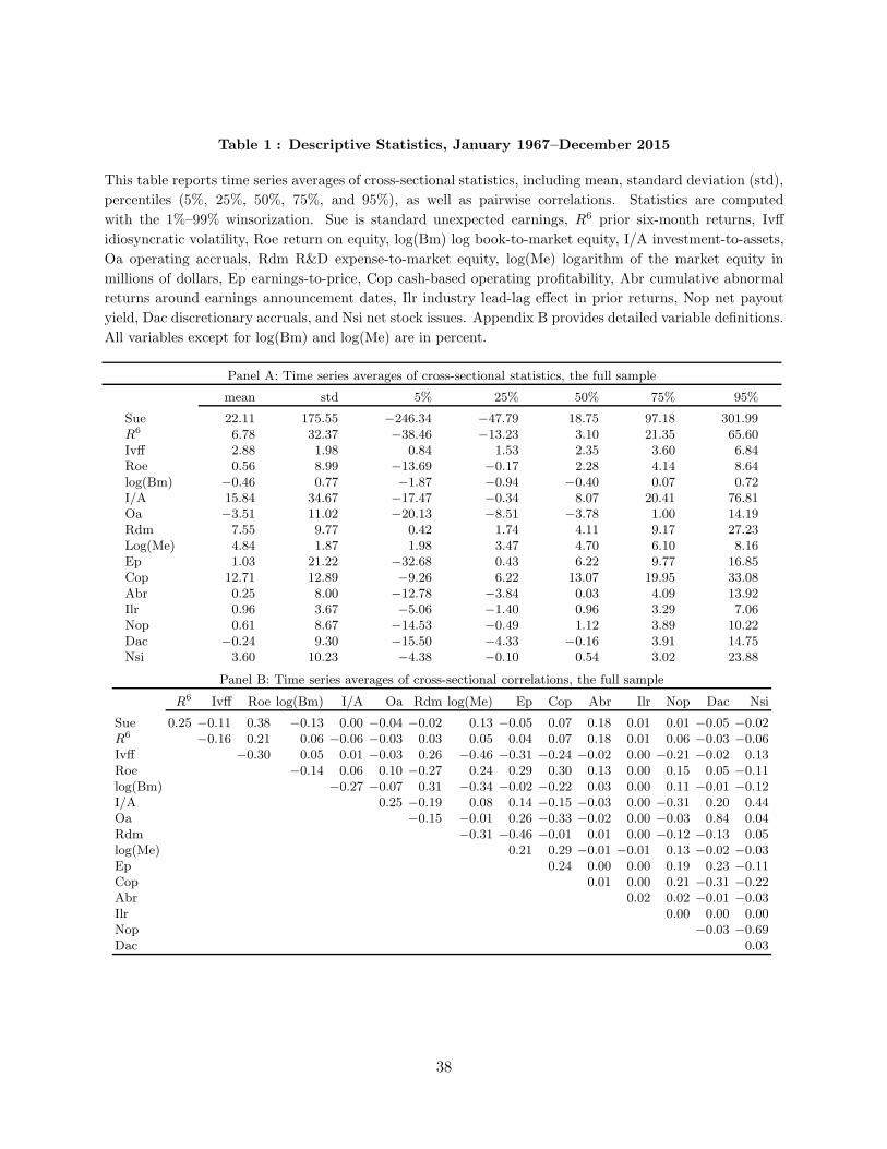
Table 1 : Descriptive Statistics, January 1967–December 2015

This table reports time series averages of cross-sectional statistics, including mean, standard deviation (std),

percentiles (5%, 25%, 50%, 75%, and 95%), as well as pairwise correlations. Statistics are computed

with the 1%–99% winsorization. Sue is standard unexpected earnings, R6 prior six-month returns, Ivff

idiosyncratic volatility, Roe return on equity, log(Bm) log book-to-market equity, I/A investment-to-assets,

Oa operating accruals, Rdm R&D expense-to-market equity, log(Me) logarithm of the market equity in

millions of dollars, Ep earnings-to-price, Cop cash-based operating profitability, Abr cumulative abnormal

returns around earnings announcement dates, Ilr industry lead-lag effect in prior returns, Nop net payout

yield, Dac discretionary accruals, and Nsi net stock issues. Appendix B provides detailed variable definitions.

All variables except for log(Bm) and log(Me) are in percent.

Panel A: Time series averages of cross-sectional statistics, the full sample

mean std 5% 25% 50% 75% 95%

Sue 22.11 175.55 −246.34 −47.79 18.75 97.18 301.99R6 6.78 32.37 −38.46 −13.23 3.10 21.35 65.60Ivff 2.88 1.98 0.84 1.53 2.35 3.60 6.84Roe 0.56 8.99 −13.69 −0.17 2.28 4.14 8.64log(Bm) −0.46 0.77 −1.87 −0.94 −0.40 0.07 0.72I/A 15.84 34.67 −17.47 −0.34 8.07 20.41 76.81Oa −3.51 11.02 −20.13 −8.51 −3.78 1.00 14.19Rdm 7.55 9.77 0.42 1.74 4.11 9.17 27.23Log(Me) 4.84 1.87 1.98 3.47 4.70 6.10 8.16Ep 1.03 21.22 −32.68 0.43 6.22 9.77 16.85Cop 12.71 12.89 −9.26 6.22 13.07 19.95 33.08Abr 0.25 8.00 −12.78 −3.84 0.03 4.09 13.92Ilr 0.96 3.67 −5.06 −1.40 0.96 3.29 7.06Nop 0.61 8.67 −14.53 −0.49 1.12 3.89 10.22Dac −0.24 9.30 −15.50 −4.33 −0.16 3.91 14.75Nsi 3.60 10.23 −4.38 −0.10 0.54 3.02 23.88

Panel B: Time series averages of cross-sectional correlations, the full sample

R6 Ivff Roe log(Bm) I/A Oa Rdm log(Me) Ep Cop Abr Ilr Nop Dac Nsi

Sue 0.25 −0.11 0.38 −0.13 0.00 −0.04 −0.02 0.13 −0.05 0.07 0.18 0.01 0.01 −0.05 −0.02R6 −0.16 0.21 0.06 −0.06 −0.03 0.03 0.05 0.04 0.07 0.18 0.01 0.06 −0.03 −0.06Ivff −0.30 0.05 0.01 −0.03 0.26 −0.46 −0.31 −0.24 −0.02 0.00 −0.21 −0.02 0.13Roe −0.14 0.06 0.10 −0.27 0.24 0.29 0.30 0.13 0.00 0.15 0.05 −0.11log(Bm) −0.27 −0.07 0.31 −0.34 −0.02 −0.22 0.03 0.00 0.11 −0.01 −0.12I/A 0.25 −0.19 0.08 0.14 −0.15 −0.03 0.00 −0.31 0.20 0.44Oa −0.15 −0.01 0.26 −0.33 −0.02 0.00 −0.03 0.84 0.04Rdm −0.31 −0.46 −0.01 0.01 0.00 −0.12 −0.13 0.05log(Me) 0.21 0.29 −0.01 −0.01 0.13 −0.02 −0.03Ep 0.24 0.00 0.00 0.19 0.23 −0.11Cop 0.01 0.00 0.21 −0.31 −0.22Abr 0.02 0.02 −0.01 −0.03Ilr 0.00 0.00 0.00Nop −0.03 −0.69Dac 0.03

38

Panel C: Time series averages of cross-sectional statistics, the all-but-micro sample

mean std 5% 25% 50% 75% 95%

Sue 44.69 185.09 −228.62 −35.27 33.29 126.66 358.08R6 10.58 27.43 −26.09 −6.21 6.95 22.53 59.84Ivff 2.00 1.10 0.79 1.25 1.75 2.46 3.99Roe 2.76 6.07 −4.16 1.55 3.10 4.78 9.28log(Bm) −0.68 0.72 −2.01 −1.12 −0.60 −0.17 0.36I/A 17.97 31.63 −8.15 2.87 9.92 21.36 73.52Oa −3.65 8.99 −16.36 −7.68 −3.91 −0.10 10.04Rdm 4.63 5.61 0.34 1.30 2.87 5.77 14.80Log(Me) 6.48 1.22 4.91 5.52 6.25 7.26 8.86Ep 5.44 10.65 −6.49 3.81 6.73 9.42 14.61Cop 16.35 10.63 0.25 10.15 15.84 22.16 34.78Abr 0.48 6.50 −9.80 −2.91 0.31 3.78 11.24Ilr 0.97 3.69 −5.02 −1.45 0.95 3.35 7.07Nop 1.63 6.57 −8.55 −0.10 1.77 4.33 9.58Dac −0.42 7.47 −12.03 −3.57 −0.29 2.84 10.73Nsi 3.09 9.05 −4.23 −0.36 0.58 2.98 20.10

Panel D: Time series averages of cross-sectional correlations, the all-but-micro sample

R6 Ivff Roe log(Bm) I/A Oa Rdm log(Me) Ep Cop Abr Ilr Nop Dac Nsi

Sue 0.22−0.06 0.41 −0.17 0.03−0.01−0.06 0.06−0.07 0.08 0.15 0.01−0.02−0.03−0.02R6 0.00 0.11 0.04−0.03−0.03 0.09 −0.12−0.03 0.00 0.19 0.01−0.01−0.03−0.02Ivff −0.13 −0.14 0.15 0.00 0.14 −0.31−0.22−0.11 0.00 0.01−0.20−0.02 0.13Roe −0.24 0.05 0.09−0.22 0.11 0.17 0.28 0.08 0.00 0.08 0.04−0.08log(Bm) −0.27−0.07 0.26 −0.11 0.21−0.33 0.01 0.00 0.12 0.02−0.05I/A 0.20−0.12 −0.05 0.00−0.16−0.01 0.00−0.35 0.15 0.48Oa −0.15 −0.06 0.19−0.34−0.01 0.00−0.03 0.82 0.04Rdm −0.12−0.29 0.07 0.02 0.00−0.06−0.15 0.04log(Me) 0.07 0.19−0.05−0.01 0.14−0.03−0.06Ep 0.12−0.01 0.01 0.19 0.19−0.13Cop 0.00 0.01 0.16−0.32−0.22Abr 0.04 0.00−0.01−0.01Ilr 0.00 0.00 0.00Nop −0.02−0.65Dac 0.02

39

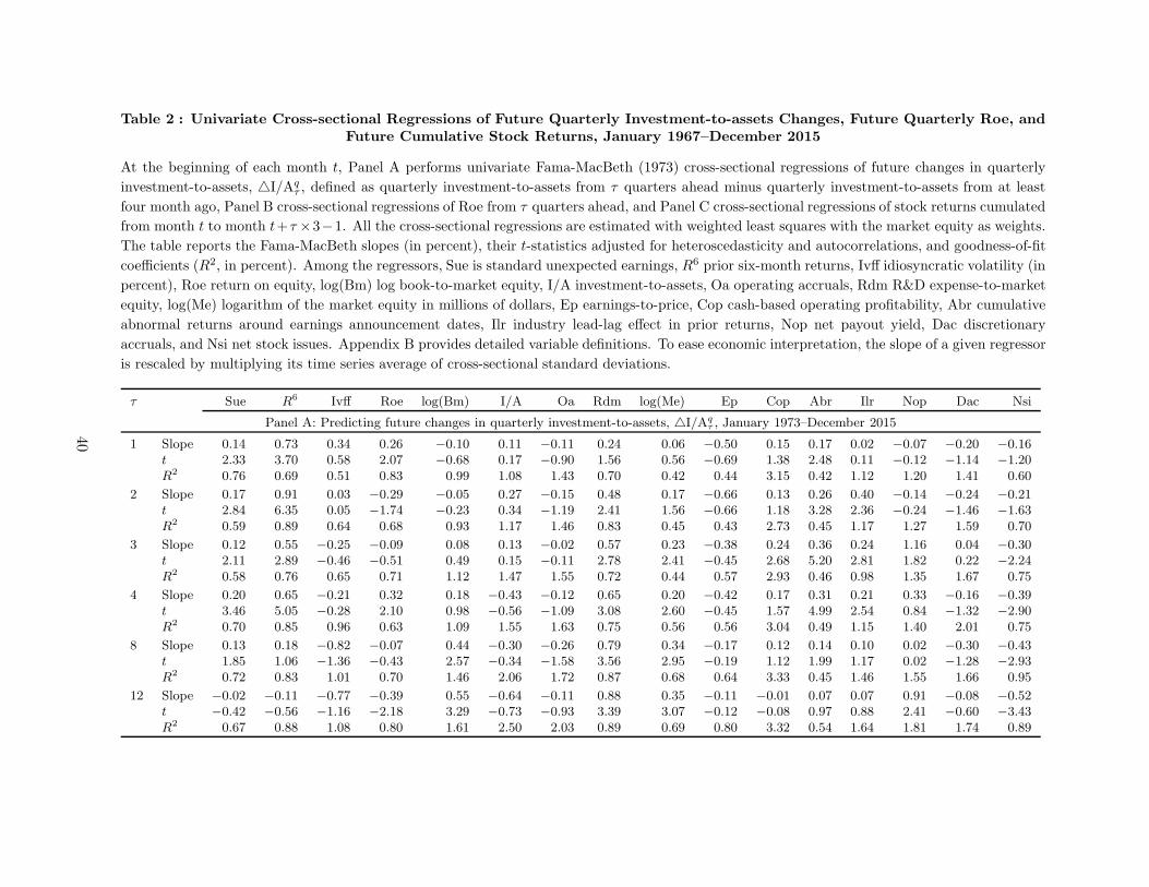
Table 2 : Univariate Cross-sectional Regressions of Future Quarterly Investment-to-assets Changes, Future Quarterly Roe, andFuture Cumulative Stock Returns, January 1967–December 2015

At the beginning of each month t, Panel A performs univariate Fama-MacBeth (1973) cross-sectional regressions of future changes in quarterly

investment-to-assets, △I/Aqτ , defined as quarterly investment-to-assets from τ quarters ahead minus quarterly investment-to-assets from at least

four month ago, Panel B cross-sectional regressions of Roe from τ quarters ahead, and Panel C cross-sectional regressions of stock returns cumulated

from month t to month t+τ ×3−1. All the cross-sectional regressions are estimated with weighted least squares with the market equity as weights.

The table reports the Fama-MacBeth slopes (in percent), their t-statistics adjusted for heteroscedasticity and autocorrelations, and goodness-of-fit

coefficients (R2, in percent). Among the regressors, Sue is standard unexpected earnings, R6 prior six-month returns, Ivff idiosyncratic volatility (in

percent), Roe return on equity, log(Bm) log book-to-market equity, I/A investment-to-assets, Oa operating accruals, Rdm R&D expense-to-market

equity, log(Me) logarithm of the market equity in millions of dollars, Ep earnings-to-price, Cop cash-based operating profitability, Abr cumulative

abnormal returns around earnings announcement dates, Ilr industry lead-lag effect in prior returns, Nop net payout yield, Dac discretionary

accruals, and Nsi net stock issues. Appendix B provides detailed variable definitions. To ease economic interpretation, the slope of a given regressor

is rescaled by multiplying its time series average of cross-sectional standard deviations.

τ Sue R6 Ivff Roe log(Bm) I/A Oa Rdm log(Me) Ep Cop Abr Ilr Nop Dac Nsi

Panel A: Predicting future changes in quarterly investment-to-assets, △I/Aqτ , January 1973–December 2015

1 Slope 0.14 0.73 0.34 0.26 −0.10 0.11 −0.11 0.24 0.06 −0.50 0.15 0.17 0.02 −0.07 −0.20 −0.16t 2.33 3.70 0.58 2.07 −0.68 0.17 −0.90 1.56 0.56 −0.69 1.38 2.48 0.11 −0.12 −1.14 −1.20R2 0.76 0.69 0.51 0.83 0.99 1.08 1.43 0.70 0.42 0.44 3.15 0.42 1.12 1.20 1.41 0.60

2 Slope 0.17 0.91 0.03 −0.29 −0.05 0.27 −0.15 0.48 0.17 −0.66 0.13 0.26 0.40 −0.14 −0.24 −0.21t 2.84 6.35 0.05 −1.74 −0.23 0.34 −1.19 2.41 1.56 −0.66 1.18 3.28 2.36 −0.24 −1.46 −1.63R2 0.59 0.89 0.64 0.68 0.93 1.17 1.46 0.83 0.45 0.43 2.73 0.45 1.17 1.27 1.59 0.70

3 Slope 0.12 0.55 −0.25 −0.09 0.08 0.13 −0.02 0.57 0.23 −0.38 0.24 0.36 0.24 1.16 0.04 −0.30t 2.11 2.89 −0.46 −0.51 0.49 0.15 −0.11 2.78 2.41 −0.45 2.68 5.20 2.81 1.82 0.22 −2.24R2 0.58 0.76 0.65 0.71 1.12 1.47 1.55 0.72 0.44 0.57 2.93 0.46 0.98 1.35 1.67 0.75

4 Slope 0.20 0.65 −0.21 0.32 0.18 −0.43 −0.12 0.65 0.20 −0.42 0.17 0.31 0.21 0.33 −0.16 −0.39t 3.46 5.05 −0.28 2.10 0.98 −0.56 −1.09 3.08 2.60 −0.45 1.57 4.99 2.54 0.84 −1.32 −2.90R2 0.70 0.85 0.96 0.63 1.09 1.55 1.63 0.75 0.56 0.56 3.04 0.49 1.15 1.40 2.01 0.75

8 Slope 0.13 0.18 −0.82 −0.07 0.44 −0.30 −0.26 0.79 0.34 −0.17 0.12 0.14 0.10 0.02 −0.30 −0.43t 1.85 1.06 −1.36 −0.43 2.57 −0.34 −1.58 3.56 2.95 −0.19 1.12 1.99 1.17 0.02 −1.28 −2.93R2 0.72 0.83 1.01 0.70 1.46 2.06 1.72 0.87 0.68 0.64 3.33 0.45 1.46 1.55 1.66 0.95

12 Slope −0.02 −0.11 −0.77 −0.39 0.55 −0.64 −0.11 0.88 0.35 −0.11 −0.01 0.07 0.07 0.91 −0.08 −0.52t −0.42 −0.56 −1.16 −2.18 3.29 −0.73 −0.93 3.39 3.07 −0.12 −0.08 0.97 0.88 2.41 −0.60 −3.43R2 0.67 0.88 1.08 0.80 1.61 2.50 2.03 0.89 0.69 0.80 3.32 0.54 1.64 1.81 1.74 0.89

40

τ Sue R6 Ivff Roe log(Bm) I/A Oa Rdm log(Me) Ep Cop Abr Ilr Nop Dac Nsi

Panel B: Predicting future quarterly Roe, January 1967–December 2015

1 Slope 0.98 1.23 −2.32 5.77 −1.96 0.14 0.51 −2.34 1.47 1.95 1.95 0.48 0.11 1.17 0.01 −0.74t 24.95 13.63 −17.77 71.78 −26.15 1.83 7.95 −12.68 19.64 5.64 26.08 13.47 4.17 8.94 0.29 −11.73R2 8.04 4.07 4.87 36.78 19.21 2.22 1.07 4.57 5.35 4.16 13.31 0.85 1.78 2.31 0.97 1.96

2 Slope 0.93 1.25 −2.37 5.07 −1.88 0.05 0.48 −2.34 1.49 1.87 1.94 0.48 0.19 1.23 0.00 −0.77t 20.23 14.12 −17.64 52.89 −24.51 0.68 7.01 −11.78 19.91 5.36 24.95 12.75 6.68 8.92 0.01 −11.80R2 6.97 4.26 5.02 28.22 18.20 2.04 1.10 4.45 5.64 3.96 13.27 0.88 1.98 2.46 1.06 2.09

3 Slope 0.91 1.25 −2.49 5.00 −1.83 0.11 0.44 −2.36 1.55 1.79 1.92 0.40 0.21 1.27 0.00 −0.80t 20.59 12.38 −15.16 55.67 −23.55 0.85 6.42 −10.30 17.71 4.95 22.71 10.37 5.30 9.02 −0.08 −11.78R2 6.69 3.95 4.85 26.23 16.79 1.86 0.97 4.17 5.64 3.79 12.48 0.69 2.00 2.37 1.02 2.01

4 Slope 0.98 1.21 −2.43 5.88 −1.75 −0.03 0.38 −2.28 1.49 1.51 1.83 0.56 0.19 1.33 −0.05 −0.78t 23.89 12.08 −16.52 59.31 −23.96 −0.49 5.92 −11.65 19.97 4.36 26.89 11.78 6.06 8.54 −1.11 −12.01R2 8.04 3.84 4.72 37.28 16.01 1.59 0.87 4.47 5.61 3.64 12.08 0.95 2.03 2.63 0.97 2.02

8 Slope 0.84 0.83 −2.35 4.99 −1.59 −0.17 0.22 −2.30 1.49 0.94 1.66 0.32 0.12 1.25 −0.20 −0.79t 21.27 10.30 −18.10 47.51 −21.68 −3.38 4.02 −9.18 20.39 3.23 28.18 7.43 3.99 9.82 −4.58 −15.04R2 5.88 2.61 4.31 24.63 12.88 1.08 0.73 4.43 5.47 3.34 10.32 0.75 1.83 2.20 1.09 1.89

12 Slope 0.74 0.58 −2.28 4.32 −1.50 −0.28 0.20 −2.28 1.46 0.66 1.54 0.32 0.12 1.28 −0.20 −0.79t 18.03 7.38 −18.66 39.37 −21.63 −4.54 4.63 −8.37 20.03 2.70 26.23 6.86 3.41 10.76 −5.25 −15.94R2 4.59 1.89 3.91 17.84 10.88 1.16 0.61 4.16 5.25 2.58 9.50 0.69 1.84 2.11 1.03 1.75

Panel C: Predicting future cumulative stock returns from month t to month t+ τ × 3− 1, January 1967–December 2015

1 Slope 0.28 0.59 −0.64 0.47 0.34 −0.59 −0.31 1.00 −0.33 1.25 0.32 0.33 0.23 0.68 −0.36 −0.51t 3.20 2.03 −1.51 1.41 1.92 −2.98 −2.00 2.50 −1.45 1.84 1.98 2.85 2.16 2.50 −2.53 −4.39R2 1.48 3.22 3.88 1.70 3.59 1.73 1.19 2.36 3.54 2.01 2.19 0.69 2.92 1.51 1.15 0.89

2 Slope 0.43 1.80 −1.08 0.70 0.78 −1.18 −0.70 1.94 −0.62 2.35 0.59 0.73 0.28 1.37 −0.72 −1.01t 3.05 3.52 −1.50 1.29 2.59 −3.60 −2.65 2.93 −1.58 2.04 2.05 3.94 1.77 2.98 −2.83 −5.24R2 1.35 3.40 3.82 1.75 3.88 1.74 1.21 2.48 3.67 2.19 2.43 0.62 2.96 1.69 1.23 1.03

3 Slope 0.46 2.70 −1.18 0.46 1.19 −1.65 −1.09 2.74 −0.89 3.16 0.91 1.01 0.51 2.02 −1.05 −1.48t 2.48 4.12 −1.28 0.66 3.04 −4.05 −3.33 3.19 −1.68 2.13 2.32 3.98 2.56 3.43 −3.19 −5.95R2 1.31 3.55 3.68 1.80 4.22 1.66 1.16 2.41 3.75 2.44 2.67 0.64 3.09 1.72 1.24 1.10

4 Slope 0.42 2.76 −1.32 0.20 1.59 −2.06 −1.36 3.63 −1.20 3.80 1.18 1.18 0.89 2.53 −1.33 −1.91t 1.82 3.55 −1.20 0.22 3.33 −4.17 −3.60 3.41 −1.84 2.20 2.42 3.74 3.47 3.61 −3.46 −6.50R2 1.28 3.23 3.53 1.84 4.41 1.67 1.11 2.51 3.67 2.46 2.77 0.67 3.05 1.72 1.17 1.13

8 Slope 0.40 1.66 −0.23 −1.32 2.85 −3.60 −1.97 5.25 −2.37 6.56 2.00 1.68 0.62 5.33 −2.62 −3.65t 1.08 1.52 −0.13 −0.81 3.25 −3.74 −3.50 3.36 −2.12 2.42 2.14 3.06 1.64 4.89 −3.96 −8.24R2 1.23 2.31 2.99 1.77 5.07 1.75 1.05 2.47 3.96 2.42 3.04 0.66 2.88 1.80 1.07 1.16

12 Slope 0.14 1.75 1.10 −3.32 3.75 −3.99 −1.96 6.81 −3.48 11.35 2.98 1.62 0.09 8.02 −3.94 −5.93t 0.25 1.32 0.47 −1.42 2.84 −2.74 −2.85 3.71 −2.17 3.15 2.17 2.40 0.18 5.20 −4.46 −10.38R2 1.28 1.97 2.32 1.65 5.35 1.61 0.79 2.11 4.01 2.53 3.01 0.57 2.60 1.89 0.87 1.06

41

Table 3 : Univariate Cross-sectional Regressions of Future Quarterly Investment-to-assets Changes, Future Quarterly Roe, andFuture Cumulative Stock Returns, the All-but-micro Sample, January 1967–December 2015

At the beginning of each month t, Panel A performs univariate Fama-MacBeth (1973) cross-sectional regressions of future changes in quarterly

investment-to-assets, △I/Aqτ , defined as quarterly investment-to-assets from τ quarters ahead minus quarterly investment-to-assets from at least

four month ago, Panel B cross-sectional regressions of Roe from τ quarters ahead, and Panel C cross-sectional regressions of stock returns cumulated

from month t to month t+ τ × 3− 1. Cross-sectional regressions are estimated with ordinary least squares. The table reports the Fama-MacBeth

slopes (in percent), their t-statistics adjusted for heteroscedasticity and autocorrelations, and goodness-of-fit coefficients (R2, in percent). Among

the regressors, Sue is standard unexpected earnings, R6 prior six-month returns, Ivff idiosyncratic volatility (in percent), Roe return on equity,

log(Bm) log book-to-market equity, I/A investment-to-assets, Oa operating accruals, Rdm R&D expense-to-market equity, log(Me) logarithm of

the market equity in millions of dollars, Ep earnings-to-price, Cop cash-based operating profitability, Abr cumulative abnormal returns around

earnings announcement dates, Ilr industry lead-lag effect in prior returns, Nop net payout yield, Dac discretionary accruals, and Nsi net stock

issues. Appendix B provides detailed variable definitions. To ease economic interpretation, the slope of a given regressor is rescaled by multiplying

its time series average of cross-sectional standard deviations.

τ Sue R6 Ivff Roe log(Bm) I/A Oa Rdm log(Me) Ep Cop Abr Ilr Nop Dac Nsi

Panel A: Predicting future changes in quarterly investment-to-assets, △I/Aqτ , January 1973–December 2015

1 Slope 0.17 0.67 0.00 −0.01 0.00 −0.19 −0.15 0.28 −0.22 −0.15 0.12 0.16 −0.05 0.24 −0.06 −0.10t 4.98 3.56 0.02 −0.12 0.00 −0.79 −1.28 4.55 −1.91 −0.52 1.04 5.28 −0.43 1.52 −1.01 −0.73R2 0.27 0.71 0.32 0.48 0.35 0.74 1.34 0.27 0.19 0.24 3.74 0.15 0.37 0.50 0.68 0.39

2 Slope 0.10 0.97 0.07 −0.63 0.11 −0.12 −0.15 0.41 −0.21 −0.37 0.15 0.31 0.21 0.06 −0.15 −0.23t 2.59 5.89 0.29 −6.78 0.50 −0.30 −2.62 4.98 −2.20 −1.01 1.34 7.89 3.21 0.44 −2.42 −2.01R2 0.21 1.09 0.49 0.66 0.48 0.83 0.70 0.36 0.23 0.30 3.56 0.22 0.39 0.54 0.85 0.44

3 Slope 0.09 0.63 −0.26 −0.35 0.34 −0.21 −0.09 0.43 −0.05 −0.31 0.17 0.35 0.24 0.59 −0.05 −0.39t 2.32 3.64 −1.36 −4.11 1.68 −0.48 −1.20 4.48 −0.63 −0.87 2.49 9.71 3.12 2.28 −0.57 −3.78R2 0.23 0.76 0.60 0.55 0.66 1.07 0.64 0.40 0.25 0.37 3.62 0.24 0.39 0.58 0.77 0.51

4 Slope 0.09 0.56 −0.09 −0.02 0.32 −0.77 −0.15 0.42 0.04 −0.53 0.17 0.26 0.23 0.41 −0.14 −0.53t 2.80 4.61 −0.21 −0.32 0.94 −1.87 −3.17 4.66 0.46 −0.91 1.78 8.01 4.06 6.29 −2.90 −4.15R2 0.23 0.61 0.71 0.43 0.91 1.22 0.56 0.41 0.26 0.45 3.82 0.23 0.47 0.61 1.05 0.54

8 Slope −0.05 0.12 −0.74 −0.20 0.88 −0.74 −0.22 0.43 0.24 −0.13 0.29 0.18 0.09 0.62 −0.22 −0.72t −1.45 0.87 −3.31 −2.67 3.99 −1.76 −3.95 5.18 2.53 −0.34 3.09 5.68 1.19 4.84 −4.11 −6.58R2 0.23 0.47 0.91 0.47 1.31 1.71 0.68 0.51 0.34 0.49 3.86 0.16 0.52 0.83 0.86 0.75

12 Slope −0.24 −0.17 −0.78 −0.43 1.02 −0.86 −0.33 0.47 0.30 −0.13 0.15 0.07 0.09 0.77 −0.25 −0.77t −7.34 −1.03 −3.27 −5.05 4.44 −2.05 −3.54 5.45 2.99 −0.31 1.72 2.23 1.17 8.59 −4.77 −6.76R2 0.24 0.55 1.04 0.56 1.55 1.87 2.13 0.54 0.42 0.54 3.95 0.16 0.65 0.96 0.80 0.78

42

τ Sue R6 Ivff Roe log(Bm) I/A Oa Rdm log(Me) Ep Cop Abr Ilr Nop Dac Nsi

Panel B: Predicting future quarterly Roe, January 1967–December 2015

1 Slope 1.18 0.81 −0.99 3.73 −1.01 0.08 0.49 −1.84 0.70 1.39 1.46 0.46 0.04 0.77 0.28 −0.61t 33.39 14.62 −15.75 76.16 −19.96 1.46 11.87 −12.82 14.75 10.42 25.49 22.27 1.97 10.43 7.16 −10.73R2 6.04 3.59 3.16 32.75 8.02 1.61 1.05 5.30 1.48 4.21 7.30 0.85 0.68 1.79 0.62 1.55

2 Slope 1.06 0.81 −1.02 3.07 −0.93 −0.01 0.46 −1.80 0.72 1.35 1.42 0.39 0.13 0.80 0.25 −0.63t 28.44 16.56 −15.81 48.03 −17.22 −0.21 8.03 −11.65 15.36 9.75 25.56 21.26 6.07 10.14 6.10 −10.91R2 4.97 3.53 3.24 21.87 7.08 1.39 0.99 4.98 1.60 3.95 7.15 0.71 0.78 1.84 0.72 1.59

3 Slope 0.94 0.91 −1.11 3.00 −0.87 0.02 0.41 −0.77 0.74 1.32 1.42 0.33 0.06 0.80 0.25 −0.68t 15.03 7.10 −14.54 56.51 −14.43 0.15 7.97 −0.83 13.97 9.45 21.37 9.30 0.71 10.56 5.72 −11.31R2 4.32 3.24 3.27 20.38 6.07 1.33 0.78 4.60 1.69 3.43 6.53 0.59 0.87 1.82 0.57 1.61

4 Slope 0.96 0.78 −1.08 3.62 −0.79 −0.14 0.52 −1.73 0.74 1.19 1.26 0.46 0.05 0.83 0.24 −0.74t 7.04 15.06 −15.86 54.19 −14.12 −2.78 2.96 −11.58 15.96 9.15 12.60 17.06 0.63 10.77 4.54 −8.19R2 5.56 3.05 3.33 30.21 5.57 1.23 0.85 4.85 1.81 3.11 6.45 1.05 0.94 1.95 0.66 1.87

8 Slope 0.89 0.44 −1.14 2.93 −0.64 −0.31 0.27 −1.59 0.84 1.06 1.28 0.33 0.07 0.91 0.14 −0.76t 25.58 8.78 −16.80 47.72 −11.13 −7.18 5.29 −10.93 17.05 9.34 25.83 11.18 2.79 12.96 4.36 −14.72R2 3.22 1.63 3.20 17.40 3.59 1.05 0.59 3.54 1.96 2.40 5.34 0.58 0.66 1.93 0.50 1.82

12 Slope 0.72 0.29 −1.09 2.44 −0.55 −0.43 0.19 −1.42 0.84 0.93 1.20 0.20 0.06 0.83 0.52 −0.64t 24.03 5.87 −18.21 40.39 −11.85 −5.18 4.13 −10.10 17.11 8.74 20.15 7.17 2.33 12.88 1.23 −7.02R2 2.05 1.17 2.70 11.38 2.74 1.04 0.44 3.02 1.87 1.73 4.71 0.31 0.67 1.51 0.59 1.52

Panel C: Predicting future cumulative stock returns from month t to month t+ τ × 3− 1, January 1967–December 2015

1 Slope 0.53 0.72 −0.58 0.79 0.49 −0.59 −0.25 0.64 −0.29 0.58 0.47 0.50 0.50 0.33 −0.25 −0.60t 6.12 3.60 −2.86 4.61 2.82 −4.41 −2.70 3.09 −2.02 2.25 4.75 7.54 4.80 2.50 −3.61 −6.73R2 0.76 2.19 2.85 1.11 2.14 1.22 0.70 1.29 1.62 1.33 0.81 0.37 1.49 0.98 0.40 0.77

2 Slope 0.76 1.64 −1.07 1.30 1.06 −1.18 −0.50 1.10 −0.49 1.28 0.89 0.83 0.67 0.68 −0.45 −1.21t 5.32 4.61 −3.09 4.45 3.69 −5.34 −3.30 3.36 −2.05 3.01 5.10 8.11 4.10 3.14 −3.77 −8.35R2 0.75 2.39 2.85 1.14 2.36 1.24 0.73 1.24 1.63 1.53 0.96 0.35 1.53 1.06 0.44 0.90

3 Slope 0.81 2.30 −1.49 1.27 1.58 −1.69 −0.81 1.46 −0.65 1.87 1.37 1.12 0.93 1.07 −0.71 −1.80t 4.46 4.87 −3.40 3.37 4.32 −5.92 −4.21 3.39 −2.02 3.28 5.60 7.96 4.76 3.75 −4.40 −9.89R2 0.67 2.61 2.85 1.12 2.52 1.32 0.72 1.23 1.63 1.65 1.12 0.36 1.61 1.11 0.48 1.00

4 Slope 0.81 2.38 −1.82 1.21 2.02 −2.14 −1.08 1.88 −0.77 2.29 1.82 1.23 1.31 1.40 −0.97 −2.33t 3.90 4.27 −3.52 2.56 4.55 −6.07 −4.76 3.61 −1.94 3.27 5.99 7.09 5.36 4.02 −4.90 −10.70R2 0.56 2.38 2.82 1.05 2.54 1.33 0.72 1.34 1.63 1.65 1.20 0.35 1.62 1.14 0.49 1.05

8 Slope 1.07 1.69 −2.72 1.23 3.70 −3.85 −2.04 3.08 −1.08 3.82 3.38 1.65 1.05 3.12 −2.04 −4.57t 3.44 2.23 −3.16 1.61 4.73 −6.13 −5.73 3.70 −1.75 3.33 6.00 5.77 2.80 5.68 −5.68 −14.13R2 0.47 1.58 2.40 0.85 2.61 1.25 0.75 1.45 1.64 1.35 1.38 0.29 1.47 1.18 0.56 1.07

12 Slope 0.86 1.79 −3.26 0.16 5.40 −4.59 −3.01 5.60 −1.98 6.31 5.03 1.74 0.77 4.38 −3.30 −6.31t 1.64 1.94 −2.74 0.14 5.24 −4.48 −5.92 4.67 −2.14 5.39 6.19 4.66 1.67 5.71 −6.31 −11.94R2 0.52 1.33 2.02 0.81 2.56 1.31 0.74 1.43 1.68 1.16 1.56 0.26 1.31 1.19 0.53 1.02

43

Table 4 : Multiple Cross-sectional Regressions of Future Quarterly Investment-to-assets Changes, July 1976–December 2015

At the beginning of each month t, we perform multiple Fama-MacBeth (1973) cross-sectional regressions of future changes in quarterly investment-

to-assets,△I/Aqτ , defined as quarterly investment-to-assets from τ quarters ahead minus quarterly investment-to-assets from at least four month ago.

The cross-sectional regressions are estimated with weighted least squares with the market equity as weights in the full sample in Panel A, and with

ordinary least squares in the all-but-micro sample in Panel B. We report the slopes (in percent), their t-statistics adjusted for heteroscedasticity and

autocorrelations, and goodness-of-fit coefficients (R2, in percent). Among the regressors, Sue is standard unexpected earnings, R6 prior six-month

returns, Ivff idiosyncratic volatility (in percent), Roe return on equity, log(Bm) log book-to-market equity, I/A investment-to-assets, Oa operating

accruals, Rdm R&D expense-to-market equity, log(Me) logarithm of the market equity in millions of dollars, Ep earnings-to-price, Cop cash-based

operating profitability, Abr cumulative abnormal returns around earnings announcement dates, Ilr industry lead-lag effect in prior returns, Nop

net payout yield, Dac discretionary accruals, and Nsi net stock issues. Appendix B provides detailed variable definitions. Multiple regressions use

all these variables simultaneously. The slope of a given regressor is rescaled by multiplying its average cross-sectional standard deviation.

τ Sue R6 Ivff Roe log(Bm) I/A Oa Rdm log(Me) Ep Cop Abr Ilr Nop Dac Nsi R2

Panel A: The full sample, weighted least squares

1 Slope 0.05 0.80 −0.03 0.96 0.17 −0.46 −0.14 0.04 −0.10 −0.03 −0.10 −0.02 −0.17 −0.01 −0.02 −0.02 13.40t 0.58 6.90 −0.26 4.17 1.25 −3.59 −0.61 0.23 −1.26 −0.18 −0.82 −0.15 −2.47 −0.10 −0.09 −0.14

2 Slope 0.28 0.97 −0.17 −0.50 −0.08 −0.58 −0.06 0.04 −0.04 0.27 −0.03 0.16 0.07 0.08 −0.07 −0.03 13.19t 3.01 7.88 −1.18 −2.24 −0.50 −4.25 −0.25 0.17 −0.36 1.26 −0.18 1.73 1.05 0.58 −0.30 −0.20

3 Slope 0.23 0.52 −0.38 −0.39 0.00 −0.64 −0.14 0.05 −0.04 −0.09 0.01 0.35 0.14 0.03 0.04 −0.10 13.25t 2.75 4.51 −2.65 −1.70 0.01 −4.71 −0.61 0.26 −0.41 −0.43 0.08 4.29 2.03 0.23 0.18 −0.62

4 Slope 0.22 0.35 −0.49 0.35 0.29 −0.73 −0.32 0.16 −0.03 −0.71 0.02 0.22 −0.07 −0.08 0.13 −0.26 13.71t 2.71 2.66 −3.64 1.76 1.91 −5.79 −1.55 0.71 −0.27 −2.99 0.11 2.52 −1.09 −0.55 0.74 −1.81

8 Slope 0.29 0.28 −0.56 −0.12 0.63 −0.93 0.09 −0.07 0.17 −1.21 0.31 −0.02 −0.03 0.23 0.09 −0.18 15.58t 2.87 2.30 −3.59 −0.55 3.83 −6.40 0.37 −0.33 1.47 −5.43 2.12 −0.22 −0.44 1.50 0.40 −1.20

12 Slope 0.07 0.19 −0.51 −0.14 0.60 −1.08 −0.14 0.19 0.26 −1.32 0.22 −0.01 −0.03 0.72 0.25 −0.06 15.58t 1.02 1.39 −3.24 −0.64 3.11 −6.85 −0.56 0.86 1.78 −4.04 1.23 −0.07 −0.28 4.19 1.15 −0.37

Panel B: The all-but-micro sample, ordinary least squares

1 Slope 0.03 0.71 −0.03 0.40 0.07 −0.27 −0.02 0.08 −0.04 −0.04 −0.07 0.06 −0.04 −0.04 −0.07 0.00 6.73t 0.58 10.23 −0.67 3.81 0.73 −3.30 −0.15 1.20 −1.00 −0.53 −0.98 1.37 −1.16 −0.53 −0.83 −0.02

2 Slope 0.23 1.02 −0.15 −0.72 0.06 −0.28 0.04 −0.01 −0.01 −0.01 0.12 0.18 0.09 −0.02 −0.04 −0.08 7.06t 4.29 14.58 −2.80 −6.19 0.57 −3.22 0.31 −0.10 −0.31 −0.09 1.47 3.83 2.39 −0.29 −0.40 −0.86

3 Slope 0.18 0.74 −0.21 −0.53 0.29 −0.37 0.09 0.03 0.05 −0.16 0.22 0.29 0.20 −0.03 −0.05 −0.10 7.33t 3.38 10.36 −3.36 −4.65 2.49 −4.13 0.70 0.37 0.91 −1.90 2.38 7.26 5.08 −0.31 −0.54 −1.01

4 Slope 0.09 0.59 −0.35 −0.09 0.49 −0.40 −0.08 0.08 0.03 −0.34 0.19 0.20 0.13 −0.07 0.05 −0.22 7.17t 1.82 8.90 −6.51 −1.11 4.13 −4.48 −0.65 1.14 0.55 −3.88 2.11 4.72 3.29 −0.91 0.49 −2.43

8 Slope 0.04 0.18 −0.44 −0.35 0.87 −0.49 −0.07 −0.03 0.14 −0.44 0.41 0.14 0.00 0.06 0.14 −0.34 8.06t 0.81 2.38 −7.85 −3.48 6.48 −5.88 −0.50 −0.39 2.76 −4.97 4.34 3.63 0.08 0.73 1.22 −3.87

12 Slope −0.14 0.03 −0.47 −0.45 0.91 −0.46 −0.26 0.03 0.21 −0.30 0.31 0.11 0.00 0.14 0.25 −0.38 8.83t −2.61 0.36 −7.46 −4.08 6.30 −4.46 −1.87 0.37 3.60 −3.24 3.10 2.53 0.06 1.70 2.14 −4.24

44

Table 5 : Deciles Formed on Expected Changes in Quarterly Investment-to-assets, July1976–December 2015

Panel A uses all 16 predictors described in Table 1 to form expected changes in quarterly investment-to-

assets, Et[△I/Aq

τ ], with the forecasting horizon, τ , ranging from 1 to 12 quarters. At the beginning of each

month t, we calculate Et[△I/Aq

τ ] with the latest predictor values known and the average cross-sectional

regression slopes estimated with the data from month t − 120− τ × 3 to month t − 1 − τ × 3. We require

a minimum of 36 months. Cross-sectional regressions are estimated with weighted least squares with the

market equity as weights. With the calculated Et[△I/Aq

τ ] values at the beginning of month t, we sort all

stocks into deciles based on NYSE breakpoints, and compute value-weighted decile returns for month t. The

deciles are rebalanced at the beginning of month t+1. For each decile and the high-minus-low decile (H−L),

we report the average excess return, m, its t-value, tm, the q-factor alpha, αq, and its t-statistic, tq. The

t-values are adjusted for heteroscedasticity and autocorrelations. In Panel B, we only use anomaly variables

that are significant in univariate cross-sectional regressions of △I/Aq

τ for each τ horizon to form Et[△I/Aq

τ ].

For τ = 1, the set of significant predictors includes Sue, R6, Roe, and Abr; for τ = 2, Sue, R6, Rdm, Abr,

and Ilr; for τ = 3, Sue, R6, Rdm, log(Me), Cop, Abr, Ilr, and Nsi; for τ = 4, Sue, R6, Roe, Rdm, log(Me),

Abr, Ilr, and Nsi; for τ = 8, log(Bm), Rdm, log(Me), and Nsi; and for τ = 12, Roe, log(Bm), Rdm, log(Me),

Nop, and Nsi. All other aspects of the test design in Panel B are identical to those in Panel A.

Panel A: Using all 16 anomaly variables to form expected changes in quarterly I/A

τ Low 2 3 4 5 6 7 8 9 High H−L

1 m 0.66 0.59 0.56 0.68 0.74 0.92 0.56 0.65 0.56 1.00 0.35tm 1.95 2.13 2.25 2.63 3.06 3.86 2.27 2.60 2.09 3.14 1.19αq 0.61 0.35 0.08 0.12 0.16 0.41 −0.14 −0.03 −0.20 0.31 −0.30tq 2.88 2.27 0.56 0.84 1.24 3.02 −1.14 −0.22 −1.33 1.51 −0.87

2 m 0.73 0.64 0.81 0.54 0.83 0.75 0.79 0.58 0.79 0.83 0.10tm 2.12 2.18 2.80 1.91 3.42 3.19 3.18 2.46 3.02 2.83 0.40αq 0.46 0.31 0.34 0.14 0.11 −0.10 0.05 −0.36 −0.03 0.24 −0.22tq 2.59 1.70 2.02 0.80 0.73 −0.87 0.31 −2.45 −0.19 1.06 −0.69

3 m 0.57 0.74 0.80 0.87 0.86 0.49 0.73 0.73 0.70 0.60 0.03tm 1.61 2.54 2.74 3.20 3.41 1.98 3.14 3.10 2.78 2.11 0.12αq 0.30 0.39 0.55 0.34 0.13 −0.23 −0.14 −0.14 −0.06 −0.03 −0.33tq 1.80 2.27 3.37 2.46 0.96 −1.59 −1.10 −0.97 −0.38 −0.16 −1.28

4 m 0.56 0.63 0.82 0.82 0.87 0.63 0.65 0.75 0.88 0.93 0.37tm 1.65 2.02 2.96 3.11 3.61 2.45 2.86 3.00 3.48 3.22 1.43αq 0.27 0.30 0.42 0.38 0.21 −0.15 −0.10 0.01 0.00 0.30 0.02tq 1.71 1.67 2.75 2.71 1.25 −1.02 −0.73 0.05 0.01 1.44 0.08

8 m 0.61 0.52 0.72 0.78 0.88 0.95 0.80 0.73 0.64 0.81 0.20tm 1.73 1.59 2.36 2.83 3.53 3.83 3.17 3.14 2.47 3.05 0.77αq 0.42 0.23 0.27 0.23 0.22 0.23 0.01 0.04 −0.08 0.23 −0.19tq 2.34 1.30 1.41 1.44 1.61 1.84 0.05 0.31 −0.42 1.41 −0.79

12 m 0.78 0.86 0.85 0.74 0.84 0.92 0.71 0.79 0.78 0.91 0.13tm 2.15 2.64 2.83 2.64 3.47 3.57 2.78 3.25 2.96 3.56 0.42αq 0.54 0.27 0.26 0.12 0.20 0.19 −0.06 −0.04 0.15 0.42 −0.12tq 2.83 1.42 1.77 0.79 1.61 1.24 −0.39 −0.31 0.97 1.95 −0.39

45

Panel B: Using only significant predictors in univariate regressions to form expected changes in quarterly I/A

τ Low 2 3 4 5 6 7 8 9 High H−L

1 m 0.49 0.70 0.68 0.59 0.62 0.65 0.63 0.53 0.59 1.02 0.53tm 1.48 2.67 3.17 2.86 3.03 3.27 3.18 2.50 2.54 3.45 1.81αq 0.25 0.33 0.25 0.03 0.07 −0.02 −0.12 −0.23 −0.23 0.20 −0.06tq 1.12 2.08 1.90 0.30 0.67 −0.19 −1.52 −2.62 −2.14 1.01 −0.14

2 m 0.56 0.78 0.70 0.76 0.83 0.65 0.52 0.65 0.63 1.11 0.54tm 1.62 2.59 2.63 3.09 3.35 2.77 2.19 2.68 2.47 3.40 1.84αq 0.43 0.41 0.22 0.22 0.35 −0.02 −0.34 −0.15 −0.10 0.54 0.11tq 1.58 2.14 1.30 1.71 2.53 −0.16 −3.06 −1.15 −0.70 2.09 0.25

3 m 0.28 0.90 0.78 0.70 0.70 0.64 0.83 0.68 0.54 0.98 0.70tm 0.86 3.14 2.88 2.59 2.76 2.52 3.39 2.83 2.06 3.53 2.93αq 0.04 0.51 0.46 0.27 0.18 0.02 0.26 −0.01 −0.20 0.27 0.23tq 0.21 3.03 3.06 1.79 1.35 0.18 1.74 −0.04 −1.27 1.35 0.76

4 m 0.35 0.78 0.66 0.69 0.93 0.56 0.60 0.81 0.66 0.87 0.51tm 1.08 2.60 2.32 2.63 3.84 2.34 2.27 3.54 2.59 3.15 2.38αq 0.12 0.37 0.34 0.19 0.35 −0.07 0.05 0.14 −0.04 0.39 0.27tq 0.67 2.24 1.75 1.43 2.74 −0.65 0.42 1.04 −0.27 2.20 1.20

8 m 0.38 0.83 0.84 0.62 0.73 0.90 0.86 0.62 0.64 0.86 0.49tm 1.01 2.44 2.89 2.21 2.80 3.35 3.40 2.58 2.80 3.92 1.61αq 0.13 0.52 0.40 −0.18 0.14 0.48 0.28 0.01 −0.06 0.26 0.13tq 0.63 3.02 2.73 −1.07 0.80 2.67 1.71 0.07 −0.51 2.06 0.51

12 m 0.86 0.73 0.66 0.89 0.82 1.02 0.80 0.78 0.88 0.69 −0.17tm 2.49 2.16 2.21 3.18 3.18 3.77 3.14 3.12 3.71 2.96 −0.67αq 0.24 0.22 0.14 0.08 0.08 0.24 0.06 0.14 0.12 0.12 −0.12tq 1.26 1.22 0.85 0.52 0.42 1.24 0.40 0.91 0.90 0.95 −0.49

46

Table 6 : Deciles Formed on Expected Changes in Quarterly Investment-to-assets, theAll-but-micro Sample, July 1976–December 2015

Panel A uses all 16 predictors in Table 1 to form expected changes in quarterly investment-to-assets,

Et[△I/Aq

τ ], with the horizon, τ , ranging from 1 to 12 quarters. At the beginning of each month t, we

calculate Et[△I/Aq

τ ] with the latest predictor values known and the average cross-sectional regression slopes

estimated with the data from month t−120−τ×3 to month t−1−τ×3. We require a minimum of 36 months.

Cross-sectional regressions are estimated with ordinary least squares. With the calculated Et[△I/Aq

τ ] values

at the beginning of month t, we sort all-but-micro stocks into deciles, and compute equal-weighted returns

for month t. The deciles are rebalanced at the beginning of month t+1. For each decile and the high-minus-

low decile (H−L), we report the average excess return, m, its t-value, tm, the q-factor alpha, αq, and its

t-statistic, tq. The t-values are adjusted for heteroscedasticity and autocorrelations. In Panel B, we only use

anomaly variables that are significant in univariate cross-sectional regressions of △I/Aq

τ for each τ to form

Et[△I/Aq

τ ]. For τ = 1, the set of significant predictors includes Sue, R6, Rdm, and Abr; for τ = 2, Sue, R6,

Roe, Oa, Rdm, log(Me), Abr, Ilr, Dac, and Nsi; for τ = 3, Sue, R6, Roe, Rdm, Cop, Abr, Ilr, Nop, and Nsi;

for τ = 4, Sue, R6, Oa, Rdm, Abr, Ilr, Nop, Dac, and Nsi; for τ = 8, Ivff, Roe, log(Bm), Oa, Rdm, log(Me),

Cop, Abr, Nop, Dac, and Nsi; and for τ = 12, Sue, Ivff, Roe, log(Bm), I/A, Oa, Rdm, log(Me), Abr, Nop,

Dac, and Nsi. All other aspects of the test design in Panel B are identical to those in Panel A.

Panel A: Using all 16 anomaly variables to form expected changes in quarterly I/A

τ Low 2 3 4 5 6 7 8 9 High H−L

1 m 0.46 0.72 0.69 0.74 0.75 0.93 0.80 0.83 1.14 1.43 0.96tm 1.15 2.13 2.33 2.69 2.82 3.51 2.97 2.90 3.67 3.78 3.52αq 0.24 0.34 0.17 0.15 0.01 0.22 0.08 0.14 0.48 0.87 0.63tq 1.10 1.57 1.04 1.40 0.09 2.38 0.91 1.28 2.82 3.67 1.64

2 m 0.66 0.95 0.75 0.80 0.96 0.86 0.83 0.85 0.97 1.00 0.35tm 1.66 2.81 2.43 2.74 3.50 3.29 3.07 3.02 3.08 2.69 1.27αq 0.34 0.57 0.19 0.16 0.28 0.11 0.08 0.16 0.32 0.49 0.15tq 1.29 3.02 1.27 1.12 2.30 0.97 0.88 1.22 1.85 2.10 0.34

3 m 0.54 0.82 0.81 0.90 0.74 0.95 0.88 0.84 0.98 1.08 0.53tm 1.36 2.38 2.57 3.13 2.67 3.44 3.26 2.97 3.23 2.94 2.05αq 0.28 0.41 0.36 0.27 0.07 0.19 0.16 0.13 0.32 0.54 0.26tq 1.16 2.21 2.23 2.09 0.59 1.58 1.78 1.05 1.91 2.30 0.65

4 m 0.36 0.86 0.75 0.95 0.84 0.94 0.89 0.91 0.94 1.31 0.95tm 0.88 2.46 2.39 3.34 2.91 3.46 3.35 3.24 3.25 3.70 3.92αq 0.16 0.45 0.34 0.39 0.11 0.17 0.09 0.11 0.16 0.67 0.51tq 0.75 2.74 2.46 2.95 1.08 1.69 0.89 1.10 1.10 3.13 1.57

8 m 0.34 0.85 0.78 0.94 0.93 1.01 0.87 0.90 0.79 0.89 0.55tm 0.83 2.35 2.30 3.13 3.18 3.60 3.16 3.11 2.82 2.83 2.35αq 0.16 0.49 0.40 0.47 0.31 0.36 0.10 0.14 0.03 0.17 0.01tq 0.96 3.52 2.96 4.35 3.40 3.75 1.05 1.49 0.28 1.17 0.06

12 m 0.62 0.96 0.84 0.99 1.16 0.95 1.02 0.97 0.97 0.87 0.25tm 1.51 2.66 2.52 3.19 3.82 3.35 3.60 3.52 3.37 2.63 0.93αq 0.24 0.44 0.33 0.42 0.47 0.24 0.23 0.13 0.15 0.07 −0.17tq 1.36 3.36 3.05 3.60 3.90 2.22 2.07 1.25 1.26 0.43 −0.70

47

Panel B: Using only significant predictors in univariate regressions to form expected changes in quarterly I/A

τ Low 2 3 4 5 6 7 8 9 High H−L

1 m 0.58 0.69 0.72 0.80 0.86 0.80 0.77 0.93 1.18 1.38 0.80tm 1.44 2.09 2.46 2.80 3.11 2.89 2.70 2.97 3.40 3.38 2.52αq 0.49 0.32 0.27 0.26 0.26 0.13 0.10 0.30 0.59 0.90 0.41tq 1.80 1.65 1.63 1.96 3.00 1.25 0.82 1.56 2.64 3.07 0.85

2 m 0.65 0.81 0.85 0.91 0.86 0.88 0.83 0.92 0.94 1.09 0.44tm 1.62 2.35 2.73 3.16 3.09 3.35 2.86 3.06 2.80 2.66 1.45αq 0.34 0.37 0.37 0.29 0.24 0.23 0.23 0.32 0.39 0.72 0.38tq 1.22 1.93 2.41 1.99 2.35 2.52 1.75 1.87 1.62 2.57 0.79

3 m 0.53 0.86 0.82 0.88 0.82 0.89 0.80 0.86 1.01 1.10 0.57tm 1.36 2.64 2.73 3.09 2.99 3.28 2.98 2.87 3.10 2.95 2.14αq 0.14 0.33 0.17 0.32 0.17 0.21 0.10 0.23 0.41 0.67 0.53tq 0.54 1.71 1.19 2.08 1.65 2.22 0.98 1.60 2.45 2.83 1.28

4 m 0.46 0.59 0.89 0.81 0.85 0.85 0.92 0.95 1.13 1.27 0.80tm 1.17 1.73 2.96 2.71 3.12 3.19 3.38 3.28 3.53 3.37 3.34αq 0.11 0.05 0.40 0.20 0.17 0.11 0.18 0.30 0.49 0.80 0.70tq 0.51 0.32 2.65 1.52 1.48 1.09 1.83 2.70 2.50 3.33 1.93

8 m 0.31 0.80 0.84 0.82 0.86 0.96 0.99 0.86 0.80 0.83 0.52tm 0.73 2.07 2.47 2.58 2.99 3.40 3.57 2.96 2.88 2.76 1.92αq 0.18 0.49 0.47 0.38 0.26 0.26 0.29 0.11 0.01 0.08 −0.10tq 1.01 3.29 3.92 3.58 2.69 2.65 3.04 1.00 0.13 0.64 −0.44

12 m 0.57 1.00 0.95 1.02 0.97 1.03 1.11 0.86 0.92 0.90 0.33tm 1.35 2.72 2.67 3.12 3.20 3.54 3.94 3.14 3.22 2.92 1.12αq 0.26 0.50 0.54 0.45 0.37 0.32 0.36 0.03 0.02 0.07 −0.19tq 1.32 3.65 3.32 3.77 3.36 3.21 3.46 0.27 0.19 0.49 −0.74

48

Table 7 : Estimates of Implied Costs of Capital for the Fama-French (2015) Factors

AR, IRR, and Diff (all in annual percent) are the average return, the internal rate of return, and AR minus IRR, respectively. SMB, HML, RMW,

and CMA are the Fama-French (2015) size, value, profitability, and investment factors, respectively. Panel A uses the analysts’ earnings forecasts,

Panel B uses the Hou-van Dijk-Zhang (2012) cross-sectional earnings forecasts, and Panel C uses the Tang-Wu-Zhang (2014) cross-sectional Roe

forecasts in estimating the IRRs. GLS denotes the Gebhardt-Lee-Swaminathan model, Easton the Easton model, CT the Claus-Thomas model,

OJ the Ohlson-Juettner-Nauroth model, and Average the averages across the models. Appendix C describes in detail the estimation methods.

Panel A: IBES earnings forecasts Panel B: Cross-sectional earnings forecasts Panel C: Cross-sectional ROE forecasts(1979–2015) (1967–2015) (1967–2015)

AR IRR Diff AR IRR Diff AR IRR Diff AR IRR Diff AR IRR Diff AR IRR Diff

GLS Easton GLS Easton GLS Easton

SMB 1.75 0.87 0.88 1.87 2.52 −0.65 2.85 1.53 1.32 2.85 5.05 −2.20 3.21 0.08 3.14 3.12 1.15 1.97[t] 0.87 4.56 0.44 0.97 14.63 −0.34 1.38 4.02 0.66 1.42 6.90 −1.17 1.63 0.33 1.62 1.58 4.86 1.00HML 3.26 3.50 −0.23 3.16 3.30 −0.14 3.49 5.55 −2.06 3.41 7.22 −3.81 3.80 5.20 −1.39 4.02 7.61 −3.59[t] 1.48 18.39 −0.11 1.37 7.31 −0.06 1.88 26.60 −1.14 1.81 14.99 −1.96 2.03 31.79 −0.77 2.08 15.88 −1.96RMW 3.75 −1.18 4.93 4.43 −3.29 7.72 3.37 −1.44 4.81 3.89 −3.67 7.57 3.00 −1.36 4.36 3.18 −6.41 9.59[t] 2.59 −8.32 3.49 2.70 −9.42 4.60 2.60 −6.58 3.86 2.60 −10.35 4.79 2.37 −7.94 3.56 2.50 −19.65 6.99CMA 3.34 0.64 2.70 3.46 2.45 1.00 3.59 1.61 1.99 4.28 4.06 0.22 3.37 1.11 2.26 3.32 4.58 −1.26[t] 2.69 4.69 2.26 2.95 7.80 0.94 3.01 9.13 1.72 4.10 11.39 0.20 3.03 5.76 2.08 2.81 10.32 −1.12

CT OJ CT OJ CT OJ

SMB 1.79 1.10 0.69 1.94 0.67 1.27 2.92 2.73 0.19 3.90 3.21 0.69 3.46 −1.13 4.59 3.44 −1.39 4.82[t] 0.89 6.79 0.35 0.97 4.43 0.65 1.41 4.23 0.09 2.00 5.32 0.37 1.75 −3.54 2.35 1.68 −3.79 2.32HML 3.38 0.06 3.32 2.23 0.70 1.53 3.28 3.64 −0.36 2.97 4.72 −1.75 3.25 2.55 0.70 3.15 4.15 −1.00[t] 1.50 0.17 1.46 1.03 3.55 0.70 1.76 15.76 −0.19 1.72 17.96 −1.00 1.88 5.76 0.39 1.63 9.27 −0.51RMW 3.71 0.34 3.37 4.11 −0.03 4.14 3.17 −0.00 3.18 3.31 −1.59 4.90 2.55 0.00 2.54 2.11 −2.05 4.16[t] 2.64 2.20 2.42 3.36 −0.17 3.36 2.94 −0.01 2.95 3.30 −5.72 4.60 2.45 0.02 2.43 2.06 −9.07 3.76CMA 3.31 0.08 3.23 3.03 0.07 2.96 3.26 1.52 1.74 3.72 2.10 1.62 2.81 0.62 2.19 3.06 0.70 2.35[t] 2.71 0.58 2.65 2.59 0.42 2.53 2.82 11.24 1.46 3.07 10.62 1.35 2.55 4.25 1.93 2.53 3.30 1.86

Average Average Average

SMB 1.73 1.72 0.01 2.82 3.23 −0.41 3.20 −0.22 3.42[t] 0.90 10.65 0.01 1.36 5.59 −0.21 1.63 −0.83 1.75HML 3.15 2.03 1.13 3.65 5.30 −1.66 3.77 5.09 −1.32[t] 1.36 8.64 0.50 1.92 24.84 −0.88 2.01 17.26 −0.72RMW 4.47 −1.59 6.06 3.47 −1.85 5.32 3.01 −2.46 5.46[t] 2.76 −9.74 3.76 2.52 −9.41 3.88 2.37 −20.72 4.28CMA 3.26 1.15 2.11 3.69 2.64 1.05 3.32 2.04 1.28[t] 2.72 7.01 1.86 3.19 19.47 0.92 3.02 13.60 1.19

49

Table 8 : Annual Cross-sectional Regressions of Future Book Equity Growth Rates and Operating Profitability, 1963–2015

The sample contains all common stocks on NYSE, Amex, and Nasdaq. We do not exclude financial firms, because these stocks are included in the

construction of the Fama-French (2015) five factors. All the regressions are annual cross-sectional regressions. Ait is total assets for firm i at year

t, △Ait ≡ Ait −Ait−1, Beit is book equity for firm i at year t, △Beit ≡ Beit −Beit−1, and Opit is operating profitability for firm i at year t. Book

equity is measured as in Davis, Fama, and French (2000), and operating profitability is measured as in Fama and French (2015). Variables dated t

are measured at the end of the fiscal year ending in calendar year t. To avoid the excess influence of small firms, we follow Fama and French (2006)

and exclude those with total assets below $5 million or book equity below $2.5 million in year t in Panel A. The cutoffs are $25 million and $12.5

million in Panel B. We winsorize all regression variables at the 1st and 99th percentiles of the cross-sectional distribution each year.

△Beit+τ

Beit+τ−1= γ0 + γ1

△Ait

Ait−1+ ǫt+τ

△Beit+τ

Beit+τ−1= γ0 + γ1

△BeitBeit−1

+ ǫt+τ Opit+τ = γ0 + γ1Opit + ǫt+τ

τ #firms γ0 t(γ0) γ1 t(γ1) R2 γ0 t(γ0) γ1 t(γ1) R2 γ0 t(γ0) γ1 t(γ1) R2

Panel A: Firms with assets ≥ $5 million and book equity ≥ $2.5 million

1 3,106 0.09 14.57 0.22 14.38 0.05 0.09 13.14 0.21 8.64 0.06 0.03 4.85 0.79 43.14 0.542 2,844 0.10 14.57 0.10 7.58 0.01 0.10 14.65 0.10 5.23 0.02 0.06 6.67 0.66 28.82 0.363 2,624 0.10 14.98 0.06 6.25 0.01 0.10 14.91 0.06 4.09 0.01 0.08 8.11 0.58 25.35 0.274 2,429 0.10 16.19 0.05 5.47 0.00 0.10 16.20 0.05 3.73 0.00 0.09 9.47 0.52 22.93 0.225 2,256 0.10 15.03 0.04 3.41 0.00 0.10 16.04 0.03 1.91 0.00 0.10 11.37 0.49 23.35 0.196 2,099 0.10 15.26 0.05 4.57 0.00 0.10 15.01 0.03 2.24 0.00 0.11 13.05 0.45 23.72 0.167 1,955 0.10 15.45 0.04 4.39 0.00 0.10 15.58 0.03 2.69 0.00 0.11 14.39 0.42 21.71 0.158 1,821 0.09 15.36 0.03 3.98 0.00 0.10 15.65 0.01 1.60 0.00 0.12 15.82 0.40 19.09 0.139 1,697 0.09 15.28 0.03 3.45 0.00 0.10 15.42 0.01 1.19 0.00 0.12 15.29 0.39 18.10 0.1210 1,584 0.09 14.57 0.04 4.50 0.00 0.09 14.77 0.02 2.17 0.00 0.13 14.61 0.38 17.48 0.11

Panel B: Firms with assets ≥ $25 million and book equity ≥ $12.5 million

1 2,485 0.08 15.82 0.23 17.75 0.05 0.08 14.10 0.24 10.53 0.07 0.03 7.14 0.82 57.60 0.612 2,278 0.09 15.67 0.13 10.23 0.02 0.09 16.03 0.13 7.10 0.02 0.06 9.13 0.69 35.39 0.423 2,103 0.09 16.53 0.08 7.61 0.01 0.09 16.37 0.08 5.82 0.01 0.08 11.01 0.61 31.96 0.324 1,949 0.09 17.04 0.07 6.70 0.01 0.09 16.96 0.07 4.44 0.01 0.09 13.31 0.56 30.26 0.265 1,812 0.09 16.60 0.05 3.90 0.01 0.09 17.23 0.04 2.87 0.01 0.10 16.00 0.51 31.21 0.226 1,689 0.09 16.57 0.05 5.51 0.00 0.09 16.39 0.04 3.37 0.00 0.11 17.71 0.48 32.30 0.197 1,577 0.09 16.80 0.05 4.84 0.00 0.09 16.90 0.04 3.12 0.00 0.12 19.34 0.45 30.53 0.168 1,473 0.09 16.07 0.03 3.92 0.00 0.09 16.08 0.02 2.58 0.00 0.13 19.90 0.43 26.50 0.159 1,375 0.09 15.84 0.03 3.92 0.00 0.09 16.07 0.02 2.08 0.00 0.13 19.14 0.42 23.14 0.1410 1,286 0.09 14.58 0.05 5.35 0.00 0.09 14.84 0.03 3.01 0.00 0.14 18.07 0.40 22.38 0.13

50

Table 9 : Factor Spanning Tests, The PRRT Factor Model, the q-factor Model, and the Carhart Model, January1967–December 2015

Panel A regresses the PRRT factors on the q-factor model and on the Carhart model. fME, fEP, and fBM are the size, earnings yield, and book-

to-market factors from the PRRT model. m denotes average returns, αq is the q-factor alpha, αC the Carhart alpha, and the betas are factor

loadings. Panel B regresses the Carhart factors and q-factors on the PRRT factor model, consisting of the market factor, fME, fEP, and fBM. αP is

the PRRT alpha, and the betas are factor loadings. The Carhart factors data are from Kennenth French’s Web site, and the q-factors data are from

Hou, Xue, and Zhang (2015). To form the PRRT factors, at the end of June of each year t, we use the median NYSE size to split NYSE, Amex,

and NASDAQ stocks into two groups, small and big. Independently, we split stocks into three earnings yield groups using the NYSE breakpoints

for the low 30%, middle 40%, and high 30% of the ranking values for the fiscal year ending in calendar year t − 1. Also independently, we break

stocks into three book-to-market groups using the NYSE breakpoints for the low 30%, middle 40%, and high 30% of the ranking values for the

fiscal year ending in calendar year t− 1. Taking the intersection of the two size, three earnings yield, and three book-to-market groups, we obtain

18 benchmark portfolios. Monthly value-weighted portfolio returns are calculated from July of year t to June of year t+ 1, and the portfolios are

rebalanced at the June of t+ 1. fME is the difference (small-minus-big), each month, between the simple average of the returns on the nine small

portfolios and that of the nine big portfolios. fEP is the difference (high-minus-low), each month, between the simple average of the returns on

the six high earnings yield portfolios and that of the six low earnings yield portfolios. Finally, fBM is the difference (high-minus-low), each month,

between the simple average of the returns on the six high book-to-market portfolios and that of the six low book-to-market portfolios.

Panel A: Explaining the PRRT factors Panel B: The PRRT four-factor regressions

m αq βMKT βME βI/A βROE R2 m αP βMKT βME βEP βBM R2

fME 0.24 0.09 0.01 0.88 −0.19 −0.09 0.91 SMB 0.21 0.01 −0.02 0.97 −0.07 −0.01 0.921.85 2.11 0.96 44.45 −4.77 −3.17 1.59 0.16 −1.35 41.62 −2.37 −0.38

fEP 0.25 −0.01 −0.12 −0.12 0.40 0.34 0.38 HML 0.34 0.05 0.06 0.06 0.43 0.89 0.821.97 −0.11 −3.61 −1.74 4.60 4.33 2.53 0.84 3.42 2.12 9.22 37.49

fBM 0.16 0.06 −0.07 0.01 0.74 −0.31 0.47 UMD 0.69 0.86 −0.20 −0.02 0.00 −0.41 0.071.43 0.72 −2.59 0.16 12.38 −4.81 3.82 4.82 −2.47 −0.14 0.01 −3.23

αC βMKT βSMB βHML βUMD R2

fME 0.02 0.03 0.93 0.05 −0.02 0.92 rME 0.31 0.03 0.00 1.00 0.08 0.09 0.900.50 2.47 74.18 1.93 −1.14 2.34 0.76 0.14 42.80 2.15 3.96

fEP 0.18 −0.12 −0.25 0.41 0.05 0.46 rI/A 0.41 0.36 −0.06 −0.06 0.10 0.39 0.451.96 −4.83 −4.34 8.17 1.12 4.88 5.72 −3.76 −1.96 1.86 12.93

fBM −0.06 −0.05 0.07 0.70 −0.02 0.71 rROE 0.57 0.61 −0.05 −0.17 0.39 −0.45 0.39−0.93 −2.93 3.47 22.00 −1.21 5.36 7.78 −1.68 −3.75 5.40 −9.04

51

A Derivations

We derive the investment CAPM in equation (6), following Liu, Whited, and Zhang (2009). Let qitbe the Lagrangian multiplier associated with Ait+1 = Iit + (1 − δ)Ait. The optimality conditionswith respect to Iit, Ait+1, and Bit+1 from maximizing equation (??) are, respectively,

qit = 1 + (1− τ)∂Φ(Iit, Ait)

∂Iit(A1)

qit = Et

[

Mt+1

[

(1− τ)

[

Xit+1 −∂Φ(Iit+1, Ait+1)

∂Ait+1

]

+ τδ + (1− δ)qit+1

]]

(A2)

1 = Et

[

Mt+1

[

rBit+1 − (rBit+1 − 1)τ t+1

]]

. (A3)

Dividing both sides of equation (A2) by qit and substituting equation (A1), we obtainEt[Mt+1r

Iit+1] = 1, in which rIit+1 is the investment return given by equation (4), after substi-

tuting Φ(Iit, Ait) = (a/2)(Iit/Ait)2Ait.

Equation (A3) says that Et[Mt+1rBit+1] = 1 + Et[Mt+1(r

Bit+1 − 1)τ ]. Intuitively, because of the

tax benefit of debt, the unit price of the pre-tax bond return, Et[Mt+1rBit+1], is higher than one.

The difference is precisely the present value of the tax benefit. Because we define the after-taxcorporate bond return, rBa

it+1 ≡ rBit+1 − (rBit+1 − 1)τ , equation (A3) says that the unit price of theafter-tax corporate bond return is one: Et[Mt+1r

Bait+1] = 1.

To prove equation (5), we first show that qitAit+1 = Pit+Bit+1 under constant returns to scale.We start with Pit +Dit = Vit and expand Vit using equations (3) and (??):

Pit + (1− τ)[Π(Xit, Ait)− Φ(Iit, Ait)− rBitBit]− τBit − Iit +Bit+1 + τδAit =

(1− τ)

[

Π(Xit, Ait)−∂Φ(Iit, Ait)

∂IitIit −

∂Φ(Iit, Ait)

∂AitAit − rBitBit

]

− τBit − Iit +Bit+1 + τδAit

− qit(Ait+1 − (1− δ)Ait − Iit) + Et[Mt+1((1− τ t)

[

Π(Xit+1, Ait+1)−∂Φ(Iit+1, Ait+1)

∂Iit+1Iit+1

−∂Φ(Iit+1, Ait+1)

∂Ait+1Ait+1 − rBit+1Bit+1

]

− τBit+1 − Iit+1 +Bit+2

+ τδAit+1 − qit+1(Ait+2 − (1− δ)Ait+1 − Iit+1) + . . . )] (A4)

Recursively substituting equations (A1), (A2), and (A3), and simplifying, we obtain:

Pit + (1− τ)[Π(Xit, Ait)− Φ(Iit, Ait)− rBitBit]− τBit − Iit +Bit+1 + τδAit =

(1− τ)

[

Π(Xit, Ait)−∂Φ(Iit, Ait)

∂Ait

Ait − rBitBit

]

− τBit + qit(1− δ)Ait + τδAit (A5)

Simplifying further and using the linear homogeneity of Φ(Iit, Ait), we obtain:

Pit +Bit+1 = (1− τ)∂Φ(Iit, Ait)

∂IitIit + Iit + qit(1− δ)Ait = qitAit+1 (A6)

Equation (9) then follows.

52

Finally, we are ready to prove equation (5):

witrBait+1 + (1−wit)r

Sit+1 =

(1− τ)rBit+1Bit+1 + τBit+1 + Pit+1

+(1− τ)[Π(Xit+1, Ait+1)− Φ(Iit+1, Ait+1)− rBit+1Bit+1]−τBit+1 − Iit+1 +Bit+2 + τδAit+1

Pit +Bit+1

=1

qitAit+1

[

qit+1(Iit+1 + (1− δ)Ait+1) + (1− τ)[Π(Xit+1, Ait+1)−Φ(Iit+1, Ait+1)]− Iit+1 + τδAit+1

]

=qit+1(1− δ) + (1− τ)

[

Xit+1 −∂Φ(Iit+1,Ait+1)

∂Ait+1

]

+ τδ

qit= rIit+1. (A7)

Equation (10) then follows by rewriting equation (5) as the marginal cost of investment equalsthe marginal benefit of investment discounted by the weighted average cost of capital, and thenmultiplying both sides of the equation by Ait+1.

B Variable Definitions

Sue, standardized unexpected earnings. Per Foster, Olsen, and Shevlin (1984), Sue is calculatedas the change in split-adjusted quarterly earnings per share (Compustat quarterly item EPSPXQdivided by item AJEXQ) from its value four quarters ago divided by the standard deviation of thischange in quarterly earnings over the prior eight quarters (six quarters minimum). Before 1972, weuse the most recent Sue computed with quarterly earnings from fiscal quarters ending at least fourmonths prior to the portfolio formation. Starting from 1972, we use Sue computed with quarterlyearnings from the most recent quarterly earnings announcement dates (Compustat quarterly itemRDQ). We require the end of the fiscal quarter that corresponds to its most recent Sue to be withinsix months prior to the month when Sue is used in monthly cross-sectional regressions. We do soto exclude stale information on earnings. To avoid potentially erroneous records, we also requirethe earnings announcement date to be after the corresponding fiscal quarter end.

R6, prior six-month returns. For each month t, we measure R6 as the prior six-month returnfrom month t− 7 to t− 2, skipping month t− 1.

Ivff, idiosyncratic volatility. Following Ang, Hodrick, Xing, and Zhang (2006), we calculate Ivffrelative to the Fama-French (1993) three-factor model as the residual volatility from regressing astock’s excess returns on the Fama-French three factors. At the beginning of each month t, weestimate Ivff with daily returns from month t− 1. We require a minimum of 15 daily returns.

Roe, return on equity. Roe is income before extraordinary items (Compustat quarterly itemIBQ) divided by one-quarter-lagged book equity (Hou, Xue, and Zhang 2015). Book equity isshareholders’ equity, plus balance sheet deferred taxes and investment tax credit (item TXDITCQ)if available, minus the book value of preferred stock (item PSTKQ). Depending on availability,we use stockholders’ equity (item SEQQ), or common equity (item CEQQ) plus the book valueof preferred stock, or total assets (item ATQ) minus total liabilities (item LTQ) in that order asshareholders’ equity. Before 1972, the sample coverage is limited for quarterly book equity in Com-pustat quarterly files. We expand the coverage by using book equity from Compustat annual filesas well as by imputing quarterly book equity with clean surplus accounting. Specifically, wheneveravailable we first use quarterly book equity from Compustat quarterly files. We then supplement

53

the coverage for fiscal quarter four with annual book equity from Compustat annual files. Follow-ing Davis, Fama, and French (2000), we measure annual book equity as stockholders’ book equity,plus balance sheet deferred taxes and investment tax credit (Compustat annual item TXDITC) ifavailable, minus the book value of preferred stock. Stockholders’ equity is the value reported byCompustat (item SEQ), if available. If not, stockholders’ equity is the book value of common equity(item CEQ) plus the par value of preferred stock (item PSTK), or the book value of assets (item AT)minus total liabilities (item LT). Depending on availability, we use redemption (item PSTKRV),liquidating (item PSTKL), or par value (item PSTK) for the book value of preferred stock.

If both approaches are unavailable, we apply the clean surplus relation to impute the bookequity. First, if available, we backward impute the beginning-of-quarter book equity as the end-of-quarter book equity minus quarterly earnings plus quarterly dividends. Quarterly earnings areincome before extraordinary items (Compustat quarterly item IBQ). Quarterly dividends are zeroif dividends per share (item DVPSXQ) are zero. Otherwise, total dividends are dividends per sharetimes beginning-of-quarter shares outstanding adjusted for stock splits during the quarter. Sharesoutstanding are from Compustat (quarterly item CSHOQ supplemented with annual item CSHOfor fiscal quarter four) or CRSP (item SHROUT), and the share adjustment factor is from Com-pustat (quarterly item AJEXQ supplemented with annual item AJEX for fiscal quarter four) orCRSP (item CFACSHR). Because we impose a four-month lag between earnings and the holdingperiod month (and the book equity in the denominator of ROE is one-quarter-lagged relative toearnings), all the Compustat data in the backward imputation are at least four-month lagged priorto the portfolio formation. If data are unavailable for the backward imputation, we impute thebook equity for quarter t forward based on book equity from prior quarters. Let BEQt−j , 1 ≤ j ≤ 4denote the latest available quarterly book equity as of quarter t, and IBQt−j+1,t and DVQt−j+1,t

be the sum of quarterly earnings and quarterly dividends from quarter t− j + 1 to t, respectively.BEQt can then be imputed as BEQt−j+IBQt−j+1,t−DVQt−j+1,t. We do not use prior book equityfrom more than four quarters ago (i.e., 1 ≤ j ≤ 4) to reduce imputation errors.

Before 1972, for each month t we use the most recent Roe computed with quarterly earningsfrom fiscal quarters ending at least four months prior to month t. Starting from 1972, we use Roecomputed with quarterly earnings from the most recent quarterly earnings announcement dates(Compustat quarterly item RDQ). We require the end of the fiscal quarter that corresponds to itsmost recent Roe to be within six months prior to month t. This restriction is imposed to excludestale earnings information. To avoid potentially erroneous records, we also require the earningsannouncement date to be after the corresponding fiscal quarter end.

log(Bm), log book-to-market equity. At the end of June of each year t, we measure Bm as thebook equity for the fiscal year ending in calendar year t − 1 divided by the market equity (fromCRSP) at the end of December of t − 1. For firms with more than one share class, we mergethe market equity for all share classes before computing Bm. Following Davis, Fama, and French(2000), we measure book equity as stockholders’ book equity, plus balance sheet deferred taxesand investment tax credit (Compustat annual item TXDITC) if available, minus the book valueof preferred stock. Stockholders’ equity is the value reported by Compustat (item SEQ), if it isavailable. If not, we measure stockholders’ equity as the book value of common equity (item CEQ)plus the par value of preferred stock (item PSTK), or the book value of assets (item AT) minus to-tal liabilities (item LT). Depending on availability, we use redemption (item PSTKRV), liquidating(item PSTKL), or par value (item PSTK) for the book value of preferred stock.

I/A, investment-to-assets. At the end of June of each year t, we measure I/A as total assets

54

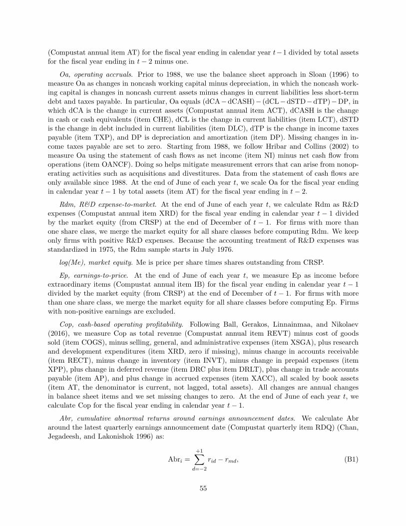
(Compustat annual item AT) for the fiscal year ending in calendar year t−1 divided by total assetsfor the fiscal year ending in t− 2 minus one.

Oa, operating accruals. Prior to 1988, we use the balance sheet approach in Sloan (1996) tomeasure Oa as changes in noncash working capital minus depreciation, in which the noncash work-ing capital is changes in noncash current assets minus changes in current liabilities less short-termdebt and taxes payable. In particular, Oa equals (dCA−dCASH)− (dCL−dSTD−dTP)−DP, inwhich dCA is the change in current assets (Compustat annual item ACT), dCASH is the changein cash or cash equivalents (item CHE), dCL is the change in current liabilities (item LCT), dSTDis the change in debt included in current liabilities (item DLC), dTP is the change in income taxespayable (item TXP), and DP is depreciation and amortization (item DP). Missing changes in in-come taxes payable are set to zero. Starting from 1988, we follow Hribar and Collins (2002) tomeasure Oa using the statement of cash flows as net income (item NI) minus net cash flow fromoperations (item OANCF). Doing so helps mitigate measurement errors that can arise from nonop-erating activities such as acquisitions and divestitures. Data from the statement of cash flows areonly available since 1988. At the end of June of each year t, we scale Oa for the fiscal year endingin calendar year t− 1 by total assets (item AT) for the fiscal year ending in t− 2.

Rdm, R&D expense-to-market. At the end of June of each year t, we calculate Rdm as R&Dexpenses (Compustat annual item XRD) for the fiscal year ending in calendar year t − 1 dividedby the market equity (from CRSP) at the end of December of t − 1. For firms with more thanone share class, we merge the market equity for all share classes before computing Rdm. We keeponly firms with positive R&D expenses. Because the accounting treatment of R&D expenses wasstandardized in 1975, the Rdm sample starts in July 1976.

log(Me), market equity. Me is price per share times shares outstanding from CRSP.

Ep, earnings-to-price. At the end of June of each year t, we measure Ep as income beforeextraordinary items (Compustat annual item IB) for the fiscal year ending in calendar year t − 1divided by the market equity (from CRSP) at the end of December of t− 1. For firms with morethan one share class, we merge the market equity for all share classes before computing Ep. Firmswith non-positive earnings are excluded.

Cop, cash-based operating profitability. Following Ball, Gerakos, Linnainmaa, and Nikolaev(2016), we measure Cop as total revenue (Compustat annual item REVT) minus cost of goodssold (item COGS), minus selling, general, and administrative expenses (item XSGA), plus researchand development expenditures (item XRD, zero if missing), minus change in accounts receivable(item RECT), minus change in inventory (item INVT), minus change in prepaid expenses (itemXPP), plus change in deferred revenue (item DRC plus item DRLT), plus change in trade accountspayable (item AP), and plus change in accrued expenses (item XACC), all scaled by book assets(item AT, the denominator is current, not lagged, total assets). All changes are annual changesin balance sheet items and we set missing changes to zero. At the end of June of each year t, wecalculate Cop for the fiscal year ending in calendar year t− 1.

Abr, cumulative abnormal returns around earnings announcement dates. We calculate Abraround the latest quarterly earnings announcement date (Compustat quarterly item RDQ) (Chan,Jegadeesh, and Lakonishok 1996) as:

Abri =+1∑

d=−2

rid − rmd, (B1)

55

in which rid is stock i’s return on day d (with the earnings announced on day 0) and rmd is themarket index return. We cumulate returns until one (trading) day after the announcement dateto account for the one-day-delayed reaction to earnings news. rmd is the value-weighted marketreturn for the Abr deciles with NYSE breakpoints and value-weighted returns.

For a firm to enter our sample at the beginning of month t, we require the end of the fiscal quarterthat corresponds to its most recent Abr to be within six months prior to month t. We do so to ex-clude stale information on earnings. To avoid potentially erroneous records, we also require the earn-ings announcement date to be after the corresponding fiscal quarter end. Because quarterly earningsannouncement dates are largely unavailable before 1972, the Abr sample starts in January 1972.

Ilr, industry lead-lag effect in prior returns. We start with the Fama-French (1997) 49-industryclassifications. Excluding financial firms from the sample leaves 45 industries. Following Hou(2007), at the beginning of each month t, we calculate Ilr as the month t− 1 value-weighted returnof the portfolio consisting of the 30% biggest (market equity) firms within a given industry.

Nop, net payout yield. Per Boudoukh, Michaely, Richardson, and Roberts (2007), total payoutsare dividends on common stock (Compustat annual item DVC) plus repurchases. Repurchases arethe total expenditure on the purchase of common and preferred stocks (item PRSTKC) plus anyreduction (negative change over the prior year) in the value of the net number of preferred stocksoutstanding (item PSTKRV). Net payouts equal total payouts minus equity issuances, which arethe sale of common and preferred stock (item SSTK) minus any increase (positive change over theprior year) in the value of the net number of preferred stocks outstanding (item PSTKRV). At theend of June of each year t, we measure Nop for the fiscal year ending in calendar year t− 1 dividedby the market equity (from CRSP) at the end of December of t − 1. For firms with more thanone share class, we merge the market equity for all share classes. Firms with zero net payouts areexcluded. Because the data on total expenditure and the sale of common and preferred stocks startin 1971, the Nop sample starts in July 1972.

Dac, discretionary accruals. We measure Dac using the modified Jones model from Dechow,Sloan, and Sweeney (1995):

Oai,tAi,t−1

= α11

Ai,t−1+ α2

dSALEi,t − dRECi,t

Ai,t−1+ α3

PPEi,t

Ai,t−1+ ei,t, (B2)

in which Oai,t is operating accruals for firm i, At−1 is total assets (Compustat annual item AT)at the end of year t− 1, dSALEi,t is the annual change in sales (item SALE) from year t− 1 to t,dRECi,t is the annual change in net receivables (item RECT) from year t − 1 to t, and PPEi,t isgross property, plant, and equipment (item PPEGT) at the end of year t. We estimate the cross-sectional regression (B2) for each two-digit SIC industry and year combination, formed separatelyfor NYSE/AMEX firms and for NASDAQ firms. We require at least six firms for each regression.The discretionary accrual for stock i is defined as the residual from the regression, ei,t. At the endof June of each year t, we calculate Dac for the fiscal year ending in calendar year t− 1.

Nsi, net stock issues. At the end of June of year t, we measure net stock issues, Nsi, as thenatural log of the ratio of the split-adjusted shares outstanding at the fiscal year ending in cal-endar year t − 1 to the split-adjusted shares outstanding at the fiscal year ending in t − 2. Thesplit-adjusted shares outstanding is shares outstanding (Compustat annual item CSHO) times theadjustment factor (item AJEX).

△I/Aqτ , τ = 1, 2, 3, 4, 8, 12, quarterly changes in investment-to-assets. For each month t, we

56

measure △I/Aqτ as the one-quarter asset growth for the τth quarter in the future and the one-

quarter asset growth for the latest fiscal quarter ending at least four months ago. Quarterly assetgrowth (investment-to-assets) quarterly total assets (Compustat quarterly item ATQ) divided byone-quarter-lagged total assets minus one.

C Estimating the Implied Cost of Capital

C.1 The Gebhardt, Lee, and Swaminathan (2001) Procedure

We measure current book equity, Bet, using the latest accounting data from the fiscal year end-ing between March of year t − 1 to February of t. This practice implies that for the IRR es-timates at the end of June in t, we impose at least a four-month lag to ensure that the ac-counting information is released to the public. The definition of book equity follows Davis,Fama, and French (2000). We apply clean surplus accounting to construct future book equityas Bet+τ = Bet+τ−1 + Bet+τ−1Et[Roet+τ ](1 − k), 1 ≤ τ ≤ 11, in which k is the dividend payoutratio in year t. Dividend payout ratio is dividends (Compustat annual item DVC) divided by earn-ings (item IB) for profitable firms, or dividends divided by 6% of total assets (item AT) for firmswith zero or negative earnings. We drop a firm if its book equity is zero or negative in any year.

We construct the expected Roe for the first three years ahead, using analyst earnings forecastsfrom the Institutional Brokers’ Estimated System (IBES) or forecasts from cross-sectional regres-sions. After year t + 3, we assume that the expected firm-level Roe mean-reverts linearly to thehistorical industry median Roe by year t+ 12, and becomes a perpetuity afterwards. We use theFama-French (1997) 48 industry classification. We use at least five and up to ten years of past Roedata from non-loss firms to compute the industry median Roe.

Following GLS (2001), we implement the GLS model on a per share basis with analysts’ earn-ings forecasts. Pt is the June-end share price from CRSP. Bet is book equity per share calculated asbook equity divided by the number of shares outstanding reported in June from IBES (unadjustedfile, item SHOUT). When IBES shares are not available, we use shares from CRSP (daily itemSHROUT) on the IBES pricing date (item PRDAYS) that corresponds to the IBES report.

At the end of June in each year t, we construct the expected ROE for year t + 1 to t + 3 asEt[Roet+τ ] = FEPSt+τ/Bet+τ−1, in which FEPSt+τ is the consensus mean forecast of earningsper share from IBES (unadjusted file, item MEANEST) for year t + τ (fiscal period indicator= τ) reported in June of t. We require the availability of earnings forecast for years t + 1 andt + 2. When the forecast for year t + 3 is not available, we use the long-term growth rate (itemLTG) to compute a three-year-ahead forecast: FEPSt+3 = FEPSt+2 × (1 + LTG). If the long-term growth rate is missing, we replace it with the growth rate implied by the first two forecasts:FEPSt+3 = FEPSt+2 × (FEPSt+2/FEPSt+1), when FEPSt+1 and FEPSt+2 are both positive.

As noted, we measure current book equity Bet based on the latest accounting data from thefiscal year ending between March of year t− 1 and February of t. However, firms with fiscal yearsending between March of t and May of t can announce their latest earnings before the IBES reportin June of t. In response to earnings announcement for the current fiscal year, the analyst forecastswould “roll forward” to the next year. As such, we also need to roll forward book equity by oneyear for these firms to match with the updated analyst forecasts. In particular, we roll forwardtheir book equity using clean surplus accounting as: Bet−1 + Yt−Dt, in which Bet−1 is the laggedbook equity (relative to the announced earnings), Yt is the earnings announced after February of tbut before the IBES report in June of t, and Dt is dividends.

57

In the first modified procedure, we follow Hou, van Dijk, and Zhang (2012) to estimate theIRRs at the firm level (not the per share basis), whenever regression-based earnings forecasts (notanalysts’ earnings forecasts) are used. We use pooled cross-sectional regressions to forecast futureearnings for up to three years ahead:

Yis+τ = a+ b1Ais + b2Dis + b3DDis + b4Yis + b5Y−is + b6ACis + ǫis+τ , (C1)

for 1 ≤ τ ≤ 3, in which Yis is earnings (Compustat annual item IB) of firm i for fiscal year s, Ais

is total assets (item AT), Dis is dividends (item DVC), and DDis is a dummy variable that equalsone for dividend payers, and zero otherwise. Y −

is is a dummy variable that equals one for negativeearnings, and zero otherwise, and ACis is operating accruals.

Prior to 1988, we use the balance-sheet approach of Sloan (1996) to measure operating accrualsas changes in noncash working capital minus depreciation, in which the noncash working capital ischanges in noncash current assets minus changes in current liabilities less short-term debt and taxespayable. In particular, AC = (△CA−△CASH)−(△CL−△STD−△TP )−DP , in which △CA isthe change in current assets (Compustat annual item ACT), △CASH is the change in cash or cashequivalents (item CHE), △CL is the change in current liabilities (item LCT), △STD is the changein debt included in current liabilities (item DLC, zero if missing), △TP is the change in incometaxes payable (item TXP, zero if missing), and DP is depreciation and amortization (item DP,zero if missing). Starting from 1988, we follow Hribar and Collins (2002) to measure AC using thestatement of cash flows as net income (item NI) minus net cash flow from operations (item OANCF).

In equation (C1), regressors with time subscript s are from the fiscal year ending between Marchof year s and February of s+ 1. Following Hou, van Dijk, and Zhang (2012), we winsorize all thelevel variables in equation (C1) at the 1st and 99th percentiles of their cross-sectional distributionseach year. In June of each year t, we estimate the regressions using the pooled panel data fromthe previous ten years. With a minimum four-month lag, the accounting data are from fiscal yearsending between March of t− 10 and February of t. Differing from the baseline GLS procedure, weforecast the expected earnings as the estimated regression coefficients times the latest values of the(unwinsorized) predictors from the fiscal year ending between March of t− 1 and February of t.

In the second modified procedure, we use annual cross-sectional regressions per Tang, Wu, andZhang (2014) to forecast the future ROE for up to three years, Roeis+τ ≡ Yis+τ/Beis+τ−1:

Roeis+τ = a+ b1 log

(

BeisPis

)

+ b2 log(Pis) + b3Y−is + b4Roeis + b5

Ais −Ais−1

Ais−1+ ǫis+τ , (C2)

for 1 ≤ τ ≤ 3, in which Roeis is return on equity of firm i for fiscal year s, Yis is earnings (Com-pustat annual item IB), Beis is the book equity, Pis is the market equity at the fiscal year endfrom Compustat or CRSP, Y −

is is a dummy variable that equals one for negative earnings and zerootherwise, and Ais is total assets (item AT). Regression variables with time subscript s are fromthe fiscal year ending between March of year s and February of s+ 1. Extremely small firms tendto have extreme regression variables which can affect the Roe regression estimates significantly. Toalleviate this problem, we exclude firm-years with total assets less than $5 million or book equityless than $2.5 million. Fama and French (2006, p. 496) require firms to have at least $25 milliontotal assets and $12.5 million book equity, but state that their results are robust to using the $5million total assets and $2.5 million book equity cutoff. We choose the less restrictive cutoff toenlarge the sample coverage. We also winsorize each variable (except for Y −

it ) at the 1st and 99thpercentiles of its cross-sectional distribution each year to further alleviate the impact of outliers.

58

In June of each year t, we run the regression (C2) using the previous ten years of data. Witha minimum four-month information lag, the accounting data are from fiscal years ending betweenMarch of t− 10 and February of t. Differing from the baseline GLS procedure, we directly forecastthe expected Roe, Et[Roet+τ ], as the average cross-sectional regression coefficients times the latestvalues of the predictors from fiscal years ending between March of t − 1 and February of t. Weimplement this modified GLS procedure at the firm level.

C.2 The Easton (2004) Procedure

Expected earnings are based on analyst forecasts from IBES or forecasts from regression models.Expected dividends are expected earnings times the current dividend payout ratio, which is com-puted as dividends (Compustat annual item DVC) divided by earnings (item IB) for profitable firms,or dividends divided by 6% of total assets (item AT) for firms with zero or negative earnings. Whenequation (15) has two positive roots (in very few cases), we use the average as the IRR estimate.

Following Easton (2004), we implement the model on the per share basis with analysts’ earningsforecasts. We measure Pt as the June-end share price from CRSP. At the end of June in year t, theexpected earnings per share for year t + τ is the consensus mean forecast from IBES (unadjustedfile, item MEANEST) for year t+ τ (fiscal period indicator = τ) reported in June of t.

Instead of analysts’ earnings forecasts, we also use pooled cross-sectional regressions in equation(C1) to forecast future earnings for up to two years ahead. In June of each year t, we estimate theregression using the pooled panel data from the previous ten years. With a four-month informationlag, the accounting data are from fiscal years ending between March of t − 10 and February of t.We construct the expected earnings as the estimated regression coefficients times the latest valuesof the (unwinsorized) predictors from the fiscal year ending between March of t− 1 and Februaryof t. We implement the modified procedure at the firm level.

Finally, we also use annual cross-sectional regressions in equation (C2) to forecast future ROEfor up to two years ahead. In June of each year t, we estimate the regression using the previousten years of data. With a four-month information lag, the accounting data are from fiscal yearsending between March of t − 10 and February of t. We forecast the expected Roe, Et[Roet+τ ],as the average regression coefficients times the latest values of the predictors from fiscal yearsending between March of t − 1 and February of t. Expected earnings are then constructed as:Et[Yt+τ ] = Et[Roet+τ ] × Bet+τ−1, in which Bet+τ−1 is the book equity in year t + τ − 1. Wemeasure current book equity Bet based on the latest accounting data from the fiscal year ending inMarch of t−1 to February of t, and impute future book equity by applying clean surplus accountingrecursively. We implement the modified procedure at the firm level.

C.3 The Claus and Thomas (2001) Procedure

We measure book equity, Bet, using the latest accounting data from the fiscal year ending betweenMarch of year t−1 and February of t. The definition of book equity follows Davis, Fama, and French(2000). We apply clean surplus accounting to construct future book equity as Bet+τ = Bet+τ−1 +Bet+τ−1Et[Roet+τ ](1 − k), 1 ≤ τ ≤ 4, in which k is the dividend payout ratio in year t. Dividendpayout ratio is dividends (Compustat annual item DVC) divided by earnings (item IB) for profitablefirms, or dividends divided by 6% of total assets (item AT) for firms with zero or negative earnings.We drop a firm if its book equity is zero or negative in any year. We construct the expected Roe,Et[Roet+τ ], for up to five years ahead, using analysts’ earnings forecasts from IBES or regression-based forecasts. Following CT (2001), we set g to the ten-year Treasury bond rate minus 3%.

59

Following CT (2001), we implement the CT model on the per share basis when using analysts’earnings forecasts. We measure Pt as the June-end share price from CRSP. Book equity pershare, Bt, is book equity divided by the number of shares outstanding reported in June from IBES(unadjusted file, item SHOUT). When IBES shares are not available, we use shares from CRSP(daily item SHROUT) on the IBES pricing date (item PRDAYS) that corresponds to the IBESreport. As noted, current book equity Bt is based on the latest accounting data from the fiscal yearending between March of t− 1 and February of t. However, firms with fiscal year ending in Marchof t to May of t can announce their latest earnings before the IBES report in June of t. To matchthe updated analyst forecasts, we roll forward their book equity using clean surplus accounting as:Bt−1+Yt−Dt, in which Bt−1 is the lagged book equity (relative to the announced earnings), Yt is theearnings announced after February of t but before the IBES report in June of t, and Dt is dividends.

At the end of June in each year t, we construct the expected Roe for year t + 1 to t + 5 asEt[Roet+τ ] = FEPSt+τ/Bet+τ−1, in which FEPSt+τ is the consensus mean forecast of earnings pershare from IBES (unadjusted file, item MEANEST) for year t + τ (fiscal period indicator = τ)reported in June of t. We require the availability of earnings forecast for years t + 1 and t + 2.When the forecast after year t+ 2 is not available, we use the long-term growth rate (item LTG)to construct it as FEPSt+τ = FEPSt+τ−1 × (1 + LTG). If the long-term growth rate is missing,we replace it with the growth rate implied by the forecasts for the previous two years: FEPSt+τ =FEPSt+τ−1 × (FEPSt+τ−1/FEPSt+τ−2), when FEPSt+τ−2 and FEPSt+τ−1 are both positive.

Instead of analysts’ earnings forecasts, we also use pooled cross-sectional regressions in equation(C1) to forecast future earnings for up to five years ahead. In June of each year t, we estimate theregression using the pooled panel data from the previous ten years. With a four-month informationlag, the accounting data are from fiscal years ending between March of t−10 and February of t. Weforecast the expected earnings as the estimated regression coefficients times the latest values of the(unwinsorized) predictors from the fiscal year ending between March of t−1 and February of t. Weimplement this modified CT procedure at the firm level. Finally, we also use annual cross-sectionalregressions in equation (C2) to forecast future Roe for up to five years ahead. In June of each yeart, we estimate the regression using the previous ten years of data. With a four-month informationlag, the accounting data are from fiscal years ending between March of t − 10 and February of t.We directly forecast the expected Roe, Et[Roet+τ ], as the average cross-sectional regression coeffi-cients times the latest values of the predictors from fiscal years ending between March of t− 1 andFebruary of t. We implement the modified CT procedure at the firm level.

C.4 The Ohlson and Juettner-Nauroth (2005) Procedure

Expected earnings are based on analyst forecasts from IBES or forecasts from regression models.Expected dividends are expected earnings times the current dividend payout ratio, which iscomputed as dividends (Compustat annual item DVC) divided by earnings (item IB) for profitablefirms, or dividends divided by 6% of total assets (item AT) for firms with zero or negative earnings.We follow Gode and Mohanram (2003) and use the average of forecasted near-term growth rateand five-year growth rate as an estimate of g. We require Et[Yt+2] and Et[Yt+4] to be positive sothat g is well defined. Following Gode and Mohanram (2003), we implement the OJ model on theper share basis with analysts’ earnings forecasts. We measure Pt as the June-end share price fromCRSP. At the end of June in year t, the expected earnings per share for year t+ τ is the consensusmean forecast from IBES (unadjusted file, item MEANEST) for year t+ τ (fiscal period indicator= τ) reported in June of t. We require the availability of earnings forecast for years t+1 and t+2.

60

When the forecast after year t+ 2 is not available, we use the long-term growth rate (item LTG)to construct it as: FEPSt+τ = FEPSt+τ−1 × (1 + LTG). If the long-term growth rate is missing,we replace it with the growth rate implied by the forecasts for the previous two years: FEPSt+τ =FEPSt+τ−1 × (FEPSt+τ−1/FEPSt+τ−2), when FEPSt+τ−2 and FEPSt+τ−1 are both positive.

Instead of analysts’ earnings forecasts, we also use pooled cross-sectional regressions in equation(C1) to forecast future earnings for up to five years ahead. In June of each year t, we estimate theregression using the pooled panel data from the previous ten years. With a four-month informationlag, the accounting data are from fiscal years ending between March of t − 10 and February of t.We construct the expected earnings as the estimated regression coefficients times the latest valuesof the (unwinsorized) predictors from the fiscal year ending between March of t− 1 and Februaryof t. We implement the modified OJ procedure at the firm level.

We also use annual cross-sectional regressions in equation (C2) to forecast future Roe for upto five years ahead. In June of each year t, we estimate the regression using the previous tenyears of data. With a four-month information lag, the accounting data are from fiscal years endingbetween March of t − 10 and February of t. We forecast the expected Roe, Et[Roet+τ ], as theaverage cross-sectional regression coefficients times the latest values of the predictors from fiscalyears ending between March of t − 1 and February of t. Expected earnings are then constructedas: Et[Yt+τ ] = Et[Roet+τ ] × Bet+τ−1, in which Bet+τ−1 is the book equity in year t + τ − 1. Wemeasure current book equity Bet based on the latest accounting data from the fiscal year ending inMarch of t−1 to February of t, and impute future book equity by applying clean surplus accountingrecursively. We implement the modified OJ procedure at the firm level.

61