Replicating Anomalies

Kewei Hou∗

The Ohio State University

and CAFR

Chen Xue†

University of Cincinnati

Lu Zhang‡

The Ohio State University

and NBER

June 2017 §

Abstract

The anomalies literature is infested with widespread p-hacking. We replicate thisliterature by compiling a large data library with 447 anomalies. With microcapsalleviated via NYSE breakpoints and value-weighted returns, 286 anomalies (64%)including 95 out of 102 liquidity variables (93%) are insignificant at the 5% level.Imposing the t-cutoff of three raises the number of insignificance to 380 (85%). Evenfor the 161 significant anomalies, their magnitudes are often much lower than originallyreported. Among the 161, the q-factor model leaves 115 alphas insignificant (150 witht < 3). In all, capital markets are more efficient than previously recognized.

∗Fisher College of Business, The Ohio State University, 820 Fisher Hall, 2100 Neil Avenue, Columbus OH 43210;and China Academy of Financial Research (CAFR). Tel: (614) 292-0552 and e-mail: hou.28@osu.edu.

†Lindner College of Business, University of Cincinnati, 405 Lindner Hall, Cincinnati, OH 45221. Tel: (513)556-7078 and e-mail: xuecx@ucmail.uc.edu.

‡Fisher College of Business, The Ohio State University, 760A Fisher Hall, 2100 Neil Avenue, Columbus OH 43210;and NBER. Tel: (614) 292-8644 and e-mail: zhanglu@fisher.osu.edu.

§We have benefited from helpful comments of Georgios Skoulakis (discussant), Rene Stulz, Stijn van Nieuwerburgh,Michael Weisbach, and other seminar participants at Cubist Systematic Strategies, Ohio State University, Universityof Cincinnati, and the 6th Symposium on Intelligent Investing at Western University. All remaining errors are our own.

1 Introduction

This paper conducts a gigantic replication of the bulk of the published anomalies literature in finance

and accounting by compiling a largest-to-date data library with 447 anomaly variables. The list

includes 57, 68, 38, 79, 103, and 102 variables from the momentum, value-versus-growth, investment,

profitability, intangibles, and trading frictions categories, respectively. We use a consistent set of

replication procedures throughout. To control for microcaps (stocks that are smaller than the 20th

percentile of market equity for New York Stock Exchange, or NYSE, stocks), we form testing deciles

with NYSE breakpoints and value-weighted returns. We treat an anomaly as a replication success

if the average return of its high-minus-low decile is significant at the 5% level (t ≥ 1.96).

Our results indicate widespread p-hacking in the anomalies literature. Out of 447 anomalies,

286 (64%) are insignificant at the 5% level. Imposing the cutoff t-value of three proposed by Harvey,

Liu, and Zhu (2016) raises the number of insignificant anomalies further to 380 (85%).

The biggest casualty is the liquidity literature. In the trading frictions category that contains

mostly liquidity variables, 95 out of 102 variables (93%) are insignificant. Prominent variables

that do not survive our replication include the Jegadeesh (1990) short-term reversal; the Datar-

Naik-Radcliffe (1998) share turnover; the Chordia-Subrahmanyam-Anshuman (2001) coefficient of

variation for dollar trading volume; the Amihud (2002) absolute return-to-volume; the Acharya-

Pedersen (2005) liquidity betas; the Ang-Hodrick-Xing-Zhang (2006) idiosyncratic volatility, total

volatility, and systematic volatility; the Liu (2006) number of zero daily trading volume; and the

Corwin-Schultz (2012) high-low bid-ask spread. Several recently proposed friction variables are also

insignificant, including the Bali-Cakici-Whitelaw (2011) maximum daily return; the Adrian-Etula-

Muir (2014) financial intermediary leverage beta; and the Kelly-Jiang (2014) tail risk.

The distress anomaly is virtually nonexistent in our replication. The Campbell-Hilscher-Szilagyi

(2008) failure probability, the O-score and Z-score studied in Dichev (1998), and the Avramov-

Chordia-Jostova-Philipov (2009) credit rating produce mostly insignificant average return spreads.

1

Other influential and widely cited variables that are insignificant in our replication include

the Bhandari (1988) debt-to-market; the Lakonishok-Shleifer-Vishny (1994) five-year sales growth;

several of the Abarbanell-Bushee (1998) fundamental signals; the Diether-Malloy-Scherbina (2002)

dispersion in analysts’ forecast; the Gompers-Ishii-Metrick (2003) corporate governance index;

the Francis-LaFond-Olsson-Schipper (2004) earnings attributes, including persistence, smoothness,

value relevance, and conservatism; the Francis et al. (2005) accruals quality; the Richardson-Sloan-

Soliman-Tuna (2005) total accruals; and the Fama-French (2015) operating profits-to-book equity.

Even for significant anomalies, their magnitudes are often much lower than originally re-

ported. Famous examples include the Jegadeesh-Titman (1993) price momentum; the Lakonishok-

Shleifer-Vishny (1994) cash flow-to-price; the Sloan (1996) operating accruals; the Chan-Jegadeesh-

Lakonishok (1996) earnings momentum formed on standardized unexpected earnings, abnormal

returns around earnings announcements, and revisions in analysts’ earnings forecasts; the Cohen-

Frazzini (2008) customer momentum; and the Cooper-Gulen-Schill (2008) asset growth.

Why does our replication differ so much from original studies? The key word is microcaps. Fama

and French (2008) show that microcaps represent only 3% of the total market capitalization of the

NYSE-Amex-NASDAQ universe, but account for 60% of the number of stocks. Microcaps not only

have the highest equal-weighted returns, but also the largest cross-sectional standard deviations

in returns and anomaly variables among microcaps, small stocks, and big stocks. Many studies

overweight microcaps with equal-weighted returns, and often together with NYSE-Amex-NASDAQ

breakpoints, in portfolio sorts. Hundreds of studies also use Fama-MacBeth (1973) cross-sectional

regressions of returns on anomaly variables, assigning even higher weights to microcaps than equal-

weights in sorts. The reason is that regressions impose a linear functional form, making them more

susceptible to outliers, which most likely are microcaps. Alas, due to high costs in trading these

stocks, anomalies in microcaps are more apparent than real. More important, with only 3% of the

total market equity, the economic importance of microcaps is small, if not trivial.

2

Our low replication rate of only 36% is not due to our extended sample relative to the original

studies. Repeating our replication in the original, shorter samples, we find that 293 (66%) anoma-

lies are insignificant at the 5% level, including 24, 44, 13, 38, 81, and 93 across the momentum,

value-versus-growth, investment, profitability, intangibles, and trading frictions categories, respec-

tively. Imposing the t-cutoff of three raises the number of insignificance further to 387 (86.6%). The

total number of insignificance at the 5% level, 293, is even higher than 286 in our extended sample.

We then use the q-factor model to explain the 161 significant anomalies. The q-factor model

explains the bulk of the anomalies, but still leaves 46 alphas significant (11 with t ≥ 3). Examples

include abnormal returns around earnings announcements, operating and discretionary accruals,

cash-based operating profits-to-assets, R&D-to-market, and the Heston-Sadka (2008) seasonality

anomalies. These anomalies tend to be relatively diffused, and do not comove strongly together.

Our contribution is to provide the largest-to-date replication in finance. Using a multiple testing

framework, Harvey, Liu, and Zhu (2016) cast doubt on the credibility of the anomalies literature,

and conclude that “most claimed research findings in financial economics are likely false (p. 5).”

Harvey et al. do not attempt to replicate the anomalies. In contrast, we replicate the bulk of the pub-

lished anomalies literature with a common set of procedures. We also present extensive evidence on

the relative successes and weaknesses of the q-factor model in explaining the significant anomalies.

The rest of the paper is organized as follows. Section 2 reviews the related literature on repli-

cation, and motivates our massive effort. Section 3 constructs the 447 anomalies, and details our

replication results. Section 4 uses the q-factor model to explain the significant anomalies. Finally,

Section 5 summarizes our results, and discusses their implications for future work.

2 Motivating Replication

Because replication is relatively new in finance, we briefly review the related literature.

3

2.1 Finance

Finance academics have long warned against data mining. Lo and MacKinlay (1990) argue that fu-

ture research is often motivated by the successes and failures of past investigations. As a result, few

empirical studies are free of data mining, which becomes more severe as the number of published

studies performed on a single data set increases. Fama (1998) shows that many anomalies tend to

weaken and even disappear when measured with value-weights. Conrad, Cooper, and Kaul (2003)

argue that data mining can account for up to one half of the in-sample relations between firm charac-

teristics and average returns in one-way sorts. Schwert (2003) shows that after anomalies are docu-

mented in the academic literature, the patterns often seem to disappear, reverse, or weaken. McLean

and Pontiff (2016) find that the average return spreads of 97 anomalies decline out of sample and

post publication, but the tests are based on NYSE-Amex-NASDAQ breakpoints and equal-weights.

As hundreds of anomalies have been documented in recent decades, the concern over data min-

ing has become especially acute. In a pioneering meta-study in finance, Harvey, Liu, and Zhu

(2016) present a new multiple testing framework to derive threshold statistical significant levels to

account for data mining in the anomalies literature. The threshold cutoff increases over time as

more anomalies have been data-mined. A newly discovered factor today should have a t-statistic

exceeding three. Reevaluating 296 significant anomalies in past published studies, Harvey et al.

report that 80–158 (27%–53%) are false discoveries, depending on the specific methods of adjusting

for multiple testing. The estimates are likely conservative because many factors have been tried by

empiricists, failed, and never been reported (and consequently unobservable).

Harvey, Liu, and Zhu (2016) suggest that two publication biases are likely responsible for the

high percentage of false discoveries. The first bias is that it is difficult to publish a negative result

in top academic journals. The second, more subtle bias is that it is difficult to publish replication

studies in finance and economics, while in many other scientific fields, replications routinely appear

in top journals. As a result, financial economists tend to focus on publishing new factors rather

4

than rigorously verifying the validity of published factors.

Harvey (2017) elaborates the complex agency problem behind the publication biases. Journal

editors compete for citation-based impact factors, and prefer to publish papers with the most signif-

icant results. In response to this incentive, authors often file away papers with results that are weak

or negative, instead of submitting them for publication. More disconcertingly, authors often engage

in p-hacking, i.e., selecting sample criteria and test procedures until insignificant results become

significant. The likely outcome is an embarrassingly large number of false positives that cannot

be replicated in the future. Harvey provides a Bayesian p-value as a remedy that incorporates the

economic plausibility of the testable hypothesis as part of statistical inference.

Yan and Zheng (2017) form about 18,000 fundamental signals, use bootstrapping to quantify

data mining, and find that top signals exhibit superior forecasting power of returns above and

beyond sampling variation. By permutating 240 accounting variables with 15 base variables and

five different ways of scaling, Yan and Zheng include both published variables and those that have

likely been tried but not reported. However, Yan and Zheng construct high-minus-low deciles with

NYSE-Amex-NASDAQ, as opposed to NYSE breakpoints, allowing microcaps to populate extreme

deciles. This practice exaggerates anomaly profits, especially in equal-weighted returns.

The anomalies literature is the scientific foundation for quantitative asset management (Ang

2014). Since the mid-1990s, factors-based exchange traded funds (ETFs) have experienced spec-

tacular growth. ETFGI, an independent research and consultancy firm, reports that total assets

under management of ETFs and other exchanged traded products (ETPs) reach over four trillion

dollars worldwide and over 1.5 trillion dollars in the U.S. as of May 2017. As factor investing be-

comes increasingly important, the financial press has rightfully called into question the reliability of

the underlying academic research. For example, a Bloomberg article by Coy (2017) writes: “Most

investors have a vague sense they’re being ripped off. Here’s how it happens.” “[R]esearchers have

more knobs to twist in search of a prized ‘anomaly’—a subtle pattern in the data that looks like

5

it could be a moneymaker. They can vary the period, the set of securities under consideration, or

even the statistical method. Negative findings go in a file drawer; positive ones get submitted to a

journal (tenure!) or made into an ETF whose performance we rely on for retirement.”

2.2 Economics

Finance is only the latest field that starts to take replication of published results seriously. In

economics, Leamer (1983) exposes the fragility of empirical results to small specification changes,

and proposes to “take the con out of econometrics” by reporting extensive sensitivity analysis to

show how key results vary with perturbations in regression specification and in functional form. In

an influential study, Dewald, Thursby, and Anderson (1986) attempt to replicate empirical results

published at Journal of Money, Credit, and Banking, and find that inadvertent errors are so com-

monplace that the original results often cannot be reproduced.1 McCullough and Vinod (2003)

report that nonlinear maximization routines from different software packages often produce very

different estimates, and many articles published at American Economic Review fail to test their

solutions across different software packages. Chang and Li (2015) report a success rate of less than

50% from replicating 67 published papers from 13 economics journals, and Camerer et al. (2016)

show a success rate of 61% from replicating 18 studies in experimental economics.

Collecting more than 50,000 tests published in American Economic Review, Journal of Political

Economy, and Quarterly Journal of Economics, Brodeur, Le, Sangnier, and Zylberberg (2016) doc-

ument a troubling two-humped pattern of test statistics. The pattern features a first hump with

high p-values, a sizeable under-representation of p-values just above 5%, and a second hump with

p-values slightly below 5%. The evidence indicates p-hacking that authors search for specifications

that deliver just-significant results and ignore those that give just-insignificant results to make their

work more publishable. The two-humped shape is less visible in articles with theoretical models,

1Dewald, Thursby, and Anderson (1986) write: “The replication of research is an essential component of scientificmethodology. Only through replication of the results of others can scientists unify the disparate findings of variousresearchers in a discipline into a defensible, consistent, coherent body of knowledge (p. 600).”

6

with randomized control trials, and with tenured or older authors.2

2.3 Meta-science

A highly influential article by Ioannidis (2005) develops a theoretical model to show that most (more

than 50%) research findings are false for most designs and for most fields. Results are more likely to

be false when the studies in a field use smaller samples, when the effect magnitudes are smaller, when

there exist many but fewer theoretically predicted relations, when researchers have more degrees of

freedom in designs, variable definitions, and analytical methods, when there exist greater financial

and other interest and bias, and when more independent teams are involved in a field.

We briefly review Ioannidis’s (2005) theoretical arguments in two simplest cases. Let PPVi be

field i’s positive predictive value, or the fraction that its published empirical relations are true.

Let Ri be the ratio of true relations to false relations tested in the field, meaning that the ex ante

probability of a relation being true is Ri/(1+Ri). Let 1−βi be the statistical power of the tests, and

α be the significance level. Ioannidis shows that the probability of a true finding in field i equals:

PPVi =(1− βi)Ri

(1− βi)Ri + α. (1)

In addition, in the presence of bias, ui, defined as the likelihood that an author reports a false

relation as true above and beyond sampling variation, the probability of a true finding becomes:

PPVi =(1− βi)Ri + uiβRi

(1− βi)Ri + α+ uiβRi + ui(1− α). (2)

For a numerical illustration, we set the significance level, α, to be 0.05 by convention. Ioannidis,

Stanley, and Doucouliagos (2015) report that the median statistical power is only 18% or less from

64,076 estimates in more than 6,700 empirical studies in economics. The bulk of the anomalies lit-

erature uses monthly returns from the Center for Research in Security Prices (CRSP) and account-

2Reviewing the replication literature in economics, Christensen and Miguel (2016) write: “[A]n overall increasein replication research will serve a critical role in establishing the credibility of empirical findings in economics, andin equilibrium, will create stronger incentives for scholars to generate more reliable results (p. 24).”

7

ing information from Compustat. The sample size is larger than most empirical economic studies.

However, our estimation target is the elusive expected stock return, and its common proxy as the

average realized return is notoriously noisy (Fama and French 1997, Elton 1999). To get the ball

rolling, we set the power to be 0.4, or βi = 0.6, which more than doubles Ioannidis et al.’s estimate.

We set Ri = 0.5, which implies that, a priori, the number of true relations is one half of the

number of false relations tested in the anomalies literature. This Ri value is likely optimistic. For

decades, the anomalies literature is largely statistical in nature. Fama and French (1992) reject

the classic Capital Asset Pricing Model (CAPM, Sharpe 1964, Lintner 1965). Despite its theoret-

ical elegance, the Breeden (1979) consumption CAPM performs even worse than the CAPM, and

is rarely used in the anomalies literature. The Merton (1973) intertemporal CAPM gives rise to

multifactor models, but is silent on the state variables that predict future movements in investment

opportunities. Finally, the Ross (1976) arbitrage pricing theory is also silent about the factors that

describe the cross section of average returns. In this theoretical vacuum, empiricists are free to

explore hundreds of accounting, price, volume, and other variables, often with little or no a priori

hypothesizing as for why a given anomaly variable should predict future returns.

For the bias parameter, ui, we experiment with three values, 0.25, 0.5, and 0.75. Our sense

is that ui must be high in the anomalies literature. First, publication biases are well documented

elsewhere in economics and social sciences (De Long and Lang 1992, Card and Krueger 1995, Franco,

Malhotra, and Simonovits 2014). Second, empiricists have many degrees of freedom in exploiting

ambiguities in sample criteria, variable definitions, and empirical specifications, which are all tools of

chasing statistical significance (Section 3.1.1). Third, more significant results make a bigger splash,

and are more likely to lead to publications, as well as promotion, tenure, and prestige in academia.

Fourth, with trillions of dollars invested in factors-based ETFs (and quantitative hedge funds)

worldwide, the financial interest is overwhelming. Finally, armies of academics and practitioners

engage in searching for significant anomalies, each eager to beat competitors in claiming the first in a

discovery. The anomalies literature is most likely one of the biggest areas in finance and accounting.

8

With these parameters, βi = 0.6, Ri = 0.5, and α = 0.05, equation (1) implies a positive predic-

tive value of 80%, without bias. However, more problematically, with the low, median, and high bias

parameter values of 0.25, 0.5, and 0.75, equation (2) implies positive predictive values of only 49%,

40%, and 36%, respectively. Most anomalies are false. As such, although perhaps surprising at first

glance, our evidence that only 36% of anomalies can be replicated accords well with the theoretical

arguments of Ioannidis (2005) and the multiple testing results of Harvey, Liu, and Zhu (2016).

More broadly, replication failures have been widely documented across scientific disciplines in the

past decade. Fanelli (2010) reports that “positive” results increase down the hierarchy of sciences,

with hard sciences such as space science and physics at the top and soft sciences such as psychology,

economics, and business at the bottom. In oncology, Prinz, Schlange, and Asadullah (2011) report

that scientists at Bayer fail to reproduce two thirds of 67 published studies. Begley and Ellis (2012)

report that scientists at Amgen attempt to replicate 53 landmark studies in cancer research, but

reproduce the original results in only six. Freedman, Cockburn, and Simcoe (2015) estimate the eco-

nomic costs of irreproducible preclinical studies amount to about 28 billion dollars in the U.S. alone.

In psychology, Open Science Collaboration (2015), which consists of about 270 researchers, con-

ducts replications of 100 studies published in top three academic journals, and reports a success rate

of only 36%. Baker (2016) reports that 80% of the respondents in a survey of 1,576 scientists con-

ducted by Nature believe that there exists a reproducibility crisis in the published scientific litera-

ture. The surveyed scientists cover diverse fields such as chemistry, biology, physics and engineering,

medicine, earth sciences, and others. More than 70% of researchers have tried and failed to repro-

duce another scientist’s experiments, and more than 50% have failed to reproduce their own exper-

iments. Selective reporting, pressure to publish, and poor use of statistics are three leading causes.

On replication, Ioannidis (2012) writes: “The ability to self-correct is considered a hallmark of

science. However, self-correction does not always happen to scientific evidence by default. The tra-

jectory of scientific credibility can fluctuate over time, both for defined scientific fields and for science

9

at-large. History suggests that major catastrophes in scientific credibility are unfortunately possible

and the argument that ‘it is obvious that progress is made’ is weak. Careful evaluation of the current

status of credibility of various scientific fields is important in order to understand any credibility

deficits and how one could obtain and establish more trustworthy results. Efficient and unbiased

replication mechanisms are essential for maintaining high levels of scientific credibility (p. 645).”

3 Replication

We report our replication results in this section. Table 1 shows the list of 447 anomalies, including

57, 68, 38, 79, 103, and 102 variables from the momentum, value-versus-growth, investment, prof-

itability, intangibles, and trading frictions categories, respectively.3 Appendix A details variable

definitions and portfolio construction. Monthly returns are from CRSP and accounting information

from the Compustat Annual and Quarterly Fundamental Files. The sample is from January 1967

to December 2014. Financial firms and firms with negative book equity are excluded.

Section 3.1 describes our replication procedures. Section 3.2 details the anomalies that cannot

be replicated. Section 3.3 shows that even for significant anomalies, their magnitudes are often

much lower than originally reported. Section 3.4 reports supplementary replication results.

3.1 A Common Set of Replicating Procedures

To test whether an anomaly variable can forecast returns reliably, we form testing deciles with

NYSE breakpoints and value-weighted returns. For annually sorted testing deciles, we split all

stocks at the end of June of each year t into deciles based on, for instance, book-to-market at the

fiscal year ending in calendar year t − 1, and calculate decile returns from July of year t to June

of t + 1. For monthly sorted portfolios involving latest earnings data, we use earnings data in

3Our data library with 447 anomalies is among the largest in the existing literature. Green, Hand, and Zhang(2013) reference 330 anomaly papers, but code up only 39 variables. Green, Hand, and Zhang (2016) and McLeanand Pontiff (2016) program about 100 anomaly variables. Harvey, Liu, and Zhu (2016) compile a list of 316 papers,but many variables are macroeconomic in nature, such as aggregate consumption growth. Also, Harvey et al. do notattempt replication. As noted, Yan and Zheng (2017) form about 18,000 fundamental signals, but these are frompermutating 240 accounting variables with 15 base variables and five different ways of scaling.

10

Compustat quarterly files in the months immediately after the quarterly earnings announcement

dates. For monthly sorted portfolios involving quarterly accounting data other than earnings, we

impose a four-month lag between the fiscal quarter end and subsequent returns. Unlike earnings,

other quarterly items are typically not available upon earnings announcement dates. Many firms

announce their earnings for a given quarter through a press release, and then file SEC reports

several weeks later. In particular, Easton and Zmijewski (1993) document a median reporting lag

of 46 days for NYSE/Amex firms and 52 days for NASDAQ firms. Chen, DeFond, and Park (2002)

also report that only 37% of quarterly earnings announcements include balance sheet information.

For monthly sorted anomalies, we include three different holding periods (1-, 6-, and 12-month).

Chan, Jegadeesh, and Lakonishok (1996), for example, emphasize the short-lived nature of momen-

tum, by examining how momentum profits vary with the holding horizon. As such, it is economically

interesting to study how monthly sorted anomalies vary across different holding periods.

Following Beaver, McNichols, and Price (2007), we adjust monthly stock returns for delisting

returns by compounding returns in the month before delisting with delisting returns from CRSP.

When a delisting return is missing, we replace it with the mean of available delisting returns of the

same delisting type and stock exchange in the prior 60 months. Appendix B details our delisting

adjustment procedure. Adjusting for delisting returns has little impact on our empirical results.

3.1.1 Why Portfolio Sorts with NYSE Breakpoints and Value-weighted Returns

Empiricists in the anomalies literature have much flexibility in test designs. Some studies exclude

stocks with prices per share lower than $1 or $5. We do not impose such a sample screen because

low price stocks have little impact on the results from our robust portfolio construction procedures.

Many studies also equal-weight portfolio returns. We instead use value-weights, for several rea-

sons. First, value-weights accurately reflect the wealth effect experienced by investors (Fama 1998).

Second, microcaps are influential in equal-weighted returns. Microcaps are on average only 3% of

the market value of the NYSE-Amex-NASDAQ universe, but account for about 60% of the total

11

number of stocks (Fama and French 2008). Due to high transaction costs, anomalies in microcaps

are difficult to exploit in practice. Also, with only 3% of the total market value, the economic sig-

nificance of microcaps is trivial. Finally, building on Blume and Stambaugh (1983), Asparouhova,

Bessembinder, and Kalcheva (2013) show that microstructure frictions, such as bid-ask spreads,

nonsynchronous trading, discrete prices, and order imbalances, can bias upward cross-sectional

monthly mean equal-weighted returns. In contrast, the bias in value-weighted returns is minimal.

When forming portfolios, many studies use NYSE-Amex-NASDAQ breakpoints, as opposed to

NYSE breakpoints. We use NYSE breakpoints because the cross-sectional dispersion of anomaly

variables is the largest among microcaps. Fama and French (2008) show that microcaps have the

highest cross-sectional standard deviations of returns and many anomaly variables among micro,

small, and big stocks. With NYSE-Amex-NASDAQ breakpoints, microcaps typically account for

more than 60% of the stocks in extreme deciles. These microcaps can greatly inflate the anomalies,

especially when combined with equal-weights. In contrast, using NYSE breakpoints assigns a fair

number of small and big stocks into extreme deciles, alleviating the impact of microcaps.

Hundreds of anomaly studies use Fama-MacBeth (1973) cross-sectional regressions of returns

on anomaly variables. We opt to use portfolio sorts, for several reasons. First, cross-sectional

regressions, most often performed with ordinary least squares, can be dominated by microcaps

because of their plentifulness. The slopes in these regressions are returns to zero-investment

portfolios (Fama 1976). In this sense, cross-sectional regressions are analogous to sorts with NYSE-

Amex-NASDAQ breakpoints and equal-weights. Second, cross-sectional regressions in effect assign

even more weights to microcaps than equal-weights. Because regressions impose a linear functional

form between average returns and anomaly variables, regressions are more susceptible to outliers,

volatile returns and values of anomaly variables, which most likely belong to microcaps. In contrast,

the largely nonparametric sorts do not impose such a linear functional form. Using weighted least

squares with the market equity as weights alleviates the concern on equal-weights, but not NYSE-

Amex-NASDAQ breakpoints or the linear functional form. Third, the zero-investment portfolios

12

constructed from cross-sectional regressions often involve high turnover and extreme leverage,

especially with many regressors, making the portfolios hard to interpret in economic terms.

Finally, most important, cross-sectional regressions with many anomaly variables provide an ex-

cess amount of flexibility. Leamer and Leonard (1983) show that inferences from slopes estimated in

linear regressions are very sensitive to the underlying specification.4 For example, two individually

insignificant variables that are highly correlated can appear significant when used together. Because

the set of regressors included in a regression specification is ambiguous, it is common and perhaps

even acceptable to explore various specifications, to search for, and then report a combination that

yields “statistical significance” (Simmons, Nelson, and Simonsohn 2011). The likelihood that at

least one specification out of many that can produce a false positive at the 5% level can be substan-

tially greater then 5%. Based on survey evidence, John, Loewenstein, and Prelec (2012) suggest

that such questionable research practices seem to be the prevailing norm in psychology. Bruns

and Ioannidis (2016) also emphasize that the choice of control variables can be a major source of

p-hacking in observational research.5 We avoid this trap altogether by using univariate sorts.

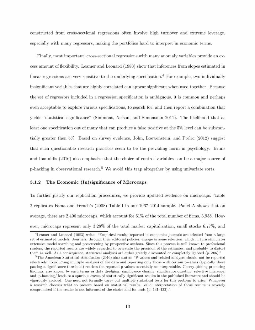
3.1.2 The Economic (In)significance of Microcaps

To further justify our replication procedures, we provide updated evidence on microcaps. Table

2 replicates Fama and French’s (2008) Table I in our 1967–2014 sample. Panel A shows that on

average, there are 2,406 microcaps, which account for 61% of the total number of firms, 3,938. How-

ever, microcaps represent only 3.28% of the total market capitalization, small stocks 6.77%, and

4Leamer and Leonard (1983) write: “Empirical results reported in economics journals are selected from a largeset of estimated models. Journals, through their editorial policies, engage in some selection, which in turn stimulatesextensive model searching and prescreening by prospective authors. Since this process is well known to professionalreaders, the reported results are widely regarded to overstate the precision of the estimates, and probably to distortthem as well. As a consequence, statistical analyses are either greatly discounted or completely ignored (p. 306).”

5The American Statistical Association (2016) also states: “P-values and related analyses should not be reportedselectively. Conducting multiple analyses of the data and reporting only those with certain p-values (typically thosepassing a significance threshold) renders the reported p-values essentially uninterpretable. Cherry-picking promisingfindings, also known by such terms as data dredging, significance chasing, significance questing, selective inference,and ‘p-hacking,’ leads to a spurious excess of statistically significant results in the published literature and should bevigorously avoided. One need not formally carry out multiple statistical tests for this problem to arise: Whenevera research chooses what to present based on statistical results, valid interpretation of those results is severelycompromised if the reader is not informed of the choice and its basis (p. 131–132).”

13

big stocks 90%. With equal-weights, microcaps earn on average 1.32% per month relative to 1.03%

for big stocks. In contrast, the value-weighted market return of 0.93% is close to 0.92% for big

stocks. More important, microcaps have the highest cross-sectional standard deviations of monthly

returns, 19.1%, followed by small stocks, 11.9%, and then by big stocks, 8.9%. Panel B shows

further that except for standardized unexpected earnings (Sue), the cross-sectional dispersions in

anomaly variables are the largest for microcaps, followed by small stocks, and then big stocks.

Figure 1 documents further that the economic significance of microcaps has declined in recent

decades. Panel A shows that microcaps account for 47.6% of firms at the beginning of the sample.

This fraction jumps to 66.6% in 1973 with the addition of NASDAQ, reaches to its maximum of

71.6% in 1987, and displays a downward trend afterward. At the end of 2014, microcaps account

for 46.8% of firms. In contrast, the numbers of small and big stocks show a upward trend since the

mid-1980s, and account for 26.1% and 27.1% of firms, respectively, at the end of our sample.

Panel B shows that microcaps represent 2.5% of the total market equity in 1967. This fraction

increases to 4.6% with the addition of NASDAQ, reaches its maximum of 6.2% in 1984, and shows

a downward trend afterward. At the end of 2014, microcaps represent only 1.4% of the total market

capitalization, in contrast to 5.6% for small stocks and 93% for big stocks. Panel C shows that

the breakpoints of microcaps and small stocks have increased over the years. At the end of 2014,

the 20th percentile of NYSE market equity is 595 million dollars, and the median is 2.7 billion

dollars. Finally, from 1973 to 2014, on average 77.5% of firms on NASDAQ are microcaps, which

represent 18.1% of the total NASDAQ market equity. At the end of 2014, 59.5% of NASDAQ firms

are microcaps, which represent only 2.9% of the total NASDAQ market equity (untabulated).

Our evidence that the economic weight of microcaps has declined in recent decades is consistent

with Kahle and Stulz (2017). Kahle and Stulz document that the percentage of small public firms

(defined as having market equity less than $100 million in 2015 dollars) has dropped dramatically,

from 61.5% in 1975 to 43.9% in 1995 and to 22.6% in 2015. The steady decrease in microcaps

14

accords well with both the low number of newly listed firms (Gao, Ritter, and Zhu 2013, Doidge,

Karolyi, and Stulz 2013) and the high number of delists (Doidge, Karolyi, and Stulz 2017).

3.1.3 What Is Replication?

Our replication procedures are consistent with the bulk of the replication literature in economics.

Building on Hunter (2001), Hamermesh (2007) defines three categories of replication. Pure replica-

tion is redoing a prior study in exactly the same way, statistical replication is the same statistical

model but different sample from the same underlying population, and scientific replication is differ-

ent sample, different population, and similar but not identical statistical model. Scientific replica-

tion “appears much more suited in type to our methods of research and, indeed, comprises most of

what economists view as replication (p. 716).” However, Clemens (2017) distinguishes replication

from robustness. Verification (replication) is defined as the same sample, population, and empirical

specification; reproduction (replication) as different sample from the same population but with the

same specification; reanalysis (robustness) as the same sample and population but different specifi-

cations; and extension (robustness) as different sample and population but the same specification.

We follow the bulk of the replication literature in economics in defining replication as “any

study whose primary purpose is to establish the correctness of a previous study” (see, for example,

The Replication Network, https://replicationnetwork.com).6 The articles on replication published

in the May 2017 issue of American Economic Review all adopt the same definition.7

6The Replication Network is endorsed by more than 370 economists worldwide as of May 2017.7In particular, Berry, Coffman, Hanley, Gihleb, and Wilson (2017) define a replication as “any project that

reports results that speak directly to the veracity of the original paper’s main hypothesis (p. 27).” Sukhtankar(2017) considers “all papers conforming to any of the Clemens (2017) classifications—including those he classifiesas robustness tests—as replications (p. 33).” Hamermesh (2017, p. 38) writes: “Applied microeconomics is not alaboratory science—at its best it consists of the generation of new ideas describing economic behavior, independentof time or space. The empirical validity of these ideas, after their relevance is first demonstrated for a particular timeand place, can only be usefully replicated at other times and places: If they are general descriptions of behavior,they should hold up beyond their original testing ground.” Finally, Duvendack, Palmer-Jones, and Reed (2017)operationalize replication as “any study whose main purpose is to determine the validity of one or more empiricalresults from a previously published study (p. 47).” Duvendack et al. further write: “By redoing the original dataanalysis, by adjusting model specifications, exploring the influence of unusual observations, using different estimationmethods, and alternative datasets, replication can identify spurious or fragile results (p. 46).”

15

3.2 Anomalies That Cannot be Replicated

We treat an anomaly as a replication failure if the average return of its high-minus-low decile is

insignificant at the 5% level (t < 1.96). This t-value cutoff is quite lenient from our perspective in

that we view a t-value no lower than 1.96 as a success. Despite our lax criterion, Table 3 reports

that 286 out of 447 anomaly variables (64%) earn insignificant average return spreads, including

20, 37, 11, 46, 77, and 95 anomalies from the momentum, value-versus-growth, investment, prof-

itability, intangibles, and trading frictions categories, respectively. Imposing the t-cutoff of three

increases the number of insignificance to 380 (85%), including 33, 61, 23, 66, 96, and 101 variables

across the six categories, respectively. In this subsection, we detail the insignificant anomalies, and

discuss possible procedural sources for their failed replications.

3.2.1 Momentum

Panel A of Table 3 reports 20 insignificant momentum anomalies. The high-minus-low Sue deciles

at the 6- and 12-month horizons earn on average 0.19% and 0.11% per month (t = 1.65 and 1.00),

respectively. These estimates are lower than those in Chan, Jegadeesh, and Lakonishok (1996),

who report 6- and 12-month buy-and-hold returns of 6.8% and 7.5%, respectively. The differences

likely arise because Chan et al. equal-weight the decile returns.

The high-minus-low revenue surprise (Rs) decile at the 6-month horizon earns an average return

of only 0.14% per month (t = 1.01). This estimate is lower than the average 6-month buy-and-

hold abnormal return of 4.42% for the high-minus-low quintile reported by Jegadeesh and Livnat

(2006), who use NYSE-Amex-NASDAQ breakpoints and equal-weighted returns. Also, Jegadeesh

and Livnat calculate abnormal returns against the size and book-to-market benchmark portfolios,

which are in turn value-weighted. The high-minus-low tax expense surprise (Tes) deciles at the

1-, 6-, and 12-month earn average returns of 0.26%, 0.28%, and 0.18% per month (t = 1.56, 1.9,

and 1.34), respectively. These estimates are lower than the average 3-month buy-and-hold return

of 3.9% reported by Thomas and Zhang (2011) based on NYSE-Amex-NASDAQ breakpoints and

16

equal-weighted returns. Also, the time lag between the fiscal quarter end and subsequent returns

is only three months, not four months in our construction.

The high-minus-low segment momentum (Sm) deciles at the 6- and 12-month earn only 0.09%

and 0.14% per month (t = 0.88 and 1.87), respectively. At the 1-month, Table 8 reports that the

average return is 0.59% (t = 2.57). The 0.59% estimate is lower than 0.95% reported in Cohen

and Lou (2012). Cohen and Lou use NYSE-Amex-NASDAQ breakpoints, and also impose a price

screen of $5 at portfolio formation. We use NYSE breakpoints with no price screen. We also show

that the average return is sensitive to the holding period.

Finally, the high-minus-low deciles formed on the industry lead-lag effect in earnings surprises

(Ile) at the 6- and 12-month earn on average 0.27% (t = 1.79) and 0.11% (t = 0.84), respectively.

In contrast, Hou (2007) shows stronger effects at shorter horizons using weekly cross-sectional re-

gressions. Table 4 shows that the high-minus-low Ile decile earns 0.62% (t = 3.7) at the 1-month,

and the industry lead-lag effect in prior returns (Ilr) is significant at all horizons.

3.2.2 Value-versus-growth

Panel B of Table 3 reports 37 insignificant value-versus-growth anomalies. Debt-to-market equity

(Dm) is insignificant in both annual sorts and monthly sorts at all horizons. The average returns

of the high-minus-low deciles vary from 0.27% to 0.32% per month, with t-values from 1.17 to 1.59.

The estimates contrast with Bhandari’s (1988) results from cross-sectional regressions. Dividend

yield (Dp) and payout yield (Op) are also insignificant in both annual sorts and all monthly sorts.

This evidence contrasts with Litzenberger and Ramaswamy’s (1979) results on Dp from cross-

sectional regressions, as well as Boudoukh, Michaely, Richardson, and Roberts’s (2007) results on

Op based on NYSE breakpoints but equal-weighted returns.

The high-minus-low five-year sales growth (Sr) decile earns an average return of only −0.2%

per month (t = −1.08), which is much lower in magnitude than −7.3% per annum in Lakonishok,

Shleifer, and Vishny (1994) based on NYSE-Amex breakpoints and equal-weighted returns (without

17

NASDAQ stocks). Net debt-to-price (Ndp) is insignificant in both annual sorts and monthly sorts at

all horizons, with average return spreads ranging from 0.17% to 0.31% per month, and t-values from

0.71 to 1.62. The average returns are lower than 8.7% per annum in Penman, Richardson, and Tuna

(2007) based on NYSE-Amex-NASDAQ breakpoints and equal-weighted size-adjusted returns.

3.2.3 Investment

Panel C of Table 3 reports 11 insignificant investment anomalies. The high-minus-low decile on

the Richardson-Sloan-Soliman-Tuna (2005) total accruals (Ta) earns an average return of −0.23%

(t = −1.63). In contrast, Richardson et al.’s Table 8 reports a negative slope of Ta more than six

standard errors from zero in cross-sectional regressions of returns. Their Table 10 also shows an

average (size-adjusted) return of −13.3% per annum (t = −10.25) for the high-minus-low decile

based on NYSE-Amex-NASDAQ breakpoints and equal-weights. The high-minus-low deciles on

net external finance (Nxf) and net equity finance (Nef) earn on average −0.27% and −0.17% per

month (t = −1.44 and −0.86), respectively. These estimates are lower in magnitude than −15.5%

(t = −5.7) and −11.2% (t = −3.82) per annum reported by Bradshaw, Richardson, and Sloan

(2006) based on NYSE-Amex-NASDAQ breakpoints and equal-weighted size-adjusted returns.

3.2.4 Profitability

Panel D of Table 3 reports 46 insignificant anomalies in the profitability category. The return on

equity (Roe) is significant mostly within short horizons. At the 6-month, the high-minus-low decile

earns on average 0.42% (t = 1.95), and at the 12-month, 0.24% (t = 1.19). At the 1-month, the

average return spread is 0.69% (t = 3.07) (Table 4). The evidence is largely consistent with Fama

and French (2006), who use annual sorts, and Hou, Xue, and Zhang (2015), who use monthly sorts.

Many different measures of profitability have recently been proposed to predict returns, but not

all are effective. The high-minus-low gross profits-to-lagged assets (Gla) decile earns an average

return of only 0.16% per month (t = 1.04). This average return is lower than that of 0.38% (t = 2.62)

for the high-minus-low gross profits-to-assets (Gpa) decile (Table 4). The difference between Gla

18

and Gpa is that Gla scales gross profits with one-period-lagged assets, but Gpa scales with current

assets. Because both profits and assets are measured at the end of a period in Compustat, profits

should be scaled by lagged assets, which in turn produce current profits. In contrast, the current

assets at the end of a period are accumulated through investment over the current period, and start

to generate profits only in future periods. Most important, because Gpa equals Gla divided by asset

growth (current assets-to-lagged assets), the Gpa effect is confounded with the investment effect.

Purging the investment effect yields an economically small and statistically insignificant Gla effect.

Perhaps surprisingly, operating profits-to-book equity (Ope), which is the sorting variable under-

lying the Fama-French (2015) robust-minus-weak (RMW) profitability factor, is also insignificant.

The high-minus-low Ope decile earns an average return of only 0.25% per month (t = 1.2). Ope

scales operating profits with the current book equity. Scaling with the one-period-lagged book

equity as in operating profits-to-lagged book equity (Ole) reduces the average return spread further

to 0.07% (t = 0.37). Ball, Gerakos, Linnainmaa, and Nikolaev (2015) add research and develop-

ment expenses to operating profits, show that the high-minus-low operating profits-to-assets (Opa)

decile earns on average 0.29% (t = 1.95). We replicate their result with an average return of

0.37% (t = 1.87). However, scaling their operating profits with the lagged assets as in operating

profits-to-lagged assets (Ola) reduces the average return to 0.2% (t = 1.07).

A bigger surprise is that the distress anomaly is virtually nonexistent in our replication. In an-

nual sorts, the high-minus-low failure probability (Fp) decile earns an average return of −0.38% per

month (t = −1.28) from July 1976 to December 2014. This estimate is much lower in magnitude

than −9.66% per annum reported by Campbell, Hilscher, and Szilagyi (2008) in the 1981–2003

sample. We replicate their estimate in their sample period with an average return of −0.82% per

month (t = −2.1). However, prior to their sample, the average return is strongly positive, 0.69%

from July 1976 to December 1980 (0.09% from 2003 onward). In monthly sorts, the average returns

are −0.48% and −0.36% at the 1- and 12-month, respectively, but both are within 1.5 standard

errors from zero. At the 6-month, the average return is −0.63% (t = −2.03) (Table 4). Finally,

19

while Campbell et al. use NYSE-Amex-NASDAQ breakpoints, we use NYSE breakpoints.

Several alternative measures of financial distress, including Altman’s (1968) Z-score (Z),

Ohlson’s (1980) O-score (O), and credit rating (Cr), show even weaker forecasting power than

failure probability. None of the high-minus-low deciles show any significant average returns in

either annual sorts or monthly sorts at any horizon. In particular, the average returns of the high-

minus-low O deciles range from −0.06% (t = −0.3) to −0.36% per month (t = −1.57), and those

of the high-minus-low Z deciles from 0.01% (t = 0.06) to −0.09% (t = −0.46). These estimates

contrast with those in Dichev (1998), who reports an average return of −1.17% (t = −3.36) for the

highest-10%-minus-lowest-70% O portfolio based on NYSE-Amex-NASDAQ breakpoints and equal-

weighted returns, as well as a significantly positive slope for Z-score in cross-sectional regressions.

Finally, the high-minus-low credit rating (Cr) deciles all earn average returns that are close

to zero at the 1-, 6-, and 12-month horizons. These estimates contrast with Avramov, Chordia,

Jostova, and Philipov (2009), who report a high-minus-low average return of −1.09% per month

(t = −2.61) based on NYSE-Amex-NASDAQ breakpoints and equal-weighted returns. Besides the

procedural difference, another difference is that Avramov et al. use credit ratings data from Ratings

Xpress, to which we do not have access because it has been discontinued on WRDS.

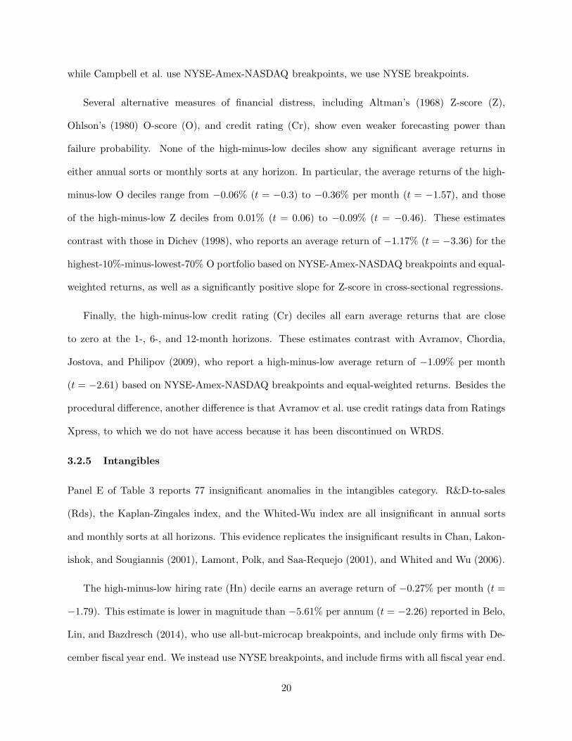
3.2.5 Intangibles

Panel E of Table 3 reports 77 insignificant anomalies in the intangibles category. R&D-to-sales

(Rds), the Kaplan-Zingales index, and the Whited-Wu index are all insignificant in annual sorts

and monthly sorts at all horizons. This evidence replicates the insignificant results in Chan, Lakon-

ishok, and Sougiannis (2001), Lamont, Polk, and Saa-Requejo (2001), and Whited and Wu (2006).

The high-minus-low hiring rate (Hn) decile earns an average return of −0.27% per month (t =

−1.79). This estimate is lower in magnitude than −5.61% per annum (t = −2.26) reported in Belo,

Lin, and Bazdresch (2014), who use all-but-microcap breakpoints, and include only firms with De-

cember fiscal year end. We instead use NYSE breakpoints, and include firms with all fiscal year end.

20

The average returns of the high-minus-low deciles on percentage change in sales minus that

in inventory (dSi), percentage change in sales minus that in accounts receivable (dSa), percentage

change in gross margin minus that in sales (dGs), percentage change in sales minus that in SG&A

(dSs), and labor force efficiency (Lfe) are all small and insignificant, ranging from 0.04% to 0.2%

per month, with t-values from 0.24 to 1.59. For comparison, Abarbanell and Bushee (1998) report

insignificant results for dSa, dGs, and Lfe, but significant results for dSi and dSs based on cross-

sectional regressions of size-adjusted buy-and-hold returns of up to 12 months. However, while

Abarbanell and Bushee report insignificant results for effective tax rate (Etr), its average return

spread is 0.25% (t = 2.35) in our replication (Table 4).

The high-minus-low corporate governance (Gind) decile earns a tiny average return of 0.02%

per month (t = 0.06) in our sample from September 1990 to December 2006 (the last available

date). In contrast, Gompers, Ishii, and Metrick (2003) report a significant high-minus-low Gind

decile alpha of −0.71% (t = −2.73) in the Carhart (1997) four-factor model in their sample from

September 1990 to December 1999. We come close to replicate their result, with a Carhart alpha

of −0.59% (t = −1.88) and an average return of −0.73% (t = −2.04) in their sample period. How-

ever, outside their sample from January 2000 to December 2006, the high-minus-low Gind decile

earns a positive average return of 1.01% (t = 2.09), and its Carhart alpha is insignificant, 0.2%

(t = 0.56). Our evidence is consistent with Core, Guay, and Rusticus (2006), who document that

the high-minus-low Gind return exhibits a reversal from 2000 to 2003.

The high-minus-low accruals quality (Acq) decile earns a tiny average return of −0.07% per

month (t = −0.36) in annual sorts, and the average returns from monthly sorts are quantitatively

close. The average returns of the high-minus-low deciles formed on earnings persistence (Eper),

earnings smoothness (Esm), value relevance of earnings (Evr), and earnings conservatism (Ecs)

are all small and insignificant, ranging from −0.06% to 0.18%, with t-values from −0.45 to 1.32.

These results contrast with Francis, LaFond, Olsson, and Schipper (2004, 2005), who report that

these earnings attributes have significant relations with the cost of equity. Francis et al. base their

21

inferences on ex ante accounting-based measures of cost of capital, not average realized returns.

Although Francis et al. construct factors based on the earnings attributes, their average returns

are not reported. Our evidence accords with Core, Guay, and Verdi (2008), who also report that

the accruals quality is not priced in asset pricing tests. We emphasize, however, that the two other

attributes in Francis et al., earnings predictability (Eprd) and earnings timeliness (Etl), do produce

significant average return spreads, −0.49% (t = −2.75) and 0.36% (t = 2.85), respectively (Table 4).

The high-minus-low deciles formed on dispersion of analysts’ earnings forecasts (Dis) earn

−0.24%,−0.22%, and −0.13% per month at the 1-, 6-, and 12-month, all of which are within

one standard error from zero. The evidence contrasts with Diether, Malloy, and Scherbina (2002),

who report an average return of −0.79% (t = −2.88) for the low-minus-high Dis quintile at the

1-month based on NYSE-Amex-NASDAQ breakpoints and equal-weighted returns. Diether et al.

also exclude stocks with prices per share lower than $5. We do not impose such a price screen.

3.2.6 Trading Frictions

The biggest casualty of our replication is the trading frictions (liquidity) category, with 95 out of

102 variables (93%) insignificant. Panel F of Table 3 shows that 15 out of 16 volatility measures

earn insignificant average returns for their high-minus-low deciles. In particular, the high-minus-low

deciles on idiosyncratic volatility calculated from the Fama-French (1993) three-factor model (Ivff)

earn on average −0.51%, −0.33%, and −0.18% per month (t = −1.62,−1.11, and −0.62) at the 1-,

6-, and 12-month, respectively. The high-minus-low deciles on total volatility (Tv) earn on average

−0.4%,−0.25%, and −0.2% (t = −1.16,−0.77, and −0.62) at the three horizons, respectively. The

systematic volatility risk (Sv) is insignificant at the 6- and 12-month (Table 3), but significant at

the 1-month with an average return of −0.53% (t = −2.47) (Table 4).

Our estimates are lower than −1.06%, −0.97%, and −1.04% per month (t = −3.1,−2.86 and

−3.9) for the high-minus-low Ivff, Tv, and Sv quintiles, respectively, all at the 1-month, reported

in Ang, Hodrick, Xing, and Zhang (2006) based on NYSE-Amex-NASDAQ breakpoints and value-

22

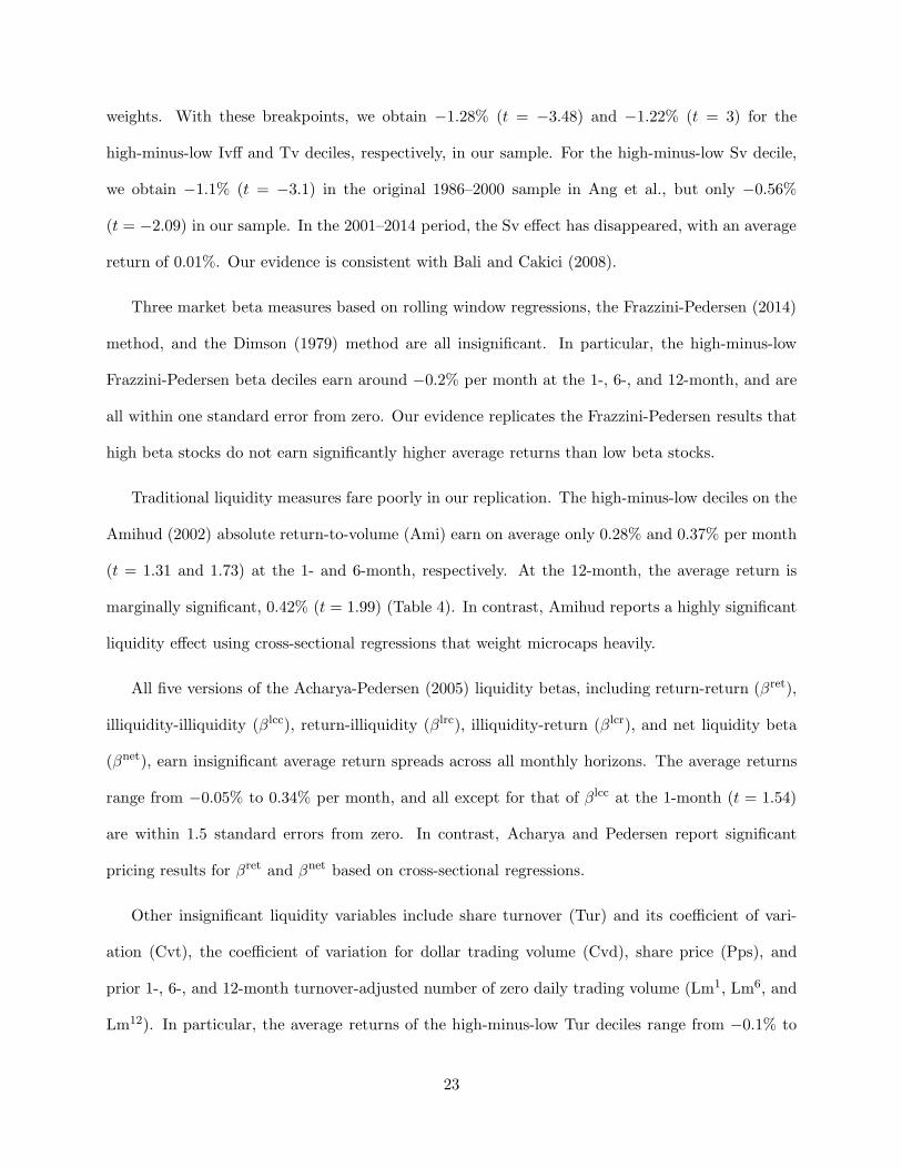
weights. With these breakpoints, we obtain −1.28% (t = −3.48) and −1.22% (t = 3) for the

high-minus-low Ivff and Tv deciles, respectively, in our sample. For the high-minus-low Sv decile,

we obtain −1.1% (t = −3.1) in the original 1986–2000 sample in Ang et al., but only −0.56%

(t = −2.09) in our sample. In the 2001–2014 period, the Sv effect has disappeared, with an average

return of 0.01%. Our evidence is consistent with Bali and Cakici (2008).

Three market beta measures based on rolling window regressions, the Frazzini-Pedersen (2014)

method, and the Dimson (1979) method are all insignificant. In particular, the high-minus-low

Frazzini-Pedersen beta deciles earn around −0.2% per month at the 1-, 6-, and 12-month, and are

all within one standard error from zero. Our evidence replicates the Frazzini-Pedersen results that

high beta stocks do not earn significantly higher average returns than low beta stocks.

Traditional liquidity measures fare poorly in our replication. The high-minus-low deciles on the

Amihud (2002) absolute return-to-volume (Ami) earn on average only 0.28% and 0.37% per month

(t = 1.31 and 1.73) at the 1- and 6-month, respectively. At the 12-month, the average return is

marginally significant, 0.42% (t = 1.99) (Table 4). In contrast, Amihud reports a highly significant

liquidity effect using cross-sectional regressions that weight microcaps heavily.

All five versions of the Acharya-Pedersen (2005) liquidity betas, including return-return (βret),

illiquidity-illiquidity (βlcc), return-illiquidity (βlrc), illiquidity-return (βlcr), and net liquidity beta

(βnet), earn insignificant average return spreads across all monthly horizons. The average returns

range from −0.05% to 0.34% per month, and all except for that of βlcc at the 1-month (t = 1.54)

are within 1.5 standard errors from zero. In contrast, Acharya and Pedersen report significant

pricing results for βret and βnet based on cross-sectional regressions.

Other insignificant liquidity variables include share turnover (Tur) and its coefficient of vari-

ation (Cvt), the coefficient of variation for dollar trading volume (Cvd), share price (Pps), and

prior 1-, 6-, and 12-month turnover-adjusted number of zero daily trading volume (Lm1, Lm6, and

Lm12). In particular, the average returns of the high-minus-low Tur deciles range from −0.1% to

23

−0.15% per month, all of which are within 0.6 standard errors from zero. In contrast, Datar, Naik,

and Radcliffe (1998) report highly significant pricing results for Tur in cross-sectional regressions

with only NYSE stocks. The average returns of the high-minus-low Cvd deciles vary from 0.1% to

0.18%, all of which are within 1.3 standard errors from zero. This evidence contrasts with Chor-

dia, Subrahmanyam, and Anshuman (2001), who report highly significant results for Cvd with

cross-sectional regressions with NYSE and Amex stocks. Finally, none of the three Lm measures

interacted with three holding periods (nine measures in total) produce any significance. The high-

minus-low average returns range from −0.07% to 0.38%, with t-values from −0.33 to 1.82. In

contrast, Liu (2006) reports significant average return spreads for eight out of the nine measures

using NYSE breakpoints but equal-weighted returns (without NASDAQ stocks).

The high-minus-low short-term reversal (Srev) decile earns on average only −0.26% per month

(t = −1.31). This estimate is much lower in magnitude than −1.99% (t = −12.55) reported in

Jegadeesh (1990) based on NYSE-Amex-NASDAQ breakpoints and equal-weighted returns. The

high-minus-low high-low bid-ask spread (Shl) deciles earn on average −0.16%,−0.16%, and −0.12%

at the 1-, 6-, and 12-month, which are all within 0.6 standard errors from zero. In contrast, Corwin

and Schultz (2012) report highly significant abnormal returns (three-factor alphas) of more than

1% by weighting decile returns based on prior-month returns, with weights closer to equal- than

value-weights. Also, Corwin and Schultz use only NYSE and Amex stocks with a price screen of $5.

Several recently proposed friction variables are also insignificant. The high-minus-low tail risk

(Tail) deciles earn on average 0.11%, 0.15%, and 0.19% per month (t = 0.57, 0.79, and 1.13) at the

1-, 6-, and 12-month, respectively. These estimates are lower than 0.36% (t = 2) at the 1-month

and 0.35% (t = 2.15) at the 12-month reported by Kelly and Jiang (2014) based on NYSE-Amex-

NASDAQ breakpoints. The high-minus-low deciles on maximum daily return (Mdr) earn on average

−0.34%,−0.17%, and −0.07% (t = −1.14,−0.62, and −0.24) across the three horizons, respectively.

These estimates are much lower in magnitude than −1.03% (t = −2.83) at the 1-month reported

in Bali, Cakici, and Whitelaw (2011) based on NYSE-Amex-NASDAQ breakpoints. In particular,

24

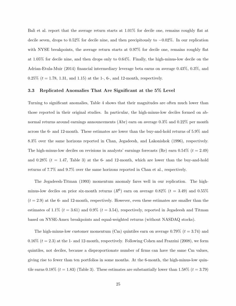
Bali et al. report that the average return starts at 1.01% for decile one, remains roughly flat at

decile seven, drops to 0.52% for decile nine, and then precipitously to −0.02%. In our replication

with NYSE breakpoints, the average return starts at 0.97% for decile one, remains roughly flat

at 1.05% for decile nine, and then drops only to 0.64%. Finally, the high-minus-low decile on the

Adrian-Etula-Muir (2014) financial intermediary leverage beta earns on average 0.43%, 0.3%, and

0.25% (t = 1.78, 1.31, and 1.15) at the 1-, 6-, and 12-month, respectively.

3.3 Replicated Anomalies That Are Significant at the 5% Level

Turning to significant anomalies, Table 4 shows that their magnitudes are often much lower than

those reported in their original studies. In particular, the high-minus-low deciles formed on ab-

normal returns around earnings announcements (Abr) earn on average 0.3% and 0.22% per month

across the 6- and 12-month. These estimates are lower than the buy-and-hold returns of 5.9% and

8.3% over the same horizons reported in Chan, Jegadeesh, and Lakonishok (1996), respectively.

The high-minus-low deciles on revisions in analysts’ earnings forecasts (Re) earn 0.54% (t = 2.49)

and 0.28% (t = 1.47, Table 3) at the 6- and 12-month, which are lower than the buy-and-hold

returns of 7.7% and 9.7% over the same horizons reported in Chan et al., respectively.

The Jegadeesh-Titman (1993) momentum anomaly fares well in our replication. The high-

minus-low deciles on prior six-month returns (R6) earn on average 0.82% (t = 3.49) and 0.55%

(t = 2.9) at the 6- and 12-month, respectively. However, even these estimates are smaller than the

estimates of 1.1% (t = 3.61) and 0.9% (t = 3.54), respectively, reported in Jegadeesh and Titman

based on NYSE-Amex breakpoints and equal-weighted returns (without NASDAQ stocks).

The high-minus-low customer momentum (Cm) quintiles earn on average 0.79% (t = 3.74) and

0.16% (t = 2.3) at the 1- and 12-month, respectively. Following Cohen and Frazzini (2008), we form

quintiles, not deciles, because a disproportionate number of firms can have the same Cm values,

giving rise to fewer than ten portfolios in some months. At the 6-month, the high-minus-low quin-

tile earns 0.18% (t = 1.83) (Table 3). These estimates are substantially lower than 1.58% (t = 3.79)

25

reported in Cohen and Frazzini (2008) based on NYSE-Amex-NASDAQ breakpoints as well as a

$5 price screen, albeit with value-weighted returns.

The high-minus-low cash flow-to-price (Cp) decile earns on average 0.49% per month (t = 2.47).

This average return is much lower than 9.9% per annum reported in Lakonishok, Shleifer, and

Vishny (1994) based on NYSE-Amex breakpoints and equal-weighted returns (without NASDAQ

stocks). Also, sorting on operating cash flow-to-price (Ocp) yields an average return spread of 0.77%

(t = 3.5), which is much lower than 14.9% per annum (t = 2.65) reported in Desai, Rajgopal, and

Venkatachalam (2004) based on NYSE-Amex-NASDAQ breakpoints and equal-weighted returns.

The high-minus-low asset growth (investment-to-assets, I/A) decile earns on average −0.46% per

month (t = −2.92). This average return is much lower in magnitude than −1.05% (t = −5.04) with

value-weighted returns and −1.73% (t = −8.45) with equal-weighted returns reported by Cooper,

Gulen, and Schill (2008), who use NYSE-Amex-NASDAQ breakpoints. Finally, the high-minus-low

operating accruals (Oa) decile earns only −0.27% (t = −2.13). This average return is much smaller

in magnitude than −10.4% per annum (t = −4.71) reported by Sloan (1996). Sloan uses NYSE-

Amex breakpoints (without NASDAQ stocks), equal-weighted returns, and size-adjusted abnormal

returns, in which the size-decile benchmark uses value-weighted returns.

3.4 Additional Results on Replication

In this subsection, we furnish supplementary results on replication, including average return spreads

in the original samples (Section 3.4.1), average return spreads with NYSE-Amex-NASDAQ break-

points and equal-weights (Section 3.4.2), and investment capacity of microcaps (Section 3.4.3).

3.4.1 Average Return Spreads in the Original Samples

We interpret the evidence in Table 3 that only 36% of anomalies can be replicated as indicative of

p-hacking, mainly by overweighting microcaps. An alternative interpretation is that the insignifi-

cant anomalies exist in the original samples examined in original studies, but have since attenuated,

26

perhaps due to time-varying expected returns and mispricing arbitrage. While we cannot rule it

out entirely, Table 5 based on the original samples casts doubt on this alternative interpretation.

The empirical design of Table 5 is identical to that of Tables 3 and 4, except that we stop the sam-

ple of a given anomaly at the sample end of its original study. If the start of the sample in the original

study is later than January 1967, we begin our sample at the same date. Otherwise, we start at Jan-

uary 1967, which is the earliest date in our sample, to be consistent with our later tests (Section 4).

Table 5 shows that out of 447 anomalies, 293 (66%) are insignificant at the 5% level, including

24, 44, 13, 38, 81, and 93 across the momentum, value-versus-growth, investment, profitability,

intangibles, and trading frictions categories, respectively. The evidence is largely similar to Table

3. The total number of insignificance, 293, is even higher than 286 in the full sample. Imposing

the t-cutoff of three raises the number of insignificance to 387 (86.6%), including 35, 64, 25, 66, 97,

and 100 across the six categories, respectively. Across the 154 significant anomalies at the 5% level

in the original samples, the average absolute return spread is 0.65% per month, and the average

absolute t-value is 2.89. For comparison, across the 161 significant anomalies in the full sample,

the average absolute return spread is 0.51%, and the average absolute t-value is 2.93.

Sampling variation plays a limited role. Once we extend the original samples to the full sample,

30 anomalies change from being significant to insignificant, but 37 anomalies from insignificant to

significant. Among the former group that loses significance in the full sample, the average return

spreads of five-year sales growth (Sr), O-score (O), F-score (F), and short-term reversal (Srev) are

−0.45%, −0.6%, 0.65%, and −0.65% per month (t = −1.99,−2.06, 2.19, and −2.4), respectively, in

their original samples. However, sample variation also helps 37 different anomalies gain significance

in the full sample. For example, the average return spreads of Sue at 1-month, revisions in ana-

lysts’ forecasts (Re) at 6-month, sales-to-price (Sp), analysts-based intrinsic value-to-market (Vfp),

percent operating accruals (Poa), R&D-to-market (Rdm), and total skewness (Ts) at 1-month are

all insignificant in the original samples, but become significant in the full sample.

27

3.4.2 Average Return Spreads with NYSE-Amex-NASDAQ Breakpoints and Equal-

weighted Returns

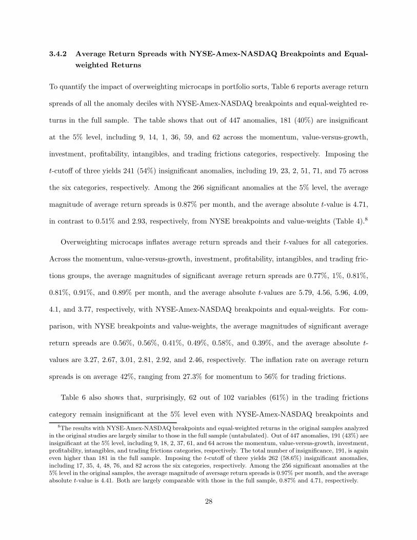
To quantify the impact of overweighting microcaps in portfolio sorts, Table 6 reports average return

spreads of all the anomaly deciles with NYSE-Amex-NASDAQ breakpoints and equal-weighted re-

turns in the full sample. The table shows that out of 447 anomalies, 181 (40%) are insignificant

at the 5% level, including 9, 14, 1, 36, 59, and 62 across the momentum, value-versus-growth,

investment, profitability, intangibles, and trading frictions categories, respectively. Imposing the

t-cutoff of three yields 241 (54%) insignificant anomalies, including 19, 23, 2, 51, 71, and 75 across

the six categories, respectively. Among the 266 significant anomalies at the 5% level, the average

magnitude of average return spreads is 0.87% per month, and the average absolute t-value is 4.71,

in contrast to 0.51% and 2.93, respectively, from NYSE breakpoints and value-weights (Table 4).8

Overweighting microcaps inflates average return spreads and their t-values for all categories.

Across the momentum, value-versus-growth, investment, profitability, intangibles, and trading fric-

tions groups, the average magnitudes of significant average return spreads are 0.77%, 1%, 0.81%,

0.81%, 0.91%, and 0.89% per month, and the average absolute t-values are 5.79, 4.56, 5.96, 4.09,

4.1, and 3.77, respectively, with NYSE-Amex-NASDAQ breakpoints and equal-weights. For com-

parison, with NYSE breakpoints and value-weights, the average magnitudes of significant average

return spreads are 0.56%, 0.56%, 0.41%, 0.49%, 0.58%, and 0.39%, and the average absolute t-

values are 3.27, 2.67, 3.01, 2.81, 2.92, and 2.46, respectively. The inflation rate on average return

spreads is on average 42%, ranging from 27.3% for momentum to 56% for trading frictions.

Table 6 also shows that, surprisingly, 62 out of 102 variables (61%) in the trading frictions

category remain insignificant at the 5% level even with NYSE-Amex-NASDAQ breakpoints and

8The results with NYSE-Amex-NASDAQ breakpoints and equal-weighted returns in the original samples analyzedin the original studies are largely similar to those in the full sample (untabulated). Out of 447 anomalies, 191 (43%) areinsignificant at the 5% level, including 9, 18, 2, 37, 61, and 64 across the momentum, value-versus-growth, investment,profitability, intangibles, and trading frictions categories, respectively. The total number of insignificance, 191, is againeven higher than 181 in the full sample. Imposing the t-cutoff of three yields 262 (58.6%) insignificant anomalies,including 17, 35, 4, 48, 76, and 82 across the six categories, respectively. Among the 256 significant anomalies at the5% level in the original samples, the average magnitude of aversage return spreads is 0.97% per month, and the averageabsolute t-value is 4.41. Both are largely comparable with those in the full sample, 0.87% and 4.71, respectively.

28

equal-weights. We interpret the evidence as indicating an excessive amount of flexibility with

cross-sectional regressions commonly adopted in the liquidity literature (Section 3.1.1).

Again, 15 out of 16 volatility measures produce economically small and statistically insignificant

average return spreads. Five measures even produce positive average return spreads, albeit all

insignificant, and 13 measures have absolute t-values below one. The evidence is even weaker than

that in Table 3 based on NYSE breakpoints and value-weights. In untabulated results, we show

that 9 out of 16 volatility measures generate significant average return spreads with NYSE-Amex-

NASDAQ breakpoints and value-weights. As such, the low volatility anomaly is extremely fragile.

The Acharya-Pedersen (2005) liquidity betas again fare poorly. All 15 variables from interacting

five beta measures with three horizons earn economically small and statistically insignificant average

return spreads. However, other liquidity measures perform well with NYSE-Amex-NASDAQ break-

points and equal-weights, including share turnover (Tur), dollar trading volume (Dtv), share price

(Pps), absolute return-to-volume (Ami), zero daily volume (Lm), and short-term reversal (Srev).

3.4.3 Portfolio Weights on Microcaps and Investment Capacity

Table 7 shows further why microcaps should be alleviated in any portfolio construction. Panel

A reports the average portfolio weights allocated to microcaps for the extreme deciles across the

six categories of anomalies. Our benchmark procedure with NYSE breakpoints and value-weights

assigns a modest amount of weights on microcaps, while the alternative procedure with NYSE-

Amex-NASDAQ breakpoints and equal-weights invests a disproportionately large amount. For

instance, in the momentum category, the low decile assigns on average 7.34% on microcaps under the

benchmark procedure, but 64.19% under the alternative. In the investment category, the high decile

assigns 5.69% on microcaps under the benchmark procedure, but 60.89% under the alternative.

In addition, the investment capacity on microcaps is limited. We measure a portfolio’s invest-

ment capacity as mini{Mei/wi}, in which i is the index of all the stocks in the portfolio, Mei is

stock i’s market equity, and wi is its weight in the portfolio. Mei/wi is the maximum amount that

29

the portfolio can invest in stock i by buying up all its shares, without considering the availability

of shares of other stocks in the portfolio. We need to take the minimum Mei/wi across the index

i because buying up any stock would exhaust the investment capacity of the portfolio.

For an equal-weighted portfolio, wi = 1/n, in which n is the number of stocks in the portfolio.

As such, the investment capacity equals mini{Mei/wi} = n × mini{Mei}. Intuitively, if an equal

amount of dollars is invested in each stock in the portfolio, its investment capacity is restricted by

the stock with the smallest market equity. For a value-weighted portfolio, wi = Mei/∑

iMei. The

investment capacity becomes mini{Mei/wi} = mini{∑

iMei} =∑

iMei, the total market equity of

all stocks in the portfolio, which is much higher than the investment capacity under equal-weights.

Panel B of Table 7 shows that the investment capacity with NYSE breakpoints and value-weights

is about several orders of magnitude larger than that with NYSE-Amex-NASDAQ breakpoints and

equal-weights. For example, in the momentum category, the investment capacity of the low decile is

on average 7.12% of the total market equity with our benchmark procedure, but only 0.016% with

the alternative construction. In the investment category, the investment capacity of the high decile

is on average 7.49% of the total market equity, but only 0.017% with the alternative procedure.

4 Explaining Significant Anomalies with the q-factor Model

In this section, we use the q-factor model to explain significant anomalies with NYSE breakpoints

and value-weighted returns in the full sample. We discuss the model’s performance in Section 4.1,

and highlight its weaknesses in Section 4.2. Appendix C details the q-factors construction, including

a new procedure that extends the sample of the q-factors backward from 1972 to 1967.

4.1 The q-factor Regressions

From January 1967 to December 2014, the size, investment, and Roe factors in the q-factor model

earn on average 0.32%, 0.43%, and 0.56% per month (t = 2.42, 5.08, and 5.24), respectively. The

investment and Roe factor premiums cannot be explained by the Carhart (1997) four-factor model,

30

with alphas of 0.29% (t = 4.57) and 0.51% (t = 5.58), or the Fama-French (2015) five-factor model,

with alphas of 0.12% (t = 3.35) and 0.45% (t = 5.6), respectively. (The data for the Carhart factors,

including the momentum factor, UMD, and the five factors are from Kenneth French’s Web site.)

UMD earns an average return of 0.67% (t = 3.66), but its q-factor alpha is only 0.11% (t = 0.43).

In the five-factor model, the average RMW and CMA returns are 0.27% (t = 2.58) and 0.34%

(t = 3.63), but their q-factor alphas are only 0.04% and 0.01% (t = 0.42 and 0.32), respectively.

Table 8 shows that across the 161 significant anomalies, the average magnitude of the high-

minus-low alphas is 0.26% per month, and the number of significant high-minus-low alphas is 46 at

the 5% level (11 with t ≥ 3). The mean absolute alpha is 0.12%, and the number of rejections by

the Gibbons, Ross, and Shanken (1989, GRS) test is 107 at the 5% level and 72 at the 1% level.

Columns 1–37 in Table 8 report the q-factor regressions for the 37 significant momentum anoma-

lies. For the high-minus-low deciles on prior 6-month returns (R6) at the 1-, 6-, and 12-month, the

q-factor alphas are −0.04%, 0.24%, and 0.16% per month (t = −0.1, 0.78, and 0.75), respectively.

The Roe factor is the main source of the model’s performance. In total 35 high-minus-low deciles

have positive Roe-factor loadings, and the two negative loadings are tiny and insignificant. The

average loading is 0.57. All but three of the positive loadings are significant, including 28 with

t-values above three. In particular, the high-minus-low R6 decile at the 6-month has an Roe-factor

loading of 0.99 (t = 5.33), and its investment-factor loading is tiny, −0.01 (t = −0.04).

Columns 38–68 in Table 8 show the q-factor regressions for the 31 significant value-versus-growth

anomalies. The high-minus-low book-to-market (Bm) decile has a q-factor alpha of 0.18% (t = 1.15).

The investment factor is the main source of the model’s performance. All 31 high-minus-low deciles

have investment-factor loadings that go in the right direction in explaining average returns. The

Roe-factor loadings often go in the wrong direction, and 18 are significant, but the investment-factor

loadings dominate the Roe-factor loadings. In particular, the high-minus-low Bm decile has an

investment-factor loadings of 1.33 (t = 3.09) relative to an Roe-factor loading of −0.55 (t = −6.64).

31

Columns 69–95 in Table 8 report the q-factor regressions for the 27 significant investment anoma-

lies. The high-minus-low decile on composite equity issuance (Cei) has a q-factor alpha of −0.24%

(t = −1.85). The investment factor is the main source of the model’s explanatory power. Most high-

minus-low deciles all have economically large and significantly negative loadings on the low-minus-

high investment factor. In contrast, the Roe-factor loadings have mixed signs. The Roe-factor

loadings can occasionally be significantly positive, going in the wrong direction, but are dominated

by the strong investment-factor loadings. The high-minus-low Cei decile has an investment-factor

loading of −1.04 (t = −13.74) relative to an Roe-factor loading of −0.12 (t = −1.57).

Columns 96–128 in Table 8 report the q-factor regressions for the 33 significant profitability

anomalies. At the 1-, 6-, and 12-month, the high-minus-low quarterly F-score (Fq) decile earns

q-factor alphas of 0.13%, 0.15%, and 0.07% (t = 0.58, 0.86, and 0.49), respectively. The Roe factor

is the main source of the model’s performance. All but one Roe-factor loadings are highly signif-

icant, with the t-value magnitudes above five, and the average magnitude of the loadings is 0.73.

For example, at the 1-, 6-, and 12-month, the high-minus-low Fq decile have Roe-factor loadings of

0.73, 0.67, and 0.65 (t = 6.97, 6.9, and 7.11), respectively. Their investment-factor loadings are also

significantly positive, but are dominated by the Roe-factor loadings. Finally, columns 129–154 in

Table 8 report the q-factor regressions for the 26 significant intangibles anomalies, and the remain-

ing columns report seven significant trading frictions anomalies. A combination of the investment-

and Roe-factor loadings helps explain the model’s performance.

4.2 The Weaknesses of the q-factor Model

In this subsection, we highlight the anomalies that the q-factor model cannot explain. We first

detail the individual q-anomalies, and then explore their potential commonality.

4.2.1 Individual q-anomalies

From Table 8, nine momentum anomalies have significant q-factor alphas, including two with t ≥ 3.

The high-minus-low deciles on abnormal returns around earnings announcements (Abr) at the 1-,

32

6-, and 12-month earn q-factor alphas of 0.66%, 0.27%, and 0.23% per month (t = 4.49, 2.41, and

2.65), respectively. Their Roe-factor loadings are economically weak, ranging only from 0.16 to

0.26, albeit significant. In addition, the high-minus-low decile on industry lead-lag effect in prior

returns (Ilr) has a q-alpha of 0.79% (t = 3.15) at the 1-month. The culprit is an extremely weak

Roe-factor loading, 0.08 (t = 0.59). Large q-factor alphas also show up in the high-minus-low deciles

on change in analysts’ forecasts (dEf), supplier industries momentum (Sim), customer momentum

(Cm), and customer industries momentum (Cim), all at the 1-month. Their q-factor alphas are

0.64%, 0.61%, 0.72%, and 0.64% (t = 2.81, 2.18, 2.75, and 2.29).

Six value-versus-growth anomalies have significant q-factor alphas, but none with t ≥ 3. At the

1-, 6-, and 12-month, the q-factor alphas of the high-minus-low cash flow-to-price (Cpq) deciles are

0.5%, 0.38%, and 0.22% per month (t = 2.27, 1.98, and 1.24), respectively. The strongly negative

Roe-factor loadings, which go in the wrong direction, hurt the q-factor model. At the 1-, 6-, and

12-month, these loadings are −0.61, −0.56, and −0.45 (t = −4.3, −4.7, and −4.16), despite their

strong investment-factor loadings of 0.99, 0.97, and 1.01 (t = 6.12, 6.74, and 7.57), respectively.

Seven investment anomalies have significant q-factor alphas, and three with t ≥ 3. The q-factor

model cannot explain the operating accruals (Oa) anomaly. The high-minus-low q-factor alpha is

−0.54% per month (t = −3.77). The investment-factor loadings is tiny, −0.02 (t = −0.23). In

contrast, the Roe-factor loading is large and significant, 0.26 (t = 4.13), which goes in the wrong

direction. The problem deepens with discretionary accruals (Dac), which purge the sales change

and property, plant, and equipment from Oa. The high-minus-low Dac decile has a q-factor alpha

of −0.64% (t = −4.37). Both investment- and Roe-factor loadings go in the wrong direction, 0.23

and 0.19 (t = 2.38 and 3.05), respectively. Three other accrual measures also cause problems for the

q-factor model, including net operating assets (Noa), change in net noncash working capital (dWc),

and change in net financial assets (dFin). The high-minus-low Noa, dWc, and dFin deciles have

q-factor alphas of −0.41%,−0.48%, and 0.44% (t = −2.24,−3.43, and 2.94), respectively. Their

investment-factor loadings are insufficient to bring the q-factor alphas to insignificance.

33

Nine profitability anomalies have significant q-factor alphas, including three with t ≥ 3. The

high-minus-low cash-based operating profits-to-assets (Cop) decile has a q-factor alpha of 0.69%

per month (t = 4.77). Scaling with lagged assets (Cla) raises the q-factor alpha to 0.74% (t = 4.89).

Monthly sorts on Cla yield q-factor alphas of 0.43%, 0.4%, and 0.46% (t = 2.69, 2.82, and 3.56)

at the 1-, 6-, and 12-month, respectively. The size-factor loadings all go in the wrong direction

in explaining average returns, and the investment-factor loadings too, but weakly. The Roe-factor

loadings, all of which are significantly positive, are not large enough to undo the damage.

The q-factor model leaves 11 intangible anomalies significant, including four with t ≥ 3. The

q-factor model cannot capture the R&D-to-market (Rdm) anomaly. In annual sorts, the high-

minus-low decile earns a q-factor alpha of 0.7% per month (t = 2.89). In monthly sorts at the

1-, 6-, and 12-month, the high-minus-low deciles have q-factor alphas of 1.47%, 0.97%, and 0.8%

(t = 2.97, 2.73, and 2.8), respectively. The investment-factor loadings, most of which are signifi-

cant, go in the right direction in explaining average returns. However, the Roe-factor loadings, all

of which are economically large and statistically significant, go in the wrong direction.

The q-factor model also fails to capture the Heston-Sadka (2008) seasonality anomalies. At the

beginning of each month t, we split stocks into deciles based on various measures of past perfor-

mance, including returns in month t−12 (R1a), average returns across months t−24, t−36, t−48,

and t−60 (R[2,5]a ), average returns across months t−72, t−84, t−96, t−108, and t−120 (R

[6,10]a ),

average returns across months t−132, t−144, t−156, t−168, and t−180 (R[11,15]a ), and average returns

across months t−192, t−204, t−216, t−228, and t−240 (R[16,20]a ). Monthly decile returns are calcu-

lated for the current month t, and the deciles are rebalanced at the beginning of month t+1. The

q-factor alphas of the high-minus-low deciles on R1a, R

[2,5]a , R

[6,10]a , R

[11,15]a , and R

[16,20]a are 0.55%,

0.81%, 1.13%, 0.65%, and 0.64% per month (t = 2.48, 3.9, 4.88, 3.6, and 3.14), respectively. The

investment- and Roe-factor loadings are mostly economically small and statistically insignificant.

Finally, four friction anomalies are significant in the q-factor model, including one with t ≥ 3.

34

The high-minus-low deciles on total skewness (Ts), idiosyncratic skewness per the three-factor

model (Isff), and idiosyncratic skewness per the q-factor model (Isq), have q-factor alphas all

around 0.31% per month, with t-values from 2.64 to 3.01. Both q-factor loadings are close to zero.

4.2.2 Commonality in q-anomalies

To explore the potential commonality among the 46 significant q-anomalies, we calculate their pair-

wise cross-sectional rank correlations based on each anomaly variable’s NYSE percentile rankings.

Panel A of Table 9 shows average within-category and average cross-category rank correlations.

Our categorization of anomalies based on a priori economic arguments is consistent with statisti-

cal clustering. In particular, average within-category correlations are generally large, but average

cross-category correlations are close to zero. Panel B digs deeper by reporting average within-

category correlations for each individual q-anomaly. Except for intangibles, anomalies within each

category tend to be positively correlated. With a few exceptions such as Ile1, dRoe1, and Ami12,

the positive correlations tend to be high. For intangibles, however, the Heston-Sadka (2008) sea-

sonality variables have correlations close to zero, both among themselves and with other intangible

variables. As a result, the average within-category correlation for intangibles is only 0.07.9

To evaluate the overall economic significance of the q-anomalies, we follow Stambaugh and Yu

(2016) to form a composite measure for each category of q-anomalies by equal-weighting a stock’s

NYSE percentile rankings across the q-anomalies within the category. Some anomalies within a

given category predict returns with opposite signs. We adjust the signs of all anomalies within the

category to ensure a universally positive sign in forecasting returns. Also, some anomalies have

different sample starting points. We start with January 1967, and always use all available anomaly

variables at a given point of time in constructing a composite measure. We form deciles on the

composite measure for each category as well as by combining all 46 q-anomalies.

9We have experimented with principle component analysis for the 46 q-anomalies. Consistent with the clusteranalysis based on rank correlations, the first six principle components capture 15.3%, 12.9%, 7.8%, 5.4%, 4.9%,and 4.6% (in total 51%) of the time series variation of the 46 high-minus-low returns, respectively. As such, theq-anomalies tend to be relatively diffused, especially with the Heston-Sadka (2008) seasonality variables in the mix.

35

The q-factor model is far from perfect. The average return spreads on the composite measures

for the momentum, value-versus-growth, investment, profitability, intangibles, and frictions cate-

gories are 1.1%, 0.6%, 0.6%, 0.71%, 1.08%, and 0.14% per month (t = 5.72, 2.94, 4.27, 4.17, 6.92,

and 0.92), and their q-factor alphas 0.86%, 0.41%, 0.69%, 0.58%, 0.85%, and 0.16% (t =

3.67, 2.09, 4.28, 4.11, 5.08, and 1.52), respectively. Curiously, combining the four friction variables

destroys their forecasting power. Digging deeper, we find that the average return spreads based

on their individual sorts shrink quickly once calculated as the differences between deciles two and

nine (untabulated). Taking the average across the rankings ends up adding noise into the extreme

deciles. In contrast, the low within-category correlations among intangibles imply independent

forecasting power for individual intangible anomalies, and taking the average rankings aggregates

over the signals to produce a high average return spread. Finally, combining all 46 q-anomalies

leads to an average return spread of 1.66% (t = 10.28), and the q-factor alpha is 1.4% (t = 7.48).

5 Summary and Implications

We have attempted to replicate the bulk of the published anomalies literature in finance and

accounting by compiling a largest-to-date data library that consists of 447 anomalies. After we

control for microcaps with NYSE breakpoints and value-weighted returns, 286 anomalies (64%)

are insignificant at the conventional 5% level. Imposing the t-value cutoff of three increases the

number of insignificance further to 380 (85%). In the trading frictions category that contains mostly

liquidity variables, 95 out of 102 (93%) are insignificant at the 5% level. The distress anomaly is also

virtually nonexistent in our replication. Even for significant anomalies, such as price momentum

and operating accruals, their magnitudes are often much lower than originally reported. Finally, out

of the 161 significant anomalies, the q-factor model leaves 115 alphas insignificant (150 with t < 3).

In totality, our evidence suggests that capital markets are more efficient than previously reported.

How should we move forward in the anomalies literature? As noted, Ioannidis (2005) develops

a theoretical model which predicts that results in a scientific field are more likely to be false when

36

the studies use smaller samples, when the effects are smaller in magnitude, when there are many

empirical but fewer theoretically predicted relations, when authors have greater flexibility in de-

signs, variable definitions, and empirical specifications, when there exist greater financial and other

interest and publication biases, and when more independent teams are involved in a given field.

We apply this conceptual framework to discuss implications of our replication on future work.

5.1 Taking the Con out of Anomalies

First, on the flexibility in test designs, variable definitions, and empirical specifications, our replica-

tion indicates widespread p-hacking, mainly by overweighting microcaps. Many studies overweight

microcaps via NYSE-Amex-NASDAQ (not NYSE) breakpoints, often also with equal-weights, in

portfolio sorts. Hundreds of studies use Fama-MacBeth (1973) cross-sectional regressions of future

returns on anomaly variables, which assign even higher weights to microcaps than equal-weights

in sorts. As such, most published anomaly profits are greatly exaggerated. We recommend NYSE

breakpoints and value-weights in sorts as the benchmark method, as evident in the construction

of all common factors. While alternative specifications are not technically wrong, results from the

benchmark method should always be presented in the spirit of Leamer (1983).

Second, on the sample size, most studies use the U.S.-centric CRSP-Compustat data. Karolyi

(2016) shows that only 16% of all empirical studies in the top four finance journals examine non-

U.S. markets, a percentage that is well below measures of their economic importance in the world

economy. We agree with Karolyi that large-scale investigations of the global data available in Datas-

tream and Worldscope are likely to improve the quality of the anomalies literature. These out-of-

sample investigations are especially valuable for anomalies that are highly significant, but seem to

lack a priori economic underpinnings, such as the Heston-Sadka (2008) seasonality anomalies.

Third, authors, referees, and editors should be keenly aware of the complex agency problem

that can arise from financial conflicts of interest and publication biases. Referees can be more

open to papers that take care in developing well grounded economic hypotheses, even though their

37

empirical findings might not be (that) significant. With this publication bias alleviated, authors

would most likely have fewer incentives to engage in p-hacking. When working with junior coau-

thors, senior academics should be alert to potential conflicts of interest in that junior coauthors

are more likely to p-hack, perhaps due to tenure pressure (Brodeur, Le, Sangnier, and Zylberberg

2016). Empirical results can be very sensitive to the adopted specifications, and those from the

most standard specifications are the most persuasive.

5.2 Taking Economic Theory Seriously

Perhaps most important, the credibility of the anomalies literature can improve via a closer connec-

tion with economic theory. Ioannidis (2005) emphasizes the importance of theoretical predictions,

specifically, by raising the ratio of ex ante true relations to false relations tested in a field, Ri, in

equations (1) and (2). Harvey, Liu, and Zhu (2016, p. 7) also write: “A factor derived from a theory

should have a lower hurdle than a factor discovered from a purely empirical exercise. Economic

theories are based on a few economic principles and, as a result, there is less room for data mining.”

In response to the theoretical vacuum left by the CAPM in the early 1990s, Fama and French

(1993) form their three-factor model by augmenting the market factor with two characteristics-based

factors on size and book-to-market. However, the empirical nature of these factors leaves the three-

factor model vulnerable to the data mining critique. In contrast, the q-factor model is economically

motivated from the first principle of real investment for individual firms. Our extensive evidence

on the relative successes and weaknesses of the q-factor model suggests several fruitful directions

for future research, all of which involve rich interactions between theory and empirics.

First, despite their economic motivation and t > 5 in our sample, the investment and Roe

factors in the q-factor model are not entirely immune to p-hacking. For example, Linnainmaa and

Roberts (2016) show that the Fama-French (2015) operating profitability premium is insignificant

in the pre-Compustat sample (the Roe premium is not examined, probably due to the lack of quar-

terly earnings data). An effective way to address the lingering data mining concern is to examine

38

global financial data, following Karolyi’s (2016) advice. Another way to proceed is to examine

alternative asset classes, such as corporate bonds, sovereign bonds, equity derivatives, real estate,

private equity, and currencies. Are investment and Roe priced in the returns of these alternative

assets? How does the q-factor model in these markets perform relative to their benchmark models?

Second, while the q-factor model is motivated from the first principle of real investment, the

connection between theory and empirics can be strengthened. A theoretical literature based on

real options and neoclassical investment models has been developing since the late 1990s, initially

aiming at explaining the value premium (Berk, Green, and Naik 1999; Carlson, Fisher, and Gi-

ammarino 2004; Zhang 2005). More recently, the literature has focused on explaining the failure of

the CAPM in capturing the value premium (Kogan and Papanikolaou 2013), as well as explaining

momentum and value simultaneously (Li 2016). Can the investment and Roe premiums be ex-

plained simultaneously in a quantitative investment model? What drives the comovement behind

the investment and Roe factors, the cross-sectional heterogeneity in investment and Roe, as well as

the failure of the CAPM in explaining the two premiums? What explains the broad explanatory

power of the q-factor model in the cross section, including anomalies formed on variables that are

not directly related to investment and profitability? These theoretical questions are important.

After all, Stambaugh and Yu (2016) interpret their two factors, despite being closely related to the

q-factors, as driven by mispricing. When more empirical work is futile, careful theorizing can shed

light on the risk-versus-mispricing debate, as in the case of the value premium.

Third, for the 46 q-anomalies, we suspect that the q-factor model’s weaknesses might be at-

tributed to a missing expected growth factor. In the multiperiod investment model, expected

returns vary cross-sectionally, depending on investment, Roe, and expected investment growth.

Prior work shows that the expected growth plays an important role in explaining earnings and

price momentum as well as their short-lived dynamics (Liu, Whited, and Zhang 2009; Liu and

Zhang 2014). George, Hwang, and Li (2016) show that the 52-week high variable better predicts

future investment growth than Roe. However, concerned with the lack of a reliable expected growth

39

proxy (Chan, Karceski, and Lakonishok 2003), Hou, Xue, and Zhang (2015) opt to drop the ex-

pected growth factor, and use only the two-period investment model to motivate the investment

and Roe factors. This omission likely matters because some of the q-anomaly variables might be

better predictors of future growth rates than Roe. Examples include abnormal returns around

earnings announcements, industry lead-lag in prior returns, four-quarter-change in Roe, cash-based

operating profitability, and R&D-to-market. In particular, R&D is expensed in the data. As such,

R&D expenses depress current Roe, but raise future Roe, and consequently, the expected growth.

Future work can explore the role of the expected growth in explaining the q-anomalies.

Finally, we emphasize that theories should be developed on the economic foundation of first

principles, before doing the empirical work, to guard against HARKing (hypothesizing after the

results are known) (Kerr 1998). Kerr defines HARKing as presenting a post hoc hypothesis based

on or informed by one’s evidence in the introduction of a research article as if it were an a priori

hypothesis. Kerr argues that HARKing is hazardous for scientific progress: (i) it translates false

positive findings into theories; (ii) it promotes theories that are more context-specific and ad hoc,

less useful, and less refutable; (iii) it breeds statistical abuses and questionable practices in ethically

ambiguous areas; and (iv) it discourages the identification of more general theories and plausible

alternative hypotheses. In contrast, theories based on first principles are more general, less ad hoc,

and more refutable, and can serve as an effective antidote of HARKing.

40

References

Abarbanell, Jeffery S., and Brian J. Bushee, 1998, Abnormal returns to a fundamental analysisstrategy, The Accounting Review 73, 19–45.

Acharya, Viral V., and Lasse H. Pedersen, 2005, Asset pricing with liquidity risk, Journal of

Financial Economics 77, 375–410.

Adrian, Tobias, Erkko Etula, and Tyler Muir, 2014, Financial intermediaries and the cross-sectionof asset returns, Journal of Finance 69, 2557–2596.

Ali, Ashiq, Lee-Seok Hwang, and Mark A. Trombley, 2003, Arbitrage risk and the book-to-marketanomaly, Journal of Financial Economics 69, 355–373.

American Statistical Association, 2016, ASA statement on statistical significance and p-values,The American Statistician 70, 131–133.

Amihud, Yakov, 2002, Illiquidity and stock returns: Cross-section and time series evidence,Journal of Financial Markets 5, 31–56.

Anderson, Christopher W., and Luis Garcia-Feijoo, 2006, Empirical evidence on capitalinvestment, growth options, and security returns, Journal of Finance 61, 171–194.

Anderson, Evan W., Eric Ghysels, and Jennifer L. Juergens, 2005, Do heterogeneous beliefs matterfor asset pricing? Review of Financial Studies 18, 875–924.

Ang, Andrew, 2014, Asset Management: A Systematic Approach to Factor Investing, OxfordUniversity Press.

Ang, Andrew, Joseph Chen, and Yuhang Xing, 2006, Downside risk, Review of Financial Studies

19, 1191–1239.

Ang, Andrew, Robert J. Hodrick, Yuhang Xing, and Xiaoyan Zhang, 2006, The cross-section ofvolatility and expected returns, Journal of Finance 61, 259–299.

Asness, Clifford, and Andrea Frazzini, 2013, The devil in HML’s details, Journal of Portfolio

Management 39, 49–68.

Asparouhova, Elena, Hendrik Bessembinder, and Ivalina Kalcheva, 2013, Noisy prices andinference regarding returns, Journal of Finance 68, 665–714.

Avramov, Doron, Tarun Chordia, Gergana Jostova, and Alexander Philipov, 2009, Credit ratingsand the cross-section of stock returns, Journal of Financial Markets 12, 469–499.

Baker, Monya, 2016, Is there a reproducibility crisis? Nature 533, 452–454.

Balakrishnan, Karthik, Eli Bartov, and Lucile Faurel, 2010, Post loss/profit announcement drift,Journal of Accounting and Economics 50, 20–41.

Bali, Turan G., and Nusret Cakici, 2008, Idiosyncratic volatility and the cross section of expectedreturns, Journal of Financial and Quantitative Analysis 43, 29-58.

Bali, Turan G., Nusret Cakici, and Robert F. Whitelaw, 2011, Maxing out: Stocks as lotteriesand the cross-section of expected returns, Journal of Financial Economics 99, 427–446.

41

Bali, Turan G., Robert F. Engle, and Scott Murray, 2016, Empirical asset pricing: The Cross

Section of Stock Returns Hoboken: Wiley.

Ball, Ray, and Philip Brown, 1968, An empirical evaluation of accounting income numbers, Journalof Accounting Research 6, 159-178.

Ball, Ray, Joseph Gerakos, Juhani Linnainmaa, and Valeri Nikolaev, 2015, Deflating profitability,Journal of Financial Economics 117, 225–248.

Ball, Ray, Joseph Gerakos, Juhani Linnainmaa, and Valeri Nikolaev, 2016, Accruals, cashflows, and operating profitability in the cross section of stock returns, Journal of FinancialEconomics 121, 28–45.

Banz, Rolf W., 1981, The relationship between return and market value of common stocks, Journalof Financial Economics 9, 3–18.

Basu, Sanjoy, 1983, The relationship between earnings yield, market value, and return for NYSEcommon stocks: Further evidence, Journal of Financial Economics 12, 129–156.

Barbee, William C., Jr., Sandip Mukherji, and Gary A. Raines, 1996, Do sales-price and debt-equity explain stock returns better than book-market and firm size? Financial Analysts

Journal 52, 56-60.

Barth, Mary E., John A. Elliott, and Mark W. Finn, 1999, Market rewards associated withpatterns of increasing earnings, Journal of Accounting Research 37, 387–413.

Beaver, William, Maureen McNichols, and Richard Price, 2007, Delisting returns and their effecton accounting-based market anomalies, Journal of Accounting and Economics 43, 341–368.

Begely, C. Glenn, and Lee M. Ellis, 2012, Drug development: Raise standards for preclinicalcancer research, Nature 483, 531–533.

Belo, Frederico, and Xiaoji Lin, 2011, The inventory growth spread, Review of Financial Studies

25, 278–313.

Belo, Frederico, Xiaoji Lin, and Santiago Bazdresch, 2014, Labor hiring, investment, and stockreturn predictability in the cross section, Journal of Political Economy 122, 129–177.

Belo, Frederico, Xiaoji Lin, and Maria Ana Vitorino, 2014, Brand capital and firm value, Reviewof Economic Dynamics 17, 150–169.

Berk, Jonathan B., Richard C. Green, and Vasant Naik, 1999, Optimal investment, growth options,and security returns, Journal of Finance 54, 1153–1607.

Bernard, Victor L., and Jacob K. Thomas, 1989, Post-earnings-announcement drift: Delayed priceresponse or risk premium? Journal of Accounting Research Supplement 27, 1-48.

Berry, James, Lucas C. Coffman, Douglas Hanley, Rania Gihleb, and Alistair J. Wilson, 2017,Assessing the rate of replication in economics, American Economic Review 107, 27–31.

Bhandari, Laxmi Chand, 1988, Debt/equity ratio and expected common stock returns: Empiricalevidence, Journal of Finance 43, 507–528.

42

Black, Fischer, Michael C. Jensen, and Myron Scholes, 1972, The Capital Asset Pricing Model:Some empirical tests, in Studies in the Theory of Capital Markets, edited by Michael C.Jensen, New York: Praeger, 79–121.

Blitz, David, Joop Huij, and Martin Martens, 2011, Residual momentum, Journal of Empirical

Finance 18, 506–521.

Blume, Marshall E., and Robert F. Stambaugh, 1983, Biases in computed returns: An applicationto the size effect, Journal of Financial Economics 12, 387–404.

Boudoukh, Jacob, Roni Michaely, Matthew Richardson, and Michael R. Roberts, 2007, On theimportance of measuring payout yield: Implications for empirical asset pricing, Journal ofFinance 62, 877–915.

Bradshaw, Mark T., Scott A. Richardson, and Richard G. Sloan, 2006, The relation betweencorporate financing activities, analysts’ forecasts and stock returns, Journal of Accountingand Economics 42, 53–85.

Breeden, Douglas T., 1979, An intertemporal asset pricing model with stochastic consumptionand investment opportunities, Journal of Financial Economics 7, 265–296.

Brennan, Michael J., Tarun Chordia, and Avanidhar Subrahmanyam, 1998, Alternative factorspecifications, security characteristics, and the cross-section of expected stock returns, Journalof Financial Economics 49, 345–373.

Brodeur, Abel, Mattias Le, Marc Sangnier, and Yanos Zylberberg, 2016, Star wars: The empiricsstrike back, American Economic Journal: Applied Economics 8, 1–32.

Bruns, Stephan B., and John P. A. Ioannidis, 2016, P-curve and p-hacking in observationalresearch, PLoS One 11: e0149144.

Camerer, Colin F., Anna Dreber, Eskil Forsell, Teck-Hua Ho, Jurgen Huber, Magnus Johannesson,Michael Kirchler, et al., 2016. Evaluating replicability of laboratory experiments in economics,Science 351, 1433-1436.

Campbell, John Y., Jens Hilscher, and Jan Szilagyi, 2008, In search of distress risk, Journal ofFinance 63, 2899–2939.

Card, David E., and Alan B. Krueger, 1995, Time-series minimum-wage studies: A meta-analysis,American Economic Review 85, 238–243.

Carhart, Mark M. 1997, On persistence in mutual fund performance, Journal of Finance 52,57–82.

Carlson, Murray, Adlai Fisher, and Ron Giammarino, 2004, Corporate investment and asset pricedynamics: Implications for the cross section of returns, Journal of Finance 59, 2577–2603.

Chan, Louis K. C., Jason Karceski, and Josef Lakonishok, 2003, The level and persistence ofgrowth rates, Journal of Finance 58, 643–684.

Chan, Louis K. C., Narasimhan Jegadeesh, and Josef Lakonishok, 1996, Momentum strategies,Journal of Finance 51, 1681–1713.

43

Chan, Louis K. C., Josef Lakonishok, and Theodore Sougiannis, 2001, The stock market valuationof research and development expenditures, Journal of Finance 56, 2431–2456.

Chang, Andrew C., and Phillip Li, 2005, Is economics research replicable? Sixty published papersfrom thirteen journals say “usually not.” forthcoming, Critical Finance Review.

Chen, Shuping, Mark L. DeFond, and Chul W. Park, 2002, Voluntary disclosure of balance sheetinformation in quarterly earnings announcements, Journal of Accounting and Economics 33,229–251.

Christensen, Garret S., and Edward Miguel, 2016, Transparency, reproducibility, and thecredibility of economic research, NBER working paper 22989.

Chordia, Tarun, Avanidhar Subrahmanyam, and V. Ravi Anshuman, 2001, Trading activity andexpected stock returns, Journal of Financial Economics 59, 3–32.

Clemens, Michael A., 2017, The meaning of failed replications: A review and proposal, Journalof Economic Surveys 31, 326–342.

Cohen, Lauren, and Andrea Frazzini, 2008, Economic links and predictable returns, Journal ofFinance 63, 1977–2011.

Cohen, Lauren, and Dong Lou, 2012, Complicated firms, Journal of Financial Economics 104,383–400.

Conrad, Jennifer, Michael Cooper, and Gautam Kaul, 2003, Value versus glamour, Journal ofFinance 58, 1969–1995.

Cooper, Michael J., Huseyin Gulen, and Michael J. Schill, 2008, Asset growth and the cross-sectionof stock returns, Journal of Finance 63, 1609–1652.

Core, John E., Wayne R. Guay, and Tjomme O. Rusticus, 2006, Does weak governance cause weakstock returns? An examination of firm operating performance and investors’ expectations,Journal of Finance 61, 655–687.

Core, John E., Wayne R. Guay, and Rodrigo Verdi, 2008, Is accruals quality a priced risk factor?Journal of Accounting and Economics 46, 2–22.

Corwin, Shane A., and Paul Schultz, 2012, A simple way to estimate bid-ask spreads from dailyhigh and low prices, Journal of Finance 67, 719–759.

Coy, Peter, 2017, Lies, damn lies, and financial statistics, BloombergBusinessweek.

Da, Zhi, and Mitch Warachka, 2011, The disparity between long-term and short-term forecastedearnings growth, Journal of Financial Economics 100, 424–442.

Daniel, Kent D. and Sheridan Titman, 2006, Market reactions to tangible and intangibleinformation, Journal of Finance 61, 1605–1643.

Datar, Vinay T., Narayan Y. Naik, and Robert Radcliffe, 1998, Liquidity and stock returns: Analternative test, Journal of Financial Markets 1, 203–219.

44

Davis, James L., Eugene F. Fama, and Kenneth R. French, 2000, Characteristics, covariances,and average returns: 1929 to 1997, Journal of Finance 55, 389–406.

De Bondt, Werner F. M., and Richard Thaler, 1985, Does the stock market overreact? Journal of

Finance 40, 793–805.

Dechow, Patricia M., Richard G. Sloan, and Mark T. Soliman, 2004, Implied equity duration: Anew measure of equity risk, Review of Accounting Studies 9, 197–228.

De Long, J. Bradford, and Kevin Lang, 1992, Are all economic hypotheses false? Journal of

Political Economy 100, 1257–1272.

Desai, Hemang, Shivaram Rajgopal, and Mohan Venkatachalam, 2004, Value-glamour andaccruals mispricing: One anomaly or two? The Accounting Review 79, 355–385.

Dewald, William G., Jerry G. Thursby, and Richard G. Anderson, 1986, Replication in empiricaleconomics: The Journal of Money, Credit, and Banking project, American Economic Review

76, 587–630.

Dichev, Ilia, 1998, Is the risk of bankruptcy a systematic risk? Journal of Finance 53, 1141–1148.

Diether, Karl B., Christopher J. Malloy, and Anna Scherbina, 2002, Differences of opinion andthe cross section of stock returns, Journal of Finance 57, 2113–2141.

Dimson, Elroy, 1979, Risk management when shares are subject to infrequent trading, Journal ofFinancial Economics 7, 197–226.

Doidge, Craig, G. Andrew Karolyi, and Rene M. Stulz, 2013, The U.S. left behind? Financialglobalization and the rise of IPOs outside the U.S., Journal of Financial Economics 110,546–573.

Doidge, Craig, G. Andrew Karolyi, and Rene M. Stulz, 2017, The U.S. listing gap, Journal ofFinancial Economics 123, 464–487.

Duvendack, Maren, Richard Palmer-Jones, and W. Robert Reed, 2017, What is meant by“replication” and why does it encounter resistance in economics? American Economic Review

107, 46–51.

Easton, Peter D., and Mark E. Zmijewski, 1993, SEC form 10K/10Q reports and annual reportsto shareholders: Reporting lags and squared market model prediction errors, Journal of

Accounting Research 31, 113–129.

Eisfeldt, Andrea L., and Dimitris Papanikolaou, 2013, Organizational capital and the cross-sectionof expected returns, Journal of Finance 68, 1365–1406.

Elgers, Pieter T., May H. Lo, and Ray J. Pfeiffer, Jr., 2001, Delayed security price adjustmentsto financial analysts’ forecasts of annual earnings, The Accounting Review 76, 613–632.

Elton, Edwin J., 1999, Expected return, realized return, and asset pricing tests, Journal of Finance54, 1199-220.

45

Fairfield, Patricia M., J. Scott Whisenant, and Teri Lombardi Yohn, 2003, Accrued earnings andgrowth: Implications for future profitability and market mispricing, The Accounting Review

78, 353–371.

Fama, Eugene F., 1976, Foundations of Finance, New York: Basic Books, Publishers.

Fama, Eugene F., 1998, Market efficiency, long-term returns, and behavioral finance, Journal ofFinancial Economics 49, 283–306.

Fama, Eugene F., and Kenneth R. French, 1992, The cross-section of expected stock returns,Journal of Finance 47, 427-465.

Fama, Eugene F., and Kenneth R. French, 1993, Common risk factors in the returns on stocksand bonds, Journal of Financial Economics 33, 3–56.

Fama, Eugene F., and Kenneth R. French, 1996, Multifactor explanation of asset pricinganomalies, Journal of Finance 51, 55–84.

Fama, Eugene F., and Kenneth R. French, 1997, Industry costs of equity, Journal of FinancialEconomics 43, 153-93.

Fama, Eugene F., and Kenneth R. French, 2006, Profitability, investment, and average returns,Journal of Financial Economics 82, 491–518.

Fama, Eugene F., and Kenneth R. French, 2008, Dissecting anomalies, Journal of Finance 63,1653–1678.

Fama, Eugene F., and Kenneth R. French, 2015, A five-factor asset pricing model, Journal ofFinancial Economics 116, 1–22.

Fama, Eugene F., and James D. MacBeth, 1973, Risk return, and equilibrium: Empirical tests,Journal of Political Economy 81, 607–636.

Fanelli, Daniele, 2010, “Positive” results increase down the hierarchy of the sciences, PLoS One

5, e10068.

Foster, George, Chris Olsen, and Terry Shevlin, 1984, Earnings releases, anomalies, and thebehavior of security returns, The Accounting Review 59, 574–603.

Francis, Jennifer, Ryan LaFond, Per M. Olsson, and Katherine Schipper, 2004, Cost of equity andearnings attributes, The Accounting Review 79, 967–1010.

Francis, Jennifer, Ryan LaFond, Per M. Olsson, and Katherine Schipper, 2005, The market priceof accruals quality, Journal of Accounting and Economics 39, 295–327.

Franco, Annie, Neil Malhotra, and Gabor Simonovits, 2014, Publication bias in the social sciences:Unlocking the file drawer, Science 345, 1502–1505.

Frankel, Richard, and Charles M. C. Lee, 1998, Accounting valuation, market expectation, andcross-sectional stock returns, Journal of Accounting and Economics 25, 283–319.

Franzoni, Francesco, and Jose M. Marin, 2006, Pension plan funding and stock market efficiency,Journal of Finance 61, 921–956.

46

Frazzini, Andrea, and Lasse Heje Pedersen, 2014, Betting against beta, Journal of Financial

Economics 111, 1–25.

Freedman, Leonard P., Iain M. Cockburn, and Timothy S. Simcoe, 2015, The economics ofreproducibility in preclinical research, PLoS Biology 13: e1002165.

Gao, Xiaohui, Jay R. Ritter, and Zhongyan Zhu, 2013, Where have all the IPOs gone? Journal

of Financial and Quantitative Analysis 48, 1663–1692.

George, Thomas J., and Chuan-Yang Hwang, 2004, The 52-week high and momentum investing,Journal of Finance 58, 2145–2176.

Geroge, Thomas J., Chuan-Yang Hwang, and Yuan Li, 2016, The 52-week high, q theory, and thecross-section of stock returns, forthcoming, Journal of Financial Economics.

Gibbons, Michael R., Stephen A. Ross, and Jay Shanken, 1989, A test of the efficiency of a givenportfolio, Econometrica 57, 1121–1152.

Gompers, Paul, Joy Ishii, and Andrew Metrick, 2001, Corporate governance and equity prices,Quarterly Journal of Economics 118, 107–155.

Green, Jeremiah, John R. M. Hand, and X. Frank Zhang, 2013, The supraview of return predictivesignals, Review of Accounting Studies 18, 692–730.

Green, Jeremiah, John R. M. Hand, and X. Frank Zhang, 2016, The characteristics that provideindependent information about average U.S. monthly stock returns, working paper, YaleUniversity.

Hafzalla, Nader, Russell Lundholm, and E. Matthew Van Winkle, 2011, Percent accruals, TheAccounting Review 86, 209–236.

Hahn, Jaehoon, and Hangyong Lee, 2009, Financial constraints, debt capacity, and the cross-section of stock returns, Journal of Finance 64, 891–921.

Hamermesh, Daniel S., 2007, Viewpoint: Replication in economics, Canadian Journal of

Economics 40, 715–733.

Hamermesh, Daniel S., 2017, Replication in labor economics: Evidence from data and what itsuggests, American Economic Review 107, 37–40.

Han, Yufeng, and David A. Lesmond, 2011, Liquidity biases and the pricing of cross-sectionalidiosyncratic volatility, Review of Financial Studies 24, 1590–1629.

Harvey, Campbell R., 2017, Presidential address: The scientific outlook in financial economics,forthcoming, Journal of Finance.

Harvey, Campbell R., and Akhtar Siddique, 2000, Conditional skewness in asset pricing tests,Journal of Finance 55, 1263–1295.

Harvey, Campbell R., Yan Liu, and Heqing Zhu, 2016, ...and the cross-section of expected returns,Review of Financial Studies 29, 5–68.

47

Haugen, Robert A., and Nardin L. Baker, 1996, Commonality in the determinants of expectedstock returns, Journal of Financial Economics 41, 401-439.

Hawkins, Eugene H., Stanley C. Chamberlin, and Wayne E. Daniel, 1984, Earnings expectationsand security prices, Financial Analysts Journal 40, 24–38.

Heston Steven L., and Ronnie Sadka, 2008, Seasonality in the cross-section of stock returns,Journal of Financial Economics 87, 418–445.

Hirshleifer, David, Kewei Hou, Siew Hong Teoh, and Yinglei Zhang, 2004, Do investors overvaluefirms with bloated balance sheets? Journal of Accounting and Economics 38, 297–331.

Hirshleifer, David, Po-Hsuan Hsu, and Dongmei Li, 2013, Innovation efficiency and stock returns,Journal of Financial Economics 107, 632–654.

Hou, Kewei, 2007, Industry information diffusion and the lead-lag effect in stock returns, Reviewof Financial Studies 20, 1113–1138.

Hou, Kewei, and Roger K. Loh, 2015, Have we solved the idiosyncratic volatility puzzle? Journal

of Financial Economics 121, 167–194.

Hou, Kewei, and Tobias J. Moskowitz, 2005, Market frictions, price delay, and the cross-sectionof expected returns, Review of Financial Studies 18, 981–1020.

Hou, Kewei, and David T. Robinson, 2006, Industry concentration and average stock returns,Journal of Finance 61, 1927–1956.

Hou, Kewei, Chen Xue, and Lu Zhang, 2015, Digesting anomalies: An investment approach,Review of Financial Studies 28, 650–705.

Hribar, Paul, and Daniel W. Collins, 2002, Errors in estimating accruals: Implications for empiricalresearch, Journal of Accounting Research 40, 105–134.

Huang, Alan Guoming, 2009, The cross section of cashflow volatility and expected stock returns,Journal of Empirical Finance 16, 409–429.

Hunter, John E., 2001, The desperate need for replication, Journal of Consumer Reearch 28,149–158.

Ioannidis, John P. A., 2005, Why most published research findings are false, PLoS Med 2: e124.

Ioannidis, John P. A., 2012, Why science is not necessarily self-correcting, Perspectives on

Psychological Science 7, 645–654.

Ioannidis, John P. A., Tom D. Stanley, and Hristos Doucouliagos, 2015, The power of bias ineconomics research, forthcoming, Economic Journal.

Jagannathan, Ravi, and Yong Wang, 2007, Lazy investors, discretionary consumption, and thecross-section of stock returns, Journal of Finance 62, 1623–1661.

Jegadeesh, Narasimhan, 1990, Evidence of predictable behavior of security returns, Journal ofFinance 45, 881–898.

48

Jegadeesh, Narasimhan and Sheridan Titman, 1993, Returns to buying winners and selling losers:Implications for stock market efficiency, Journal of Finance 48, 65–91.

Jegadeesh, Narasimhan, and Joshua Livnat, 2006, Revenue surprises and stock returns, Journalof Accounting and Economics 41, 147–171.

Jiang, Guohua, Charles M. C. Lee, and Yi Zhang, 2005, Information uncertainty and expectedreturns, Review of Accounting Studies 10, 185–221.

John, Leslie K., George Loewenstein, and Drazen Prelec, 2012, Measuring the prevalence ofquestionable research practices with incentives for truth telling, Psychological Science 23,524–532.

Kahle, Kathleen M., and Rene M. Stulz, 2017, Is the US public corporation in trouble? Journal

of Economic Perspectives 31, 1–23.

Karolyi, G. Andrew, 2016, Home bias, an academic puzzle, Review of Finance 20, 2014–2078.

Kelly, Bryan, and Hao Jiang, 2014, Tail risk and asset prices, Review of Financial Studies 27,2841–2871.

Kerr, Norbert L., 1998, HARKing: Hypothesizing after the results are known, Personality and

Social Psychology Review 2, 196–217.

Kogan, Leonid, and Dimitris Papanikolaou, 2013, Firm characteristics and stock returns: The roleof investment-specific shocks, Review of Financial Studies 26, 2718–2759.

La Porta, Rafael, 1996, Expectations and the cross-section of stock returns, Journal of Finance51, 1715–1742.

Lakonishok, Josef, Andrei Shleifer, and Robert W. Vishny, 1994, Contrarian investment,extrapolation, and risk, Journal of Finance 49, 1541–1578.

Lamont, Owen, Christopher Polk, and Jesus Saa-Requejo, 2001, Financial constraints and stockreturns, Review of Financial Studies 14, 529–554.

La Porta, Rafael, 1996, Expectations and the cross-section of stock returns, Journal of Finance51, 1715–1742.

Leamer, Edward E., 1983, Let’s take the con out of econometrics, American Economic Review 73,31–43.

Leamer, Edward E., and Herman B. Leonard, 1983, Reporting the fragility of regression estimates,Review of Economics and Statistics 65, 306–317.

Lev, Baruch, and Doron Nissim, 2004, Taxable income, future earnings, and equity values, TheAccounting Review 79, 1039–1074.

Li, Dongmei, 2011, Financial constraints, R&D investment, and stock returns, Review of Financial

Studies 24, 2974–3007.

Li, Jun, 2016, Explaining momentum and value simultaneously, forthcoming, Management

Science.

49

Linnainmaa, Juhani, and Michael Roberts, 2016, The history of the cross section of stock returns,working paper, University of Pennsylvania and University of Southern California.

Lintner, John, 1965, The valuation of risk assets and the selection of risky investments in stockportfolios and capital budgets, Review of Economics and Statistics 47, 13–37.

Litzenberger, Robert H., and Krishna Ramaswamy, 1979, The effect of personal taxes anddividends on capital asset prices: Theory and empirical evidence, Journal of Financial

Economics 7, 163–195.

Liu, Weimin, 2006, A liquidity-augmented capital asset pricing model, Journal of Financial

Economics 82, 631–671.

Liu, Laura Xiaolei, Toni M. Whited, and Lu Zhang, 2009, Investment-based expected stockreturns, Journal of Political Economy 117, 1105–1139.

Liu, Laura Xiaolei, and Lu Zhang, 2014, A neoclassical interpretation of momentum, Journal ofMonetary Economics 67, 109–128.

Lo, Andrew W., and A. Craig MacKinlay, 1990, Data-snooping biases in tests of financial assetpricing models, Review of Financial Studies 3, 431–467.

Lou, Dong, 2014, Attracting investor attention through advertising, Review of Financial Studies

27, 1797–1829.

Loughran, Tim, and Jay W. Wellman, 2011, New evidence on the relation between the enterprisemultiple and average stock returns, Journal of Financial and Quantitative Analysis 46, 1629–1650.

Lyandres, Evgeny, Le Sun, and Lu Zhang, 2008, The new issues puzzle: Testing the investment-based explanation, Review of Financial Studies 21, 2825–2855.

McCullough, B. D., and H. D. Vinod, 2003, Verifying the solution from a nonlinear solver: A casestudy, American Economic Review 93, 873–892.

McLean, R. David, and Jeffrey Pontiff, 2016, Does academic research destroy stock returnpredictability? Journal of Finance 71, 5–31.

Menzly, Lior, and Oguzhan Ozbas, 2010, Market segmentation and cross-predictability of returns,Journal of Finance 65, 1555–1580.

Merton, Robert C., 1973, An intertemporal capital asset pricing model, Econometrica 41, 867–887.

Miller, Merton H., and Myron S. Scholes, 1982, Dividends and taxes: Some empirical evidence,Journal of Political Economy 90, 1118–1141.

Mohanram, Partha S., 2005, Separating winners from losers among low book-to-market stocksusing financial statement analysis, Review of Accounting Studies 10, 133–170.

Moskowitz, Tobias J., and Mark Grinblatt, 1999, Do industries explain momentum? Journal of

Finance 54 1249–1290.

Novy-Marx, Robert, 2011, Operating leverage, Review of Finance 15, 103–134.

50

Novy-Marx, Robert, 2013, The other side of value: The gross profitability premium, Journal ofFinancial Economics 108, 1–28.

Ohlson, James A., 1980, Financial ratios and the probabilistic prediction of bankruptcy, Journalof Accounting Research 18, 109–131.

Open Science Collaboration, 2015, Estimating the reproducibility of psychological science, Science349, doi: 10.1126/science.aac4716.

Ortiz-Molina, Hernan, and Gordon M. Phillips, 2014, Real asset liquidity and the cost of capital,Journal of Financial and Quantitative Analysis 49, 1–32.

Palazzo, Berardino, 2012, Cash holdings, risk, and expected returns, Journal of Financial

Economics 104, 162–185.

Pastor, Lubos, and Robert F. Stambaugh, 2003, Liquidity risk and expected stock returns, Journalof Political Economy 111, 642–685.

Penman, Stephen H., Scott A. Richardson, and Irem Tuna, 2007, The book-to-price effect in stockreturns: Accounting for leverage, Journal of Accounting Research 45, 427–467.

Piotroski, Joseph D., 2000, Value investing: The use of historical financial statement informationto separate winners from losers, Journal of Accounting Research 38, Supplement: Studies onaccounting information and the economics of the firm, 1-41.

Pontiff, Jeffrey, and Artemiza Woodgate, 2008, Share issuance and cross-sectional returns, Journalof Finance 63, 921–945.

Prinz, Florian, Thomas Schlange, and Khusru Asadullah, 2011, Believe it or not: How much canwe rely on published data on potential drug targets? Nature Reviews Drug Discovery 10,doi:10.1038/nrd3439-c1.

Rajgopal, Shivaram, Terry Shevlin, and Mohan Venkatachalam, 2003, Does the stock market fullyappreciate the implications of leading indicators for future earnings? Evidence from orderbacklog, Review of Accounting Studies 8, 461–492.

Richardson, Scott A., Richard G. Sloan, Mark T. Soliman, and Irem Tuna, 2005, Accrualreliability, earnings persistence and stock prices, Journal of Accounting and Economics 39,437–485.

Rosenberg, Barr, Kenneth Reid, and Ronald Lanstein, 1985, Persuasive evidence of marketinefficiency, Journal of Portfolio Management 11, 9–16.

Schwert, G. William, 2003, Anomalies and market efficiency, in George Constantinides, MiltonHarris, and Rene Stulz, eds. Handbook of the Economics of Finance North-Holland,Amsterdam.

Sharpe, William F., 1964, Capital asset prices: A theory of market equilibrium under conditionsof risk, Journal of Finance 19, 425–442.

Shumway, Tyler G., 1997, The delisting bias in CRSP data, Journal of Finance 52, 327–340.

51

Shumway, Tyler G., and Vincent A. Warther, 1999, The delisting bias in CRSP’s Nasdaq dataand its implications for the size effect, Journal of Finance 54, 2361–2379.

Simmons, Joseph P., Leif D. Nelson, and Uri Simonsohn, 2011, False-positive psychology:Undisclosed flexibility in data collection and analysis allows presenting anything as significant,Psychological Science 22, 1359–1366.

Sloan, Richard G., 1996, Do stock prices fully reflect information in accruals and cash flows aboutfuture earnings? The Accounting Review 71, 289–315.

Soliman, Mark T., 2008, The use of DuPont analysis by market participants, The Accounting

Review 83, 823–853.

Stambaugh, Robert F., and Yu Yuan, 2016, Mispricing factors, forthcoming, Review of Financial

Studies.

Sukhtankar, Sandip, 2017, Replications in development economics, American Economic Review

107, 32–36.

Ross, Stephen A., 1976, The arbitrage theory of capital asset pricing, Journal of Economic Theory

13, 341–360.

Thomas, Jacob K., and Huai Zhang, 2002, Inventory changes and future returns, Review of

Accounting Studies 7, 163–187.

Thomas, Jacob K., and Frank X. Zhang, 2011, Tax expense momentum, Journal of AccountingResearch 49, 791–821.

Titman, Sheridan, K. C. John Wei, and Feixue Xie, 2004, Capital investments and stock returns,Journal of Financial and Quantitative Analysis 39, 677–700.

Tuzel, Selale, 2010, Corporate real estate holdings and the cross-section of stock returns, Reviewof Financial Studies 23, 2268–2302.

Valta, Philip, 2016, Strategic default, debt structure, and stock returns, Journal of Financial andQuantitative Analysis 51, 1–33.

Whited, Toni M., and Guojun Wu, 2006, Financial constraints risk, Review of Financial Studies

19, 531–559.

Xie, Hong, 2001, The mispricing of abnormal accruals, The Accounting Review 76, 357–373.

Xing, Yuhang, 2008, Interpreting the value effect through the Q-theory: An empiricalinvestigation, Review of Financial Studies 21, 1767–1795.

Yan, Xuemin (Sterling), and Lingling Zheng, 2017, Fundamental analysis and the cross-section ofstock returns: A data-mining approach, Review of Financial Studies 30, 1382–1423.

Zhang, Lu, 2005, The value premium, Journal of Finance 60, 67–103.

52

Table 1 : List of Anomaly Variables

The anomalies are grouped into six categories: (i) momentum; (ii) value-versus-growth; (iii)investment; (iv) profitability; (v) intangibles; and (vi) trading frictions. The number in parenthesisin the title of a panel is the number of anomalies in the category. The total number of anomaliesis 447. For each anomaly variable, we list its symbol, brief description, and its academic source.Appendix A details variable definition and portfolio construction.

Panel A: Momentum (57)

Sue1 Earnings surprise (1-month holding period), Sue6 Earnings surprise (6-month holding period),Foster, Olsen, and Shevlin (1984) Foster, Olsen, and Shevlin (1984)

Sue12 Earnings surprise Abr1 Cumulative abnormal stock returns(12-month holding period), around earnings announcementsFoster, Olsen, and Shevlin (1984) (1-month holding period),

Chan, Jegadeesh, and Lakonishok (1996)Abr6 Cumulative abnormal stock returns Abr12 Cumulative abnormal stock returns

around earnings announcements around earnings announcements(6-month holding period), (12-month holding period),Chan, Jegadeesh, and Lakonishok (1996) Chan, Jegadeesh, and Lakonishok (1996)

Re1 Revisions in analysts’ earnings forecasts Re6 Revisions in analysts’ earnings forecasts(1-month holding period), (6-month holding period),Chan, Jegadeesh, and Lakonishok (1996) Chan, Jegadeesh, and Lakonishok (1996)

Re12 Revisions in analysts’ earnings forecasts R61 Price momentum (6-month prior returns,(12-month holding period), 1-month holding period),Chan, Jegadeesh, and Lakonishok (1996) Jegadeesh and Titman (1993)

R66 Price momentum (6-month prior returns, R612 Price momentum (6-month prior returns,6-month holding period), 12-month holding period),Jegadeesh and Titman (1993) Jegadeesh and Titman (1993)

R111 Price momentum (11-month prior returns, R116 Price momentum (11-month prior returns,1-month holding period), 6-month holding period),Fama and French (1996) Fama and French (1996)

R1112 Price momentum, (11-month prior returns, Im1 Industry momentum,12-month holding period), (1-month holding period),Fama and French (1996) Moskowitz and Grinblatt (1999)

Im6 Industry momentum Im12 Industry momentum(6-month holding period), (12-month holding period),Moskowitz and Grinblatt (1999) Moskowitz and Grinblatt (1999)

Rs1 Revenue surprise (1-month holding period), Rs6 Revenue surprise (6-month holding period),Jegadeesh and Livnat (2006) Jegadeesh and Livnat (2006)

Rs12 Revenue surprise (12-month holding period), Tes1 Tax expense surprise (1-month holdingJegadeesh and Livnat (2006) period), Thomas and Zhang (2011)

Tes6 Tax expense surprise (6-month holding Tes12 Tax expense surprise (12-month holdingperiod), Thomas and Zhang (2011) period), Thomas and Zhang (2011)

dEf1 Analysts’ forecast change dEf6 Analysts’ forecast change(1-month hold period), (6-month hold period),Hawkins, Chamberlin, and Daniel (1984) Hawkins, Chamberlin, and Daniel (1984)

dEf12 Analysts’ forecast change Nei1 # of consecutive quarters with earnings(12-month hold period), increases (1-month holding period),Hawkins, Chamberlin, and Daniel (1984) Barth, Elliott, and Finn (1999)

Nei6 # consecutive quarters with earnings Nei12 # consecutive quarters with earningsincreases (6-month holding period), increases (12-month holding period),Barth, Elliott, and Finn (1999) Barth, Elliott, and Finn (1999)

52w1 52-week high (1-month holding period), 52w6 52-week high (6-month holding period),George and Hwang (2004) George and Hwang (2004)

52w12 52-week high (12-month holding period), ǫ61 Six-month residual momentumGeorge and Hwang (2004) (1-month holding period),

Blitz, Huij, and Martens (2011)ǫ66 Six-month residual momentum ǫ612 Six-month residual momentum

(6-month holding period), (12-month holding period),Blitz, Huij, and Martens (2011) Blitz, Huij, and Martens (2011)

53

ǫ111 11-month residual momentum ǫ116 11-month residual momentum(1-month holding period), (6-month holding period),Blitz, Huij, and Martens (2011) Blitz, Huij, and Martens (2011)

ǫ1112 11-month residual momentum Sm1 Segment momentum(12-month holding period), (1-month holding period),Blitz, Huij, and Martens (2011) Cohen and Lou (2012)

Sm6 Segment momentum Sm12 Segment momentum(6-month holding period), (12-month holding period),Cohen and Lou (2012) Cohen and Lou (2012)

Ilr1 Industry lead-lag effect in prior returns Ilr6 Industry lead-lag effect in prior returns(1-month holding period), Hou (2007) (6-month holding period), Hou (2007)

Ilr12 Industry lead-lag effect in prior returns Ile1 Industry lead-lag effect in earnings surprises(12-month holding period), Hou (2007) (1-month holding period), Hou (2007)

Ile6 Industry lead-lag effect in earnings surprises Ile12 Industry lead-lag effect in earnings surprises(6-month holding period), Hou (2007) (12-month holding period), Hou (2007)

Cm1 Customer momentum (1-month holding Cm6 Customer momentum (6-month holdingperiod), Cohen and Frazzini (2008) period), Cohen and Frazzini (2008)

Cm12 Customer momentum (12-month holding Sim1 Supplier industries momentum (1-monthperiod), Cohen and Frazzini (2008) holding period), Menzly and Ozbas (2010)

Sim6 Supplier industries momentum (6-month Sim12 Supplier industries momentum (12-monthholding period), Menzly and Ozbas (2010) holding period), Menzly and Ozbas (2010)

Cim1 Customer industries momentum (1-month Cim6 Customer industries momentum (6-monthholding period), Menzly and Ozbas (2010) holding period), Menzly and Ozbas (2010)

Cim12 Customer industries momentum (12-monthholding period), Menzly and Ozbas (2010)

Panel B: Value-versus-growth (68)

Bm Book-to-market equity, Bmj Book-to-June-end market equity,Rosenberg, Reid, and Lanstein (1985) Asness and Frazzini (2013)

Bmq1 Quarterly Book-to-market equity Bmq6 Quarterly Book-to-market equity(1-month holding period) (6-month holding period)

Bmq12 Quarterly Book-to-market equity Dm Debt-to-market, Bhandari (1988)(12-month holding period)

Dmq1 Quarterly Debt-to-market Dmq6 Quarterly Debt-to-market(1-month holding period) (6-month holding period)

Dmq12 Quarterly Debt-to-market Am Assets-to-market, Fama and French (1992)(12-month holding period)

Amq1 Quarterly Assets-to-market Amq6 Quarterly Assets-to-market(1-month holding period) (6-month holding period)

Amq12 Quarterly Assets-to-market Rev1 Reversal (1-month holding period)(12-month holding period) De Bondt and Thaler (1985)

Rev6 Reversal (6-month holding period), Rev12 Reversal (12-month holding period)De Bondt and Thaler (1985) De Bondt and Thaler (1985)

Ep Earnings-to-price, Basu (1983) Epq1 Quarterly Earnings-to-price(1-month holding period)

Epq6 Quarterly Earnings-to-price Epq12 Quarterly Earnings-to-price(6-month holding period) (12-month holding period)

Efp1 Analysts’ earnings forecasts-to-price Efp6 Analysts’ earnings forecasts-to-price(1-month holding period), (6-month holding period)Elgers, Lo, and Pfeiffer (2001) Elgers, Lo, and Pfeiffer (2001)

Efp12 Analysts’ earnings forecasts-to-price Cp Cash flow-to-price,(12-month holding period), Lakonishok, Shleifer, and Vishny (1994)Elgers, Lo, and Pfeiffer (2001)

Cpq1 Quarterly Cash flow-to-price Cpq6 Quarterly Cash flow-to-price(1-month holding period) (6-month holding period)

Cpq12 Quarterly Cash flow-to-price Dp Dividend yield,(12-month holding period) Litzenberger and Ramaswamy (1979)

54

Dpq1 Quarterly Dividend yield Dpq6 Quarterly Dividend yield(1-month holding period) (6-month holding period)

Dpq12 Quarterly Dividend yield Op Payout yield, Boudoukh, Michaely,(12-month holding period) Richardson, and Roberts (2007)

Opq1 Quarterly Payout yield Opq6 Quarterly Payout yield(1-month holding period) (6-month holding period)

Opq12 Quarterly Payout yield Nop Net payout yield, Boudoukh, Michaely,(12-month holding period) Richardson, and Roberts (2007)

Nopq1 Quarterly Net payout yield Nopq6 Quarterly Net payout yield(1-month holding period) (6-month holding period)

Nopq12 Quarterly Net payout yield Sr Five-year sales growth rank,(12-month holding period) Lakonishok, Shleifer, and Vishny (1994)

Sg Annual sales growth, Em Enterprise multiple,Lakonishok, Shleifer, and Vishny (1994) Loughran and Wellman (2011)

Emq1 Quarterly Enterprise multiple Emq6 Quarterly Enterprise multiple(1-month holding period) (6-month holding period)

Emq12 Quarterly Enterprise multiple Sp Sales-to-price,(12-month holding period) Barbee, Mukherji, and Raines (1996)

Spq1 Quarterly Sales-to-price Spq6 Quarterly Sales-to-price(1-month holding period) (6-month holding period)

Spq12 Quarterly Sales-to-price Ocp Operating cash flow-to-price,(12-month holding period) Desai, Rajgopal, and Venkatachalam (2004)

Ocpq1 Quarterly Operating cash flow-to-price Ocpq6 Quarterly Operating cash flow-to-price(1-month holding period) (6-month holding period)

Ocpq12 Quarterly Operating cash flow-to-price Ir Intangible return,(12-month holding period) Daniel and Titman (2006)

Vhp Intrinsic value-to-market, Vfp Analysts-based intrinsic value-to-market,Frankel and Lee (1998) Frankel and Lee (1998)

Ebp Enterprise book-to-price Ebpq1 Quarterly enterprise book-to-pricePenman, Richardson, and Tuna (2007) (1-month holding period)

Ebpq6 Quarterly enterprise book-to-price Ebpq12 Quarterly enterprise book-to-price(6-month holding period) (12-month holding period)

Ndp Net debt-to-price Ndpq1 Quarterly net debt-to-pricePenman, Richardson, and Tuna (2007) (1-month holding period)

Ndpq6 Quarterly net debt-to-price Ndpq12 Quarterly net debt-to-price(6-month holding period) (12-month holding period)

Dur Equity duration, Ltg1 Long-term growth forecasts of analystsDechow, Sloan, and Soliman (2004) (1-month holding period), La Porta (1996)

Ltg6 Long-term growth forecasts of analysts Ltg12 Long-term growth forecasts of analysts(6-month holding period), La Porta (1996) (12-month holding period), La Porta (1996)

Panel C: Investment (38)

Aci Abnormal corporate investment, I/A Investment-to-assets,Titman, Wei, and Xie (2004) Cooper, Gulen, and Schill (2008)

Iaq1 Quarterly Investment-to-assets Iaq6 Quarterly Investment-to-assets(1-month holding period) (6-month holding period)

Iaq12 Quarterly Investment-to-assets dPia Changes in PPE and inventory/assets,(12-month holding period) Lyandres, Sun, and Zhang (2008)

Noa Net operating assets, dNoa Changes in net operating assets,Hirshleifer, Hou, Teoh, and Zhang (2004) Hirshleifer, Hou, Teoh, and Zhang (2004)

dLno Change in long-term net operating assets, Ig Investment growth, Xing (2008)Fairfield, Whisenant, and Yohn (2003)

2Ig Two-year investment growth, 3Ig Three-year investment growth,Anderson and Garcia-Feijoo (2006) Anderson and Garcia-Feijoo (2006)

Nsi Net stock issues, dIi % change in investment − % change in industryPontiff and Woodgate (2008) investment, Abarbanell and Bushee (1998)

Cei Composite equity issuance, Cdi Composite debt issuance,Daniel and Titman (2006) Lyandres, Sun, and Zhang (2008)

55

Ivg Inventory growth, Belo and Lin (2011) Ivc Inventory changes, Thomas and Zhang (2002)Oa Operating accruals, Sloan (1996) Ta Total accruals,

Richardson, Sloan, Soliman, and Tuna (2005)dWc Change in net non-cash working capital, dCoa Change in current operating assets,

Richardson, Sloan, Soliman, and Tuna (2005) Richardson, Sloan, Soliman, and Tuna (2005)dCol Change in current operating liabilities, dNco Change in net non-current operating assets,

Richardson, Sloan, Soliman, and Tuna (2005) Richardson, Sloan, Soliman, and Tuna (2005)dNca Change in non-current operating assets, dNcl Change in non-current operating liabilities,

Richardson, Sloan, Soliman, and Tuna (2005) Richardson, Sloan, Soliman, and Tuna (2005)dFin Change in net financial assets, dSti Change in short-term investments,

Richardson, Sloan, Soliman, and Tuna (2005) Richardson, Sloan, Soliman, and Tuna (2005)dLti Change in long-term investments, dFnl Change in financial liabilities,

Richardson, Sloan, Soliman, and Tuna (2005) Richardson, Sloan, Soliman, and Tuna (2005)dBe Change in common equity, Dac Discretionary accruals,

Richardson, Sloan, Soliman, and Tuna (2005) Xie (2001)Poa Percent operating accruals, Pta Percent total accruals,

Hafzalla, Lundholm, and Van Winkle (2011) Hafzalla, Lundholm, and Van Winkle (2011)Pda Percent discretionary accruals Nxf Net external finance,

Bradshaw, Richardson, and Sloan (2006)Nef Net equity finance, Ndf Net debt finance,

Bradshaw, Richardson, and Sloan (2006) Bradshaw, Richardson, and Sloan (2006)

Panel D: Profitability (79)

Roe1 Return on equity (1-month holding period), Roe6 Return on equity (6-month holding period),Hou, Xue, and Zhang (2015) Hou, Xue, and Zhang (2015)

Roe12 Return on equity (12-month holding period), dRoe1 Change in Roe (1-month holding period),Hou, Xue, and Zhang (2015)

dRoe6 Change in Roe (6-month holding period) dRoe12 Change in Roe (12-month holding period)Roa1 Return on assets (1-month holding period), Roa6 Return on assets (6-month holding period),

Balakrishnan, Bartov, and Faurel (2010) Balakrishnan, Bartov, and Faurel (2010)Roa12 Return on assets (12-month holding period), dRoa1 Change in Roa (1-month holding period)

Balakrishnan, Bartov, and Faurel (2010)dRoa6 Change in Roa (6-month holding period) dRoa12 Change in Roa (12-month holding period)Rna Return on net operating assets, Pm Profit margin, Soliman (2008)

Soliman (2008)Ato Asset turnover, Soliman (2008) Cto Capital turnover, Haugen and Baker (1996)Rnaq1 Quarterly return on net operating assets Rnaq6 Quarterly return on net operating assets

(1-month holding period) (6-month holding period)Rnaq12 Quarterly return on net operating assets Pmq1 Quarterly profit margin

(12-month holding period) (1-month holding period)Pmq6 Quarterly profit margin Pmq12 Quarterly profit margin

(6-month holding period) (12-month holding period)Atoq1 Quarterly asset turnover Atoq6 Quarterly asset turnover

(1-month holding period) (6-month holding period)Atoq12 Quarterly asset turnover Ctoq1 Quarterly capital turnover

(12-month holding period) (1-month holding period)Ctoq6 Quarterly capital turnover Ctoq12 Quarterly capital turnover

(6-month holding period) (12-month holding period)Gpa Gross profits-to-assets, Novy-Marx (2013) Gla Gross profits-to-lagged assetsGlaq1 Gross profits-to-lagged assets Glaq6 Gross profits-to-lagged assets

(1-month holding period) (6-month holding period)Glaq12 Gross profits-to-lagged assets Ope Operating profits-to-equity,

(12-month holding period) Fama and French (2015)Ole Operating profits-to-lagged equity Oleq1 Operating profits-to-lagged equity

(1-month holding period)Oleq6 Operating profits-to-lagged equity Oleq12 Operating profits-to-lagged equity

(6-month holding period) (12-month holding period)

56

Opa Operating profits-to-assets, Ball, Gerakos, Ola Operating profits-to-lagged assetsLinnainmaa, and Nikolaev (2015)

Olaq1 Operating profits-to-lagged assets Olaq6 Operating profits-to-lagged assets(1-month holding period) (6-month holding period)

Olaq12 Operating profits-to-lagged assets Cop Cash-based operating profitability, Ball,(12-month holding period) Gerakos, Linnainmaa, and Nikolaev (2016)

Cla Cash-based operating profits-to-lagged Claq1 Cash-based operating profits-to-laggedassets assets (1-month holding period)

Claq6 Cash-based operating profits-to-lagged Claq12 Cash-based operating profits-to-laggedassets (6-month holding period) assets (12-month holding period)

F Fundamental (F) score, Piotroski (2000) Fq1 Quarterly F-score (1-month holding period)Fq6 Quarterly F-score (6-month holding period) Fq12 Quarterly F-score (12-month holding period)Fp Failure probability, Fpq1 Failure probability (1-month holding period)

Campbell, Hilscher, and Szilagyi (2008) Campbell, Hilscher, and Szilagyi (2008)Fpq6 Failure probability (6-month holding period), Fpq12 Failure probability (12-month holding period)

Campbell, Hilscher, and Szilagyi (2008) Campbell, Hilscher, and Szilagyi (2008)O O-score, Dichev (1998) Oq1 Quarterly O-score (1-month holding period)Oq6 Quarterly O-score (6-month holding period) Oq12 Quarterly O-score (12-month holding period)Z Z-score, Dichev (1998) Zq1 Quarterly Z-score (1-month holding period)Zq6 Quarterly Z-score (6-month holding period) Zq12 Quarterly Z-score (12-month holding period)G Growth (G) score, Mohanram (2005) Cr1 Credit ratings (1-month holding period)Cr6 Credit ratings (6-month holding period) Cr12 Credit ratings (12-month holding period)

Avramov, Chordia, Jostova, and Philipov (2009) Avramov, Chordia, Jostova, and Philipov (2009)Tbi Taxable income-to-book income, Tbiq1 Quarterly taxable income-to-book income

Lev and Nissim (2004) (1-month holding period)Tbiq6 Quarterly taxable income-to-book income Tbiq12 Quarterly taxable income-to-book income

(6-month holding period) (12-month holding period)Bl Book leverage, Fama and French (1992) Blq1 Quarterly book leverage

(1-month holding period)Blq6 Quarterly book leverage Blq12 Quarterly book leverage

(6-month holding period) (12-month holding period)Sgq1 Quarterly sales growth Sgq6 Quarterly sales growth

(1-month holding period) (6-month holding period)Sgq12 Quarterly sales growth

(12-month holding period)

Panel E: Intangibles (103)

Oca Organizational capital/assets, Ioca Industry-adjusted organizational capitalEisfeldt and Papanikolaou (2013) /assets, Eisfeldt and Papanikolaou (2013)

Adm Advertising expense-to-market, gAd Growth in advertising expense,Chan, Lakonishok, and Sougiannis (2001) Lou (2014)

Rdm R&D-to-market, Rdmq1 Quarterly R&D-to-marketChan, Lakonishok, and Sougiannis (2001) (1-month holding period)

Rdmq6 Quarterly R&D-to-market Rdmq12 Quarterly R&D-to-market(6-month holding period) (12-month holding period)

Rds R&D-to-sales, Rdsq1 Quarterly R&D-to-salesChan, Lakonishok, and Sougiannis (2001) (1-month holding period)

Rdsq6 Quarterly R&D-to-sales Rdsq12 Quarterly R&D-to-sales(6-month holding period) (12-month holding period)

Ol Operating leverage, Novy-Marx (2011) Olq1 Quarterly operating leverage(1-month holding period)

Olq6 Quarterly operating leverage Olq12 Quarterly operating leverage(6-month holding period) (12-month holding period)

Hn Hiring rate, Belo, Lin, and Bazdresch (2014) Rca R&D capital-to-assets, Li (2011)Bca Brand capital-to-assets, Aop Analysts optimism,

Belo, Lin, and Vitorino (2014) Frankel and Lee (1998)Pafe Predicted analysts forecast error, Parc Patent-to-R&D capital,

Frankel and Lee (1998) Hirshleifer, Hsu, and Li (2013)

57

Crd Citations-to-R&D expense, Hs Industry concentration (sales),Hirshleifer, Hsu, and Li (2013) Hou and Robinson (2006)

Ha Industry concentration (total assets), He Industry concentration (book equity),Hou and Robinson (2006) Hou and Robinson (2006)

Age1 Firm age (1-month holding period), Age6 Firm age (6-month holding period),Jiang, Lee, and Zhang (2005) Jiang, Lee, and Zhang (2005)

Age12 Firm age (12-month holding period), D1 Price delay based on R2,Jiang, Lee, and Zhang (2005) Hou and Moskowitz (2005)

D2 Price delay based on slopes, D3 Price delay based on slopes adjusted forHou and Moskowitz (2005) standard errors, Hou and Moskowitz (2005)

dSi % change in sales − % change in inventory, dSa % change in sales − % change in accountsAbarbanell and Bushee (1998) receivable, Abarbanell and Bushee (1998)

dGs % change in gross margin − % change in dSs % change in sales − % change in SG&A,sales, Abarbanell and Bushee (1998) Abarbanell and Bushee (1998)

Etr Effective tax rate, Lfe Labor force efficiency,Abarbanell and Bushee (1998) Abarbanell and Bushee (1998)

Ana1 Analysts coverage (1-month holding period), Ana6 Analysts coverage (6-month holding period),Elgers, Lo, and Pfeiffer (2001) Elgers, Lo, and Pfeiffer (2001)

Ana12 Analysts coverage (12-month holding period), Tan Tangibility of assets, Hahn and Lee (2009)Elgers, Lo, and Pfeiffer (2001)

Tanq1 Quarterly tangibility Tanq6 Quarterly tangibility(1-month holding period) (6-month holding period)

Tanq12 Quarterly tangibility Rer Real estate ratio, Tuzel (2010)(12-month holding period)

Kz Financial constraints (the Kaplan-Zingales Kzq1 Quarterly Kaplan-Zingales indexindex), Lamont, Polk, and Saa-Requejo (2001) (1-month holding period)

Kzq6 Quarterly Kaplan-Zingales index Kzq12 Quarterly Kaplan-Zingales index(6-month holding period) (12-month holding period)

Ww Financial constraints (the Whited-Wu Wwq1 Quarterly Whited-Wu indexindex), Whited and Wu (2006) (1-month holding period)

Wwq6 Quarterly Whited-Wu index Wwq12 Quarterly Whited-Wu index(6-month holding period) (12-month holding period)

Sdd Secured debt-to-total debt, Valta (2016) Cdd Convertible debt-to-total debt, Valta (2016)Vcf1 Cash flow volatility Vcf6 Cash flow volatility

(1-month holding period), Huang (2009) (6-month holding period), Huang (2009)Vcf12 Cash flow volatility Cta1 Cash-to-assets (1-month holding period),

(12-month holding period), Huang (2009) Palazzo (2012)Cta6 Cash-to-assets (6-month holding period), Cta12 Cash-to-assets (12-month holding period),

Palazzo (2012) Palazzo (2012)Gind Corporate governance, Acq Accrual quality,

Gompers, Ishii, and Metrick (2003) Francis, Lafond, Olsson, and Schipper (2005)Acq1 Accrual quality (1-month horizon), Acq6 Accrual quality (6-month horizon),

Francis, Lafond, Olsson, and Schipper (2005) Francis, Lafond, Olsson, and Schipper (2005)Acq12 Accrual quality (12-month horizon), Ob Order backlog,

Francis, Lafond, Olsson, and Schipper (2005) Rajgopal, Shevlin, and Venkatachalam (2003)Eper Earnings persistence, Eprd Earnings predictability,

Francis, Lafond, Olsson, and Schipper (2004) Francis, Lafond, Olsson, and Schipper (2004)Esm Earnings smoothness, Evr Value relevance of earnings,

Francis, Lafond, Olsson, and Schipper (2004) Francis, Lafond, Olsson, and Schipper (2004)Etl Earnings timeliness, Ecs Earnings conservatism,

Francis, Lafond, Olsson, and Schipper (2004) Francis, Lafond, Olsson, and Schipper (2004)Frm Pension funding rate (scaled by market Fra Pension funding rate (scaled by assets),

equity), Franzoni and Martin (2006) Franzoni and Martin (2006)Ala Asset liquidity (scaled by book assets) Alm Asset liquidity (scaled by market assets),

Ortiz-Molina and Phillips (2014) Ortiz-Molina and Phillips (2014)

58

Alaq1 Quarterly asset liquidity (book assets) Alaq6 Quarterly asset liquidity (book assets)(1-month holding period) (1-month holding period)

Alaq12 Quarterly asset liquidity (book assets) Almq1 Quarterly asset liquidity (market assets)(12-month holding period) (1-month holding period)

Almq6 Quarterly asset liquidity (market assets) Almq12 Quarterly asset liquidity (market assets)(6-month holding period) (12-month holding period)

Dls1 Disparity between long- and short-term Dls6 Disparity between long- and short-termearnings growth forecasts (1-month holding earnings growth forecasts (6-month holdingperiod), Da and Warachka (2011) period), Da and Warachka (2011)

Dls12 Disparity between long- and short-term Dis1 Dispersion of analysts’ earnings forecastsearnings growth forecasts (12-month holding (1-month holding period),period), Da and Warachka (2011) Diether, Malloy, and Scherbina (2002)

Dis6 Dispersion of analysts’ earnings forecasts Dis12 Dispersion of analysts’ earnings forecasts(6-month holding period), (12-month holding period),Diether, Malloy, and Scherbina (2002) Diether, Malloy, and Scherbina (2002)

Dlg1 Dispersion in analyst long-term growth Dlg6 Dispersion in analyst long-term growthforecasts (1-month holding period), forecasts (6-month holding period),Anderson, Ghysels, and Juergens (2005) Anderson, Ghysels, and Juergens (2005)

Dlg12 Dispersion in analyst long-term growth R1a 12-month-lagged return,

forecasts (12-month holding period), Heston and Sadka (2008)Anderson, Ghysels, and Juergens (2005)

R1n Year 1–lagged return, nonannual R

[2,5]a Years 2–5 lagged returns, annual

Heston and Sadka (2008) Heston and Sadka (2008)

R[2,5]n Years 2–5 lagged returns, nonannual R

[6,10]a Years 6–10 lagged returns, annual

Heston and Sadka (2008) Heston and Sadka (2008)

R[6,10]n Years 6–10 lagged returns, nonannual R

[11,15]a Years 11–15 lagged returns, annual

Heston and Sadka (2008) Heston and Sadka (2008)

R[11,15]n Years 11–15 lagged returns, nonannual R

[16,20]a Years 16–20 lagged returns, annual

Heston and Sadka (2008) Heston and Sadka (2008)

R[16,20]n Years 16–20 lagged returns, nonannual

Heston and Sadka (2008)

Panel F: Trading frictions (102)

Me Market equity, Banz (1981) Iv Idiosyncratic volatility,Ali, Hwang, and Trombley (2003)

Ivff1 Idiosyncratic volatility per the FF 3-factor Ivff6 Idiosyncratic volatility per the FF 3-factormodel (1-month holding period), model (6-month holding period),Ang, Hodrick, Xing, and Zhang (2006) Ang, Hodrick, Xing, and Zhang (2006)

Ivff12 Idiosyncratic volatility per the FF 3-factor Ivc1 Idiosyncratic volatility per the CAPMmodel (12-month holding period), (1-month holding period)Ang, Hodrick, Xing, and Zhang (2006)

Ivc6 Idiosyncratic volatility per the CAPM Ivc12 Idiosyncratic volatility per the CAPM(6-month holding period) (12-month holding period)

Ivq1 Idiosyncratic volatility per the q-factor Ivq6 Idiosyncratic volatility per the q-factormodel (1-month holding period) model (6-month holding period)

Ivq12 Idiosyncratic volatility per the q-factor Tv1 Total volatilitymodel (12-month holding period), (1-month holding period),Ang, Hodrick, Xing, and Zhang (2006) Ang, Hodrick, Xing, and Zhang (2006)

Tv6 Total volatility Tv12 Total volatility(6-month holding period), (12-month holding period),Ang, Hodrick, Xing, and Zhang (2006) Ang, Hodrick, Xing, and Zhang (2006)

Sv1 Systematic volatility risk Sv6 Systematic volatility risk(1-month holding period), (6-month holding period),Ang, Hodrick, Xing, and Zhang (2006) Ang, Hodrick, Xing, and Zhang (2006)

Sv12 Systematic volatility risk β1 Market beta (1-month holding period)(12-month holding period), Fama and MacBeth (1973)Ang, Hodrick, Xing, and Zhang (2006)

59

β6 Market beta (6-month holding period) β12 Market beta (12-month holding period)Fama and MacBeth (1973) Fama and MacBeth (1973)

βFP1 The Frazzini-Pedersen (2014) beta βFP6 The Frazzini-Pedersen (2014) beta(1-month holding period) (6-month holding period)

βFP12 The Frazzini-Pedersen (2014) beta βD1 The Dimson (1979) beta(12-month holding period) (1-month holding period)

βD6 The Dimson (1979) beta βD12 The Dimson (1979) beta(6-month holding period) (12-month holding period)

Tur1 Share turnover (1-month holding period), Tur6 Share turnover (6-month holding period),Datar, Naik, and Radcliffe (1998) Datar, Naik, and Radcliffe (1998)

Tur12 Share turnover (12-month holding period), Cvt1 Coefficient of variation for share turnoverDatar, Naik, and Radcliffe (1998) (1-month holding period), Chordia,

Subrahmanyam, and Anshuman (2001)Cvt6 Coefficient of variation for share turnover Cvt12 Coefficient of variation for share turnover

(1-month holding period), Chordia, (12-month holding period), Chordia,Subrahmanyam, and Anshuman (2001) Subrahmanyam, and Anshuman (2001)

Dtv1 Dollar trading volume Dtv6 Dollar trading volume(1-month holding period), (6-month holding period),Brennan, Chordia, and Subrahmanyam (1998) Brennan, Chordia, and Subrahmanyam (1998)

Dtv12 Dollar trading volume Cvd1 Coefficient of variation for dollar trading(12-month holding period), volume (1-month holding period), Chordia,Brennan, Chordia, and Subrahmanyam (1998) Subrahmanyam, and Anshuman (2001)

Cvd6 Coefficient of variation for dollar trading Cvd12 Coefficient of variation for dollar tradingvolume (6-month holding period), Chordia, volume (12-month holding period), Chordia,Subrahmanyam, and Anshuman (2001) Subrahmanyam, and Anshuman (2001)

Pps1 Share price (1-month holding period), Pps6 Share price (6-month holding period),Miller and Scholes (1982) Miller and Scholes (1982)

Pps12 Share price (12-month holding period), Ami1 Absolute return-to-volumeMiller and Scholes (1982) (1-month holding period), Amihud (2002)

Ami6 Absolute return-to-volume Ami12 Absolute return-to-volume(6-month holding period), Amihud (2002) (12-month holding period), Amihud (2002)

Lm11 Prior 1-month turnover-adjusted number Lm16 Prior 1-month turnover-adjusted numberof zero daily trading volume of zero daily trading volume(1-month holding period), Liu (2006) (6-month holding period), Liu (2006)

Lm112 Prior 1-month turnover-adjusted number Lm61 Prior 6-month turnover-adjusted numberof zero daily trading volume of zero daily trading volume(12-month holding period), Liu (2006) (1-month holding period), Liu (2006)

Lm66 Prior 6-month turnover-adjusted number Lm612 Prior 6-month turnover-adjusted numberof zero daily trading volume of zero daily trading volume(6-month holding period), Liu (2006) (12-month holding period), Liu (2006)

Lm121 Prior 12-month turnover-adjusted number Lm126 Prior 12-month turnover-adjusted numberof zero daily trading volume of zero daily trading volume(1-month holding period), Liu (2006) (6-month holding period), Liu (2006)

Lm1212 Prior 12-month turnover-adjusted number Mdr1 Maximum daily returnof zero daily trading volume (1-month holding period),(12-month holding period), Liu (2006) Bali, Cakici, and Whitelaw (2011)

Mdr6 Maximum daily returns Mdr12 Maximum daily return(6-month holding period), (12-month holding period),Bali, Cakici, and Whitelaw (2011) Bali, Cakici, and Whitelaw (2011)

Ts1 Total skewness (1-month holding period), Ts6 Total skewness (6-month holding period),Bali, Engle, and Murray (2015) Bali, Engle, and Murray (2015)

Ts12 Total skewness (12-month holding period), Isc1 Idiosyncratic skewness per the CAPMBali, Engle, and Murray (2015) (1-month holding period)

Isc6 Idiosyncratic skewness per the CAPM Isc12 Idiosyncratic skewness per the CAPM(6-month holding period) (12-month holding period)

Isff1 Idiosyncratic skewness per the FF 3-factor Isff6 Idiosyncratic skewness per the FF 3-factormodel (1-month holding period) model (6-month holding period)

60

Isff12 Idiosyncratic skewness per the FF 3-factor Isq1 Idiosyncratic skewness per the q-factormodel (12-month holding period) model (1-month holding period)

Isq6 Idiosyncratic skewness per the q-factor Isq12 Idiosyncratic skewness per the q-factormodel (6-month holding period) model (12-month holding period)

Cs1 Coskewness (1-month holding period), Cs6 Coskewness (6-month holding period),Harvey and Siddique (2000) Harvey and Siddique (2000)

Cs12 Coskewness (12-month holding period), Srev Short-term reversal, Jegadeesh (1990)Harvey and Siddique (2000)

β−1 Downside beta (1-month holding period) β−6 Downside beta (6-month holding period)Ang, Chen, and Xing (2006) Ang, Chen, and Xing (2006)

β−12 Downside beta (12-month holding period) Tail1 Tail risk (1-month holding period)Ang, Chen, and Xing (2006) Kelly and Jiang (2014)

Tail6 Tail risk (6-month holding period) Tail12 Tail risk (12-month holding period)Kelly and Jiang (2014) Kelly and Jiang (2014)

βret1 Liquidity beta (return-return) βret6 Liquidity beta (return-return)(1-month holding period), (6-month holding period),Acharya and Pedersen (2005) Acharya and Pedersen (2005)

βret12 Liquidity beta (return-return) βlcc1 Liquidity beta (illiquidity-illiquidity)(12-month holding period), (1-month holding period),Acharya and Pedersen (2005) Acharya and Pedersen (2005)

βlcc6 Liquidity beta (illiquidity-illiquidity) βlcc12 Liquidity beta (illiquidity-illiquidity)(6-month holding period), (12-month holding period),Acharya and Pedersen (2005) Acharya and Pedersen (2005)

βlrc1 Liquidity beta (return-illiquidity) βlrc6 Liquidity beta (return-illiquidity)(1-month holding period), (6-month holding period),Acharya and Pedersen (2005) Acharya and Pedersen (2005)

βlrc12 Liquidity beta (return-illiquidity) βlcr1 Liquidity beta (illiquidity-return)(12-month holding period), (1-month holding period),Acharya and Pedersen (2005) Acharya and Pedersen (2005)

βlcr6 Liquidity beta (illiquidity-return) βlcr12 Liquidity beta (illiquidity-return)(6-month holding period), (12-month holding period),Acharya and Pedersen (2005) Acharya and Pedersen (2005)

βnet1 Net liquidity beta βnet6 Net liquidity beta(1-month holding period), (6-month holding period),Acharya and Pedersen (2005) Acharya and Pedersen (2005)

βnet12 Net liquidity beta Shl1 The high-low bid-ask spread estimator(12-month holding period), (1-month holding period),Acharya and Pedersen (2005) Corwin and Schultz (2012)

Shl6 The high-low bid-ask spread estimator Shl12 The high-low bid-ask spread estimator(6-month holding period), (12-month holding period),Corwin and Schultz (2012) Corwin and Schultz (2012)

Sba1 Bid-ask spread (1-month holding period), Sba6 Bid-ask spread (6-month holding period),Hou and Loh (2016) Hou and Loh (2016)

Sba12 Bid-ask spread (12-month holding period), βlev1 Leverage beta (1-month holding period)Hou and Loh (2016) Adrian, Etula, and Muir (2014)

βlev6 Leverage beta (6-month holding period), βlev12 Leverage beta (12-month holding period),Adrian, Etula, and Muir (2014) Adrian, Etula, and Muir (2014)

61

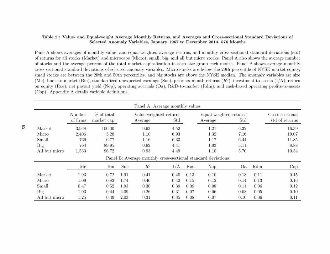
Table 2 : Value- and Equal-weight Average Monthly Returns, and Averages and Cross-sectional Standard Deviations ofSelected Anomaly Variables, January 1967 to December 2014, 576 Months

Pane A shows averages of monthly value- and equal-weighted average returns, and monthly cross-sectional standard deviations (std)of returns for all stocks (Market) and microcaps (Micro), small, big, and all but micro stocks. Panel A also shows the average numberof stocks and the average percent of the total market capitalization in each size group each month. Panel B shows average monthlycross-sectional standard deviations of selected anomaly variables. Micro stocks are below the 20th percentile of NYSE market equity,small stocks are between the 20th and 50th percentiles, and big stocks are above the NYSE median. The anomaly variables are size(Me), book-to-market (Bm), standardized unexpected earnings (Sue), prior six-month returns (R6), investment-to-assets (I/A), returnon equity (Roe), net payout yield (Nop), operating accruals (Oa), R&D-to-market (Rdm), and cash-based operating profits-to-assets(Cop). Appendix A details variable definitions.

Panel A: Average monthly values

Number % of total Value-weighted returns Equal-weighted returns Cross-sectionalof firms market cap Average Std Average Std std of returns

Market 3,938 100.00 0.93 4.52 1.21 6.32 16.39Micro 2,406 3.28 1.10 6.93 1.32 7.16 19.07Small 769 6.77 1.16 6.33 1.17 6.44 11.85Big 764 89.95 0.92 4.41 1.03 5.11 8.88All but micro 1,533 96.72 0.93 4.49 1.10 5.70 10.54

Panel B: Average monthly cross-sectional standard deviations

Me Bm Sue R6 I/A Roe Nop Oa Rdm Cop

Market 1.93 0.72 1.91 0.41 0.40 0.13 0.10 0.13 0.11 0.15Micro 1.09 0.82 1.74 0.46 0.42 0.15 0.12 0.14 0.13 0.16Small 0.47 0.52 1.93 0.36 0.39 0.09 0.08 0.11 0.06 0.12Big 1.03 0.44 2.09 0.26 0.31 0.07 0.06 0.08 0.05 0.10All but micro 1.25 0.49 2.03 0.31 0.35 0.08 0.07 0.10 0.06 0.11

62

Table 3 : Anomalies That Cannot Be Replicated at the 5% Significance Level, January 1967to December 2014, 576 Months

Insignificant anomalies are defined as those with the average returns of their high-minus-lowdeciles insignificant at the 5% level. For each insignificant anomaly, this table reports the averagereturn (m) and its t-statistics for the high-minus-low decile. The t-statistics are adjusted forheteroscedasticity and autocorrelations. The number in parentheses in the title of each paneldenotes the number insignificant anomalies in the category of anomalies in question. Table 1describes the symbols. Appendix A details variable definitions and portfolio construction.

Panel A: Momentum (20)

Sue6 Sue12 Re12 R1112 Rs6 Rs12 Tes1 Tes6 Tes12 Nei12 52w1 52w12 ǫ61 Sm6

m 0.19 0.11 0.28 0.43 0.14 0.06 0.26 0.28 0.18 0.14 0.14 0.45 0.20 0.09tm 1.65 1.00 1.47 1.92 1.01 0.44 1.56 1.90 1.34 1.36 0.43 1.88 1.20 0.88

Sm12 Ile6 Ile12 Cm6 Sim6 Sim12

m 0.14 0.27 0.11 0.18 0.12 0.15tm 1.87 1.79 0.84 1.83 1.11 1.80

Panel B: Value-versus-growth (37)

Bmq1 Bmq6 Dm Dmq1 Dmq6 Dmq12 Am Amq1 Amq6 Amq12 Efp6 Efp12 Dp Dpq1

m 0.46 0.45 0.31 0.30 0.27 0.32 0.36 0.37 0.42 0.40 0.43 0.40 0.21 0.26tm 1.79 1.90 1.59 1.26 1.17 1.50 1.72 1.33 1.58 1.69 1.78 1.71 0.86 1.02

Dpq6 Dpq12 Op Opq1 Opq6 Opq12 Nopq1 Nopq6 Nopq12 Sr Sg Ocpq6 Ocpq12 Ebpq1

m 0.19 0.20 0.37 0.10 0.10 0.17 0.22 0.25 0.31 −0.20 −0.01 0.51 0.41 0.27tm 0.76 0.85 1.70 0.42 0.52 0.87 0.91 1.14 1.48 −1.08 −0.08 1.89 1.71 1.00

Ebpq6 Ebpq12 Ndp Ndpq1 Ndpq6 Ndpq12 Ltg1 Ltg6 Ltg12

m 0.26 0.35 0.31 0.17 0.18 0.27 −0.03 −0.04 −0.01tm 1.01 1.44 1.62 0.71 0.77 1.22 −0.09 −0.10 −0.02

Panel C: Investment (11)

Iaq1 3Ig Cdi Ta dCol dNcl dSti dLti dBe Nxf Nef

m −0.32 −0.21 −0.00 −0.23 −0.11 −0.11 0.15 −0.22 −0.31 −0.27 −0.17tm −1.72 −1.46 −0.01 −1.63 −0.76 −0.95 0.98 −1.44 −1.89 −1.44 −0.86

Panel D: Profitability (46)

Roe6 Roe12 Roa6 Roa12 dRoa12 Rna Pm Ato Cto Rnaq1 Rnaq12 Pmq1 Pmq6 Pmq12

m 0.42 0.24 0.39 0.25 0.21 0.12 0.01 0.32 0.27 0.43 0.35 0.35 0.17 0.18tm 1.95 1.19 1.78 1.26 1.78 0.63 0.03 1.76 1.60 1.95 1.63 1.59 0.82 0.89

Gla Ope Ole Oleq12 Opa Ola F Fp Fpq1 Fpq12 O Oq1 Oq6 Oq12

m 0.16 0.25 0.07 0.35 0.37 0.20 0.29 −0.38 −0.48 −0.36 −0.06 −0.36 −0.21 −0.14tm 1.04 1.20 0.37 1.78 1.87 1.07 1.06 −1.28 −1.43 −1.25 −0.30 −1.57 −0.96 −0.64

Z Zq1 Zq6 Zq12 G Cr1 Cr6 Cr12 Tbi Tbiq1 Tbiq6 Bl Blq1 Blq6

m −0.00 0.01 −0.03 −0.09 0.27 0.04 0.01 0.01 0.16 0.17 0.21 −0.02 0.10 0.13tm −0.02 0.06 −0.15 −0.46 1.35 0.12 0.02 0.03 1.20 1.28 1.84 −0.10 0.58 0.73

Blq12 Sgq1 Sgq6 Sgq12

m 0.10 0.32 0.14 −0.06tm 0.55 1.81 0.86 −0.40

63

Panel E: Intangibles (77)

gAd Rds Rdsq1 Rdsq6 Rdsq12 Hn Rca Bca Aop Pafe Parc Crd Ha He

m −0.06 0.08 0.33 0.44 0.47 −0.27 0.34 0.17 −0.21 0.20 0.09 0.16 −0.23 −0.22tm −0.31 0.31 1.08 1.57 1.68 −1.79 1.40 0.71 −1.18 0.58 0.39 0.64 −1.54 −1.48

Age1 Age6 Age12 D1 D2 D3 dSi dSa dGs dSs Lfe Ana1 Ana6 Ana12

m 0.01 0.02 0.00 0.21 0.27 0.27 0.14 0.16 0.06 0.04 0.20 −0.15 −0.12 −0.11tm 0.04 0.09 0.02 0.97 1.22 1.25 1.02 1.25 0.46 0.24 1.59 −0.89 −0.73 −0.65

Tan Tanq1 Tanq6 Tanq12 Kz Kzq1 Kzq6 Kzq12 Ww Wwq1 Wwq6 Wwq12 Sdd Cdd

m 0.04 0.22 0.21 0.15 −0.09 −0.11 −0.13 −0.11 0.22 0.04 0.09 0.09 0.09 −0.05tm 0.27 1.14 1.22 0.93 −0.46 −0.56 −0.64 −0.56 0.90 0.16 0.31 0.32 0.36 −0.21

Vcf1 Vcf6 Vcf12 Cta1 Cta6 Cta12 Gind Acq Acq1 Acq6 Acq12 Ob Eper Esm

m −0.37 −0.33 −0.27 0.22 0.11 0.09 0.02 −0.07 −0.06 −0.03 −0.01 0.17 0.01 −0.06tm −1.68 −1.56 −1.31 1.08 0.55 0.45 0.06 −0.36 −0.28 −0.13 −0.06 0.71 0.10 −0.45

Evr Ecs Frm Fra Ala Alm Alaq1 Alaq6 Alaq12 Dls1 Dls6 Dls12 Dis1 Dis6

m 0.18 0.07 0.09 −0.11 −0.10 0.14 0.42 0.28 0.19 −0.24 0.01 0.06 −0.24 −0.22tm 1.32 0.65 0.46 −0.77 −0.49 0.73 1.68 1.12 0.79 −1.19 0.05 0.44 −0.89 −0.87

Dis12 Dlg1 Dlg6 Dlg12 R1n R

[11,15]n R

[16,20]n

m −0.13 −0.13 −0.08 −0.10 0.54 −0.31 −0.26tm −0.53 −0.52 −0.34 −0.41 1.74 −1.86 −1.60

Panel F: Trading frictions (95)

Me Iv Ivff1 Ivff6 Ivff12 Ivc1 Ivc6 Ivc12 Ivq1 Ivq6 Ivq12 Tv1 Tv6 Tv12

m −0.28 −0.22 −0.51 −0.33 −0.18 −0.48 −0.32 −0.20 −0.48 −0.30 −0.19 −0.40 −0.25 −0.20tm −1.12 −0.66 −1.62 −1.11 −0.62 −1.48 −1.07 −0.69 −1.53 −1.05 −0.68 −1.16 −0.77 −0.62

Sv6 Sv12 β1 β6 β12 βFP1 βFP6 βFP12 βD1 βD6 βD12 Tur1 Tur6 Tur12

m −0.19 −0.16 0.06 0.06 0.01 −0.22 −0.23 −0.18 0.04 0.05 0.03 −0.15 −0.14 −0.10tm −1.36 −1.43 0.18 0.17 0.04 −0.65 −0.72 −0.57 0.21 0.30 0.19 −0.57 −0.53 −0.38

Cvt1 Cvt6 Cvt12 Dtv1 Cvd1 Cvd6 Cvd12 Pps1 Pps6 Pps12 Ami1 Ami6 Lm11 Lm16

m 0.13 0.11 0.17 −0.27 0.10 0.12 0.18 −0.02 0.04 −0.04 0.28 0.37 −0.07 0.21tm 0.87 0.73 1.26 −1.45 0.65 0.85 1.25 −0.06 0.15 −0.14 1.31 1.73 −0.33 0.95

Lm112 Lm61 Lm66 Lm612 Lm121 Lm126 Lm1212 Mdr1 Mdr6 Mdr12 Ts6 Ts12 Isc1 Isc6

m 0.20 0.38 0.35 0.30 0.38 0.33 0.24 −0.34 −0.17 −0.07 0.03 0.03 0.17 −0.02tm 0.93 1.82 1.67 1.40 1.78 1.57 1.13 −1.14 −0.62 −0.24 0.50 0.56 1.66 −0.33

Isc12 Isff6 Isff12 Isq1 Isq12 Cs1 Cs6 Cs12 Srev β−1 β−6 β−12 Tail1 Tail6

m 0.05 0.08 0.10 0.07 0.08 −0.10 −0.02 −0.03 −0.26 −0.12 −0.17 −0.12 0.11 0.15tm 1.04 1.48 1.88 1.14 1.71 −0.85 −0.40 −0.59 −1.31 −0.41 −0.60 −0.45 0.57 0.79

Tail12 βret1 βret6 βret12 βlcc1 βlcc6 βlcc12 βlrc1 βlrc6 βlrc12 βlcr1 βlcr6 βlcr12 βnet1

m 0.19 0.05 0.04 0.01 0.34 0.31 0.31 0.05 0.02 0.05 0.06 −0.02 −0.05 0.14tm 1.13 0.16 0.12 0.03 1.54 1.45 1.49 0.17 0.07 0.17 0.46 −0.17 −0.49 0.41

βnet6 βnet12 Shl1 Shl6 Shl12 Sba1 Sba6 Sba12 βLev1 βLev6 βLev12

m 0.15 0.10 −0.16 −0.16 −0.12 −0.20 −0.10 −0.07 0.43 0.30 0.25tm 0.47 0.32 −0.54 −0.57 −0.45 −0.73 −0.36 −0.26 1.78 1.31 1.15

64

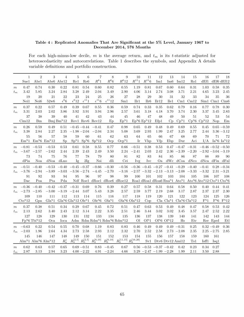
Table 4 : Replicated Anomalies That Are Significant at the 5% Level, January 1967 toDecember 2014, 576 Months

For each high-minus-low decile, m is the average return, and tm is its t-statistic adjusted forheteroscedasticity and autocorrelations. Table 1 describes the symbols, and Appendix A detailsvariable definitions and portfolio construction.

1 2 3 4 5 6 7 8 9 10 11 12 13 14 15 16 17 18Sue1 Abr1 Abr6 Abr12 Re1 Re6 R61 R66 R612 R111 R116 Im1 Im6 Im12 Rs1 dEf1 dEf6 dEf12

m 0.47 0.74 0.30 0.22 0.81 0.54 0.60 0.82 0.55 1.19 0.81 0.67 0.60 0.64 0.31 1.03 0.58 0.35tm 3.42 5.85 3.24 2.84 3.28 2.49 2.04 3.49 2.90 4.06 3.14 2.74 3.08 3.71 2.21 4.65 3.23 2.45

19 20 21 22 23 24 25 26 27 28 29 30 31 32 33 34 35 36Nei1 Nei6 52w6 ǫ66 ǫ612 ǫ111 ǫ116 ǫ1112 Sm1 Ilr1 Ilr6 Ilr12 Ile1 Cm1 Cm12 Sim1 Cim1 Cim6

m 0.37 0.22 0.57 0.49 0.39 0.67 0.55 0.36 0.59 0.74 0.33 0.35 0.62 0.79 0.16 0.77 0.78 0.30tm 3.31 2.03 2.02 3.86 3.92 3.91 3.94 2.96 2.57 3.61 3.18 4.18 3.70 3.74 2.30 3.37 3.45 2.83

37 38 39 40 41 42 43 44 45 46 47 48 49 50 51 52 53 54Cim12 Bm Bmj Bmq12 Rev1 Rev6 Rev12 Ep Epq1 Epq6 Epq12 Efp1 Cp Cpq1 Cpq6 Cpq12 Nop Em

m 0.26 0.59 0.49 0.51 −0.45 −0.44 −0.41 0.47 0.98 0.65 0.49 0.48 0.49 0.69 0.55 0.45 0.65 −0.59tm 3.38 2.84 2.27 2.35 −1.98 −2.04 −2.04 2.34 5.08 3.69 2.93 1.99 2.47 3.25 2.77 2.44 3.36 −3.12

55 56 57 58 59 60 61 62 63 64 65 66 67 68 69 70 71 72Emq1 Emq6 Emq12 Sp Spq1 Spq6 Spq12 Ocp Ocpq1 Ir Vhp Vfp Ebp Dur Aci I/A Iaq6 Iaq12

m −0.81 −0.53 −0.53 0.53 0.61 0.58 0.55 0.77 0.66 −0.51 0.38 0.53 0.47 −0.47 −0.31 −0.46 −0.52 −0.50tm −3.67 −2.57 −2.62 2.44 2.39 2.43 2.49 3.50 2.24 −2.41 2.03 2.42 2.36 −2.39 −2.20 −2.92 −3.04 −3.19

73 74 75 76 77 78 79 80 81 82 83 84 85 86 87 88 89 90dPia Noa dNoa dLno Ig 2Ig Nsi dIi Cei Ivg Ivc Oa dWc dCoa dNco dNca dFin dFnl

m −0.51 −0.40 −0.53 −0.40 −0.45 −0.37 −0.66 −0.30 −0.56 −0.36 −0.45 −0.27 −0.41 −0.29 −0.40 −0.41 0.28 −0.34tm −3.76 −2.94 −3.89 −3.03 −3.56 −2.74 −4.45 −2.70 −3.16 −2.57 −3.32 −2.13 −3.13 −2.08 −3.33 −3.32 2.31 −3.21

91 92 93 94 95 96 97 98 99 100 101 102 103 104 105 106 107 108Dac Poa Pta Pda Ndf Roe1 dRoe1 dRoe6 dRoe12 Roa1 dRoa1 dRoa6 Rnaq1 Atoq1 Atoq6 Atoq12 Ctoq1 Ctoq6

m −0.36 −0.40 −0.42 −0.37 −0.31 0.69 0.76 0.39 0.27 0.57 0.58 0.31 0.64 0.58 0.50 0.40 0.44 0.41tm −2.73 −2.85 −3.00 −3.19 −2.44 3.07 5.43 3.28 2.57 2.59 3.77 2.19 2.68 3.17 2.87 2.37 2.37 2.30

109 110 111 112 113 114 115 116 117 118 119 120 121 122 123 124 125 126Ctoq12 Gpa Glaq1 Glaq6 Glaq12 Oleq1 Oleq6 Olaq1 Olaq6 Olaq12 Cop Cla Claq1 Claq6 Claq12 Fq1 Fq6 Fq12

m 0.37 0.38 0.51 0.34 0.29 0.67 0.45 0.72 0.51 0.47 0.63 0.53 0.49 0.48 0.47 0.58 0.53 0.42tm 2.13 2.62 3.40 2.43 2.12 3.14 2.22 3.35 2.51 2.46 3.44 3.02 3.02 3.45 3.57 2.47 2.52 2.22

127 128 129 130 131 132 133 134 135 136 137 138 139 140 141 142 143 144Fpq6 Tbiq12 Oca Ioca Adm Rdm Rdmq1 Rdmq6 Rdmq12 Ol Olq1 Olq6 Olq12 Hs Etr Rer Eprd Etl

m −0.63 0.22 0.54 0.55 0.70 0.68 1.19 0.83 0.83 0.46 0.49 0.49 0.49 −0.31 0.25 0.32 −0.49 0.36tm −2.03 1.96 2.64 4.34 2.73 2.58 2.93 2.12 2.32 2.70 2.52 2.58 2.73 −2.08 2.35 2.25 −2.75 2.85

145 146 147 148 149 150 151 152 153 154 155 156 157 158 159 160 161

Almq1 Almq6 Almq12 R1a R

[2,5]a R

[2,5]n R

[6,10]a R

[6,10]n R

[11,15]a R

[16,20]a Sv1 Dtv6 Dtv12 Ami12 Ts1 Isff1 Isq1

m 0.62 0.63 0.57 0.65 0.69 −0.51 0.83 −0.45 0.67 0.56 −0.53 −0.37 −0.42 0.42 0.23 0.34 0.27tm 2.87 3.13 2.94 3.23 4.00 −2.22 4.91 −2.24 4.66 3.29 −2.47 −1.99 −2.28 1.99 2.11 3.50 2.88

65

Table 5 : Average Return Spreads and Their t-values for High-minus-low Anomaly Decileswith NYSE Breakpoints and Value-weighted Returns in the Original Samples

Insignificant anomalies are identified as those with the average returns of the high-minus-low decilesinsignificant at the 5% level, and significant anomalies are those with significant average returnspreads. For the high-minus-low decile formed on each anomaly variable, this table reports theaverage return (m) and its t-statistic adjusted for heteroscedasticity and autocorrelations. Table 1describes the symbols, and Appendix A details variable definitions and portfolio construction.

Panel A: Momentum

Insignificant (24)

Sue1 Sue6 Sue12 Re6 Re12 Rs1 Rs6 Rs12 Tes1 Tes12 dEf12 Nei1 Nei6 Nei12

m 0.50 0.37 0.00 0.59 0.27 0.31 0.24 0.24 0.26 0.28 0.84 0.44 0.29 0.23tm 1.14 0.85 0.01 1.78 0.86 1.15 0.93 0.99 1.40 1.82 1.80 1.82 1.20 0.98

52w1 ǫ61 Sm6 Sm12 Ile6 Ile12 Cm6 Cm12 Sim6 Sim12

m 0.35 0.29 0.14 0.16 0.27 0.11 0.15 0.14 0.15 0.18tm 1.09 1.58 1.29 1.85 1.60 0.74 1.19 1.62 1.20 1.76

Significant (33)

Abr1 Abr6 Abr12 Re1 R61 R66 R612 R111 R116 R1112 Im1 Im6 Im12 Tes6

m 0.96 0.41 0.30 1.07 0.90 1.06 0.85 1.58 1.26 0.79 0.76 0.69 0.75 0.37tm 5.35 3.41 2.70 3.10 2.95 3.82 3.66 4.95 4.48 3.17 2.68 2.90 3.71 2.19

dEf1 dEf6 52w6 52w12 ǫ66 ǫ612 ǫ111 ǫ116 ǫ1112 Sm1 Ilr1 Ilr6 Ilr12 Ile1

m 1.91 1.47 0.86 0.65 0.56 0.45 0.77 0.62 0.38 0.64 0.83 0.36 0.41 0.63tm 3.68 2.89 3.15 2.66 4.12 4.12 4.11 4.07 2.88 2.54 3.57 2.94 4.27 3.36

Cm1 Sim1 Cim1 Cim6 Cim12

m 0.89 0.88 0.90 0.34 0.29tm 3.34 3.23 3.44 2.79 3.22

Panel B: Value-versus-growth

Insignificant (44)

Bmq1 Dm Dmq1 Dmq6 Dmq12 Am Amq1 Amq6 Amq12 Epq12 Efp1 Efp6 Efp12 Dp

m 0.54 0.51 0.94 0.92 0.87 0.38 0.27 0.27 0.30 0.64 −0.01 −0.07 −0.03 0.49tm 1.959 1.38 1.55 1.69 1.70 1.44 0.91 0.95 1.10 1.84 −0.03 −0.26 −0.12 1.10

Dpq1 Dpq6 Dpq12 Opq1 Opq6 Opq12 Nopq1 Nopq6 Nopq12 Sg Sp Spq1 Spq6 Spq12

m 0.50 0.46 0.44 0.24 0.17 0.28 0.41 0.47 0.53 −0.20 0.41 0.24 0.20 0.29tm 1.10 1.04 0.99 0.77 0.61 1.06 1.20 1.47 1.72 −0.91 1.30 0.69 0.60 0.95

Ocpq1 Ocpq6 Ocpq12 Vhp Vfp Ebp Ebpq1 Ebpq6 Ebpq12 Ndp Ndpq1 Ndpq6 Ndpq12 Ltg1

m 0.16 0.12 0.10 0.19 0.33 0.43 0.22 0.19 0.33 0.23 −0.10 −0.04 0.11 0.05tm 0.50 0.41 0.38 0.63 1.15 1.88 0.70 0.63 1.19 1.08 −0.34 −0.16 0.43 0.07

Ltg6 Ltg12

m −0.05 0.01tm −0.07 0.02

Significant (24)

Bm Bmj Bmq6 Bmq12 Rev1 Rev6 Rev12 Ep Epq1 Epq6 Cp Cpq1 Cpq6 Cpq12

m 1.41 0.53 0.50 0.55 −0.87 −0.81 −0.76 0.77 1.17 0.81 0.77 0.84 0.63 0.63tm 3.09 2.31 2.00 2.43 −2.11 −2.06 −2.06 1.97 2.91 2.26 2.65 2.88 2.35 2.45

Op Nop Sr Em Emq1 Emq6 Emq12 Ocp Ir Dur

m 0.56 0.89 −0.45 −0.67 −0.91 −0.61 −0.61 0.54 −0.63 −0.63tm 2.11 3.71 −1.99 −3.25 −3.69 −2.64 −2.72 2.03 −2.40 −2.64

66

Panel C: Investment

Insignificant (13)

Iaq1 3Ig dIi Cdi Ta dCol dNcl dLti dBe Poa Pta Pda Nef

m −0.44 −0.15 −0.28 0.01 −0.30 −0.11 −0.22 −0.29 −0.38 −0.41 −0.23 −0.34 −0.32tm −1.89 −0.80 −1.82 0.06 −1.82 −0.65 −1.57 −1.61 −1.86 −1.70 −0.92 −1.87 −1.35

Significant (25)

Aci Ia Iaq6 Iaq12 dPia Noa dNoa dLno Ig 2Ig Nsi Cei Ivg Ivc

m −0.39 −0.58 −0.69 −0.66 −0.55 −0.46 −0.47 −0.39 −0.55 −0.34 −0.87 −0.69 −0.45 −0.45tm −2.51 −3.05 −3.26 −3.40 −3.61 −2.75 −3.18 −2.32 −3.91 −2.13 −4.80 −3.13 −3.17 −2.62

Oa dWc dCoa dNco dNca dFin dSti dFnl Dac Nxf Ndf

m −0.33 −0.53 −0.40 −0.48 −0.51 0.36 0.40 −0.38 −0.38 −0.44 −0.36tm −1.97 −3.35 −2.47 −3.40 −3.46 2.50 2.23 −2.99 −2.42 −1.97 −2.23

Panel D: Profitability

Insignificant (38)

Roe6 Roe12 Roa6 Roa12 Rna Pm Ato Cto Rnaq12 Pmq1 Pmq6 Pmq12 Ctoq6 Ctoq12

m 0.48 0.28 0.35 0.27 0.34 0.37 0.48 0.44 0.63 0.69 0.49 0.45 0.61 0.56tm 1.93 1.23 1.34 1.11 1.09 0.91 1.47 1.26 1.90 1.61 1.21 1.15 1.80 1.63

Gla Ope Ole Oleq12 Opa Ola Z Zq1 Zq6 Zq12 Cr1 Cr6 Cr12 Tbi

m 0.17 0.26 0.07 0.36 0.34 0.17 −0.04 0.08 0.06 −0.01 −0.07 −0.11 −0.08 0.14tm 1.07 1.21 0.36 1.81 1.69 0.91 −0.13 0.23 0.18 −0.02 −0.19 −0.28 −0.21 0.66

Tbiq1 Tbiq6 Tbiq12 Bl Blq1 Blq6 Blq12 Sgq1 Sgq6 Sgq12

m 0.18 0.24 0.27 −0.02 0.14 0.19 0.13 0.30 0.06 −0.23tm 0.82 1.17 1.34 −0.10 0.68 0.93 0.63 1.19 0.27 −1.08

Significant (41)

Roe1 dRoe1 dRoe6 dRoe12 Roa1 dRoa1 dRoa6 dRoa12 Rnaq1 Rnaq6 Atoq1 Atoq6 Atoq12 Ctoq1

m 0.82 0.83 0.42 0.31 0.68 0.71 0.39 0.31 0.89 0.69 0.94 0.80 0.64 0.69tm 3.22 5.36 3.17 2.66 2.50 4.24 2.52 2.25 2.39 2.00 3.27 2.91 2.32 2.06

Gpa Glaq1 Glaq6 Glaq12 Oleq1 Oleq6 Olaq1 Olaq6 Olaq12 Cop Cla Claq1 Claq6 Claq12

m 0.41 0.53 0.38 0.32 0.68 0.47 0.71 0.49 0.45 0.63 0.53 0.49 0.48 0.47tm 2.64 3.28 2.53 2.26 3.12 2.25 3.21 2.34 2.29 3.44 3.02 3.02 3.45 3.57

F Fq1 Fq6 Fq12 Fp Fpq1 Fpq6 Fpq12 O Oq1 Oq6 Oq12 G

m 0.65 0.65 0.61 0.55 −0.82 −0.96 −1.15 −0.74 −0.60 −0.84 −0.76 −0.69 0.70tm 2.19 2.36 2.43 2.55 −2.10 −2.31 −2.92 −2.04 −2.06 −2.73 −2.50 −2.29 2.69

Panel E: Intangibles

Insignificant (81)

gAd Rdm Rdmq1 Rdmq6 Rdmq12 Rds Rdsq1 Rdsq6 Rdsq12 Hn Rca Bca Aop Pafe

m −0.13 0.47 1.12 0.79 0.76 0.08 0.46 0.69 0.73 −0.30 0.31 0.28 −0.16 −0.06tm −0.63 1.38 1.76 1.21 1.43 0.25 0.98 1.66 1.87 −1.82 1.08 1.01 −0.60 −0.09

Parc Crd Ha He Age1 Age6 Age12 D1 D2 D3 dSi dGs dSs Etr

m 0.09 0.16 −0.27 −0.28 0.07 0.07 0.05 0.17 0.23 0.24 0.05 0.10 −0.10 0.20tm 0.39 0.64 −1.56 −1.62 0.28 0.29 0.24 0.67 0.87 0.90 0.27 0.54 −0.54 1.46

Lfe Ana1 Ana6 Ana12 Tan Tanq1 Tanq6 Tanq12 Kz Kzq1 Kzq6 Kzq12 Ww Wwq1

m 0.12 0.33 0.38 0.39 −0.11 0.06 −0.01 −0.08 −0.19 −0.24 −0.26 −0.27 0.25 0.08tm 0.69 1.32 1.53 1.59 −0.64 0.26 −0.05 −0.44 −0.85 −0.93 −1.01 −1.02 0.67 0.20

Wwq6 Wwq12 Sdd Cdd Vcf12 Cta1 Cta6 Cta12 Acq Acq1 Acq6 Acq12 Ob Eper

m 0.13 0.14 0.16 −0.06 −0.50 0.19 0.05 0.04 −0.17 −0.19 −0.17 −0.15 0.09 −0.04tm 0.34 0.35 0.56 −0.16 −1.79 0.83 0.24 0.16 −0.60 −0.69 −0.59 −0.54 0.24 −0.23

67

Esm Evr Etl Ecs Frm Fra Ala Alm Alaq1 Alaq6 Alaq12 Almq1 Almq12 Dls1

m −0.06 0.18 0.31 0.09 0.31 −0.13 −0.10 −0.05 0.36 0.16 0.14 0.56 0.47 −0.19tm −0.31 0.86 1.72 0.63 1.21 −0.65 −0.35 −0.20 0.98 0.43 0.40 1.89 1.77 −0.83

Dls6 Dls12 Dis1 Dis6 Dis12 Dlg1 Dlg6 Dlg12 R[6,10]n R

[11,15]n R

[16,20]n

m 0.05 0.08 −0.62 −0.60 −0.47 −0.25 −0.26 −0.21 −0.41 −0.29 −0.27tm 0.27 0.44 −1.47 −1.47 −1.22 −0.66 −0.67 −0.57 −1.64 −1.45 −1.42

Significant (22)

Oca Ioca Adm Ol Olq1 Olq6 Olq12 Hs dSa Rer Vcf1 Vcf6 Gind Eprd

m 0.51 0.59 0.83 0.50 0.53 0.54 0.55 −0.38 0.29 0.40 −0.60 −0.57 −0.73 −0.54tm 2.16 4.21 2.74 2.66 2.44 2.55 2.76 −2.34 2.02 2.43 −2.02 −2.03 −2.04 −2.33

Almq6 R1a R1

n R[2,5]a R

[2,5]n R

[6,10]a R

[11,15]a R

[16,20]a

m 0.59 0.93 0.77 0.97 −0.81 0.94 0.84 0.67tm 2.17 3.89 2.26 4.97 −2.92 4.75 4.96 3.34

Panel F: Trading frictions

Insignificant (93)

Me Iv Ivff6 Ivff12 Ivc1 Ivc6 Ivc12 Ivq6 Ivq12 Tv1 Tv6 Tv12 Sv6 Sv12

m −0.26 −0.14 −0.42 −0.25 −0.69 −0.42 −0.27 −0.42 −0.28 −0.55 −0.33 −0.24 −0.27 −0.27tm −0.41 −0.31 −1.26 −0.74 −1.89 −1.24 −0.82 −1.27 −0.87 −1.43 −0.88 −0.66 −1.37 −1.70

β1 β6 β12 βFP1 βFP6 βFP12 βD1 βD6 βD12 Tur1 Tur6 Tur12 Cvt1 Cvt6

m 2.33 1.95 1.82 −0.17 −0.19 −0.14 −0.04 −0.14 −0.19 −0.31 −0.27 −0.24 0.14 0.16tm 1.85 1.57 1.43 −0.48 −0.58 −0.43 −0.11 −0.50 −0.73 −0.99 −0.85 −0.76 0.88 1.06

Cvt12 Dtv1 Dtv6 Dtv12 Cvd1 Cvd6 Cvd12 Pps1 Pps6 Pps12 Ami1 Ami6 Ami12 Lm11

m 0.26 −0.20 −0.29 −0.36 0.15 0.17 0.27 −0.69 −0.44 −0.48 0.18 0.27 0.34 −0.07tm 1.72 −0.88 −1.30 −1.66 0.93 1.08 1.79 −1.12 −0.75 −0.84 0.68 1.06 1.33 −0.27

Lm16 Lm112 Lm612 Lm126 Lm1212 Mdr1 Mdr6 Mdr12 Ts1 Ts6 Ts12 Isc1 Isc6 Isc12

m 0.32 0.31 0.43 0.45 0.39 −0.39 −0.22 −0.10 0.22 0.02 0.02 0.17 −0.03 0.05tm 1.28 1.29 1.84 1.89 1.60 −1.19 −0.69 −0.33 1.93 0.27 0.42 1.57 −0.45 0.91

Isff6 Isff12 Isq6 Isq12 Cs1 Cs6 Cs12 β−1 β−6 β−12 Tail1 Tail6 Tail12 βret1

m 0.08 0.09 0.06 0.08 0.07 −0.05 −0.08 −0.18 −0.20 −0.12 0.11 0.14 0.19 0.19tm 1.33 1.70 1.00 1.65 0.54 −0.79 −1.49 −0.58 −0.65 −0.42 0.52 0.69 1.04 0.51

βret6 βret12 βlcc1 βlcc6 βlcc12 βlrc1 βlrc6 βlrc12 βlcr1 βlcr6 βlcr12 βnet1 βnet6 βnet12

m 0.22 0.20 0.25 0.27 0.29 0.07 0.10 0.07 0.06 0.03 −0.02 0.34 0.39 0.34tm 0.59 0.55 0.94 1.03 1.15 0.23 0.31 0.24 0.37 0.23 −0.12 0.93 1.06 0.95

Shl1 Shl6 Shl12 Sba1 Sba6 Sba12 βlev1 βlev6 βlev12

m −0.16 −0.21 −0.15 −0.21 −0.12 −0.12 0.46 0.30 0.25tm −0.51 −0.71 −0.56 −0.75 −0.46 −0.44 1.72 1.19 1.00

Significant (9)

Ivff1 Ivq1 Sv1 Lm61 Lm66 Lm121 Isf1 Isq1 Srev

m −0.72 −0.71 −0.99 0.49 0.49 0.49 0.34 0.27 −0.65tm −2.01 −1.97 −3.30 2.09 2.08 2.03 3.38 2.86 −2.40

68

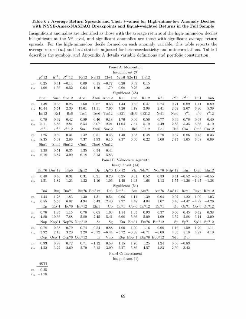
Table 6 : Average Return Spreads and Their t-values for High-minus-low Anomaly Decileswith NYSE-Amex-NASDAQ Breakpoints and Equal-weighted Returns in the Full Sample

Insignificant anomalies are identified as those with the average returns of the high-minus-low decilesinsignificant at the 5% level, and significant anomalies are those with significant average returnspreads. For the high-minus-low decile formed on each anomaly variable, this table reports theaverage return (m) and its t-statistic adjusted for heteroscedasticity and autocorrelations. Table 1describes the symbols, and Appendix A details variable definitions and portfolio construction.

Panel A: Momentum

Insignificant (9)

R612 R116 R1112 Rs12 Nei12 52w1 52w6 52w12 Ile12

m 0.25 0.41 −0.14 0.09 0.15 −0.77 0.26 0.09 0.15tm 1.08 1.36 −0.52 0.64 1.10 −1.79 0.68 0.26 1.20

Significant (48)

Sue1 Sue6 Sue12 Abr1 Abr6 Abr12 Re1 Re6 Re12 R61 R66 R111 Im1 Im6

m 1.38 0.68 0.26 1.60 0.87 0.53 1.43 0.85 0.47 0.74 0.71 0.89 1.41 0.89tm 10.44 5.51 2.30 15.61 11.11 7.96 7.26 4.78 2.98 2.41 2.62 2.67 6.90 5.39

Im12 Rs1 Rs6 Tes1 Tes6 Tes12 dEf1 dEf6 dEf12 Nei1 Nei6 ǫ61 ǫ66 ǫ612

m 0.78 0.92 0.42 0.89 0.46 0.18 1.76 0.96 0.56 0.77 0.39 0.76 0.67 0.40tm 5.11 5.86 2.81 8.54 5.07 2.21 11.04 7.57 5.19 5.49 2.83 5.35 5.66 4.10

ǫ111 ǫ116 ǫ1112 Sm1 Sm6 Sm12 Ilr1 Ilr6 Ilr12 Ile1 Ile6 Cm1 Cm6 Cm12

m 1.25 0.69 0.31 1.42 0.51 0.45 1.40 0.63 0.48 0.78 0.37 0.86 0.43 0.33tm 8.35 5.37 2.86 7.37 4.93 6.16 8.37 6.60 6.22 5.00 2.74 5.65 6.38 6.09

Sim1 Sim6 Sim12 Cim1 Cim6 Cim12

m 1.38 0.51 0.35 1.35 0.54 0.44tm 6.18 3.87 3.90 6.18 5.13 5.83

Panel B: Value-versus-growth

Insignificant (14)

Dmq6 Dmq12 Efp6 Efp12 Dp Dpq6 Dpq12 Vfp Ndpq1 Ndpq6 Ndpq12 Ltg1 Ltg6 Ltg12

m 0.40 0.46 0.31 0.31 0.21 0.20 0.25 0.31 0.52 0.33 0.41 −0.52 −0.58 −0.55tm 1.51 1.82 1.23 1.32 1.10 1.06 1.40 1.43 1.68 1.13 1.57 −1.26 −1.47 −1.38

Significant (54)

Bm Bmj Bmq1 Bmq6 Bmq12 Dm Dmq1 Am Amq1 Amq6 Amq12 Rev1 Rev6 Rev12

m 1.44 1.28 1.83 1.30 1.31 0.54 0.66 1.11 1.39 0.94 0.97 −1.22 −1.09 −1.03tm 6.55 5.53 6.07 4.94 5.43 2.40 2.27 4.48 4.04 3.07 3.46 −4.47 −4.22 −4.26

Ep Epq1 Eoq6 Epq12 Efp1 Cp Cpq1 Cpq6 Cpq12 Dpq1 Op Opq1 Opq6 Opq12

m 0.76 1.85 1.15 0.76 0.65 1.03 1.54 1.05 0.93 0.37 0.60 0.45 0.42 0.38tm 4.80 10.36 7.88 5.89 2.45 5.41 6.98 5.36 5.09 1.99 3.52 2.88 3.11 3.00

Nop Nopq1 Nopq6 Nopq12 Sr Sg Em Emq1 Emq6 Emq12 Sp Spq1 Spq6 Spq12

m 0.78 0.58 0.79 0.74 −0.54 −0.88 −1.00 −1.90 −1.16 −0.98 1.16 1.59 1.20 1.11tm 3.92 2.18 3.20 3.20 −3.72 −6.44 −5.72 −8.88 −6.71 −6.08 4.35 5.18 4.27 4.10

Ocp Ocpq1 Ocpq6 Ocpq12 Ir Vhp Ebp Ebpq1 Ebpq6 Ebpq12 Ndp Dur

m 0.93 0.99 0.72 0.71 −1.12 0.59 1.15 1.76 1.25 1.24 0.50 −0.83tm 4.52 3.22 2.60 2.79 −5.15 3.90 5.27 5.86 4.57 4.83 2.50 −3.42

Panel C: Investment

Insignificant (1)

dSTI

m −0.25tm −1.78

69

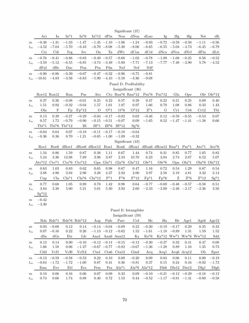
Significant (37)

Aci Ia Iaq1 Iaq6 Iaq12 dPia Noa dNoa dLno Ig 2Ig 3Ig Nsi dIi

m −0.38 −1.31 −1.33 −1.47 −1.45 −1.10 −1.06 −1.24 −0.93 −0.72 −0.58 −0.56 −1.11 −0.56tm −4.52 −7.04 −5.70 −6.43 −6.70 −8.08 −5.38 −8.06 −6.65 −6.55 −5.04 −4.73 −6.45 −6.79

Cei Cdi Ivg Ivc Oa Ta dWc dCoa dCol dNco dNca dNcl dFin dLti

m −0.76 −0.41 −0.86 −0.83 −0.49 −0.57 −0.68 −1.02 −0.78 −1.09 −1.08 −0.25 0.56 −0.52tm −3.59 −5.12 −6.55 −6.85 −3.74 −3.49 −5.80 −7.71 −7.13 −7.77 −7.48 −2.90 5.78 −4.52

dFnl dBe Dac Poa Pta Pda Nxf Nef Ndf

m −0.90 −0.86 −0.39 −0.67 −0.47 −0.32 −0.96 −0.75 −0.81tm −10.61 −4.83 −3.56 −6.83 −5.90 −4.10 −5.58 −3.36 −9.08

Panel D: Profitability

Insignificant (36)

Roe12 Roa12 Rna Pm Ato Cto Rnaq6 Rnaq12 Pmq6 Pmq12 Gla Ope Ole Oleq12

m 0.37 0.26 −0.08 −0.01 0.25 0.22 0.57 0.29 0.47 0.22 0.21 0.25 0.09 0.40tm 1.51 0.92 −0.32 −0.04 1.57 1.01 1.87 0.97 1.66 0.79 1.08 0.86 0.33 1.43

Ola F Fp Fpq12 O Oq1 Oq6 Oq12 Zq1 G Cr1 Cr6 Cr12 Tbi

m 0.13 0.39 −0.27 −0.29 −0.04 −0.17 −0.02 0.03 −0.46 0.12 −0.59 −0.55 −0.53 0.07tm 0.57 1.72 −0.79 −0.90 −0.15 −0.51 −0.07 0.09 −1.65 0.52 −1.47 −1.41 −1.38 0.66

Tbiq1 Tbiq6 Tbiq12 Bl Blq1 Blq6 Blq12 Sgq6

m −0.04 0.04 0.07 −0.18 −0.11 −0.17 −0.18 −0.04tm −0.36 0.36 0.70 −1.21 −0.65 −1.00 −1.09 −0.32

Significant (43)

Roe1 Roe6 dRoe1 dRoe6 dRoe12 Roa1 Roa6 dRoa1 dRoa6 dRoa12 Rnaq1 Pmq1 Atoq1 Atoq6

m 1.34 0.86 1.59 0.87 0.38 1.11 0.67 1.44 0.74 0.31 0.85 0.77 1.05 0.82tm 5.24 3.36 12.08 7.89 3.96 3.87 2.33 10.70 6.23 3.04 2.74 2.67 6.52 5.07

Atoq12 Ctoq1 Ctoq6 Ctoq12 Gpa Glaq1 Glaq6 Glaq12 Oleq1 Oleq6 Opa Olaq1 Olaq6 Olaq12

m 0.63 1.03 0.83 0.62 0.65 0.98 0.67 0.47 1.16 0.72 0.54 1.29 0.87 0.54tm 3.88 4.90 3.94 2.96 3.28 4.37 2.92 2.00 3.97 2.58 2.19 4.81 3.32 2.14

Cop Cla Claq1 Claq6 Claq12 Fq1 Fq6 Fq12 Fpq1 Fpq6 Z Zq6 Zq12 Sgq1

m 0.77 0.68 1.05 0.89 0.78 1.42 0.98 0.64 −0.77 −0.69 −0.48 −0.57 −0.58 0.51tm 3.84 3.38 5.60 5.21 5.01 5.30 3.92 2.60 −2.33 −2.09 −2.48 −2.17 −2.36 3.50

Sgq12

m −0.42tm −3.30

Panel E: Intangibles

Insignificant (59)

Rds Rdsq1 Rdsq6 Rdsq12 Aop Pafe Parc Crd Hs Ha He Age1 Age6 Age12

m 0.03 −0.08 0.12 0.14 −0.14 −0.04 −0.09 0.22 −0.20 −0.19 −0.17 0.29 0.35 0.33tm 0.07 −0.16 0.22 0.26 −1.13 −0.12 −0.62 1.52 −1.61 −1.18 −0.89 1.31 1.59 1.52

dSa dGs Etr Lfe Ana1 Ana6 Ana12 Kz Kzq6 Kzq12 Wwq1 Wwq6 Wwq12 Sdd

m 0.12 0.14 0.00 −0.10 −0.12 −0.14 −0.15 −0.12 −0.30 −0.27 0.32 0.41 0.47 0.08tm 1.66 1.58 0.06 −1.27 −0.67 −0.77 −0.82 −0.67 −1.36 −1.28 0.89 1.16 1.35 0.73

Cdd Vcf1 Vcf6 Vcf12 Cta1 Cta6 Cta12 Gind Acq Acq1 Acq6 Acq12 Ob Eper

m −0.13 −0.59 −0.58 −0.53 0.22 0.10 0.09 −0.20 0.09 0.04 0.06 0.11 0.00 −0.19tm −0.64 −1.72 −1.72 −1.60 0.87 0.41 0.36 −0.81 0.37 0.15 0.24 0.44 −0.02 −1.73

Esm Evr Etl Ecs Frm Fra Alaq1 Alaq6 Alaq12 Dls6 Dls12 Dis12 Dlg1 Dlg6

m 0.10 0.06 0.16 0.06 0.07 0.09 0.33 0.09 −0.10 −0.21 −0.12 −0.29 −0.18 −0.12tm 0.74 0.66 1.74 0.88 0.40 0.72 1.53 0.44 −0.52 −1.17 −0.81 −1.41 −0.80 −0.58

70

Dlg12 R1n R

[11,15]n

m −0.11 −0.36 −0.24tm −0.53 −1.05 −1.76

Significant (44)

Oca Ioca Adm gAd Rdm Rdmq1 Rdmq6 Rdmq12 Ol Olq1 Olq6 Olq12 Hn Rca

m 0.78 0.74 0.97 −0.66 1.89 3.43 2.69 2.62 0.58 0.69 0.65 0.60 −0.86 0.89tm 3.52 5.18 3.59 −4.30 5.64 5.99 5.26 5.72 3.21 3.54 3.34 3.11 −6.26 2.02

Bca D1 D2 D3 dSi dSs Tan Tanq1 Tanq6 Tanq12 Rer Kzq1 Ww Eprd

m 0.37 1.02 1.11 1.09 0.15 −0.22 0.49 0.78 0.71 0.59 0.23 −0.51 0.72 −0.72tm 2.09 3.78 3.86 3.80 2.10 −2.26 2.82 4.35 4.00 3.42 2.11 −2.13 2.15 −3.88

Ala Alm Almq1 Almq6 Almq12 Dls1 Dis1 Dis6 R1a R

[2,5]a R

[2,5]n R

[6,10]a R

[6,10]n R

[11,15]a

m −0.65 0.36 1.59 1.48 1.30 −0.64 −0.67 −0.46 0.77 0.85 −1.43 0.82 −0.67 0.70tm −4.31 2.29 7.09 7.04 6.40 −3.31 −2.99 −2.11 4.96 5.92 −6.25 6.05 −4.61 6.19

R[16,20]a R

[16,20]n

m 0.61 −0.30tm 5.18 −2.50

Panel F: Trading frictions

Insignificant (62)

Iv Ivff1 Ivff6 Ivff12 Ivc1 Ivc6 Ivc12 Ivq1 Ivq6 Ivq12 Tv1 Tv6 Tv12 Sv6

m 0.31 −0.27 −0.03 0.16 −0.28 −0.03 0.15 −0.28 −0.04 0.14 −0.28 −0.04 0.13 −0.11tm 0.75 −0.75 −0.09 0.45 −0.78 −0.09 0.44 −0.79 −0.12 0.41 −0.76 −0.11 0.37 −1.63

Sv12 β1 β6 β12 βFP1 βFP6 βFP12 βD6 Cvd1 Lm11 Mdr6 Mdr12 Ts6 Ts12

m −0.07 −0.08 −0.06 −0.11 −0.47 −0.38 −0.33 −0.23 0.36 0.44 −0.17 0.03 −0.02 0.03tm −1.19 −0.27 −0.21 −0.38 −1.40 −1.17 −1.07 −1.96 1.92 1.89 −0.54 0.09 −0.22 0.40

Isc6 Isc12 Isff6 Isff12 Isq6 Isq12 Cs1 Cs6 Cs12 Tail1 Tail6 βret1 βret6 βret12

m −0.01 0.03 0.01 0.04 0.01 0.04 −0.04 0.00 0.00 0.20 0.29 −0.12 −0.11 −0.15tm −0.15 0.46 0.16 0.69 0.16 0.63 −0.54 −0.01 −0.11 1.11 1.88 −0.40 −0.38 −0.54

βlcc1 βlcc6 βlcc12 βlrc1 βlrc6 βlrc12 βlcr1 βlcr6 βlcr12 βnet1 βnet6 βnet12 Shl1 Shl6

m 0.30 0.29 0.27 −0.02 −0.06 −0.02 0.03 0.00 0.00 0.13 0.05 −0.00 0.64 0.63tm 1.63 1.64 1.59 −0.06 −0.25 −0.08 0.26 0.03 0.01 0.47 0.18 −0.02 1.84 1.93

Sba1 Sba6 Sba12 βlev1 βlev6 βlev12

m 0.50 0.59 0.59 0.35 0.24 0.16tm 1.19 1.55 1.63 1.85 1.40 0.98

Significant (40)

Me Sv1 βD1 βD12 Tur1 Tur6 Tur12 Cvt1 Cvt6 Cvt12 Dtv1 Dtv6 Dtv12 Cvd6

m −1.20 −0.36 −0.45 −0.26 −0.85 −0.97 −0.95 0.43 0.50 0.54 −1.19 −1.20 −1.21 0.48tm −4.01 −2.37 −2.62 −2.44 −3.39 −4.02 −4.06 2.57 3.07 3.47 −4.73 −4.90 −5.04 2.68

Cvd12 Pps1 Pps6 Pps12 Ami1 Ami6 Ami12 Lm16 Lm112 Lm61 Lm66 Lm612 Lm121 Lm126

m 0.52 −1.44 −1.01 −1.02 1.06 1.17 1.21 1.00 1.04 1.20 1.23 1.16 1.20 1.17tm 3.06 −3.53 −2.57 −2.72 3.52 3.93 4.12 4.50 4.89 5.02 5.36 5.27 5.09 5.18

Lm1212 Mdr1 Ts1 Isc1 Isff1 Isq1 Srev β−1 β−6 β−12 Tail12 Shl12

m 1.09 −0.73 −0.46 −0.38 −0.24 −0.23 −2.65 −0.80 −0.96 −0.79 0.33 0.73tm 5.00 −2.29 −3.95 −3.48 −2.40 −2.45 −9.22 −2.79 −3.49 −3.02 2.31 2.34

71

Table 7 : Portfolio Weights on Microcaps and Investment Capacity, January 1967 toDecember 2014, 576 Months

The six categories of anomalies, momentum, value-versus-growth, investment, profitability,intangibles, and trading frictions are denoted by Mom, VvG, Inv, Prof, Intan, and Fric, respectively.In Panel A, we calculate the time series average of portfolio weights on microcaps for the low andhigh deciles of each anomaly variable, and then report the average across all the anomalies withina given category. In Panel B, the investment capacity of a portfolio is defined as mini{Mei/wi},in which Mei is the market equity of stock i, and wi is its portfolio weight. For the low and highdeciles of each anomaly variable, we calculate the investment capacity at each month, take timeseries average, and then report the average across all the anomalies within a given category.

Mom VvG Inv Prof Intan Fric

Panel A: Portfolio weights (in percent) allocated to microcaps

NYSE breakpoints and value-weights

Low 7.34 4.04 7.58 9.65 4.09 10.50High 3.50 7.56 5.69 5.98 10.43 20.53

NYSE-Amex-NASDAQ breakpoints and equal-weights

Low 64.19 51.88 71.67 68.90 47.97 55.12High 49.06 64.86 60.89 55.31 62.54 73.65

Panel B: Investment capacity as a fraction of the total market equity (in percent)

NYSE breakpoints and value-weights

Low 7.119 13.394 5.886 8.553 9.900 15.676High 10.342 5.697 7.487 11.162 8.662 8.807

NYSE-Amex-NASDAQ breakpoints and equal-weights

Low 0.016 0.028 0.012 0.029 0.181 0.207High 0.027 0.015 0.017 0.019 0.046 0.185

72

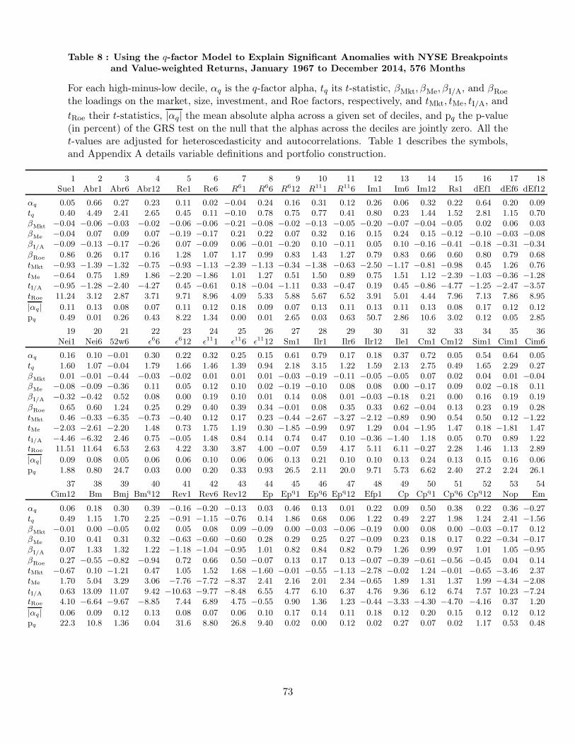
Table 8 : Using the q-factor Model to Explain Significant Anomalies with NYSE Breakpointsand Value-weighted Returns, January 1967 to December 2014, 576 Months

For each high-minus-low decile, αq is the q-factor alpha, tq its t-statistic, βMkt, βMe, βI/A, and βRoe

the loadings on the market, size, investment, and Roe factors, respectively, and tMkt, tMe, tI/A, and

tRoe their t-statistics, |αq| the mean absolute alpha across a given set of deciles, and pq the p-value(in percent) of the GRS test on the null that the alphas across the deciles are jointly zero. All thet-values are adjusted for heteroscedasticity and autocorrelations. Table 1 describes the symbols,and Appendix A details variable definitions and portfolio construction.

1 2 3 4 5 6 7 8 9 10 11 12 13 14 15 16 17 18Sue1 Abr1 Abr6 Abr12 Re1 Re6 R61 R66 R612 R111 R116 Im1 Im6 Im12 Rs1 dEf1 dEf6 dEf12

αq 0.05 0.66 0.27 0.23 0.11 0.02 −0.04 0.24 0.16 0.31 0.12 0.26 0.06 0.32 0.22 0.64 0.20 0.09tq 0.40 4.49 2.41 2.65 0.45 0.11 −0.10 0.78 0.75 0.77 0.41 0.80 0.23 1.44 1.52 2.81 1.15 0.70βMkt −0.04 −0.06 −0.03 −0.02 −0.06 −0.06 −0.21 −0.08 −0.02 −0.13 −0.05 −0.20 −0.07 −0.04 −0.05 0.02 0.06 0.03βMe −0.04 0.07 0.09 0.07 −0.19 −0.17 0.21 0.22 0.07 0.32 0.16 0.15 0.24 0.15 −0.12 −0.10 −0.03 −0.08βI/A −0.09 −0.13 −0.17 −0.26 0.07 −0.09 0.06 −0.01 −0.20 0.10 −0.11 0.05 0.10 −0.16 −0.41 −0.18 −0.31 −0.34

βRoe 0.86 0.26 0.17 0.16 1.28 1.07 1.17 0.99 0.83 1.43 1.27 0.79 0.83 0.66 0.60 0.80 0.79 0.68tMkt −0.93 −1.39 −1.32 −0.75 −0.93 −1.13 −2.39 −1.13 −0.34 −1.38 −0.63 −2.50 −1.17 −0.81 −0.98 0.45 1.26 0.76tMe −0.64 0.75 1.89 1.86 −2.20 −1.86 1.01 1.27 0.51 1.50 0.89 0.75 1.51 1.12 −2.39 −1.03 −0.36 −1.28tI/A −0.95 −1.28 −2.40 −4.27 0.45 −0.61 0.18 −0.04 −1.11 0.33 −0.47 0.19 0.45 −0.86 −4.77 −1.25 −2.47 −3.57tRoe 11.24 3.12 2.87 3.71 9.71 8.96 4.09 5.33 5.88 5.67 6.52 3.91 5.01 4.44 7.96 7.13 7.86 8.95

|αq| 0.11 0.13 0.08 0.07 0.11 0.12 0.18 0.09 0.07 0.13 0.11 0.13 0.11 0.13 0.08 0.17 0.12 0.12pq 0.49 0.01 0.26 0.43 8.22 1.34 0.00 0.01 2.65 0.03 0.63 50.7 2.86 10.6 3.02 0.12 0.05 2.85

19 20 21 22 23 24 25 26 27 28 29 30 31 32 33 34 35 36Nei1 Nei6 52w6 ǫ66 ǫ612 ǫ111 ǫ116 ǫ1112 Sm1 Ilr1 Ilr6 Ilr12 Ile1 Cm1 Cm12 Sim1 Cim1 Cim6

αq 0.16 0.10 −0.01 0.30 0.22 0.32 0.25 0.15 0.61 0.79 0.17 0.18 0.37 0.72 0.05 0.54 0.64 0.05tq 1.60 1.07 −0.04 1.79 1.66 1.46 1.39 0.94 2.18 3.15 1.22 1.59 2.13 2.75 0.49 1.65 2.29 0.27βMkt 0.01 −0.01 −0.44 −0.03 −0.02 0.01 0.01 0.01 −0.03 −0.19 −0.11 −0.05 −0.05 0.07 0.02 0.04 0.01 −0.04βMe −0.08 −0.09 −0.36 0.11 0.05 0.12 0.10 0.02 −0.19 −0.10 0.08 0.08 0.00 −0.17 0.09 0.02 −0.18 0.11βI/A −0.32 −0.42 0.52 0.08 0.00 0.19 0.10 0.01 0.14 0.08 0.01 −0.03 −0.18 0.21 0.00 0.16 0.19 0.19

βRoe 0.65 0.60 1.24 0.25 0.29 0.40 0.39 0.34 −0.01 0.08 0.35 0.33 0.62 −0.04 0.13 0.23 0.19 0.28tMkt 0.46 −0.33 −6.35 −0.73 −0.40 0.12 0.17 0.23 −0.44 −2.67 −3.27 −2.12 −0.89 0.90 0.54 0.50 0.12 −1.22tMe −2.03 −2.61 −2.20 1.48 0.73 1.75 1.19 0.30 −1.85 −0.99 0.97 1.29 0.04 −1.95 1.47 0.18 −1.81 1.47tI/A −4.46 −6.32 2.46 0.75 −0.05 1.48 0.84 0.14 0.74 0.47 0.10 −0.36 −1.40 1.18 0.05 0.70 0.89 1.22tRoe 11.51 11.64 6.53 2.63 4.22 3.30 3.87 4.00 −0.07 0.59 4.17 5.11 6.11 −0.27 2.28 1.46 1.13 2.89

|αq| 0.09 0.08 0.05 0.06 0.06 0.10 0.06 0.06 0.13 0.21 0.10 0.10 0.13 0.24 0.13 0.15 0.16 0.06pq 1.88 0.80 24.7 0.03 0.00 0.20 0.33 0.93 26.5 2.11 20.0 9.71 5.73 6.62 2.40 27.2 2.24 26.1

37 38 39 40 41 42 43 44 45 46 47 48 49 50 51 52 53 54Cim12 Bm Bmj Bmq12 Rev1 Rev6 Rev12 Ep Epq1 Epq6 Epq12 Efp1 Cp Cpq1 Cpq6 Cpq12 Nop Em

αq 0.06 0.18 0.30 0.39 −0.16 −0.20 −0.13 0.03 0.46 0.13 0.01 0.22 0.09 0.50 0.38 0.22 0.36 −0.27tq 0.49 1.15 1.70 2.25 −0.91 −1.15 −0.76 0.14 1.86 0.68 0.06 1.22 0.49 2.27 1.98 1.24 2.41 −1.56βMkt −0.01 0.00 −0.05 0.02 0.05 0.08 0.09 −0.09 0.00 −0.03 −0.06 −0.19 0.00 0.08 0.00 −0.03 −0.17 0.12βMe 0.10 0.41 0.31 0.32 −0.63 −0.60 −0.60 0.28 0.29 0.25 0.27 −0.09 0.23 0.18 0.17 0.22 −0.34 −0.17βI/A 0.07 1.33 1.32 1.22 −1.18 −1.04 −0.95 1.01 0.82 0.84 0.82 0.79 1.26 0.99 0.97 1.01 1.05 −0.95

βRoe 0.27 −0.55 −0.82 −0.94 0.72 0.66 0.50 −0.07 0.13 0.17 0.13 −0.07 −0.39 −0.61 −0.56 −0.45 0.04 0.14tMkt −0.67 0.10 −1.21 0.47 1.05 1.52 1.68 −1.60 −0.01 −0.55 −1.13 −2.78 −0.02 1.24 −0.01 −0.65 −3.46 2.37tMe 1.70 5.04 3.29 3.06 −7.76 −7.72 −8.37 2.41 2.16 2.01 2.34 −0.65 1.89 1.31 1.37 1.99 −4.34 −2.08tI/A 0.63 13.09 11.07 9.42 −10.63 −9.77 −8.48 6.55 4.77 6.10 6.37 4.76 9.36 6.12 6.74 7.57 10.23 −7.24tRoe 4.10 −6.64 −9.67 −8.85 7.44 6.89 4.75 −0.55 0.90 1.36 1.23 −0.44 −3.33 −4.30 −4.70 −4.16 0.37 1.20

|αq| 0.06 0.09 0.12 0.13 0.08 0.07 0.06 0.10 0.17 0.14 0.11 0.18 0.12 0.20 0.15 0.12 0.12 0.12pq 22.3 10.8 1.36 0.04 31.6 8.80 26.8 9.40 0.02 0.00 0.12 0.02 0.27 0.07 0.02 1.17 0.53 0.48

73

55 56 57 58 59 60 61 62 63 64 65 66 67 68 69 70 71 72Emq1 Emq6 Emq12 Sp Spq1 Spq6 Spq12 Ocp Ocpq1 Ir Vhp Vfp Ebp Dur Aci I/A Iaq6 Iaq12

αq −0.63 −0.34 −0.30 −0.04 0.21 0.15 0.06 0.41 0.46 −0.18 −0.01 0.22 0.09 −0.10 −0.17 0.07 −0.11 0.00tq −2.55 −1.59 −1.55 −0.19 0.70 0.59 0.28 2.25 1.47 −1.13 −0.05 0.95 0.66 −0.53 −1.05 0.61 −0.96 0.04βMkt 0.07 0.09 0.11 0.09 0.13 0.09 0.07 −0.02 0.11 −0.03 −0.04 −0.05 0.05 0.07 0.01 0.03 0.07 0.04βMe 0.02 −0.02 −0.07 0.62 0.59 0.61 0.64 0.16 0.13 −0.57 0.24 0.15 0.51 −0.27 −0.29 −0.13 −0.18 −0.21βI/A −0.67 −0.67 −0.71 1.14 1.07 1.11 1.08 1.37 1.19 −1.16 0.91 0.50 1.19 −0.97 0.13 −1.37 −1.35 −1.36

βRoe 0.03 0.03 −0.01 −0.30 −0.56 −0.51 −0.39 −0.50 −0.58 0.65 −0.10 0.18 −0.59 0.18 −0.20 0.16 0.34 0.21tMkt 1.26 1.77 2.33 1.77 1.88 1.47 1.31 −0.33 1.23 −0.64 −0.62 −0.84 1.01 1.14 0.18 1.06 2.23 1.41tMe 0.19 −0.18 −0.76 4.50 3.43 3.98 4.54 1.40 0.64 −7.94 2.01 1.46 6.51 −1.97 −4.98 −2.31 −3.30 −4.28tI/A −4.56 −5.53 −5.95 9.49 5.92 7.02 7.99 9.73 5.54 −10.70 5.82 3.04 12.49 −6.69 1.04 −16.72 −12.31 −13.62tRoe 0.25 0.23 −0.09 −2.87 −3.13 −3.37 −3.20 −4.31 −2.96 7.39 −0.78 1.51 −7.49 1.42 −2.26 2.54 4.37 3.11

|αq | 0.23 0.15 0.13 0.06 0.08 0.07 0.07 0.11 0.19 0.07 0.14 0.15 0.12 0.08 0.13 0.09 0.07 0.06pq 0.00 0.16 0.05 27.4 32.0 40.7 21.5 2.74 27.6 43.8 1.28 6.23 0.40 42.0 0.17 0.02 5.33 14.3

73 74 75 76 77 78 79 80 81 82 83 84 85 86 87 88 89 90dPia Noa dNoa dLno Ig 2Ig Nsi dIi Cei Ivg Ivc Oa dWc dCoa dNco dNca dFin dFnl

αq −0.22 −0.41 −0.10 0.03 −0.03 0.05 −0.29 0.12 −0.24 0.01 −0.30 −0.54 −0.48 0.12 −0.03 0.00 0.44 −0.08tq −1.77 −2.24 −0.66 0.16 −0.27 0.42 −2.19 1.14 −1.85 0.11 −2.11 −3.77 −3.43 1.16 −0.23 0.03 2.94 −0.73βMkt 0.04 −0.01 0.00 −0.08 −0.02 0.07 0.04 0.03 0.22 −0.02 0.05 0.06 0.03 0.05 −0.02 −0.05 −0.03 0.03βMe −0.09 0.11 0.03 −0.16 −0.15 −0.30 0.15 −0.17 0.28 0.07 0.00 0.31 0.35 −0.04 −0.08 −0.10 −0.11 −0.06βI/A −0.82 −0.07 −1.05 −0.81 −0.75 −0.73 −0.67 −0.64 −1.04 −0.94 −0.67 −0.02 −0.33 −1.15 −0.78 −0.87 −0.30 −0.42

βRoe 0.14 0.00 0.02 0.02 −0.06 −0.07 −0.28 −0.21 −0.12 0.04 0.20 0.26 0.14 0.13 0.00 0.03 0.03 −0.14tMkt 1.14 −0.14 −0.11 −1.60 −0.70 1.88 1.07 1.01 6.28 −0.66 1.44 1.83 0.62 1.97 −0.59 −1.42 −1.08 1.00tMe −1.86 1.04 0.55 −2.34 −2.64 −4.76 2.15 −3.68 4.25 1.70 −0.08 5.06 4.32 −0.85 −1.61 −1.94 −2.19 −1.50tI/A −8.63 −0.44 −9.49 −6.86 −10.47 −9.36 −7.67 −7.58 −13.74 −12.85 −6.21 −0.23 −3.20 −16.21 −10.85 −11.77 −2.54 −5.58tRoe 1.83 0.04 0.25 0.15 −0.90 −1.01 −4.39 −2.99 −1.57 0.59 2.26 4.13 2.18 2.10 0.00 0.41 0.45 −2.05

|αq | 0.12 0.11 0.07 0.05 0.09 0.08 0.11 0.07 0.12 0.10 0.08 0.13 0.13 0.08 0.10 0.10 0.08 0.09pq 0.22 0.06 20.9 61.8 1.22 7.65 0.10 41.8 0.44 6.74 27.2 0.03 0.04 6.16 0.39 1.09 2.46 4.83

91 92 93 94 95 96 97 98 99 100 101 102 103 104 105 106 107 108Dac Poa Pta Pda Ndf Roe1 dRoe1 dRoe6 dRoe12 Roa1 dRoa1 dRoa6 Rnaq1 Atoq1 Atoq6 Atoq12 Ctoq1 Ctoq6

αq −0.64 −0.07 −0.15 −0.28 0.03 −0.03 0.34 −0.02 −0.09 0.04 0.06 −0.18 0.18 0.31 0.32 0.30 −0.11 −0.08tq −4.37 −0.57 −1.07 −1.88 0.25 −0.27 2.29 −0.20 −0.96 0.31 0.36 −1.23 1.32 1.75 1.88 1.85 −0.65 −0.48βMkt 0.01 −0.01 0.06 0.05 0.06 −0.08 0.03 0.04 0.01 −0.13 0.11 0.09 −0.14 0.11 0.09 0.08 0.12 0.12βMe 0.19 0.14 0.17 0.05 −0.12 −0.37 −0.06 −0.02 −0.01 −0.37 0.09 0.11 −0.44 0.43 0.38 0.33 0.33 0.32βI/A 0.23 −0.94 −0.87 −0.18 −0.44 0.12 0.23 0.21 0.14 −0.08 0.25 0.19 −0.14 −0.49 −0.61 −0.69 −0.14 −0.21

βRoe 0.19 0.07 0.05 −0.09 −0.26 1.49 0.58 0.56 0.52 1.34 0.59 0.59 1.29 0.55 0.53 0.47 0.83 0.77tMkt 0.32 −0.35 1.69 1.32 1.76 −2.22 0.64 0.97 0.26 −4.17 2.44 1.96 −3.48 1.87 1.69 1.52 2.08 2.29tMe 3.27 3.36 2.66 0.63 −2.34 −6.34 −0.88 −0.42 −0.16 −6.34 1.30 1.59 −8.60 5.44 5.41 5.64 3.03 3.34tI/A 2.38 −11.07 −8.94 −1.34 −5.80 1.24 2.75 2.60 2.53 −0.95 2.15 2.13 −1.40 −4.70 −5.95 −6.82 −1.31 −2.04tRoe 3.05 1.39 0.65 −0.97 −3.79 19.40 6.76 6.02 8.01 17.49 5.18 5.51 19.43 5.73 7.03 6.73 10.37 10.61

|αq | 0.15 0.12 0.08 0.17 0.08 0.10 0.09 0.07 0.08 0.06 0.10 0.08 0.07 0.11 0.07 0.08 0.09 0.09pq 0.01 0.08 4.22 0.00 36.2 0.63 4.31 4.84 0.77 85.3 42.1 4.25 22.5 3.39 14.3 9.13 24.5 1.39

74

109 110 111 112 113 114 115 116 117 118 119 120 121 122 123 124 125 126Ctoq12 Gpa Glaq1 Glaq6 Glaq12 Oleq1 Oleq6 Olaq1 Olaq6 Olaq12 Cop Cla Claq1 Claq6 Claq12 Fq1 Fq6 Fq12

αq −0.05 0.18 0.20 0.10 0.13 −0.04 −0.16 0.37 0.25 0.33 0.69 0.74 0.43 0.40 0.46 0.13 0.15 0.07tq −0.31 1.24 1.41 0.79 1.01 −0.25 −1.06 2.34 1.78 2.48 4.77 4.89 2.69 2.82 3.56 0.58 0.86 0.49βMkt 0.11 0.04 0.00 0.02 0.01 −0.05 −0.06 −0.11 −0.10 −0.13 −0.23 −0.21 −0.08 −0.04 −0.07 −0.07 −0.03 −0.05βMe 0.30 0.03 0.11 0.06 0.05 −0.24 −0.29 −0.33 −0.37 −0.37 −0.60 −0.62 −0.32 −0.32 −0.31 −0.33 −0.40 −0.41βI/A −0.27 −0.31 −0.28 −0.37 −0.45 0.38 0.33 −0.24 −0.31 −0.42 −0.06 −0.31 −0.13 −0.13 −0.19 0.44 0.33 0.32

βRoe 0.72 0.55 0.66 0.60 0.53 1.15 1.05 1.08 0.98 0.89 0.49 0.40 0.48 0.45 0.40 0.73 0.67 0.65tMkt 2.06 0.95 −0.10 0.82 0.23 −1.08 −1.43 −2.44 −3.08 −4.28 −5.84 −5.46 −1.87 −1.46 −2.79 −1.03 −0.70 −0.99tMe 3.48 0.69 2.20 1.23 1.11 −2.25 −3.31 −3.82 −5.62 −5.68 −7.78 −8.65 −4.77 −5.77 −6.01 −3.16 −4.55 −4.82tI/A −2.68 −3.21 −3.03 −4.56 −5.22 2.63 2.64 −2.09 −3.25 −4.60 −0.66 −3.35 −1.07 −1.24 −2.14 3.07 2.80 3.18tRoe 10.25 7.66 12.26 10.83 8.96 10.91 9.99 13.43 14.45 12.18 7.88 6.00 5.25 7.12 7.34 6.97 6.90 7.11

|αq | 0.09 0.12 0.11 0.11 0.10 0.07 0.09 0.12 0.08 0.08 0.17 0.14 0.18 0.10 0.11 0.10 0.15 0.11pq 0.62 10.7 11.6 20.2 41.4 8.56 0.82 0.82 2.91 4.49 0.00 0.00 0.03 5.14 0.04 10.2 0.01 0.09

127 128 129 130 131 132 133 134 135 136 137 138 139 140 141 142 143 144Fpq6 Tbiq12 Oca Ioca Adm Rdm Rdmq1 Rdmq6 Rdmq12 Ol Olq1 Olq6 Olq12 Hs Etr Rer Eprd Etl

αq −0.17 0.34 0.13 0.07 0.08 0.70 1.47 0.97 0.80 0.03 0.07 0.09 0.12 −0.31 0.09 0.39 −0.49 0.28tq −0.63 2.93 0.65 0.53 0.31 2.89 2.97 2.73 2.80 0.19 0.37 0.54 0.69 −1.51 0.69 2.20 −2.77 1.55βMkt 0.41 −0.07 −0.16 −0.06 0.07 0.16 0.01 −0.08 −0.08 −0.04 −0.10 −0.13 −0.13 −0.17 0.01 0.05 0.10 0.01βMe 0.40 −0.17 0.22 0.25 0.48 0.62 0.14 0.52 0.62 0.30 0.27 0.32 0.32 −0.08 0.12 −0.13 0.35 0.29βI/A 0.10 −0.14 0.27 0.36 1.36 0.17 0.61 0.69 0.82 0.11 0.04 0.05 0.04 0.28 0.04 −0.15 0.41 −0.13

βRoe −1.54 0.05 0.55 0.51 −0.30 −0.62 −1.02 −0.90 −0.70 0.55 0.67 0.62 0.59 −0.03 0.18 0.01 −0.62 0.05tMkt 5.87 −2.10 −2.41 −1.88 0.76 2.45 0.05 −0.96 −1.04 −0.80 −1.84 −2.66 −2.85 −3.35 0.36 0.93 1.63 0.25tMe 2.19 −3.37 2.89 5.60 2.75 6.37 0.71 3.56 4.72 3.18 3.34 3.64 4.03 −0.96 2.19 −1.28 4.21 3.18tI/A 0.39 −2.07 2.05 3.73 5.94 0.95 1.99 3.17 4.35 0.95 0.33 0.38 0.34 1.69 0.40 −1.17 3.59 −0.87tRoe −8.64 0.65 4.38 7.32 −1.49 −4.26 −3.50 −4.82 −4.62 5.07 6.80 5.82 5.75 −0.21 2.29 0.10 −6.46 0.54

|αq | 0.12 0.10 0.12 0.10 0.07 0.27 0.55 0.49 0.47 0.11 0.09 0.09 0.09 0.14 0.10 0.15 0.17 0.08pq 0.04 0.00 4.95 1.18 69.1 0.05 0.00 0.00 0.00 2.57 15.3 2.77 1.04 3.05 1.86 2.06 0.62 22.7

145 146 147 148 149 150 151 152 153 154 155 156 157 158 159 160 161

Almq1 Almq6 Almq12 R1a R

[2,5]a R

[2,5]n R

[6,10]a R

[6,10]n R

[11,15]a R

[16,20]a Sv1 Dtv6 Dtv12 Ami12 Ts1 Isff1 Isq1

αq 0.28 0.25 0.15 0.55 0.81 −0.16 1.13 0.07 0.65 0.64 −0.35 −0.11 −0.13 0.15 0.31 0.31 0.31tq 1.77 1.78 1.08 2.48 3.90 −0.86 4.88 0.35 3.60 3.14 −1.42 −1.21 −1.65 2.03 2.75 2.64 3.01βMkt 0.07 0.06 0.07 0.23 0.06 0.19 −0.03 0.16 −0.01 −0.07 0.04 0.14 0.13 −0.03 0.03 −0.01 −0.02βMe 0.67 0.71 0.72 −0.14 −0.18 −0.27 0.03 −0.31 −0.07 −0.07 0.35 −1.08 −1.14 1.30 0.06 0.17 0.19βI/A 0.83 0.77 0.70 −0.15 −0.28 −1.32 −0.37 −0.81 −0.03 −0.04 −0.14 −0.38 −0.36 0.15 −0.08 0.01 −0.06

βRoe −0.44 −0.33 −0.24 0.18 0.05 0.38 −0.23 −0.28 0.10 0.00 −0.44 0.33 0.29 −0.36 −0.15 −0.04 −0.13tMkt 1.83 2.04 2.23 4.14 1.06 3.03 −0.64 3.06 −0.25 −1.37 0.65 4.54 5.12 −1.14 1.13 −0.27 −0.66tMe 7.56 10.54 11.47 −1.28 −1.75 −2.08 0.31 −3.40 −0.83 −1.21 2.58 −17.69 −31.71 42.18 1.41 4.25 2.54tI/A 8.07 9.20 8.45 −0.97 −2.46 −9.56 −2.22 −5.88 −0.23 −0.34 −0.80 −5.64 −7.11 2.95 −0.83 0.13 −0.74tRoe −5.96 −5.55 −3.73 1.25 0.47 2.77 −1.97 −2.30 1.09 −0.01 −3.45 6.94 7.17 −8.56 −3.04 −0.77 −2.40

|αq | 0.09 0.10 0.07 0.15 0.17 0.13 0.24 0.15 0.18 0.17 0.12 0.08 0.09 0.12 0.10 0.10 0.11pq 7.29 4.37 21.9 9.37 0.01 0.03 0.00 0.34 0.05 0.57 4.77 0.01 0.06 0.01 0.95 0.26 0.22

75

Table 9 : Pairwise Cross-sectional Rank Correlations for q-anomailes, January 1967 to December 2014, 576 Months

The six categories of anomalies, including momentum, value-versus-growth, investment, profitability, intangibles, and trading frictionsare denoted by Mom, VvG, Inv, Prof, Intan, and Fric, respectively. Rank correlations are calculated with each anomaly variable’sNYSE percentile rankings in the cross section. Panel A reports average within-category correlations, which are averaged across allthe pairwise rank correlations within a category, as well as average cross-category rank correlations, which are averaged across allpossible pairwise ranking correlations across a given pair of categories. Panel B shows average within-category rank correlations foreach q-anomaly. Table 1 describes the symbols, and Appendix A details variable definitions.

Panel A: Average within-category and cross-category rank correlations

Mom VvG Inv Prof Intan Fric

Mom 0.13 0.00 0.01 0.05 0.00 0.02VvG 0.42 0.08 0.04 0.01 −0.01Inv 0.32 0.07 0.02 0.01Prof 0.39 0.02 −0.07Intan 0.07 0.02Fric 0.42

Panel B: Average within-category rank correlations for individual q-anomalies

Mom VvG Inv Prof Intan Fric

Abr1 0.17 Bmq12 0.37 Noa 0.29 dRoe1 0.02 Rdm 0.20 Ami12 0.06Abr6 0.21 Cpq1 0.53 Nsi 0.09 Olaq1 0.50 Rdmq1 0.22 Ts1 0.52Abr12 0.19 Cpq6 0.54 Ivc 0.37 Olaq12 0.53 Rdmq6 0.22 Isff1 0.56dEf1 0.10 Nop 0.23 Oa 0.41 Cop 0.47 Rdmq12 0.23 Isq1 0.54Sm1 0.12 Emq1 0.43 dWc 0.45 Cla 0.47 Rer 0.01Ilr1 0.14 Ocp 0.40 dFin 0.25 Claq1 0.40 Eprd −0.08Ile1 0.04 Dac 0.38 Claq6 0.50 R1

a −0.02

Cm1 0.07 Claq12 0.54 R[2,5]a −0.01

Cim1 0.12 Tbiq12 0.09 R[6,10]a 0.01

R[11,15]a 0.02

R[16,20]a 0.02

76

Figure 1 : Time Series Properties of Microcaps, 1967–2014

Microcaps are stocks that are smaller than the 20th percentile of market equity for NYSE stocks, small stocks are those bigger than the20th percentile but smaller than the NYSE median, and big stocks are those bigger than the NYSE median. Panel A shows the timeseries of the number of microcaps (blue solid line), small stocks (red dashed line), and big stocks (black dashdot line) as a fraction ofthe total number of stocks at NYSE, Amex, and NASDAQ. Panel B plots the time series of the total market capitalization of microcaps(blue solid line) and small stocks (red dashed line) as a percentage of total market equity. Finally, Panel C plots the breakpoints forthe 20th percentile of NYSE market equity (blue solid line) and the NYSE median (red dashed line) in millions of dollars.

Panel A: Number of stocks for a size groupas a fraction of the total number of stocks

Panel B: Total market equity for a sizegroup as a fraction of total market equity

Panel C: Size breakpoints, $million

1970 1980 1990 2000 20100

0.2

0.4

0.6

0.8

1970 1980 1990 2000 20100

0.02

0.04

0.06

0.08

0.1

1970 1980 1990 2000 20100

500

1000

1500

2000

2500

3000

77

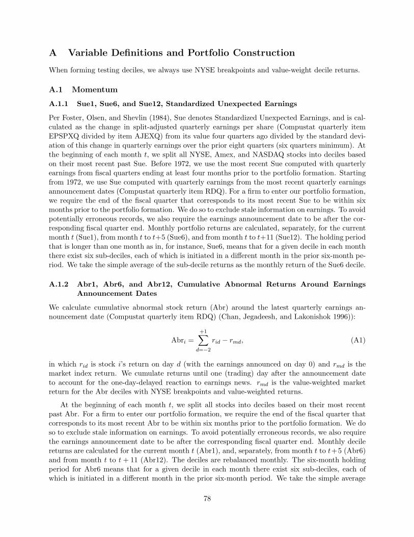
A Variable Definitions and Portfolio Construction

When forming testing deciles, we always use NYSE breakpoints and value-weight decile returns.

A.1 Momentum

A.1.1 Sue1, Sue6, and Sue12, Standardized Unexpected Earnings

Per Foster, Olsen, and Shevlin (1984), Sue denotes Standardized Unexpected Earnings, and is cal-culated as the change in split-adjusted quarterly earnings per share (Compustat quarterly itemEPSPXQ divided by item AJEXQ) from its value four quarters ago divided by the standard devi-ation of this change in quarterly earnings over the prior eight quarters (six quarters minimum). Atthe beginning of each month t, we split all NYSE, Amex, and NASDAQ stocks into deciles basedon their most recent past Sue. Before 1972, we use the most recent Sue computed with quarterlyearnings from fiscal quarters ending at least four months prior to the portfolio formation. Startingfrom 1972, we use Sue computed with quarterly earnings from the most recent quarterly earningsannouncement dates (Compustat quarterly item RDQ). For a firm to enter our portfolio formation,we require the end of the fiscal quarter that corresponds to its most recent Sue to be within sixmonths prior to the portfolio formation. We do so to exclude stale information on earnings. To avoidpotentially erroneous records, we also require the earnings announcement date to be after the cor-responding fiscal quarter end. Monthly portfolio returns are calculated, separately, for the currentmonth t (Sue1), from month t to t+5 (Sue6), and from month t to t+11 (Sue12). The holding periodthat is longer than one month as in, for instance, Sue6, means that for a given decile in each monththere exist six sub-deciles, each of which is initiated in a different month in the prior six-month pe-riod. We take the simple average of the sub-decile returns as the monthly return of the Sue6 decile.

A.1.2 Abr1, Abr6, and Abr12, Cumulative Abnormal Returns Around EarningsAnnouncement Dates

We calculate cumulative abnormal stock return (Abr) around the latest quarterly earnings an-nouncement date (Compustat quarterly item RDQ) (Chan, Jegadeesh, and Lakonishok 1996)):

Abri =

+1∑

d=−2

rid − rmd, (A1)

in which rid is stock i’s return on day d (with the earnings announced on day 0) and rmd is themarket index return. We cumulate returns until one (trading) day after the announcement dateto account for the one-day-delayed reaction to earnings news. rmd is the value-weighted marketreturn for the Abr deciles with NYSE breakpoints and value-weighted returns.

At the beginning of each month t, we split all stocks into deciles based on their most recentpast Abr. For a firm to enter our portfolio formation, we require the end of the fiscal quarter thatcorresponds to its most recent Abr to be within six months prior to the portfolio formation. We doso to exclude stale information on earnings. To avoid potentially erroneous records, we also requirethe earnings announcement date to be after the corresponding fiscal quarter end. Monthly decilereturns are calculated for the current month t (Abr1), and, separately, from month t to t+5 (Abr6)and from month t to t+ 11 (Abr12). The deciles are rebalanced monthly. The six-month holdingperiod for Abr6 means that for a given decile in each month there exist six sub-deciles, each ofwhich is initiated in a different month in the prior six-month period. We take the simple average

78

of the sub-decile returns as the monthly return of the Abr6 decile. Because quarterly earningsannouncement dates are largely unavailable before 1972, the Abr portfolios start in January 1972.

A.1.3 Re1, Re6, and Re12, Revisions in Analyst Earnings Forecasts

Following Chan, Jegadeesh, and Lakonishok (1996), we measure earnings surprise as the revisionsin analysts’ forecasts of earnings obtained from the Institutional Brokers’ Estimate System (IBES).Because analysts’ forecasts are not necessarily revised each month, we construct a six-month movingaverage of past changes in analysts’ forecasts:

REit =

6∑

τ=1

fit−τ − fit−τ−1

pit−τ−1, (A2)

in which fit−τ is the consensus mean forecast (IBES unadjusted file, item MEANEST) issued inmonth t − τ for firm i’s current fiscal year earnings (fiscal period indicator = 1), and pit−τ−1 isthe prior month’s share price (unadjusted file, item PRICE). We require both earnings forecastsand share prices to be denominated in US dollars (currency code = USD). We also adjust for anystock splits and require a minimum of four monthly forecast changes when constructing Re. Atthe beginning of each month t, we split all stocks into deciles based on their Re. Monthly decilereturns are calculated for the current month t (Re1), and, separately, from month t to t+ 5 (Re6)and from month t to t + 11 (Re12). The deciles are rebalanced monthly. The six-month holdingperiod for Re6 means that for a given decile in each month there exist six sub-deciles, each of whichis initiated in a different month in the prior six-month period. We take the simple average of thesub-decile returns as the monthly return of the Re6 decile. Because analyst forecast data start inJanuary 1976, the Re portfolios start in July 1976.

A.1.4 R61, R66, and R612, Prior Six-month Returns

At the beginning of each month t, we split all stocks into deciles based on their prior six-monthreturns from month t − 7 to t − 2. Skipping month t − 1, we calculate monthly decile returns,separately, for month t (R61), from month t to t + 5 (R66), and from month t to t + 11 (R612).The deciles are rebalanced at the beginning of month t+1. The holding period that is longer thanone month as in, for instance, R66, means that for a given decile in each month there exist sixsub-deciles, each of which is initiated in a different month in the prior six-month period. We takethe simple average of the sub-deciles returns as the monthly return of the R66 decile. We do notimpose a price screen to exclude stocks with prices per share below $5 as in Jegadeesh and Titman(1993). These stocks are mostly microcaps. Value-weighting returns assigns only tiny weights tothese stocks, which in turn do not need to be excluded.

A.1.5 R111, R116, and R1112, Prior 11-month Returns

We split all stocks into deciles at the beginning of each month t based on their prior 11-monthreturns from month t− 12 to t− 2. Skipping month t− 1, we calculate monthly decile returns formonth t (R111), from month t to t+5 (R116), and from month t to t+ 11 (R1112). All the decilesare rebalanced at the beginning of month t+ 1. The holding period that is longer than one monthas in, for instance, R116, means that for a given decile in each month there exist six subdeciles, eachof which is initiated in a different month in the prior six-month period. We take the simple average

79

of the subdecile returns as the monthly return of the R116 decile. Because we exclude financialfirms, these decile returns are different from those posted on Kenneth French’s Web site.

A.1.6 Im1, Im6, and Im12, Industry Momentum

We start with the FF 49-industry classifications. Excluding financial firms from the sample leaves45 industries. At the beginning of each month t, we sort industries based on their prior six-monthvalue-weighted returns from t−6 to t−1. Following Moskowitz and Grinblatt (1999), we do not skipmonth t− 1. We form nine portfolios (9× 5 = 45), each of which contains five different industries.We define the return of a given portfolio as the simple average of the five industry returns withinthe portfolio. We calculate portfolio returns for the nine portfolios for the current month t (Im1),from month t to t + 5 (Im6), and from month t to t + 11 (Im12). The portfolios are rebalancedat the beginning of t + 1. The holding period that is longer than one month as in, for instance,Im6, means that for a given portfolio in each month there exist six subportfolios, each of whichis initiated in a different month in the prior six-month period. We take the simple average of thesubportfolio returns as the monthly return of the Im6 portfolio.

A.1.7 Rs1, Rs6, and Rs12, Revenue Surprises

Following Jegadeesh and Livnat (2006), we measure revenue surprises (Rs) as changes in revenue pershare (Compustat quarterly item SALEQ/(item CSHPRQ times item AJEXQ)) from its value fourquarters ago divided by the standard deviation of this change in quarterly revenue per share over theprior eight quarters (six quarters minimum). At the beginning of each month t, we split stocks intodeciles based on their most recent past Rs. Before 1972, we use the most recent Rs computed withquarterly revenue from fiscal quarters ending at least four months prior to the portfolio formation.Starting from 1972, we use Rs computed with quarterly revenue from the most recent quarterlyearnings announcement dates (Compustat quarterly item RDQ). Jegadeesh and Livnat find thatquarterly revenue data are generally available when earnings are announced. For a firm to enterthe portfolio formation, we require the end of the fiscal quarter that corresponds to its most recentRs to be within six months prior to the portfolio formation. This restriction is imposed to excludestale revenue information. To avoid potentially erroneous records, we also require the earningsannouncement date to be after the corresponding fiscal quarter end. Monthly deciles returns arecalculated for the current month t (Rs1), from month t to t+ 5 (Rs6), and from month t to t+ 11(Rs12). The deciles are rebalanced at the beginning of month t + 1. The holding period that islonger than one month as in, for instance, Rs6, means that for a given decile in each month thereexist six subdeciles, each of which is initiated in a different month in the prior six-month period.We take the simple average of the subdeciles returns as the monthly return of the Rs6 decile.

A.1.8 Tes1, Tes6, and Tes12, Tax Expense Surprises

Following Thomas and Zhang (2011), we measure tax expense surprises (Tes) as changes in taxexpense, which is tax expense per share (Compustat quarterly item TXTQ/(item CSHPRQ timesitem AJEXQ)) in quarter q minus tax expense per share in quarter q − 4, scaled by assets pershare (item ATQ/(item CSHPRQ times item AJEXQ)) in quarter q − 4. At the beginning of eachmonth t, we sort stocks into deciles based on their Tes calculated with Compustat quarterly dataitems from at least four months ago. We exclude firms with zero Tes (most of these firms pay notaxes). We calculate decile returns the current month t (Tes1), from month t to t+ 5 (Tes6), andfrom month t to t+ 11 (Tes12). The deciles are rebalanced at the beginning of month t+ 1. The

80

holding period that is longer than one month as in, for instance, Tes6, means that for a given decilein each month there exist six subdeciles, each of which is initiated in a different month in the priorsix-month period. We take the simple average of the subdeciles returns as the monthly return ofthe Tes6 decile. For sufficient data coverage, we start the sample in January 1976.

A.1.9 dEf1, dEf6, and dEf12, Changes in Analyst Earnings Forecasts

Following Hawkins, Chamberlin, and Daniel (1984), we define dEf ≡ (fit−1 − fit−2)/(0.5 |fit−1| +0.5 |fit−2|), in which fit−1 is the consensus mean forecast (IBES unadjusted file, item MEANEST)issued in month t − 1 for firm i’s current fiscal year earnings (fiscal period indicator = 1). Werequire earnings forecasts to be denominated in US dollars (currency code = USD). We also adjustfor any stock splits between months t−2 and t−1 when constructing dEf. At the beginning of eachmonth t, we sort stocks into deciles on the prior month dEf, and calculate returns for the currentmonth t (dEf1), from month t to t + 5 (dEf6), and from month t to t + 11 (dEf12). The decilesare rebalanced at the beginning of month t+ 1. The holding period longer than one month as in,for instance, dEf6, means that for a given decile in each month there exist six subdeciles, each ofwhich is initiated in a different month in the prior six months. We take the simple average of thesubdecile returns as the monthly return of the dEf6 decile. Because analyst forecast data start inJanuary 1976, the dEf portfolios start in March 1976.

A.1.10 Nei1, Nei6, and Nei12, The Number of Quarters with Consecutive EarningsIncrease

We follow Barth, Elliott, and Finn (1999) and Green, Hand, and Zhang (2013) in measuring Nei asthe number of consecutive quarters (up to eight quarters) with an increase in earnings (Compustatquarterly item IBQ) over the same quarter in the prior year. At the beginning of each month t, wesort stocks into nine portfolios (with Nei = 0, 1, 2, . . . , 7, and 8, respectively) based on their mostrecent past Nei. Before 1972, we use Nei computed with quarterly earnings from fiscal quarters end-ing at least four months prior to the portfolio formation. Starting from 1972, we use Nei computedwith earnings from the most recent quarterly earnings announcement dates (Compustat quarterlyitem RDQ). For a firm to enter the portfolio formation, we require the end of the fiscal quarterthat corresponds to its most recent Nei to be within six months prior to the portfolio formation.This restriction is imposed to exclude stale earnings information. To avoid potentially erroneousrecords, we also require the earnings announcement date to be after the corresponding fiscal quarterend. We calculate monthly portfolio returns for the current month t (Nei1), from month t to t+ 5(Nei6), and from month t to t+ 11 (Nei12). The deciles are rebalanced at the beginning of montht+1. The holding period that is longer than one month as in, for instance, Nei6, means that for agiven decile in each month there exist six subdeciles, each of which is initiated in a different monthin the prior six-month period. We take the simple average of the subdeciles returns as the monthlyreturn of the Nei6 decile. For sufficient data coverage, the Nei portfolios start in January 1969.

A.1.11 52w1, 52w6, and 52w12, 52-week High

At the beginning of each month t, we split stocks into deciles based on 52w, which is the ratioof its split-adjusted price per share at the end of month t − 1 to its highest (daily) split-adjustedprice per share during the 12-month period ending on the last day of month t− 1. Monthly decilereturns are calculated for the current month t (52w1), from month t to t + 5 (52w6), and frommonth t to t + 11 (52w12), and the deciles are rebalanced at the beginning of month t + 1. The

81

holding period longer than one month as in 52w6 means that for a given decile in each month thereexist six subdeciles, each of which is initiated in a different month in the prior six months. We takethe simple average of the subdecile returns as the monthly return of the 52w6 decile. Because adisproportionately large number of stocks can reach the 52-week high at the same time and have52w equal to one, we use only 52w smaller than one to form the portfolio breakpoints. Doing sohelps avoid missing portfolio observations.

A.1.12 ǫ61, ǫ66, and ǫ612, Six-month Residual Momentum

We split all stocks into deciles at the beginning of each month t based on their prior six-monthaverage residual returns from month t− 7 to t− 2 scaled by their standard deviation over the sameperiod. Skipping month t− 1, we calculate monthly decile returns for month t (ǫ61), from month tto t+5 (ǫ66), and from month t to t+11 (ǫ612). Residual returns are estimated each month for allstocks over the prior 36 months from month t−36 to month t−1 from regressing stock excess returnson the Fama-French three factors. To reduce the noisiness of the estimation, we require returns tobe available for all prior 36 months. All the deciles are rebalanced at the beginning of month t+1.The holding period that is longer than 1 month as in ǫ66 means that for a given decile in eachmonth there exist six subdeciles, each of which is initiated in a different month in the prior six-monthperiod. We take the simple average of the subdecile returns as the monthly return of the ǫ66 decile.

A.1.13 ǫ111, ǫ116, and ǫ1112, 11-month Residual Momentum

We split all stocks into deciles at the beginning of each month t based on their prior 11-monthresidual returns from month t−12 to t−2 scaled by their standard deviation over the same period.Skipping month t−1, we calculate monthly decile returns for month t (ǫ111), from month t to t+5(ǫ116), and from month t to t+11 (ǫ1112). Residual returns are estimated each month for all stocksover the prior 36 months from month t− 36 to month t− 1 from regressing stock excess returns onthe Fama-French three factors. To reduce the noisiness of the estimation, we require returns to beavailable for all prior 36 months. All the deciles are rebalanced at the beginning of month t + 1.The holding period that is longer than 1 month as in ǫ116 means that for a given decile in eachmonth there exist six subdeciles, each of which is initiated in a different month in the prior six-monthperiod. We take the simple average of the subdecile returns as the monthly return of the ǫ116 decile.

A.1.14 Sm1, Sm6, and Sm12, Segment Momentum

Following Cohen and Lou (2012), we extract firms’ segment accounting and financial informationfrom Compustat segment files. Industries are based on two-digit SIC codes. Standalone firms arethose that operate in only one industry with segment sales, reported in Compustat segment files,accounting for more than 80% of total sales reported in Compustat annual files. Conglomeratefirms are those that operating in more than one industry with aggregate sales from all reportedsegments accounting for more than 80% of total sales.

At the end of June of each year, we form a pseudo-conglomerate for each conglomerate firm. Thepseudo-conglomerate is a portfolio of the conglomerate’s industry segments constructed with solelythe standalone firms in each industry. The segment portfolios (value-weighted across standalonefirms) are then weighted by the percentage of sales contributed by each industry segment within theconglomerate. At the beginning of each month t (starting in July), using segment information formthe previous fiscal year, we sort all conglomerate firms into deciles based on the returns of their

82

pseudo-conglomerate portfolios in month t− 1. Monthly deciles are calculated for month t (Sm1),from month t to t+5 (Sm6), and from month t to t+11 (Sm12), and the deciles are rebalanced at thebeginning of month t+1. The holding period that is longer than one month as in Sm6 means that fora given decile in each month there exist six subdeciles, each of which is initiated in a different monthin the prior six-month period. We take the simple average of the subdecile returns as the monthly re-turn of the Sm6 decile. Because the segment data start in 1976, the Sm portfolios start in July 1977.

A.1.15 Ilr1, Ilr6, Ilr12, Ile1, Ile6, Ile12, Industry Lead-lag Effect in Prior Returns(Earnings Surprises)

We start with the Fama-French (1997) 49-industry classifications. Excluding financial firms fromthe sample leaves 45 industries. At the beginning of each month t, we sort industries based on themonth t − 1 value-weighted return of the portfolio consisting of the 30% biggest (market equity)firms within a given industry. We form nine portfolios (9 × 5 = 45), each of which contains fivedifferent industries. We define the return of a given portfolio as the simple average of the fivevalue-weighted industry returns within the portfolio. The nine portfolio returns are calculated forthe current month t (Ilr1), from month t to t + 5 (Ilr6), and from month t to t + 11 (Ilr12), andthe portfolios are rebalanced at the beginning of month t + 1. The holding period that is longerthan one month as in, for instance, Ilr6, means that for a given portfolio in each month there existsix subportfolios, each of which is initiated in a different month in the prior six-month period. Wetake the simple average of the subportfolio returns as the monthly return of the Ilr6 portfolio.

We calculate Standardized Unexpected Earnings, Sue, as the change in split-adjusted quarterlyearnings per share (Compustat quarterly item EPSPXQ divided by item AJEXQ) from its valuefour quarters ago divided by the standard deviation of this change in quarterly earnings over theprior eight quarters (six quarters minimum). At the beginning of each month t, we sort industriesbased on their most recent Sue averaged across the 30% biggest firms within a given industry.10 Tomitigate the impact of outliers, we winsorize Sue at the 1st and 99th percentiles of its distributioneach month. We form nine portfolios (9× 5 = 45), each of which contains five different industries.We define the return of a given portfolio as the simple average of the five value-weighted industryreturns within the portfolio. The nine portfolio returns are calculated for the current month t(Ile1), from month t to t + 5 (Ile6), and from month t to t + 11 (Ile12), and the portfolios arerebalanced at the beginning of month t+ 1. The holding period that is longer than one month asin, for instance, Ile6, means that for a given portfolio in each month there exist six subportfolios,each of which is initiated in a different month in the prior six-month period. We take the simpleaverage of the subportfolio returns as the monthly return of the Ile6 portfolio.

A.1.16 Cm1, Cm6, and Cm12, Customer Momentum

Following Cohen and Frazzini (2008), we extract firms’ principal customers from Compustat seg-ment files. For each firm we determine whether the customer is another company listed on theCRSP/Compustat tape, and we assign it the corresponding CRSP permno number. At the endof June of each year t, we form a customer portfolio for each firm with identifiable firm-customer

10Before 1972, we use the most recent Sue with earnings from fiscal quarters ending at least four months priorto the portfolio month. Starting from 1972, we use Sue with earnings from the most recent quarterly earningsannouncement dates (Compustat quarterly item RDQ). For a firm to enter our portfolio formation, we require theend of the fiscal quarter that corresponds to its most recent Sue to be within six months prior to the portfolio month.We also require the earnings announcement date to be after the corresponding fiscal quarter end.

83

relations for the fiscal year ending in calendar year t− 1. For firms with multiple customer firms,we form equal-weighted customer portfolios. The customer portfolio returns are calculated fromJuly of year t to June of t+ 1, and the portfolios are rebalanced in June.

At the beginning of each month t, we sort all stocks into quintiles based on their customerportfolio returns, Cm, in month t− 1. We do not form deciles because a disproportionate numberof firms can have the same Cm, which leads to fewer than ten portfolios in some months. Monthlyquintile returns are calculated for month t (Cm1), from month t to t+ 5 (Cm6), and from montht to t+ 11 (Cm12), and the quintiles are rebalanced at the beginning of month t+ 1. The holdingperiod that is longer than one month as in Cm6 means that for a given quintile in each month thereexist six subquintiles, each of which is initiated in a different month in the prior six-month period.We take the simple average of the subquintile returns as the monthly return of the Cm6 quintile.For sufficient data coverage, we start the Cm portfolios in July 1979.

A.1.17 Sim1, Sim6, Sim12, Cim1, Cim6, and Cim12, Supplier (Customer) industriesMomentum

Following Menzly and Ozbas (2010), we use Benchmark Input-Output Accounts at the Bureau ofEconomic Analysis (BEA) to identify supplier and customer industries for a given industry. BEASurveys are conducted roughly once every five years in 1958, 1963, 1967, 1972, 1977, 1982, 1987,1992, 1997, 2002, and 2007. We delay the use of any data from a given survey until the end ofthe year in which the survey is publicly released during 1964, 1969, 1974, 1979, 1984, 1991, 1994,1997, 2002, 2007, and 2013, respectively. The BEA industry classifications are based on SIC codesin the surveys from 1958 to 1992 and based on NAICS codes afterwards. In the surveys from 1997to 2007, we merge three separate industry accounts, 2301, 2302, and 2303 into a single account.We also merge “Housing” (HS) and “Other Real Estate” (ORE) in the 2007 Survey. In the sur-veys from 1958 to 1992, we merge industry account pairs 1–2, 5–6, 9–10, 11–12, 20–21, and 33–34.We also merge industry account pairs 22–23 and 44–45 in the 1987 and 1992 surveys. We dropmiscellaneous industry accounts related to government, import, and inventory adjustments.

At the end of June of each year t, we assign each stock to an BEA industry based on its re-ported SIC or NAICS code in Compustat (fiscal year ending in t-1) or CRSP (June of t). Monthlyvalue-weighted industry returns are calculated from July of year t to June of t+1, and the industryportfolios are rebalanced in June of t+1. For each industry, we further form two separate portfolios,the suppliers portfolio and the customers portfolios. The share of an industry’s total purchases fromother industries is used to calculate the supplier industries portfolio returns, and the share of the in-dustry’s total sales to other industries is used to calculate the customer industries portfolio returns.

At the beginning of each month t, we split industries into deciles based on the supplier portfolioreturns, Sim, and separately, on the customer portfolio returns, Cim, in month t−1. We then assignthe decile rankings of each industry to its member stocks. Monthly decile returns are calculatedfor month t (Sim1 and Cim1), from month t to t+5 (Sim6 and Cim6), and from month t to t+11(Sim12 and Cim12), and the deciles are rebalanced at the beginning of month t + 1. The holdingperiod that is longer than one month as in Sim6 means that for a given decile in each month thereexist six subdeciles, each initiated in a different month in the prior six months. We take the simpleaverage of the subdecile returns as the monthly return of the Sim6 decile.

84

A.2 Value-versus-growth

A.2.1 Bm, Book-to-market Equity

At the end of June of each year t, we split stocks into deciles based on Bm, which is the book equityfor the fiscal year ending in calendar year t− 1 divided by the market equity (from CRSP) at theend of December of t− 1. For firms with more than one share class, we merge the market equityfor all share classes before computing Bm. Monthly decile returns are calculated from July of yeart to June of t + 1, and the deciles are rebalanced in June of t + 1. Following Davis, Fama, andFrench (2000), we measure book equity as stockholders’ book equity, plus balance sheet deferredtaxes and investment tax credit (Compustat annual item TXDITC) if available, minus the bookvalue of preferred stock. Stockholders’ equity is the value reported by Compustat (item SEQ), ifit is available. If not, we measure stockholders’ equity as the book value of common equity (itemCEQ) plus the par value of preferred stock (item PSTK), or the book value of assets (item AT)minus total liabilities (item LT). Depending on availability, we use redemption (item PSTKRV),liquidating (item PSTKL), or par value (item PSTK) for the book value of preferred stock.

A.2.2 Bmj, Book-to-June-end Market Equity

Following Asness and Frazzini (2013), at the end of June of each year t, we sort stocks into decilesbased on Bmj, which is book equity per share for the fiscal year ending in calendar year t − 1divided by share price (from CRSP) at the end of June of t. We adjust for any stock splits betweenthe fiscal year end and the end of June. Book equity per share is book equity divided by the num-ber of shares outstanding (Compustat annual item CSHO). Following Davis, Fama, and French(2000), we measure book equity as stockholders’ book equity, plus balance sheet deferred taxesand investment tax credit (item TXDITC) if available, minus the book value of preferred stock.Stockholders’ equity is the value reported by Compustat (item SEQ), if it is available. If not, wemeasure stockholders’ equity as the book value of common equity (item CEQ) plus the par valueof preferred stock (item PSTK), or the book value of assets (item AT) minus total liabilities (itemLT). Depending on availability, we use redemption (item PSTKRV), liquidating (item PSTKL), orpar value (item PSTK) for the book value of preferred stock. Monthly decile returns are calculatedfrom July of year t to June of t+ 1, and the deciles are rebalanced in June of t+ 1.

A.2.3 Bmq1, Bmq6, and Bmq12, Quarterly Book-to-market Equity

At the beginning of each month t, we split stocks into deciles based on Bmq, which is the book eq-uity for the latest fiscal quarter ending at least four months ago divided by the market equity (fromCRSP) at the end of month t− 1. For firms with more than one share class, we merge the marketequity for all share classes before computing Bmq. We calculate decile returns for the current montht (Bmq1), from month t to t+ 5 (Bmq6), and from month t to t+ 11 (Bmq12), and the deciles arerebalanced at the beginning of month t+ 1. The holding period longer than one month as in, forinstance, Bmq6, means that for a given decile in each month there exist six subdeciles, each of whichis initiated in a different month in the prior six months. We take the simple average of the subdecilereturns as the monthly return of the Bmq6 decile. Book equity is shareholders’ equity, plus balancesheet deferred taxes and investment tax credit (Compustat quarterly item TXDITCQ) if available,minus the book value of preferred stock (item PSTKQ). Depending on availability, we use stockhold-ers’ equity (item SEQQ), or common equity (item CEQQ) plus the book value of preferred stock,or total assets (item ATQ) minus total liabilities (item LTQ) in that order as shareholders’ equity.

85

Before 1972, the sample coverage is limited for quarterly book equity in Compustat quarterlyfiles. We expand the coverage by using book equity from Compustat annual files as well as byimputing quarterly book equity with clean surplus accounting. Specifically, whenever available wefirst use quarterly book equity from Compustat quarterly files. We then supplement the coveragefor fiscal quarter four with annual book equity from Compustat annual files. Following Davis, Fama,and French (2000), we measure annual book equity as stockholders’ book equity, plus balance sheetdeferred taxes and investment tax credit (Compustat annual item TXDITC) if available, minusthe book value of preferred stock. Stockholders’ equity is the value reported by Compustat (itemSEQ), if available. If not, stockholders’ equity is the book value of common equity (item CEQ) plusthe par value of preferred stock (item PSTK), or the book value of assets (item AT) minus totalliabilities (item LT). Depending on availability, we use redemption (item PSTKRV), liquidating(item PSTKL), or par value (item PSTK) for the book value of preferred stock.

If both approaches are unavailable, we apply the clean surplus relation to impute the book eq-uity. Specifically, we impute the book equity for quarter t forward based on book equity from priorquarters. Let BEQt−j , 1 ≤ j ≤ 4 denote the latest available quarterly book equity as of quartert, and IBQt−j+1,t and DVQt−j+1,t be the sum of quarterly earnings and quarterly dividends fromquarter t−j+1 to t, respectively. BEQt can then be imputed as BEQt−j+IBQt−j+1,t−DVQt−j+1,t.We do not use prior book equity from more than four quarters ago (i.e., 1 ≤ j ≤ 4) to reduce impu-tation errors. Quarterly earnings are income before extraordinary items (Compustat quarterly itemIBQ). Quarterly dividends are zero if dividends per share (item DVPSXQ) are zero. Otherwise,total dividends are dividends per share times beginning-of-quarter shares outstanding adjusted forstock splits during the quarter. Shares outstanding are from Compustat (quarterly item CSHOQsupplemented with annual item CSHO for fiscal quarter four) or CRSP (item SHROUT), and theshare adjustment factor is from Compustat (quarterly item AJEXQ supplemented with annual itemAJEX for fiscal quarter four) or CRSP (item CFACSHR). Because we use quarterly book equity atleast four months after the fiscal quarter end, all the Compustat data used in the imputation are atleast four-month lagged prior to the portfolio formation. In addition, we do not impute quarterlybook equity backward using future earnings and book equity information to avoid look-ahead bias.

A.2.4 Dm, Debt-to-market

At the end of June of each year t, we split stocks into deciles based on debt-to-market, Dm, whichis total debt (Compustat annual item DLC plus DLTT) for the fiscal year ending in calendar yeart− 1 divided by the market equity (from CRSP) at the end of December of t − 1. For firms withmore than one share class, we merge the market equity for all share classes before computing Dm.Firms with no debt are excluded. Monthly decile returns are calculated from July of year t to Juneof t+ 1, and the deciles are rebalanced in June of t+ 1.

A.2.5 Dmq1, Dmq6, and Dmq12, Quarterly Debt-to-market

At the beginning of each month t, we split stocks into deciles based on quarterly debt-to-market,Dmq, which is total debt (Compustat quarterly item DLCQ plus item DLTTQ) for the latest fiscalquarter ending at least four months ago divided by the market equity (from CRSP) at the end ofmonth t − 1. For firms with more than one share class, we merge the market equity for all shareclasses before computing Dmq. Firms with no debt are excluded. We calculate decile returns forthe current month t (Dmq1), from month t to t+ 5 (Dmq6), and from month t to t+ 11 (Dmq12),and the deciles are rebalanced at the beginning of month t + 1. The holding period longer than

86

one month as in, for instance, Dmq6, means that for a given decile in each month there exist sixsubdeciles, each of which is initiated in a different month in the prior six months. We take thesimple average of the subdecile returns as the monthly return of the Dmq6 decile. For sufficientdata coverage, the Dmq portfolios start in January 1972.

A.2.6 Am, Assets-to-market

At the end of June of each year t, we split stocks into deciles based on asset-to-market, Am, which istotal assets (Compustat annual item AT) for the fiscal year ending in calendar year t−1 divided bythe market equity (from CRSP) at the end of December of t−1. For firms with more than one shareclass, we merge the market equity for all share classes before computing Am. Monthly decile returnsare calculated from July of year t to June of t+ 1, and the deciles are rebalanced in June of t+ 1.

A.2.7 Amq1, Amq6, and Amq12, Quarterly assets-to-market

At the beginning of each month t, we split stocks into deciles based on quarterly asset-to-market,Amq, which is total assets (Compustat quarterly item ATQ) for the latest fiscal quarter endingat least four months ago divided by the market equity (from CRSP) at the end of month t − 1.For firms with more than one share class, we merge the market equity for all share classes beforecomputing Amq. We calculate decile returns for the current month t (Amq1), from month t to t+5(Amq6), and from month t to t+ 11 (Amq12), and the deciles are rebalanced at the beginning ofmonth t+1. The holding period longer than one month as in, for instance, Amq6, means that for agiven decile in each month there exist six subdeciles, each of which is initiated in a different monthin the prior six months. We take the simple average of the subdecile returns as the monthly returnof the Amq6 decile. For sufficient data coverage, the Amq portfolios start in January 1972.

A.2.8 Rev1, Rev6, and Rev12, Reversal

To capture the De Bondt and Thaler (1985) long-term reversal (Rev) effect, at the beginning ofeach month t, we split stocks into deciles based on the prior returns from month t− 60 to t− 13.Monthly decile returns are computed for the current month t (Rev1), from month t to t+5 (Rev6),and from month t to t+ 11 (Rev12), and the deciles are rebalanced at the beginning of t+ 1. Theholding period longer than one month as in, for instance, Rev6, means that for a given decile ineach month there exist six subdeciles, each of which is initiated in a different month in the prior sixmonths. We take the simple average of the subdeciles returns as the monthly return of the Rev6decile. To be included in a portfolio for month t, a stock must have a valid price at the end oft− 61 and a valid return for t− 13. In addition, any missing returns from month t− 60 to t− 14must be −99.0, which is the CRSP code for a missing ending price.

A.2.9 Ep, Earnings-to-price

At the end of June of each year t, we split stocks into deciles based on earnings-to-price, Ep, whichis income before extraordinary items (Compustat annual item IB) for the fiscal year ending incalendar year t−1 divided by the market equity (from CRSP) at the end of December of t−1. Forfirms with more than one share class, we merge the market equity for all share classes before com-puting Ep. Firms with non-positive earnings are excluded. Monthly decile returns are calculatedfrom July of year t to June of t+ 1, and the deciles are rebalanced in June of t+ 1.

87

A.2.10 Epq1, Epq6, and Epq12, Quarterly Earnings-to-price

At the beginning of each month t, we split stocks into deciles based on quarterly earnings-to-price,Epq, which is income before extraordinary items (Compustat quarterly item IBQ) divided by themarket equity (from CRSP) at the end of month t − 1. Before 1972, we use quarterly earningsfrom fiscal quarters ending at least four months prior to the portfolio formation. Starting from1972, we use quarterly earnings from the most recent quarterly earnings announcement dates (itemRDQ). For a firm to enter the portfolio formation, we require the end of the fiscal quarter thatcorresponds to its most recent quarterly earnings to be within six months prior to the portfolioformation. This restriction is imposed to exclude stale earnings information. To avoid potentiallyerroneous records, we also require the earnings announcement date to be after the correspondingfiscal quarter end. Firms with non-positive earnings are excluded. For firms with more than oneshare class, we merge the market equity for all share classes before computing Epq. We calculatedecile returns for the current month t (Epq1), from month t to t+ 5 (Epq6), and from month t tot+11 (Epq12), and the deciles are rebalanced at the beginning of month t+1. The holding periodlonger than one month as in, for instance, Epq6, means that for a given decile in each month thereexist six subdeciles, each of which is initiated in a different month in the prior six months. We takethe simple average of the subdecile returns as the monthly return of the Epq6 decile.

A.2.11 Efp1, Efp6, and Efp12, Earnings Forecast-to-price

Following Elgers, Lo, and Pfeiffer (2001), we define analysts’ earnings forecast-to-price, Efp, as theconsensus median forecasts (IBES unadjusted file, item MEDEST) for the current fiscal year (fiscalperiod indicator = 1) divided by share price (unadjusted file, item PRICE). We require earningsforecasts to be denominated in US dollars (currency code = USD). At the beginning of each montht, we sort stocks into deciles based on Efp estimated with forecasts in month t − 1. Firms withnon-positive forecasts are excluded. Monthly decile returns are calculated for the current month t(Efp1), from month t to t+5 (Efp6), and from month t to t+11 (Efp12), and the deciles are rebal-anced at the beginning of t+1. The holding period longer than one month as in, for instance, Efp6,means that for a given decile in each month there exist six subdeciles, each of which is initiated ina different month in the prior six months. We take the simple average of the subdeciles returns asthe monthly return of the Efp6 decile. Because the earnings forecast data start in January 1976,the Efp deciles start in February 1976.

A.2.12 Cp, Cash Flow-to-price

At the end of June of each year t, we split stocks into deciles based on cash flow-to-price, Cf, whichis cash flows for the fiscal year ending in calendar year t − 1 divided by the market equity (fromCRSP) at the end of December of t− 1. Cash flows are income before extraordinary items (Com-pustat annual item IB) plus depreciation (item DP)). For firms with more than one share class, wemerge the market equity for all share classes before computing Cp. Firms with non-positive cashflows are excluded. Monthly decile returns are calculated from July of year t to June of t+ 1, andthe deciles are rebalanced in June of t+ 1.

A.2.13 Cpq1, Cpq6, and Cpq12, Quarterly Cash Flow-to-price

At the beginning of each month t, we split stocks into deciles based on quarterly cash flow-to-price,Cpq, which is cash flows for the latest fiscal quarter ending at least four months ago divided by

88

the market equity (from CRSP) at the end of month t− 1. Quarterly cash flows are income beforeextraordinary items (Compustat quarterly item IBQ) plus depreciation (item DPQ). For firms withmore than one share class, we merge the market equity for all share classes before computing Cpq.Firms with non-positive cash flows are excluded. We calculate decile returns for the current montht (Epq1), from month t to t + 5 (Epq6), and from month t to t + 11 (Epq12), and the deciles arerebalanced at the beginning of month t + 1. The holding period longer than one month as in,for instance, Epq6, means that for a given decile in each month there exist six subdeciles, each ofwhich is initiated in a different month in the prior six months. We take the simple average of thesubdecile returns as the monthly return of the Epq6 decile.

A.2.14 Dp, Dividend Yield

At the end of June of each year t, we sort stocks into deciles based on dividend yield, Dp, which isthe total dividends paid out from July of year t−1 to June of t divided by the market equity (fromCRSP) at the end of June of t. We calculate monthly dividends as the begin-of-month marketequity times the difference between returns with and without dividends. Monthly dividends arethen accumulated from July of t − 1 to June of t. We exclude firms that do not pay dividends.Monthly decile returns are calculated from July of year t to June of t + 1, and the deciles arerebalanced in June of t+ 1.

A.2.15 Dpq1, Dpq6, and Dpq12, Quarterly Dividend Yield

At the beginning of each month t, we split stocks into deciles on quarterly dividend yield, Dpq,which is the total dividends paid out from months t−3 to t−1 divided by the market equity (fromCRSP) at the end of month t− 1. We calculate monthly dividends as the begin-of-month marketequity times the difference between returns with and without dividends. Monthly dividends are thenaccumulated from month t− 3 to t− 1. We exclude firms that do not pay dividends. We calculatemonthly decile returns for the current month t (Dpq1), from month t to t+5 (Dpq6), and from montht to t+ 11 (Dpq12), and the deciles are rebalanced at the beginning of month t + 1. The holdingperiod longer than one month as in, for instance, Dpq6, means that for a given decile in each monththere exist six subdeciles, each of which is initiated in a different month in the prior six months.We take the simple average of the subdecile returns as the monthly return of the Dpq6 decile.

A.2.16 Op and Nop, (Net) Payout Yield

Per Boudoukh, Michaely, Richardson, and Roberts (2007), total payouts are dividends on commonstock (Compustat annual item DVC) plus repurchases. Repurchases are the total expenditure onthe purchase of common and preferred stocks (item PRSTKC) plus any reduction (negative changeover the prior year) in the value of the net number of preferred stocks outstanding (item PSTKRV).Net payouts equal total payouts minus equity issuances, which are the sale of common and preferredstock (item SSTK) minus any increase (positive change over the prior year) in the value of the netnumber of preferred stocks outstanding (item PSTKRV). At the end of June of each year t, we sortstocks into deciles based on total payouts (net payouts) for the fiscal year ending in calendar yeart − 1 divided by the market equity (from CRSP) at the end of December of t − 1 (Op and Nop,respectively). For firms with more than one share class, we merge the market equity for all shareclasses before computing Op and Nop. Firms with non-positive total payouts (zero net payouts)are excluded. Monthly decile returns are calculated from July of year t to June of t + 1, and the

89

deciles are rebalanced in June of t + 1. Because the data on total expenditure and the sale ofcommon and preferred stocks start in 1971, the Op and Nop portfolios start in July 1972.

A.2.17 Opq1, Opq6, Opq12, Nopq1, Nopq6, and Nopq12, Quarterly (Net) PayoutYield

Quarterly total payouts are dividends plus repurchases from the latest fiscal quarter. Quarterlydividends are zero if dividends per share (Compustat quarterly item DVPSXQ) are zero. Oth-erwise, quarterly dividends are dividends per share times beginning-of-quarter shares outstanding(item CSHOQ) adjusted for stock splits during the quarter (item AJEXQ for the adjustment factor).Quarterly repurchases are the quarterly change in year-to-date expenditure on the purchase of com-mon and preferred stocks (item PRSTKCY) plus any reduction (negative change in the prior quar-ter) in the book value of preferred stocks (item PSTKQ). Quarterly net payouts equal total payoutsminus equity issuances, which are the quarterly change in year-to-date sale of common and preferredstock (item SSTKY) minus any increase (positive change over the prior quarter) in the book valueof preferred stocks (item PSTKQ). At the beginning of month t, we split stocks into deciles based onquarterly payouts (net payouts) for the latest fiscal quarter ending at least four months ago, dividedby the market equity at the end of month t− 1 (Opq and Nopq, respectively). For firms with morethan one share class, we merge the market equity for all share classes before computing Opq andNopq. Firms with non-positive total payouts (zero net payouts) are excluded. We calculate monthlydecile returns for the current month t (Opq1 and Nopq1), from month t to t+5 (Opq6 and Nopq6),and from month t to t+11 (Opq12 and Nopq12), and the deciles are rebalanced at the beginning ofmonth t+1. The holding period longer than one month as in, for instance, Opq6, means that for agiven decile in each month there exist six subdeciles, each of which is initiated in a different monthin the prior six months. We take the simple average of the subdecile returns as the monthly returnof the Opq6 decile. For sufficient data coverage, the Opq and Nopq portfolios start in January 1985.

A.2.18 Sr, Five-year Sales Growth Rank

Following Lakonishok, Shleifer, and Vishny (1994), we measure five-year sales growth rank, Sr, inJune of year t as the weighted average of the annual sales growth ranks for the prior five years:∑5

j=1 (6− j)×Rank(t− j). The sales growth for year t− j is the growth rate in sales (Compustatannual item SALE) from the fiscal year ending in t− j − 1 to the fiscal year ending in t− j. Onlyfirms with data for all five prior years are used to determine the annual sales growth ranks, and weexclude firms with non-positive sales. For each year from t− 5 to t− 1, we rank stocks into decilesbased on their annual sales growth, and then assign rank i (i = 1, . . . , 10) to a firm if its annualsales growth falls into the ith decile. At the end of June of each year t, we assign stocks into decilesbased on Sr. Monthly decile returns are calculated from July of year t to June of t + 1, and thedeciles are rebalanced at the end of June in year t+ 1.

A.2.19 Sg, Sales Growth

At the end of June of each year t, we assign stocks into deciles based on Sg, which is the growth in an-nual sales (Compustat annual item SALE) from the fiscal year ending in calendar year t−2 to the fis-cal year ending in t−1. Firms with non-positive sales are excluded. Monthly decile returns are calcu-lated from July of year t to June of t+1, and the deciles are rebalanced at the end of June in year t+1.

90

A.2.20 Em, Enterprise Multiple

Enterprise multiple, Em, is enterprise value divided by operating income before depreciation (Com-pustat annual item OIBDP). Enterprise value is the market equity plus the total debt (item DLCplus item DLTT) plus the book value of preferred stocks (item PSTKRV) minus cash and short-term investments (item CHE). At the end of June of each year t, we split stocks into deciles basedon Em for the fiscal year ending in calendar year t−1. The Market equity (from CRSP) is measuredat the end of December of t − 1. For firms with more than one share class, we merge the marketequity for all share classes before computing Em. Firms with negative enterprise value or operatingincome before depreciation are excluded. Monthly decile returns are calculated from July of year tto June of t+ 1, and the deciles are rebalanced in June of t+ 1.

A.2.21 Emq1, Emq6, and Emq12, Quarterly Enterprise Multiple

Emq, is enterprise value scaled by operating income before depreciation (Compustat quarterly itemOIBDPQ). Enterprise value is the market equity plus total debt (item DLCQ plus item DLTTQ)plus the book value of preferred stocks (item PSTKQ) minus cash and short-term investments (itemCHEQ). At the beginning of each month t, we split stocks into deciles on Emq for the latest fiscalquarter ending at least four months ago. The Market equity (from CRSP) is measured at the endof month t− 1. For firms with more than one share class, we merge the market equity for all shareclasses before computing Emq. Firms with negative enterprise value or operating income beforedepreciation are excluded. Monthly decile returns are calculated for the current month t (Emq1),from month t to t+5 (Emq6), and from month t to t+11 (Emq12), and the deciles are rebalancedat the beginning of t + 1. The holding period longer than one month as in Emq6 means that fora given decile in each month there exist six subdeciles, each initiated in a different month in theprior six months. We take the simple average of the subdecile returns as the monthly return of theEmq6 decile. For sufficient data coverage, the EMq portfolios start in January 1975.

A.2.22 Sp, Sales-to-price

At the end of June of each year t, we sort stocks into deciles based on sales-to-price, Sp, whichis sales (Compustat annual item SALE) for the fiscal year ending in calendar year t − 1 dividedby the market equity (from CRSP) at the end of December of t − 1. For firms with more thanone share class, we merge the market equity for all share classes before computing Sp. Firms withnon-positive sales are excluded. Monthly decile returns are calculated from July of year t to Juneof t+ 1, and the deciles are rebalanced in June of t+ 1.

A.2.23 Spq1, Spq6, and Spq12, Quarterly Sales-to-price

At the beginning of each month t, we sort stocks into deciles based on quarterly sales-to-price,Spq, which is sales (Compustat quarterly item SALEQ) divided by the market equity at the end ofmonth t− 1. Before 1972, we use quarterly sales from fiscal quarters ending at least four monthsprior to the portfolio formation. Starting from 1972, we use quarterly sales from the most recentquarterly earnings announcement dates (item RDQ). Sales are generally announced with earningsduring quarterly earnings announcements (Jegadeesh and Livnat 2006). For a firm to enter theportfolio formation, we require the end of the fiscal quarter that corresponds to its most recentquarterly sales to be within six months prior to the portfolio formation. This restriction is imposedto exclude stale earnings information. To avoid potentially erroneous records, we also require the

91

earnings announcement date to be after the corresponding fiscal quarter end. Firms with non-positive sales are excluded. For firms with more than one share class, we merge the market equityfor all share classes before computing Spq. Monthly decile returns are calculated for the currentmonth t (Spq1), from month t to t+5 (Spq6), and from month t to t+11 (Spq12), and the decilesare rebalanced at the beginning of t + 1. The holding period longer than one month as in Spq6means that for a given decile in each month there exist six subdeciles, each of which is initiated ina different month in the prior six months. We take the simple average of the subdecile returns asthe monthly return of the Spq6 decile.

A.2.24 Ocp, Operating Cash Flow-to-price

At the end of June of each year t, we sort stocks into deciles based on operating cash flows-to-price,Ocp, which is operating cash flows for the fiscal year ending in calendar year t− 1 divided by themarket equity (from CRSP) at the end of December of t− 1. Operating cash flows are measuredas funds from operation (Compustat annual item FOPT) minus change in working capital (itemWCAP) prior to 1988, and then as net cash flows from operating activities (item OANCF) statingfrom 1988. For firms with more than one share class, we merge the market equity for all share classesbefore computing Ocp. Firms with non-positive operating cash flows are excluded. Monthly decilereturns are calculated from July of year t to June of t+1, and the deciles are rebalanced in June oft+1. Because the data on funds from operation start in 1971, the Ocp portfolios start in July 1972.

A.2.25 Ocpq1, Ocpq6, and Ocpq12, Quarterly Operating Cash Flow-to-price

At the beginning of each month t, we split stocks on quarterly operating cash flow-to-price, Ocpq,which is operating cash flows for the latest fiscal quarter ending at least four months ago dividedby the market equity at the end of month t−1. Operating cash flows are measured as the quarterlychange in year-to-date funds from operation (Compustat quarterly item FOPTY) minus changein quarterly working capital (item WCAPQ) prior to 1988, and then as the quarterly change inyear-to-date net cash flows from operating activities (item OANCFY) stating from 1988. For firmswith more than one share class, we merge the market equity for all share classes before comput-ing Ocpq. Firms with non-positive operating cash flows are excluded. Monthly decile returns arecalculated for the current month t (Ocpq1), from month t to t + 5 (Ocpq6), and from month t tot+11 (Ocpq12), and the deciles are rebalanced at the beginning of t+1. The holding period longerthan one month as in, for instance, Ocpq6, means that for a given decile in each month there existsix subdeciles, each of which is initiated in a different month in the prior six months. We take thesimple average of the subdecile returns as the monthly return of the Ocpq6 decile. Because thedata on year-to-date funds from operation start in 1984, the Ocpq portfolios start in January 1985.

A.2.26 Ir, Intangible Return

Following Daniel and Titman (2006), at the end of June of each year t, we perform the cross-sectionalregression of each firm’s past five-year log stock return on its five-year-lagged log book-to-marketand five-year log book return:

r(t− 5, t) = γ0 + γ1bmt−5 + γ2rB(t− 5, t) + ut (A3)

in which r(t−5, t) is the past five-year log stock return from the end of year t−6 to the end of t−1,bmt−5 is the five-year-lagged log book-to-market, and rB(t− 5, t) is the five-year log book return.

92

The five-year-lagged log book-to-market is computed as bmt−5 = log(Bt−5/Mt−5), in which Bt−5

is the book equity for the fiscal year ending in calendar year t− 6 and Mt−5 is the market equity(from CRSP) at the end of December of t− 6. For firms with more than one share class, we mergethe market equity for all share classes before computing bmt−5. The five-year log book return iscomputed as rB(t− 5, t) = log(Bt/Bt−5) +

∑t−1s=t−5(rs − log(Ps/Ps−1)), in which Bt is the book

equity for the fiscal year ending in calendar year t− 1, rs is the stock return from the end of years− 1 to the end of year s, and Ps is the stock price per share at the end of year s. Following Davis,Fama, and French (2000), we measure book equity as stockholders’ book equity, plus balance sheetdeferred taxes and investment tax credit (Compustat annual item TXDITC) if available, minus thebook value of preferred stock. Stockholders’ equity is the value reported by Compustat (item SEQ),if it is available. If not, we measure stockholders’ equity as the book value of common equity (itemCEQ) plus the par value of preferred stock (item PSTK), or the book value of assets (item AT)minus total liabilities (item LT). Depending on availability, we use redemption (item PSTKRV),liquidating (item PSTKL), or par value (item PSTK) for the book value of preferred stock.

A firm’s intangible return, Ir, is defined as its residual from the annual cross-sectional regres-sion. At the end of June of each year t, we sort stocks based on Ir for the fiscal year ending incalendar year t− 1. Monthly decile returns are calculated from July of year t to June of t+1, andthe deciles are rebalanced in June of year t+ 1.

A.2.27 Vhp and Vfp, (Analyst-based) Intrinsic Value-to-market

Following Frankel and Lee (1998), at the end of June of each year t, we implement the residualincome model to estimate the intrinsic value:

Vht = Bt +(Et[Roet+1]− r)

(1 + r)Bt +

(Et[Roet+2]− r)

(1 + r)rBt+1 (A4)

Vft = Bt +(Et[Roet+1]− r)

(1 + r)Bt +

(Et[Roet+2]− r)

(1 + r)2Bt+1 +

(Et[Roet+3]− r)

(1 + r)2rBt+2 (A5)

in which Vht is the historical Roe-based intrinsic value and Vft is the analysts earnings forecast-based intrinsic value. Bt is the book equity (Compustat annual item CEQ) for the fiscal yearending in calendar year t − 1. Future book equity is computed using the clean surplus account-ing: Bt+1 = (1 + (1 − k)Et[Roet+1])Bt, and Bt+2 = (1 + (1 − k)Et[Roet+2])Bt+1. Et[Roet+1] andEt[Roet+2] are the return on equity expected for the current and next fiscal years. k is the dividendpayout ratio, measured as common stock dividends (item DVC) divided by earnings (item IBCOM)for the fiscal year ending in calendar year t−1. For firms with negative earnings, we divide dividendsby 6% of average total assets (item AT). r is a constant discount rate of 12%. When estimatingVht, we replace all Roe expectations with most recent Roet: Roet = Nit/[(Bt + Bt−1)/2], in whichNit is earnings for the fiscal year ending in t − 1, and Bt and Bt−1 are the book equity from thefiscal years ending in t− 1 and t− 2.

When estimating Vft, we use analyst earnings forecasts from IBES to construct Roe expecta-tions. Let Fy1 and Fy2 be the one-year-ahead and two-year-ahead consensus mean forecasts (IBESunadjusted file, item MEANEST; fiscal period indicator = 1 and 2) reported in June of year t. Lets be the number of shares outstanding from IBES (unadjusted file, item SHOUT). When IBESshares are not available, we use shares from CRSP (daily item SHROUT) on the IBES pricing date(item PRDAYS) that corresponds to the IBES report. Then Et[Roet+1] = sFy1/[(Bt+1 + Bt)/2],in which Bt+1 = (1+ s(1− k)Fy1)Bt. Analogously, Et[Roet+2] = sFy2/[(Bt+2 +Bt+1)/2], in which

93

Bt+2 = (1+s(1−k)Fy2)Bt+1. Let Ltg denote the long-term earnings growth rate forecast from IBES(item MEANEST; fiscal period indicator = 0). Then Et[Roet+3] = sFy2(1+Ltg)/[(Bt+3+Bt+2)/2],in which Bt+3 = (1+s(1−k)Fy2(1+Ltg))Bt+2. If Ltg is missing, we set Et[Roet+3] to be Et[Roet+2].Firms are excluded if their expected Roe or dividend payout ratio is higher than 100%. We alsoexclude firms with negative book equity.

At the end of June of each year t, we sort stocks into deciles on the ratios of Vh and Vf scaled bythe market equity (from CRSP) at the end of December of t−1, denoted Vhp and Vfp, respectively.For firms with more than one share class, we merge the market equity for all share classes beforecomputing intrinsic value-to-market. Firms with non-positive intrinsic value are excluded. Monthlydecile returns are calculated from July of year t to June of t+ 1, and the deciles are rebalanced inJune of t+ 1. Because analyst forecast data start in 1976, the Vfp deciles start in July 1977.

A.2.28 Ebp, Enterprise Book-to-price, and Ndp, Net Debt-to-price

Following Penman, Richardson, and Tuna (2007), we measure enterprise book-to-price, Ebp, as theratio of the book value of net operating assets (net debt plus book equity) to the market value ofnet operating assets (net debt plus market equity). Net Debt-to-price, Ndp, is the ratio of net debtto the market equity. Net debt is financial liabilities minus financial assets. We measure financialliabilities as the sum of long-term debt (Compustat annual item DLTT), debt in current liabilities(item DLC), carrying value of preferred stock (item PSTK), and preferred dividends in arrears(item DVPA, zero if missing), less preferred treasury stock (item TSTKP, zero if missing). Wemeasure financial assets as cash and short-term investments (item CHE). Book equity is commonequity (item CEQ) plus any preferred treasury stock (item TSTKP, zero if missing) less any pre-ferred dividends in arrears (item DVPA, zero if missing). Market equity is the number of commonshares outstanding times share price (from CRSP).

At the end of June of each year t, we sort stocks into deciles based on Ebp, and separately, onNdp, for the fiscal year ending in calendar year t − 1. Market equity is measured at the end ofDecember of t − 1. For firms with more than one share class, we merge the market equity for allshare classes before computing Ebp and Ndp. When forming the Ebp portfolios, we exclude firmswith non-positive book or market value of net operating assets. For the Ndp portfolios, we excludefirms with non-positive net debt. Monthly decile returns are calculated from July of year t to Juneof t+ 1, and the deciles are rebalanced in June of t+ 1.

A.2.29 Ebpq1, Ebpq6, Ebpq12, Ndpq1, Ndpq6, and Ndpq12, Quarterly EnterpriseBook-to-price, Quarterly Net Debt-to-price

We measure quarterly enterprise book-to-price, Ebpq, as the ratio of the book value of net oper-ating assets (net debt plus book equity) to the market value of net operating assets (net debt plusmarket equity). Quarterly net debt-to-price, Ndpq, is the ratio of net debt to market equity. Netdebt is financial liabilities minus financial assets. Financial liabilities are the sum of long-term debt(Compustat quarterly item DLTTQ), debt in current liabilities (item DLCQ), and the carryingvalue of preferred stock (item PSTKQ). Financial assets are cash and short-term investments (itemCHEQ). Book equity is common equity (item CEQQ). Market equity is the number of commonshares outstanding times share price (from CRSP).

At the beginning of each month t, we split stocks into deciles based on Ebpq, and separately, onNdpq, for the latest fiscal quarter ending at least four months ago. Market equity is measured at

94

the end of month t− 1. For firms with more than one share class, we merge the market equity forall share classes before computing Ebpq and Ndpq. When forming the Ebpq portfolios, we excludefirms with non-positive book or market value of net operating assets. For the Ndpq portfolios, weexclude firms with non-positive net debt. Monthly decile returns are calculated for the currentmonth t (Ebpq1 and Ndpq1), from month t to t+5 (Ebpq6 and Ndpq6), and from month t to t+11(Ebpq12 and Ndpq12), and the deciles are rebalanced at the beginning of t+1. The holding periodlonger than one month as in, for instance, Ebpq6, means that for a given decile in each monththere exist six subdeciles, each of which is initiated in a different month in the prior six months.We take the simple average of the subdecile returns as the monthly return of the Ebpq6 decile. Forsufficient data coverage, the Ebpq and Ndpq portfolios start in January 1976.

A.2.30 Dur, Equity Duration

Following Dechow, Sloan, and Soliman (2004), we calculate firm-level equity duration, Dur, as:

Dur =

∑Tt=1 t×CDt/(1 + r)t

ME+

(

T +1 + r

r

)

ME−∑T

t=1 CDt/(1 + r)t

ME, (A6)

in which CDt is the net cash distribution in year t, ME is market equity, T is the length of forecastingperiod, and r is the cost of equity. Market equity is price per share times shares outstanding (Com-pustat annual item PRCC F times item CSHO). Net cash distribution, CDt = BEt−1(ROEt − gt),in which BEt−1 is the book equity at the end of year t − 1, ROEt is return on equity in year t,and gt is the book equity growth in t. Following Dechow et al., we use autoregressive processesto forecast ROE and book equity growth in future years. We model ROE as a first-order autore-gressive process with an autocorrelation coefficient of 0.57 and a long-run mean of 0.12, and thegrowth in book equity as a first-order autoregressive process with an autocorrelation coefficient of0.24 and a long-run mean of 0.06. For the starting year (t = 0), we measure ROE as income beforeextraordinary items (item IB) divided by one-year lagged book equity (item CEQ), and the bookequity growth rate as the annual change in sales (item SALE). Nissim and Penman (2001) showthat past sales growth is a better indicator of future book equity growth than past book equitygrowth. Finally, we use a forecasting period of T = 10 years and a cost of equity of r = 0.12. Firmsare excluded if book equity ever becomes negative during the forecasting period. At the end ofJune of each year t, we sort stocks into deciles based on Dur constructed with data from the fiscalyear ending in calendar year t − 1. Monthly decile returns are calculated from July of year t toJune of t+ 1, and the deciles are rebalanced in June of t+ 1.

A.2.31 Ltg1, Ltg6, and Ltg12, Long-term Growth Forecasts

The long-term growth forecast, Ltg, is measured as the consensus median forecast of the long-termearnings growth rate from IBES (item MEDEST, fiscal period indictor = 0). At the beginning ofeach month t, we sort stocks into deciles based on Ltg reported in t − 1. Monthly decile returnsare calculated for the current month t (Ltg1), from month t to t+ 5 (Ltg6), and from month t tot+11 (Ltg12), and the deciles are rebalanced at the beginning of t+1. The holding period longerthan one month as in, for instance, Ltg6, means that for a given decile in each month there existsix subdeciles, each of which is initiated in a different month in the prior six months. We takethe simple average of the subdecile returns as the monthly return of the Ltg6 decile. Because thelong-term growth forecasts data start in December 1981, the deciles start in January 1982.

95

A.3 Investment

A.3.1 Aci, Abnormal Corporate Investment

At the end of June of year t, we measure abnormal corporate investment, Aci, asCet−1/[(Cet−2 +Cet−3 +Cet−4)/3] − 1, in which Cet−j is capital expenditure (Compustat annualitem CAPX) scaled by sales (item SALE) for the fiscal year ending in calendar year t − j. Thelast three-year average capital expenditure is designed to project the benchmark investment in theportfolio formation year. We exclude firms with sales less than ten million dollars. At the end ofJune of each year t, we sort stocks into deciles based on Aci. Monthly decile returns are computedfrom July of year t to June of t+ 1, and the deciles are rebalanced in June of t+ 1.

A.3.2 I/A, Investment-to-assets

At the end of June of each year t, we sort stocks into deciles based on investment-to-assets, I/A,which is measured as total assets (Compustat annual item AT) for the fiscal year ending in calendaryear t−1 divided by total assets for the fiscal year ending in t−2 minus one. Monthly decile returnsare computed from July of year t to June of t+ 1, and the deciles are rebalanced in June of t+ 1.

A.3.3 Iaq1, Iaq6, and Iaq12, Quarterly Investment-to-assets

Quarterly investment-to-assets, Iaq, is defined as quarterly total assets (Compustat quarterly itemATQ) divided by four-quarter-lagged total assets minus one. At the beginning of each month t, wesort stocks into deciles based on Iaq for the latest fiscal quarter ending at least four months ago.Monthly decile returns are calculated for the current month t (Iaq1), from month t to t+ 5 (Iaq6),and from month t to t+11 (Iaq12), and the deciles are rebalanced at the beginning of month t+1.The holding period longer than one month as in, for instance, Iaq6, means that for a given decile ineach month there exist six subdeciles, each of which is initiated in a different month in the prior sixmonths. We take the simple average of the subdecile returns as the monthly return of the Iaq6 decile.

A.3.4 dPia, Changes in PPE and Inventory-to-assets

Changes in PPE and Inventory-to-assets, dPia, is defined as the annual change in gross property,plant, and equipment (Compustat annual item PPEGT) plus the annual change in inventory (itemINVT) scaled by one-year-lagged total assets (item AT). At the end of June of each year t, we sortstocks into deciles based on dPia for the fiscal year ending in calendar year t−1. Monthly decile re-turns are computed from July of year t to June of t+1, and the deciles are rebalanced in June of t+1.

A.3.5 Noa and dNoa, (Changes in) Net Operating Assets

Following Hirshleifer, Hou, Teoh, and Zhang (2004), we measure net operating assets as operatingassets minus operating liabilities. Operating assets are total assets (Compustat annual item AT)minus cash and short-term investment (item CHE). Operating liabilities are total assets minusdebt included in current liabilities (item DLC, zero if missing), minus long-term debt (item DLTT,zero if missing), minus minority interests (item MIB, zero if missing), minus preferred stocks (itemPSTK, zero if missing), and minus common equity (item CEQ). Noa is net operating assets scaldedby one-year-lagged total assets. Changes in net operating assets, dNoa, is the annual change in netoperating assets scaled by one-year-lagged total assets. At the end of June of each year t, we sortstocks into deciles based on Noa, and separately, on dNOA, for the fiscal year ending in calendar

96

year t−1. Monthly decile returns are computed from July of year t to June of t+1, and the decilesare rebalanced in June of t+ 1.

A.3.6 dLno, Changes in Long-term Net Operating Assets

Following Fairfield, Whisenant, and Yohn (2003), we measure changes in long-term net operatingassets as the annual change in net property, plant, and equipment (Compustat item PPENT) plusthe change in intangibles (item INTAN) plus the change in other long-term assets (item AO) minusthe change in other long-term liabilities (item LO) and plus depreciation and amortization expense(item DP). dLno is the change in long-term net operating assets scaled by the average of totalassets (item AT) from the current and prior years. At the end of June of each year t, we sort stocksinto deciles based on dLno for the fiscal year ending in calendar year t− 1. Monthly decile returnsare calculated from July of year t to June of t+ 1, and the deciles are rebalanced in June of t+ 1.

A.3.7 Ig, Investment Growth

At the end of June of each year t, we sort stocks into deciles based on investment growth, Ig,which is the growth rate in capital expenditure (Compustat annual item CAPX) from the fiscalyear ending in calendar year t − 2 to the fiscal year ending in t − 1. Monthly decile returns arecalculated from July of year t to June of t+ 1, and the deciles are rebalanced in June of t+ 1.

A.3.8 2Ig, Two-year Investment Growth

At the end of June of each year t, we sort stocks into deciles based on two-year investment growth,2Ig, which is the growth rate in capital expenditure (Compustat annual item CAPX) from thefiscal year ending in calendar year t − 3 to the fiscal year ending in t − 1. Monthly decile returnsare calculated from July of year t to June of t+ 1, and the deciles are rebalanced in June of t+ 1.

A.3.9 3Ig, Three-year Investment Growth

At the end of June of each year t, we sort stocks into deciles based on three-year investment growth,3Ig, which is the growth rate in capital expenditure (Compustat annual item CAPX) from the fiscalyear ending in calendar year t − 4 to the fiscal year ending in t − 1. Monthly decile returns arecalculated from July of year t to June of t+ 1, and the deciles are rebalanced in June of t+ 1.

A.3.10 Nsi, Net Stock Issues

At the end of June of year t, we measure net stock issues, Nsi, as the natural log of the ratio of thesplit-adjusted shares outstanding at the fiscal year ending in calendar year t−1 to the split-adjustedshares outstanding at the fiscal year ending in t−2. The split-adjusted shares outstanding is sharesoutstanding (Compustat annual item CSHO) times the adjustment factor (item AJEX). At the endof June of each year t, we sort stocks with negative Nsi into two portfolios (1 and 2), stocks withzero Nsi into one portfolio (3), and stocks with positive Nsi into seven portfolios (4 to 10). Monthlydecile returns are from July of year t to June of t+1, and the deciles are rebalanced in June of t+1.

A.3.11 dIi, % Change in Investment - % Change in Industry Investment

Following Abarbanell and Bushee (1998), we define the %d(·) operator as the percentage change inthe variable in the parentheses from its average over the prior two years, e.g., %d(Investment) =

97

[Investment(t) − E[Investment(t)]]/E[Investment(t)], in which E[Investment(t)] = [Investment(t−1)+ Investment(t − 2)]/2. dIi is defined as %d(Investment) − %d(Industry investment), in whichinvestment is capital expenditure in property, plant, and equipment (Compustat annual itemCAPXV). Industry investment is the aggregate investment across all firms with the same two-digit SIC code. Firms with non-positive E[Investment(t)] are excluded and we require at least twofirms in each industry. At the end of June of each year t, we sort stocks into deciles based on dIifor the fiscal year ending in calendar year t − 1. Monthly decile returns are calculated from Julyof year t to June of t+ 1, and the deciles are rebalanced in June of t+ 1.

A.3.12 Cei, Composite Equity Issuance

At the end of June of each year t, we sort stocks into deciles based on composite equity is-suance, Cei, which is the log growth rate in the market equity not attributable to stock return,log (MEt/MEt−5) − r(t − 5, t). r(t − 5, t) is the cumulative log stock return from the last tradingday of June in year t − 5 to the last trading day of June in year t, and MEt is the market equity(from CRSP) on the last trading day of June in year t. Monthly decile returns are from July ofyear t to June of t+ 1, and the deciles are rebalanced in June of t+ 1.

A.3.13 Cdi, Composite Debt Issuance

Following Lyandres, Sun, and Zhang (2008), at the end of June of each year t, we sort stocks intodeciles based on composite debt issuance, Cdi, which is the log growth rate of the book value ofdebt (Compustat annual item DLC plus item DLTT) from the fiscal year ending in calendar yeart− 6 to the fiscal year ending in year t− 1. Monthly decile returns are calculated from July of yeart to June of t+ 1, and the deciles are rebalanced in June of year t+ 1.

A.3.14 Ivg, Inventory Growth

At the end of June of each year t, we sort stocks into deciles based on inventory growth, Ivg, whichis the annual growth rate in inventory (Compustat annual item INVT) from the fiscal year endingin calendar year t− 2 to the fiscal year ending in t− 1. Monthly decile returns are calculated fromJuly of year t to June of t+ 1, and the deciles are rebalanced in June of t+ 1.

A.3.15 Ivc, Inventory Changes

At the end of June of each year t, we sort stocks into deciles based on inventory changes, Ivc, whichis the annual change in inventory (Compustat annual item INVT) scaled by the average of totalassets (item AT) for the fiscal years ending in t − 2 and t − 1. We exclude firms that carry noinventory for the past two fiscal years. Monthly decile returns are calculated from July of year t toJune of t+ 1, and the deciles are rebalanced in June of t+ 1.

A.3.16 Oa, Operating Accruals

Prior to 1988, we use the balance sheet approach in Sloan (1996) to measure operating accruals, Oa,as changes in noncash working capital minus depreciation, in which the noncash working capital ischanges in noncash current assets minus changes in current liabilities less short-term debt and taxespayable. In particular, Oa equals (dCA−dCASH)−(dCL−dSTD−dTP)−DP, in which dCA is thechange in current assets (Compustat annual item ACT), dCASH is the change in cash or cash equiv-alents (item CHE), dCL is the change in current liabilities (item LCT), dSTD is the change in debt

98

included in current liabilities (item DLC), dTP is the change in income taxes payable (item TXP),and DP is depreciation and amortization (item DP). Missing changes in income taxes payable areset to zero. Starting from 1988, we follow Hribar and Collins (2002) to measure Oa using the state-ment of cash flows as net income (item NI) minus net cash flow from operations (item OANCF).Doing so helps mitigate measurement errors that can arise from nonoperating activities such as ac-quisitions and divestitures. Data from the statement of cash flows are only available since 1988. Atthe end of June of each year t, we sort stocks into deciles on Oa for the fiscal year ending in calendaryear t−1 scaled by total assets (item AT) for the fiscal year ending in t−2. Monthly decile returnsare calculated from July of year t to June of t+ 1, and the deciles are rebalanced in June of t+ 1.

A.3.17 Ta, Total Accruals

Prior to 1988, we use the balance sheet approach in Richardson, Sloan, Soliman, and Tuna (2005)to measure total accruals, Ta, as dWc + dNco + dFin. dWc is the change in net non-cash workingcapital. Net non-cash working capital is current operating asset (Coa) minus current operatingliabilities (Col), with Coa = current assets (Compustat annual item ACT) − cash and short-terminvestments (item CHE) and Col = current liabilities (item LCT) − debt in current liabilities (itemDLC). dNco is the change in net non-current operating assets. Net non-current operating assets arenon-current operating assets (Nca) minus non-current operating liabilities (Ncl), with Nca = totalassets (item AT) − current assets − long-term investments (item IVAO), and Ncl = total liabilities(item LT) − current liabilities − long-term debt (item DLTT). dFin is the change in net financialassets. Net financial assets are financial assets (Fna) minus financial liabilities (Fnl), with Fna =short-term investments (item IVST) + long-term investments, and Fnl = long-term debt + debtin current liabilities + preferred stocks (item PSTK). Missing changes in debt in current liabilities,long-term investments, long-term debt, short-term investments, and preferred stocks are set to zero.

Starting from 1988, we use the cash flow approach to measure Ta as net income (item NI) minustotal operating, investing, and financing cash flows (items OANCF, IVNCF, and FINCF) plus salesof stocks (item SSTK, zero if missing) minus stock repurchases and dividends (items PRSTKC andDV, zero if missing). Data from the statement of cash flows are only available since 1988. At theend of June of each year t, we sort stocks into deciles based on Ta for the fiscal year ending incalendar year t− 1 scaled by total assets for the fiscal year ending in t− 2. Monthly decile returnsare calculated from July of year t to June of t+ 1, and the deciles are rebalanced in June of t+ 1.

A.3.18 dWc, dCoa, and dCol, Changes in Net Non-cash Working Capital, in CurrentOperating Assets, and in Current Operating Liabilities

Richardson, Sloan, Soliman, and Tuna (2005, Table 10) show that several components of totalaccruals also forecast returns in the cross section. dWc is the change in net non-cash workingcapital. Net non-cash working capital is current operating asset (Coa) minus current operatingliabilities (Col), with Coa = current assets (Compustat annual item ACT) − cash and short terminvestments (item CHE) and Col = current liabilities (item LCT) − debt in current liabilities (itemDLC). dCoa is the change in current operating asset and dCol is the change in current operatingliabilities. Missing changes in debt in current liabilities are set to zero. At the end of June ofeach year t, we sort stocks into deciles based, separately, on dWc, dCoa, and dCol for the fiscalyear ending in calendar year t− 1, all scaled by total assets (item AT) for the fiscal year ending incalendar year t− 2. Monthly decile returns are calculated from July of year t to June of t+1, andthe deciles are rebalanced in June of t+ 1.

99

A.3.19 dNco, dNca, and dNcl, Changes in Net Non-current Operating Assets, inNon-current Operating Assets, and in Non-current Operating Liabilities

dNco is the change in net non-current operating assets. Net non-current operating assets are non-current operating assets (Nca) minus non-current operating liabilities (Ncl), with Nca = total assets(Compustat annual item AT) − current assets (item ACT) − long-term investments (item IVAO),and Ncl = total liabilities (item LT) − current liabilities (item LCT) − long-term debt (itemDLTT). dNca is the change in non-current operating assets and dNcl is the change in non-currentoperating liabilities. Missing changes in long-term investments and long-term debt are set to zero.At the end of June of each year t, we sort stocks into deciles based, separately, on dNco, dNca, anddNcl for the fiscal year ending in calendar year t − 1, all scaled by total assets for the fiscal yearending in calendar year t− 2. Monthly decile returns are calculated from July of year t to June oft+ 1, and the deciles are rebalanced in June of t+ 1.

A.3.20 dFin, dSti, dLti, dFnl, and dBe, Changes in Net Financial Assets, in Short-term Investments, in Long-term Investments, in Financial Liabilities, and inBook Equity

dFin is the change in net financial assets. Net financial assets are financial assets (Fna) minusfinancial liabilities (Fnl), with Fna = short-term investments (Compustat annual item IVST) +long-term investments (item IVAO), and Fnl = long-term debt (item DLTT) + debt in currentliabilities (item DLC) + preferred stock (item PSTK). dSti is the change in short-term investments,dLti is the change in long-term investments, and dFnl is the change in financial liabilities. dBeis the change in book equity (item CEQ). Missing changes in debt in current liabilities, long-terminvestments, long-term debt, short-term investments, and preferred stocks are set to zero (at leastone change has to be non-missing when constructing any variable). When constructing dSti (dLti),we exclude firms that do not have long-term (short-term) investments in the past two fiscal years.At the end of June of each year t, we sort stocks into deciles based, separately, on dFin, dSti, dLti,dFnl, and dBe for the fiscal year ending in calendar year t− 1, all scaled by total assets (item AT)for the fiscal year ending in calendar year t − 2. Monthly decile returns are calculated from Julyof year t to June of t+ 1, and the deciles are rebalanced in June of t+ 1.

A.3.21 Dac, Discretionary Accruals

We measure discretionary accruals, Dac, using the modified Jones model from Dechow, Sloan, andSweeney (1995):

Oai,tAi,t−1

= α11

Ai,t−1+ α2

dSALEi,t − dRECi,t

Ai,t−1+ α3

PPEi,t

Ai,t−1+ ei,t, (A7)

in which Oai,t is operating accruals for firm i (see Appendix A.3.16), At−1 is total assets (Compu-stat annual item AT) at the end of year t− 1, dSALEi,t is the annual change in sales (item SALE)from year t− 1 to t, dRECi,t is the annual change in net receivables (item RECT) from year t− 1to t, and PPEi,t is gross property, plant, and equipment (item PPEGT) at the end of year t. Weestimate the cross-sectional regression (A7) for each two-digit SIC industry and year combination,formed separately for NYSE/AMEX firms and for NASDAQ firms. We require at least six firms foreach regression. The discretionary accrual for stock i is defined as the residual from the regression,ei,t. At the end of June of each year t, we sort stocks into deciles based on Dac for the fiscal year

100

ending in calendar year t− 1. Monthly decile returns are calculated from July of year t to June oft+ 1, and the deciles are rebalanced in June of t+ 1.

A.3.22 Poa, Percent Operating Accruals

Accruals are traditionally scaled by total assets. Hafzalla, Lundholm, and Van Winkle (2011) showthat scaling accruals by the absolute value of earnings (percent accruals) is more effective in se-lecting firms for which the differences between sophisticated and naive forecasts of earnings are themost extreme. To construct the percent operating accruals (Poa) deciles, at the end of June of eachyear t, we sort stocks into deciles based on operating accruals scaled by the absolute value of netincome (Compustat annual item NI) for the fiscal year ending in calendar year t−1. See AppendixA.3.16 for the measurement of operating accruals. Monthly decile returns are calculated from Julyof year t to June of t+ 1, and the deciles are rebalanced in June of t+ 1.

A.3.23 Pta, Percent Total Accruals

At the end of June of each year t, we sort stocks into deciles on percent total accruals, Pta, cal-culated as total accruals scaled by the absolute value of net income (Compustat annual item NI)for the fiscal year ending in calendar year t− 1. See Appendix A.3.17 for the measurement of totalaccruals. Monthly decile returns are calculated from July of year t to June of t+1, and the decilesare rebalanced in June of year t+ 1.

A.3.24 Pda, Percent Discretionary Accruals

At the end of June of each year t, we split stocks into deciles based on percent discretionary accruals,Pda, calculated as the discretionary accruals, Dac, for the fiscal year ending in calendar year t− 1multiplied with total assets (Compustat annual item AT) for the fiscal year ending in t− 2 scaledby the absolute value of net income (item NI) for the fiscal year ending in t − 1. See AppendixA.3.21 for the measurement of discretionary accruals. Monthly decile returns are calculated fromJuly of year t to June of t+ 1, and the deciles are rebalanced in June of t+ 1.

A.3.25 Nxf, Nef, and Ndf, Net External, Equity, and Debt Financing

Net external financing, Nxf, is the sum of net equity financing, Nef, and net debt financing, Ndf(Bradshaw, Richardson, and Sloan 2006). Nef is the proceeds from the sale of common and pre-ferred stocks (Compustat annual item SSTK) less cash payments for the repurchases of commonand preferred stocks (item PRSTKC) less cash payments for dividends (item DV). Ndf is the cashproceeds from the issuance of long-term debt (item DLTIS) less cash payments for long-term debtreductions (item DLTR) plus the net changes in current debt (item DLCCH, zero if missing). Atthe end of June of each year t, we sort stocks into deciles based on Nxf, and, separately, on Nef andNdf, for the fiscal year ending in calendar year t− 1 scaled by the average of total assets for fiscalyears ending in t− 2 and t− 1. Monthly decile returns are calculated from July of year t to Juneof t + 1, and the deciles are rebalanced in June of t + 1. Because the data on financing activitiesstart in 1971, the portfolios start in July 1972.

101

A.4 Profitability

A.4.1 Roe1, Roe6, and Roe12, Return on Equity

Return on equity, Roe, is income before extraordinary items (Compustat quarterly item IBQ) di-vided by one-quarter-lagged book equity (Hou, Xue, and Zhang 2015). Book equity is shareholders’equity, plus balance sheet deferred taxes and investment tax credit (item TXDITCQ) if available,minus the book value of preferred stock (item PSTKQ). Depending on availability, we use stockhold-ers’ equity (item SEQQ), or common equity (item CEQQ) plus the book value of preferred stock,or total assets (item ATQ) minus total liabilities (item LTQ) in that order as shareholders’ equity.

Before 1972, the sample coverage is limited for quarterly book equity in Compustat quarterlyfiles. We expand the coverage by using book equity from Compustat annual files as well as byimputing quarterly book equity with clean surplus accounting. Specifically, whenever available wefirst use quarterly book equity from Compustat quarterly files. We then supplement the coveragefor fiscal quarter four with annual book equity from Compustat annual files. Following Davis, Fama,and French (2000), we measure annual book equity as stockholders’ book equity, plus balance sheetdeferred taxes and investment tax credit (Compustat annual item TXDITC) if available, minusthe book value of preferred stock. Stockholders’ equity is the value reported by Compustat (itemSEQ), if available. If not, stockholders’ equity is the book value of common equity (item CEQ) plusthe par value of preferred stock (item PSTK), or the book value of assets (item AT) minus totalliabilities (item LT). Depending on availability, we use redemption (item PSTKRV), liquidating(item PSTKL), or par value (item PSTK) for the book value of preferred stock.

If both approaches are unavailable, we apply the clean surplus relation to impute the bookequity. First, if available, we backward impute the beginning-of-quarter book equity as the end-of-quarter book equity minus quarterly earnings plus quarterly dividends. Quarterly earnings areincome before extraordinary items (Compustat quarterly item IBQ). Quarterly dividends are zeroif dividends per share (item DVPSXQ) are zero. Otherwise, total dividends are dividends per sharetimes beginning-of-quarter shares outstanding adjusted for stock splits during the quarter. Sharesoutstanding are from Compustat (quarterly item CSHOQ supplemented with annual item CSHOfor fiscal quarter four) or CRSP (item SHROUT), and the share adjustment factor is from Com-pustat (quarterly item AJEXQ supplemented with annual item AJEX for fiscal quarter four) orCRSP (item CFACSHR). Because we impose a four-month lag between earnings and the holdingperiod month (and the book equity in the denominator of ROE is one-quarter-lagged relative toearnings), all the Compustat data in the backward imputation are at least four-month lagged priorto the portfolio formation. If data are unavailable for the backward imputation, we impute thebook equity for quarter t forward based on book equity from prior quarters. Let BEQt−j , 1 ≤ j ≤ 4denote the latest available quarterly book equity as of quarter t, and IBQt−j+1,t and DVQt−j+1,t

be the sum of quarterly earnings and quarterly dividends from quarter t− j + 1 to t, respectively.BEQt can then be imputed as BEQt−j+IBQt−j+1,t−DVQt−j+1,t. We do not use prior book equityfrom more than four quarters ago (i.e., 1 ≤ j ≤ 4) to reduce imputation errors.

At the beginning of each month t, we sort all stocks into deciles based on their most recentpast Roe. Before 1972, we use the most recent Roe computed with quarterly earnings from fis-cal quarters ending at least four months prior to the portfolio formation. Starting from 1972, weuse Roe computed with quarterly earnings from the most recent quarterly earnings announcementdates (Compustat quarterly item RDQ). For a firm to enter the portfolio formation, we requirethe end of the fiscal quarter that corresponds to its most recent Roe to be within six months priorto the portfolio formation. This restriction is imposed to exclude stale earnings information. To

102

avoid potentially erroneous records, we also require the earnings announcement date to be afterthe corresponding fiscal quarter end. Monthly decile returns are calculated for the current montht (Roe1), from month t to t + 5 (Roe6), and from month t to t + 11 (Roe12). The deciles arerebalanced monthly. The holding period that is longer than one month as in, for instance, Roe6,means that for a given decile in each month there exist six subdeciles, each of which is initiatedin a different month in the prior six-month period. We take the simple average of the subdecilesreturns as the monthly return of the Roe6 decile.

A.4.2 dRoe1, dRoe6, and dRoe12, Changes in Return on Equity

Change in return on equity, dRoe, is return on equity minus its value from four quarters ago. SeeAppendix A.4.1 for the measurement of return on equity. At the beginning of each month t, we sortall stocks into deciles on their most recent past dRoe. Before 1972, we use the most recent dRoewith quarterly earnings from fiscal quarters ending at least four months ago. Starting from 1972, weuse dRoe computed with quarterly earnings from the most recent quarterly earnings announcementdates (Compustat quarterly item RDQ). For a firm to enter the portfolio formation, we require theend of the fiscal quarter that corresponds to its most recent dRoe to be within six months priorto the portfolio formation. This restriction is imposed to exclude stale earnings information. Toavoid potentially erroneous records, we also require the earnings announcement date to be afterthe corresponding fiscal quarter end. Monthly decile returns are calculated for the current montht (dRoe1), from month t to t+ 5 (dRoe6), and from month t to t + 11 (dRoe12). The deciles arerebalanced monthly. The holding period that is longer than one month as in, for instance, dRoe6,means that for a given decile in each month there exist six subdeciles, each of which is initiatedin a different month in the prior six-month period. We take the simple average of the subdecilesreturns as the monthly return of the dRoe6 decile.

A.4.3 Roa1, Roa6, and Roa12, Return on Assets

Return on assets, Roa, is income before extraordinary items (Compustat quarterly item IBQ) di-vided by one-quarter-lagged total assets (item ATQ). At the beginning of each month t, we sort allstocks into deciles based on Roa computed with quarterly earnings from the most recent earningsannouncement dates (item RDQ). For a firm to enter the portfolio formation, we require the endof the fiscal quarter that corresponds to its most recent Roa to be within six months prior to theportfolio formation. This restriction is imposed to exclude stale earnings information. To avoidpotentially erroneous records, we also require the earnings announcement date to be after the corre-sponding fiscal quarter end. Monthly decile returns are calculated for month t (Roa1), from montht to t+5 (Roe6), and from month t to t+11 (Roe12). The deciles are rebalanced at the beginning oft+1. The holding period that is longer than one month as in, for instance, Roa6, means that for agiven decile in each month there exist six subdeciles, each of which is initiated in a different monthin the prior six-month period. We take the simple average of the subdeciles returns as the monthlyreturn of the Roa6 decile. For sufficient data coverage, the Roa portfolios start in January 1972.

A.4.4 dRoa1, dRoa6, and dRoa12, Changes in Return on Assets

Change in return on assets, dRoa, is return on assets minus its value from four quarters ago. SeeAppendix A.4.3 for the measurement of return on assets. At the beginning of each month t, wesort all stocks into deciles based on dRoa computed with quarterly earnings from the most recent

103

earnings announcement dates (Compustat quarterly item RDQ). For a firm to enter the portfo-lio formation, we require the end of the fiscal quarter that corresponds to its most recent dRoato be within six months prior to the portfolio formation. This restriction is imposed to excludestale earnings information. To avoid potentially erroneous records, we also require the earningsannouncement date to be after the corresponding fiscal quarter end. Monthly decile returns arecalculated for month t (dRoa1), from month t to t + 5 (dRoa6), and from month t to t + 11(dRoa12). The deciles are rebalanced at the beginning of t+ 1. The holding period that is longerthan one month as in, for instance, dRoa6, means that for a given decile in each month there existsix subdeciles, each of which is initiated in a different month in the prior six-month period. Wetake the simple average of the subdecile returns as the monthly return of the dRoa6 decile. Forsufficient data coverage, the dRoa portfolios start in January 1973.

A.4.5 Rna, Pm, and Ato, Return on Net Operating Assets, Profit Margin, AssetTurnover

Soliman (2008) use DuPont analysis to decompose Roe as Rna + FLEV × SPREAD, in whichRoe is return on equity, Rna is return on net operating assets, FLEV is financial leverage, andSPREAD is the difference between return on net operating assets and borrowing costs. We canfurther decompose Rna as Pm × Ato, in which Pm is profit margin and Ato is asset turnover.

Following Soliman (2008), we use annual sorts to form Rna, Pm, and Ato deciles. At the endof June of year t, we measure Rna as operating income after depreciation (Compustat annual itemOIADP) for the fiscal year ending in calendar year t− 1 divided by net operating assets (Noa) forthe fiscal year ending in t− 2. Noa is operating assets minus operating liabilities. Operating assetsare total assets (item AT) minus cash and short-term investment (item CHE), and minus otherinvestment and advances (item IVAO, zero if missing). Operating liabilities are total assets minusdebt in current liabilities (item DLC, zero if missing), minus long-term debt (item DLTT, zero ifmissing), minus minority interests (item MIB, zero if missing), minus preferred stocks (item PSTK,zero if missing), and minus common equity (item CEQ). Pm is operating income after depreciationdivided by sales (item SALE) for the fiscal year ending in calendar year t− 1. Ato is sales for thefiscal year ending in calendar year t− 1 divided by Noa for the fiscal year ending in t− 2. At theend of June of each year t, we sort stocks into three sets of deciles based on Rna, Pm, and Ato. Weexclude firms with non-positive Noa for the fiscal year ending in calendar year t− 2 when formingthe Rna and the Ato portfolios. Monthly decile returns are calculated from July of year t to Juneof t+ 1, and the deciles are rebalanced in June of t+ 1.

A.4.6 Cto, Capital Turnover

At the end of June of each year t, we split stocks into deciles based on capital turnover, Cto,measured as sales (Compustat annual item SALE) for the fiscal year ending in calendar year t− 1divided by total assets (item AT) for the fiscal year ending in t − 2. Monthly decile returns arecalculated from July of year t to June of t+ 1, and the deciles are rebalanced in June of t+ 1.

A.4.7 Rnaq1, Rnaq6, Rnaq12, Pmq1, Pmq6, Pmq12, Atoq1, Atoq6, and Atoq12,Quarterly Return on Net Operating Assets, Quarterly Profit Margin,Quarterly Asset Turnover

Quarterly return on net operating assets, Rnaq, is quarterly operating income after depreciation(Compustat quarterly item OIADPQ) divided by one-quarter-lagged net operating assets (Noa).

104

Noa is operating assets minus operating liabilities. Operating assets are total assets (item ATQ)minus cash and short-term investments (item CHEQ), and minus other investment and advances(item IVAOQ, zero if missing). Operating liabilities are total assets minus debt in current liabilities(item DLCQ, zero if missing), minus long-term debt (item DLTTQ, zero if missing), minus minorityinterests (item MIBQ, zero if missing), minus preferred stocks (item PSTKQ, zero if missing), andminus common equity (item CEQQ). Quarterly profit margin, Pmq, is quarterly operating incomeafter depreciation divided by quarterly sales (item SALEQ). Quarterly asset turnover, Atoq, isquarterly sales divided by one-quarter-lagged Noa.

At the beginning of each month t, we sort stocks into deciles based on Rnaq or Pmq for thelatest fiscal quarter ending at least four months ago. Separately, we sort stocks into deciles basedon Atoq computed with quarterly sales from the most recent earnings announcement dates (itemRDQ). Sales are generally announced with earnings during quarterly earnings announcements (Je-gadeesh and Livnat 2006). For a firm to enter the portfolio formation, we require the end of thefiscal quarter that corresponds to its most recent Atoq to be within six months prior to the portfolioformation. This restriction is imposed to exclude stale information. To avoid potentially erroneousrecords, we also require the earnings announcement date to be after the corresponding fiscal quarterend. Monthly decile returns are calculated for month t (Rnaq1, Pmq1, and Atoq1), from month tto t+5 (Rnaq6, Pmq6, and Atoq6), and from month t to t+11 (Rnaq12, Pmq12, and Atoq12). Thedeciles are rebalanced at the beginning of t+1. The holding period that is longer than one monthas in, for instance, Atoq6, means that for a given decile in each month there exist six subdeciles,each of which is initiated in a different month in the prior six-month period. We take the simpleaverage of the subdecile returns as the monthly return of the Atoq6 decile. For sufficient datacoverage, the Rnaq portfolios start in January 1976 and the Atoq portfolios start in January 1972.

A.4.8 Ctoq1, Ctoq6, and Ctoq12, Quarterly Capital Turnover

Quarterly capital turnover, Ctoq, is quarterly sales (Compustat quarterly item SALEQ) scaled byone-quarter-lagged total assets (item ATQ). At the beginning of each month t, we sort stocks intodeciles based on Ctoq computed with quarterly sales from the most recent earnings announcementdates (item RDQ). Sales are generally announced with earnings during quarterly earnings announce-ments (Jegadeesh and Livnat 2006). For a firm to enter the portfolio formation, we require the endof the fiscal quarter that corresponds to its most recent Atoq to be within six months prior to theportfolio formation. This restriction is imposed to exclude stale information. To avoid potentiallyerroneous records, we also require the earnings announcement date to be after the correspondingfiscal quarter end. Monthly decile returns are calculated for month t (Ctoq1), from month t to t+5(Ctoq6), and from month t to t+11 (Ctoq12). The deciles are rebalanced at the beginning of t+1.The holding period that is longer than one month as in, for instance, Ctoq6, means that for a givendecile in each month there exist six subdeciles, each of which is initiated in a different month in theprior six-month period. We take the simple average of the subdecile returns as the monthly returnof the Ctoq6 decile. For sufficient data coverage, the Ctoq portfolios start in January 1972.

A.4.9 Gpa, Gross Profits-to-assets

Following Novy-Marx (2013), we measure gross profits-to-assets, Gpa, as total revenue (Compustatannual item REVT) minus cost of goods sold (item COGS) divided by total assets (item AT, thedenominator is current, not lagged, total assets). At the end of June of each year t, we sort stocks

105

into deciles based on Gpa for the fiscal year ending in calendar year t− 1. Monthly decile returnsare calculated from July of year t to June of t+ 1, and the deciles are rebalanced in June of t+ 1.

A.4.10 Gla, Gross Profits-to-lagged assets

Gross profits-to-lagged assets, Gla, is total revenue (Compustat annual item REVT) minus costof goods sold (item COGS) divided by one-year-lagged total assets (item AT). At the end of Juneof each year t, we sort stocks into deciles based on Gla for the fiscal year ending in calendar yeart − 1. Monthly decile returns are calculated from July of year t to June of t + 1, and the decilesare rebalanced in June of t+ 1.

A.4.11 Glaq1, Glaq6, and Glaq12, Quarterly Gross Profits-to-lagged Assets

Glaq, is quarterly total revenue (Compustat quarterly item REVTQ) minus cost of goods sold (itemCOGSQ) divided by one-quarter-lagged total assets (item ATQ). At the beginning of each montht, we sort stocks into deciles based on Glaq for the fiscal quarter ending at least four months ago.Monthly decile returns are calculated for month t (Glaq1), from month t to t+5 (Glaq6), and frommonth t to t + 11 (Glaq12). The deciles are rebalanced at the beginning of t + 1. The holdingperiod that is longer than one month as in, for instance, Glaq6, means that for a given decile ineach month there exist six subdeciles, each of which is initiated in a different month in the priorsix-month period. We take the simple average of the subdecile returns as the monthly return ofthe Glaq6 decile. For sufficient data coverage, the Glaq portfolios start in January 1976.

A.4.12 Ope, Operating Profits to Equity

Following Fama and French (2015), we measure operating profitability to equity, Ope, as total rev-enue (Compustat annual item REVT) minus cost of goods sold (item COGS, zero if missing), minusselling, general, and administrative expenses (item XSGA, zero if missing), and minus interest ex-pense (item XINT, zero if missing), scaled by book equity (the denominator is current, not lagged,book equity). We require at least one of the three expense items (COGS, XSGA, and XINT) tobe non-missing. Book equity is stockholders’ book equity, plus balance sheet deferred taxes andinvestment tax credit (item TXDITC) if available, minus the book value of preferred stock. Stock-holders’ equity is the value reported by Compustat (item SEQ), if it is available. If not, we measurestockholders’ equity as the book value of common equity (item CEQ) plus the par value of preferredstock (item PSTK), or the book value of assets (item AT) minus total liabilities (item LT). Depend-ing on availability, we use redemption (item PSTKRV), liquidating (item PSTKL), or par value(item PSTK) for the book value of preferred stock. At the end of June of each year t, we sort stocksinto deciles based on Ope for the fiscal year ending in calendar year t− 1. Monthly decile returnsare calculated from July of year t to June of t+ 1, and the deciles are rebalanced in June of t+ 1.

A.4.13 Ole, Operating profits-to-lagged Equity

Ole is total revenue (Compustat annual item REVT) minus cost of goods sold (item COGS, zeroif missing), minus selling, general, and administrative expenses (item XSGA, zero if missing), andminus interest expense (item XINT, zero if missing), scaled by one-year-lagged book equity. We re-quire at least one of the three expense items (COGS, XSGA, and XINT) to be non-missing. Bookequity is stockholders’ book equity, plus balance sheet deferred taxes and investment tax credit(item TXDITC) if available, minus the book value of preferred stock. Stockholders’ equity is the

106

value reported by Compustat (item SEQ), if it is available. If not, we measure stockholders’ equityas the book value of common equity (item CEQ) plus the par value of preferred stock (item PSTK),or the book value of assets (item AT) minus total liabilities (item LT). Depending on availability,we use redemption (item PSTKRV), liquidating (item PSTKL), or par value (item PSTK) for thebook value of preferred stock. At the end of June of each year t, we sort stocks into deciles on Olefor the fiscal year ending in calendar year t − 1. Monthly decile returns are calculated from Julyof year t to June of t+ 1, and the deciles are rebalanced in June of t+ 1.

A.4.14 Oleq1, Oleq6, and Oleq12, Quarterly Operating Profits-to-lagged Equity

Quarterly operating profits-to-lagged equity, Oleq, is quarterly total revenue (Compustat quarterlyitem REVTQ) minus cost of goods sold (item COGSQ, zero if missing), minus selling, general, andadministrative expenses (item XSGAQ, zero if missing), and minus interest expense (item XINTQ,zero if missing), scaled by one-quarter-lagged book equity. We require at least one of the threeexpense items (COGSQ, XSGAQ, and XINTQ) to be non-missing. Book equity is shareholders’equity, plus balance sheet deferred taxes and investment tax credit (item TXDITCQ) if available,minus the book value of preferred stock (item PSTKQ). Depending on availability, we use stockhold-ers’ equity (item SEQQ), or common equity (item CEQQ) plus the book value of preferred stock,or total assets (item ATQ) minus total liabilities (item LTQ) in that order as shareholders’ equity.

At the beginning of each month t, we split stocks on Oleq for the fiscal quarter ending at leastfour months ago. Monthly decile returns are calculated for month t (Oleq1), from month t to t+5(Oleq6), and from month t to t+11 (Oleq12). The deciles are rebalanced at the beginning of t+1.The holding period longer than one month as in Oleq6 means that for a given decile in each monththere exist six subdeciles, each initiated in a different month in the prior six months. We take thesimple average of the subdecile returns as the monthly return of the Oleq6 decile. For sufficientdata coverage, the Oleq portfolios start in January 1972.

A.4.15 Opa, Operating Profits-to-assets

Following Ball, Gerakos, Linnainmaa, and Nikolaev (2015), we measure operating profits-to-assets,Opa, as total revenue (Compustat annual item REVT) minus cost of goods sold (item COGS),minus selling, general, and administrative expenses (item XSGA), and plus research and develop-ment expenditures (item XRD, zero if missing), scaled by book assets (item AT, the denominatoris current, not lagged, total assets). At the end of June of each year t, we sort stocks into decilesbased on Opa for the fiscal year ending in calendar year t−1. Monthly decile returns are calculatedfrom July of year t to June of t+ 1, and the deciles are rebalanced in June of t+ 1.

A.4.16 Ola, Operating Profits-to-lagged Assets

Operating profits-to-lagged assets, Ola, is total revenue (Compustat annual item REVT) minuscost of goods sold (item COGS), minus selling, general, and administrative expenses (item XSGA),and plus research and development expenditures (item XRD, zero if missing), scaled by one-year-lagged book assets (item AT). At the end of June of each year t, we sort stocks into deciles basedon Ola for the fiscal year ending in calendar year t− 1. Monthly decile returns are calculated fromJuly of year t to June of t+ 1, and the deciles are rebalanced in June of t+ 1.

107

A.4.17 Olaq1, Olaq6, and Olaq12, Quarterly Operating Profits-to-lagged Assets

Quarterly operating profits-to-lagged assets, Olaq, is quarterly total revenue (Compustat quarterlyitem REVTQ) minus cost of goods sold (item COGSQ), minus selling, general, and administra-tive expenses (item XSGAQ), plus research and development expenditures (item XRDQ, zero ifmissing), scaled by one-quarter-lagged book assets (item ATQ). At the beginning of each montht, we sort stocks into deciles based on Olaq for the fiscal quarter ending at least four months ago.Monthly decile returns are calculated for month t (Olaq1), from month t to t+5 (Olaq6), and frommonth t to t + 11 (Olaq12). The deciles are rebalanced at the beginning of t + 1. The holdingperiod longer than one month as in Olaq6 means that for a given decile in each month there exist sixsubdeciles, each initiated in a different month in the prior six months. We take the simple averageof the subdecile returns as the monthly return of the Olaq6 decile. For sufficient data coverage, theOlaq portfolios start in January 1976.

A.4.18 Cop, Cash-based Operating Profitability

Following Ball, Gerakos, Linnainmaa, and Nikolaev (2016), we measure cash-based operating prof-itability, Cop, as total revenue (Compustat annual item REVT) minus cost of goods sold (itemCOGS), minus selling, general, and administrative expenses (item XSGA), plus research and de-velopment expenditures (item XRD, zero if missing), minus change in accounts receivable (itemRECT), minus change in inventory (item INVT), minus change in prepaid expenses (item XPP),plus change in deferred revenue (item DRC plus item DRLT), plus change in trade accounts payable(item AP), and plus change in accrued expenses (item XACC), all scaled by book assets (item AT,the denominator is current, not lagged, total assets). All changes are annual changes in balancesheet items and we set missing changes to zero. At the end of June of each year t, we sort stocksinto deciles based on Cop for the fiscal year ending in calendar year t− 1. Monthly decile returnsare calculated from July of year t to June of t+ 1, and the deciles are rebalanced in June of t+ 1.

A.4.19 Cla, Cash-based Operating Profits-to-lagged Assets

Cash-based operating profits-to-lagged assets, Cla, is total revenue (Compustat annual item REVT)minus cost of goods sold (item COGS), minus selling, general, and administrative expenses (itemXSGA), plus research and development expenditures (item XRD, zero if missing), minus changein accounts receivable (item RECT), minus change in inventory (item INVT), minus change inprepaid expenses (item XPP), plus change in deferred revenue (item DRC plus item DRLT), pluschange in trade accounts payable (item AP), and plus change in accrued expenses (item XACC),all scaled by one-year-lagged book assets (item AT). All changes are annual changes in balancesheet items and we set missing changes to zero. At the end of June of each year t, we sort stocksinto deciles based on Cla for the fiscal year ending in calendar year t − 1. Monthly decile returnsare calculated from July of year t to June of t+ 1, and the deciles are rebalanced in June of t+ 1.

A.4.20 Claq1, Claq6, and Claq12, Quarterly Cash-based Operating Profits-to-laggedAssets

Quarterly cash-based operating profits-to-lagged assets, Cla, is quarterly total revenue (Compustatquarterly item REVTQ) minus cost of goods sold (item COGSQ), minus selling, general, and ad-ministrative expenses (item XSGAQ), plus research and development expenditures (item XRDQ,zero if missing), minus change in accounts receivable (item RECTQ), minus change in inventory

108

(item INVTQ), plus change in deferred revenue (item DRCQ plus item DRLTQ), and plus changein trade accounts payable (item APQ), all scaled by one-quarter-lagged book assets (item ATQ).All changes are quarterly changes in balance sheet items and we set missing changes to zero. Atthe beginning of each month t, we split stocks on Claq for the fiscal quarter ending at least fourmonths ago. Monthly decile returns are calculated for month t (Claq1), from month t to t + 5(Claq6), and from month t to t+11 (Claq12). The deciles are rebalanced at the beginning of t+1.The holding period longer than one month as in Claq6 means that for a given decile in each monththere exist six subdeciles, each initiated in a different month in the prior six months. We take thesimple average of the subdecile returns as the monthly return of the Claq6 decile. For sufficientdata coverage, the Claq portfolios start in January 1976.

A.4.21 F, Fundamental Score

Piotroski (2000) classifies each fundamental signal as either good or bad depending on the signal’simplication for future stock prices and profitability. An indicator variable for a particular signalis one if its realization is good and zero if it is bad. The aggregate signal, denoted F, is the sumof the nine binary signals. F is designed to measure the overall quality, or strength, of the firm’sfinancial position. Nine fundamental signals are chosen to measure three areas of a firm’s financialcondition, profitability, liquidity, and operating efficiency.

Four variables are selected to measure profitability: (i) Roa is income before extraordinaryitems (Compustat annual item IB) scaled by one-year-lagged total assets (item AT). If the firm’sRoa is positive, the indicator variable FRoa equals one and zero otherwise. (ii) Cf/A is cash flowfrom operation scaled by one-year-lagged total assets. Cash flow from operation is net cash flowfrom operating activities (item OANCF) if available, or funds from operation (item FOPT) minusthe annual change in working capital (item WCAP). If the firm’s Cf/A is positive, the indicatorvariable FCf/A equals one and zero otherwise. (iii) dRoa is the current year’s Roa less the prioryear’s Roa. If dRoa is positive, the indicator variable FdROA is one and zero otherwise. Finally,(iv) the indicator FAcc equals one if Cf/A > Roa and zero otherwise.

Three variables are selected to measure changes in capital structure and a firm’s ability to meetfuture debt obligations. Piotroski (2000) assumes that an increase in leverage, a deterioration ofliquidity, or the use of external financing is a bad signal about financial risk. (i) dLever is the changein the ratio of total long-term debt (Compustat annual item DLTT) to the average of current andone-year-lagged total assets. FdLever is one if the firm’s leverage ratio falls, i.e., dLever < 0, and zerootherwise. (ii) dLiquid measures the change in a firm’s current ratio from the prior year, in whichthe current ratio is the ratio of current assets (item ACT) to current liabilities (item LCT). Animprovement in liquidity (∆dLiquid > 0) is a good signal about the firm’s ability to service currentdebt obligations. The indicator FdLiquid equals one if the firm’s liquidity improves and zero other-wise. (iii) The indicator, Eq, equals one if the firm does not issue common equity during the currentyear and zero otherwise. The issuance of common equity is sales of common and preferred stocks(item SSTK) minus any increase in preferred stocks (item PSTK). Issuing equity is interpreted asa bad signal (inability to generate sufficient internal funds to service future obligations).

The remaining two signals are designed to measure changes in the efficiency of the firm’s opera-tions that reflect two key constructs underlying the decomposition of return on assets. (i) dMarginis the firm’s current gross margin ratio, measured as gross margin (Compustat annual item SALEminus item COGS) scaled by sales (item SALE), less the prior year’s gross margin ratio. An im-provement in margins signifies a potential improvement in factor costs, a reduction in inventory

109

costs, or a rise in the price of the firm’s product. The indictor FdMargin equals one if dMargin > 0and zero otherwise. (ii) dTurn is the firm’s current year asset turnover ratio, measured as totalsales scaled by one-year-lagged total assets (item AT), minus the prior year’s asset turnover ratio.An improvement in asset turnover ratio signifies greater productivity from the asset base. Theindicator, FdTurn, equals one if dTurn > 0 and zero otherwise.

Piotroski (2000) forms a composite score, F, as the sum of the individual binary signals:

F ≡ FRoa +FdRoa + FCf/A + FAcc +FdMargin + FdTurn + FdLever + FdLiquid + Eq. (A8)

At the end of June of each year t, we sort stocks based on F for the fiscal year ending in calenderyear t − 1 to form seven portfolios: low (F = 0,1,2), 3, 4, 5, 6, 7, and high (F = 8, 9). Becauseextreme F scores are rare, we combine scores 0, 1, and 2 into the low portfolio and scores 8 and9 into the high portfolio. Monthly portfolio returns are calculated from July of year t to June oft+1, and the portfolios are rebalanced in June of t+1. For sufficient data coverage, the F portfolioreturns start in July 1972.

A.4.22 Fq1, Fq6, and Fq12, Quarterly Fundamental Score

To construct quarterly F-score, Fq, we use quarterly accounting data and the same nine binarysignals from Piotroski (2000). Among the four signals related to profitability: (i) Roa is quarterlyincome before extraordinary items (Compustat quarterly item IBQ) scaled by one-quarter-laggedtotal assets (item ATQ). If the firm’s Roa is positive, the indicator variable FRoa equals one andzero otherwise. (ii) Cf/A is quarterly cash flow from operation scaled by one-quarter-lagged totalassets. Cash flow from operation is the quarterly change in year-to-date net cash flow from operatingactivities (item OANCFY) if available, or the quarterly change in year-to-date funds from operation(item FOPTY) minus the quarterly change in working capital (item WCAPQ). If the firm’s Cf/Ais positive, the indicator variable FCf/A equals one and zero otherwise. (iii) dRoa is the currentquarter’s Roa less the Roa from four quarters ago. If dRoa is positive, the indicator variable FdROA isone and zero otherwise. Finally, (iv) the indicator FAcc equals one if Cf/A> Roa and zero otherwise.

Among the three signals related changes in capital structure and a firm’s ability to meet futuredebt obligations: (i) dLever is the change in the ratio of total long-term debt (Compustat quarterlyitem DLTTQ) to the average of current and one-quarter-lagged total assets. FdLever is one ifthe firm’s leverage ratio falls, i.e., dLever < 0, relative to its value four quarters ago, and zerootherwise. (ii) dLiquid measures the change in a firm’s current ratio between the current quarterand four quarters ago, in which the current ratio is the ratio of current assets (item ACTQ) tocurrent liabilities (item LCTQ). An improvement in liquidity (dLiquid > 0) is a good signal aboutthe firm’s ability to service current debt obligations. The indicator FdLiquid equals one if the firm’sliquidity improves and zero otherwise. (iii) The indicator, Eq, equals one if the firm does not issuecommon equity during the past four quarters and zero otherwise. The issuance of common equityis sales of common and preferred stocks minus any increase in preferred stocks (item PSTKQ). Tomeasure sales of common and preferred stocks, we first compute the quarterly change in year-to-datesales of common and preferred stocks (item SSTKY) and then take the total change for the pastfour quarters. Issuing equity is interpreted as a bad signal (inability to generate sufficient internalfunds to service future obligations). For the remaining two signals, (i) dMargin is the firm’s currentgross margin ratio, measured as gross margin (item SALEQ minus item COGSQ) scaled by sales(item SALEQ), less the gross margin ratio from four quarters ago. The indictor FdMargin equals oneif dMargin > 0 and zero otherwise. (ii) dTurn is the firm’s current asset turnover ratio, measured

110

as (item SALEQ) scaled by one-quarter-lagged total assets (item ATQ), minus the asset turnoverratio from four quarters ago. The indicator, FdTurn, equals one if dTurn > 0 and zero otherwise.

The composite score, Fq, is the sum of the individual binary signals:

Fq ≡ FRoa + FdRoa +FCf/A + FAcc + FdMargin +FdTurn + FdLever + FdLiquid +Eq. (A9)

At the beginning of each month t, we sort stocks based on Fq for the fiscal quarter ending at leastfour quarters ago to form seven portfolios: low (Fq = 0,1,2), 3, 4, 5, 6, 7, and high (Fq = 8, 9).Monthly portfolio returns are calculated for month t (Fq1), from month t to t+ 5 (Fq6), and frommonth t to t+ 11 (Fq12), and the portfolios are rebalanced at the beginning of month t+ 1. Theholding period longer than one month as in, for instance, Fq6, means that for a given portfolio ineach month there exist six subportfolios, each of which is initiated in a different month in prior sixmonths. We take the simple average of the subportfolio returns as the monthly return of the Fq6portfolio. For sufficient data coverage, the Fq portfolios start in January 1985.

A.4.23 Fp, Fpq1, Fpq6, and Fpq12, Failure Probability

Failure probability (Fp) is from Campbell, Hilscher, and Szilagyi (2008, Table IV, Column 3):

Fpt ≡ −9.164 − 20.264NIMTAAVGt + 1.416TLMTAt − 7.129EXRETAVGt

+1.411SIGMAt − 0.045RSIZEt − 2.132CASHMTAt + 0.075MBt − 0.058PRICEt (A10)

in which

NIMTAAVGt−1,t−12 ≡1− φ3

1− φ12

(

NIMTAt−1,t−3 + · · ·+ φ9NIMTAt−10,t−12

)

(A11)

EXRETAVGt−1,t−12 ≡1− φ

1− φ12

(

EXRETt−1 + · · ·+ φ11EXRETt−12

)

, (A12)

and φ = 2−1/3. NIMTA is net income (Compustat quarterly item NIQ) divided by the sum ofmarket equity (share price times the number of shares outstanding from CRSP) and total liabilities(item LTQ). The moving average NIMTAAVG captures the idea that a long history of lossesis a better predictor of bankruptcy than one large quarterly loss in a single month. EXRET ≡log(1+Rit)− log(1+RS&P500,t) is the monthly log excess return on each firm’s equity relative to theS&P 500 index. The moving average EXRETAVG captures the idea that a sustained decline in stockmarket value is a better predictor of bankruptcy than a sudden stock price decline in a single month.

TLMTA is total liabilities divided by the sum of market equity and total liabilities. SIGMA is

the annualized three-month rolling sample standard deviation:√

252N−1

∑

k∈{t−1,t−2,t−3} r2k, in which

k is the index of trading days in months t−1, t−2, and t−3, rk is the firm-level daily return, and Nis the total number of trading days in the three-month period. SIGMA is treated as missing if thereare less than five nonzero observations over the three months in the rolling window. RSIZE is therelative size of each firm measured as the log ratio of its market equity to that of the S&P 500 index.CASHMTA, aimed to capture the liquidity position of the firm, is cash and short-term investments(Compustat quarterly item CHEQ) divided by the sum of market equity and total liabilities (itemLTQ). MB is the market-to-book equity, in which we add 10% of the difference between the marketequity and the book equity to the book equity to alleviate measurement issues for extremely smallbook equity values (Campbell, Hilscher, and Szilagyi 2008). For firm-month observations that still

111

have negative book equity after this adjustment, we replace these negative values with $1 to ensurethat the market-to-book ratios for these firms are in the right tail of the distribution. PRICE iseach firm’s log price per share, truncated above at $15. We further eliminate stocks with pricesless than $1 at the portfolio formation date. We winsorize the variables on the right-hand side ofequation (A10) at the 1th and 99th percentiles of their distributions each month.

To form the Fp deciles, we sort stocks at the end of June of year t based on Fp calculatedwith accounting data from the fiscal quarter ending at least four months ago. Because unlikeearnings, other quarterly data items in the definition of Fp might not be available upon earningsannouncement, we impose a four-month gap between the fiscal quarter end and portfolio formationto guard against look-ahead bias. We calculate decile returns from July of year t to June of year t+1,and the deciles are rebalanced in June. For sufficient data coverage, the Fp deciles start in July 1976.

At the beginning of each month t, we split stocks into deciles based on Fp calculated with ac-counting data from the fiscal quarter ending at least four months ago. We calculate decile returnsfor the current month t (Fpq1), from month t to t+5 (Fpq6), and from month t to t+11 (Fpq12).The deciles are rebalanced at the beginning of month t+1. The holding period that is longer thanone month as in, for instance, Fpq6, means that for a given decile in each month there exist sixsubdeciles, each of which is initiated in a different month in the prior six-month period. We takethe simple average of the subdeciles returns as the monthly return of the Fpq6 decile. For sufficientdata coverage, the quarterly Fp deciles start in January 1976.

A.4.24 O, Oq1, Oq6, and Oq12, Ohlson’s O-score

We follow Ohlson (1980, Model One in Table 4) to construct O-score (Dichev 1998):

O ≡ −1.32− 0.407 log(TA) + 6.03TLTA − 1.43WCTA + 0.076CLCA

− 1.72OENEG− 2.37NITA − 1.83FUTL + 0.285INTWO − 0.521CHIN, (A13)

in which TA is total assets (Compustat annual item AT). TLTA is the leverage ratio defined astotal debt (item DLC plus item DLTT) divided by total assets. WCTA is working capital (itemACT minus item LCT) divided by total assets. CLCA is current liability (item LCT) divided bycurrent assets (item ACT). OENEG is one if total liabilities (item LT) exceeds total assets and zerootherwise. NITA is net income (item NI) divided by total assets. FUTL is the fund provided byoperations (item PI plus item DP) divided by total liabilities. INTWO is equal to one if net incomeis negative for the last two years and zero otherwise. CHIN is (NIs − NIs−1)/(|NIs| + |NIs−1|), inwhich NIs and NIs−1 are the net income for the current and prior years. We winsorize all non-dummy variables on the right-hand side of equation (A13) at the 1th and 99th percentiles of theirdistributions each year. At the end of June of each year t, we sort stocks into deciles based onO-score for the fiscal year ending in calendar year t−1. Monthly decile returns are calculated fromJuly of year t to June of t+ 1, and the deciles are rebalanced in June of t+ 1.

We use quarterly accounting data to construct the quarterly O-score as:

Oq ≡ −1.32 − 0.407 log(TAq) + 6.03TLTAq − 1.43WCTAq + 0.076CLCAq

− 1.72OENEGq − 2.37NITAq − 1.83FUTLq + 0.285INTWOq − 0.521CHINq, (A14)

in which TAq is total assets (Compustat quarterly item ATQ). TLTAq is the leverage ratio definedas total debt (item DLCQ plus item DLTTQ) divided by total assets. WCTAq is working capital

112

(item ACTQ minus item LCT) divided by total assets. CLCAq is current liability (item LCTQ)divided by current assets (item ACTQ). OENEGq is one if total liabilities (item LTQ) exceeds totalassets and zero otherwise. NITAq is the sum of net income (item NIQ) for the trailing four quartersdivided by total assets at the end of the current quarter. FUTLq is the the sum of funds providedby operations (item PIQ plus item DPQ) for the trailing four quarters divided by total liabilitiesat the end of the current quarter. INTWOq is equal to one if net income is negative for the currentquarter and four quarters ago, and zero otherwise. CHINq is (NIQs−NIQs−4)/(|NIQs|+ |NIQs−4|),in which NIQs and NIQs−4 are the net income for the current quarter and four quarters ago. Wewinsorize all non-dummy variables on the right-hand side of equation (A14) at the 1th and 99thpercentiles of their distributions each month.

At the beginning of each month t, we sort stocks into deciles based on Oq calculated with ac-counting data from the fiscal quarter ending at least four months ago. We calculate decile returnsfor the current month t (Oq1), from month t to t + 5 (Oq6), and from month t to t + 11 (Oq12).The deciles are rebalanced at the beginning of month t+1. The holding period that is longer thanone month as in, for instance, Oq6, means that for a given decile in each month there exist sixsubdeciles, each of which is initiated in a different month in the prior six-month period. We takethe simple average of the subdecile returns as the monthly return of the Oq6 decile. For sufficientdata coverage, the Oq portfolios start in January 1973.

A.4.25 Z, Zq1, Zq6, and Zq12, Altman’s Z-score

We follow Altman (1968) to construct the Z-score (Dichev 1998):

Z ≡ 1.2WCTA + 1.4RETA + 3.3EBITTA + 0.6METL + SALETA, (A15)

in which WCTA is working capital (Compustat annual item ACT minus item LCT) divided bytotal assets (item AT), RETA is retained earnings (item RE) divided by total assets, EBITTAis earnings before interest and taxes (item OIADP) divided by total assets, METL is the marketequity (from CRSP, at fiscal year end) divided by total liabilities (item LT), and SALETA is sales(item SALE) divided by total assets. For firms with more than one share class, we merge themarket equity for all share classes before computing Z. We winsorize all non-dummy variables onthe right-hand side of equation (A15) at the 1th and 99th percentiles of their distributions eachyear. At the end of June of each year t, we split stocks into deciles based on Z-score for the fiscalyear ending in calendar year t − 1. Monthly decile returns are calculated from July of year t toJune of t+ 1, and the deciles are rebalanced in June of t+ 1.

We use quarterly accounting data to construct the quarterly Z-score as:

Zq ≡ 1.2WCTAq + 1.4RETAq + 3.3EBITTAq + 0.6METLq + SALETAq, (A16)

in which WCTAq is working capital (Compustat quarterly item ACTQ minus item LCTQ) di-vided by total assets (item ATQ), RETAq is retained earnings (item REQ) divided by total assets,EBITTAq is the sum of earnings before interest and taxes (item OIADPQ) for the trailing fourquarters divided by total assets at the end of the current quarter, METLq is the market equity(from CRSP, at fiscal quarter end) divided by total liabilities (item LTQ), and SALETAq is thesum of sales (item SALEQ) for the trailing four quarters divided by total assets at the end of thecurrent quarter. For firms with more than one share class, we merge the market equity for allshare classes before computing Zq. We winsorize all non-dummy variables on the right-hand side

113

of equation (A16) at the 1th and 99th percentiles of their distributions each month.

At the beginning of each month t, we split stocks into deciles based on Zq calculated with ac-counting data from the fiscal quarter ending at least four months ago. We calculate decile returnsfor the current month t (Zq1), from month t to t + 5 (Zq6), and from month t to t + 11 (Zq12).The deciles are rebalanced at the beginning of month t+1. The holding period that is longer thanone month as in, for instance, Zq6, means that for a given decile in each month there exist sixsubdeciles, each of which is initiated in a different month in the prior six-month period. We takethe simple average of the subdecile returns as the monthly return of the Zq6 decile. For sufficientdata coverage, the Zq portfolios start in January 1973.

A.4.26 G, Growth Score

Following Mohanram (2005), we construct the G-score as the sum of eight binary signals: G ≡ G1+. . .+G8. G1 equals one if a firm’s return on assets (Roa) is greater than the median Roa in the sameindustry (two-digit SIC code), and zero otherwise. Roa is net income before extraordinary items(Compustat annual item IB) scaled by the average of total assets (item AT) from the current andprior years. We also calculate an alternative measure of Roa using cash flow from operations insteadof net income. Cash flow from operation is net cash flow from operating activities (item OANCF) ifavailable, or funds from operation (item FOPT) minus the annual change in working capital (itemWCAP). G2 equals one if a firm’s cash flow Roa exceeds the industry median, and zero otherwise.G3 equals one if a firm’s cash flow from operations exceeds net income, and zero otherwise.

G4 equals one if a firm’s earnings variability is less than the industry median. Earnings variabil-ity is the variance of a firm’s quarterly Roa during the past 16 quarters (six quarters minimum).Quarterly Roa is quarterly net income before extraordinary items (Compustat quarterly item IBQ)scaled by one-quarter-lagged total assets (item ATQ). G5 equals one if a firm’s sales growth vari-ability is less the industry median, and zero otherwise. Sales growth variability is the variance of afirm’s quarterly sales growth during the past 16 quarters (six quarters minimum). Quarterly salesgrowth is the growth in quarterly sales (item SALEQ) from its value four quarters ago.

G6 equals one if a firm’s R&D (Compustat annual item XRD) deflated by one-year-lagged totalassets is greater than the industry median, and zero otherwise. G7 equals one if a firm’s capitalexpenditure (item CAPX) deflated by one-year-lagged total assets is greater than the industrymedian, and zero otherwise. G8 equals one if a firm’s advertising expenses (item XAD) deflated byone-year-lagged total assets is greater than the industry median, and zero otherwise.

At the end of June of each year t, we sort stocks on G for the fiscal year ending in calender year t−1 to form seven portfolios: low (F = 0,1), 2, 3, 4, 5, 6, and high (F = 7,8). Because extreme G scoresare rare, we combine scores 0, and 1 into the low portfolio and scores 7 and 8 into the high portfolio.Monthly portfolio returns are calculated from July of year t to June of t+1, and the portfolios arerebalanced in June of t+1. For sufficient data coverage, the G portfolio returns start in July 1976.

A.4.27 Cr1, Cr6, and Cr12, Credit Ratings

Following Avramov, Chordia, Jostova, and Philipov (2009), we measure credit ratings, Cr, bytransforming S&P ratings into numerical scores as follows: AAA=1, AA+=2, AA=3, AA−=4,A+=5, A=6, A−=7, BBB+=8, BBB=9, BBB−=10, BB+=11, BB=12, BB−=13, B+=14, B=15,B−=16, CCC+=17, CCC=18, CCC−=19, CC=20, C=21, and D=22. At the beginning of eachmonth t, we sort stocks into quintiles based on Cr at the end of t − 1. We do not form deciles

114

because a disproportional number of firms can have the same rating, which leads to fewer than tenportfolios. We calculate quintile returns for the current month t (Cr1), from month t to t+5 (Cr6),and from month t to t+ 11 (Cr12). The quintiles are rebalanced at the beginning of month t+ 1.The holding period that is longer than one month as in, for instance, Cr6, means that for a givenquintile in each month there exist six subquintiles, each of which is initiated in a different month inthe prior six-month period. We take the simple average of the subquintiles returns as the monthlyreturn of the Cr6 quintile. For sufficient data coverage, the Cr portfolios start in January 1986.

A.4.28 Tbi, Taxable Income-to-book Income

Following Green, Hand, and Zhang (2013), we measure taxable income-to-book income, Tbi, aspretax income (Compustat annual item PI) divided by net income (item NI). At the end of Juneof each year t, we sort stocks into deciles based on Tbi for the fiscal year ending in calendar yeart− 1. We exclude firms with non-positive pretax income or net income. Monthly decile returns arecalculated from July of year t to June of t+ 1, and the deciles are rebalanced in June of t+ 1.

A.4.29 Tbiq1, Tbiq6, and Tbiq12, Quarterly Taxable Income-to-book Income

Quarterly taxable income-to-book income, Tbiq, is quarterly pretax income (Compustat quarterlyitem PIQ) divided by net income (NIQ). At the beginning of each month t, we split stocks intodeciles based on Tbiq calculated with accounting data from the fiscal quarter ending at least fourmonths ago. We exclude firms with non-positive pretax income or net income. We calculate monthlydecile returns for the current month t (Tbiq1), from month t to t+5 (Tbiq6), and from month t tot+11 (Tbiq12). The deciles are rebalanced at the beginning of month t+1. The holding period thatis longer than one month as in, for instance, Tbiq6, means that for a given decile in each month thereexist six subdeciles, each of which is initiated in a different month in the prior six-month period.We take the simple average of the subdecile returns as the monthly return of the Tbiq6 decile.

A.4.30 Bl, Book Leverage

Following Fama and French (1992), we measure book leverage, Bl, as total assets (Compustat an-nual item AT) divided by book equity. Following Davis, Fama, and French (2000), we measure bookequity as stockholders’ book equity, plus balance sheet deferred taxes and investment tax credit(item TXDITC) if available, minus the book value of preferred stock. Stockholders’ equity is thevalue reported by Compustat (item SEQ), if it is available. If not, we measure stockholders’ equityas the book value of common equity (item CEQ) plus the par value of preferred stock (item PSTK),or the book value of assets (item AT) minus total liabilities (item LT). Depending on availability,we use redemption (item PSTKRV), liquidating (item PSTKL), or par value (item PSTK) for thebook value of preferred stock. At the end of June of each year t, we sort stocks into deciles basedon Bl for the fiscal year ending in calendar year t− 1. Monthly decile returns are calculated fromJuly of year t to June of t+ 1, and the deciles are rebalanced in June of t+ 1.

A.4.31 Blq1, Blq6, and Blq12, Quarterly Book Leverage

Quarterly book leverage, Blq, is total assets (Compustat quarterly item ATQ) divided by bookequity. Book equity is shareholders’ equity, plus balance sheet deferred taxes and investment taxcredit (item TXDITCQ) if available, minus the book value of preferred stock (item PSTKQ). De-pending on availability, we use stockholders’ equity (item SEQQ), or common equity (item CEQQ)

115

plus the book value of preferred stock, or total assets (item ATQ) minus total liabilities (item LTQ)in that order as shareholders’ equity. At the beginning of each month t, we split stocks into decileson Blq for the fiscal quarter ending at least four months ago. We calculate monthly decile returnsfor the current month t (Blq1), from month t to t+ 5 (Blq6), and from month t to t+ 11 (Blq12).The deciles are rebalanced at the beginning of month t+1. The holding period that is longer thanone month as in, for instance, Blq6, means that for a given decile in each month there exist sixsubdeciles, each of which is initiated in a different month in the prior six-month period. We takethe simple average of the subdecile returns as the monthly return of the Blq6 decile. For sufficientdata coverage, the Blq portfolios start in January 1972.

A.4.32 Sgq1, Sgq6, and Sgq12, Quarterly Sales Growth

Quarterly sales growth, Sgq, is quarterly sales (Compustat quarterly item SALEQ) divided by itsvalue four quarters ago. At the beginning of each month t, we sort stocks into deciles based on thelatest Sgq. Before 1972, we use the most recent Sgq from fiscal quarters ending at least four monthsago. Starting from 1972, we use Sgq from the most recent quarterly earnings announcement dates(item RDQ). Sales are generally announced with earnings during quarterly earnings announcements(Jegadeesh and Livnat 2006). For a firm to enter the portfolio formation, we require the end of thefiscal quarter that corresponds to its most recent Sgq to be within six months prior to the portfolioformation. This restriction is imposed to exclude stale information. To avoid potentially erroneousrecords, we also require the earnings announcement date to be after the corresponding fiscal quarterend. We calculate monthly decile returns for the current month t (Sgq1), from month t to t + 5(Sgq6), and from month t to t+ 11 (Sgq12). The deciles are rebalanced at the beginning of montht+1. The holding period that is longer than one month as in, for instance, Sgq6, means that for agiven decile in each month there exist six subdeciles, each of which is initiated in a different monthin the prior six-month period. We take the simple average of the subdecile returns as the monthlyreturn of the Sgq6 decile.

A.5 Intangibles

A.5.1 Oca and Ioca, (Industry-adjusted) Organizational Capital-to-assets

Following Eisfeldt and Papanikolaou (2013), we construct the stock of organization capital, Oc,using the perpetual inventory method:

Ocit = (1− δ)Ocit−1 + SG&Ait/CPIt, (A17)

in which Ocit is the organization capital of firm i at the end of year t, SG&Ait is selling, general, andadministrative (SG&A) expenses (Compustat annual item XSGA) in t, CPIt is the average con-sumer price index during year t, and δ is the annual depreciation rate of Oc. The initial stock of Ocis Oci0 = SG&Ai0/(g+δ), in which SG&Ai0 is the first valid SG&A observation (zero or positive) forfirm i and g is the long-term growth rate of SG&A. We assume a depreciation rate of 15% for Oc anda long-term growth rate of 10% for SG&A. Missing SG&A values after the starting date are treatedas zero. For portfolio formation at the end of June of year t, we require SG&A to be non-missing forthe fiscal year ending in calendar year t−1 because this SG&A value receives the highest weight inOc. In addition, we exclude firms with zero Oc. Organizational Capital-to-assets, Oca, is Oc scaledby total assets (item AT). We also industry-standardize Oca using the FF (1997) 17-industry classi-fication. To calculate the industry-adjusted Oca, Ioca, we demean a firm’s Oca by its industry mean

116

and then divide the demeaned Oca by the standard deviation of Oca within its industry. To allevi-ate the impact of outliers, we winsorize Oca at the 1 and 99 percentiles of all firms each year beforethe industry standardization. At the end of June of each year t, we sort stocks into deciles based onOca, and separately, on Ioca, for the fiscal year ending in calendar year t−1. Monthly decile returnsare calculated from July of year t to June of t+ 1, and the deciles are rebalanced in June of t+ 1.

A.5.2 Adm, Advertising Expense-to-market

At the end of June of each year t, we sort stocks into deciles based on advertising expenses-to-market, Adm, which is advertising expenses (Compustat annual item XAD) for the fiscal yearending in calendar year t − 1 divided by the market equity (from CRSP) at the end of Decemberof t− 1. For firms with more than one share class, we merge the market equity for all share classesbefore computing Adm. We keep only firms with positive advertising expenses. Monthly decilereturns are calculated from July of year t to June of t+ 1, and the deciles are rebalanced in Juneof t+ 1. Because sufficient XAD data start in 1972, the Adm portfolios start in July 1973.

A.5.3 gAd, Growth in Advertising Expense

At the end of June of each year t, we sort stocks into deciles based on growth in advertising expenses,gAd, which is the growth rate of advertising expenses (Compustat annual item XAD) from the fiscalyear ending in calendar year t− 2 to the fiscal year ending in calendar year t − 1. Following Lou(2014), we keep only firms with advertising expenses of at least 0.1 million dollars. Monthly decilereturns are calculated from July of year t to June of t+ 1, and the deciles are rebalanced in Juneof t+ 1. Because sufficient XAD data start in 1972, the gAd portfolios start in July 1974.

A.5.4 Rdm, R&D Expense-to-market

At the end of June of each year t, we sort stocks into deciles based on R&D-to-market, Rdm, whichis R&D expenses (Compustat annual item XRD) for the fiscal year ending in calendar year t − 1divided by the market equity (from CRSP) at the end of December of t− 1. For firms with morethan one share class, we merge the market equity for all share classes before computing Rdm. Wekeep only firms with positive R&D expenses. Monthly decile returns are calculated from July ofyear t to June of t + 1, and the deciles are rebalanced in June of t + 1. Because the accountingtreatment of R&D expenses was standardized in 1975, the Rdm portfolios start in July 1976.

A.5.5 Rdmq1, Rdmq6, and Rdmq12, Quarterly R&D Expense-to-market

At the beginning of each month t, we split stocks into deciles based on quarterly R&D-to-market,Rdmq, which is quarterly R&D expense (Compustat quarterly item XRDQ) for the fiscal quarterending at least four months ago scaled by the market equity (from CRSP) at the end of t − 1.For firms with more than one share class, we merge the market equity for all share classes beforecomputing Rdmq. We keep only firms with positive R&D expenses. We calculate decile returnsfor the current month t (Rdmq1), from month t to t + 5 (Rdmq6), and from month t to t + 11(Rdmq12), and the deciles are rebalanced at the beginning of month t + 1. The holding periodlonger than one month as in, for instance, Rdmq6, means that for a given decile in each monththere exist six subdeciles, each of which is initiated in a different month in the prior six months.We take the simple average of the subdecile returns as the monthly return of the Rdmq6 decile.Because the quarterly R&D data start in late 1989, the Rdmq portfolios start in January 1990.

117

A.5.6 Rds, R&D Expenses-to-sales

At the end of June of each year t, we sort stocks into deciles based on R&D-to-sales, Rds, whichis R&D expenses (Compustat annual item XRD) divided by sales (item SALE) for the fiscal yearending in calendar year t − 1. We keep only firms with positive R&D expenses. Monthly decilereturns are calculated from July of year t to June of t+ 1, and the deciles are rebalanced in Juneof t + 1. Because the accounting treatment of R&D expenses was standardized in 1975, the Rdsportfolios start in July 1976.

A.5.7 Rdsq1, Rdsq6, and Rdsq12, Quarterly R&D Expense-to-sales

At the beginning of each month t, we split stocks into deciles based on quarterly R&D-to-sales, Rdsq,which is quarterly R&D expense (Compustat quarterly item XRDQ) scaled by sales (item SALEQ)for the fiscal quarter ending at least four months ago. We keep only firms with positive R&Dexpenses. We calculate decile returns for the current month t (Rdsq1), from month t to t+5 (Rdsq6),and from month t to t+11 (Rdsq12), and the deciles are rebalanced at the beginning of month t+1.The holding period longer than one month as in, for instance, Rdsq6, means that for a given decilein each month there exist six subdeciles, each of which is initiated in a different month in the priorsix months. We take the simple average of the subdecile returns as the monthly return of the Rdsq6decile. Because the quarterly R&D data start in late 1989, the Rdsq portfolios start in January 1990.

A.5.8 Ol, Operating Leverage

Following Novy-Marx (2011), operating leverage, Ol, is operating costs scaled by total assets (Com-pustat annual item AT, the denominator is current, not lagged, total assets). Operating costs arecost of goods sold (item COGS) plus selling, general, and administrative expenses (item XSGA).At the end of June of year t, we sort stocks into deciles based on Ol for the fiscal year ending incalendar year t− 1. Monthly decile returns are calculated from July of year t to June of t+1, andthe deciles are rebalanced in June of t+ 1.

A.5.9 Olq1, Olq6, and Olq12, Quarterly Operating Leverage

At the beginning of each month t, we split stocks into deciles based on quarterly operating leverage,Olq, which is quarterly operating costs divided by assets (Compustat quarterly item ATQ) for thefiscal quarter ending at least four months ago. Operating costs are the cost of goods sold (itemCOGSQ) plus selling, general, and administrative expenses (item XSGAQ). We calculate decilereturns for the current month t (Olq1), from month t to t+ 5 (Olq6), and from month t to t+ 11(Olq12), and the deciles are rebalanced at the beginning of month t+1. The holding period longerthan one month as in, for instance, Olq6, means that for a given decile in each month there existsix subdeciles, each of which is initiated in a different month in the prior six months. We take thesimple average of the subdecile returns as the monthly return of the Olq6 decile. For sufficient datacoverage, the Olq portfolios start in January 1972.

A.5.10 Hn, Hiring Rate

Following Belo, Lin, and Bazdresch (2014), at the end of June of year t, we measure the hiring rate(Hn) as (Nt−1−Nt−2)/(0.5Nt−1 +0.5Nt−2), in which Nt−j is the number of employees (Compustatannual item EMP) from the fiscal year ending in calendar year t − j. At the end of June of yeart, we sort stocks into deciles based on Hn. We exclude firms with zero Hn (these observations are

118

often due to stale information on firm employment). Monthly decile returns are calculated fromJuly of year t to June of t+ 1, and the deciles are rebalanced in June of t+ 1.

A.5.11 Rca, R&D Capital-to-assets

Following Li (2011), we measure R&D capital, Rc, by accumulating annual R&D expenses over thepast five years with a linear depreciation rate of 20%:

Rcit = XRDit + 0.8XRDit−1 + 0.6XRDit−2 + 0.4XRDit−3 + 0.2XRDit−4, (A18)

in which XRDit−j is firm i’s R&D expenses (Compustat annual item XRD) in year t − j. R&Dcapital-to-assets, Rca, is Rc scaled by total assets (item AT). At the end of June of each year t,we sort stocks into deciles based on Rca for the fiscal year ending in calendar year t− 1. We keeponly firms with positive Rc. Monthly decile returns are calculated from July of year t to June oft+1, and the deciles are rebalanced in June of t+1. For portfolio formation at the end of June ofyear t, we require R&D expenses to be non-missing for the fiscal year ending in calendar year t− 1,because this value of R&D expenses receives the highest weight in Rc. Because Rc requires pastfive years of R&D expenses data and the accounting treatment of R&D expenses was standardizedin 1975, the Rca portfolios start in July 1980.

A.5.12 Bca, Brand Capital-to-assets

Following Belo, Lin, and Vitorino (2014), we construct brand capital, Bc, by accumulating adver-tising expenses with the perpetual inventory method:

Bcit = (1− δ)Bcit−1 +XADit. (A19)

in which Bcit is the brand capital for firm i at the end of year t, XADit is the advertising expenses(Compustat annual item XAD) in t, and δ is the annual depreciation rate of Bc. The initial stockof Bc is Bci0 = XADi0/(g + δ), in which XADi0 is first valid XAD (zero or positive) for firm i andg is the long-term growth rate of XAD. Following Belo et al., we assume a depreciation rate of 50%for Bc and a long-term growth rate of 10% for XAD. Missing values of XAD after the starting dateare treated as zero. For the portfolio formation at the end of June of year t, we exclude firms withzero Bc and require XAD to be non-missing for the fiscal year ending in calendar year t− 1. Brandcapital-to-assets, Bca, is Bc scaled by total assets (item AT). At the end of June of each year t,we sort stocks into deciles based on Bca for the fiscal year ending in calendar year t− 1. Monthlydecile returns are calculated from July of year t to June of t+ 1, and the deciles are rebalanced inJune of t+ 1. Because sufficient XAD data start in 1972, the Bc portfolios start in July 1973.

A.5.13 Aop, Analysts Optimism

Following Frankel and Lee (1998), we measure analysts optimism, Aop, as (Vf−Vh)/|Vh|, in whichVf is the analysts forecast-based intrinsic value, and Vh is the historical Roe-based intrinsic value.See section A.2.27 for the construction of intrinsic values. At the end of June of each year t, wesort stocks into deciles based on Aop. Monthly decile returns are calculated from July of year t toJune of t+ 1, and the deciles are rebalanced in June of t+ 1.

119

A.5.14 Pafe, Predicted Analysts Forecast Error

Following Frankel and Lee (1998), we define analysts forecast errors for year t as the actual realizedRoe in year t+ 3 minus the predicted Roe for t+ 3 based on analyst forecasts. See section A.2.27for the measurement of realized and predicted Roe. To calculate predicted analysts forecast errors,Pafe, for the portfolio formation at the end of June of year t, we estimate the intercept and slopes ofthe annual cross-sectional regressions of Roet−1 −Et−4[Roet−1] on four firm characteristics for thefiscal year ending in calendar year t−4, including prior five-year sales growth, book-to-market, long-term earnings growth forecast, and analysts optimism. Prior five-year sale growth is the growth ratein sales (Compustat annual item SALE) from the fiscal year ending in calendar year t−9 to the fiscalyear ending in t−4. Book-to-market is book equity (item CEQ) for the fiscal year ending in calendaryear t−4 divided by the market equity (form CRSP) at the end of June in t−3. Long-term earningsgrowth forecast is from IBES (unadjusted file, item MEANEST; fiscal period indicator = 0),reported in June of t−3. See Section A.5.13 for the construction of analyst optimism. We winsorizethe regressors at the 1st and 99th percentiles of their respective pooled distributions each year, andstandardize all the regressors (by subtracting mean and dividing by standard deviation). Pafe forthe portfolio formation year t is then obtained by applying the estimated intercept and slopes onthe winsorized and standardized regressors for the fiscal year ending in calendar year t− 1. At theend of June of each year t, we sort stocks into deciles based on Pafe. Monthly decile returns arecalculated from July of year t to June of t+1, and the deciles are rebalanced in June of t+1. Becausethe long-term earnings growth forecast data start in 1981, the Pafe portfolios start in July 1985.

A.5.15 Parc, Patent-to-R&D Capital

Following Hirshleifer, Hsu, and Li (2013), we measure patent-to-R&D capital, Parc, as the ratio offirm i’s patents granted in year t, Patentsit, scaled by its R&D capital for the fiscal year ending incalendar year t−2, Patentsit/(XRDit−2+0.8XRDit−3+0.6XRDit−4+0.4XRDit−5+0.2XRDit−6),in which XRDit−j is R&D expenses (Compustat annual item XRD) for the fiscal year ending incalendar year t− j. We require non-missing R&D expenses for the fiscal year ending in t− 2 butset missing values to zero for other years (t − 6 to t − 3). The patent data are from the NationalBureau of Economic Research patent database and are available from 1976 to 2006. At the end ofJune of each year t, we use Parc for t− 1 to form deciles. Stocks with zero Parc are grouped intoone portfolio (1) and stocks with positive Parc are sorted into nine portfolios (2 to 10). Monthlydecile returns are calculated from July of year t to June of t+ 1, and the deciles are rebalanced inJune of t+ 1. Because the accounting treatment of R&D expenses was standardized in 1975 andthe NBER patent data stop in 2006, the Parc portfolios are available from July 1982 to June 2008.

A.5.16 Crd, Citations-to-R&D Expenses

Following Hirshleifer, Hsu, and Li (2013), we measure citations-to-R&D expenses, Crd, in year t asthe adjusted number of citations occurring in year t to firm i’s patents granted over the previousfive years scaled by the sum of corresponding R&D expenses:

Crdt =

∑5s=1

∑Nt−s

k=1 Ct−sik

∑5s=1XRDit−2−s

, (A20)

in which Ct−sik is the number of citations received in year t by patent k, granted in year t−s scaled by

the average number of citations received in year t by all patents of the same subcategory granted in

120

year t−s. Nt−s is the total number of patents granted in year t−s to firm i. XRDit−2−s is R&D ex-penses (Compustat annual item XRD) for the fiscal year ending in calendar year t−2−s. At the endof June of each year t, we use Crd for t−1 to form deciles. Stocks with zero Crd are grouped into oneportfolio (1) and stocks with positive Crd are sorted into nine portfolios (2 to 10). Monthly decile re-turns are calculated from July of year t to June of t+1, and the deciles are rebalanced in June of t+1.

A.5.17 Hs, Ha, and He, Industry Concentration (Sales, Assets, Book Equity)

Following Hou and Robinson (2006), we measure a firm’s industry concentration with the Herfindahl

index,∑Nj

i=1 s2ij, in which sij is the market share of firm i in industry j, and Nj is the total number

of firms in the industry. We calculate the market share of a firm using sales (Compustat annual itemSALE), total assets (item AT), or book equity. Following Davis, Fama, and French (2000), we mea-sure book equity as stockholders’ book equity, plus balance sheet deferred taxes and investment taxcredit (item TXDITC) if available, minus the book value of preferred stock. Stockholders’ equityis the value reported by Compustat (item SEQ), if it is available. If not, we measure stockholders’equity as the book value of common equity (item CEQ) plus the par value of preferred stock (itemPSTK), or the book value of assets (item AT) minus total liabilities (item LT). Depending on avail-ability, we use redemption (item PSTKRV), liquidating (item PSTKL), or par value (item PSTK)for the book value of preferred stock. Industries are defined by three-digit SIC codes. We exclude fi-nancial firms (SIC between 6000 and 6999) and firms in regulated industries. Following Barclay andSmith (1995), the regulated industries include: railroads (SIC=4011) through 1980, trucking (4210and 4213) through 1980, airlines (4512) through 1978, telecommunication (4812 and 4813) through1982, and gas and electric utilities (4900 to 4939). To improve the accuracy of the concentrationmeasure, we exclude an industry if the market share data are available for fewer than five firms or80% of all firms in the industry. We measure industry concentration as the average Herfindahl indexduring the past three years. Industry concentrations calculated with sales, assets, and book equityare denoted, Hs, Ha, and He, respectively. At the end of June of each year t, we sort stocks intodeciles based on Hs, Ha, and He for the fiscal year ending in calendar year t−1. Monthly decile re-turns are calculated from July of year t to June of t+1, and the deciles are rebalanced in June of t+1.

A.5.18 Age1, Age6, and Age12, Firm Age

Following Jiang, Lee, and Zhang (2005), we measure firm age, Age, as the number of monthsbetween the portfolio formation date and the first month that a firm appears in Compustat orCRSP (item permco). At the beginning of each month t, we sort stocks into quintiles based on Ageat the end of t− 1. We do not form deciles because a disproportional number of firms can have thesame Age (e.g., caused by the inception of Nasdaq coverage in 1973). Monthly quintile returns arecalculated for the current month t (Age1), from month t to t+5 (Age6), and from month t to t+11(Age12), and the quintiles are rebalanced at the beginning of month t + 1. The holding periodlonger than one month as in, for instance, Age6, means that for a given quintile in each monththere exist six subquintiles, each of which is initiated in a different month in the prior six months.We take the simple average of the subquintiles returns as the monthly return of the Age6 quintile.

121

A.5.19 D1, D2, and D3, Price Delay

At the end of June of each year, we regress each stock’s weekly returns over the prior year on thecontemporaneous and four weeks of lagged market returns:

rit = αi + βiRmt +

4∑

n=1

δ(−n)i Rmt−n + ǫit, (A21)

in which rit is the return on stock j in week t, and Rmt is the return on the CRSP value-weightedmarket index. Weekly returns are measured from Wednesday market close to the next Wednesdaymarket close. Following Hou and Moskowitz (2005), we calculate three price delay measures:

D1i ≡ 1−R2

δ(−4)i =δ

(−3)i =δ

(−2)i =δ

(−1)i =0

R2, (A22)

in which R2

δ(−4)i =δ

(−3)i =δ

(−2)i =δ

(−1)i =0

is the R2 from regression equation (A21) with the restriction

δ(−4)i = δ

(−3)i = δ

(−2)i = δ

(−1)i = 0, and R2 is without this restriction. In addition,

D2i ≡

∑4n=1 nδ

(−n)i

βi +∑4

n=1 δ(−n)i

(A23)

D3i ≡

∑4n=1

nδ(−n)i

se(

δ(−n)i

)

βise(βi)

+∑4

n=1δ(−n)i

se(

δ(−n)i

)

, (A24)

in which se(·) is the standard error of the point estimate in parentheses.

To improve precision of the price delay estimate, we sort firms into portfolios based on mar-ket equity and individual delay measure, compute the delay measure for the portfolio, and assignthe portfolio delay measure to each firm in the portfolio. At the end of June of each year t, wesort stocks into size deciles based on the market equity (from CRSP) at the end of June in t − j(j = 1, 2, . . .). Within each size decile, we then sort stocks into deciles based on their first-stageindividual delay measure, estimated using weekly return data from July of year t− j − 1 to Juneof year t− j. The equal-weighted weekly returns of the 100 size-delay portfolios are computed overthe following year from July of year t − j to June of t − j + 1. We then re-estimate the delaymeasure for each of the 100 portfolios using the entire past sample of weekly returns up to June ofyear t. The second-stage portfolio delay measure is then assigned to individual stocks within the100 portfolios formed at end of June in year t. At the end of June of year t, we sort stocks intodeciles based on D1, D2, and D3. Monthly decile returns are calculated from July of year t to Juneof t+ 1, and the deciles are rebalanced in June of t+ 1.

A.5.20 dSi, % Change in Sales Minus % Change in Inventory

Following Abarbanell and Bushee (1998), we define the %d(·) operator as the percentage change inthe variable in the parentheses from its average over the prior two years, e.g., %d(Sales) = [Sales(t)− E[Sales(t)]]/E[Sales(t)], in which E[Sales(t)] = [Sales(t − 1) + Sales(t − 2)]/2. dSi is calculatedas %d(Sales) − %d(Inventory), in which sales is net sales (Compustat annual item SALE), and

122

inventory is finished goods inventories (item INVFG) if available, or total inventories (item INVT).Firms with non-positive average sales or inventory during the past two years are excluded. At theend of June of each year t, we sort stocks into deciles based on dSi for the fiscal year ending incalendar year t− 1. Monthly decile returns are calculated from July of year t to June of t+1, andthe deciles are rebalanced in June of t+ 1.

A.5.21 dSa, % Change in Sales Minus % Change in Accounts Receivable

Following Abarbanell and Bushee (1998), we define the %d(·) operator as the percentage change inthe variable in the parentheses from its average over the prior two years, e.g., %d(Sales) = [Sales(t)− E[Sales(t)]]/E[Sales(t)], in which E[Sales(t)] = [Sales(t−1) + Sales(t−2)]/2. dSa is calculated as%d(Sales) − %d(Accounts receivable), in which sales is net sales (Compustat annual item SALE)and accounts receivable is total receivables (item RECT). Firms with non-positive average sales orreceivables during the past two years are excluded. At the end of June of each year t, we sort stocksinto deciles based on dSa for the fiscal year ending in calendar year t− 1. Monthly decile returnsare calculated from July of year t to June of t+ 1, and the deciles are rebalanced in June of t+ 1.

A.5.22 dGs, % Change in Gross Margin Minus % Change in Sales

Following Abarbanell and Bushee (1998), we define the %d(·) operator as the percentage change inthe variable in the parentheses from its average over the prior two years, e.g., %d(Sales) = [Sales(t)− E[Sales(t)]]/E[Sales(t)], in which E[Sales(t)] = [Sales(t−1) + Sales(t−2)]/2. dGs is calculated as%d(Gross margin)−%d(Sales), in which sales is net sales (Compustat annual item SALE) and grossmargin is sales minus cost of goods sold (item COGS). Firms with non-positive average gross marginor sales during the past two years are excluded. At the end of June of each year t, we sort stocksinto deciles based on dGs for the fiscal year ending in calendar year t− 1. Monthly decile returnsare calculated from July of year t to June of t+ 1, and the deciles are rebalanced in June of t+ 1.

A.5.23 dSs, % Change in Sales Minus % Change in SG&A

Following Abarbanell and Bushee (1998), we define the %d(·) operator as the percentage change inthe variable in the parentheses from its average over the prior two years, e.g., %d(Sales) = [Sales(t)− E[Sales(t)]]/E[Sales(t)], in which E[Sales(t)] = [Sales(t−1) + Sales(t−2)]/2. dSs is calculated as%d(Sales) − %d(SG&A), in which sales is net sales (Compustat annual item SALE) and SG&A isselling, general, and administrative expenses (item XSGA). Firms with non-positive average salesor SG&A during the past two years are excluded. At the end of June of each year t, we sort stocksinto deciles based on dSs for the fiscal year ending in calendar year t− 1. Monthly decile returnsare calculated from July of year t to June of t+ 1, and the deciles are rebalanced in June of t+ 1.

A.5.24 Etr, Effective Tax Rate

Following Abarbanell and Bushee (1998), we measure effective tax rate, Etr, as:

Etr(t) =

[

TaxExpense(t)

EBT(t)−

1

3

3∑

τ=1

TaxExpense(t− τ)

EBT(t− τ)

]

× dEPS(t), (A25)

in which TaxExpense(t) is total income taxes (Compustat annual item TXT) paid in year t, EBT(t)is pretax income (item PI) plus amortization of intangibles (item AM), and dEPS is the change in

123

split-adjusted earnings per share (item EPSPX divided by item AJEX) between years t− 1 and t,deflated by stock price (item PRCC F) at the end of t−1. At the end of June of each year t, we sortstocks into deciles based on Etr for the fiscal year ending in calendar year t− 1. Monthly decile re-turns are calculated from July of year t to June of t+1, and the deciles are rebalanced in June of t+1.

A.5.25 Lfe, Labor Force Efficiency

Following Abarbanell and Bushee (1998), we measure labor force efficiency, Lfe, as:

Lfe(t) =

[

Sales(t)

Employees(t)−

Sales(t− 1)

Employees(t− 1)

]

/Sales(t− 1)

Employees(t− 1), (A26)

in which Sales(t) is net sales (Compustat annual item SALE) in year t, and Employees(t) is thenumber of employees (item EMP). At the end of June of each year t, we sort stocks into decilesbased on Lfe for the fiscal year ending in calendar year t− 1. Monthly decile returns are calculatedfrom July of year t to June of t+ 1, and the deciles are rebalanced in June of t+ 1.

A.5.26 Ana1, Ana6, and Ana12, Analysts Coverage

Following Elgers, Lo, and Pfeiffer (2001), we measure analysts coverage, Ana, as the number of ana-lysts’ earnings forecasts from IBES (item NUMEST) for the current fiscal year (fiscal period indica-tor = 1). We require earnings forecasts to be denominated in US dollars (currency code = USD). Atthe beginning of each month t, we sort stocks into quintiles on Ana from the IBES report in t−1. Wedo not form deciles because a disproportional number of firms can have the same Ana before 1980.Monthly quintile returns are calculated for the current month t (Ana1), from month t to t+5 (Ana6),and from month t to t+11 (Ana12). The quintiles are rebalanced at the beginning of month t+1.The holding period longer than one month as in Ana6 means that for a given quintile in each monththere exist six subquintiles, each of which is initiated in a different month in the prior six months.We take the simple average of the subquintile returns as the monthly return of the Ana6 quintile.Because the earnings forecast data start in January 1976, the Ana portfolios start in February 1976.

A.5.27 Tan, Tangibility

Following Hahn and Lee (2009), we measure tangibility, Tan, as cash holdings (Compustat annualitem CHE) + 0.715 × accounts receivable (item RECT) + 0.547 × inventory (item INVT) + 0.535× gross property, plant, and equipment (item PPEGT), all scaled by total assets (item AT). At theend of June of each year t, we sort stocks into deciles on Tan for the fiscal year ending in calendaryear t−1. Monthly decile returns are calculated from July of year t to June of t+1, and the decilesare rebalanced in June of t+ 1.

A.5.28 Tanq1, Tanq6, and Tanq12, Quarterly Tangibility

Tanq is cash holdings (Compustat quarterly item CHEQ) + 0.715 × accounts receivable (itemRECTQ) + 0.547 × inventory (item INVTQ) + 0.535 × gross property, plant, and equipment(item PPEGTQ), all scaled by total assets (item ATQ). At the beginning of each month t, we sortstocks into deciles based on Tanq for the fiscal quarter ending at least four months ago. Monthlydecile returns are calculated for the current month t (Tanq1), from month t to t+ 5 (Tanq6), andfrom month t to t+ 11 (Tanq12), and the deciles are rebalanced at the beginning of month t+ 1.The holding period longer than one month as in, for instance, Tanq6, means that for a given decile

124

in each month there exist six subdeciles, each of which is initiated in a different month in the priorsix months. We take the simple average of the subdecile returns as the monthly return of the Tanq6decile. For sufficient data coverage, the Tanq portfolios start in January 1972.

A.5.29 Rer, Industry-adjusted Real Estate Ratio

Following Tuzel (2010), we measure the real estate ratio as the sum of buildings (Compustat annualitem PPENB) and capital leases (item PPENLS) divided by net property, plant, and equipment(item PPENT) prior to 1983. From 1984 onward, the real estate ratio is the sum of buildings at cost(item FATB) and leases at cost (item FATL) divided by gross property, plant, and equipment (itemPPEGT). Industry-adjusted real estate ratio, Rer, is the real estate ratio minus its industry aver-age. Industries are defined by two-digit SIC codes. To alleviate the impact of outliers, we winsorizethe real estate ratio at the 1st and 99th percentiles of its distribution each year before computingRer. Following Tuzel (2010), we exclude industries with fewer than five firms. At the end of June ofeach year t, we sort stocks into deciles based on Rer for the fiscal year ending in calendar year t−1.Monthly decile returns are calculated from July of year t to June of t+1, and the deciles are rebal-anced in June of t+1. Because the real estate data start in 1969, the Rer portfolios start in July 1970.

A.5.30 Kz, Financial Constraints (the Kaplan-Zingales Index)

Following Lamont, Polk, and Saa-Requejo (2001), we construct the Kaplan-Zingales index, Kz, as:

Kzit ≡ −1.002×CFit

Kit−1+0.283×Qit+3.139×

DebtitTotal Capitalit

−39.368×Dividendsit

Kit−1−1.315×

CashitKit−1

,

(A27)in which CFit is firm i’s cash flows in year t, measured as income before extraordinary items (Com-pustat annual item IB) plus depreciation and amortization (item DP). Kit−1 is net property, plant,and equipment (item PPENT) at the end of year t− 1. Qit is Tobin’s Q, measured as total assets(item AT) plus the December-end market equity (from CRSP), minus book equity (item CEQ),and minus deferred taxes (item TXDB), scaled by total assets. Debtit is the sum of short-termdebt (item DLC) and long-term debt (item DLTT). TotalCapitalit is the sum of total debt andstockholders’ equity (item SEQ). Dividendsit is total dividends (item DVC plus item DVP). Cashitis cash holdings (item CHE). At the end of June of each year t, we sort stocks into deciles basedon Kz for the fiscal year ending in calendar year t− 1. Monthly decile returns are calculated fromJuly of year t to June of t+ 1, and the deciles are rebalanced in June of t+ 1.

A.5.31 Kzq1, Kzq6, and Kzq12, Quarterly Kaplan-Zingales Index

We construct the quarterly Kaplan-Zingales index, Kzq, as:

Kzqit ≡ −1.002CFq

it

Kqit−1

+0.283Qqit +3.139

DebtqitTotal Capitalqit

− 39.368Dividendsqit

Kqit−1

− 1.315Cashq

it

Kqit−1

, (A28)

in which CFqit is firm i’s trailing four-quarter total cash flows from quarter t − 3 to t. Quarterly

cash flows are measured as income before extraordinary items (Compustat quarterly item IBQ)plus depreciation and amortization (item DPQ). Kq

it−1 is net property, plant, and equipment (itemPPENTQ) at the end of quarter t− 1. Qq

it is Tobin’s Q, measured as total assets (item ATQ) plusthe fiscal-quarter-end market equity (from CRSP), minus book equity (item CEQQ), and minus

125

deferred taxes (item TXDBQ, zero if missing), scaled by total assets. Debtqit is the sum of short-term debt (item DLCQ) and long-term debt (item DLTTQ). TotalCapitalqit is the sum of total debtand stockholders’ equity (item SEQQ). Dividendsqit is the total dividends (item DVPSXQ timesitem CSHOQ), accumulated over the past four quarters from t− 3 to t.

At the beginning of each month t, we sort stocks into deciles based on Kzq for the fiscal quarterending at least four months ago. Monthly decile returns are calculated for the current month t(Kzq1), from month t to t + 5 (Kzq6), and from month t to t + 11 (Kzq12), and the deciles arerebalanced at the beginning of month t + 1. The holding period longer than one month as in,for instance, Kzq6, means that for a given decile in each month there exist six subdeciles, each ofwhich is initiated in a different month in the prior six months. We take the simple average of thesubdecile returns as the monthly return of the Kzq6 decile. For sufficient data coverage, the Kzq

portfolios start in January 1977.

A.5.32 Ww, Financial Constraints (the Whited-Wu Index)

Following Whited and Wu (2006, Equation 13), we construct the Whited-Wu index, Ww, as:

Wwit ≡ −0.091CFit − 0.062DIVPOSit + 0.021TLTDit − 0.044LNTAit + 0.102ISGit − 0.035SGit,(A29)

in which CFit is the ratio of firm i’s cash flows in year t scaled by total assets (Compustat annualitem AT) at the end of t. Cash flows are measured as income before extraordinary items (itemIB) plus depreciation and amortization (item DP). DIVPOSit is an indicator that takes the valueof one if the firm pays cash dividends (item DVPSX), and zero otherwise. TLTDit is the ratio ofthe long-term debt (item DLTT) to total assets. LNTAit is the natural log of total assets. ISGit

is the firm’s industry sales growth, computed as the sum of current sales (item SALE) across allfirms in the industry divided by the sum of one-year-lagged sales minus one. Industries are definedby three-digit SIC codes and we exclude industries with fewer than two firms. SGit is the firm’sannual growth in sales. Because the coefficients in equation (A29) were estimated with quarterlyaccounting data in Whited and Wu (2006), we convert annual cash flow and sales growth rates intoquarterly terms. Specifically, we divide CFit by four and use the compounded quarterly growth forsales ((1 + ISGit)

1/4 − 1 and (1 + SGit)1/4 − 1). At the end of June of each year t, we split stocks

into deciles based on Ww for the fiscal year ending in calendar year t− 1. Monthly decile returnsare calculated from July of year t to June of t+ 1, and the deciles are rebalanced in June of t+ 1.

A.5.33 Wwq1, Wwq6, and Wwq12, the Quarterly Whited-Wu Index

We construct the quarterly Whited-Wu index, Wwq, as:

Wwqit ≡ −0.091CFq

it − 0.062DIVPOSqit + 0.021TLTDq

it − 0.044LNTAqit + 0.102ISGq

it − 0.035SGqit,

(A30)in which CFq

it is the ratio of firm i’s cash flows in quarter t scaled by total assets (Compustatquarterly item ATQ) at the end of t. Cash flows are measured as income before extraordinaryitems (item IBQ) plus depreciation and amortization (item DPQ). DIVPOSqit is an indicator thattakes the value of one if the firm pays cash dividends (item DVPSXQ), and zero otherwise. TLTDq

it

is the ratio of the long-term debt (item DLTTQ) to total assets. LNTAqit is the natural log of

total assets. ISGqit is the firm’s industry sales growth, computed as the sum of current sales (item

SALEQ) across all firms in the industry divided by the sum of one-quarter-lagged sales minus one.Industries are defined by three-digit SIC codes and we exclude industries with fewer than two firms.

126

SGqit is the firm’s quarterly growth in sales. At the beginning of each month t, we sort stocks into

deciles based on Wwq for the fiscal quarter ending at least four months ago. Monthly decile returnsare calculated for the current month t (Wwq1), from month t to t+ 5 (Wwq6), and from month tto t + 11 (Wwq12), and the deciles are rebalanced at the beginning of month t + 1. The holdingperiod longer than one month as in, for instance, Wwq6, means that for a given decile in eachmonth there exist six subdeciles, each of which is initiated in a different month in the prior sixmonths. We take the simple average of the subdecile returns as the monthly return of the Wwq6decile. For sufficient data coverage, the Wwq portfolios start in January 1972.

A.5.34 Sdd, Secured Debt-to-total Debt

Following Valta (2014), we measure secured debt-to-total debt, Sdd, as mortgages and other secureddebt (Compustat annual item DM) divided by total debt. Total debt is debt in current liabilities(item DLC) plus long-term debt (item DLTT). At the end of June of each year t, we sort stocksinto deciles based on Sdd for the fiscal year ending in calendar year t− 1. Firms with no secureddebt are excluded. Monthly decile returns are calculated from July of year t to June of t+ 1, andthe deciles are rebalanced in June of t + 1. Because the data on secured debt start in 1981, theSdd portfolios start in July 1982.

A.5.35 Cdd, Convertible Debt-to-total Debt

Following Valta (2014), we measure convertible debt-to-total debt, Cdd, as convertible debt (Com-pustat annual item DCVT) divided by total debt. Total debt is debt in current liabilities (itemDLC) plus long-term debt (item DLTT). At the end of June of each year t, we sort stocks intodeciles based on Cdd for the fiscal year ending in calendar year t − 1. Firms with no convertibledebt are excluded. Monthly decile returns are calculated from July of year t to June of t+ 1, andthe deciles are rebalanced in June of t+1. Because the data on convertible debt start in 1969, theSdd portfolios start in July 1970.

A.5.36 Vcf1, Vcf6, and Vcf12, Cash Flow Volatility

Following Huang (2009), we measure cash flow volatility, Vcf, as the standard deviation of the ratioof operating cash flows to sales (Compustat quarterly item SALEQ) during the past 16 quarters(eight non-missing quarters minimum). Operating cash flows are income before extraordinary items(item IBQ) plus depreciation and amortization (item DPQ), and plus the change in working capital(item WCAPQ) from the last quarter. At the beginning of each month t, we sort stocks into decilesbased on Vcf for the fiscal quarter ending at least four months ago. Monthly decile returns arecalculated for the current month t (Vcf1), from month t to t+5 (Vcf6), and from month t to t+11(Vcf12). The deciles are rebalanced at the beginning of month t + 1. The holding period longerthan one month as in Vcf6 means that for a given decile in each month there exist six subdeciles,each of which is initiated in a different month in the prior six months. We take the simple averageof the subdecile returns as the monthly return of the Vcf6 decile. For sufficient data coverage, theVcf portfolios start in January 1978.

A.5.37 Cta1, Cta6, and Cta12, Cash-to-assets

Following Palazzo (2012), we measure cash-to-assets, Cta, as cash holdings (Compustat quarterlyitem CHEQ) scaled by total assets (item ATQ). At the beginning of each month t, we sort stocks

127

into deciles based on Cta from the fiscal quarter ending at least four months ago. Monthly decilereturns are calculated for the current month t (Cta1), from month t to t + 5 (Cta6), and frommonth t to t + 11 (Cta12), and the deciles are rebalanced at the beginning of t + 1. The holdingperiod longer than one month as in, for instance, Cta6, means that for a given decile in each monththere exist six subdeciles, each of which is initiated in a different month in the prior six months.We take the simple average of the subdeciles returns as the monthly return of the Cta6 decile. Forsufficient data coverage, the Cta portfolios start in January 1972.

A.5.38 Gind, Corporate Governance

The data for Gompers, Ishii, and Metrick’s (2003) firm-level corporate governance index (Gind,from September 1990 to December 2006) are from Andrew Metrick’s Web site. Following Gom-pers et al. (Table VI), we use the following breakpoints to form the Gind portfolios: Gind ≤5, 6, 7, 8, 9, 10, 11, 12, 13, and ≥ 14. Firms with dual share classes are excluded. We rebalance theportfolios in the months immediately following each publication of Gind, and calculate monthlyportfolio returns between two adjacent publication dates. The first months following the publica-tion dates are September 1990, July 1993, July 1995, February 1998, November 1999, January 2002,January 2004, and January 2006. The sample period for the Gind portfolios is from September1990 to December 2006.

A.5.39 Acq, Acq1, Acq6, Acq12, Accrual Quality

Following Francis, Lafond, Olsson, and Schipper (2005), we estimate accrual quality (Acq) withthe following cross-sectional regression:

TCAit = φ0,i + φ1,iCFOit−1 + φ2,iCFOit + φ3,iCFOit+1 + φ4,idREVit + φ5,iPPEit + vit, (A31)

in which TCAit is firm i’s total current accruals in year t, CFOit is cash flow from operations,dREVit is change in revenues (Compustat annual item SALE) from t− 1 to t, and PPEit is grossproperty, plant, and equipment (item PPEGT). TCAit = dCAit−dCLit−dCASHit+dSTDEBTit,in which dCAit is the change in current assets (item ACT) from year t− 1 to t, dCLit is the changein current liabilities (item LCT), dCASHit is the change in cash (item CHE), and dSTDEBTit

is the change in debt in current liabilities (item DLC). CFOit = NIBEit − (dCAit − dCLit −dCASHit + dSTDEBTit − DEPNit), in which NIBEit is income before extraordinary items (itemIB), and DEPNit is depreciation and amortization expense (item DP). All variables are scaled bythe average of total assets in t and t− 1.

We estimate annual cross-sectional regressions in equation (A31) for each of Fama-French (1997)48 industries (excluding four financial industries) with at least 20 firms in year t. We winsorizethe regressors at the 1st and 99th percentiles of their distributions each year. The annual cross-sectional regressions yield firm- and year-specific residuals, vit. We measure accrual quality of firmi, Acqi = σ(vi), as the standard deviation of firm i’s residuals during the past five years from t− 4to t. For a firm to be included in our portfolio, its residual has to be available for all five years.

At the end of June of each year t, we sort stocks into deciles based on Acq for the fiscal yearending in calendar year t− 2. To avoid look-ahead bias, we do not sort on Acq for the fiscal yearending in t − 1, because the regression in equation (A31) requires the next year’s CFO. Monthlydecile returns are calculated from July of year t to June of t + 1, and the deciles are rebalancedin June of t + 1. In addition, at the beginning of each month t, we sort stocks into deciles based

128

on Acq calculated with data up to the fiscal year ending at least four months ago. Monthly decilereturns are calculated for the current month t (Acq1), from month t to t + 5 (Acq6), and frommonth t to t+ 11 (Acq12), and the deciles are rebalanced at the beginning of t + 1. The holdingperiod longer than one month as in, for instance, Acq6, means that for a given decile in each monththere exist six subdeciles, each of which is initiated in a different month in the prior six months.We take the simple average of the subdeciles returns as the monthly return of the Acq6 decile.

A.5.40 Eper and Eprd, Earnings Persistence, Earnings Predictability

Following Francis, Lafond, Olsson, and Schipper (2004), we estimate earnings persistence, Eper,and earnings predictability, Eprd, from a first-order autoregressive model for annual split-adjustedearnings per share (Compustat annual item EPSPX divided by item AJEX). At the end of Juneof each year t, we estimate the autoregressive model in the ten-year rolling window up to the fiscalyear ending in calendar year t− 1. Only firms with a complete ten-year history are included. Eperis measured as the slope coefficient and Eprd is measured as the residual volatility. We sort stocksinto deciles based on Eper, and separately, on Eper. Monthly decile returns are calculated fromJuly of year t to June of t+ 1, and the deciles are rebalanced in June of t+ 1.

A.5.41 Esm, Earnings Smoothness

Following Francis, Lafond, Olsson, and Schipper (2004), we measure earnings smoothness, Esm,as the ratio of the standard deviation of earnings (Compustat annual item IB) scaled by one-year-lagged total assets (item AT) to the standard deviation of cash flow from operations scaled byone-year-lagged total assets. Cash flow from operations is income before extraordinary items minusoperating accruals. We measure operating accruals as the one-year change in current assets (itemACT) minus the change in current liabilities (item LCT), minus the change in cash (item CHE),plus the change in debt in current liabilities (item DLC), and minus depreciation and amortization(item DP). At the end of June of each year t, we sort stocks into deciles based on Esm, calculatedover the ten-year rolling window up to the fiscal year ending in calendar year t − 1. Only firmswith a complete ten-year history are included. Monthly decile returns are calculated from July ofyear t to June of t+ 1, and the deciles are rebalanced in June of t+ 1.

A.5.42 Evr, Value Relevance of Earnings

Following Francis, Lafond, Olsson, and Schipper (2004), we measure value relevance of earnings,Evr, as the R2 from the following rolling-window regression:

Rit = δi0 + δi1 EARNit + δi2 dEARNit + ǫit, (A32)

in which Rit is firm i’s 15-month stock return ending three months after the end of fiscal year end-ing in calendar year t. EARNit is earnings (Compustat annual item IB) for the fiscal year endingin t, scaled by the fiscal year-end market equity (from CRSP). dEARNit is the one-year changein earnings scaled by the market equity. For firms with more than one share class, we merge themarket equity for all share classes. At the end of June of each year t, we split stocks into deciles onEvr, calculated over the ten-year rolling window up to the fiscal year ending in calendar year t− 1.Only firms with a complete ten-year history are included. Monthly decile returns are calculatedfrom July of year t to June of t+ 1, and the deciles are rebalanced in June of t+ 1.

129

A.5.43 Etl and Ecs, Earnings Timeliness, Earnings Conservatism

Following Francis, Lafond, Olsson, and Schipper (2004), we measure earnings timeliness, Etl, andearnings conservatism, Ecs, from the following rolling-window regression:

EARNit = αi0 + αi1NEGit + βi1Rit + βi2NEGitRit + eit, (A33)

in which EARNit is earnings (Compustat annual item IB) for the fiscal year ending in calendar yeart, scaled by the fiscal year-end market equity. Rit is firm i’s 15-month stock return ending threemonths after the end of fiscal year ending in calendar year t. NEGit equals one if Rit < 0, andzero otherwise. For firms with more than one share class, we merge the market equity for all shareclasses. We measure Etl as the R2 and Ecs as (βi1 + βi2)/βi1 from the regression in (A33). At theend of June of each year t, we sort stocks into deciles based on Etl, and separately, on Ecs, bothof which are calculated over the ten-year rolling window up to the fiscal year ending in calendaryear t − 1. Only firms with a complete ten-year history are included. Monthly decile returns arecalculated from July of year t to June of t+ 1, and the deciles are rebalanced in June of t+ 1.

A.5.44 Frm and Fra, Pension Plan Funding Rate

Following Franzoni and Martin (2006), we define market pension plan funding rates as (PA −PO)/ME (denoted Frm) and (PA−PO)/AT (denoted Fra), in which PA is the fair value of pensionplan assets, PO is the projected benefit obligation, ME is the market equity, and AT is total assets(Compustat annual item AT). Between 1980 and 1997, PA is measured as the sum of overfundedpension plan assets (item PPLAO) and underfunded pension plan assets (item PPLAU), and PO isthe sum of overfunded pension obligation (item PBPRO) and underfunded pension obligation (itemPBPRU). When the above data are not available, we also measure PA as pension benefits (itemPBNAA) and PO as the present value of vested benefits (item PBNVV) from 1980 to 1986. Startingfrom 1998, firms are not required to report separate items for overfunded and underfunded plans,and Compustat collapses PA and PO into corresponding items reserved previously for overfundedplans (item PPLAO and item PBPRO). ME is from CRSP measured at the end of December. Forfirms with more than one share class, we merge the market equity for all share classes.

At the end of June of each year t, we split stocks into deciles on Frm, and separately, on Fra,both of which are for the fiscal year ending in calendar year t − 1. Monthly decile returns arecalculated from July of year t to June of t + 1, and the deciles are rebalanced in June of t + 1.Because the pension data start in 1980, the Frm and Fra portfolios start in July 1981.

A.5.45 Ala and Alm, Asset Liquidity

Following Ortiz-Molina and Phillips (2014), we measure asset liquidity as cash + 0.75 × noncashcurrent assets + 0.50 × tangible fixed assets. Cash is cash and short-term investments (Compustatannual item CHE). Noncash current assets is current assets (item ACT) minus cash. Tangible fixedassets is total assets (item AT) minus current assets (item ACT), minus goodwill (item GDWL,zero if missing), and minus intangibles (item INTAN, zero if missing). Ala is asset liquidity scaledby one-year-lagged total assets. Alm is asset liquidity scaled by one-year-lagged market value ofassets. Market value of assets is total assets plus market equity (item PRCC F times item CSHO)minus book equity (item CEQ). At the end of June of each year t, we sort stocks into deciles basedon Ala, and separately, on Alm, both of which are for the fiscal year ending in calendar year t− 1.

130

Monthly decile returns are calculated from July of year t to June of t + 1, and the deciles arerebalanced in June of t+ 1.

A.5.46 Alaq1, Alaq6, Alaq12, Almq1, Almq6, and Almq12, Quarterly Asset Liquidity

We measure quarterly asset liquidity as cash + 0.75 × noncash current assets + 0.50 × tangiblefixed assets. Cash is cash and short-term investments (Compustat quarterly item CHEQ). Noncashcurrent assets is current assets (item ACTQ) minus cash. Tangible fixed assets is total assets (itemATQ) minus current assets (item ACTQ), minus goodwill (item GDWLQ, zero if missing), andminus intangibles (item INTANQ, zero if missing). Alaq is quarterly asset liquidity scaled by one-quarter-lagged total assets. Almq is quarterly asset liquidity scaled by one-quarter-lagged marketvalue of assets. Market value of assets is total assets plus market equity (item PRCCQ times itemCSHOQ) minus book equity (item CEQQ).

At the beginning of each month t, we sort stocks into deciles based on Alaq, and separately, onAlmq for the fiscal quarter ending at least four months ago. Monthly decile returns are calculatedfor the current month t (Alaq1 and Almq1), from month t to t + 5 (Alaq6 and Almq6), and frommonth t to t+11 (Alaq12 and Almq12). The deciles are rebalanced at the beginning of month t+1.The holding period longer than one month as in Alaq6 means that for a given decile in each monththere exist six subdeciles, each of which is initiated in a different month in the prior six months.We take the simple average of the subdecile returns as the monthly return of the Alaq6 decile. Forsufficient data coverage, the quarterly asset liquidity portfolios start in January 1976.

A.5.47 Dls1, Dls6, and Dls12, Disparity between Long- and Short-term EarningsGrowth Forecasts

Following Da and Warachka (2011), we measure the implied short-term earnings growth forecastas 100× (A1t −A0t)/|A0t|, in which A1t is analysts’ consensus median forecast (IBES unadjustedfile, item MEDEST) for the current fiscal year (fiscal period indicator = 1), and A0t is the actualearnings per share for the latest reported fiscal year (item FY0A, measure indictor =‘EPS’). Werequire both earnings forecasts and actual earnings to be denominated in US dollars (currency code= USD). The disparity between long- and short-term earnings growth forecasts, Dls, is analysts’consensus median forecast of the long-term earnings growth (item MEDEST, fiscal period indictor= 0) minus the implied short-term earnings growth forecast.

At the beginning of each month t, we sort stocks into deciles based on Dls computed with ana-lyst forecasts reported in t−1. Monthly decile returns are calculated for the current month t (Dls1),from month t to t+ 5 (Dls6), and from month t to t+ 11 (Dls12), and the deciles are rebalancedat the beginning of t + 1. The holding period longer than one month as in, for instance, Dls6,means that for a given decile in each month there exist six subdeciles, each of which is initiated in adifferent month in the prior six months. We take the simple average of the subdecile returns as themonthly return of the Dls6 decile. Because the long-term growth forecast data start in December1981, the deciles start in January 1982.

A.5.48 Dis1, Dis6, and Dis12, Dispersion in Analyst Forecasts

Following Diether, Malloy, and Scherbina (2002), we measure dispersion in analyst earnings fore-casts, Dis, as the ratio of the standard deviation of earnings forecasts (IBES unadjusted file, itemSTDEV) to the absolute value of the consensus mean forecast (unadjusted file, item MEANEST).

131

We use the earnings forecasts for the current fiscal year (fiscal period indicator = 1) and we requirethem to be denominated in US dollars (currency code = USD). Stocks with a mean forecast of zeroare assigned to the highest dispersion group. Firms with fewer than two forecasts are excluded.At the beginning of each month t, we sort stocks into deciles based on Dis computed with analystforecasts reported in month t − 1. Monthly decile returns are calculated for the current montht (Dis1), from month t to t + 5 (Dis6), and from month t to t + 11 (Dis12), and the deciles arerebalanced at the beginning of month t+ 1. The holding period longer than one month as in Dis6means that for a given decile in each month there exist six subdeciles, each of which is initiated ina different month in the prior six months. We take the simple average of the subdecile returns asthe monthly return of the Dis6 decile. Because the analyst forecasts data start in January 1976,the Dis portfolios start in February 1976.

A.5.49 Dlg1, Dlg6, and Dlg12, Dispersion in Analyst Long-term Growth Forecasts

Following Anderson, Ghysels, and Juergens (2005), we measure dispersion in analyst long-termgrowth forecasts, Dlg, as the standard deviation of the long-term earnings growth rate forecasts fromIBES (item STDEV, fiscal period indicator = 0). Firms with fewer than two forecasts are excluded.At the beginning of each month t, we sort stocks into deciles based on Dlg reported in month t− 1.Monthly decile returns are calculated for the current month t (Dlg1), from month t to t+5 (Dlg6),and from month t to t+11 (Dlg12), and the deciles are rebalanced at the beginning of month t+1.The holding period longer than one month as in Dlg6 means that for a given decile in each monththere exist six subdeciles, each of which is initiated in a different month in the prior six months. Wetake the simple average of the subdecile returns as the monthly return of the Dlg6 decile. Becausethe long-term growth forecast data start in December 1981, the Dlg portfolios start in January 1982.

A.5.50 R1a, R

1n, R

[2,5]a , R

[2,5]n , R

[6,10]a , R

[6,10]n , R

[11,15]a , R

[11,15]n , R

[16,20]a , and R

[16,20]n , Seasonality

Following Heston and Sadka (2008), at the beginning of each month t, we sort stocks into decilesbased on various measures of past performance, including returns in month t − 12 (R1

a), averagereturns from month t− 11 to t− 1 (R1

n), average returns across months t − 24, t − 36, t − 48, and

t−60 (R[2,5]a ), average returns from month t−60 to t−13 except for lags 24, 36, 48, and 60 (R

[2,5]n ),

average returns across months t − 72, t − 84, t − 96, t − 108, and t − 120 (R[6,10]a ), average returns

from month t−120 to t−61 except for lags 72, 84, 96, 108, and 120 (R[6,10]n ), average returns across

months t− 132, t− 144, t− 156, t− 168, and t− 180 (R[11,15]a ), average returns from month t− 180

to t − 121 except for lags 132, 144, 156, 168, and 180 (R[11,15]n ), average returns across months

t−192, t−204, t−216, t−228, and t−240 (R[16,20]a ), average returns from month t−240 to t−181

except for lags 192, 204, 216, 228, and 240 (R[16,20]n ). Monthly decile returns are calculated for the

current month t, and the deciles are rebalanced at the beginning of month t+ 1.

A.5.51 Ob, Order backlog

At the end of June of each year t, we sort stocks into deciles based on order backlog, Ob (Compustatannual item OB) for the fiscal year ending in calendar year t − 1, scaled by the average of totalassets (item AT) from the fiscal years ending in t− 2 and t − 1. Firms with no order backlog areexcluded (most of them never have any order backlog). Monthly decile returns are calculated fromJuly of year t to June of t+ 1, and the deciles are rebalanced in June of t+ 1. Because the orderbacklog data start in 1970, the Ob portfolios start in July 1971.

132

A.6 Trading frictions

A.6.1 Me, Market Equity

Market equity, Me, is price times shares outstanding from CRSP. At the end of June of each yeart, we sort stocks into deciles based on the June-end Me. Monthly decile returns are calculated fromJuly of year t to June of t+ 1, and the deciles are rebalanced in June of t+ 1.

A.6.2 Iv, Idiosyncratic Volatility

Following Ali, Hwang, and Trombley (2003), at the end of June of each year t, we sort stocks intodeciles based on idiosyncratic volatility, Iv, which is the residual volatility from regressing a stock’sdaily excess returns on the market excess return over the prior one year from July of year t− 1 toJune of t. We require a minimum of 100 daily returns when estimating Iv. Monthly decile returnsare calculated from July of year t to June of t + 1, and the deciles are rebalanced at the end ofJune of year t+ 1.

A.6.3 Ivff1, Ivff6, and Ivff12, Idiosyncratic Volatility per the FF 3-factor Model

Following Ang, Hodrick, Xing, and Zhang (2006), we calculate idiosyncratic volatility relative tothe Fama-French three-factor model, Ivff, as the residual volatility from regressing a stock’s excessreturns on the Fama-French three factors. At the beginning of each month t, we sort stocks intodeciles based on the Ivff estimated with daily returns from month t− 1. We require a minimum of15 daily returns. Monthly decile returns are calculated for the current month t (Ivff1), from montht to t+5 (Ivff6), and from month t to t+11 (Ivff12), and the deciles are rebalanced at the beginningof month t+ 1. The holding period that is longer than one month as in, for instance, Ivff6, meansthat for a given decile in each month there exist six subdeciles, each of which is initiated in adifferent month in the prior six-month period. We take the simple average of the subdecile returnsas the monthly return of the Ivff6 decile.

A.6.4 Ivc1, Ivc6, and Ivc12, Idiosyncratic Volatility per the CAPM

We calculate idiosyncratic volatility per the CAPM, Ivc, as the residual volatility from regressing astock’s excess returns on the value-weighted market excess return. At the beginning of each montht, we sort stocks into deciles based on the Ivc estimated with daily returns from month t− 1. Werequire a minimum of 15 daily returns. Monthly decile returns are calculated for the current montht (Ivc1), from month t to t + 5 (Ivc6), and from month t to t + 11 (Ivc12), and the deciles arerebalanced at the beginning of month t+ 1. The holding period that is longer than one month asin, for instance, Ivc6, means that for a given decile in each month there exist six subdeciles, eachof which is initiated in a different month in the prior six-month period. We take the simple averageof the subdecile returns as the monthly return of the Ivc6 decile.

A.6.5 Ivq1, Ivq6, and Ivq12, Idiosyncratic Volatility per the q-factor Model

We calculate idiosyncratic volatility per the q-factor model, Ivq, as the residual volatility fromregressing a stock’s excess returns on the q-factors. At the beginning of each month t, we sortstocks into deciles based on the Ivq estimated with daily returns from month t− 1. We require aminimum of 15 daily returns. Monthly decile returns are calculated for the current month t (Ivq1),from month t to t + 5 (Ivq6), and from month t to t + 11 (Ivq12), and the deciles are rebalanced

133

at the beginning of month t + 1. The holding period that is longer than one month as in, forinstance, Ivq6, means that for a given decile in each month there exist six subdeciles, each of whichis initiated in a different month in the prior six-month period. We take the simple average of thesubdecile returns as the monthly return of the Ivq6 decile. Because the q-factors start in January1967, the Ivq portfolios start in February 1967.

A.6.6 Tv1, Tv6, and Tv12, Total Volatility

Following Ang, Hodrick, Xing, and Zhang (2006), at the beginning of each month t, we sort stocksinto deciles based on total volatility, Tv, estimated as the volatility of a stock’s daily returns frommonth t− 1. We require a minimum of 15 daily returns. Monthly decile returns are calculated forthe current month t, (Tv1), from month t to t+ 5 (Tv6), and from month t to t+ 11 (Tv12), andthe deciles are rebalanced at the beginning of month t+ 1. The holding period that is longer thanone month as in, for instance, Tv6, means that for a given decile in each month there exist sixsubdeciles, each of which is initiated in a different month in the prior six-month period. We takethe simple average of the subdeciles returns as the monthly return of the Tv6 decile.

A.6.7 Sv1, Sv6, and Sv12, Systematic Volatility Risk

Following Ang, Hodrick, Xing, and Zhang (2006), we measure systematic volatility risk, Sv, asβidVXO from the bivariate regression:

rid = βi0 + βi

MKTMKTd + βidVXOdVXOd + ǫid, (A34)

in which rid is stock i’s excess return on day d, MKTd is the market factor return, and dVXOd is theaggregate volatility shock measured as the daily change in the Chicago Board Options ExchangeS&P 100 volatility index (VXO). At the beginning of each month t, we sort stocks into deciles basedon βi

dVXO estimated with the daily returns from month t − 1. We require a minimum of 15 dailyreturns. Monthly decile returns are calculated for the current month t (Sv1), from month t to t+5(Sv6), and from month t to t+11 (Sv12), and the deciles are rebalanced at the beginning of montht+ 1. The holding period that is longer than one month as in Sv6 means that for a given decile ineach month there exist six subdeciles, each of which is initiated in a different month in the priorsix-month period. We take the simple average of the subdecile returns as the monthly return of theSv6 decile. Because the VXO data start in January 1986, the Sv portfolios start in February 1986.

A.6.8 β1, β6, and β12, Market Beta

At the beginning of each month t, we sort stocks into deciles on their market beta, β, which isestimated with monthly returns from month t− 60 to t− 1. We require a minimum of 24 monthlyreturns. Monthly decile returns are calculated for the current month t (β1), from month t to t+ 5(β6), and from month t to t+ 11 (β12), and the deciles are rebalanced at the beginning of montht + 1. The holding period longer than one month as in β6 means that for a given decile in eachmonth there exist six subdeciles, each of which is initiated in a different month in the prior sixmonths. We take the simple average of the subdecile returns as the monthly return of the β6 decile.

A.6.9 βFP1, βFP6, and βFP12, The Frazzini-Pedersen Beta

Following Frazzini and Pedersen (2013), we estimate the market beta for stock i, βFP, as ρσi/σm,in which σi and σm are the estimated return volatilities for the stock and the market, and ρ is their

134

return correlation. To estimate return volatilities, we compute the standard deviations of dailylog returns over a one-year rolling window (with at least 120 daily returns). To estimate returncorrelations, we use overlapping three-day log returns, r3dit =

∑2k=0 log(1 + rit+k), over a five-year

rolling window (with at least 750 daily returns). At the beginning of each month t, we sort stocksinto deciles based on βFP estimated at the end of month t−1. Monthly decile returns are calculatedfor the current month t (βFP1), from month t to t+5 (βFP6), and from month t to t+11 (βFP12),and the deciles are rebalanced at the beginning of month t+1. The holding period longer than onemonth as in βFP6 means that for a given decile in each month there exist six subdeciles, each ofwhich is initiated in a different month in the prior six-month period. We take the simple averageof the subdecile returns as the monthly return of the βFP6 decile.

A.6.10 βD1, βD6, and βD12, The Dimson Beta

Following Dimson (1979), we use the lead and the lag of the market return along with the currentmarket return, when estimating the market beta:

rid − rfd = αi + βi1(rmd−1 − rfd−1) + βi2(rmd − rfd) + βi3(rmd+1 − rfd+1) + ǫid, (A35)

in which rid is stock i’s return on day d, rmd is the market return, and rfd is the risk-free rate. The

Dimson beta of stock i, βD, is calculated as βi1 + βi2 + βi3. At the beginning of each month t, wesort stocks into deciles based on βD estimated with the daily returns from month t−1. We require aminimum of 15 daily returns. Monthly decile returns are calculated for the current month t (βD1),from month t to t + 5 (βD6), and from month t to t + 11 (βD12), and the deciles are rebalancedat the beginning of month t+ 1. The holding period longer than one month as in βD6 means thatfor a given decile in each month there exist six subdeciles, each of which is initiated in a differentmonth in the prior six-month period. We take the simple average of the subdecile returns as themonthly return of the βD6 decile.

A.6.11 Tur1, Tur6, and Tur12, Share Turnover

Following Datar, Naik, and Radcliffe (1998), we calculate a stock’s share turnover, Tur, as its aver-age daily share turnover over the prior six months. We require a minimum of 50 daily observations.Daily turnover is the number of shares traded on a given day divided by the number of sharesoutstanding on that day.11 At the beginning of each month t, we sort stocks into deciles based onTur over the prior six months from t − 6 to t − 1. Monthly decile returns are calculated for thecurrent month t (Tur1), from month t to t+5 (Tur6), and from month t to t+11 (Tur12), and thedeciles are rebalanced at the beginning of month t+1. The holding period longer than one monthas in, for instance, Tur6, means that for a given decile in each month there exist six subdeciles,

11 We adjust the NASDAQ trading volume to account for the institutional differences between NASDAQ andNYSE-Amex volumes (Gao and Ritter 2010). Prior to February 1, 2001, we divide NASDAQ volume by two. Thisprocedure adjusts for the practice of counting as trades both trades with market makers and trades among marketmakers. On February 1, 2001, according to the director of research of NASDAQ and Frank Hathaway (the chiefeconomist of NASDAQ), a “riskless principal” rule goes into effect and results in a reduction of approximately 10% inreported volume. From February 1, 2001 to December 31, 2001, we thus divide NASDAQ volume by 1.8. During 2002,securities firms began to charge institutional investors commissions on NASDAQ trades, rather than the prior practiceof marking up or down the net price. This practice results in a further reduction in reported volume of approximately10%. For 2002 and 2003, we divide NASDAQ volume by 1.6. For 2004 and later years, in which the volume ofNASDAQ (and NYSE) stocks has mostly been occurring on crossing networks and other venues, we use a divisor of 1.0.

135

each of which is initiated in a different month in the prior six months. We take the simple averageof the subdecile returns as the monthly return of the Tur6 decile.

A.6.12 Cvt1, Cvt6, and Cvt12, Coefficient of Variation of Share Turnover

Following Chordia, Subrahmanyam, and Anshuman (2001), we calculate a stock’s coefficient ofvariation (the ratio of the standard deviation to the mean) for its daily share turnover, Cvt, overthe prior six months. We require a minimum of 50 daily observations. Daily turnover is the num-ber of shares traded on a given day divided by the number of shares outstanding on that day. Weadjust the trading volume of NASDAQ stocks per Gao and Ritter (2010) (see footnote 11). Atthe beginning of each month t, we sort stocks into deciles based on Cvt over the prior six monthsfrom t − 6 to t − 1. Monthly decile returns are calculated for the current month t (Cvt1), frommonth t to t + 5 (Cvt6), and from month t to t + 11 (Cvt12), and the deciles are rebalanced atthe beginning of month t+1. The holding period longer than one month as in, for instance, Cvt6,means that for a given decile in each month there exist six subdeciles, each of which is initiated ina different month in the prior six months. We take the simple average of the subdeciles returns asthe monthly return of the Cvt6 decile.

A.6.13 Dtv1, Dtv6, and Dtv12, Dollar Trading Volume

At the beginning of each month t, we sort stocks into deciles based on their average daily dollartrading volume, Dtv, over the prior six months from t−6 to t−1. We require a minimum of 50 dailyobservations. Dollar trading volume is share price times the number of shares traded. We adjustthe trading volume of NASDAQ stocks per Gao and Ritter (2010) (see footnote 11). Monthly decilereturns are calculated for the current month t (Dtv1), from month t to t+5 (Dtv6), and from montht to t + 11 (Dtv12), and the deciles are rebalanced at the beginning of month t + 1. The holdingperiod longer than one month as in, for instance, Dtv6, means that for a given decile in each monththere exist six subdeciles, each of which is initiated in a different month in the prior six months.We take the simple average of the subdecile returns as the monthly return of the Dtv6 decile.

A.6.14 Cvd1, Cvd6, and Cvd12, Coefficient of Variation of Dollar Trading Volume

Following Chordia, Subrahmanyam, and Anshuman (2001), we calculate a stock’s coefficient ofvariation (the ratio of the standard deviation to the mean) for its daily dollar trading volume, Cvd,over the prior six months. We require a minimum of 50 daily observations. Dollar trading volume isshare price times the number of shares. We adjust the trading volume of NASDAQ stocks per Gaoand Ritter (2010) (see footnote 11). At the beginning of each month t, we sort stocks into decilesbased on Cvd over the prior six months from t− 6 to t− 1. Monthly decile returns are calculatedfor the current month t (Cvd1), from month t to t+5 (Cvd6), and from month t to t+11 (Cvd12),and the deciles are rebalanced at the beginning of month t + 1. The holding period longer thanone month as in Cvd6 means that for a given decile in each month there exist six subdeciles, eachof which is initiated in a different month in the prior six months. We take the simple average ofthe subdecile returns as the monthly return of the Cvd6 decile.

A.6.15 Pps1, Pps6, and Pps12, Share Price

At the beginning of each month t, we sort stocks into deciles based on share price, Pps, at theend of month t − 1. Monthly decile returns are calculated for the current month t (Pps1), from

136

month t to t + 5 (Pps6), and from month t to t + 11 (Pps12), and the deciles are rebalanced atthe beginning of month t+1. The holding period longer than one month as in, for instance, Pps6,means that for a given decile in each month there exist six subdeciles, each of which is initiated ina different month in the prior six months. We take the simple average of the subdeciles returns asthe monthly return of the Pps6 decile.

A.6.16 Ami1, Ami6, and Ami12, Absolute Return-to-volume

We calculate the Amihud (2002) illiquidity measure, Ami, as the ratio of absolute daily stock returnto daily dollar trading volume, averaged over the prior six months. We require a minimum of 50daily observations. Dollar trading volume is share price times the number of shares traded. Weadjust the trading volume of NASDAQ stocks per Gao and Ritter (2010) (see footnote 11). Atthe beginning of each month t, we sort stocks into deciles based on Ami over the prior six monthsfrom t − 6 to t − 1. Monthly decile returns are calculated for the current month t (Ami1), frommonth t to t + 5 (Ami6), and from month t to t + 11 (Ami12), and the deciles are rebalanced atthe beginning of month t+1. The holding period longer than one month as in, for instance, Ami6,means that for a given decile in each month there exist six subdeciles, each of which is initiated ina different month in the prior six months. We take the simple average of the subdeciles returns asthe monthly return of the Ami6 decile.

A.6.17 Lm11, Lm16, Lm112, Lm61, Lm66, Lm612, Lm121, Lm126, Lm1212, Turnover-adjusted Number of Zero Daily Volume

Following Liu (2006), we calculate the standardized turnover-adjusted number of zero daily tradingvolume over the prior x month, Lmx, as follows:

Lmx ≡

[

Number of zero daily volume in prior x months +1/(x−month TO)

Deflator

]

21x

NoTD, (A36)

in which x-month TO is the sum of daily turnover over the prior x months (x = 1, 6, and 12).Daily turnover is the number of shares traded on a given day divided by the number of shares out-standing on that day. We adjust the trading volume of NASDAQ stocks per Gao and Ritter (2010)(see footnote 11). NoTD is the total number of trading days over the prior x months. We set thedeflator to max{1/(x−month TO)}+1, in which the maximization is taken across all sample stockseach month. Our choice of the deflator ensures that (1/(x−month TO))/Deflator is between zeroand one for all stocks. We require a minimum of 15 daily turnover observations when estimatingLm1, 50 for Lm6, and 100 for Lm12.

At the beginning of each month t, we sort stocks into deciles based on Lmx, with x = 1, 6, and12. We calculate decile returns for the current month t (Lmx1), from month t to t + 5 (Lmx6),and from month t to t+ 11 (Lmx12). The deciles are rebalanced at the beginning of month t+ 1.The holding period longer than one month as in Lmx6 means that for a given decile in each monththere exist six subdeciles, each initiated in a different month in the prior six months. We take thesimple average of the subdecile returns as the monthly return of the Lmx6 decile.

A.6.18 Mdr1, Mdr6, and Mdr12, Maximum Daily Return

At the beginning of each month t, we sort stocks into deciles based on maximal daily return, Mdr,in month t− 1. We require a minimum of 15 daily returns. Monthly decile returns are calculated

137

for the current month t (Mdr1), from month t to t+5 (Mdr6), and from month t to t+11 (Mdr12),and the deciles are rebalanced at the beginning of month t + 1. The holding period longer thanone month as in, for instance, Mdr6, means that for a given decile in each month there exist sixsubdeciles, each of which is initiated in a different month in the prior six months. We take thesimple average of the subdeciles returns as the monthly return of the Mdr6 decile.

A.6.19 Ts1, Ts6, and Ts12, Total Skewness

At the beginning of each month t, we sort stocks into deciles based on total skewness, Ts, calculatedwith daily returns from month t − 1. We require a minimum of 15 daily returns. Monthly decilereturns are calculated for the current month t (Ts1), from month t to t+5 (Ts6), and from montht to t + 11 (Ts12), and the deciles are rebalanced at the beginning of month t + 1. The holdingperiod longer than one month as in Ts6 means that for a given decile in each month there existsix subdeciles, each of which is initiated in a different month in the prior six months. We take thesimple average of the subdecile returns as the monthly return of the Ts6 decile.

A.6.20 Isc1, Isc6, and Isc12, Idiosyncratic Skewness per the CAPM

At the beginning of each month t, we sort stocks into deciles based on idiosyncratic skewness, Isc,calculated as the skewness of the residuals from regressing a stock’s excess return on the marketexcess return using daily observations from month t−1. We require a minimum of 15 daily returns.Monthly decile returns are calculated for the current month t (Isc1), from month t to t+ 5 (Isc6),and from month t to t+11 (Isc12), and the deciles are rebalanced at the beginning of month t+1.The holding period longer than one month as in Isc6 means that for a given decile in each monththere exist six subdeciles, each of which is initiated in a different month in the prior six months.We take the simple average of the subdecile returns as the monthly return of the Isc6 decile.

A.6.21 Isff1, Isff6, and Isff12, Idiosyncratic Skewness per the FF 3-factor Model

At the beginning of each month t, we sort stocks into deciles based on idiosyncratic skewness, Isff,calculated as the skewness of the residuals from regressing a stock’s excess return on the Fama-French three factors using daily observations from month t− 1. We require a minimum of 15 dailyreturns. Monthly decile returns are calculated for the current month t (Isff1), from month t tot+5 (Isff6), and from month t to t+11 (Isff12), and the deciles are rebalanced at the beginning ofmonth t+1. The holding period longer than one month as in Isff6 means that for a given decile ineach month there exist six subdeciles, each of which is initiated in a different month in the prior sixmonths. We take the simple average of the subdecile returns as the monthly return of the Isff6 decile.

A.6.22 Isq1, Isq6, and Isq12, Idiosyncratic Skewness per the q-factor Model

At the beginning of each month t, we sort stocks into deciles based on idiosyncratic skewness, Isq,calculated as the skewness of the residuals from regressing a stock’s excess return on the q-factorsusing daily observations from month t − 1. We require a minimum of 15 daily returns. Monthlydecile returns are calculated for the current month t (Isq1), from month t to t+5 (Isq6), and frommonth t to t + 11 (Isq12), and the deciles are rebalanced at the beginning of month t + 1. Theholding period longer than one month as in Isq6 means that for a given decile in each month thereexist six subdeciles, each of which is initiated in a different month in the prior six months. We take

138

the simple average of the subdecile returns as the monthly return of the Isq6 decile. Because theq-factors start in January 1967, the Ivq portfolios start in February 1967.

A.6.23 Cs1, Cs6, and Cs12, Coskewness

Following Harvey and Siddique (2000), we measure coskewness, Cs, as:

Cs =E[ǫiǫ

2m]

√

E[ǫ2i ]E[ǫ2m], (A37)

in which ǫi is the residual from regressing stock i’s excess return on the market excess return, andǫm is the demeaned market excess return. At the beginning of each month t, we sort stocks intodeciles based on Cs calculated with daily returns from month t− 1. We require a minimum of 15daily returns. Monthly decile returns are calculated for the current month t (Cs1), from month t tot+ 5 (Cs6), and from month t to t+ 11 (Cs12), and the deciles are rebalanced at the beginning ofmonth t+ 1. The holding period longer than one month as in Cs6 means that for a given decile ineach month there exist six subdeciles, each of which is initiated in a different month in the prior sixmonths. We take the simple average of the subdecile returns as the monthly return of the Cs6 decile.

A.6.24 Srev, Short-term Reversal

At the beginning of each month t, we sort stocks into short-term reversal (Srev) deciles based onthe return in month t− 1. To be included in a decile in month t, a stock must have a valid priceat the end of month t− 2 and a valid return for month t− 1. Monthly decile returns are calculatedfor the current month t, and the deciles are rebalanced at the beginning of month t+ 1.

A.6.25 β−1, β−6, and β−12, Downside Beta

Following Ang, Chen, and Xing (2006), we define downside beta, β−, as:

β− =Cov(ri, rm|rm < µm)

Var(rm|rm < µm), (A38)

in which ri is stock i’s excess return rm is the market excess return, and µm is the average marketexcess return. At the beginning of each month t, we sort stocks into deciles based on β−, whichis estimated with daily returns from prior 12 months from t − 12 to t − 1 (we only use daily ob-servations with rm < µm). We require a minimum of 50 daily returns. Monthly decile returns arecalculated for the current month t (β−1), from month t to t+5 (β−6), and from month t to t+11(β−12), and the deciles are rebalanced at the beginning of month t+ 1. The holding period longerthan one month as in β−6 means that for a given decile in each month there exist six subdeciles,each of which is initiated in a different month in the prior six months. We take the simple averageof the subdecile returns as the monthly return of the β−6 decile.

139

A.6.26 Tail1, Tail6, and Tail12, Tail Risk

Following Kelly and Jiang (2014), we estimate common tail risk, λt, by pooling daily returns forall stocks in month t, as follows:

λt =1

Kt

Kt∑

k=1

logRkt

µt

, (A39)

in which µt is the fifth percentile of all daily returns in month t, Rkt is the kth daily return that isbelow µt, and Kt is the total number of daily returns that are below µt. At the beginning of eachmonth t, we split stocks on tail risk, Tail, estimated as the slope from regressing a stock’s excessreturns on one-month-lagged common tail risk over the most recent 120 months from t−120 to t−1.We require a minimum of least 36 monthly observations. Monthly decile returns are calculated forthe current month t (Tail1), from month t to t + 5 (Tail6), and from month t to t + 11 (Tail12),and the deciles are rebalanced at the beginning of month t + 1. The holding period longer thanone month as in Tail6 means that for a given decile in each month there exist six subdeciles, eachof which is initiated in a different month in the prior six months. We take the simple average ofthe subdecile returns as the monthly return of the Tail6 decile.

A.6.27 βret1, βret6, βret12, βlcc1, βlcc6, βlcc12, βlrc1, βlrc6, βlrc12, βlcr1, βlcr6, βlcr12,βnet1, βnet6, and βnet12, Liquidity Betas (Return-return, Illiquidity-illiquidity,Return-illiquidity, Illiquidity-return, and Net)

Following Acharya and Pedersen (2005), we measure illiquidity using the Amihud (2002) measure,Ami. For stock i in month t, Amiit is the average ratio of absolute daily return to daily dollartrading volume. We require a minimum of 15 daily observations. Dollar trading volume is shareprice times the number of shares traded. We adjust the trading volume of NASDAQ stocks per Gaoand Ritter (2010) (see footnote 11). The Market illiquidity, AmiMt , is the value-weighted averageof min(Amiit, (30 − 0.25)/(0.30PM

t−1)), in which PMt−1 is the ratio of the total market capitalization

of S&P 500 at the end of month t − 1 to its value at the end of July 1962. We measure marketilliquidity innovations, ǫcMt, as the residual from the regression below:

(0.25+0.30AmiMt PMt−1) = a0+a1(0.25+0.30AmiMt−1P

Mt−1)+a2(0.25+0.30AmiMt−2P

Mt−1)+ǫcMt (A40)

Innovations to individual stocks’ illiquidity, ǫcit, are measured analogously by replacing AmiM withmin(Amiit, (30− 0.25)/(0.30PM

t−1 )) in equation (A40). Finally, innovations to the market return aremeasured as the residual, ǫrMt, from the second-order autoregression of the market return. FollowingAcharya and Pedersen, we define five measures of liquidity betas:

Return−return : βreti ≡

Cov(rit, ǫrMt)

var(ǫrMt − ǫcMt)(A41)

Illiquidity−illiquidity : βlcci ≡

Cov(ǫcit, ǫcMt)

var(ǫrMt − ǫcMt)(A42)

Return−illiquidity : βlrci ≡

Cov(rit, ǫcMt)

var(ǫrMt − ǫcMt)(A43)

Illiquidity−return : βlcri ≡

Cov(ǫcit, ǫrMt)

var(ǫrMt − ǫcMt)(A44)

Net : βneti ≡ βret

i + βlcci − βlrc

i − βlcri (A45)

140

At the beginning of each month t, we sort stocks, separately, on βret, βlcc, βlrc, βlcr, and βnet,estimated with the past 60 months (at least 24 months) from t−60 to t−1. Monthly decile returnsare calculated for the current month t (βret1, βlcc1, βlrc1, βlcr1, and βnet1), from month t to t+ 5(βret6, βlcc6, βlrc6, βlcr6, and βnet6), and from month t to t+11 (βret12, βlcc12, βlrc12, βlcr12, andβnet12), and the deciles are rebalanced at the beginning of month t+1. The holding period longerthan one month as in βlcc6 means that for a given decile in each month there exist six subdeciles,each of which is initiated in a different month in the prior six months. We take the simple averageof the subdecile returns as the monthly return of the βlcc6 decile.

A.6.28 Shl1, Shl6, and Shl12, The High-low Bid-ask Spread Estimator

The monthly Corwin and Shultz (2012) stock-level bid-ask spread estimator, Shl, are obtained fromShane Corwin’s Web site. At the beginning of each month t, we sort stocks into deciles based on Shlfor month t−1. Monthly decile returns are calculated for the current month t (Shl1), from month tto t+5 (Shl6), and from month t to t+11 (Shl12), and the deciles are rebalanced at the beginningof month t+1. The holding period longer than one month as in Shl6 means that for a given decile ineach month there exist six subdeciles, each of which is initiated in a different month in the prior sixmonths. We take the simple average of the subdecile returns as the monthly return of the Shl6 decile.

A.6.29 Sba1, Sba6, and Sba12, Bid-ask Spread

The monthly Hou and Loh (2015) stock-level bid-ask spread, Sba, are provided by Roger Loh forthe sample period from 1984 to 2012 (excluding 1986 due to missing data). At the beginning ofeach month t, we sort stocks into deciles based on Sba for month t− 1. Monthly decile returns arecalculated for the current month t (Sba1), from month t to t+5 (Sba6), and from month t to t+11(Sba12), and the deciles are rebalanced at the beginning of month t+1. The holding period longerthan one month as in Sba6 means that for a given decile in each month there exist six subdeciles,each of which is initiated in a different month in the prior six months. We take the simple averageof the subdecile returns as the monthly return of the Sba6 decile. The sample period for the Sbaportfolios is from February 1984 to January 2013 (excluding February 1986 to January 1987).

A.6.30 βlev1, βlev6, and βlev12, The Intermediary Leverage Beta

At the beginning of each quarter, we estimate a stock’s financial intermediary leverage beta, βLev,from regressing its quarterly returns in excess of the three-month Treasury bill rate on the quar-terly non-traded leverage factor during the past 40 quarters (20 quarters minimum). FollowingAdrian, Etula, and Muir (2014), we construct the leverage of financial intermediary using quarterlyaggregate data on total financial assets and liabilities of security broker-dealers from Table L.129of the Federal Reserve Flow of Funds. To be consistent with the original data used by Adrian etal., we combine the repurchase agreement (repo) liabilities and the reverse repo assets into net repoliabilities. The financial intermediary leverage is measured as total financial assets/(total financialassets − total financial liabilities). The non-traded leverage factor is the seasonally adjusted logchange in the level of leverage. The log changes are seasonally adjusted using quarterly seasonaldummies in expanding window regressions. Following Adrian et al., we start using the securitybroker-dealer data in the first quarter of 1968. The three-month Treasury bill rate data are fromthe Federal Reserve Bank database.

At the beginning of each month t, we sort stocks into deciles based on βLev estimated at thebeginning of the current quarter. Monthly decile returns are calculated for the current month t

141

(βLev1), from month t to t + 5 (βLev6), and from month t to t + 11 (βLev12), and the deciles arerebalanced at the beginning of month t+1. The holding period longer than one month as in βLev6means that for a given decile in each month there exist six subdeciles, each of which is initiated ina different month in the prior six months. We take the simple average of the subdecile returns asthe monthly return of the βLev6 decile. Because the financial intermediary leverage data start in1968 and we need at least 20 quarters to estimate βLev, the βLev portfolios start in January 1973.

B Delisting Adjustment

Following Beaver, McNichols, and Price (2007), we adjust monthly stock returns for delisting re-turns by compounding returns in the month before delisting with delisting returns from CRSP.

As discussed in Beaver, McNichols, and Price (2007), the monthly CRSP delisting returns (filemsedelist) might not adjust for delisting properly. We follow their procedure to directly constructthe delisting-adjusted monthly stock returns. For delisting that occurs before the last trading dayin month t, we calculate the delisting-adjusted monthly return, DRt, as:

DRt = (1 + pmrdt)(1 + derdt)− 1, (B1)

in which pmrdt is the partial month return from the beginning of the month to the delisting dayd, and derdt is the delisting event return from the daily CRSP delisting file (dsedelist).

We calculate the partial month return, pmrdt, as follows:

• When the delisting date (item DLSTDT) is the same as the delisting payment date (itemDLPDT), the monthly CRSP delisting return, mdrt, includes only the partial month return:

pmrdt = mdrt. (B2)

• When the delisting date proceeds the delisting payment date, pmrdt can be computed fromthe monthly CRSP delisting return and the delisting event return:

pmrdt =1 +mdrt1 + derdt

− 1. (B3)

• If pmrdt cannot be computed via the above methods, we construct it by accumulating dailyreturns from the beginning of month t to the delisting day d:

pmrdt =d∏

i=1

(1 + retit)− 1, (B4)

in which retit is the regular stock return on day i.

For delisting that occurs on the last trading day of month t, we include only the regular monthlyreturn for month t, and account for the delisting return at the beginning of the following month:DRt = rett and DRt+1 = derdt, in which rett is the regular full month return. Differing fromBeaver, McNichols, and Price (2007), we do not account for these last-day delistings in the samemonth, because delisting generally occurs after the market closes. Also, delisting events are often

142

surprises, and their payoffs cannot be determined immediately (Shumway 1997). As such, it mightbe problematic to incorporate delisting returns immediately on the last trading date in month t.

When delisting event returns are missing, the delisting-adjusted monthly returns cannot becomputed. Among nonfinancial firms traded on NYSE, Amex, and Nasdaq, there are 16,326 delist-ings from 1925 to 2014, with 85.8% of the delisting event returns available. One option is to excludemissing delisting returns. However, previous studies show that omitting these stocks can introducesignificant biases in asset pricing tests (Shumway 1997, Shumway and Warther 1999). As such, wereplace missing delisting event returns using the average available delisting returns with the samestock exchange and delisting type (one-digit delisting code) during the past 60 months. We condi-tion on stock exchange and delisting type because average delisting returns vary significantly acrossexchanges and delisting types. We also allow replacement values to vary over time because averagedelisting returns can vary greatly over time. Our procedure is inspired by prior studies. Shumway(1997) proposes a constant replacement value of −30% for all performance-related delistings onNYSE/Amex. Beaver, McNichols, and Price (2007) construct replacement values conditional onstock exchange and delisting type, but do not allow the replacement values to vary over time.

C Extending the q-factors

Following Hou, Xue, and Zhang (2015), we construct the size, investment, and Roe factors froma triple 2 × 3 × 3 sort on size, investment-to-assets (I/A), and return on equity (Roe). Size isthe market equity, which is stock price per share times shares outstanding from CRSP, I/A isthe annual change in total assets (Compustat annual item AT) divided by one-year-lagged totalassets, and Roe is income before extraordinary items (Compustat quarterly item IBQ) divided byone-quarter-lagged book equity.12 At the end of June of each year t, we use the median NYSEsize to split NYSE, Amex, and NASDAQ stocks into two groups, small and big. Independently,at the end of June of year t, we break stocks into three I/A groups using the NYSE breakpointsfor the low 30%, middle 40%, and high 30% of the ranked values of I/A for the fiscal year endingin calendar year t − 1. Also, independently, at the beginning of each month, we sort all stocksinto three groups based on the NYSE breakpoints for the low 30%, middle 40%, and high 30%of the ranked values of Roe. Earnings data in Compustat quarterly files are used in the monthsimmediately after the most recent public quarterly earnings announcement dates (item RDQ). Fora firm to enter the factor construction, we require the end of the fiscal quarter that corresponds toits announced earnings to be within six months prior to the portfolio formation month.

Taking the intersection of the two size, three I/A, and three Roe groups, we form 18 benchmarkportfolios. Monthly value-weighted portfolio returns are calculated for the current month, and theportfolios are rebalanced monthly. The size factor is the difference (small-minus-big), each month,between the simple average of the returns on the nine small size portfolios and the simple averageof the returns on the nine big size portfolios. The investment factor is the difference (low-minus-high), each month, between the simple average of the returns on the six low I/A portfolios andthe simple average of the returns on the six high I/A portfolios. Finally, the Roe factor is thedifference (high-minus-low), each month, between the simple average of the returns on the six highRoe portfolios and the simple average of the returns on the six low Roe portfolios.

12Book equity is shareholders’ equity, plus balance sheet deferred taxes and investment tax credit (Compustatquarterly item TXDITCQ) if available, minus the book value of preferred stock (item PSTKQ). Depending onavailability, we use stockholders’ equity (item SEQQ), or common equity (item CEQQ) plus the book value ofpreferred stock, or total assets (item ATQ) minus total liabilities (item LTQ) in that order as shareholders’ equity.

143

Hou, Xue, and Zhang (2015) start the q-factors sample in January 1972, restricted by the lim-ited coverage of earnings announcement dates and book equity in Compustat quarterly files. Weextend the sample backward to January 1967. To overcome the lack of coverage for quarterlyearnings announcement dates, we use the most recent quarterly earnings from the fiscal quarterending at least four months prior to the portfolio formation month. To expand the coverage forquarterly book equity, we use book equity from Compustat annual files and impute quarterly bookequity with clean surplus accounting. We first use quarterly book equity from Compustat quarterlyfiles whenever available, and then supplement the coverage for the fourth fiscal quarter with bookequity from Compustat annual files.13 If neither estimate is available, we apply the clean surplusrelation to impute the book equity. We first backward impute the beginning-of-quarter book equityas the end-of-quarter book equity minus quarterly earnings plus quarterly dividends.14 Because weimpose a four-month lag between earnings and the holding period month (and the book equity inthe denominator of Roe is one-quarter-lagged relative to earnings), all the Compustat data in thebackward imputation are at least four-month lagged relative to the portfolio formation month.

If data are unavailable for the backward imputation, we impute the book equity for quartert forward based on book equity from prior quarters. Let BEQt−j , with 1 ≤ j ≤ 4, denote thelatest available quarterly book equity as of quarter t, and IBQt−j+1,t and DVQt−j+1,t be the sum ofquarterly earnings and quarterly dividends from quarter t−j+1 to t, respectively. BEQt can then beimputed as BEQt−j+IBQt−j+1,t−DVQt−j+1,t. We do not use prior book equity from more than fourquarters ago to reduce imputation errors (1 ≤ j ≤ 4). We start the sample in January 1967 to ensurethat all the 18 benchmark portfolios from the triple sort on size, I/A, and Roe have at least ten firms.

Among the 18 benchmark portfolios underlying the q-factors, the small-low I/A-high Roeportfolio earns the highest average excess return of 1.39% per month, and the small-high I/A-low Roe portfolio the lowest, −0.07%. The largest average return spread between the low and highI/A portfolios, 0.74%, resides in the small-low Roe stocks. In contrast, the spread is only 0.09% inthe big-high Roe stocks. The largest average return spread between the high and low Roe portfolios,1.1%, is in the small-high I/A stocks, and the spread is only 0.1% in the big-low I/A stocks.

13Following Davis, Fama, and French (2000), we measure annual book equity as stockholders’ book equity, plusbalance sheet deferred taxes and investment tax credit (Compustat annual item TXDITC) if available, minus thebook value of preferred stock. Stockholders’ equity is the value reported by Compustat (item SEQ), if available.Otherwise, we use the book value of common equity (item CEQ) plus the par value of preferred stock (item PSTK),or the book value of assets (item AT) minus total liabilities (item LT). Depending on availability, we use redemptionvalue (item PSTKRV), liquidating (item PSTKL), or par value (item PSTK) for the book value of preferred stock.

14Quarterly dividends are zero if dividends per share (item DVPSXQ) are zero. Otherwise, total dividends aredividends per share times beginning-of-quarter shares outstanding adjusted for stock splits during the quarter.Shares outstanding are from Compustat (quarterly item CSHOQ supplemented with annual item CSHO for fiscalquarter four) or CRSP (item SHROUT), and the share adjustment factor is from Compustat (quarterly item AJEXQsupplemented with annual item AJEX for fiscal quarter four) or CRSP (item CFACSHR).

144