
The Earth Segment - Satellite Communication - Home · The earth segment of a satellite...
56
239 Chapter 8 The Earth Segment 8.1 Introduction The earth segment of a satellite communications system consists of the transmit and receive earth stations. The simplest of these are the home TV receive-only (TVRO) systems, and the most complex are the terminal stations used for international communications networks. Also included in the earth segment are those stations which are on ships at sea, and commercial and military land and aeronautical mobile stations. As mentioned in Chap. 7, earth stations that are used for logistic sup- port of satellites, such as providing the telemetry, tracking, and command (TT&C) functions, are considered as part of the space segment. 8.2 Receive-Only Home TV Systems Planned broadcasting directly to home TV receivers takes place in the Ku (12-GHz) band. This service is known as direct broadcast satellite (DBS) service. There is some variation in the frequency bands assigned to different geographic regions. In the Americas, for example, the down- link band is 12.2 to 12.7 GHz, as described in Sec. 1.4. The comparatively large satellite receiving dishes [ranging in diame- ter from about 1.83 m (6 ft) to about 3-m (10 ft) in some locations], which may be seen in some “backyards” are used to receive downlink TV signals at C band (4 GHz). Originally such downlink signals were never intended for home reception but for network relay to commercial TV outlets (VHF and UHF TV broadcast stations and cable TV “head-end” studios). Equipment is now marketed for home reception of C-band signals, and some manufacturers provide dual C-band/Ku-band equipment. A single mesh type reflector may be used which focuses the signals into a dual feed- horn, which has two separate outputs, one for the C-band signals and one
Transcript of The Earth Segment - Satellite Communication - Home · The earth segment of a satellite...

239
Chapter
8The Earth Segment
8.1 Introduction
The earth segment of a satellite communications system consists of thetransmit and receive earth stations. The simplest of these are the homeTV receive-only (TVRO) systems, and the most complex are the terminalstations used for international communications networks. Also includedin the earth segment are those stations which are on ships at sea, andcommercial and military land and aeronautical mobile stations.
As mentioned in Chap. 7, earth stations that are used for logistic sup-port of satellites, such as providing the telemetry, tracking, and command(TT&C) functions, are considered as part of the space segment.
8.2 Receive-Only Home TV Systems
Planned broadcasting directly to home TV receivers takes place in theKu (12-GHz) band. This service is known as direct broadcast satellite(DBS) service. There is some variation in the frequency bands assignedto different geographic regions. In the Americas, for example, the down-link band is 12.2 to 12.7 GHz, as described in Sec. 1.4.
The comparatively large satellite receiving dishes [ranging in diame-ter from about 1.83 m (6 ft) to about 3-m (10 ft) in some locations], whichmay be seen in some “backyards” are used to receive downlink TV signalsat C band (4 GHz). Originally such downlink signals were never intendedfor home reception but for network relay to commercial TV outlets (VHFand UHF TV broadcast stations and cable TV “head-end” studios).Equipment is now marketed for home reception of C-band signals, andsome manufacturers provide dual C-band/Ku-band equipment. A singlemesh type reflector may be used which focuses the signals into a dual feed-horn, which has two separate outputs, one for the C-band signals and one

240 Chapter Eight
for the Ku-band signals. Much of television programming originates asfirst generation signals, also known as master broadcast quality signals.These are transmitted via satellite in the C band to the network head-end stations, where they are retransmitted as compressed digital signalsto cable and direct broadcast satellite providers. One of the advantagesclaimed by sellers of C-band equipment for home reception is that thereis no loss of quality compared with the compressed digital signals.
To take full advantage of C-band reception the home antenna has tobe steerable to receive from different satellites, usually by means of apolar mount as described in Sec. 3.3. Another of the advantages, claimedfor home C-band systems, is the larger number of satellites available forreception compared to what is available for direct broadcast satellite sys-tems. Although many of the C-band transmissions are scrambled, thereare free channels that can be received, and what are termed “wild feeds.”These are also free, but unannounced programs, of which details can befound in advance from various publications and Internet sources. C-bandusers can also subscribe to pay TV channels, and another advantageclaimed is that subscription services are cheaper than DBS or cablebecause of the multiple-source programming available.
The most widely advertised receiving system for C-band system appearsto be 4DTV manufactured by Motorola. This enables reception of:
1. Free, analog signals and “wild feeds”
2. VideoCipher ll plus subscription services
3. Free DigiCipher 2 services
4. Subscription DigiCipher 2 services
VideoCipher is the brand name for the equipment used to scrambleanalog TV signals. DigiCipher 2 is the name given to the digital compres-sion standard used in digital transmissions. General information aboutC-band TV reception will be found at http://orbitmagazine.com/ (Orbit,2005) and http://www.satellitetheater.com/ (Satellite Theater systems, 2005).
The major differences between the Ku-band and the C-band receive-only systems lies in the frequency of operation of the outdoor unit andthe fact that satellites intended for DBS have much higher equivalentisotropic radiated power (EIRP), as shown in Table 1.4. As already men-tioned C-band antennas are considerably larger than DBS antennas. Forclarity, only the Ku-band system is described here.
Figure 8.1 shows the main units in a home terminal DBS TV receiv-ing system. Although there will be variations from system to system, thediagram covers the basic concept for analog [frequency modulated (FM)]TV. Direct-to-home digital TV, which is well on the way to replacinganalog systems, is discussed in Chap. 16. However, the outdoor unit issimilar for both systems.

8.2.1 The outdoor unit
This consists of a receiving antenna feeding directly into a low-noiseamplifier/converter combination. A parabolic reflector is generally used,with the receiving horn mounted at the focus. A common design is tohave the focus directly in front of the reflector, but for better interfer-ence rejection, an offset feed may be used as shown.
The Earth Segment 241
Figure 8.1 Block diagram showing a home terminal for DBS TV/FM reception.

Huck and Day (1979) have shown that satisfactory reception canbe achieved with reflector diameters in the range 0.6 to 1.6 m(1.97–5.25 ft), and the two nominal sizes often quoted are 0.9 m (2.95 ft)and 1.2 m (3.94 ft). By contrast, the reflector diameter for 4-GHzreception can range from 1.83 m (6 ft) to 3 m (10 ft). As noted in Sec.6.13, the gain of a parabolic dish is proportional to (D/l)2. Comparingthe gain of a 3-m dish at 4 GHz with a 1-m dish at 12 GHz, the ratioD/l equals 40 in each case, so the gains will be about equal. Althoughthe free-space losses are much higher at 12 GHz compared with 4 GHz,as described in Chap. 12, a higher-gain receiving antenna is notneeded because the DBS operate at a much higher EIRP, as shownin Table 1.4.
The downlink frequency band of 12.2 to 12.7 GHz spans a range of500 MHz, which accommodates 32 TV/FM channels, each of which is24-MHz wide. Obviously, some overlap occurs between channels, butthese are alternately polarized left-hand circular (LHC) and right-handcircular (RHC) or vertical/horizontal, to reduce interference to accept-able levels. This is referred to as polarization interleaving. A polarizerthat may be switched to the desired polarization from the indoor con-trol unit is required at the receiving horn.
The receiving horn feeds into a low-noise converter (LNC) or possiblya combination unit consisting of a low-noise amplifier (LNA) followedby a converter. The combination is referred to as an LNB, for low-noiseblock. The LNB provides gain for the broadband 12-GHz signal andthen converts the signal to a lower frequency range so that a low-costcoaxial cable can be used as feeder to the indoor unit. The standard fre-quency range of this downconverted signal is 950 to 1450 MHz, as shownin Fig. 8.1. The coaxial cable, or an auxiliary wire pair, is used to carrydc power to the outdoor unit. Polarization-switching control wires arealso required.
The low-noise amplification must be provided at the cable input inorder to maintain a satisfactory signal-to-noise ratio. An LNA at theindoor end of the cable would be of little use, because it would alsoamplify the cable thermal noise. Single-to-noise ratio is discussed inmore detail in Sec. 12.5. Of course, having to mount the LNB outsidemeans that it must be able to operate over a wide range of climatic con-ditions, and homeowners may have to contend with the added prob-lems of vandalism and theft.
8.2.2 The indoor unit for analog (FM) TV
The signal fed to the indoor unit is normally a wideband signal cov-ering the range 950 to 1450 MHz. This is amplified and passed to atracking filter which selects the desired channel, as shown in Fig. 8.1.
242 Chapter Eight

As previously mentioned, polarization interleaving is used, and onlyhalf the 32 channels will be present at the input of the indoor unit for any one setting of the antenna polarizer. This eases the jobof the tracking filter, since alternate channels are well separated infrequency.
The selected channel is again downconverted, this time from the 950-to 1450-MHz range to a fixed intermediate frequency, usually 70 MHzalthough other values in the very high frequency (VHF) range are alsoused. The 70-MHz amplifier amplifies the signal up to the levels requiredfor demodulation. A major difference between DBS TV and conventionalTV is that with DBS, frequency modulation is used, whereas with con-ventional TV, amplitude modulation in the form of vestigial single side-band (VSSB) is used. The 70-MHz, FM intermediate frequency (IF)carrier therefore must be demodulated, and the baseband informationused to generate a VSSB signal which is fed into one of the VHF/UHFchannels of a standard TV set.
A DBS receiver provides a number of functions not shown on the sim-plified block diagram of Fig. 8.1. The demodulated video and audio sig-nals are usually made available at output jacks. Also, as described inSec. 13.3, an energy-dispersal waveform is applied to the satellite car-rier to reduce interference, and this waveform has to be removed in theDBS receiver. Terminals also may be provided for the insertion of IF fil-ters to reduce interference from terrestrial TV networks, and a descram-bler also may be necessary for the reception of some programs. Theindoor unit for digital TV is described in Chap. 16.
8.3 Master Antenna TV System
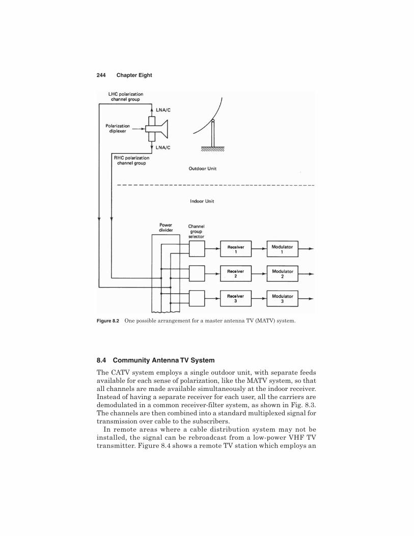
A master antenna TV (MATV) system is used to provide reception ofDBS TV/FM channels to a small group of users, for example, to thetenants in an apartment building. It consists of a single outdoor unit(antenna and LNA/C) feeding a number of indoor units, as shown inFig. 8.2. It is basically similar to the home system already described,but with each user having access to all the channels independentlyof the other users. The advantage is that only one outdoor unit isrequired, but as shown, separate LNA/Cs and feeder cables arerequired for each sense of polarization. Compared with the single-user system, a larger antenna is also required (2- to 3-m diameter)in order to maintain a good signal-to-noise ratio at all the indoorunits.
Where more than a few subscribers are involved, the distributionsystem used is similar to the community antenna (CATV) systemdescribed in the following section.
The Earth Segment 243
8.4 Community Antenna TV System
The CATV system employs a single outdoor unit, with separate feedsavailable for each sense of polarization, like the MATV system, so thatall channels are made available simultaneously at the indoor receiver.Instead of having a separate receiver for each user, all the carriers aredemodulated in a common receiver-filter system, as shown in Fig. 8.3.The channels are then combined into a standard multiplexed signal fortransmission over cable to the subscribers.
In remote areas where a cable distribution system may not beinstalled, the signal can be rebroadcast from a low-power VHF TVtransmitter. Figure 8.4 shows a remote TV station which employs an
244 Chapter Eight
Figure 8.2 One possible arrangement for a master antenna TV (MATV) system.

8-m (26.2-ft) antenna for reception of the satellite TV signal in theC band.
With the CATV system, local programming material also may be dis-tributed to subscribers, an option which is not permitted in the MATVsystem.
The Earth Segment 245
Figure 8.3 One possible arrangement for the indoor unit of a community antennaTV (CATV) system.
Figure 8.4 Remote television station. (Courtesy of TelesatCanada, 1983.)

8.5 Transmit-Receive Earth Stations
In the previous sections, receive-only TV stations are described.Obviously, somewhere a transmit station must complete the uplink tothe satellite. In some situations, a transmit-only station is required, forexample, in relaying TV signals to the remote TVRO stations alreadydescribed. Transmit-receive stations provide both functions and arerequired for telecommunications traffic generally, including network TV.The uplink facilities for digital TV are highly specialized and are coveredin Chap. 16.
The basic elements for a redundant earth station are shown in Fig. 8.5.As mentioned in connection with transponders in Sec. 7.7.1, redundancymeans that certain units are duplicated. A duplicate, or redundant,unit is automatically switched into a circuit to replace a correspon-ding unit that has failed. Redundant units are shown by dashed linesin Fig. 8.5.
The block diagram is shown in more detail in Fig. 8.6, where, for clar-ity, redundant units are not shown. Starting at the bottom of the diagram,the first block shows the interconnection equipment required betweensatellite station and the terrestrial network. For the purpose of explana-tion, telephone traffic will be assumed. This may consist of a number oftelephone channels in a multiplexed format. Multiplexing is a method ofgrouping telephone channels together, usually in basic groups of 12, with-out mutual interference. It is described in detail in Chaps. 9 and 10.
It may be that groupings different from those used in the terrestrialnetwork are required for satellite transmission, and the next block showsthe multiplexing equipment in which the reformatting is carried out.Following along the transmit chain, the multiplexed signal is modulatedonto a carrier wave at an intermediate frequency, usually 70 MHz.Parallel IF stages are required, one for each microwave carrier to betransmitted. After amplification at the 70-MHz IF, the modulated signalis then upconverted to the required microwave carrier frequency. Anumber of carriers may be transmitted simultaneously, and althoughthese are at different frequencies they are generally specified by theirnominal frequency, for example, as 6-GHz or 14-GHz carriers.
It should be noted that the individual carriers may be multidestina-tion carriers. This means that they carry traffic destined for differentstations. For example, as part of its load, a microwave carrier may havetelephone traffic for Boston and New York. The same carrier is receivedat both places, and the designated traffic sorted out by filters at thereceiving earth station.
Referring again to the block diagram of Fig. 8.6, after passing throughthe upconverters, the carriers are combined, and the resulting widebandsignal is amplified. The wideband power signal is fed to the antenna
246 Chapter Eight

247
Fig
ure
8.5
Bas
ic e
lem
ents
of
a re
dun
dan
t ea
rth
sta
tion
. (C
ourt
esy
of T
eles
at C
anad
a, 1
983.
)

through a diplexer, which allows the antenna to handle transmit andreceive signals simultaneously.
The station’s antenna functions in both, the transmit and receivemodes, but at different frequencies. In the C band, the nominal uplink,or transmit, frequency is 6 GHz and the downlink, or receive, frequencyis nominally 4 GHz. In the Ku band, the uplink frequency is nominally14 GHz, and the downlink, 12 GHz. High-gain antennas are employedin both bands, which also means narrow antenna beams. A narrow beamis necessary to prevent interference between neighboring satellite links.In the case of C band, interference to and from terrestrial microwave
248 Chapter Eight
Figure 8.6 More detailed block diagram of a transmit-receive earth station.

links also must be avoided. Terrestrial microwave links do not operateat Ku-band frequencies.
In the receive branch (the right-hand side of Fig. 8.6), the incomingwideband signal is amplified in an LNA and passed to a divider network,which separates out the individual microwave carriers. These are eachdownconverted to an IF band and passed on to the multiplex block,where the multiplexed signals are reformatted as required by the ter-restrial network.
It should be noted that, in general, the signal traffic flow on the receiveside will differ from that on the transmit side. The incoming microwavecarriers will be different in number and in the amount of traffic carried,and the multiplexed output will carry telephone circuits not necessar-ily carried on the transmit side.
A number of different classes of earth stations are available, depend-ing on the service requirements. Traffic can be broadly classified asheavy route, medium route, and thin route. In a thin-route circuit, atransponder channel (36 MHz) may be occupied by a number of singlecarriers, each associated with its own voice circuit. This mode of oper-ation is known as single carrier per channel (SCPC), a multiple-accessmode which is discussed further in Chap. 14. Antenna sizes range from3.6 m (11.8 ft) for transportable stations up to 30 m (98.4 ft) for a mainterminal.
A medium-route circuit also provides multiple access, either on thebasis of frequency-division multiple access (FDMA) or time-division mul-tiple access (TDMA), multiplexed baseband signals being carried ineither case. These access modes are also described in detail in Chap. 14.Antenna sizes range from 30 m (89.4 ft) for a main station to 10 m (32.8 ft)for a remote station.
In a 6/4-GHz heavy-route system, each satellite channel (bandwidth36 MHz) is capable of carrying over 960 one-way voice circuits simulta-neously or a single-color analog TV signal with associated audio (in somesystems two analog TV signals can be accommodated). Thus the transpon-der channel for a heavy-route circuit carries one large-bandwidth signal,which may be TV or multiplexed telephony. The antenna diameter for aheavy-route circuit is at least 30 m (98.4 ft). For international operationsuch antennas are designed to the INTELSAT specifications for aStandard A earth station (Intelsat, 1982). Figure 8.7 shows a photographof a 32-m (105-ft) Standard A earth station antenna.
It will be appreciated that for these large antennas, which may weighin the order of 250 tons, the foundations must be very strong and stable.Such large diameters automatically mean very narrow beams, andtherefore, any movement which would deflect the beam unduly must beavoided. Where snow and ice conditions are likely to be encountered,built-in heaters are required. For the antenna shown in Fig. 8.7, deicing
The Earth Segment 249

heaters provide reflector surface heat of 40W/ft2 for the main reflectorsand subreflectors, and 3000 W for the azimuth wheels.
Although these antennas are used with geostationary satellites, somedrift in the satellite position does occur, as shown in Chap. 3. This, com-bined with the very narrow beams of the larger earth station antennas,means that some provision must be made for a limited degree of track-ing. Step adjustments in azimuth and elevation may be made, undercomputer control, to maximize the received signal.
The continuity of the primary power supply is another important con-sideration in the design of transmit-receive earth stations. Apart from thesmallest stations, power backup in the form of multiple feeds from thecommercial power source and/or batteries and generators is provided. Ifthe commercial power fails, batteries immediately take over with no inter-ruption. At the same time, the standby generators start up, and oncethey are up to speed they automatically take over from the batteries.
8.6 Problems and Exercises
8.1. Explain what is meant by DBS service. How does this differ from thehome reception of satellite TV signals in the C band?
250 Chapter Eight
Figure 8.7 Standard-A (C-band 6/4 GHz) 32-m antenna.(Courtesy of TIW Systems, Inc., Sunnydale, CA.)

8.2. Explain what is meant by polarization interleaving. On a frequency axis,draw to scale the channel allocations for the 32 TV channels in the Ku band,showing how polarization interleaving is used in this.
8.3. Why is it desirable to downconvert the satellite TV signal received at theantenna?
8.4. Explain why the LNA in a satellite receiving system is placed at theantenna end of the feeder cable.
8.5. With the aid of a block schematic, briefly describe the functioning of theindoor receiving unit of a satellite TV/FM receiving system intended for homereception.
8.6. In most satellite TV receivers the first IF band is converted to a second,fixed IF. Why is this second frequency conversion required?
8.7. For the standard home television set to function in a satellite TV/FMreceiving system, a demodulator/remodulator unit is needed. Explain why.
8.8. Describe and compare the MATV and the CATV systems.
8.9. Explain what is meant by the term redundant earth station.
8.10. With the aid of a block schematic, describe the functioning of a transmit-receive earth station used for telephone traffic. Describe a multidestinationcarrier.
References
Huck, R. W., and J. W. B. Day. 1979. “Experience in Satellite Broadcasting Applicationswith CTS/HERMES.” XIth International TV Symposium, Montreux, 27 May–1 June.
INTELSAT. 1982. “Standard A Performance Characteristics of Earth Stations in theINTELSAT IV, IVA, and V Systems.” BG-28-72E M/6/77.
Orbit, 2005, at http://orbitmagazine.com/Satellite Theater systems, 2005, at http://www.satellitetheater.com/
The Earth Segment 251

351
Chapter
12The Space Link
12.1 Introduction
This chapter describes how the link-power budget calculations are made.These calculations basically relate two quantities, the transmit powerand the receive power, and show in detail how the difference betweenthese two powers is accounted for.
Link-budget calculations are usually made using decibel or decilogquantities. These are explained in App. G. In this text [square] brack-ets are used to denote decibel quantities using the basic power defini-tion. Where no ambiguity arises regarding the units, the abbreviationdB is used. For example, Boltzmann’s constant is given as 228.6 dB,although, strictly speaking, this should be given as 228.6 decilogs rel-ative to 1 J/K. Where it is desirable to show the reference unit, this isindicated in the abbreviation, for example, dBHz means decibels rela-tive to 1 Hz.
12.2 Equivalent Isotropic Radiated Power
A key parameter in link-budget calculations is the equivalent isotropicradiated power, conventionally denoted as EIRP. From Eqs. (6.4) and(6.5), the maximum power flux density at some distance r from a trans-mitting antenna of gain G is
(12.1)
An isotropic radiator with an input power equal to GPS would producethe same flux density. Hence, this product is referred to as the EIRP, or
(12.2)EIRP GPS
M GPS
4r2

352 Chapter Twelve
EIRP is often expressed in decibels relative to 1 W, or dBW. Let PS bein watts; then
(12.3)
where [PS] is also in dBW and [G] is in dB.
Example 12.1 A satellite downlink at 12 GHz operates with a transmit power of6 W and an antenna gain of 48.2 dB. Calculate the EIRP in dBW.
Solution
56 dBW
For a paraboloidal antenna, the isotropic power gain is given by Eq.(6.32). This equation may be rewritten in terms of frequency, since thisis the quantity which is usually known.
(12.4)
where f is the carrier frequency in GHz, D is the reflector diameter inm, and is the aperture efficiency. A typical value for aperture effi-ciency is 0.55, although values as high as 0.73 have been specified(Andrew Antenna, 1985).
With the diameter D in feet and all other quantities as before, theequation for power gain becomes
(12.5)
Example 12.2 Calculate the gain in decibels of a 3-m paraboloidal antenna oper-ating at a frequency of 12 GHz. Assume an aperture efficiency of 0.55.
Solution
Hence,
[G] 10 log 78168 48.9 dB
12.3 Transmission Losses
The [EIRP] may be thought of as the power input to one end of thetransmission link, and the problem is to find the power received at theother end. Losses will occur along the way, some of which are constant.
G 0.55 (10.472 12 3)2 > 78168
G (3.192fD)2
G (10.472fD)2
[EIRP] 10 loga6W1Wb 48.2
[EIRP] [PS] [G] dBW

Other losses can only be estimated from statistical data, and some ofthese are dependent on weather conditions, especially on rainfall.
The first step in the calculations is to determine the losses for clear-weather or clear-sky conditions. These calculations take into account thelosses, including those calculated on a statistical basis, which do not varysignificantly with time. Losses which are weather-related, and otherlosses which fluctuate with time, are then allowed for by introducingappropriate fade margins into the transmission equation.
12.3.1 Free-space transmission
As a first step in the loss calculations, the power loss resulting from thespreading of the signal in space must be determined. This calculation is sim-ilar for the uplink and the downlink of a satellite circuit. Using Eqs. (12.1)and (12.2) gives the power-flux density at the receiving antenna as
(12.6)
The power delivered to a matched receiver is this power-flux densitymultiplied by the effective aperture of the receiving antenna, given byEq. (6.15). The received power is therefore
(12.7)
Recall that r is the distance, or range, between the transmit andreceive antennas and GR is the isotropic power gain of the receivingantenna. The subscript R is used to identify the receiving antenna.
The right-hand side of Eq. (12.7) is separated into three terms asso-ciated with the transmitter, receiver, and free space, respectively. Indecibel notation, the equation becomes
(12.8)
The received power in dBW is therefore given as the sum of the trans-mitted EIRP in dBW plus the receiver antenna gain in dB minus a thirdterm, which represents the free-space loss in decibels. The free-space losscomponent in decibels is given by
(12.9)[FSL] 10 loga4rl b
2
[PR] [EIRP] [GR] 10 loga4rl b
2
PR MAeff
EIRP
4r2 l2GR
4
(EIRP)(GR)a l4rb2
M EIRP
4r2
The Space Link 353
Normally, the frequency rather than wavelength will be known, andthe substitution l c/f can be made, where c 108 m/s. With frequencyin megahertz and distance in kilometers, it is left as an exercise for thestudent to show that the free-space loss is given by
(12.10)
Equation (12.8) can then be written as
(12.11)
The received power [PR] will be in dBW when the [EIRP] is in dBW, and[FSL] in dB. Equation (12.9) is applicable to both the uplink and thedownlink of a satellite circuit, as will be shown in more detail shortly.
Example 12.3 The range between a ground station and a satellite is 42,000 km.Calculate the free-space loss at a frequency of 6 GHz.
Solution
[FSL] 32.4 20 log 42,000 20 log 6000 200.4 dB
This is a very large loss. Suppose that the [EIRP] is 56 dBW (as calcu-lated in Example 12.1 for a radiated power of 6 W) and the receive antennagain is 50 dB. The receive power would be 56 50 200.4 94.4 dBW.This is 355 pW. It also may be expressed as 64.4 dBm, which is 64.4 dBbelow the 1-mW reference level.
Equation (12.11) shows that the received power is increased byincreasing antenna gain as expected, and Eq. (6.32) shows that antennagain is inversely proportional to the square of the wavelength. Hence,it might be thought that increasing the frequency of operation (andtherefore decreasing wavelength) would increase the received power.However, Eq. (12.9) shows that the free-space loss is also inversely pro-portional to the square of the wavelength, so these two effects cancel.It follows, therefore, that for a constant EIRP, the received power isindependent of frequency of operation.
If the transmit power is a specified constant, rather than the EIRP,then the received power will increase with increasing frequency forgiven antenna dish sizes at the transmitter and receiver. It is left as anexercise for the student to show that under these conditions the receivedpower is directly proportional to the square of the frequency.
12.3.2 Feeder losses
Losses will occur in the connection between the receive antenna and thereceiver proper. Such losses will occur in the connecting waveguides,filters, and couplers. These will be denoted by RFL, or [RFL] dB, for receiver
[PR] [EIRP] [GR] [FSL]
[FSL] 32.4 20 log r 20 log f
354 Chapter Twelve
feeder losses. The [RFL] values are added to [FSL] in Eq. (12.11). Similarlosses will occur in the filters, couplers, and waveguides connectingthe transmit antenna to the high-power amplifier (HPA) output.However, provided that the EIRP is stated, Eq. (12.11) can be usedwithout knowing the transmitter feeder losses. These are needed onlywhen it is desired to relate EIRP to the HPA output, as described inSecs. 12.7.4 and 12.8.2.
12.3.3 Antenna misalignment losses
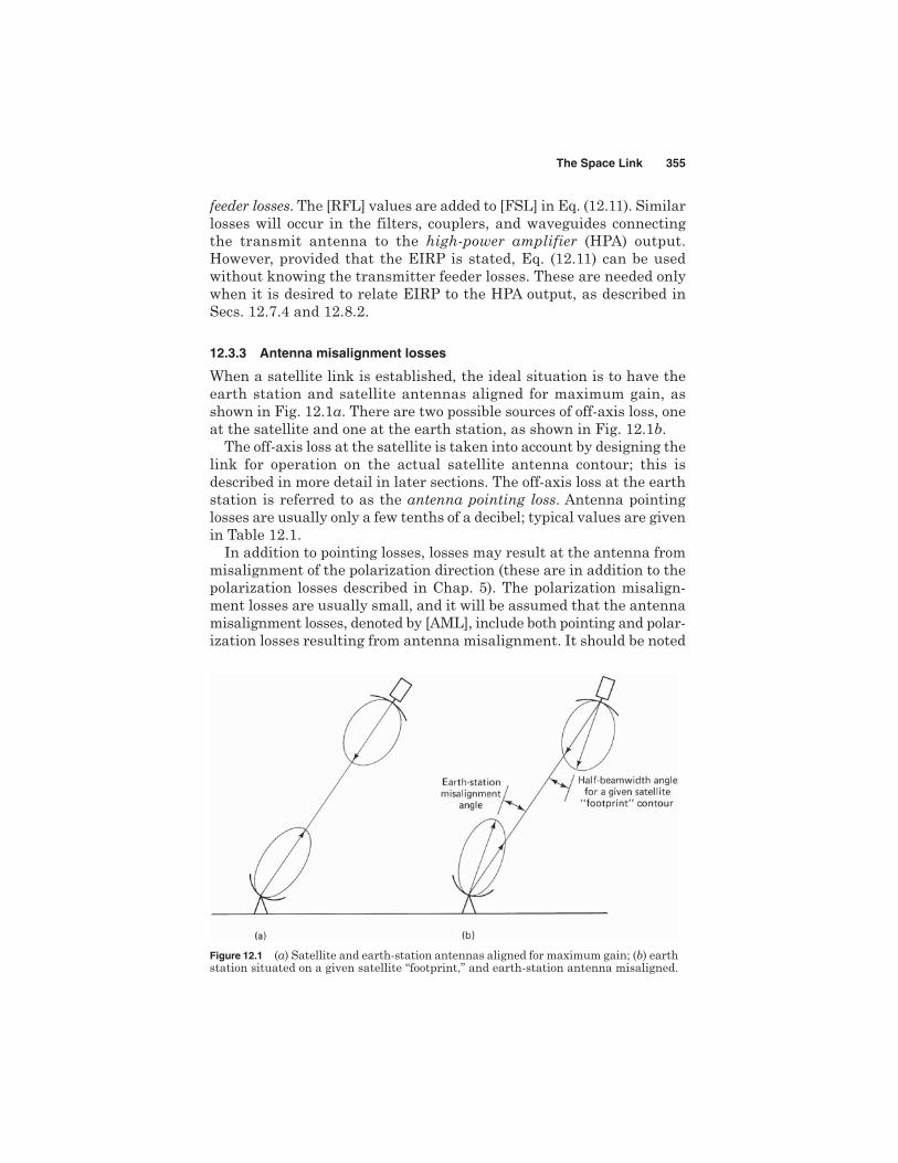
When a satellite link is established, the ideal situation is to have theearth station and satellite antennas aligned for maximum gain, asshown in Fig. 12.1a. There are two possible sources of off-axis loss, oneat the satellite and one at the earth station, as shown in Fig. 12.1b.
The off-axis loss at the satellite is taken into account by designing thelink for operation on the actual satellite antenna contour; this isdescribed in more detail in later sections. The off-axis loss at the earthstation is referred to as the antenna pointing loss. Antenna pointinglosses are usually only a few tenths of a decibel; typical values are givenin Table 12.1.
In addition to pointing losses, losses may result at the antenna frommisalignment of the polarization direction (these are in addition to thepolarization losses described in Chap. 5). The polarization misalign-ment losses are usually small, and it will be assumed that the antennamisalignment losses, denoted by [AML], include both pointing and polar-ization losses resulting from antenna misalignment. It should be noted
The Space Link 355
Figure 12.1 (a) Satellite and earth-station antennas aligned for maximum gain; (b) earthstation situated on a given satellite “footprint,” and earth-station antenna misaligned.

that the antenna misalignment losses have to be estimated from sta-tistical data, based on the errors actually observed for a large numberof earth stations, and of course, the separate antenna misalignmentlosses for the uplink and the downlink must be taken into account.
12.3.4 Fixed atmosphericand ionospheric losses
Atmospheric gases result in losses by absorption, as described in Sec.4.2 and by Eq. (4.1). These losses usually amount to a fraction of a deci-bel, and in subsequent calculations, the decibel value will be denoted by[AA]. Values obtained for some locations in the Province of Ontario,Canada, are shown in Table 12.1. Also, as discussed in Sec. 5.5, the ion-osphere introduces a depolarization loss given by Eq. (5.19), and in sub-sequent calculations, the decibel value for this will be denoted by [PL].
12.4 The Link-Power Budget Equation
As mentioned at the beginning of Sec. 12.3, the [EIRP] can be consid-ered as the input power to a transmission link. Now that the losses forthe link have been identified, the power at the receiver, which is thepower output of the link, may be calculated simply as [EIRP] [LOSSES] [GR], where the last quantity is the receiver antenna gain.Note carefully that decibel addition must be used.
356 Chapter Twelve
TABLE 12.1 Atmospheric Absorption Loss and Satellite Pointing Loss for Cities andCommunities in the Province of Ontario
Atmospheric absorptionSatellite antenna pointing loss, dB
Location dB, summer 1/4 Canada coverage 1/2 Canada coverage
Cat Lake 0.2 0.5 0.5Fort Severn 0.2 0.9 0.9Geraldton 0.2 0.2 0.1Kingston 0.2 0.5 0.4London 0.2 0.3 0.6North Bay 0.2 0.3 0.2Ogoki 0.2 0.4 0.3Ottawa 0.2 0.6 0.2Sault Ste. Marie 0.2 0.1 0.3Sioux Lookout 0.2 0.4 0.3Sudbury 0.2 0.3 0.2Thunder Bay 0.2 0.3 0.2Timmins 0.2 0.5 0.2Toronto 0.2 0.3 0.4Windsor 0.2 0.5 0.8
SOURCE: Telesat Canada Design Workbook.

The major source of loss in any ground-satellite link is the free-spacespreading loss [FSL], as shown in Sec. 12.3.1, where Eq. (12.13) is thebasic link-power budget equation taking into account this loss only.However, the other losses also must be taken into account, and these aresimply added to [FSL]. The losses for clear-sky conditions are
[LOSSES] [FSL] [RFL] [AML] [AA] [PL] (12.12)
The decibel equation for the received power is then
[PR] [EIRP] [GR] [LOSSES] (12.13)
where [PR] received power, dBW[EIRP] equivalent isotropic radiated power, dBW[FSL] free-space spreading loss, dB[RFL] receiver feeder loss, dB
[AML] antenna misalignment loss, dB[AA] atmospheric absorption loss, dB[PL] polarization mismatch loss, dB
Example 12.4 A satellite link operating at 14 GHz has receiver feeder losses of1.5 dB and a free-space loss of 207 dB. The atmospheric absorption loss is 0.5 dB,and the antenna pointing loss is 0.5 dB. Depolarization losses may be neglected.Calculate the total link loss for clear-sky conditions.
Solution The total link loss is the sum of all the losses:
[LOSSES] [FSL] [RFL] [AA] [AML]
207 1.5 0.5 0.5
209.5 dB
12.5 System Noise
It is shown in Sec. 12.3 that the receiver power in a satellite link is verysmall, on the order of picowatts. This by itself would be no problembecause amplification could be used to bring the signal strength up toan acceptable level. However, electrical noise is always present at theinput, and unless the signal is significantly greater than the noise,amplification will be of no help because it will amplify signal and noiseto the same extent. In fact, the situation will be worsened by the noiseadded by the amplifier.
The major source of electrical noise in equipment is that which arisesfrom the random thermal motion of electrons in various resistive andactive devices in the receiver. Thermal noise is also generated in the
The Space Link 357

lossy components of antennas, and thermal-like noise is picked up bythe antennas as radiation.
The available noise power from a thermal noise source is given by
(12.14)
Here, TN is known as the equivalent noise temperature, BN is the equiv-alent noise bandwidth, and k 1.38 1023 J/K is Boltzmann’s con-stant. With the temperature in kelvins and bandwidth in hertz, thenoise power will be in watts. The noise power bandwidth is alwayswider than the 3-dB bandwidth determined from the amplitude-fre-quency response curve, and a useful rule of thumb is that the noisebandwidth is equal to 1.12 times the 3-dB bandwidth, or BN ≈ 1.12 B3dB. The bandwidths here are in hertz (or a multiple such as MHz).
The main characteristic of thermal noise is that it has a flat frequencyspectrum; that is, the noise power per unit bandwidth is a constant. Thenoise power per unit bandwidth is termed the noise power spectral den-sity. Denoting this by N0, then from Eq. (12.14),
(12.15)
The noise temperature is directly related to the physical temperatureof the noise source but is not always equal to it. This is discussed morefully in the following sections. The noise temperatures of various sourceswhich are connected together can be added directly to give the total noise.
Example 12.5 An antenna has a noise temperature of 35 K and is matched intoa receiver which has a noise temperature of 100 K. Calculate (a) the noise powerdensity and (b) the noise power for a bandwidth of 36 MHz.
Solution
(a) N0 (35 100) 1.38 1023 1.86 1021 J
(b) PN 1.86 1021 36 106
0.067 pW
In addition to these thermal noise sources, intermodulation distortionin high-power amplifiers (see Sec. 12.7.3) can result in signal productswhich appear as noise and in fact is referred to as intermodulationnoise. This is discussed in Sec. 12.10.
12.5.1 Antenna noise
Antennas operating in the receiving mode introduce noise into the satel-lite circuit. Noise therefore will be introduced by the satellite receiveantenna and the ground station receive antenna. Although the physical
N0 5PN
BN5 kTN J
PN kTNBN
358 Chapter Twelve

origins of the noise in either case are similar, the magnitudes of theeffects differ significantly.
The antenna noise can be broadly classified into two groups: noise orig-inating from antenna losses and sky noise. Sky noise is a term used todescribe the microwave radiation which is present throughout the uni-verse and which appears to originate from matter in any form at finitetemperatures. Such radiation in fact covers a wider spectrum than justthe microwave spectrum. The equivalent noise temperature of the sky, asseen by an earth-station antenna, is shown in Fig. 12.2. The lower graphis for the antenna pointing directly overhead, while the upper graph isfor the antenna pointing just above the horizon. The increased noise inthe latter case results from the thermal radiation of the earth, and thisin fact sets a lower limit of about 5° at C band and 10° at Ku band on theelevation angle which may be used with ground-based antennas.
The graphs show that at the low-frequency end of the spectrum, thenoise decreases with increasing frequency. Where the antenna is zenith-pointing, the noise temperature falls to about 3 K at frequencies between
The Space Link 359
Figure 12.2 Irreducible noise temperature of an ideal, ground-based antenna. Theantenna is assumed to have a very narrow beam without sidelobes or electricallosses. Below 1 GHz, the maximum values are for the beam pointed at the galacticpoles. At higher frequencies, the maximum values are for the beam just above thehorizon and the minimum values for zenith pointing. The low-noise region between1 and 10 GHz is most amenable to application of special, low-noise antennas. (FromPhilip F. Panter, “Communications Systems Design,” McGraw-Hill Book Company,New York, 1972. With permission.)

about 1 and 10 GHz. This represents the residual background radiationin the universe. Above about 10 GHz, two peaks in temperature areobserved, resulting from resonant losses in the earth’s atmosphere.These are seen to coincide with the peaks in atmospheric absorption lossshown in Fig. 4.2.
Any absorptive loss mechanism generates thermal noise, there being adirect connection between the loss and the effective noise temperature, asshown in Sec. 12.5.5. Rainfall introduces attenuation, and therefore, itdegrades transmissions in two ways: It attenuates the signal, and it intro-duces noise. The detrimental effects of rain are much worse at Ku-bandfrequencies than at C band, and the downlink rain-fade margin, discussedin Sec. 12.9.2, must also allow for the increased noise generated.
Figure 12.2 applies to ground-based antennas. Satellite antennas aregenerally pointed toward the earth, and therefore, they receive the fullthermal radiation from it. In this case the equivalent noise temperatureof the antenna, excluding antenna losses, is approximately 290 K.
Antenna losses add to the noise received as radiation, and the totalantenna noise temperature is the sum of the equivalent noise tempera-tures of all these sources. For large ground-based C-band antennas, thetotal antenna noise temperature is typically about 60 K, and for the Kuband, about 80 K under clear-sky conditions. These values do not applyto any specific situation and are quoted merely to give some idea of themagnitudes involved. Figure 12.3 shows the noise temperature as a func-tion of angle of elevation for a 1.8-m antenna operating in the Ku band.
12.5.2 Amplifier noise temperature
Consider first the noise representation of the antenna and the low noiseamplifier (LNA) shown in Fig. 12.4a. The available power gain of theamplifier is denoted as G, and the noise power output, as Pno. For the
360 Chapter Twelve
Figure 12.3 Antenna noise temperature as a function of elevation for 1.8-m antenna char-acteristics. (Andrew Bulletin 1206; courtesy of Andrew Antenna Company, Limited.)

moment we will work with the noise power per unit bandwidth, whichis simply noise energy in joules as shown by Eq. (12.15). The input noiseenergy coming from the antenna is
N0,ant kTant (12.16)
The output noise energy N0,out will be GN0,ant plus the contributionmade by the amplifier. Now all the amplifier noise, wherever it occursin the amplifier, may be referred to the input in terms of an equivalentinput noise temperature for the amplifier Te. This allows the outputnoise to be written as
N0,out Gk(Tant Te) (12.17)
The total noise referred to the input is simply N0,out /G, or
N0,in k(Tant Te) (12.18)
Te can be obtained by measurement, a typical value being in the range35 to 100 K. Typical values for Tant are given in Sec. 12.5.1.
12.5.3 Amplifiers in cascade
The cascade connection is shown in Fig. 12.4b. For this arrangement,the overall gain is
G G1G2 (12.19)
The Space Link 361
Figure 12.4 Circuit used in finding equivalent noise tempera-ture of (a) an amplifier and (b) two amplifiers in cascade.

The noise energy of amplifier 2 referred to its own input is simply kTe2.The noise input to amplifier 2 from the preceding stages is G1k(Tant Te1), and thus the total noise energy referred to amplifier 2 input is
N0,2 G1k(Tant Te1) kTe2 (12.20)
This noise energy may be referred to amplifier 1 input by dividing bythe available power gain of amplifier 1:
(12.21)
A system noise temperature may now be defined as TS by
N0,1 kTS (12.22)
and hence it will be seen that TS is given by
(12.23)
This is a very important result. It shows that the noise temperatureof the second stage is divided by the power gain of the first stage whenreferred to the input. Therefore, in order to keep the overall systemnoise as low as possible, the first stage (usually an LNA) should havehigh power gain as well as low noise temperature.
This result may be generalized to any number of stages in cascade,giving
(12.24)
12.5.4 Noise factor
An alternative way of representing amplifier noise is by means of itsnoise factor, F. In defining the noise factor of an amplifier, the source istaken to be at room temperature, denoted by T0, usually taken as 290 K.The input noise from such a source is kT0, and the output noise from theamplifier is
N0,out FGkT0 (12.25)
Here, G is the available power gain of the amplifier as before, and F isits noise factor.
TS Tant Te1 Te2
G1
Te3
G1G2
c
TS Tant Te1 Te2
G1
N0,1 N0,2
G1
kaTant Te1 Te2
G1
b
362 Chapter Twelve
A simple relationship between noise temperature and noise factorcan be derived. Let Te be the noise temperature of the amplifier, and letthe source be at room temperature as required by the definition of F.This means that Tant T0. Since the same noise output must be avail-able whatever the representation, it follows that
Gk(T0 Te) FGkT0
or
Te (F 1) T0 (12.26)
This shows the direct equivalence between noise factor and noise tem-perature. As a matter of convenience, in a practical satellite receivingsystem, noise temperature is specified for low-noise amplifiers and con-verters, while noise factor is specified for the main receiver unit.
The noise figure is simply F expressed in decibels:
Noise figure [F] 10 log F (12.27)
Example 12.6 An LNA is connected to a receiver which has a noise figure of 12dB. The gain of the LNA is 40 dB, and its noise temperature is 120 K. Calculatethe overall noise temperature referred to the LNA input.
Solution 12 dB is a power ratio of 15.85:1, and therefore,
Te2 (15.85 1) 290 4306 K
A gain of 40 dB is a power ratio of 104:1, and therefore,
120.43 K
In Example 12.6 it will be seen that the decibel quantities must be con-verted to power ratios. Also, even though the main receiver has a veryhigh noise temperature, its effect is made negligible by the high gain ofthe LNA.
12.5.5 Noise temperatureof absorptive networks
An absorptive network is one which contains resistive elements. Theseintroduce losses by absorbing energy from the signal and converting itto heat. Resistive attenuators, transmission lines, and waveguides areall examples of absorptive networks, and even rainfall, which absorbsenergy from radio signals passing through it, can be considered a form
Tin 120 4306
104
The Space Link 363

of absorptive network. Because an absorptive network contains resist-ance, it generates thermal noise.
Consider an absorptive network, which has a power loss L. The powerloss is simply the ratio of input power to output power and will alwaysbe greater than unity. Let the network be matched at both ends, to a ter-minating resistor, RT, at one end and an antenna at the other, as shownin Fig. 12.5, and let the system be at some ambient temperature Tx. Thenoise energy transferred from RT into the network is kTx. Let the net-work noise be represented at the output terminals (the terminals con-nected to the antenna in this instance) by an equivalent noisetemperature TNW,0. Then the noise energy radiated by the antenna is
(12.28)
Because the antenna is matched to a resistive source at temperatureTx, the available noise energy which is fed into the antenna and radi-ated is Nrad kTx. Keep in mind that the antenna resistance to whichthe network is matched is fictitious, in the sense that it represents radi-ated power, but it does not generate noise power. This expression for Nrad
can be substituted into Eq. (12.28) to give
(12.29)
This is the equivalent noise temperature of the network referred tothe output terminals of the network. The equivalent noise at the outputcan be transferred to the input on dividing by the network power gain,which by definition is 1/L. Thus, the equivalent noise temperature of thenetwork referred to the network input is
TNW,i Tx(L 1) (12.30)
Since the network is bilateral, Eqs. (12.29) and (12.30) apply for signalflow in either direction. Thus, Eq. (12.30) gives the equivalent noise
TNW,0 Txa1 1Lb
Nrad kTx
L kTNW,0
364 Chapter Twelve
RT
Lossy networkpower loss L : 1
Ambient temperatureTX
NRAD
Figure 12.5 Network matched at both ends, to a terminating resistor RT atone end and an antenna at the other.

temperature of a lossy network referred to the input at the antennawhen the antenna is used in receiving mode.
If the lossy network should happen to be at room temperature, thatis, Tx T0, then a comparison of Eqs. (12.26) and (12.30) shows that
F L (12.31)
This shows that at room temperature the noise factor of a lossy networkis equal to its power loss.
12.5.6 Overall system noise temperature
Figure 12.6a shows a typical receiving system. Applying the results ofthe previous sections yields, for the system noise temperature referredto the input,
(12.32)
The significance of the individual terms is illustrated in the followingexamples.
Example 12.7 For the system shown in Fig. 12.6a, the receiver noise figure is12 dB, the cable loss is 5 dB, the LNA gain is 50 dB, and its noise temperature150 K. The antenna noise temperature is 35 K. Calculate the noise temperaturereferred to the input.
Solution For the main receiver, F 101.2 15.85. For the cable, L 100.5
3.16.For the LNA, G 105. Hence,
185 K>
TS 35 150 (3.16 1) 290
105
3.16 (15.85 1) 290
105
TS Tant Te1 (L 1)T0
G1
L(F 1)T0
G1
The Space Link 365
Figure 12.6 Connections used in examples illustrating overall noisetemperature of system, Sec. 12.5.6.

Example 12.8 Repeat the calculation when the system of Fig. 12.6a is arrangedas shown in Fig. 12.6b.
Solution In this case the cable precedes the LNA, and therefore, the equivalentnoise temperature referred to the cable input is
1136 K
Examples 12.7 and 12.8 illustrate the important point that the LNAmust be placed ahead of the cable, which is why one sees amplifiersmounted right at the dish in satellite receive systems.
12.6 Carrier-to-Noise Ratio
Ameasure of the performance of a satellite link is the ratio of carrier powerto noise power at the receiver input, and link-budget calculations are oftenconcerned with determining this ratio. Conventionally, the ratio is denotedby C/N (or CNR), which is equivalent to PR/PN. In terms of decibels,
(12.33)
Equations (12.17) and (12.18) may be used for [PR] and [PN], resulting in
(12.34)
The G/T ratio is a key parameter in specifying the receiving systemperformance. The antenna gain GR and the system noise temperatureTS can be combined in Eq. (12.34) as
[G/T] [GR] [TS] dBK1 (12.35)
Therefore, the link equation [Eq. (12.34)] becomes
(12.36)
The ratio of carrier power to noise power density PR/N0 may be thequantity actually required. Since PN kTNBN N0BN, then
c CN0
d [BN]
cCNd c C
N0BN
d
cCNd [EIRP] cG
Td [LOSSES] [k] [BN]
cCNd [EIRP] [GR] [LOSSES] [k] [TS] [BN]
cCNd [PR] [PN]
TS 35 (3.16 1) 290 3.16 150 3.16 (15.85 1) 290
105
366 Chapter Twelve
and therefore
(12.37)
[C/N] is a true power ratio in units of decibels, and [BN] is in decibelsrelative to 1 Hz, or dBHz. Thus, the units for [C/N0] are dBHz.
Substituting Eq. (12.37) for [C/N] gives
(12.38)
Example 12.9 In a link-budget calculation at 12 GHz, the free-space loss is 206dB, the antenna pointing loss is 1 dB, and the atmospheric absorption is 2 dB. Thereceiver [G/T] is 19.5 dB/K, and receiver feeder losses are 1 dB. The EIRP is 48dBW. Calculate the carrier-to-noise spectral density ratio.
Solution The data are best presented in tabular form and in fact lend themselvesreadily to spreadsheet-type computations. For brevity, the units are shown asdecilogs, (see App. G) and losses are entered as negative numbers to take accountof the minus sign in Eq. (12.38). Recall that Boltzmann’s constant equates to228.6 decilogs, so [k] 228.6 decilogs, as shown in the following table.
Entering data in this way allows the final result to be entered in atable cell as the sum of the terms in the rows above the cell, a featureusually incorporated in spreadsheets and word processors. This is illus-trated in the following table.
The final result, 86.10 dBHz, is the algebraic sum of the quantitiesas given in Eq. (12.38).
12.7 The Uplink
The uplink of a satellite circuit is the one in which the earth station istransmitting the signal and the satellite is receiving it. Equation (12.38)can be applied to the uplink, but subscript U will be used to denote
Quantity Decilogs
Free-space loss 206Atmospheric absorption loss 2Antenna pointing loss 1Receiver feeder losses 1Polarization mismatch loss 0Receiver G/T ratio 19.5EIRP 48[k] 228.6[C/N0], Eq. (12.38) 86.1
c CN0
d [EIRP] cGTd [LOSSES] [k]
c CN0
d cCNd [BN]
The Space Link 367

specifically that the uplink is being considered. Thus Eq. (12.38)becomes
(12.39)
In Eq. (12.39) the values to be used are the earth station EIRP, thesatellite receiver feeder losses, and satellite receiver G/T. The free-spaceloss and other losses which are frequency-dependent are calculated forthe uplink frequency. The resulting carrier-to-noise density ratio givenby Eq. (12.39) is that which appears at the satellite receiver.
In some situations, the flux density appearing at the satellite receiveantenna is specified rather than the earth-station EIRP, and Eq. (12.39)is modified as explained next.
12.7.1 Saturation flux density
As explained in Sec. 7.7.3, the traveling-wave tube amplifier (TWTA) ina satellite transponder exhibits power output saturation, as shown inFig. 7.21. The flux density required at the receiving antenna to producesaturation of the TWTA is termed the saturation flux density. The sat-uration flux density is a specified quantity in link budget calculations,and knowing it, one can calculate the required EIRP at the earth sta-tion. To show this, consider again Eq. (12.6) which gives the flux den-sity in terms of EIRP, repeated here for convenience:
In decibel notation this is
(12.40)
But from Eq. (12.9) for free-space loss we have
(12.41)
Substituting this in Eq. (12.40) gives
(12.42)
The l2/4 term has dimensions of area, and in fact, from Eq. (6.15) itis the effective area of an isotropic antenna. Denoting this by A0 gives
(12.43)[A0] 10 log l2
4
[M] [EIRP] [FSL] 10 log l2
4
[FSL] 10 log l2
4 10 log
14r2
[M] [EIRP] 10 log 1
4r2
M EIRP
4r2
c CN0
dU
[EIRP]U cGTd
U [LOSSES]U [k]
368 Chapter Twelve

Since frequency rather than wavelength is normally known, it is leftas an exercise for the student to show that with frequency f in gigahertz,Eq. (12.43) can be rewritten as
(12.44)
Combining this with Eq. (12.42) and rearranging slightly gives theEIRP as
(12.45)
Equation (12.45) was derived on the basis that the only loss presentwas the spreading loss, denoted by [FSL]. But, as shown in the pre-vious sections, the other propagation losses are the atmosphericabsorption loss, the polarization mismatch loss, and the antennamisalignment loss. When allowance is made for these, Eq. (12.45)becomes
(12.46)
In terms of the total losses given by Eq. (12.12), Eq. (12.46) becomes
(12.47)
This is for clear-sky conditions and gives the minimum value of [EIRP]which the earth station must provide to produce a given flux densityat the satellite. Normally, the saturation flux density will be specified.With saturation values denoted by the subscript S, Eq. (12.47) isrewritten as
(12.48)
Example 12.10 An uplink operates at 14 GHz, and the flux density required to sat-urate the transponder is 120 dB(W/m2). The free-space loss is 207 dB, and the otherpropagation losses amount to 2 dB. Calculate the earth-station [EIRP] required forsaturation, assuming clear-sky conditions. Assume [RFL] is negligible.
Solution At 14 GHz,
[A0] (21.45 20 log 14) 44.37 dB
The losses in the propagation path amount to 207 2 209 dB. Hence,from Eq. (12.48),
[EIRPS]U 120 44.37 209
44.63 dBW
[EIRPS]U [S] [A0] [LOSSES]U [RFL]
[EIRP] [M] [A0] [LOSSES] [RFL]
[EIRP] [M] [A0] [FSL] [AA] [PL] [AML]
[EIRP] [M] [A0] [FSL]
[A0] (21.45 20 log f)
The Space Link 369
12.7.2 Input backoff
As described in Sec. 12.7.3, where a number of carriers are present simul-taneously in a TWTA, the operating point must be backed off to a linearportion of the transfer characteristic to reduce the effects of intermodu-lation distortion. Such multiple carrier operation occurs with frequency-division multiple access (FDMA), which is described in Chap. 14. Thepoint to be made here is that backoff (BO) must be allowed for in the link-budget calculations.
Suppose that the saturation flux density for single-carrier operation isknown. Input BO will be specified for multiple-carrier operation, referredto the single-carrier saturation level. The earth-station EIRP will haveto be reduced by the specified BO, resulting in an uplink value of
[EIRP]U [EIRPS]U [BO]i (12.49)
Although some control of the input to the transponder power ampli-fier is possible through the ground TT&C station, as described in Sec.12.7.3, input BO is normally achieved through reduction of the [EIRP]of the earth stations actually accessing the transponder.
Equations (12.48) and (12.49) may now be substituted in Eq. (12.39)to give
(12.50)
Example 12.11 An uplink at 14 GHz requires a saturation flux density of91.4 dBW/m2 and an input BO of 11 dB. The satellite [G/T] is 6.7 dBK1,and receiver feeder losses amount to 0.6 dB. Calculate the carrier-to-noisedensity ratio.
Solution As in Example 12.9, the calculations are best carried out in tabularform.
[A0] 44.37 dBm2 for a frequency of 14 GHz is calculated by using Eq. (12.44)as in Example 12.10.
Quantity Decilogs
Saturation flux density 91.4[A0] at 14 GHz 44.4Input BO 11.0Satellite saturation [G/T ] 6.7[k] 228.6Receiver feeder loss 0.6Total 74.5
c CN0
dU
[S] [A0] [BO]i cGTd
U [k] [RFL]
370 Chapter Twelve

Note that [k] 228.6 dB, so [k] in Eq. (12.50) becomes 228.6 dB. Also, [RFL]and [BO]i are entered as negative numbers to take account of the minus signsattached to them in Eq. (12.50). The total gives the carrier-to-noise density ratioat the satellite receiver as 74.5 dBHz.
Since fade margins have not been included at this stage, Eq. (12.50)applies for clear-sky conditions. Usually, the most serious fading iscaused by rainfall, as described in Sec. 12.9.
12.7.3 The earth station HPA
The earth station HPA has to supply the radiated power plus the transmitfeeder losses, denoted here by TFL, or [TFL] dB. These include waveguide,filter, and coupler losses between the HPAoutput and the transmit antenna.Referring back to Eq. (12.3), the power output of the HPA is given by
[PHPA] [EIRP] [GT] [TFL] (12.51)
The [EIRP] is that given by Eq. (12.49) and thus includes any inputBO that is required at the satellite.
The earth station itself may have to transmit multiple carriers, andits output also will require back off, denoted by [BO]HPA. The earth sta-tion HPA must be rated for a saturation power output given by
[PHPA,sat] [PHPA] [BO]HPA (12.52)
Of course, the HPA will be operated at the backed-off power level sothat it provides the required power output [PHPA]. To ensure operationwell into the linear region, an HPA with a comparatively high satura-tion level can be used and a high degree of BO introduced. The largephysical size and high power consumption associated with larger tubesdo not carry the same penalties they would if used aboard the satellite.Again, it is emphasized that BO at the earth station may be requiredquite independently of any BO requirements at the satellite transpon-der. The power rating of the earth-station HPA should also be sufficientto provide a fade margin, as discussed in Sec. 12.9.1.
12.8 Downlink
The downlink of a satellite circuit is the one in which the satellite is trans-mitting the signal and the earth station is receiving it. Equation (12.38) canbe applied to the downlink, but subscript D will be used to denote specifi-cally that the downlink is being considered. Thus Eq. (12.38) becomes
(12.53)c CN0
dD
[EIRP]D cGTd
D [LOSSES]D [k]
The Space Link 371

In Eq. (12.53) the values to be used are the satellite EIRP, the earth-station receiver feeder losses, and the earth-station receiver G/T. Thefree space and other losses are calculated for the downlink frequency.The resulting carrier-to-noise density ratio given by Eq. (12.53) is thatwhich appears at the detector of the earth station receiver.
Where the carrier-to-noise ratio is the specified quantity ratherthan carrier-to-noise density ratio, Eq. (12.38) is used. This becomes,on assuming that the signal bandwidth B is equal to the noise band-width BN:
(12.54)
Example 12.12 A satellite TV signal occupies the full transponder bandwidth of36 MHz, and it must provide a C/N ratio at the destination earth station of 22 dB.Given that the total transmission losses are 200 dB and the destination earth-station G/T ratio is 31 dB/K, calculate the satellite EIRP required.
Solution Equation (12.54) can be rearranged as
Setting this up in tabular form, and keeping in mind that [k] 228.6 dBand that losses are numerically equal to 200 dB, we obtain
The required EIRP is 38 dBW or, equivalently, 6.3 kW.
Example 12.12 illustrates the use of Eq. (12.54). Example 12.13 showsthe use of Eq. (12.53) applied to a digital link.
Example 12.13 A QPSK signal is transmitted by satellite. Raised-cosine fil-tering is used, for which the rolloff factor is 0.2 and a bit error rate (BER) of105 is required. For the satellite downlink, the losses amount to 200 dB, thereceiving earth-station G/T ratio is 32 dBK1, and the transponder bandwidthis 36 MHz. Calculate (a) the bit rate which can be accommodated, and (b) theEIRP required.
Quantity Decilogs
[C/N] 22[G/T] 31[LOSSES] 200[k] 228.6[B] 75.6[EIRP] 38
[EIRP]D cCNd
D cG
Td
D [LOSSES]D [k] [B]
cCNd
D [EIRP]D cG
Td
D [LOSSES]D [k] [B]
372 Chapter Twelve

Solution Equation (10.16) gives
Hence,
For BER 105, Fig. 10.17 gives an [Eb /N0] 9.6 dB.
From Eq. (10.24) the required C/N0 ratio is
77.78 9.6
87.38 dBHz
From Eq. (12.53),
87.38 32 200 228.6
26.8 dBW
12.8.1 Output back-off
Where input BO is employed as described in Sec. 12.7.2, a correspondingoutput BO must be allowed for in the satellite EIRP. As the curve ofFig. 7.21 shows, output BO is not linearly related to input BO. A rule ofthumb, frequently used, is to take the output BO as the point on the curvewhich is 5 dB below the extrapolated linear portion, as shown in Fig. 12.7.Since the linear portion gives a 1:1 change in decibels, the relationshipbetween input and output BO is [BO]0 [BO]i 5 dB. For example, withan input BO of [BO]i 11 dB, the corresponding output BO is [BO]0 11 5 6 dB.
If the satellite EIRP for saturation conditions is specified as [EIRPS]D,then [EIRP]D [EIRPS]D [BO]0 and Eq. (12.53) becomes
(12.55)c CN0
dD
[EIRPS]D [BO]0 cGTd
D [LOSSES]D [k]
>
[EIRP]D s CN0
tD
sGTtD
[LOSSES]D [k]
s CN0
t sEb
N0
t [Rb]
[Rb] 10 loga60 106
1s1b
77.78 dBbps
Rb 2B
1
2 36 106
1.2
60 Mbps
The Space Link 373

Example 12.14 The specified parameters for a downlink are satellite saturationvalue of EIRP, 25 dBW; output BO, 6 dB; free-space loss, 196 dB; allowance for otherdownlink losses, 1.5 dB; and earth-station G/T, 41 dBK1. Calculate the carrier-to-noise density ratio at the earth station.
Solution As with the uplink budget calculations, the work is best set out in tabu-lar form with the minus signs in Eq. (12.55) attached to the tabulated values.
The total gives the carrier-to-noise density ratio at the earth station in dBHz,as calculated from Eq. (12.55).
For the uplink, the saturation flux density at the satellite receiver isa specified quantity. For the downlink, there is no need to know the sat-uration flux density at the earth-station receiver, since this is a termi-nal point, and the signal is not used to saturate a power amplifier.
12.8.2 Satellite TWTA output
The satellite power amplifier, which usually is a TWTA, has to supply theradiated power plus the transmit feeder losses. These losses includethe waveguide, filter, and coupler losses between the TWTA output and
Quantity Decilogs
Satellite saturation [EIRP] 25.0Free-space loss 196.0Other losses 1.5Output BO 6.0Earth station [G/T] 41.0[k] 228.6Total 91.1
374 Chapter Twelve
Figure 12.7 Input and output back-off relationship for the satellitetraveling-wave-tube amplifier; [BO]i [BO]0 5 dB.

the satellite’s transmit antenna. Referring back to Eq. (12.3), the poweroutput of the TWTA is given by
[PTWTA] [EIRP]D [GT]D [TFL]D (12.56)
Once [PTWTA] is found, the saturated power output rating of the TWTAis given by
[PTWTA]S [PTWTA] [BO]0 (12.57)
Example 12.15 A satellite is operated at an EIRP of 56 dBW with an output BOof 6 dB. The transmitter feeder losses amount to 2 dB, and the antenna gain is50 dB. Calculate the power output of the TWTA required for full saturated EIRP.
Solution Equation (12.56):
[PTWTA] [EIRP]D [GT]D [TFL]D
56 50 2
8 dBW
Equation (12.57):
[PTWTA]S 8 6
14 dBW (or 25 W)
12.9 Effects of Rain
Up to this point, calculations have been made for clear-sky conditions,meaning the absence of weather-related phenomena which might affectthe signal strength. In the C band and, more especially, the Ku band,rainfall is the most significant cause of signal fading. Rainfall resultsin attenuation of radio waves by scattering and by absorption of energyfrom the wave, as described in Sec. 4.4. Rain attenuation increases withincreasing frequency and is worse in the Ku band compared with the Cband. Studies have shown (CCIR Report 338-3, 1978) that the rainattenuation for horizontal polarization is considerably greater than forvertical polarization.
Rain attenuation data are usually available in the form of curves ortables showing the fraction of time that a given attenuation is exceededor, equivalently, the probability that a given attenuation will be exceeded(see Hogg et al., 1975; Lin et al., 1980; Webber et al., 1986). Some yearlyaverage Ku-band values are shown in Table 12.2.
The percentage figures at the head of the first three columns give thepercentage of time, averaged over any year, that the attenuation exceeds
The Space Link 375

the dB values given in each column. For example, at Thunder Bay, therain attenuation exceeds, on average throughout the year, 0.2 dB for 1percent of the time, 0.3 dB for 0.5 percent of the time, and 1.3 dB for 0.1percent of the time. Alternatively, one could say that for 99 percent ofthe time, the attenuation will be equal to or less than 0.2 dB; for 99.5percent of the time, it will be equal to or less than 0.3 dB; and for 99.9percent of the time, it will be equal to or less than 1.3 dB.
Rain attenuation is accompanied by noise generation, and both theattenuation and the noise adversely affect satellite circuit performance,as described in Secs. 12.9.1 and 12.9.2.
As a result of falling through the atmosphere, raindrops are somewhatflattened in shape, becoming elliptical rather than spherical. When a radiowave with some arbitrary polarization passes through raindrops, the com-ponent of electric field in the direction of the major axes of the raindropswill be affected differently from the component along the minor axes. Thisproduces a depolarization of the wave; in effect, the wave becomes ellipti-cally polarized (see Sec. 5.6). This is true for both linear and circular polar-izations, and the effect seems to be much worse for circular polarization(Freeman, 1981). Where only a single polarization is involved, the effectis not serious, but where frequency reuse is achieved through the use oforthogonal polarization (as described in Chap. 5), depolarizing devices,which compensate for the rain depolarization, may have to be installed.
Where the earth-station antenna is operated under cover of a radome,the effect of the rain on the radome must be taken into account. Rain
376 Chapter Twelve
TABLE 12.2 Rain Attenuation for Cities and Communitiesin the Province of Ontario
Rain attenuation, dB
Location 1% 0.5% 0.1%
Cat Lake 0.2 0.4 1.4Fort Severn 0.0 0.1 0.4Geraldton 0.1 0.2 0.9Kingston 0.4 0.7 1.9London 0.3 0.5 1.9North Bay 0.3 0.4 1.9Ogoki 0.1 0.2 0.9Ottawa 0.3 0.5 1.9Sault Ste. Marie 0.3 0.5 1.8Sioux Lookout 0.2 0.4 1.3Sudbury 0.3 0.6 2.0Thunder Bay 0.2 0.3 1.3Timmins 0.2 0.3 1.4Toronto 0.2 0.6 1.8Windsor 0.3 0.6 2.1
SOURCE: Telesat Canada Design Workbook.

falling on a hemispherical radome forms a water layer of constant thick-ness. Such a layer introduces losses, both by absorption and by reflec-tion. Results presented by Hogg and Chu (1975) show an attenuationof about 14 dB for a 1-mm-thick water layer. It is desirable, therefore,that earth station antennas be operated without radomes where possi-ble. Without a radome, water will gather on the antenna reflector, butthe attenuation produced by this is much less serious than that producedby the wet radome (Hogg and Chu, 1975).
12.9.1 Uplink rain-fade margin
Rainfall results in attenuation of the signal and an increase in noise tem-perature, degrading the [C/N0] at the satellite in two ways. The increasein noise, however, is not usually a major factor for the uplink. This is sobecause the satellite antenna is pointed toward a “hot” earth, and thisadded to the satellite receiver noise temperature tends to mask anyadditional noise induced by rain attenuation. What is important is thatthe uplink carrier power at the satellite must be held within close limitsfor certain modes of operation, and some form of uplink power controlis necessary to compensate for rain fades. The power output from thesatellite may be monitored by a central control station or in some casesby each earth station, and the power output from any given earth sta-tion may be increased if required to compensate for fading. Thus theearth-station HPA must have sufficient reserve power to meet the fademargin requirement.
Some typical rain-fade margins are shown in Table 12.2. As an exam-ple, for Ottawa, the rain attenuation exceeds 1.9 dB for 0.1 percent ofthe time. This means that to meet the specified power requirementsat the input to the satellite for 99.9 percent of the time, the earth sta-tion must be capable of providing a 1.9-dB margin over the clear-skyconditions.
12.9.2 Downlink rain-fade margin
The results given by Eqs. (12.53) and (12.54) are for clear-sky condi-tions. Rainfall introduces attenuation by absorption and scattering ofsignal energy, and the absorptive attenuation introduces noise as dis-cussed in Sec. 12.5.5. Let [A] dB represent the rain attenuation causedby absorption. The corresponding power loss ratio is A 10[A]/10, andsubstituting this for L in Eq. (12.29) gives the effective noise tempera-ture of the rain as
(12.58)Train Taa1 1Ab
The Space Link 377

Here, Ta, which takes the place of Tx in Eq. (12.29), is known as theapparent absorber temperature. It is a measured parameter which is afunction of many factors including the physical temperature of the rainand the scattering effect of the rain cell on the thermal noise incidentupon it (Hogg and Chu, 1975). The value of the apparent absorber tem-perature lies between 270 and 290 K, with measured values for NorthAmerica lying close to or just below freezing (273 K). For example, themeasured value given by Webber et al. (1986) is 272 K.
The total sky-noise temperature is the clear-sky temperature TCS plusthe rain temperature:
Tsky TCS Train (12.59)
Rainfall therefore degrades the received [C/N0] in two ways: by atten-uating the carrier wave and by increasing the sky-noise temperature.
Example 12.16 Under clear-sky conditions, the downlink [C/N] is 20 dB, the effec-tive noise temperature of the receiving system being 400 K. If rain attenuationexceeds 1.9 dB for 0.1 percent of the time, calculate the value below which [C/N]falls for 0.1 percent of the time. Assume Ta 280 K.
Solution 1.9 dB attenuation is equivalent to a 1.55:1 power loss. The equivalentnoise temperature of the rain is therefore
Train 280 (1 1/1.55) 99.2 K
The new system noise temperature is 400 99.2 499.2 K. The decibel increasein noise power is therefore [499.2] [400] 0.96 dB. At the same time, the car-rier is reduced by 1.9 dB, and therefore, the [C/N] with 1.9-dB rain attenuationdrops to 20 1.9 0.96 17.14 dB. This is the value below which [C/N] dropsfor 0.1 percent of the time.
It is left as an exercise for the student to show that where the rainpower attenuation A (not dB) is entirely absorptive, the downlink C/Npower ratios (not dBs) are related to the clear-sky value by
(12.60)
where the subscript CS is used to indicate clear-sky conditions and TS,CS
is the system noise temperature under clear-sky conditions. Note thatnoise-to-carrier ratios, rather than carrier-to-noise ratios are requiredby Eq. (12.60).
For low frequencies (6/4 GHz) and low rainfall rates (below about1 mm/h), the rain attenuation is almost entirely absorptive. At higher rain-fall rates, scattering becomes significant, especially at the higher frequen-cies. When scattering and absorption are both significant, the totalattenuation must be used to calculate the reduction in carrier power andthe absorptive attenuation to calculate the increase in noise temperature.
aNCb
rain aN
Cb
CSaA (A 1)
Ta
TS,CS
b
378 Chapter Twelve

As discussed in Chap. 9, a minimum value of [C/N] is required for satis-factory reception. In the case of frequency modulation, the minimum valueis set by the threshold level of the FM detector, and a threshold margin isnormally allowed, as shown in Fig. 9.12. Sufficient margin must be allowedso that rain-induced fades do not take the [C/N] below threshold more thana specified percentage of the time, as shown in Example 12.17.
Example 12.17 In an FM satellite system, the clear-sky downlink [C/N] ratio is17.4 dB and the FM detector threshold is 10 dB, as shown in Fig. 9.12. (a) Calculatethe threshold margin at the FM detector, assuming the threshold [C/N] is deter-mined solely by the downlink value. (b) Given that Ta 272 K and that TS,CS 544 K, calculate the percentage of time the system stays above threshold. Thecurve of Fig. 12.8 may be used for the downlink, and it may be assumed that therain attenuation is entirely absorptive.
Solution (a) Since it is assumed that the overall [C/N] ratio is equal to the downlinkvalue, the clear-sky input [C/N] to the FM detector is 17.4 dB. The threshold levelfor the detector is 10 dB, and therefore, the rain-fade margin is 17.4 10 7.4 dB.
(b) The rain attenuation can reduce the [C/N] to the threshold level of 10 dB (i.e.,it reduces the margin to zero), which is a (C/N) power ratio of 10:1 or a downlinkN/C power ratio of 1/10.
The Space Link 379
Figure 12.8 Typical rain attenuation curve used inExample 12.17.

For clear-sky conditions, [C/N]CS 17.4 dB, which gives an N/C ratio of 0.0182.Substituting these values in Eq. (12.60) gives
Solving this equation for A gives A 4, or approximately 6 dB. From the curveof Fig. 12.8, the probability of exceeding the 6-dB value is 2.5 104, and there-fore, the availability is 1 2.5 104
0.99975, or 99.975 percent.
For digital signals, the required [C/N0] ratio is determined by theacceptable BER, which must not be exceeded for more than a specifiedpercentage of the time. Figure 10.17 relates the BER to the [Eb/N0]ratio, and this in turn is related to the [C/N0] by Eq. (10.24), as discussedin Sec. 10.6.4.
For the downlink, the user does not have control of the satellite[EIRP], and thus the downlink equivalent of uplink power control,described in Sec. 12.9.1, cannot be used. In order to provide the rain-fademargin needed, the gain of the receiving antenna may be increased byusing a larger dish and/or a receiver front end having a lower noisetemperature. Both measures increase the receiver [G/T] ratio and thusincrease [C/N0] as shown by Eq. (12.53).
12.10 Combined Uplink and DownlinkC/N Ratio
The complete satellite circuit includes an uplink and a downlink, assketched in Fig. 12.9a. Noise will be introduced on the uplink at thesatellite receiver input. Denoting the noise power per unit bandwidthby PNU and the average carrier at the same point by PRU, the carrier-to-noise ratio on the uplink is (C/N0)U (PRU/PNU). It is important to notethat power levels, and not decibels, are being used here.
The carrier power at the end of the space link is shown as PR, whichof course is also the received carrier power for the downlink. This isequal to times the carrier power input at the satellite, where is thesystem power gain from satellite input to earth-station input, as shownin Fig. 12.9a. It includes the satellite transponder and transmit antennagains, the downlink losses, and the earth-station receive antenna gainand feeder losses.
The noise at the satellite input also appears at the earth station inputmultiplied by , and in addition, the earth station introduces its ownnoise, denoted by PND. Thus the end-of-link noise is PNU PND.
The C/N0 ratio for the downlink alone, not counting the PNU contri-bution, is PR/PND, and the combined C/N0 ratio at the ground receiver is
0.1 5 0.0182 3 aA 1 sA 2 1d 3 272544
b
380 Chapter Twelve

PR/(PNU PND). The power flow diagram is shown in Fig. 12.9b. Thecombined carrier-to-noise ratio can be determined in terms of the indi-vidual link values. To show this, it is more convenient to work with thenoise-to-carrier ratios rather than the carrier-to-noise ratios, and again,these must be expressed as power ratios, not decibels. Denoting thecombined noise-to-carrier ratio value by N0/C, the uplink value by(N0/C)U, and the downlink value by (N0/C)D then,
(12.61)
PNU PND
PR
PNU
PR
PND
PR
PNU
PRU
PNU
PR
aN0
Cb
U aN0
Cb
D
N0
C
PN
PR
The Space Link 381
Figure 12.9 (a) Combined uplink and downlink; (b) power flow diagram for (a).

Equation (12.61) shows that to obtain the combined value of C/N0, thereciprocals of the individual values must be added to obtain the N0/Cratio and then the reciprocal of this taken to get C/N0. Looked at inanother way, the reason for this reciprocal of the sum of the reciprocalsmethod is that a single signal power is being transferred through thesystem, while the various noise powers, which are present are additive.Similar reasoning applies to the carrier-to-noise ratio, C/N.
Example 12.18 For a satellite circuit the individual link carrier-to-noise spectraldensity ratios are: uplink 100 dBHz; downlink 87 dBHz. Calculate the combinedC/N0 ratio.
Solution
Therefore,
86.79 dBHz
Example 12.18 illustrates the point that when one of the link C/N0
ratios is much less than the other, the combined C/N0 ratio is approxi-mately equal to the lower (worst) one. The downlink C/N is usually (butnot always) less than the uplink C/N0, and in many cases it is much less.This is true primarily because of the limited EIRP available from thesatellite.
Example 12.19 illustrates how BO is taken into account in the link-budget calculations and how it affects the C/N0 ratio.
Example 12.19 A multiple carrier satellite circuit operates in the 6/4-GHz bandwith the following characteristics.
Uplink:
Saturation flux density 67.5 dBW/m2; input BO 11 dB; satellite G/T 11.6dBK1.
Downlink:
Satellite saturation EIRP 26.6 dBW; output BO 6 dB; free-space loss 196.7 dB;earth station G/T 40.7 dBK1. For this example, the other losses may be ignored.Calculate the carrier-to-noise density ratios for both links and the combined value.
Solution As in the previous examples, the data are best presented in tabular form,and values are shown in decilogs. The minus signs in Eqs. (12.50) and (12.55) areattached to the tabulated numbers:
s CN0
t 10 log(2.095 109)
N0
C 1010
108.7 2.095 109
382 Chapter Twelve

Application of Eq. (12.61) provides the combined [C/N0]:
92.6 dBHz
Again, it is seen from Example 12.19 that the combined C/N0 valueis close to the lowest value, which is the downlink value.
So far, only thermal and antenna noise has been taken into accountin calculating the combined value of C/N0 ratio. Another source of noiseto be considered is intermodulation noise, which is discussed in the fol-lowing section.
12.11 Intermodulation Noise
Intermodulation occurs where multiple carriers pass through any devicewith nonlinear characteristics. In satellite communications systems,this most commonly occurs in the traveling-wave tube HPA aboard thesatellite, as described in Sec. 7.7.3. Both amplitude and phase nonlin-earities give rise to intermodulation products.
As shown in Fig. 7.20, third-order intermodulation products fall onneighboring carrier frequencies, where they result in interference.Where a large number of modulated carriers are present, the inter-modulation products are not distinguishable separately but insteadappear as a type of noise which is termed intermodulation noise.
c CN0d 5 210 logs5.49 3 10210d
N0
C5 10210.15 1 1029.32 5 5.49 3 10210
The Space Link 383
Decilog values
Uplink
Saturation flux density 67.5[A0] at 6 GHz 37Input BO 11Satellite saturation [G/T] 11.6[k] 228.6[C/N0] from Eq. (12.50) 101.5
Downlink
Satellite [EIRP] 26.6Output BO 6Free-space loss 196.7Earth station [G/T] 40.7[k] 228.6[C/N0] from Eq. (12.55) 93.2
The carrier-to-intermodulation-noise ratio is usually found experimen-tally, or in some cases it may be determined by computer methods. Oncethis ratio is known, it can be combined with the carrier-to-thermal-noiseratio by the addition of the reciprocals in the manner described in Sec.12.10. Denoting the intermodulation term by (C/N0)IM and bearing in mindthat the reciprocals of the C/N0 power ratios (and not the correspondingdB values) must be added, Eq. (12.61) is extended to
(12.62)
A similar expression applies for noice-to-carrier (N/C) ratios.
Example 12.20 For a satellite circuit the carrier-to-noise ratios are uplink 23 dB,downlink 20 dB, intermodulation 24 dB. Calculate the overall carrier- to-noise ratioin decibels.
Solution From Eq. (12.62),
17.2 dBHz
In order to reduce intermodulation noise, the TWT must be operatedin a BO condition as described previously. Figure 12.10 shows how the[C/N0]IM ratio improves as the input BO is increased for a typical TWT.At the same time, increasing the BO decreases both [C/N0]U and[C/N0]D, as shown by Eqs. (12.50) and (12.55). The result is that thereis an optimal point where the overall carrier-to-noise ratio is a maxi-mum. The component [C/N0] ratios as functions of the TWT input aresketched in Fig. 12.11. The TWT input in dB is [ ]S [BO]i, and there-fore, Eq. (12.50) plots as a straight line. Equation (12.55) reflects thecurvature in the TWT characteristic through the output BO, [BO]0,which is not linearly related to the input BO, as shown in Fig. 12.7.The intermodulation curve is not easily predictable, and only thegeneral trend is shown. The overall [C/N0], which is calculated fromEq. (12.62), is also sketched. The optimal operating point is definedby the peak of this curve.
12.12 Inter-Satellite Links
Inter-satellite links (ISLs) are radio frequency or optical links that pro-vide a connection between satellites without the need for intermediate
N
C 102.4
102.3 102
0.0019
cCNd 10 log(0.0019)
N0
C aN0
CbU
aN0
Cb
D aN0
Cb
IM
384 Chapter Twelve
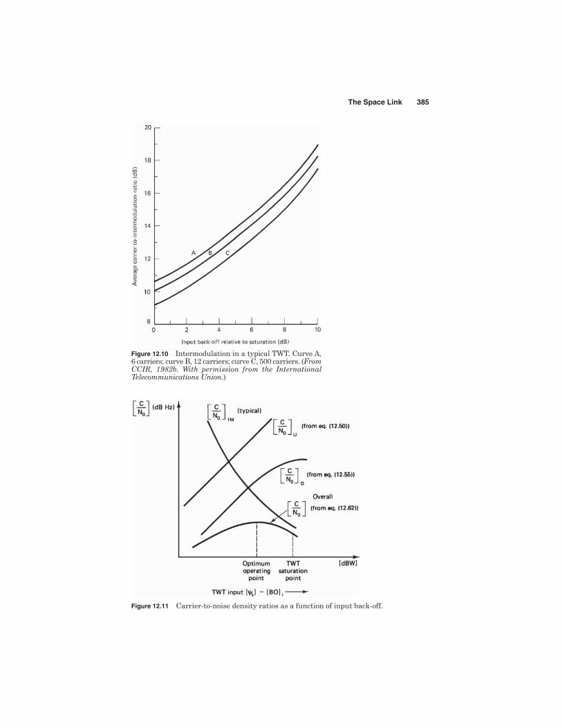
The Space Link 385
Figure 12.11 Carrier-to-noise density ratios as a function of input back-off.
Figure 12.10 Intermodulation in a typical TWT. Curve A,6 carriers; curve B, 12 carriers; curve C, 500 carriers. (FromCCIR, 1982b. With permission from the InternationalTelecommunications Union.)

ground stations. Although many different links are possible, the mostuseful ones in operation are:
low earth orbiting (LEO) satellites—LEO ↔ LEO geostationary earth orbiting (GEO) satellites—GEO ↔ GEO LEO ↔ GEO
Consider first some of the applications to GEOs. As shown in Chap.3, the antenna angle of elevation is limited to a minimum of about 5degrees because of noise induced from the earth. The limit of visibilityas set by the minimum angle of elevation is a function of the satellitelongitude and earth-station latitude and longitude as shown in Sec. 3.2.Figure 12.12 shows the situation where earth station A is beyond therange of satellite S2, a problem that can be overcome by the use of twosatellites connected by an ISL. Thus, a long distance link between earthstations A and B can be achieved by this means. A more extreme exam-ple is where an intercontinental service may require a number of “hops.”For example a Europe-Asia circuit requires three hops (Morgan, 1999):Europe to eastern U.S.A; eastern U.S.A. to western U.S.A; westernU.S.A. to Asia; and of course each hop required an uplink and a down-link. By using an ISL only one uplink and one downlink is required. Also,as will be discussed shortly, the ISL frequencies are well outside thestandard uplink and downlink bands so that spectrum use is conserved.The cost of the ISL is more than offset by not having to provide the addi-tional earth stations required by the three-hop system.
The distance d for the ISL is easily calculated. From Fig. 12.13:
(12.63)
where is the longitudinal separation between satellites S1 and S2,and aGSO is the radius of the geostationary orbit [see Eq. (3.2)], equal to42164 km. For example the western limits for the continental UnitedStates (CONUS) arc are at 55° and 136° (see Prob. 3.11). Although thereare no satellites positioned exactly at these longitudes they can be used
d 2aGSO sin
2
386 Chapter Twelve
S1 S2d
A B
El2El1
El1 < Elmin < El2
Figure 12.12 Angle of elevation as determined by an ISL.

to get an estimate of distance d for an ISL spanning CONUS.
Although this may seem large, the range from earth station to satel-lite is in the order of 41000 km, (Prob. 3.11) so distance involved withthree uplinks and three downlinks is 246000 km!
GEO satellites are often arranged in clusters at some nominal longitude.For example, there are a number of EchoStar satellites at longitude 119°W.The separation between satellites is typically about 100 km, the corre-sponding longitudinal separation for this distance being, from Eq. (12.63),approximately 0.136°. Because the satellites are relatively close togetherthey are subject to the same perturbing and drift forces which simplifiespositional control. Also, all satellites in the cluster are within the main lobeof the earth-station antenna.
Because LEO satellites are not continuously visible from a given earthlocation, an intricate network of satellites is required to provide contin-uous coverage of any region. A typical LEO satellite network will utilizea number of orbits, with equispaced satellites in each orbit. For exam-ple, the Iridium system uses 6 orbital planes with 11 equispaced satel-lites in each plane, for a total of 66 satellites. Communication betweentwo earth stations via the network will appear seamless as messagehandover occurs between satellites via intersatellite links.
Radio frequency ISLs make use of frequencies that are highly atten-uated by the atmosphere, so that interference to and from terrestrial sys-tems using the same frequencies is avoided. Figure 4.2 shows theatmospheric absorption peaks at 22.3 GHz and 60 GHz. Table 12.3shows the frequency bands in use:
d 2 42164 sin
(136 55)
2 54767 km
The Space Link 387
S2
S1
aGSO
aGSO
d
2–
Δf2—
Figure 12.13 Finding the distance d betweentwo GEO satellites.
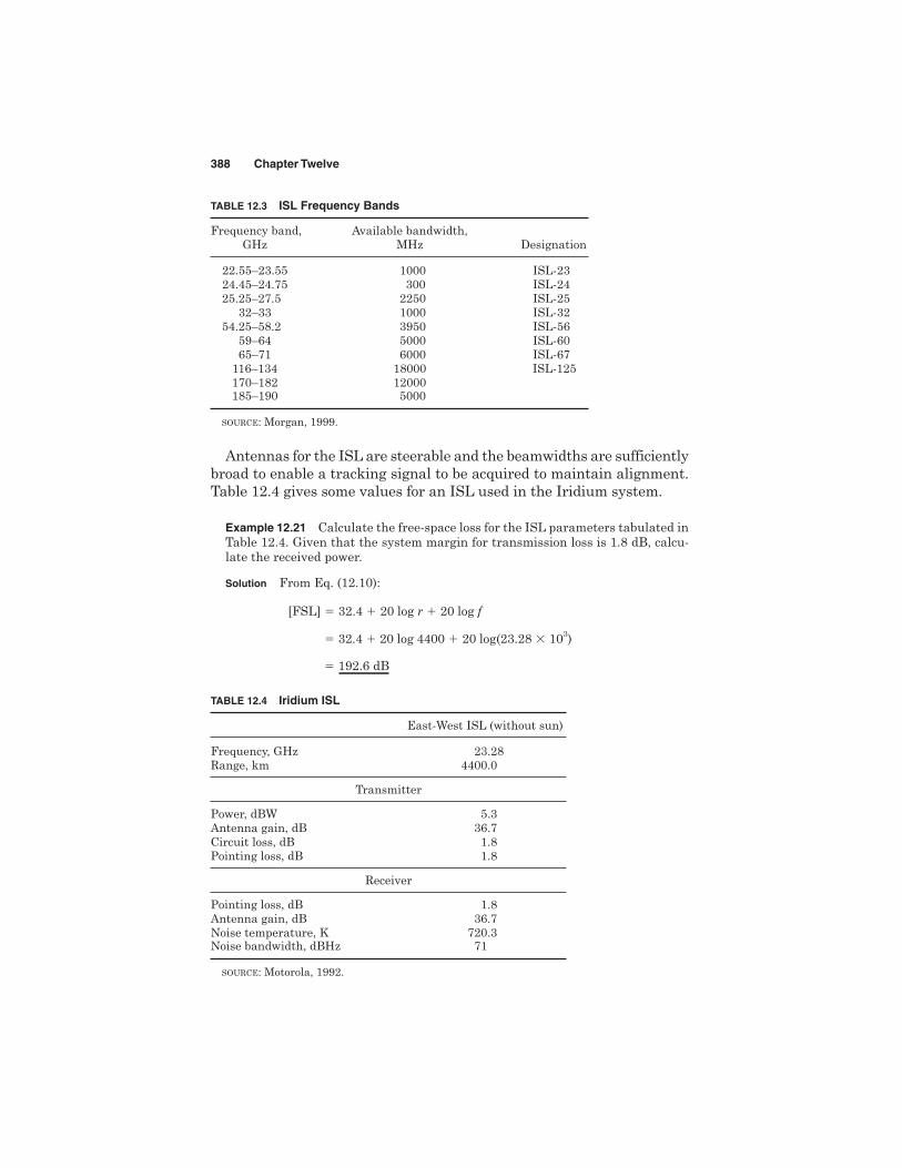
Antennas for the ISL are steerable and the beamwidths are sufficientlybroad to enable a tracking signal to be acquired to maintain alignment.Table 12.4 gives some values for an ISL used in the Iridium system.
Example 12.21 Calculate the free-space loss for the ISL parameters tabulated inTable 12.4. Given that the system margin for transmission loss is 1.8 dB, calcu-late the received power.
Solution From Eq. (12.10):
[FSL] 32.4 20 log r 20 log f
32.4 20 log 4400 20 log(23.28 103)
192.6 dB
388 Chapter Twelve
TABLE 12.3 ISL Frequency Bands
Frequency band, Available bandwidth,GHz MHz Designation
22.55–23.55 1000 ISL-2324.45–24.75 300 ISL-2425.25–27.5 2250 ISL-25
32–33 1000 ISL-3254.25–58.2 3950 ISL-56
59–64 5000 ISL-6065–71 6000 ISL-67
116–134 18000 ISL-125170–182 12000185–190 5000
SOURCE: Morgan, 1999.
TABLE 12.4 Iridium ISL
East-West ISL (without sun)
Frequency, GHz 23.28Range, km 4400.0
Transmitter
Power, dBW 5.3Antenna gain, dB 36.7Circuit loss, dB 1.8Pointing loss, dB 1.8
Receiver
Pointing loss, dB 1.8Antenna gain, dB 36.7Noise temperature, K 720.3Noise bandwidth, dBHz 71
SOURCE: Motorola, 1992.

The [EIRP] is
[EIRP] [PT] [GT] [AML]T [TFL]
5.3 36.7 1.8 1.8
38.4 dBW
The total losses, including the link margin and the receiver misalignment (point-ing) loss are:
[LOSSES] 192.6 1.8 1.8 196.2 dB. The received power is, from Eq. (12.13)
[PR] [EIRP] [GR] [LOSSES]
121.1 dBW
Radio ISLs have the advantage that the technology is mature, so therisk of failure is minimized. However, the bandwidth limits the bit ratethat can be carried, and optical systems, with their much higher carrier(optical) frequencies, have much greater bandwidth. Optical ISLs havea definite advantage over rf ISLs for data rates in excess of about 1 GbpsAlso, telescope apertures are used which are considerably smaller thantheir rf counterparts, and generally, optical equipment tends to be smallerand more compact (see Optical Communications and IntersatelliteLinks,undated, at www.wtec.org/loyola/satcom2/03_06.htm-22k-). The opticalbeamwidth is typically 5 rad (Maral et al., 2002). Table 12.5 lists prop-erties of some solid state lasers.
The free-space loss given by Eq. (12.9) is repeated here:
[FSL] 10 loga4rl b
2
The Space Link 389
TABLE 12.5 Solid State Lasers
Wavelength, Beam diameter,Type m Power mm Beam divergence
GaAs/GaAlAs 0.78–0.905 1–40 mW Avg 10° 35°InGaAsP 1.1–1.6 1–10 mW 10° 30° 20°
40°Nd: YAG 1.064 Up to 600 W Avg 1– 10 0.3–20 mrad
PulsedNd:YAG Diode 1.064 0.5–10 mW 1–2 0.5–2.0 mrad
pumpedNd:YAG (cw) 1.064 0.04–600 W 0.7–8 2–25 mrad
NOTES: Al—aluminum; As—arsenide; Ga—gallium; Nd—neodymium; P— phosphorus;YAG—yttrium-aluminum garnet; cw—continuous wave; m—micron = 106 m; mm—millimeter; mrad—milliradian; mW—milliwatt; W—watt.
SOURCE: Extracted from Chen, 1996.

Here, wavelength rather than frequency is used in the equation as thisis the quantity usually specified for a laser, and of course r and l mustbe in the same units.
The intensity distribution of a laser beam generally follows what istermed a Gaussian law, for which the intensity falls off in an exponen-tial manner in a direction transverse to the direction of propagation. Thebeam radius is where the transverse electric field component drops to1/e of its maximum value, where e ≈ 2.718. The diameter of the beam(twice the radius) gives the total beamwidth. The on-axis gain (similarto the antenna gain defined in Sec. 6.6 is given by (Maral et al., 2002)
(12.64)
where T is the total beamwidth.On the receive side, the telescope aperture gain is given by:
(12.65)
where D is the effective diameter of the receiving aperture.The optical receiver will receive some amount of optical power PR. The
energy in a photon is hc/l, where h is Plank’s constant (6.6256 1034
J-s) and c is the speed of light in vacuum (approximately 3 108 m/s).For a received power PR the number of photons received per second istherefore PRl/hc. The detection process consists of photons impartingsufficient energy to valence band electrons to raise these to the con-duction band. The quantum efficiency of a photo-diode is the ratio (aver-age number of conduction electrons generated)/(average number ofphotons received). Denoting the quantum efficiency by , the averagenumber of electrons released is PRl/hc and the photo current is:
(12.66)
where q is the electron charge. The responsivity of a photodiode is definedas the ratio of photo current to incident power. Denoting responsivityby R0 and evaluating the constants in Eq. (12.66) gives
(12.67)
The energy band gap of the semiconductor material used for the pho-todiode determines the wavelengths that it can respond to. The require-ment in general is that the bandgap energy must be less than the photon
R0 l
1.24 with l in m
Iph qPRl
hc
GR aDl b
2
GT 32T
2
390 Chapter Twelve

energy, or EG < hc/l. On this basis it turns out that silicon is useful forwavelengths shorter that 1 m. Germanium is useful at 1.3 m and InSband InAs at 1.55 m.
The total current flowing in a photodiode consists of the actual cur-rent generated by the photons, plus what is termed the dark current.This is the current that flows even when no signal is present. Ideally itshould be zero, but in practice it is of the order of a few nanoamperes,and it can contribute to the noise. Denoting the dark current by Id thetotal current is
(12.68)
This current is accompanied by shot noise (a name that is a hangoverfrom vacuum tube days), the mean square spectral density of which is2qI in A2/Hz with I in amperes. This would be for a diode without anyinternal amplification such as a PIN diode. An avalanche photo diode(APD) multiplies the signal current by a factor M and at the same timegenerates excess noise, represented by an excess noise factor, F, so thatthe mean square spectral density is (2qI)MF. F increases with increasein M (see Jones, 1988, p. 240). Typical values are of the order M 100,F 12. For a PIN diode, M 1 and F 1.
The analysis to follow is based on that given in Jones (1988). Theequivalent circuit for the input stage of an optical receiver is shown inFig. 12.14, where R is the parallel combination of diode resistance, inputload resistance and preamplifier input resistance, and C is the parallelcombination of diode capacitance, preamplifier input capacitance andstray circuit capacitance. Resistance R will generate thermal noise cur-rent, the spectral density of which is 4kT/R (k is Boltzmann’s constantand T is the temperature, which may be taken as room temperature).The preamplifier transistor will also generate shot noise, which when
I Iph Id
The Space Link 391
isR Ci2t
V2a
Figure 12.14 The equivalent input circuit for an optical receiver. it2
is the mean square spectral density for the current noise source, andva
2 the mean square spectral density for the voltage noise source. isis the signal current.

referred to the input has a spectral density 2q/Iin in A2/Hz, where Iin isthe transistor gate (JFET) or base (BJT) current in amperes. Usingcurly brackets . for the spectral density values (see Jones, 1988), thetotal noise current spectral density at the input is
(12.69)
The pre-amplifier also has a noise voltage component shown as va
resulting from the shot noise in the drain or collector current. The meansquare noise voltage spectral density is 2qItr/g
2mV2/Hz where Itr is the
transistor drain (JFET) or collector (BJT) current in amperes and gm isthe device transconductance in siemens. The total noise voltage spec-tral density at the input is therefore
(12.70)
where ZL is the impedance of R and C in parallel.The average signal voltage is MIphR. Increasing R should result in an
increase in signal to noise ratio since the signal voltage is proportionalto R and the R component of noise current density is inversely propor-tional to R. However, the bandwidth of the RC input network is inverselyproportional to R and therefore sets a limit to how large R can be. Anequalizing filter, which has a transfer function, given by
can be included in the overall transfer function,which compensates for the input impedance frequency response over thesignal bandwidth. The effective spectral density for the mean squarenoise voltage at the input is then . The mean square noisevoltage Vn
2 at the input is obtained by integrating this expression overthe signal bandwidth. Only the result will be given here:
(12.71)
With the average signal voltage given by Vs MIphR the signal to noiseratio is
(12.72)
(MIphR)2
c a2qIM2F 4kTR
2qIinbR2
2qItr
gm2 a1
(2RCB)2
3b dB
SN
Vs
2
Vn2
Vn2
c a2qIM2F
4kTR
2qItrbR2
2qItr
gm2 a1
(2RCB)2
3b dB
5vn26 ZH( f ) Z2
Heq(f) 1 j2 f RC
5vn26 5 5it
26 ZZL Z21
2qItr
gm2 V2/Hz
5it26 5 2qIM2F1
4kTR1 2qItr A2/Hz
392 Chapter Twelve

This can be simplified on dividing through by M2R2 to get:
(12.73)
Example 12.22 An optical receiver utilizes an APD for which R0 0.65 A/W,M 100, F 4, Iin 0, gm 3000 mS and Itr 0.15 mA. The dark current maybe neglected. The input load consists of a 600 Ω resistor in parallel with a 10pFcapacitance. The signal bandwidth is 25 MHz and equalization is employed.Calculate the resultant signal-to-noise ratio for an input signal power of 1 W.
Solution The photocurrent is Iph 0.65 106 0.65 A. The individual terms
in the denominator are, with Id 0 and Iin 0:
2.622 104
In decibels this is 44.2 dB
12.13 Problems and Exercises
Note: In problems where room temperature is required, assume a value of 290K. In calculations involving antenna gain, an efficiency factor of 0.55 may beassumed.
12.1. Give the decibel equivalents for the following quantities: (a) a powerratio of 30:1; (b) a power of 230 W; (c) a bandwidth of 36 MHz; (d) a frequencyratio of 2 MHz/3 kHz; (e) a temperature of 200 K.
12.2. (a) Explain what is meant by EIRP. (b) A transmitter feeds a power of10 W into an antenna which has a gain of 46 dB. Calculate the EIRP in (i) watts;(ii) dBW.
12.3. Calculate the gain of a 3-m parabolic reflector antenna at a frequency of(a) 6 GHz; (b) 14 GHz.
S
N
(0.65 106)2 1025
(6.408 0.027 0.011) 25 106
2qItr
M 2gm2a 1
R2
(2CB)2
3b 0.011 1025 A2/Hz
4kT
M 2R 0.027 1025 A2/Hz
2qIF 6.408 1025 A2/Hz
SN
Iph
2
c2qIF 4kTM2R
2qIin
M2
2qItr
M2gm2 a 1
R2
(2CB)2
3b dB
The Space Link 393


![RSS-170 [Satellite Mobile Earth Stations]](https://static.fdocuments.in/doc/165x107/577d274a1a28ab4e1ea38a47/rss-170-satellite-mobile-earth-stations.jpg)


