DRAFT – Please do not cite without permission

July 18, 2008

The Distributional Effects of the Social Security

Windfall Elimination Provision

Jeffrey R. Brown

University of Illinois and NBER

and

Scott Weisbenner

University of Illinois and NBER

Prepared for the 10th Annual Joint Conference of the Retirement Research Consortium

“Determinants of Retirement Security”

August 7-8, 2008

Washington, D.C.

The research reported herein was pursuant to a grant from the U.S. Social Security

Administration (SSA) funded as part of the Retirement Research Consortium (RRC).

The findings and conclusions expressed are solely those of the authors and do not

represent the views of SSA, any agency of the Federal Government the RRC or the

NBER. We are grateful to Steve Goss and Bert Kestenbaum for providing us with data

and for helpful discussions. We thank Chichun Fang for excellent research assistance.

Abstract: Millions of federal, state and local government employees have lifetime earnings that are divided between employment that is covered by the Social Security system and employment that is not covered. Because Social Security benefits are a non-linear function of covered lifetime earnings, the simple application of the standard benefit formula to covered earnings only would provide a higher replacement rate on those earnings than is appropriate given the individuals’ total (covered plus uncovered) lifetime earnings. The Windfall Elimination Provision (WEP), established in 1983, is intended to correct this situation by applying a modified benefit formula to earnings of individuals with non-covered employment. This paper analyzes the distributional implications of the WEP, and finds that it reduces benefits disproportionately for households with lower lifetime covered earnings. It discusses an alternative method of calculating the WEP that preserves the intended redistribution of the system. In recognition of the data limitations that prevent this alternative method from being used by SSA for at least another decade, the paper also explores two alternative ways of calculating the WEP that use the same information that SSA currently uses, are budget neutral, and do a better job of maintaining progressivity than the current WEP formula.

1. Introduction

Approximately one fourth of all public employees in the U.S. do not pay Social

Security taxes on the earnings from their government job (U.S. GAO, 2007). This

includes approximately 5.25 million state and local workers, as well as approximately 1

million federal employees hired before 1984 (U.S. GAO, 2003). Many of these public

employees still qualify for Social Security benefits, either as a result of switching

between covered and uncovered employment at some point in their career or because

they simultaneously work two or more jobs that span both covered and uncovered

employment. For example, a teacher in the State of Illinois (one of the states whose

public workers are not covered under Social Security) may spend his summers working

in covered employment. Alternatively, a professor may spend part of her career working

at a private university covered by Social Security, and part of her career working for a

state university that is not covered.

If Social Security benefits were calculated as a simple linear function of lifetime

earnings, it would be possible to calculate the retirement benefit for a worker with partial

coverage by simply applying the standard benefit formula only to those earnings covered

by Social Security. However, Social Security’s benefit formula was explicitly designed

to be non-linear in order to offer a higher replacement rate (e.g., a higher ratio of Social

Security benefits to average indexed monthly earnings over one’s lifetime) for

individuals with lower earnings. For workers employed by certain federal, state, or local

governments who have earnings that are not covered by the Social Security system, using

only covered earnings in the standard benefit formula would result in a higher

“replacement rate” on these covered earnings than they would receive if all of their

earnings were covered.

In order to adjust for this, the Windfall Elimination Provision (WEP) was enacted

as part of the 1983 Social Security Amendments. This provision is meant to downward-

adjust the Social Security benefits of affected workers in order to eliminate the “windfall”

that arises when, for example, an individual with high lifetime earnings (based on both

covered and uncovered earnings) would appear as if he or she were a low earner when

evaluated solely based on covered earnings.

The WEP is extremely controversial to those affected by it. Indeed, bills to

eliminate or alter the WEP are regularly proposed in Congress.1 There are numerous

potential reasons for the intense opposition to the WEP by those affected, including that:

(a) the underlying rationale for the WEP does not appear to be well-understood by many

of those affected by it, (b) the official SSA publications quite clearly frame the WEP as a

benefit cut, and (c) the WEP is perceived as being particularly unfair to lower income

individuals. This paper discusses all three of these concerns, although the primary

contribution is to investigate the third claim by analyzing the distributional implications

of the WEP in comparison to several alternative methods of calculating this adjustment.

We find that the WEP does indeed reduce benefits disproportionately for lower

earning households than for higher earning households. Because the WEP changes the

marginal Social Security benefit only on the first $711 (in 2008) of average indexed

monthly earnings, the WEP reduces benefits by a larger percentage for households with

lower covered earnings. Because the WEP provision is phased out for individuals with

20 to 30 years of sufficient covered earnings (to be explained in more detail below), the

WEP provision can also, in some cases, lead to large changes in Social Security

replacement rates based on small changes in covered earnings. This potentially has both

distributional and labor supply incentive effects.

1 In the 110th Congress, such bills include the “Public Servant Retirement Protection Act of 2007” (H.R. 2772 and S. 1647). These bills often garner a large number of co-sponsors, especially from states whose state employees are affected by these provisions.

2

This paper begins in section 2 by describing in more detail why an adjustment for

uncovered earnings is appropriate. In section 3, we discuss the details of the WEP

calculation as it is currently applied. In section 4, we discuss the distributional

implications of the WEP as currently applied. In section 5 we present two alternative

methods for calculating the WEP that are administratively feasible and that may do a

better job of preserving the income progressivity that is inherent in the broader Social

Security system. Section 6 provides a very brief overview of a distinct but related

provision – the Government Pension Offset. Section 7 draws conclusions and provides

further commentary on the WEP, including a brief discussion of how the framing of the

existing WEP adjustment likely exacerbates the political unpopularity of this provision.

2. Why is a Benefit Adjustment Necessary for Government Employees?

A brief review of how Social Security benefits are calculated provides a useful

background for understanding the need for a benefit adjustment for workers with both

covered and uncovered earnings. Let’s begin with an individual born in 1946, who will

turn age 62 in the year 2008, and whose earnings are 100 percent covered, as is the case

with most employees in the U.S. This individual’s earnings in each year are first indexed

to the average wage index to bring nominal earnings up to near-current wage levels.2

Social Security then averages the highest 35 years of indexed earnings and divides by 12

to compute the Average Indexed Monthly Earnings (AIME).

The next step is to compute the Primary Insurance Amount (PIA), which is the

basis for all benefit calculations. For the 1946 birth cohort, the PIA is calculated as a

function of the AIME as follows:

( ) ( )( )( )4288,0max15.0

7114288,min,0max32.0711,min9.0

−⋅+

−⋅+⋅=

AIME

AIMEAIMEPIA WEPNo (1)

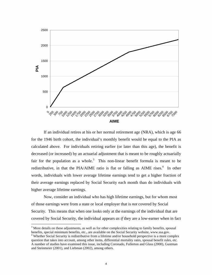
The benefit formula in equation 1 is most easily scene graphically:

Figure 1: The Social Security Benefit Formula (1946 birth cohort)

2 The indexing factor for a prior year is the result of dividing the average wage index (AWI) for the year in which the person attains age 60 by the average wage index for year Y. A factor will always equal one for the year in which the person attains age 60 and all later years. http://www.socialsecurity.gov/OACT/ProgData/retirebenefit1.html

3

0

500

1000

1500

2000

2500

025

050

075

010

0012

5015

0017

5020

0022

5025

0027

5030

0032

5035

0037

5040

0042

5045

0047

5050

0052

5055

0057

5060

0062

5065

0067

5070

00

AIME

PIA

If an individual retires at his or her normal retirement age (NRA), which is age 66

for the 1946 birth cohort, the individual’s monthly benefit would be equal to the PIA as

calculated above. For individuals retiring earlier (or later than this age), the benefit is

decreased (or increased) by an actuarial adjustment that is meant to be roughly actuarially

fair for the population as a whole.3 This non-linear benefit formula is meant to be

redistributive, in that the PIA/AIME ratio is flat or falling as AIME rises.4 In other

words, individuals with lower average lifetime earnings tend to get a higher fraction of

their average earnings replaced by Social Security each month than do individuals with

higher average lifetime earnings.

Now, consider an individual who has high lifetime earnings, but for whom most

of those earnings were from a state or local employer that is not covered by Social

Security. This means that when one looks only at the earnings of the individual that are

covered by Social Security, the individual appears as if they are a low-earner when in fact 3 More details on these adjustments, as well as for other complexities relating to family benefits, spousal benefits, special minimum benefits, etc., are available on the Social Security website, www.ssa.gov. 4 Whether Social Security is redistributive from a lifetime and/or household perspective is a more complex question that takes into account, among other items, differential mortality rates, spousal benefit rules, etc. A number of studies have examined this issue, including Coronado, Fullerton and Glass (2000), Gustman and Steinmeier (2001), and Liebman (2002), among others.

4

they are a high-earner. Applying the benefit formula in equation 1 only to covered

earnings would place this person on the high replacement rate portion of the benefit

formula, in essence giving this individual too large of a benefit relative to their total

(covered plus uncovered) lifetime earnings.

It is easiest to see the problem that would be created if there were no WEP

provision in place through an example. Consider the three individuals shown in Table 1.

Person A is a very low income worker who works her entire life under Social Security,

with an AIME of only $500 per month. Using the 2008 PIA formula (applicable to the

1946 birth cohort, as it appears in equation 1 above), person A would have a PIA of $450,

or a replacement rate of 90%. Person B is a higher income worker with all of her

earnings covered under Social Security, thus having an AIME of $5,000. Applying

equation 1 indicates that Person B would have a PIA of $1891.34, or a replacement rate

at the NRA of nearly 38%. Thus far, this example simply illustrates the non-linearity of

the benefit formula, as person A receives a higher replacement rate than does person B,

owing to the fact that person A has lower lifetime earnings.

Table 1 Social Security Primary Insurance Amount If No WEP Adjustment Applied

AIME of covered earnings

AIME of non-covered earnings

AIME of total earnings

PIA if standard formula applied to covered earnings

PIA / AIME of covered earnings with no WEP adjustment

Person A 500 0 500 450 90%

Person B 5000 0 5000 1891 38%

Person C 500 4500 5000 450 90%

Now consider person C, a public employee. Person C’s total lifetime earnings

(which on an indexed average monthly basis were $5,000) are identical to B’s. Had all of

person C’s earnings been covered by Social Security, person C would have the same 38%

replacement rate as B. However, only 1/10th of person C’s earnings were in employment

covered by Social Security; the rest were in non-covered public employment. If Social

Security applied the standard benefit formula to person C’s covered earnings without any

WEP adjustment, person C would receive a monthly benefit of $450, equivalent to person

5

A. This provides person C with a ratio of PIA to (covered) AIME of 90%, which is

substantially more generous than the 38% ratio provided to person B, even though B and

C have identical lifetime earnings. To use the language of the provision designed to

address this issue, person C would receive a “windfall.”

3. How Does the WEP Work?

In 1983, Congress acted to correct this potential “windfall” to public employees.

A natural approach to adjusting for public employment, which we will call the

“proportional WEP” to distinguish it from the actual WEP, would entail calculating a

participant’s “total PIA” based on total (covered and non-covered earnings) – $1891.34

in the case of person C – and then multiplying by the ratio of covered-to-total earnings –

0.1 for person C. This would result in a “covered PIA” of $189.13. Note that the

resulting replacement rate of covered earnings under the “proportional WEP” is, by

construction, 38%, identical to the replacement rate provided to an individual with

identical total lifetime earnings. In addition to preserving the distributional aspect of the

benefit formula, this approach would also be relatively simple to explain to affected

participants in a manner that would likely be viewed as “fair.”5

Implementation of a proportional WEP, however, would require that SSA keep

track of total earnings, including non-covered earnings. Unfortunately, this could not be

operationalized by the Social Security Administration in 1983 due to the fact that the

SSA had not historically collected information on non-covered earnings. Specifically,

according to recent Congressional testimony by an SSA official, “SSA only has records

of non-covered earnings beginning in 1978, when it began receiving Form W-2

information from employers, and some of these records are incomplete – particularly for

the years soon after SSA began collecting this earnings information” (Social Security

Administration, 2005). Even if one assumes that the SSA records became more complete

by the time of the 1983 amendments that introduced the WEP provision, it will be

another decade before SSA has at least 35 years of both covered and uncovered earnings

for new retirees. It will be several years beyond that before SSA can produce

5 For example, SSA could simply state that “over your lifetime, 10% of your earnings were subject to the Social Security payroll tax. Thus, you will receive 10% of the benefit that you would have received had you paid taxes on all of your earnings.”

6

proportional WEP computations based on a complete earnings history. Diamond and

Orszag (2003) have suggested that this approach could be implemented now by requiring

that this alternative calculation “be available only to workers who provide the Social

Security Administration with a complete history of earnings in non-covered work.” Such

an approach would increase benefit expenditures, however, as only those workers who

would see their benefit rise as a result of the alternative calculation would have the

incentive to provide such records.

In recognition of these operational constraints, Congress created a modified

benefit formula that is based only on covered earnings. The key difference between the

ordinary benefit formula and the one used for individuals subject to the WEP is that

under the WEP, the covered earnings up to the first PIA bend point (e.g., the first $711 of

AIME in the year 2008) are converted to PIA at a rate of 0.4 rather than 0.9. Note that

the WEP adjustment is applied to the PIA before benefits are adjusted for early claiming,

delayed claiming, or cost of living adjustments. Because this applies only on the first

$711 of AIME, the maximum benefit reduction under the WEP is $355.50 per month, or

$4,266 per year, in 2008.

This formula is then further altered for individuals who have more than 20 years

of “years of coverage” (YOC), defined as any year in which an individual has covered

earnings that meet a minimum amount. For the year 2008, a YOC is defined as earnings

in excess of $18,975.6 For individuals with 20 or fewer YOCs, earnings to the first PIA

formula bend point are credited at 0.4. For each year over 20, the first PIA factor is

increased by an additional 0.05. For individuals with 30 or more years of YOCs, the

benefit formula is identical to the standard, non-WEP adjusted benefit formula.

Formally, the benefit formula for individuals affected by the WEP can be represented as:

( )( )( ) ( )( )( ) ( )4288,0max15.07114288,min,0max32.0

711,min20,0max,10min05.04.0−⋅+−⋅+

⋅−⋅+=AIMEAIME

AIMEYOCPIAWEP (2)

Thus, for person C in the example above who had a covered AIME of $500, the

PIA after the WEP adjustment (assuming fewer than 20 YOCs) would be $200, for a

6 “For 1951-78, the amount of Social Security covered earnings needed for a year of coverage is 25 percent of the contribution and benefit base. For years after 1978, the amounts are 25 percent of what the contribution and benefit based would have been if the 1977 Social Security Amendments had not been enacted.” http://www.socialsecurity.gov/OACT/COLA/yoc.html

7

PIA/AIME “replacement rate” on covered earnings of 40%. The fact that the benefit

calculated under the actual WEP formula differs from the proportional WEP described

above is typically the rule rather than the exception.

These adjustments can be seen in Figure 2, which shows the benefit formula for

an individual with 30+ YOCs (or, identically, someone not subject to the WEP), an

individual with 25 YOCs, and an individual with 20 or fewer YOCs.

Figure 2: The PIA Formula with WEP Adjustments

0

500

1000

1500

2000

2500

025

050

075

010

0012

5015

0017

5020

0022

5025

0027

5030

0032

5035

0037

5040

0042

5045

0047

5050

0052

5055

0057

5060

0062

5065

0067

5070

00

AIME

PIA

PIA PIA WEP (25 YOCS) PIA WEP (<=20 YOCs)

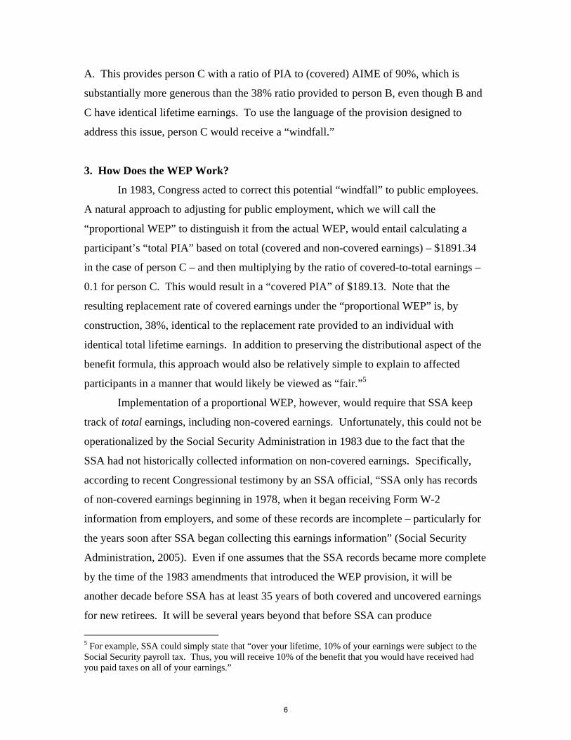
4. Distributional Implications of the WEP

There are two aspects of the WEP adjustment that cause it to potentially affect

low earners proportionately more than higher earners. First, the maximum WEP

adjustment is reached at a low level of earnings: specifically, the WEP reduction applies

only to covered earnings up to the first PIA bend-point ($711 in 2008). For all

individuals with covered AIME above this, the maximum reduction of $355.50 represents

a smaller fraction of earnings as earnings rise. This simple point is illustrated in Figure 3,

which charts the replacement rate (the ratio of PIA at the NRA relative to covered AIME)

8

for different income levels for individuals with no WEP (or individuals with 30+ YOCs)

and for individuals with 20 or fewer YOCs who are subject to the WEP.

Figure 3: Covered Earnings Replacement Rates With and Without WEP

0

0.1

0.2

0.3

0.4

0.5

0.6

0.7

0.8

0.9

1

050

010

0015

0020

0025

0030

0035

0040

0045

0050

0055

0060

0065

0070

00

Covered AIME

PIA

/ C

over

ed A

IME WEP (<20 YOCs) No WEP

The difference between the two lines is the result of the WEP, and not

surprisingly, this adjustment is larger (relative to covered AIME) for those with a lower

AIME. Thus, holding constant the fraction of total earnings that are covered, the WEP

hits lower earners proportionally harder.

A second way in which the WEP can have a distributional impact can be seen

when one holds constant the fraction of earnings covered, and instead varies total

(covered plus uncovered) earnings. Recall that a YOC is granted for a given year on an

all-or-nothing basis, depending on whether one’s covered earnings exceed the threshold.

Thus, if we hold constant the fraction of total income that is covered versus uncovered, a

higher income individual is more likely to cross the YOC threshold. For example, if two

individuals each have 50 percent of their earnings covered, the person who earns $40,000

per year has covered earnings ($20,000) that exceed the YOC threshold in 2008, while an

9

individual earning $35,000 per year has covered earnings ($17,500) that are below the

threshold.

For individuals close to the YOC in a given year who expect to have between 20

and 30 YOCs in their lifetime, crossing the YOC threshold can boost lifetime benefits

substantially. For example, an individual claiming in 2008 with an AIME exceeding

$711 (so that the full WEP offset applies), increasing one’s YOCs by one year (between

20 and 30) would boost initial individual benefits at the NRA by $35.55 per month.

Given that these benefits are inflation indexed and last for life, the increment to the

expected present value of lifetime benefits (calculated as of the NRA) is over $5,000 for

each additional YOC between 20 and 30.7 Indeed, the increment to lifetime income

would be even higher for those receiving spousal, survivor, and other family benefits that

are calculated based on this PIA.

Another way to view the magnitude of this change is as follows. For someone

whose AIME is between the two bend points (i.e., between $711 and $4288), raising

one’s PIA by $35.50 per month would normally require raising one’s lifetime earnings

(on a wage indexed basis) by $46,593.75.8 For an individual with an AIME beyond the

2nd bend point, the increment to lifetime earnings required to boost monthly income by

$35.50 is $99,400. Yet for those in the affected range of the WEP, this incremental

benefit can be earned by having only $18,975 in covered earnings during the year. Thus,

in addition to distributional effects being explored here, these provisions could have large

effects on labor supply incentives for individuals in the affected range.

The full WEP formula, including the YOC adjustment, can lead to some highly

non-linear movements in the benefit-to-AIME ratio as the fraction of covered earnings

rises. For example, in Figure 4, we use an individual classified by the SSA actuaries as a

“maximum earner,” i.e., an individual whose earnings in every year were precisely equal

to the maximum earnings that were subject to the payroll tax in that year. We assume

this individual enters the workforce at age 21 in 1967, and retires and claims on his 62nd

birthday (assumed to be 1/1/08). Because the individual is claiming before his normal 7 The present value calculation assumes a unisex mortality table and a real interest rate of 3%. 8 $46,593.75 = (35.50 / 0.32) * 12 * 35. In words, the extra $35.50 in monthly benefits for an individual on the middle bend point factor requires an additional $110.94 per month of AIME. This is $1,332.25 annually. Because the benefit formula is based on the 35 highest years, this requires a boost in lifetime indexed earnings of $46,593.75.

10

retirement age, the benefit that he receives by claiming on 1/1/08 is approximately 75%

of his PIA.9

Figure 4: Ratio of Benefit at Age 62 to Covered AIME for “Max Earner”

0.00%

10.00%

20.00%

30.00%

40.00%

50.00%

60.00%

70.00%

80.00%

0 5 10 15 20 25 30 35 40 45 50 55 60 65 70 75 80 85 90 95 100

Percentage of Earnings Covered by Social Security

Rat

io o

f Age

62

Ben

efit

to C

over

ed A

IME Proportional WEP Cov. Earnings Only w/o WEP Cov. Earnings Only w/ WEP

In the figure, we vary the fraction of total earnings that are covered by Social

Security from 0% to 100%, in each case assuming that this percentage applies to earnings

in every individual year. There are three lines presented in Figure 4. For comparison, the

horizontal line at just under 24% is the replacement rate that a max earner would receive

at ate 62 under the “proportional WEP” baseline. Recall that this proportional WEP is a

useful baseline because it replicates the replacement rate that the person would receive if

100% of their earnings were fully covered by Social Security.

The second line, which begins at just under 68% (which corresponds to the 90%

PIA factor, adjusted by the age 62 actuarial reduction) and then gradually declines to the

24% rate when all earnings are covered, is the replacement rate that the max earner would

receive if there were no WEP adjustment. The difference between these first two lines is 9 With a January 1 birthday, the SSA treats the individual as if they were born the prior month. Thus, beginning entitlement in January 2008 causes this individual to be treated as if they claimed at age 62 and one month. Therefore, the precise actuarial adjustment for this individual results in an initial benefit that is 75.42% of his PIA.

11

a measure of the “windfall” that the WEP was meant to address. The third line shows the

replacement rate provided under the actual WEP formula.

There are three noteworthy points about the actual WEP benefit pattern relative to

the “No WEP” and “WEP” benefits. The first and most obvious point, which is true

based on how the WEP is calculated, is that all the replacement rates with the WEP are

lower than or equal to those resulting from the application of the standard PIA formula to

covered earnings without regard for the windfall. A second point to note is that, for this

maximum earner, the replacement rates are all higher than the 24% that the individual

would have received under a proportional WEP. In other words, maximum earners are

getting a better return on their Social Security dollars – even with the WEP adjustment –

than they would receive had their earnings been fully covered by Social Security. Thus,

it is somewhat ironic that these individuals would find the WEP so objectionable, given

that the current design of the WEP still provides them with a higher replacement rate on

their covered earnings than otherwise similar lifetime earners are receiving.

A third point to note about this line is that the pattern of replacement rates is

highly non-monotonic. It begins at approximately 30% (which corresponds to the 40%

PIA factor under the WEP, adjusted by the age 62 actuarial reduction)) when 10% or less

of earnings each year are in covered employment, and then gradually drops to 27.4%

before jumping up to over 40%, and then declining gradually. The discrete jumps occur

at places where a small change in the fraction of covered earnings each year causes the

individual’s covered earnings in some years to qualify as YOCs. For example, the move

from 19 to 20% of earnings causes a jump from 2 to 27 in the number of years of this

particular earnings profile where the YOC threshold is met, thus increasing the first PIA

factor from 0.4 to 0.75 (such a disproportionate jump is admittedly an artifact of how

these particular earnings profiles are constructed, but it illustrates the important role that

the YOC thresholds play). Subsequent small increases in the proportion of earnings

covered by Social Security further increase the number of YOCs to 29 at 22% of

earnings, where the number of YOCs stays until 27% of earnings are covered, at which

time there is a jump to 41 YOCs, reverting the individual back to the ordinary benefit

formula applied only to covered earnings. Recall that once the individual reaches 30 or

12

more YOCs (which occurs for the maximum earner once 27% of earnings are covered),

the WEP formula reverts to the non-WEP formula.

The finding that a “max earner” individuals receive a higher replacement rate –

even with the WEP in place – than other individuals whose identical level of income is

fully covered by Social Security is not a finding that holds true for lower income workers.

As seen in figure 5, an individual with a “scaled low earner” profile (defined by SSA as

an individual with earnings equal to 45% of average wages) would have a replacement

rate of 46.5% under the proportional WEP (which is also the replacement rate if all

earnings were covered by Social Security). Regardless of the fraction of earnings

covered by Social Security, these low earners receive a replacement rate of less than or

equal to 30.2%, more than 1/3 reduction. Notably, even when 100% of the low earner’s

earnings are covered by Social Security, this individual has fewer than 20 years that

classify as a YOC, and therefore the individual never experiences the benefit of a YOC

adjustment to the benefit.

Figure 5: Ratio of Benefit at Age 62 to Covered AIME for “Low Earner”

0.00%

10.00%

20.00%

30.00%

40.00%

50.00%

60.00%

70.00%

80.00%

0 4 8 12 16 20 24 28 32 36 40 44 48 52 56 60 64 68 72 76 80 84 88 92 96 100

Percentage of Earnings Covered by Social Security

Rat

io o

f Age

62

Ben

efit

to C

over

ed A

IME

Proportional WEP Cov. Earnings Only w/o WEP Cov. Earnings Only w/ WEP

We have constructed similar graphs for medium and high earners, but omit them

for the sake of space. Qualitatively, however, the benefits under the WEP are lower than

13

the benefits under the proportional WEP for “medium earners” who have less than 45%

of their earnings covered each year by Social Security.10 As the fraction of annual

earnings covered by Social Security rises from 45 to 50%, medium earners see a large

step-up due to the rise in the number of YOCs, so that above 50% of earnings covered,

the individual receives a higher benefit under the WEP than they would receive under a

proportional WEP. For “high earners,” the WEP formula lies above the fully covered

replacement rate in most ranges (the exception being from approximately 18-28% of

earnings covered, in which case the benefit ratio is slightly lower than that received under

the proportional WEP).

Naturally, the use of these stylized workers exaggerates the concentration of the

YOCs by percent of earnings covered, due to the fact that the definition of low, medium,

high, and max earner are tied to the average wage index, as is the YOC itself. Further, it

is unlikely that any given individual would split their earnings over their entire career by

a fixed percentage of covered and uncovered employment, although having many years

of mixed employment is not uncommon (e.g., public school teachers who work in private

sector jobs during the summer). Individuals may also spend some of their years in fully

covered employment, and others outside. The fully covered years would likely qualify

for YOCs, while the non-covered years would not.

Nonetheless, these graphs, and others like them, illustrate two key patterns. First,

they illustrate the regressive nature of the WEP by showing that low earning individuals

are more likely to receive a lower benefit under the WEP than individuals with otherwise

similar lifetime earnings, while high earners are likely to receive a higher benefit-to-

AIME ratio than fully covered high earners. Second, these graphs illustrate that the WEP

formula generates non-monotonic patterns of benefit-AIME ratios, a fact that creates

issues of “fairness” when evaluated on a distributional basis.

10 “Medium earners” are those with earnings about equal to average wages, while high earners are those at approximately 160% of average wages (source: www.socialsecurity.gov/OACT/NOTES/ran5/an2005-5.html).

14

5. Alternative Approaches to Computing the WEP

As noted earlier, the SSA is not currently able to use uncovered earnings to

calculate the “proportional WEP” due to the lack of comprehensive administrative

records on non-covered earnings. Nonetheless, the fact that the existing WEP reduces

benefits by a larger fraction for lower earning individuals may be viewed by some as an

undesirable feature of the existing policy. In this section, we consider two alternative

approaches to calculating the WEP that meet two constraints: (1) the adjustment is

approximately cost-neutral to the OASDI trust funds, and (2) the adjustment does not rely

on SSA having information on uncovered earnings.

In order to approximate the first constraint, the SSA Office of the Actuary

graciously provided us with a cross-tabulation of covered AIME and YOCs from the

2007 Master Beneficiary Survey. This cross-tab was for the 1937 birth cohort, and

includes all primary beneficiaries in current pay status to whom the WEP applies.11 In

total, this includes 66,352 individuals. Using this information, we calculate that the total

value of the benefit adjustment applied to the PIA for this cohort, using the PIA factors in

place in 1999, the year in which this cohort turned 62. We estimate that the WEP

adjustment reduced aggregate PIA For this group by $13.7 million dollars, relative to a

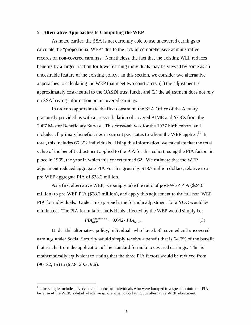
pre-WEP aggregate PIA of $38.3 million.

As a first alternative WEP, we simply take the ratio of post-WEP PIA ($24.6

million) to pre-WEP PIA ($38.3 million), and apply this adjustment to the full non-WEP

PIA for individuals. Under this approach, the formula adjustment for a YOC would be

eliminated. The PIA formula for individuals affected by the WEP would simply be:

WEPNoeAlternativ

WEP PIAPIA ⋅= 642.01 (3)

Under this alternative policy, individuals who have both covered and uncovered

earnings under Social Security would simply receive a benefit that is 64.2% of the benefit

that results from the application of the standard formula to covered earnings. This is

mathematically equivalent to stating that the three PIA factors would be reduced from

(90, 32, 15) to (57.8, 20.5, 9.6).

11 The sample includes a very small number of individuals who were bumped to a special minimum PIA because of the WEP, a detail which we ignore when calculating our alternative WEP adjustment.

15

If policymakers wished to maintain the YOC concept, this approach could be

easily adapted to allow the new formula to gradually revert to the non-WEP formula

based on YOCs. Of course, allowing the YOC credits to reduce the WEP adjustment for

individuals with more YOCs requires a larger adjustment to the base formula in order to

keep it cost neutral. By using the AIME x YOC tabs provided by SSA, we approximate

that the modified formula would reduce the multiplication factor to 0.58, and then

increase the benefits by 0.042 for each YOC between 20 and 30, such that:

( )( )( ) WEPNoeAlternativ

WEP PIAYOCPIA ⋅−⋅+= 20,0max,10min042.058.02 (4)

Because we have constrained the WEP adjustments to be (to a close

approximation) cost neutral, there will of course be both winners and losers from any

such reform, relative to the status quo. Specifically, the adjusted WEP approaches have

been designed to increase benefits for individuals with lower covered AIMEs and reduce

them for individuals with higher covered AIMEs. Of course, the “winners” include both

genuine low earners, and high earners with a small fraction of earnings covered by Social

Security. Without access to uncovered earnings data, it is difficult to avoid this outcome.

Importantly, these “winners” may still end up with a lower ratio of benefits to covered

AIME than fully covered individuals with the same lifetime earnings level. For example,

the “low earner” receives a benefit under either adjusted WEP formula that is higher than

the existing benefit, but still lower than the 46% rate that they would have received were

all earnings covered (i.e., under the proportional WEP). This can be seen in figure 6

below:

16

Figure 6: Ratio of Age 62 Benefit to Covered AIME Under Alternative WEP Rules For Low Earner

0.00%

5.00%

10.00%

15.00%

20.00%

25.00%

30.00%

35.00%

40.00%

45.00%

50.00%

0 4 8 12 16 20 24 28 32 36 40 44 48 52 56 60 64 68 72 76 80 84 88 92 96 100

Percentage of Earnings Covered by Social Security

Rat

io o

f Age

62

Ben

efit

to C

over

ed A

IME

Proportional WEP Cov. Earnings Only w/ WEP Revised WEP #1 Revised WEP #2

The “losers” relative to the status quo are high earners who have substantial

covered earnings. Whether or not these “losers” end up with a higher or lower

replacement rate than they would under the proportional WEP depends in part on whether

the YOC adjustment is used or not. As indicated in Figure 7, the alternative WEP that

ignores the YOC adjustment provides a lower benefit than the proportional WEP baseline

for maximum earners with more than 35% of earnings covered. If the alternative WEP

with a YOC adjustment is used, this alternative remains everywhere higher than the

proportional WEP baseline. Stated differently, with the alternative WEP that includes the

YOC adjustment, even the “losers” still receive a windfall, albeit a smaller one than

under the status quo.

17

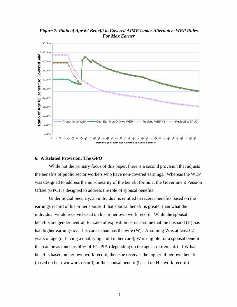
Figure 7: Ratio of Age 62 Benefit to Covered AIME Under Alternative WEP Rules For Max Earner

0.00%

5.00%

10.00%

15.00%

20.00%

25.00%

30.00%

35.00%

40.00%

45.00%

50.00%

0 3 6 9 12 15 18 21 24 27 30 33 36 39 42 45 48 51 54 57 60 63 66 69 72 75 78 81 84 87 90 93 96 99

Percentage of Earnings Covered by Social Security

Rat

io o

f Age

62

Ben

efit

to C

over

ed A

IME

Proportional WEP Cov. Earnings Only w/ WEP Revised WEP #1 Revised WEP #2

6. A Related Provision: The GPO

While not the primary focus of this paper, there is a second provision that adjusts

the benefits of public sector workers who have non-covered earnings. Whereas the WEP

was designed to address the non-linearity of the benefit formula, the Government Pension

Offset (GPO) is designed to address the role of spousal benefits.

Under Social Security, an individual is entitled to receive benefits based on the

earnings record of his or her spouse if that spousal benefit is greater than what the

individual would receive based on his or her own work record. While the spousal

benefits are gender neutral, for sake of exposition let us assume that the husband (H) has

had higher earnings over his career than has the wife (W). Assuming W is at least 62

years of age (or having a qualifying child in her care), W is eligible for a spousal benefit

that can be as much as 50% of H’s PIA (depending on the age at retirement.) If W has

benefits based on her own work record, then she receives the higher of her own benefit

(based on her own work record) or the spousal benefit (based on H’s work record.)

18

For example, suppose that H has a PIA of $2,000. W would be entitled to a

spousal benefit of $1,000 at her NRA even if she had no earnings during her lifetime. If

W did work, and based on her work record was entitled to a worker benefit based on a

PIA of less than $1,000, then she would still receive the benefit based on the $1,000 PIA.

In this sense, the taxes paid on those earnings result in no marginal increase in her benefit

(until she has earnings that would result in a PIA in excess of $1,000). Put differently,

with the spousal benefit in place, W’s own worker benefit is reduced dollar-for-dollar

until she reaches $1,000.

Now suppose that W is a state employee whose earnings are not covered by

Social Security. For simplicity, let’s assume that the pension she receives from the state

is identical to what Social Security would have paid her, and further suppose that this

amounts to $800 per month. If Social Security ignored the fact that she had uncovered

employment, she would receive her state pension benefit ($800) plus the full $1,000

spousal benefit from Social Security, for a total benefit of $1,800. In comparison, had

this same individual worked in covered employment, she would not have received the

$800, and would have received only the $1,000 spousal benefit.

In short, the design of the spousal benefit rules means that working spouses who

are covered by a government pension and not covered by Social Security would receive a

total benefit that is too generous relative to that received by an otherwise identical couple

in which both spouses are covered by Social Security. The GPO is intended to correct

this problem. Originally established in 1977, the GPO reduced spousal benefits dollar-

for-dollar, as does the spousal benefit for covered working spouses. However,

presumably due to the recognition that many government pensions for non-covered

workers are meant to replace both Social Security and a private sector pension, the GPO

calculation was altered in 1983. Specifically, the new legislation replaced the one-for-

one offset with a two-for-three offset, thus reducing the Social Security spousal benefit

by 2/3 of the amount of the government pension.

Like the WEP, the GPO is viewed as unfair by those affected by it. And like the

WEP, the offset could be calculated more accurately if SSA had access to complete

earnings records that included both covered and uncovered earnings.

19

7. Discussion and Conclusions

The Social Security benefit formula was designed to be non-linear in an attempt

to redistribute benefits from higher earning workers to lower earning workers. It was not

designed this way in order to transfer resources from workers who are full participants in

the system to workers who are only partially covered. Yet the simple application of the

standard benefit formula to partially uncovered workers would have exactly this effect.

As such, some form of benefit adjustment for workers with uncovered earnings is clearly

warranted.

Nonetheless, the WEP has proved quite controversial. While many of the

objections to the WEP appear to be ill-informed about the need for a benefit adjustment

in the presence of a non-linear benefit formula, one well-founded objection is that the

WEP hits lower earners disproportionately hard. Our research suggests that, among

individuals subject to the WEP, those individuals with low lifetime earnings receive a

lower ratio of benefits to covered earnings – and thus receive a lower “return” on their

OASDI contributions – than do individuals with higher lifetime earnings.

If SSA had access to a complete set of uncovered earnings records, the

conceptually simple way to make such an adjustment would be to calculate an

individual’s benefit using total (covered plus uncovered) earnings, and then multiply this

by the ratio of covered-to-total lifetime earnings. The SSA, however, does not have

access to reliable earnings histories prior to the early 1980s. In the absence of these data,

it is quite difficult to construct an alternative WEP that maintains the intended degree of

redistribution in Social Security.

Nonetheless, it is possible to construct alternative approaches to the WEP that

come closer to preserving the degree of progressivity in the benefit formula, rely only on

covered earnings data, and are budget neutral.

Short of changing the benefit formula, we speculate that SSA may be able to

reduce some of the public anger towards the existing WEP if its rationale were presented

more clearly, and if it were framed differently. For example, the second sentence in the

online retirement planner on the SSA website (http://www.ssa.gov/retire2/wep-chart.htm)

reads “the following chart shows the maximum monthly amount your benefit can be

reduced because of WEP if you have fewer than 30 years of substantial earnings.” This

20

page provides links to other pages, such as the “Electronic Fact Sheet: Windfall

Elimination Provision” (http://www.ssa.gov/pubs/10045.html), which is the electronic

version of the print publication on the WEP. The first heading is “Your Social Security

retirement or disability benefits may be reduced.” In essence, all the material provided

by SSA frames the WEP as a “benefit reduction.” The same is true with the GPO. The

bold face headings in the official SSA publication that explain the GPO include “how

much will my Social Security benefits be reduced?”

While no direct research on this question has been done (to the knowledge of the

authors), this framing would appear to maximize the probability that participants view

this provision as a “loss.” Alternative framing of the same information might be able to

mitigate some of the anger that the WEP generates. For instance, the information could

discuss “Getting your benefit right” instead of “your benefit may be reduced.” Changes

in how information is framed have been shown in a variety of contexts to influence both

attitudes and behaviors.

The non-monotonic pattern of benefits that are introduced by the YOC adjustment

to the WEP provide interesting labor supply incentives to those who expect to find

themselves in the 20 – 30 YOC range near retirement. Because these marginal incentives

are quite large, future research may be able to use them as a source of variation for

studying how labor supply is affected by Social Security accruals, holding constant total

lifetime earnings.

21

References

Coronado, Julia Lynn, Don Fullerton, and Thomas Glass. 2000. “The Progressivity of Social Security.” NBER Working Paper #7520.

Diamond, Peter A. and Peter Orszag R. 2003. “Reforming the GPO and WEP in Social Security.” Tax Notes. November 3, 2003. pp. 647 – 649.

Gustman, Alan L. and Thomas L. Steinmeier. 2001. “How Effective is Redistribution Under the Social Security Benefit Formula?” The Journal of Public Economics 82.

Liebman, Jeffrey B. 2002. “Redistribution in the Current U.S. Social Security System.” M. Feldstein and J. Liebman, eds., The Distributional Effects of Social Security Reform. Chicago: The University of Chicago Press for NBER.

Social Security Administration. 2005. “Testimony of Frederick Streckewald, Assistant Deputy Commissioner, Disability and Income Security Programs.” Hearing Before the House Ways and Means Subcommittee on Social Security. June 9, 2005. Available at http://www.ssa.gov/legislation/testimony_060905.html.

U.S. General Accounting Office. 2004. “Social Security: Distribution of Benefits and Taxes Relative to Earnings Level.” GAO-04-747.

United States Government Accountability Office. “Social Security: Issues Relating to Noncoverage of Public Employees.” Testimony before the Subcommitee on Social Security, Committee on Ways and Means, House of Representatives. Statement of Barbara D. Bovbjerg. GAO-03-710T. May 1, 2003.

United States Government Accountability Office. “Social Security: Issues Regarding the Coverage of Public Employees.” Testimony before the Subcommitee on Social Security, Pensions, and Family Policy, Committee on Finance, U.S. Senate. Statement of Barbara D. Bovbjerg. GAO-08-248T. November 6, 2007.

22