Please cite this paper as:

Flues, F. and A. Thomas (2015), “The distributional effects ofenergy taxes”, OECD Taxation Working Papers, No. 23,OECD Publishing, Paris.http://dx.doi.org/10.1787/5js1qwkqqrbv-en

OECD Taxation Working Papers No. 23

The distributional effects ofenergy taxes

Florens Flues, Alastair Thomas

JEL Classification: H23, Q40, Q52

1

OECD CENTRE FOR TAX POLICY AND ADMINISTRATION

OECD TAXATION WORKING PAPERS SERIES

This series is designed to make available to a wider readership selected studies drawing on the work of

the OECD Centre for Tax Policy and Administration. Authorship is usually collective, but principal writers

are named. The papers are generally available only in their original language (English or French) with a short

summary available in the other.

OECD Working Papers should not be reported as representing the official views of the OECD or of its

member countries. The opinions expressed and arguments employed are those of the author(s).

Working Papers describe preliminary results or research in progress by the author(s) and are published

to stimulate discussion on a broad range of issues on which the OECD works. Comments on Working Papers

are welcomed, and may be sent to the Centre for Tax Policy and Administration, OECD, 2 rue André-Pascal,

75775 Paris Cedex 16, France. This working paper has been authorised for release by the Director of the

Centre for Tax Policy and Administration, Pascal Saint-Amans.

Comments on the series are welcome, and should be sent to either ctp.contact@oecd.org or the Centre

for Tax Policy and Administration, 2, rue André Pascal, 75775 PARIS CEDEX 16, France.

Applications for permission to reproduce or translate all, or part of, this material should be sent to

OECD Publishing, rights@oecd.org or by fax 33 1 45 24 99 30.

Copyright OECD 2015

2

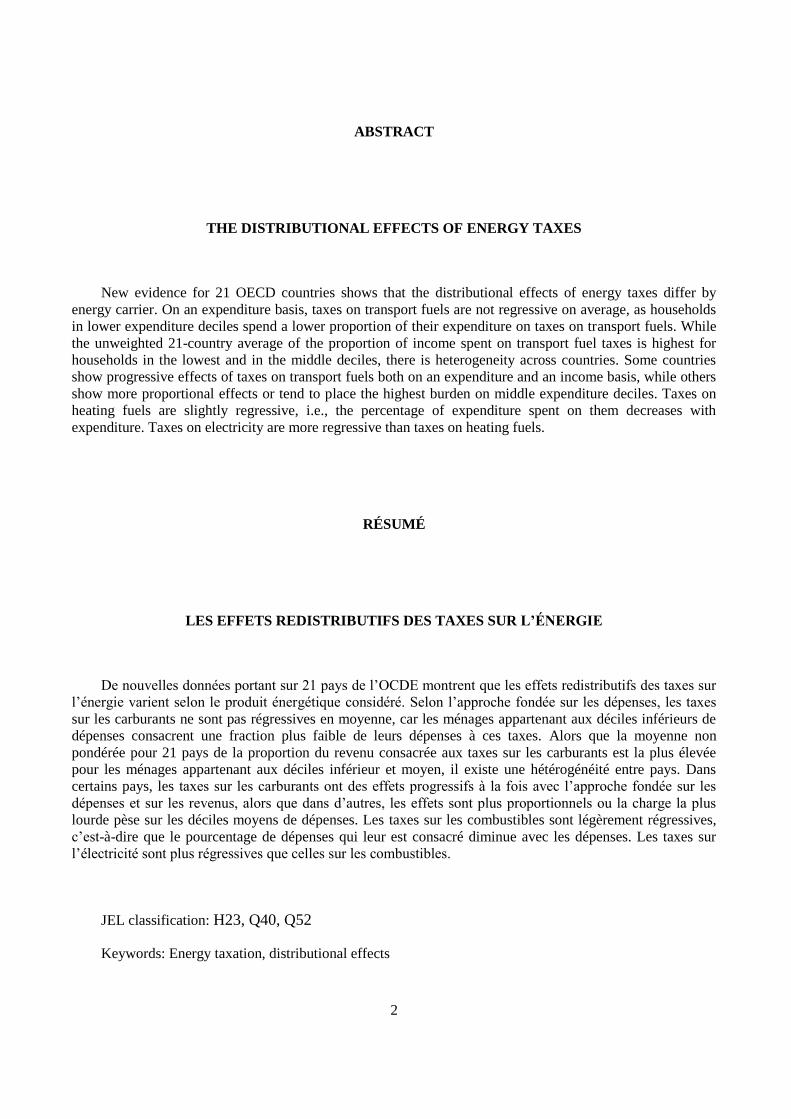
ABSTRACT

THE DISTRIBUTIONAL EFFECTS OF ENERGY TAXES

New evidence for 21 OECD countries shows that the distributional effects of energy taxes differ by

energy carrier. On an expenditure basis, taxes on transport fuels are not regressive on average, as households

in lower expenditure deciles spend a lower proportion of their expenditure on taxes on transport fuels. While

the unweighted 21-country average of the proportion of income spent on transport fuel taxes is highest for

households in the lowest and in the middle deciles, there is heterogeneity across countries. Some countries

show progressive effects of taxes on transport fuels both on an expenditure and an income basis, while others

show more proportional effects or tend to place the highest burden on middle expenditure deciles. Taxes on

heating fuels are slightly regressive, i.e., the percentage of expenditure spent on them decreases with

expenditure. Taxes on electricity are more regressive than taxes on heating fuels.

RÉSUMÉ

LES EFFETS REDISTRIBUTIFS DES TAXES SUR L’ÉNERGIE

De nouvelles données portant sur 21 pays de l’OCDE montrent que les effets redistributifs des taxes sur

l’énergie varient selon le produit énergétique considéré. Selon l’approche fondée sur les dépenses, les taxes

sur les carburants ne sont pas régressives en moyenne, car les ménages appartenant aux déciles inférieurs de

dépenses consacrent une fraction plus faible de leurs dépenses à ces taxes. Alors que la moyenne non

pondérée pour 21 pays de la proportion du revenu consacrée aux taxes sur les carburants est la plus élevée

pour les ménages appartenant aux déciles inférieur et moyen, il existe une hétérogénéité entre pays. Dans

certains pays, les taxes sur les carburants ont des effets progressifs à la fois avec l’approche fondée sur les

dépenses et sur les revenus, alors que dans d’autres, les effets sont plus proportionnels ou la charge la plus

lourde pèse sur les déciles moyens de dépenses. Les taxes sur les combustibles sont légèrement régressives,

c’est-à-dire que le pourcentage de dépenses qui leur est consacré diminue avec les dépenses. Les taxes sur

l’électricité sont plus régressives que celles sur les combustibles.

JEL classification: H23, Q40, Q52

Keywords: Energy taxation, distributional effects

3

FOREWORD

This paper has been written by Florens Flues and Alastair Thomas, and has benefited from comments and

suggestions provided by Bert Brys, David Bradbury, Nils Axel Braathen, James Greene, Michelle Harding,

Herwig Immervoll, Stefano Scarpetta and Kurt van Dender. The paper is part of the broader OECD projects

examining the political economy of environmentally related taxes and the distributional effects of

consumption taxes. Thanks are due to the National Statistical Offices of the following countries for the

provision of, and assistance with, household budget survey micro-data: Austria, Belgium, Chile, the Czech

Republic, Estonia, Finland, France, Germany, Greece, Hungary, Ireland, Italy, Luxembourg, the Netherlands,

Poland, the Slovak Republic, Slovenia, Spain, Switzerland, Turkey and the United Kingdom.

4

TABLE OF CONTENTS

ABSTRACT .................................................................................................................................................... 2

FOREWORD ................................................................................................................................................... 3

EXECUTIVE SUMMARY ............................................................................................................................. 6

RÉSUMÉ ......................................................................................................................................................... 7

1. Introduction .............................................................................................................................................. 8 2. Earlier work on the distributional effects of energy taxes ....................................................................... 9 3. Methodology .......................................................................................................................................... 10

Data ................................................................................................................................................... 10 Calculation of taxes .......................................................................................................................... 11 Assumptions and limitations............................................................................................................. 12 Income versus expenditure ............................................................................................................... 15

4. Distributional effects of taxes on transport fuels, heating fuels and electricity across income and

expenditure deciles ........................................................................................................................... 18 Distributional effects of taxes on transport fuels .............................................................................. 18 Distributional effects of taxes on heating fuels ................................................................................ 25 Distributional effects of taxes on electricity ..................................................................................... 29

5. Distributional effects of energy taxes across socio-demographic factors .............................................. 32 Household type ................................................................................................................................. 33 Population density ............................................................................................................................ 34 Age of household head ..................................................................................................................... 36 Activity of household head ............................................................................................................... 37 Education of household head ............................................................................................................ 39

6. Conclusion and outlook ......................................................................................................................... 40

REFERENCES .............................................................................................................................................. 41

ANNEX I ....................................................................................................................................................... 44

ANNEX I ....................................................................................................................................................... 45

ANNEX II ..................................................................................................................................................... 50

ANNEX III .................................................................................................................................................... 63

5

Tables

Table 1. Share of self-employed, retirees, and other inactive people in total population ............... 16 Table 2. Ratio of households not using a motor vehicle to households using a motor vehicle ....... 20 Table 3. Average transport fuel taxes as % of net income .............................................................. 21 Table 4. Average transport fuel taxes as % of pre-tax expenditure ................................................. 22 Table 5. Average heating fuel taxes as % of net income ................................................................. 27 Table 6. Average heating fuel taxes as % of pre-tax expenditure ................................................... 28 Table 7. Ratio of taxed to untaxed heating fuels across expenditure .............................................. 29 Table 8. Average electricity taxes as % of net income .................................................................... 31 Table 9. Average electricity taxes as % of pre-tax expenditure ...................................................... 32 Table 10. Ratio of taxed to untaxed heating fuels by population density ......................................... 36 Table 11-24. Average energy tax burdens by country and socio-demographics .................................... 45 Table 25-29. Average energy tax burdens by country, expenditure deciles and socio-demographics ... 50

Figures

Figure 1. Average taxes on energy carriers as % of net income or pre-tax expenditure .................... 8 Figure 2. Average transport fuel taxes as % of net income or pre-tax expenditure .......................... 19 Figure 3. Harmonised interquintile range of transport fuel tax burden and GDP per capita ............ 23 Figure 4. Average petrol taxes as % of net income and pre-tax expenditure ................................... 25 Figure 5. Average diesel taxes as % of net income and pre-tax expenditure ................................... 25 Figure 6. Average heating fuel taxes as % of net income or pre-tax expenditure ............................ 26 Figure 7. Average electricity taxes as % of net income or pre-tax expenditure ............................... 30 Figure 8. Average transport fuel taxes as % of pre-tax expenditure across household type ............ 33 Figure 9. Average heating fuel taxes as % of pre-tax expenditure across household type ............... 33 Figure 10. Average electricity taxes as % of pre-tax expenditure across household type .................. 34 Figure 11. Average transport fuel taxes as % of pre-tax expenditure across population density........ 34 Figure 12. Average heating fuel taxes as % of pre-tax expenditure across population density .......... 35 Figure 13. Average electricity taxes as % of pre-tax expenditure across population density ............. 35 Figure 14. Average transport fuel taxes as % of pre-tax expenditure across age ................................ 36 Figure 15. Average heating fuel taxes as % of pre-tax expenditure across age .................................. 37 Figure 16. Average electricity taxes as % of pre-tax expenditure across age ..................................... 37 Figure 17. Average transport fuel taxes as % of pre-tax expenditure across activity status ............... 38 Figure 18. Average heating fuel taxes as % of pre-tax expenditure across activity status ................. 38 Figure 19. Average electricity taxes as % of pre-tax expenditure across activity status .................... 38 Figure 20. Average transport fuel taxes as % of pre-tax expenditure across education level ............. 39 Figure 21. Average heating fuel taxes as % of pre-tax expenditure across education level ............... 39 Figure 22. Average electricity taxes as % of pre-tax expenditure across education level .................. 40 Figure 23. Average taxes on energy carriers as % of pre-tax expenditure by country ....................... 64

6

THE DISTRIBUTIONAL EFFECTS OF ENERGY TAXES

EXECUTIVE SUMMARY

A major obstacle to the more widespread use of energy taxation is the concern that energy taxes may be

regressive, hitting the poor harder than the rich. Evidence is surprisingly scarce with only a few studies

investigating the distributional effects of energy taxes in OECD countries. This paper adds to this evidence by

providing a systematic analysis of the distributional effects of the main energy taxes in 21 OECD countries.

The distributional effects of taxes can be assessed using an income or expenditure basis. Although there

are arguments for using either, households with low transitory income, who are not poor across their lifetime,

strongly affect average income while they have less of an effect on average expenditure. The analysis in this

paper emphasises the expenditure-based analysis but shows income-based results too, recognising that the

choice of basis affects results and interpretations.

New evidence for 21 OECD countries shows that the distributional effects of energy taxes differ by

energy carrier. On an expenditure basis, taxes on transport fuels are not regressive on average, as households

in lower expenditure deciles spend a lower proportion of their expenditure on taxes on transport fuels. While

the unweighted 21-country average of the proportion of income spent on transport fuel taxes is highest for

households in the lowest and in the middle deciles, there is heterogeneity across countries. Some countries

show progressive effects of taxes on transport fuels both on an expenditure and an income basis, while others

show more proportional effects or tend to place the highest burden on middle expenditure deciles. Taxes on

heating fuels are slightly regressive, i.e., the percentage of expenditure spent on them decreases with

expenditure. Taxes on electricity are more regressive than taxes on heating fuels.

Socio-demographic characteristics influence the distributional effects of energy taxes. Larger households

spend a higher share of their expenditure on energy taxes than smaller ones, especially on taxes on transport

fuels. Households in rural areas spend, on average, more of their expenditure on energy taxes than households

in urban areas. If the household head is above 60 years of age, households tend to spend a smaller share of

their expenditure on taxes on transport fuels.

The average distributional outcomes are calculated over the set of 21 OECD countries and as such

should not be taken to reflect OECD-wide average patterns. Some of the countries that are not included

differ from the countries studied in terms of socio-demographic characteristics, including those that affect

distributional outcomes.

7

LES EFFETS REDISTRIBUTIFS DES TAXES SUR L’ÉNERGIE

RÉSUMÉ

La crainte que les taxes sur l’énergie puissent avoir un effet régressif et ainsi pénaliser davantage les

pauvres que les riches constitue un obstacle de taille à une utilisation plus fréquente de ces taxes. Les travaux

de recherche sur ce sujet sont étonnamment peu nombreux, et quelques études seulement examinent les effets

redistributifs des taxes sur l’énergie dans les pays de l’OCDE. Ce rapport vient enrichir les données

disponibles en menant une analyse systématique des effets redistributifs des principales taxes sur l’énergie

appliquées dans 21 pays de l’OCDE.

On peut évaluer les effets redistributifs des taxes selon une approche fondée sur les revenus ou sur les

dépenses. Bien qu’il existe des arguments en faveur de l’utilisation de l’une ou l’autre de ces méthodes, les

ménages disposant d’un revenu transitoire faible, qui ne sont pas dans une situation de pauvreté tout au long

de leur vie, exercent une forte influence sur le revenu moyen mais influent beaucoup moins sur les dépenses

moyennes. Ce document met l’accent sur l’analyse fondée sur les dépenses, mais indique également les

résultats d’une analyse basée sur les revenus, en reconnaissant que le choix de l’approche influe sur les

résultats et sur les interprétations.

De nouvelles données portant sur 21 pays de l’OCDE montrent que les effets redistributifs des taxes sur

l’énergie varient selon le produit énergétique considéré. Selon l’approche fondée sur les dépenses, les taxes

sur les carburants ne sont pas régressives en moyenne, car les ménages appartenant aux déciles inférieurs de

dépenses consacrent une fraction plus faible de leurs dépenses à ces taxes. Alors que la moyenne non

pondérée pour 21 pays de la proportion du revenu consacrée aux taxes sur les carburants est la plus élevée

pour les ménages appartenant aux déciles inférieur et moyen, il existe une hétérogénéité entre pays. Dans

certains pays, les taxes sur les carburants ont des effets progressifs à la fois avec l’approche fondée sur les

dépenses et sur les revenus, alors que dans d’autres, les effets sont plus proportionnels ou la charge la plus

lourde pèse sur les déciles moyens de dépenses. Les taxes sur les combustibles sont légèrement régressives,

c’est-à-dire que le pourcentage de dépenses qui leur est consacré diminue avec les dépenses. Les taxes sur

l’électricité sont plus régressives que celles sur les combustibles.

Les caractéristiques socioéconomiques influent sur les effets redistributifs des taxes sur l’énergie. Les

ménages de grande taille consacrent une fraction plus élevée de leurs dépenses aux taxes énergétiques que les

ménages de petite taille, notamment aux taxes sur les carburants. En moyenne, les ménages en milieu rural y

consacrent un pourcentage de leurs dépenses plus élevé que les ménages vivant en zone urbaine. Si le chef de

famille est âgé de plus de 60 ans, les taxes sur les carburants absorbent généralement une part plus faible des

dépenses du ménage.

Les effets redistributifs moyens sont calculés sur un ensemble de vingt-et-un pays de l'OCDE. Ces

résultats ne sont pas représentatifs en tant que tels des tendances moyennes pour l’ensemble de l’OCDE.

Certains des pays qui ne sont pas inclus diffèrent des pays étudiés en ce qui concerne leurs caractéristiques

sociodémographiques. Ces dernières peuvent aussi avoir une influence sur les effets redistributifs.

8

1. Introduction

1. It is often claimed that excise taxes on energy, henceforth referred to as energy taxes, are regressive,

i.e. that poorer households spend a higher share of their income on energy taxes than richer households. This

leads to concerns that lower income households, and in particular the poor, would be hit particularly hard by

higher energy taxes. This perception makes it harder to implement or increase such taxes.

2. This paper examines the actual distributional effects of energy taxes for 21 OECD countries. The

analysis is based on an energy tax micro-simulation model constructed using household expenditure micro-

data, i.e. expenditure measured at the household level. It builds upon and complements recent OECD work

examining the distributional effects of value-added taxes and selected other consumption taxes (OECD,

2014a). The household level expenditure data is used to model energy tax burdens across the income and

expenditure distributions. The micro-simulations assess whether total energy taxes and individual taxes on

transport fuels, heating fuels and electricity are proportional, progressive or regressive. When examined

across the income or expenditure distribution, “progressive” means that households in lower income or

expenditure deciles spend a lower share of income or expenditure on energy taxes, “regressive” means the

share decreases as income or expenditure increases and “proportional” indicates the share does not depend on

income or expenditure.

3. The distributional effects of energy taxes can be assessed by measuring tax burdens as a percentage

of income across the income distribution and as a percentage of expenditure across the expenditure

distribution. Although there are arguments for using either measure as discussed in Section 3, a key issue is

that households with low transitory income, who are not lifetime poor, strongly affect average income while

they do not affect average expenditure as much. The analysis in this paper emphasises the analysis on an

expenditure basis1 but shows income-based results too.

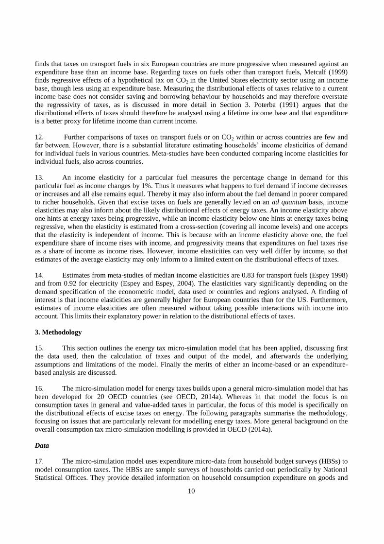
4. The unweighted country average for the 21 countries analysed shows that the distributional effects

differ across taxes on transport fuels, heating fuels, and electricity, see Figure 1. Taxes on transport fuels are

roughly proportional on an income basis and tend to be progressive on an expenditure basis. Taxes on heating

fuels are slightly regressive, and taxes on electricity are more regressive on both an income and expenditure

basis.

Figure 1. Average taxes on energy carriers as % of net income or pre-tax expenditure (21-country averages)

1 . The paper provides results both as a percentage of income across income deciles and as a percentage of

expenditure across expenditure deciles. In the following the formulation “income basis” refers to any comparison

across income, tax burdens measured as a percentage of income and a combination of both of them. The

formulation “income base” refers only to tax burdens measured as a percentage of income, i.e., the tax base. The

same terminology applies to “expenditure basis” and “expenditure base”.

0.0%

0.5%

1.0%

1.5%

2.0%

1 2 3 4 5 6 7 8 9 10

% o

f n

et

inco

me

Income Deciles

Transport Fuels Heating Fuels Electricity

0.0%

0.5%

1.0%

1.5%

2.0%

1 2 3 4 5 6 7 8 9 10

% o

f p

re-t

ax e

xpe

nd

itu

re

Expenditure Deciles

Transport Fuels Heating Fuels Electricity

9

5. Across socio-demographic factors three patterns emerge in the 21 countries analysed. First, larger

households spend a higher share of their income and expenditure on energy taxes than smaller ones,

particularly on transport fuel taxes. Second, households in rural areas spend on average more of their income

and expenditure on all energy taxes than households in urban areas. Third, households tend to spend less of

their income and expenditure on taxes on transport fuels if the household head is above 60 years of age.

6. The average distributional outcomes are calculated over the set of 21 OECD countries and as such

should not be taken to reflect OECD-wide patterns. Some of the countries that are not included differ from

the countries studied in terms of socio-demographic characteristics, including those that affect distributional

outcomes. The study examines the distributional effects of current energy tax settings and as such does not

model any behavioural responses to potential energy tax reforms.

7. This paper proceeds as follows: Section 2 discusses earlier work on the distributional analysis of

energy taxes. Section 3 details the methodology of the micro-simulation model, its assumptions, and the data

on which it is based. It also discusses the merits and drawbacks of using expenditure or income as the basis

for the distributional analysis. Section 4 presents the core results. It looks at the distributional effects of

energy taxes when separated into different taxes according to energy use, i.e., on taxes on transport fuels,

heating fuels, and electricity. Section 5 analyses the relationship between energy taxes and demographic

characteristics. Section 6 concludes and makes suggestions for future work.

2. Earlier work on the distributional effects of energy taxes

8. This paper extends earlier work on the distributional effects of energy taxes in two ways. First, it

analyses energy taxes within a homogenous framework across countries. Second, it analyses taxes across

different energy carriers and usage, i.e., taxes on transport fuels, heating fuels and electricity within a

homogenous framework. So far, cross-country comparisons on the distributional effects of energy taxes have

focused on particular fuels. Comparisons of taxes on different fuels have, to our knowledge, not been made.

However, there is a substantial literature estimating households’ income elasticities of demand for individual

fuels in various countries, which can give some insight into the distributional effects of energy taxes across

countries. In the following, studies that analyse explicitly the distributional effects of energy taxes will be

discussed first. Second, main results from studies comparing income elasticities of energy demand are

provided.

9. Studies on the distributional effects of transport fuels find, first, that the effects differ across

countries. Some countries show regressive effects, other countries proportional or even progressive effects.

Second, taxes on transport fuels are more progressive when measured against an expenditure base than an

income base.

10. Comparing the distributional effects of taxes on transport fuels for France, Germany, Italy, Serbia,

Spain, Sweden and the United Kingdom, Sterner (2012) finds slight regressivity using an income base for

half of the countries. Serbia shows clearly progressive effects of taxes on transport fuels while in Germany

and the United Kingdom, households in middle income deciles spend less of their income on transport fuels

than households in lower and higher income deciles. Sterner hypothesises that the difference in the

distributional effects of taxes on transport fuels across countries is due to different usage of cars by different

income groups and the availability of public transport. Poorer households may be less likely to own a car,

especially in poorer countries, making taxes on transport fuels progressive. Lack of public transport may,

however, lead to regressive effects of taxes on transport fuels.

11. Analysing taxes on transport fuels in the United States, Poterba (1991) and Metcalf (1999) find that

taxes on transport fuels are regressive when measured as a percentage of current income across income

deciles. However, when measured against an expenditure or life-time income base, taxes on transport fuels

look more progressive and tend to put the highest burden on middle expenditure deciles. Sterner (2012) also

10

finds that taxes on transport fuels in six European countries are more progressive when measured against an

expenditure base than an income base. Regarding taxes on fuels other than transport fuels, Metcalf (1999)

finds regressive effects of a hypothetical tax on CO2 in the United States electricity sector using an income

base, though less using an expenditure base. Measuring the distributional effects of taxes relative to a current

income base does not consider saving and borrowing behaviour by households and may therefore overstate

the regressivity of taxes, as is discussed in more detail in Section 3. Poterba (1991) argues that the

distributional effects of taxes should therefore be analysed using a lifetime income base and that expenditure

is a better proxy for lifetime income than current income.

12. Further comparisons of taxes on transport fuels or on CO2 within or across countries are few and

far between. However, there is a substantial literature estimating households’ income elasticities of demand

for individual fuels in various countries. Meta-studies have been conducted comparing income elasticities for

individual fuels, also across countries.

13. An income elasticity for a particular fuel measures the percentage change in demand for this

particular fuel as income changes by 1%. Thus it measures what happens to fuel demand if income decreases

or increases and all else remains equal. Thereby it may also inform about the fuel demand in poorer compared

to richer households. Given that excise taxes on fuels are generally levied on an ad quantum basis, income

elasticities may also inform about the likely distributional effects of energy taxes. An income elasticity above

one hints at energy taxes being progressive, while an income elasticity below one hints at energy taxes being

regressive, when the elasticity is estimated from a cross-section (covering all income levels) and one accepts

that the elasticity is independent of income. This is because with an income elasticity above one, the fuel

expenditure share of income rises with income, and progressivity means that expenditures on fuel taxes rise

as a share of income as income rises. However, income elasticities can very well differ by income, so that

estimates of the average elasticity may only inform to a limited extent on the distributional effects of taxes.

14. Estimates from meta-studies of median income elasticities are 0.83 for transport fuels (Espey 1998)

and from 0.92 for electricity (Espey and Espey, 2004). The elasticities vary significantly depending on the

demand specification of the econometric model, data used or countries and regions analysed. A finding of

interest is that income elasticities are generally higher for European countries than for the US. Furthermore,

estimates of income elasticities are often measured without taking possible interactions with income into

account. This limits their explanatory power in relation to the distributional effects of taxes.

3. Methodology

15. This section outlines the energy tax micro-simulation model that has been applied, discussing first

the data used, then the calculation of taxes and output of the model, and afterwards the underlying

assumptions and limitations of the model. Finally the merits of either an income-based or an expenditure-

based analysis are discussed.

16. The micro-simulation model for energy taxes builds upon a general micro-simulation model that has

been developed for 20 OECD countries (see OECD, 2014a). Whereas in that model the focus is on

consumption taxes in general and value-added taxes in particular, the focus of this model is specifically on

the distributional effects of excise taxes on energy. The following paragraphs summarise the methodology,

focusing on issues that are particularly relevant for modelling energy taxes. More general background on the

overall consumption tax micro-simulation modelling is provided in OECD (2014a).

Data

17. The micro-simulation model uses expenditure micro-data from household budget surveys (HBSs) to

model consumption taxes. The HBSs are sample surveys of households carried out periodically by National

Statistical Offices. They provide detailed information on household consumption expenditure on goods and

11

services, possession of durable goods and housing. They include demographic and socio-economic

characteristics of the surveyed households, including disposable income. Regarding energy taxes, household

expenditure for the following goods is of interest: transport fuels, heating fuels, and electricity.

18. To enhance consistency across countries, the standardised Eurostat-format HBS micro-data is used.

Micro-data from non-European Union countries is adjusted to approximate the Eurostat-format as closely as

possible. The homogenised format allows a standard model to be developed and applied to each country,

rather than requiring country-specific models. While the micro-data is not generally publicly available, data

was provided specifically for the micro-simulations by the respective national statistical offices.

19. The Eurostat-format HBS micro-data is provided by countries to Eurostat once every five-years.

The data in the most recent data-provision cycle relates to various years from 2008 to 2012.2 The countries

modelled in this paper where data was provided in the Eurostat-format (with year in parenthesis) are: Finland

(2012); France (2011); Belgium, the Czech Republic, Estonia, Greece, Hungary, Luxembourg, Italy3, Poland,

the Slovak Republic, Slovenia, Spain (2010); Austria (2009); Germany (2008); Ireland and the Netherlands

(2004). Data for the latter two countries relates to the previous Eurostat data-provision round. In addition,

non-standardised data has been obtained for Chile (2012), Switzerland (2011)4, Turkey and the United

Kingdom (2010).

Calculation of taxes

20. Three types of taxes are simulated for energy carriers: VAT, ad valorem excise duties, and ad

quantum excise duties. The model is constructed by matching expenditure from the HBS data to its

corresponding tax rates (VAT and excise duties). A micro-simulation programme then calculates the amount

of VAT and excise duties paid by each household by applying the tax rates to the corresponding expenditure

amounts. Where excise duties are levied, the simulation order is: ad quantum excises, then ad valorem

excises, and finally VAT. This is the approach taken by all countries currently covered, and means that each

tax base includes the tax amounts of the previous tax(es).

21. The model calculates tax burdens for individual households, average tax burdens across

equivalised5 net income and equivalised pre-tax expenditure deciles, and the aggregate population. Results

can be broken down by the following demographic characteristics of the household or head of household:

family type, sex, age, economic activity status, education level, population density, and combinations of

these. The number of observations in some of these subgroups may become too small to allow sufficiently

reliable statistical inference, however. The paper therefore only shows results for subgroups with 30 or more

observations.

2. Distributional patterns can change over time. When examining results for countries for which the HBS micro-

data dates back several years the reader should bear this in mind. In particular forecasts based on such data may

be inaccurate.

3. Note that the data for Italy does not include an income variable which limits some of the analysis that can be

undertaken for the country.

4. Note that the data for Switzerland is derived from three separate surveys for 2009, 2010 and 2011.

5. The “OECD-modified” scale for “equivalised” income provides a weight of 1 for the first adult household

member, 0.5 for the second and each additional household member aged 14 and over, and 0.3 for each child

under 14. Pre-tax income is divided by the total family weight to determine the family’s “equivalised” income.

The same procedure is applied to expenditure to calculate “equivalised” expenditure.

12

Assumptions and limitations

22. The micro-simulation modelling and resulting analysis have several limitations. These are discussed

below.

Income data

23. Results based on HBS income data at low income levels may be misleading due to the presence of

households with transitorily low income (Bozio et al., 2012; Decoster et al., 2010).6 For example, many self-

employed workers may have low income levels at certain stages of their businesses’ development, but will

continue to have unaltered expenditures. Alternatively, some households may be drawing down savings to

fund their consumption. Also students can have consumption patterns that more accurately reflect their

expected lifetime annual earnings than their incomes while they are studying. In either case, it is likely to be

misleading to consider them “low-income” households for distributional analysis.

24. To mitigate this concern, households are excluded from the analysis where:

the household reports negative or zero income; and

the household has an expenditure-to-income ratio of four or greater.

Tax incidence

25. The modelling attributes the entire consumption tax incidence to the final consumer. This is a

standard assumption made in most consumption tax studies (see, e.g. IFS, 2011; Leahy, Lyons and Tol, 2011;

Decoster et al., 2010). However, it should be noted that consumption taxes may in some cases be less than

fully (or even more than fully) passed on to consumers.7

Ad quantum excise duties

26. Many environmentally related taxes, such as energy taxes, are levied in the form of ad quantum

excise duties. Ad quantum excise duties pose a modelling difficulty as data on the quantity consumed is not

generally available in the HBS data. In the absence of quantity data, average prices (generally provided by

National Statistics Offices) for each energy product are used to estimate quantities from the HBS expenditure

data in order to simulate these taxes.8

27. Assuming both average prices and expenditure information are accurate, aggregate tax figures will

also be accurate. However, some inaccuracy may result at the individual level. Specifically, for households

that consume product varieties that are more (or less) expensive than average or pay higher (or lower) prices

6. The reliability of income data is an issue across all income levels. Previous studies (e.g. Decoster et al., 2010)

suggest that income is generally under-reported to at least some extent in household budget surveys. There is also

evidence to suggest that income may be under-reported to a greater extent for some income sources (e.g. self-

employment income) than others (see, for example, Hurst et al., 2013).

7 . IHS (2011) discusses the theoretical and empirical literature on pass-through of VAT and excise taxes. Bushnell

et al. (2013), Fabra and Reguant (2013) and Sijm et al. (2006) estimate cost pass-through of carbon emission

permits in electricity markets.

8.

Monetary expenditure is divided by the average price to obtain an estimate of the quantity purchased. The ad

quantum rate is then applied to this estimated quantity to estimate the tax paid.

13

than the average for the same product, higher (or lower) taxes than they actually pay will be simulated

because it will be assumed that they consume higher (or lower) quantities than they actually do.9

28. Energy carriers are fairly homogenous goods. It is therefore unlikely that households consume

different qualities of natural gas or electricity, but regional price differences may exist. These will cause

inaccuracies in the measurement of tax burdens between households as described above. It is not clear

whether these potential inaccuracies are likely to affect poorer or richer households differently, and thereby

bias results in one or another direction.

29. Prices may also differ based on household characteristics. At least two cases may occur. First, poor

households may be eligible for certain social tariffs in some countries. In this case, poor households would

consume more energy and pay more taxes than estimated by the model. Second, well-off households may

face lower rates as they have better credit-ratings and can thereby choose their energy provider from a wider

range of competitors. In this situation, well-off households would consume more energy and pay higher taxes

than estimated by the model.

Electricity

30. While some countries tax electricity directly, others tax the fuels used for electricity generation or

both the fuels and electricity.10,11,12

In the case where electricity is taxed directly, the discussion above

regarding ad quantum excise duties applies, i.e., the quantity of electricity consumed has to be calculated with

the help of average electricity prices. If the fuels for electricity generation are taxed, the effective electricity

tax rate for households also has to take into account the country’s electricity generation mix. First, the amount

of electricity consumed is calculated based on average prices; second, the underlying fuel consumption is

calculated based on the country’s effective generation mix, which in turn relies on the efficiency of

transforming fuels into energy. Efficiency factors and the generation mix are calculated from the extended

International Energy Agency (IEA, 2014a) World Energy Balances, applying the methodology used in

Taxing Energy Use (OECD, 2013). This approach captures the current tax incidence of direct or indirect taxes

on electricity consumption.

Carbon taxes

31. Carbon taxes are attributed to fuels based on their carbon content. In the case of electricity, the

effective carbon tax rate for households relies therefore both on the country’s generation mix, which

determines the carbon intensity of electricity generation, and on the carbon taxation of fuels that are inputs to

electricity generation.

32. In addition to carbon taxes, average yearly prices of carbon emission permits are mapped into

effective carbon prices on electricity. To calculate the effective carbon price on electricity, average yearly

carbon emission permit prices are multiplied with the average carbon intensity of electricity generation for

each country. For countries participating in the EU Emission Trading Scheme (ETS), data for emission

9. Note that the estimation of price elasticities is seriously challenged when there is unknown price variation

between households within countries as variation that is essential for the identification of price elasticities is

unknown. Identification of tax burdens across households is nevertheless possible, with unknown price variation

between households possibly causing some inaccuracies as described within the subsection.

10. Excise duties on energy are taken from the EUs excise duty tables (European Commission, 2013) where

applicable.

11 . Inputs to electricity production are only taxed in Belgium, Greece, Italy, Turkey and Switzerland.

12 . Levies to finance feed-in tariffs are not modelled.

14

permit prices are obtained from the European Environment Agency (EEA, 2011) and data on the carbon

intensity from the IEA (2014b).13

Heating fuels

33. Natural gas14

, heating oil and solid fossil fuels for heating purposes in households are taxed in most

of the countries analysed. For both natural gas and heating oil the general discussion regarding ad quantum

excise duties applies, i.e., the quantity of electricity consumed is calculated with the help of average

electricity prices.

34. For solid fuels there is only one variable in the HBS micro-data. This variable contains both solid

fossil fuels and renewable solid fuels, e.g., wood. Solid fossil fuels are generally taxed while renewable solid

fuels are not taxed in the countries analysed. Therefore total solid heating fuel consumption is first separated

into fossil solid fuel and renewable solid fuel consumption using aggregate solid fuel consumption data for

households by country from the extended IEA World Energy Balances of the International Energy Agency

(IEA, 2014a). Second, quantities of solid fossil fuels are calculated using price data on solid fossil fuels as

provided by national statistical offices. If households consume different solid fuels, an average price on solid

fossil fuels is calculated according to share of each fossil solid fuel in overall fossil solid fuel consumption by

households, again using data from the extended IEA World Energy Balances (IEA, 2014a). Third, taxes on

solid fossil fuels are calculated based on the derived consumption of solid fossil fuels. For countries where

less than 10% of all solid fuel consumption is from fossil fuels it has been assumed that no solid fuels are

taxed.

35. There are no excise taxes on district heating consumption in the countries analysed. Hence no taxes

on district heating consumption are modelled. Finland taxes the inputs to district heating and provided an

effective tax rate based on the taxation of the inputs to district heating to the Secretariat, which is taken into

account. For those Finnish households that pay for district heating via the maintenance costs of their dwelling

the district heating burden is calculated based on information of maintenance fees by income decile.

Transport fuels

36. For most countries, the HBS micro-data has only one variable for transport fuels. In order to

simulate excise duties on petrol and diesel, additional information is needed to apportion total expenditures

on transport fuels between petrol and diesel. This task is further complicated by the fact that relative

expenditure on petrol and diesel vary across the income distribution. We follow four different approaches due

to the differing levels of information available across countries.

37. First, for Chile, Switzerland and the United Kingdom a separate variable is available for both petrol

and diesel in the HBS data. As such, no apportionment is necessary.

38. Second, for Austria and Belgium additional data was obtained from national statistical offices. For

Austria, decile averages for petrol and diesel expenditure were provided by the Austrian Statistical Agency,

calculated from the separate petrol and diesel variables in the non-standardised version of the Austrian HBS

data. These averages are used to apportion the single transport fuels variable in the standardised HBS data.

13. This approach follows from taking taxes on energy inputs as indirect taxes on electricity consumption into

account. It assumes that the opportunity costs of carbon emission permits are passed through to households.

Findings from Bushnell et al. (2013) support that electricity producers under EU ETS were able to pass-through

the opportunity costs of carbon emission permits into electricity prices.

14. Taxes on propane-butane gases for cooking purposes have not been modelled as they are only used in a few

countries by few households. Furthermore average price data is hardly available for propane-butane gases.

15

For Belgium the same procedure is followed except that apportionment is based on quartile averages of petrol

and diesel consumption, which are publicly available from the Belgian Statistical Office.

39. Third, for Germany, the Netherlands and France apportionment is based on estimates of the average

expenditure on petrol and diesel consumed by different income bands (Germany), income deciles

(Netherlands) or expenditure deciles (France). These estimates are based on national transport survey data

(Bundesministerium für Verkehr, Bau und Stadtentwicklung, 2010; and Ministerie van Verkeer en

Waterstaat, 2005; SOeS - Inrets – Insee, 2008) that provide information on the average distance driven by

petrol and diesel vehicles across fixed income bands, income deciles or expenditure deciles. These averages

are then multiplied by average fuel efficiency rates (Destatis, 2010; Verbruiksmonitor, 2014; Inspection

générale des finances and Conseil général de l’économie, de l’industrie, de l’énergie et des technologies,

2012) and average price figures (European Commission, 2011) to estimate the average expenditure on petrol

and diesel across income bands, income deciles or expenditure deciles. Note that the same data is also

available for the United Kingdom (Department for Transport, 2011, Department for Transport, 2013 and

European Commission, 2011), and is utilised as described in footnote 15.15

40. Fourth, for all remaining countries, apportionment is based on the overall stock of petrol and diesel

cars in each country (obtained from Eurostat, 2012, 2013). However, these figures are adjusted to account for

the variation in petrol-to-diesel consumption across income quintiles based on the average variation shown in

the more detailed data available for Austria, Germany, and the United Kingdom.16, 17

Income versus expenditure

41. A key issue encountered when working with expenditure micro-data to examine the distributional

effects of consumption taxes is how to present results. Both income and expenditure can be used to measure

the magnitude of tax burdens and to distinguish between poor and rich households.

15. The calculation of kilometres travelled by petrol and diesel vehicles by household’ incomes for the Netherlands

was undertaken by the Secretariat given that the national travel survey micro-data is available free of charge for

research purposes. For Germany and the United Kingdom, information on the kilometres travelled by petrol and

diesel vehicles by household’ incomes was obtained through personal communication with country experts from

the Centre for European Economic Research (ZEW), Mannheim and from the Imperial College, London.

16 . To separate total expenditures on transport fuels into separate expenditures on petrol and diesel by households’

incomes three steps are undertaken. First, average ratios by income quintile of the ratio of petrol to diesel

expenditures by income quintile to the overall ratio of petrol to diesel expenditures are calculated for Austria,

Germany and the United Kingdom. These average ratios, ordered from the lowest income quintile to the highest

income quintile, are 1.6, 1.2, 0.9, 0.8, and 0.6. These average ratios say that a household in the lowest income

quintile is 1.6 times more likely to spend money on petrol than on diesel than the national average, while a

household in the highest income quintile is 0.6 times less likely to do so. Second the three-country averages of

these ratios are multiplied by the country-specific overall ratio of petrol to diesel cars to obtain an imputed ratio

of petrol to diesel expenditure by income quintiles. Third, the imputed ratio of petrol to diesel expenditure by

income quintiles is used to apportion total transport fuel expenditure into separate expenditures on petrol and on

diesel by income quintiles.

17. A comparative analysis of Austria, Germany, the Netherlands and the United Kingdom revealed three stylized

facts on petrol and diesel expenditures. First, across countries, the overall ratio of petrol to diesel expenditures

differs. Second, within countries, the ratio of petrol to diesel expenditures differs by income level – with richer

households tending to spend more on diesel than poorer households. Third, the ratio of the two remains fairly

similar across countries. That is, across all four countries, poorer households tend to spend relatively more on

petrol than the national average, while richer households tend to spend more on diesel than the national average.

16

42. Which measure is preferable depends on the question being asked. If the analyst is interested in

comparing the effects of consumption taxes with taxes that are levied on an income base such as personal

income taxes, then measuring consumption tax burdens as a proportion of current income across income

deciles may be preferable. This allows calculating the total tax burden faced by households as a result of the

entire (income plus consumption) tax system (see, for example, O'Donoghue et al., 2004). It is the

distributional effect of the tax (and benefit) system as a whole that policy makers should be most concerned

with when considering the merits of potential reforms, as opposed to the impact of any one component. Also,

if the interest is to analyse how single compensation schemes may alter the distributional effects of

consumption taxes, measuring consumption tax burdens as a proportion of current income across income

deciles is likely preferable. This is because households are generally compensated on an income, and not on

an expenditure base.

43. Under this approach, however, it is important to also consider what household types fall within each

decile. For example, some self-employed households and retired households in the bottom income decile may

be funding additional expenditure by drawing down savings, while self-employed and students may be

borrowing against future expected income. As such, these households may not necessarily warrant as much

concern from a distributional perspective as other households in the bottom income decile that both earn and

spend little. Despite this, their increased expenditure will make their consumption tax burden appear

particularly high relative to their income, and increase the average tax burden faced by the entire decile.

While such households are still of clear interest to policy makers, from a methodological perspective, the

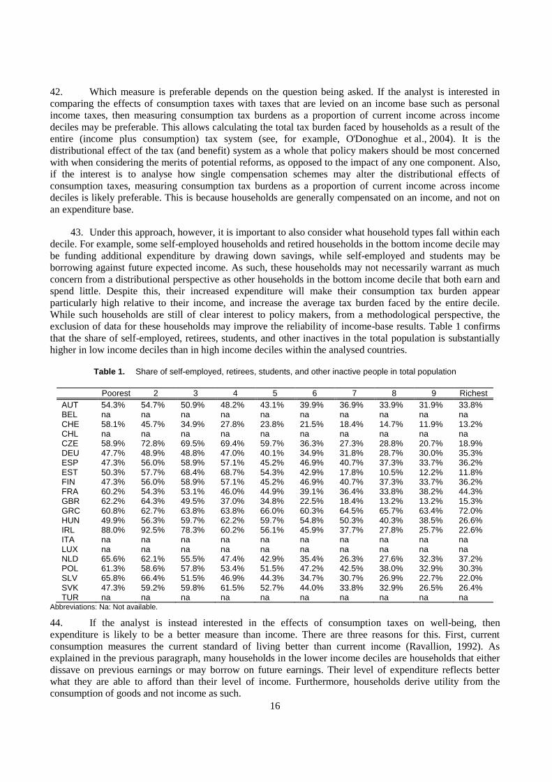
exclusion of data for these households may improve the reliability of income-base results. Table 1 confirms

that the share of self-employed, retirees, students, and other inactives in the total population is substantially

higher in low income deciles than in high income deciles within the analysed countries.

Table 1. Share of self-employed, retirees, students, and other inactive people in total population

Poorest 2 3 4 5 6 7 8 9 Richest

AUT 54.3% 54.7% 50.9% 48.2% 43.1% 39.9% 36.9% 33.9% 31.9% 33.8% BEL na na na na na na na na na na CHE 58.1% 45.7% 34.9% 27.8% 23.8% 21.5% 18.4% 14.7% 11.9% 13.2% CHL na na na na na na na na na na CZE 58.9% 72.8% 69.5% 69.4% 59.7% 36.3% 27.3% 28.8% 20.7% 18.9% DEU 47.7% 48.9% 48.8% 47.0% 40.1% 34.9% 31.8% 28.7% 30.0% 35.3% ESP 47.3% 56.0% 58.9% 57.1% 45.2% 46.9% 40.7% 37.3% 33.7% 36.2% EST 50.3% 57.7% 68.4% 68.7% 54.3% 42.9% 17.8% 10.5% 12.2% 11.8% FIN 47.3% 56.0% 58.9% 57.1% 45.2% 46.9% 40.7% 37.3% 33.7% 36.2% FRA 60.2% 54.3% 53.1% 46.0% 44.9% 39.1% 36.4% 33.8% 38.2% 44.3% GBR 62.2% 64.3% 49.5% 37.0% 34.8% 22.5% 18.4% 13.2% 13.2% 15.3% GRC 60.8% 62.7% 63.8% 63.8% 66.0% 60.3% 64.5% 65.7% 63.4% 72.0% HUN 49.9% 56.3% 59.7% 62.2% 59.7% 54.8% 50.3% 40.3% 38.5% 26.6% IRL 88.0% 92.5% 78.3% 60.2% 56.1% 45.9% 37.7% 27.8% 25.7% 22.6% ITA na na na na na na na na na na LUX na na na na na na na na na na NLD 65.6% 62.1% 55.5% 47.4% 42.9% 35.4% 26.3% 27.6% 32.3% 37.2% POL 61.3% 58.6% 57.8% 53.4% 51.5% 47.2% 42.5% 38.0% 32.9% 30.3% SLV 65.8% 66.4% 51.5% 46.9% 44.3% 34.7% 30.7% 26.9% 22.7% 22.0% SVK 47.3% 59.2% 59.8% 61.5% 52.7% 44.0% 33.8% 32.9% 26.5% 26.4% TUR na na na na na na na na na na

Abbreviations: Na: Not available.

44. If the analyst is instead interested in the effects of consumption taxes on well-being, then

expenditure is likely to be a better measure than income. There are three reasons for this. First, current

consumption measures the current standard of living better than current income (Ravallion, 1992). As

explained in the previous paragraph, many households in the lower income deciles are households that either

dissave on previous earnings or may borrow on future earnings. Their level of expenditure reflects better

what they are able to afford than their level of income. Furthermore, households derive utility from the

consumption of goods and not income as such.

17

45. Second, expenditure is likely to be a better (though still imperfect) proxy for lifetime well-being

than income.18

This is because expenditure varies to a lesser extent over the lifetime than income given that

households can be expected to engage in some degree of consumption smoothing to account for its varying

consumption needs at different times. For example, younger households (e.g. students) may save less or

borrow in the expectation of higher future income, while middle-age households may save to fund

consumption in retirement.

46. Third, irrespective of whether expenditure or income is a better proxy for lifetime income, adopting

an expenditure base will provide a more reliable picture of the lifetime distributional effects of a consumption

tax because it will remove the influence of borrowing and saving from the analysis. The key point to note

here is that the ability to borrow and save means that there is not necessarily any direct link between the

income earned and the consumption tax paid in a particular year, and this can lead to misleading results if an

income base is adopted. For example, low current income households that borrow to finance higher current

consumption will appear to face a particularly high consumption tax burden relative to their current income.

However, this is simply because the consumption tax is being paid both on their earned income and their

future income that they have borrowed against. The analysis ignores the fact that in the future the household

will have to pay back the borrowed money, and hence will consume less and face a lower consumption tax

burden. Conversely, households with high current income that are saving will appear to face a particularly

low consumption tax burden relative to their current income.

47. More specifically, an analysis based on current income ignores the fact that the income that is saved

by households in the current period will still be spent, and may thereby incur consumption tax in the future,

or is being used to pay back debt-funded previous expenditure that has already incurred consumption tax.19

Likewise, part of the current year’s consumption tax burden may relate to income that was earned in a

previous year, but saved and only consumed now, or relate to future earnings that have been borrowed

against.20

48. There are reasons for measuring tax burdens as a percentage of income across the income

distribution and as a percentage of expenditure across the expenditure distribution when evaluating the

distributional effects of consumption taxes, and both are presented in this paper.21

The advantage of analysing

the distributional effects relative to an income base is that the tax burden can be directly compared to other

taxes that are levied on an income base and that compensation payments are typically calculated on an

income base. The benefit of using expenditure as the base and for the ranking is that expenditure measures

18 . Ideally one would present lifetime consumption tax burdens, measured as a percentage of lifetime income, across

lifetime income deciles. However, it is a difficult task to estimate lifetime income, let alone tax burdens. As such

papers following this approach tend to present current tax burdens as a percentage of current expenditure where

current expenditure is used as a proxy for lifetime income. That said, some papers have attempted to estimate

lifetime income. For example, Fullerton and Rogers (1993) estimate lifetime tax burdens and incomes. Caspersen

and Metcalf (1994) estimate lifetime income and compare this with simulated VAT based on current expenditure

data.

19. Note that this argument is particularly relevant for a consumption tax with abroad base like VAT. For

consumption taxes with a smaller base such as energy taxes it is not automatically given that income that is saved

in the current period will be spent in the same proportion as today on energy products in the future.

20 . Income could also be received or given in the form of a bequest, which when spent will also incur consumption

tax. In a lifetime context, we would include bequests received in the lifetime resources of the recipient, and

correspondingly exclude bequests given from the lifetime resources of the giver.

21. OECD (2014) discusses the merits of measuring consumption tax burdens as a percentage of income and

expenditure and ranking households across income and expenditure in even more detail. The above discussion

heavily draws on that discussion and aims to distil the essence of what is important for analysing the

distributional impact of energy taxes. The reader interested in more details about using income or expenditure as

the base and for ranking of household’s is therefore referred to OECD (2014).

18

current and lifetime well-being better than current income. The expenditure measure takes into account that

households can smooth their consumption through saving and borrowing. The analysis in the following

section will therefore analyse energy taxes both as a percentage of income across income deciles and as

percentage of expenditure across expenditure deciles.22

The analysis of energy taxes across socio-economic

characteristics will provide results mainly as a percentage of expenditure across socio-demographic

characteristics both for simplicity and for expenditure being the better measure of current and lifetime well-

being.

4. Distributional effects of taxes on transport fuels, heating fuels and electricity across income and

expenditure deciles

49. This section presents the distributional results of the micro-simulation models separately for

transport fuels, heating fuels and electricity. The main findings are that taxes on transport fuels are not

regressive. Taxes on heating fuels have slightly regressive effects on households, and taxes on electricity are

more regressive than taxes on heating fuels.

50. These results extend the findings in a recent OECD (2014a) study which analyses total excise tax

burdens on alcohol, tobacco and transport fuels in 20 OECD countries. These total tax burdens are found in

most countries to be regressive when measured as a percentage of income, and generally to be either

regressive or roughly proportional when measured as a percentage of expenditure. As mentioned above this

paper finds that excise taxes on transport fuels are not on average regressive on an income basis, illustrating

the heterogeneity of distributional impacts across different goods.

51. Note in addition that VAT also has different distributional impacts for different goods

(OECD, 2014a). Many countries grant reduced VAT rates for certain goods and services. For example, food

is often taxed at a lower rate. These reduced VAT rates on food have progressive effects, although they are a

relatively ineffective way of supporting the poor. In contrast, reduced VAT rates for cultural goods and

services are generally regressive.

Distributional effects of taxes on transport fuels

52. Taxes on transport fuels, i.e., petrol and diesel, have proportional to progressive effects on

households for the majority of countries analysed on an expenditure basis. On an income basis the pattern is

more heterogeneous across countries. For some countries, taxes on transport fuels tend to be progressive on

an income basis while for others they tend to be slightly regressive. Independent of the base, countries with

lower GDP per capita tend to show clear progressive distributional effects of taxes on transport fuels, while

countries with higher GDP per capita tend to show more proportional or even somewhat regressive effects.

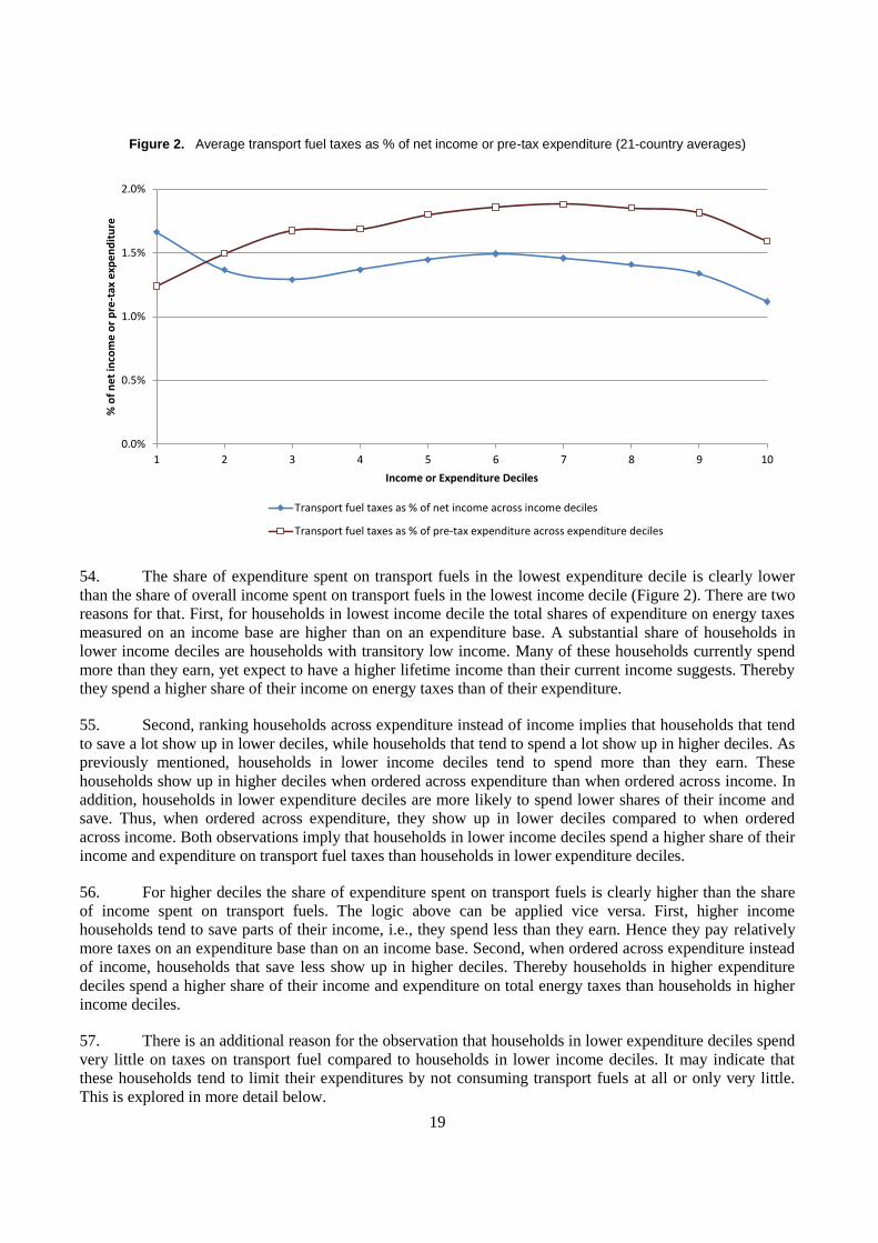
53. Figure 2 shows the tax burden on transport fuels on an income basis (light blue line with diamonds)

and on expenditure basis (dark red line with empty squares) as an unweighted average for all countries

analysed. On an income basis there is no monotonic pattern for taxes on transport fuels: The transport fuel tax

burden decreases from the first to the second the third decile, while it then increases to the sixth decile before

it decreases again to the tenth decile. On an expenditure base there is a progressive trend, although the pattern

here is not strictly monotonic either, given that there is a noticeable decline in the expenditure share for the

highest decile.

22. Expenditure related results are presented in terms of pre-tax expenditure as opposed to post-tax expenditure.

There is no obvious reason for preferring one over the other measure with respect to ad-quantum excise taxes. In

the case of VAT presenting results in terms of pre-tax expenditure provides a direct comparison of effective tax

burdens with standard rates (OECD, 2014a). To allow for a comparison of results in this paper with those in the

OECD (2014a) study on VAT results are presented in terms of pre-tax expenditure.

19

Figure 2. Average transport fuel taxes as % of net income or pre-tax expenditure (21-country averages)

54. The share of expenditure spent on transport fuels in the lowest expenditure decile is clearly lower

than the share of overall income spent on transport fuels in the lowest income decile (Figure 2). There are two

reasons for that. First, for households in lowest income decile the total shares of expenditure on energy taxes

measured on an income base are higher than on an expenditure base. A substantial share of households in

lower income deciles are households with transitory low income. Many of these households currently spend

more than they earn, yet expect to have a higher lifetime income than their current income suggests. Thereby

they spend a higher share of their income on energy taxes than of their expenditure.

55. Second, ranking households across expenditure instead of income implies that households that tend

to save a lot show up in lower deciles, while households that tend to spend a lot show up in higher deciles. As

previously mentioned, households in lower income deciles tend to spend more than they earn. These

households show up in higher deciles when ordered across expenditure than when ordered across income. In

addition, households in lower expenditure deciles are more likely to spend lower shares of their income and

save. Thus, when ordered across expenditure, they show up in lower deciles compared to when ordered

across income. Both observations imply that households in lower income deciles spend a higher share of their

income and expenditure on transport fuel taxes than households in lower expenditure deciles.

56. For higher deciles the share of expenditure spent on transport fuels is clearly higher than the share

of income spent on transport fuels. The logic above can be applied vice versa. First, higher income

households tend to save parts of their income, i.e., they spend less than they earn. Hence they pay relatively

more taxes on an expenditure base than on an income base. Second, when ordered across expenditure instead

of income, households that save less show up in higher deciles. Thereby households in higher expenditure

deciles spend a higher share of their income and expenditure on total energy taxes than households in higher

income deciles.

57. There is an additional reason for the observation that households in lower expenditure deciles spend

very little on taxes on transport fuel compared to households in lower income deciles. It may indicate that

these households tend to limit their expenditures by not consuming transport fuels at all or only very little.

This is explored in more detail below.

0.0%

0.5%

1.0%

1.5%

2.0%

1 2 3 4 5 6 7 8 9 10

% o

f n

et

inco

me

or

pre

-tax

exp

en

dit

ure

Income or Expenditure Deciles

Transport fuel taxes as % of net income across income deciles

Transport fuel taxes as % of pre-tax expenditure across expenditure deciles

20

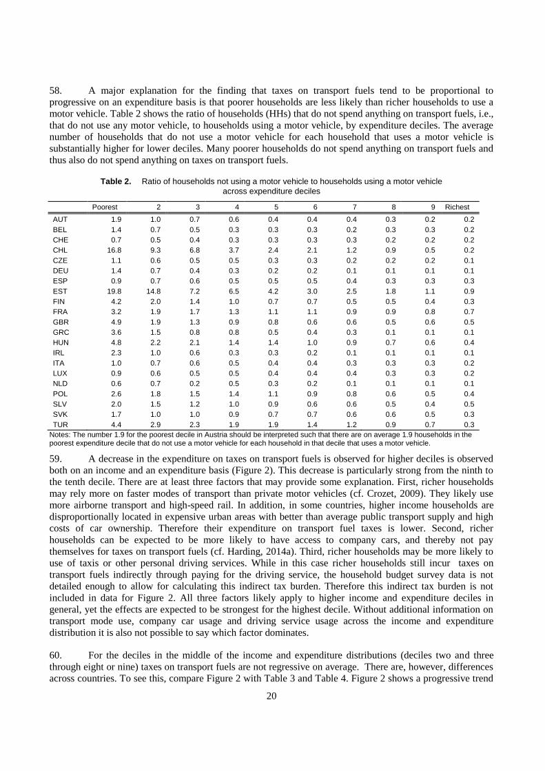
58. A major explanation for the finding that taxes on transport fuels tend to be proportional to

progressive on an expenditure basis is that poorer households are less likely than richer households to use a

motor vehicle. Table 2 shows the ratio of households (HHs) that do not spend anything on transport fuels, i.e.,

that do not use any motor vehicle, to households using a motor vehicle, by expenditure deciles. The average

number of households that do not use a motor vehicle for each household that uses a motor vehicle is

substantially higher for lower deciles. Many poorer households do not spend anything on transport fuels and

thus also do not spend anything on taxes on transport fuels.

Table 2. Ratio of households not using a motor vehicle to households using a motor vehicle

across expenditure deciles

Poorest 2 3 4 5 6 7 8 9 Richest

AUT 1.9 1.0 0.7 0.6 0.4 0.4 0.4 0.3 0.2 0.2

BEL 1.4 0.7 0.5 0.3 0.3 0.3 0.2 0.3 0.3 0.2

CHE 0.7 0.5 0.4 0.3 0.3 0.3 0.3 0.2 0.2 0.2

CHL 16.8 9.3 6.8 3.7 2.4 2.1 1.2 0.9 0.5 0.2

CZE 1.1 0.6 0.5 0.5 0.3 0.3 0.2 0.2 0.2 0.1

DEU 1.4 0.7 0.4 0.3 0.2 0.2 0.1 0.1 0.1 0.1

ESP 0.9 0.7 0.6 0.5 0.5 0.5 0.4 0.3 0.3 0.3

EST 19.8 14.8 7.2 6.5 4.2 3.0 2.5 1.8 1.1 0.9

FIN 4.2 2.0 1.4 1.0 0.7 0.7 0.5 0.5 0.4 0.3

FRA 3.2 1.9 1.7 1.3 1.1 1.1 0.9 0.9 0.8 0.7

GBR 4.9 1.9 1.3 0.9 0.8 0.6 0.6 0.5 0.6 0.5

GRC 3.6 1.5 0.8 0.8 0.5 0.4 0.3 0.1 0.1 0.1

HUN 4.8 2.2 2.1 1.4 1.4 1.0 0.9 0.7 0.6 0.4

IRL 2.3 1.0 0.6 0.3 0.3 0.2 0.1 0.1 0.1 0.1

ITA 1.0 0.7 0.6 0.5 0.4 0.4 0.3 0.3 0.3 0.2

LUX 0.9 0.6 0.5 0.5 0.4 0.4 0.4 0.3 0.3 0.2

NLD 0.6 0.7 0.2 0.5 0.3 0.2 0.1 0.1 0.1 0.1

POL 2.6 1.8 1.5 1.4 1.1 0.9 0.8 0.6 0.5 0.4

SLV 2.0 1.5 1.2 1.0 0.9 0.6 0.6 0.5 0.4 0.5

SVK 1.7 1.0 1.0 0.9 0.7 0.7 0.6 0.6 0.5 0.3

TUR 4.4 2.9 2.3 1.9 1.9 1.4 1.2 0.9 0.7 0.3

Notes: The number 1.9 for the poorest decile in Austria should be interpreted such that there are on average 1.9 households in the poorest expenditure decile that do not use a motor vehicle for each household in that decile that uses a motor vehicle.

59. A decrease in the expenditure on taxes on transport fuels is observed for higher deciles is observed

both on an income and an expenditure basis (Figure 2). This decrease is particularly strong from the ninth to

the tenth decile. There are at least three factors that may provide some explanation. First, richer households

may rely more on faster modes of transport than private motor vehicles (cf. Crozet, 2009). They likely use

more airborne transport and high-speed rail. In addition, in some countries, higher income households are

disproportionally located in expensive urban areas with better than average public transport supply and high

costs of car ownership. Therefore their expenditure on transport fuel taxes is lower. Second, richer

households can be expected to be more likely to have access to company cars, and thereby not pay

themselves for taxes on transport fuels (cf. Harding, 2014a). Third, richer households may be more likely to

use of taxis or other personal driving services. While in this case richer households still incur taxes on

transport fuels indirectly through paying for the driving service, the household budget survey data is not

detailed enough to allow for calculating this indirect tax burden. Therefore this indirect tax burden is not

included in data for Figure 2. All three factors likely apply to higher income and expenditure deciles in

general, yet the effects are expected to be strongest for the highest decile. Without additional information on

transport mode use, company car usage and driving service usage across the income and expenditure

distribution it is also not possible to say which factor dominates.

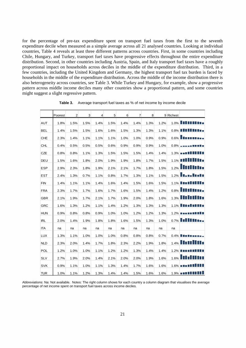
60. For the deciles in the middle of the income and expenditure distributions (deciles two and three

through eight or nine) taxes on transport fuels are not regressive on average. There are, however, differences

across countries. To see this, compare Figure 2 with Table 3 and Table 4. Figure 2 shows a progressive trend

21

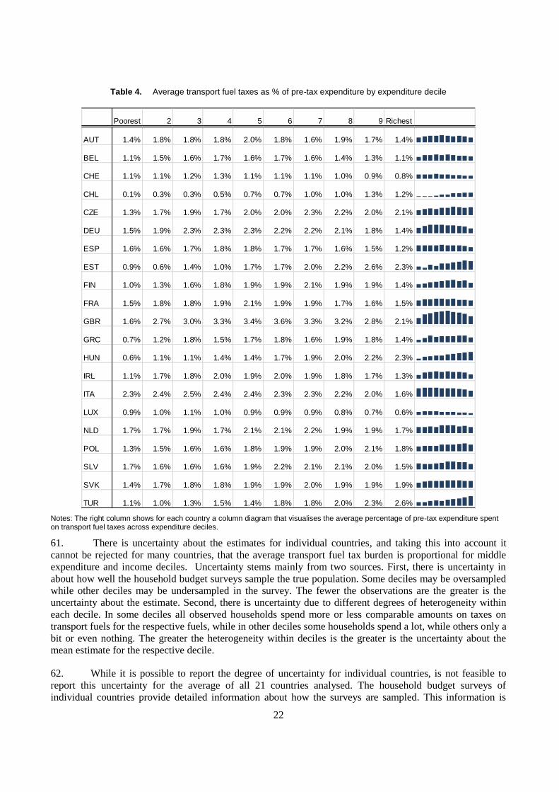
for the percentage of pre-tax expenditure spent on transport fuel taxes from the first to the seventh

expenditure decile when measured as a simple average across all 21 analysed countries. Looking at individual

countries, Table 4 reveals at least three different patterns across countries. First, in some countries including

Chile, Hungary, and Turkey, transport fuel taxes have progressive effects throughout the entire expenditure

distribution. Second, in other countries including Austria, Spain, and Italy transport fuel taxes have a roughly

proportional impact on households across deciles in the middle of the expenditure distribution. Third, in a

few countries, including the United Kingdom and Germany, the highest transport fuel tax burden is faced by

households in the middle of the expenditure distribution. Across the middle of the income distribution there is

also heterogeneity across countries, see Table 3. While Turkey and Hungary, for example, show a progressive

pattern across middle income deciles many other countries show a proportional pattern, and some countries

might suggest a slight regressive pattern.

Table 3. Average transport fuel taxes as % of net income by income decile

Abbreviations: Na: Not available. Notes: The right column shows for each country a column diagram that visualises the average percentage of net income spent on transport fuel taxes across income deciles.

Poorest 2 3 4 5 6 7 8 9 Richest

AUT 1.8% 1.5% 1.5% 1.4% 1.5% 1.4% 1.4% 1.3% 1.2% 1.0%

BEL 1.4% 1.5% 1.5% 1.6% 1.6% 1.5% 1.3% 1.3% 1.1% 0.8%

CHE 2.3% 1.4% 1.1% 1.1% 1.1% 1.0% 1.0% 0.9% 0.9% 0.6%

CHL 0.4% 0.5% 0.5% 0.5% 0.6% 0.9% 0.9% 0.9% 1.0% 0.8%

CZE 0.8% 0.8% 1.1% 1.3% 1.5% 1.5% 1.5% 1.4% 1.4% 1.3%

DEU 1.5% 1.6% 1.8% 2.0% 1.9% 1.9% 1.8% 1.7% 1.5% 1.1%

ESP 2.9% 2.3% 1.8% 1.9% 2.1% 2.1% 1.7% 1.8% 1.5% 1.2%

EST 2.4% 1.3% 0.7% 1.1% 0.8% 1.7% 1.3% 1.1% 1.5% 1.2%

FIN 1.4% 1.1% 1.1% 1.4% 1.6% 1.4% 1.5% 1.6% 1.5% 1.1%

FRA 2.3% 1.7% 1.7% 1.6% 1.7% 1.6% 1.5% 1.4% 1.2% 0.8%

GBR 2.1% 1.9% 1.7% 2.1% 1.7% 1.9% 2.0% 1.8% 1.6% 1.3%

GRC 1.6% 1.3% 1.2% 1.1% 1.4% 1.2% 1.3% 1.3% 1.3% 1.1%

HUN 0.9% 0.8% 0.8% 0.9% 1.0% 1.0% 1.2% 1.2% 1.3% 1.2%

IRL 2.0% 1.4% 1.9% 1.8% 1.8% 1.6% 1.5% 1.3% 1.0% 0.7%

ITA na na na na na na na na na na

LUX 1.3% 1.1% 1.0% 1.0% 1.0% 0.8% 0.8% 0.8% 0.7% 0.4%

NLD 2.3% 2.0% 1.4% 1.7% 1.8% 2.3% 2.2% 1.9% 1.8% 1.4%

POL 1.2% 1.0% 1.0% 1.1% 1.2% 1.2% 1.3% 1.4% 1.4% 1.2%

SLV 2.7% 1.9% 2.0% 1.4% 2.1% 2.0% 2.0% 1.9% 1.6% 1.6%

SVK 0.9% 1.1% 1.0% 1.1% 1.3% 1.4% 1.7% 1.6% 1.6% 1.6%

TUR 1.0% 1.1% 1.2% 1.3% 1.4% 1.4% 1.5% 1.6% 1.6% 1.9%

22

Table 4. Average transport fuel taxes as % of pre-tax expenditure by expenditure decile

Notes: The right column shows for each country a column diagram that visualises the average percentage of pre-tax expenditure spent on transport fuel taxes across expenditure deciles.

61. There is uncertainty about the estimates for individual countries, and taking this into account it

cannot be rejected for many countries, that the average transport fuel tax burden is proportional for middle

expenditure and income deciles. Uncertainty stems mainly from two sources. First, there is uncertainty in

about how well the household budget surveys sample the true population. Some deciles may be oversampled

while other deciles may be undersampled in the survey. The fewer the observations are the greater is the

uncertainty about the estimate. Second, there is uncertainty due to different degrees of heterogeneity within

each decile. In some deciles all observed households spend more or less comparable amounts on taxes on

transport fuels for the respective fuels, while in other deciles some households spend a lot, while others only a

bit or even nothing. The greater the heterogeneity within deciles is the greater is the uncertainty about the

mean estimate for the respective decile.

62. While it is possible to report the degree of uncertainty for individual countries, is not feasible to

report this uncertainty for the average of all 21 countries analysed. The household budget surveys of

individual countries provide detailed information about how the surveys are sampled. This information is

Poorest 2 3 4 5 6 7 8 9 Richest

AUT 1.4% 1.8% 1.8% 1.8% 2.0% 1.8% 1.6% 1.9% 1.7% 1.4%

BEL 1.1% 1.5% 1.6% 1.7% 1.6% 1.7% 1.6% 1.4% 1.3% 1.1%

CHE 1.1% 1.1% 1.2% 1.3% 1.1% 1.1% 1.1% 1.0% 0.9% 0.8%

CHL 0.1% 0.3% 0.3% 0.5% 0.7% 0.7% 1.0% 1.0% 1.3% 1.2%

CZE 1.3% 1.7% 1.9% 1.7% 2.0% 2.0% 2.3% 2.2% 2.0% 2.1%

DEU 1.5% 1.9% 2.3% 2.3% 2.3% 2.2% 2.2% 2.1% 1.8% 1.4%

ESP 1.6% 1.6% 1.7% 1.8% 1.8% 1.7% 1.7% 1.6% 1.5% 1.2%

EST 0.9% 0.6% 1.4% 1.0% 1.7% 1.7% 2.0% 2.2% 2.6% 2.3%

FIN 1.0% 1.3% 1.6% 1.8% 1.9% 1.9% 2.1% 1.9% 1.9% 1.4%

FRA 1.5% 1.8% 1.8% 1.9% 2.1% 1.9% 1.9% 1.7% 1.6% 1.5%

GBR 1.6% 2.7% 3.0% 3.3% 3.4% 3.6% 3.3% 3.2% 2.8% 2.1%

GRC 0.7% 1.2% 1.8% 1.5% 1.7% 1.8% 1.6% 1.9% 1.8% 1.4%

HUN 0.6% 1.1% 1.1% 1.4% 1.4% 1.7% 1.9% 2.0% 2.2% 2.3%

IRL 1.1% 1.7% 1.8% 2.0% 1.9% 2.0% 1.9% 1.8% 1.7% 1.3%

ITA 2.3% 2.4% 2.5% 2.4% 2.4% 2.3% 2.3% 2.2% 2.0% 1.6%

LUX 0.9% 1.0% 1.1% 1.0% 0.9% 0.9% 0.9% 0.8% 0.7% 0.6%

NLD 1.7% 1.7% 1.9% 1.7% 2.1% 2.1% 2.2% 1.9% 1.9% 1.7%

POL 1.3% 1.5% 1.6% 1.6% 1.8% 1.9% 1.9% 2.0% 2.1% 1.8%

SLV 1.7% 1.6% 1.6% 1.6% 1.9% 2.2% 2.1% 2.1% 2.0% 1.5%

SVK 1.4% 1.7% 1.8% 1.8% 1.9% 1.9% 2.0% 1.9% 1.9% 1.9%

TUR 1.1% 1.0% 1.3% 1.5% 1.4% 1.8% 1.8% 2.0% 2.3% 2.6%

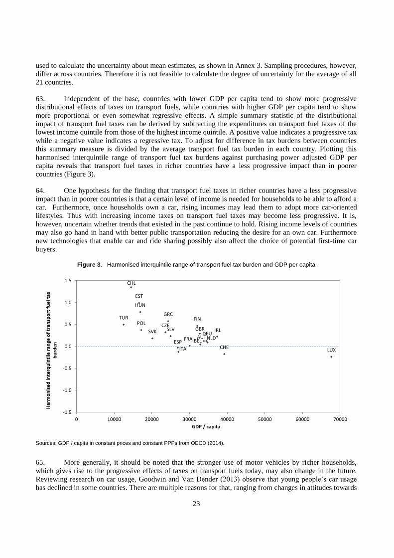
23

used to calculate the uncertainty about mean estimates, as shown in Annex 3. Sampling procedures, however,

differ across countries. Therefore it is not feasible to calculate the degree of uncertainty for the average of all

21 countries.

63. Independent of the base, countries with lower GDP per capita tend to show more progressive

distributional effects of taxes on transport fuels, while countries with higher GDP per capita tend to show

more proportional or even somewhat regressive effects. A simple summary statistic of the distributional

impact of transport fuel taxes can be derived by subtracting the expenditures on transport fuel taxes of the

lowest income quintile from those of the highest income quintile. A positive value indicates a progressive tax

while a negative value indicates a regressive tax. To adjust for difference in tax burdens between countries

this summary measure is divided by the average transport fuel tax burden in each country. Plotting this

harmonised interquintile range of transport fuel tax burdens against purchasing power adjusted GDP per

capita reveals that transport fuel taxes in richer countries have a less progressive impact than in poorer

countries (Figure 3).

64. One hypothesis for the finding that transport fuel taxes in richer countries have a less progressive

impact than in poorer countries is that a certain level of income is needed for households to be able to afford a

car. Furthermore, once households own a car, rising incomes may lead them to adopt more car-oriented

lifestyles. Thus with increasing income taxes on transport fuel taxes may become less progressive. It is,

however, uncertain whether trends that existed in the past continue to hold. Rising income levels of countries

may also go hand in hand with better public transportation reducing the desire for an own car. Furthermore

new technologies that enable car and ride sharing possibly also affect the choice of potential first-time car

buyers.

Figure 3. Harmonised interquintile range of transport fuel tax burden and GDP per capita

Sources: GDP / capita in constant prices and constant PPPs from OECD (2014).

65. More generally, it should be noted that the stronger use of motor vehicles by richer households,

which gives rise to the progressive effects of taxes on transport fuels today, may also change in the future.

Reviewing research on car usage, Goodwin and Van Dender (2013) observe that young people’s car usage

has declined in some countries. There are multiple reasons for that, ranging from changes in attitudes towards

AUTBEL

CHE

CHL

CZE

DEU

ESP

EST

FIN

FRA

GBR

GRC

HUN

IRL

ITA LUX

NLD

POLSLVSVK

TUR

-1.5

-1.0

-0.5

0.0

0.5

1.0

1.5

0 10000 20000 30000 40000 50000 60000 70000

Har

mo

nis

ed

inte

rqu

inti

le r

ange

of

tran

spo

rt f

ue

l tax

b

urd

en

GDP / capita

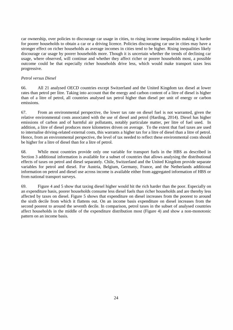
24

car ownership, over policies to discourage car usage in cities, to rising income inequalities making it harder

for poorer households to obtain a car or a driving licence. Policies discouraging car use in cities may have a

stronger effect on richer households as average incomes in cities tend to be higher. Rising inequalities likely

discourage car usage by poorer households more. Though it is uncertain whether the trends of declining car

usage, where observed, will continue and whether they affect richer or poorer households most, a possible

outcome could be that especially richer households drive less, which would make transport taxes less

progressive.

Petrol versus Diesel

66. All 21 analysed OECD countries except Switzerland and the United Kingdom tax diesel at lower

rates than petrol per litre. Taking into account that the energy and carbon content of a litre of diesel is higher

than of a litre of petrol, all countries analysed tax petrol higher than diesel per unit of energy or carbon

emissions.

67. From an environmental perspective, the lower tax rate on diesel fuel is not warranted, given the

relative environmental costs associated with the use of diesel and petrol (Harding, 2014). Diesel has higher

emissions of carbon and of harmful air pollutants, notably particulate matter, per litre of fuel used. In

addition, a litre of diesel produces more kilometres driven on average. To the extent that fuel taxes are used

to internalise driving-related external costs, this warrants a higher tax for a litre of diesel than a litre of petrol.

Hence, from an environmental perspective, the level of tax needed to reflect these environmental costs should

be higher for a litre of diesel than for a litre of petrol.

68. While most countries provide only one variable for transport fuels in the HBS as described in

Section 3 additional information is available for a subset of countries that allows analysing the distributional

effects of taxes on petrol and diesel separately. Chile, Switzerland and the United Kingdom provide separate

variables for petrol and diesel. For Austria, Belgium, Germany, France, and the Netherlands additional

information on petrol and diesel use across income is available either from aggregated information of HBS or

from national transport surveys.

69. Figure 4 and 5 show that taxing diesel higher would hit the rich harder than the poor. Especially on

an expenditure basis, poorer households consume less diesel fuels than richer households and are thereby less

affected by taxes on diesel. Figure 5 shows that expenditure on diesel increases from the poorest to around

the sixth decile from which it flattens out. On an income basis expenditure on diesel increases from the

second poorest to around the seventh decile. In comparison, petrol taxes in the subset of analysed countries

affect households in the middle of the expenditure distribution most (Figure 4) and show a non-monotonic

pattern on an income basis.

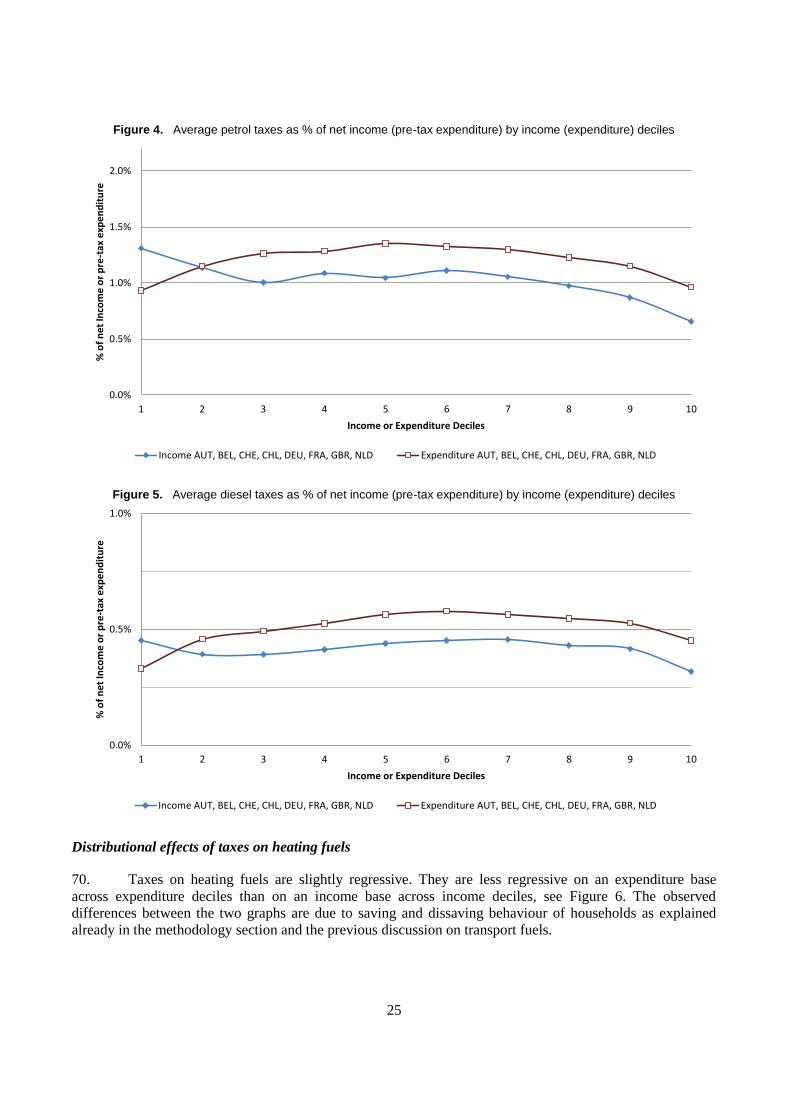
25

Figure 4. Average petrol taxes as % of net income (pre-tax expenditure) by income (expenditure) deciles

Figure 5. Average diesel taxes as % of net income (pre-tax expenditure) by income (expenditure) deciles

Distributional effects of taxes on heating fuels

70. Taxes on heating fuels are slightly regressive. They are less regressive on an expenditure base

across expenditure deciles than on an income base across income deciles, see Figure 6. The observed

differences between the two graphs are due to saving and dissaving behaviour of households as explained

already in the methodology section and the previous discussion on transport fuels.

0.0%

0.5%

1.0%

1.5%

2.0%

1 2 3 4 5 6 7 8 9 10

% o

f n

et

Inco

me

or

pre

-tax

exp

en

dit

ure

Income or Expenditure Deciles

Income AUT, BEL, CHE, CHL, DEU, FRA, GBR, NLD Expenditure AUT, BEL, CHE, CHL, DEU, FRA, GBR, NLD

0.0%

0.5%

1.0%

1 2 3 4 5 6 7 8 9 10

% o

f n

et

Inco

me

or

pre

-tax

exp

en

dit

ure

Income or Expenditure Deciles

Income AUT, BEL, CHE, CHL, DEU, FRA, GBR, NLD Expenditure AUT, BEL, CHE, CHL, DEU, FRA, GBR, NLD

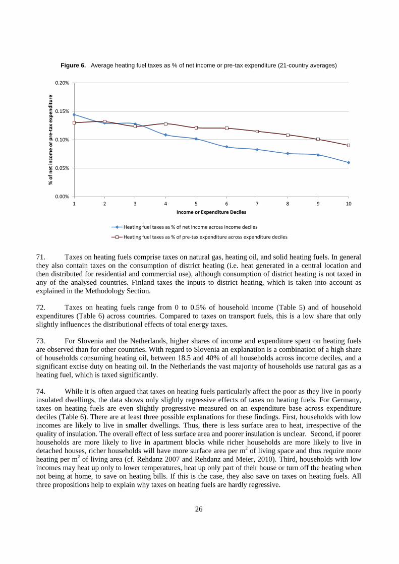
26

Figure 6. Average heating fuel taxes as % of net income or pre-tax expenditure (21-country averages)

71. Taxes on heating fuels comprise taxes on natural gas, heating oil, and solid heating fuels. In general

they also contain taxes on the consumption of district heating (i.e. heat generated in a central location and

then distributed for residential and commercial use), although consumption of district heating is not taxed in

any of the analysed countries. Finland taxes the inputs to district heating, which is taken into account as

explained in the Methodology Section.

72. Taxes on heating fuels range from 0 to 0.5% of household income (Table 5) and of household

expenditures (Table 6) across countries. Compared to taxes on transport fuels, this is a low share that only

slightly influences the distributional effects of total energy taxes.

73. For Slovenia and the Netherlands, higher shares of income and expenditure spent on heating fuels

are observed than for other countries. With regard to Slovenia an explanation is a combination of a high share

of households consuming heating oil, between 18.5 and 40% of all households across income deciles, and a

significant excise duty on heating oil. In the Netherlands the vast majority of households use natural gas as a

heating fuel, which is taxed significantly.

74. While it is often argued that taxes on heating fuels particularly affect the poor as they live in poorly

insulated dwellings, the data shows only slightly regressive effects of taxes on heating fuels. For Germany,

taxes on heating fuels are even slightly progressive measured on an expenditure base across expenditure

deciles (Table 6). There are at least three possible explanations for these findings. First, households with low

incomes are likely to live in smaller dwellings. Thus, there is less surface area to heat, irrespective of the

quality of insulation. The overall effect of less surface area and poorer insulation is unclear. Second, if poorer

households are more likely to live in apartment blocks while richer households are more likely to live in

detached houses, richer households will have more surface area per m2 of living space and thus require more

heating per m2 of living area (cf. Rehdanz 2007 and Rehdanz and Meier, 2010). Third, households with low

incomes may heat up only to lower temperatures, heat up only part of their house or turn off the heating when

not being at home, to save on heating bills. If this is the case, they also save on taxes on heating fuels. All

three propositions help to explain why taxes on heating fuels are hardly regressive.

0.00%

0.05%

0.10%

0.15%

0.20%

1 2 3 4 5 6 7 8 9 10

% o

f n

et

inco

me

or

pre

-tax

exp

en

dit

ure

Income or Expenditure Deciles

Heating fuel taxes as % of net income across income deciles

Heating fuel taxes as % of pre-tax expenditure across expenditure deciles

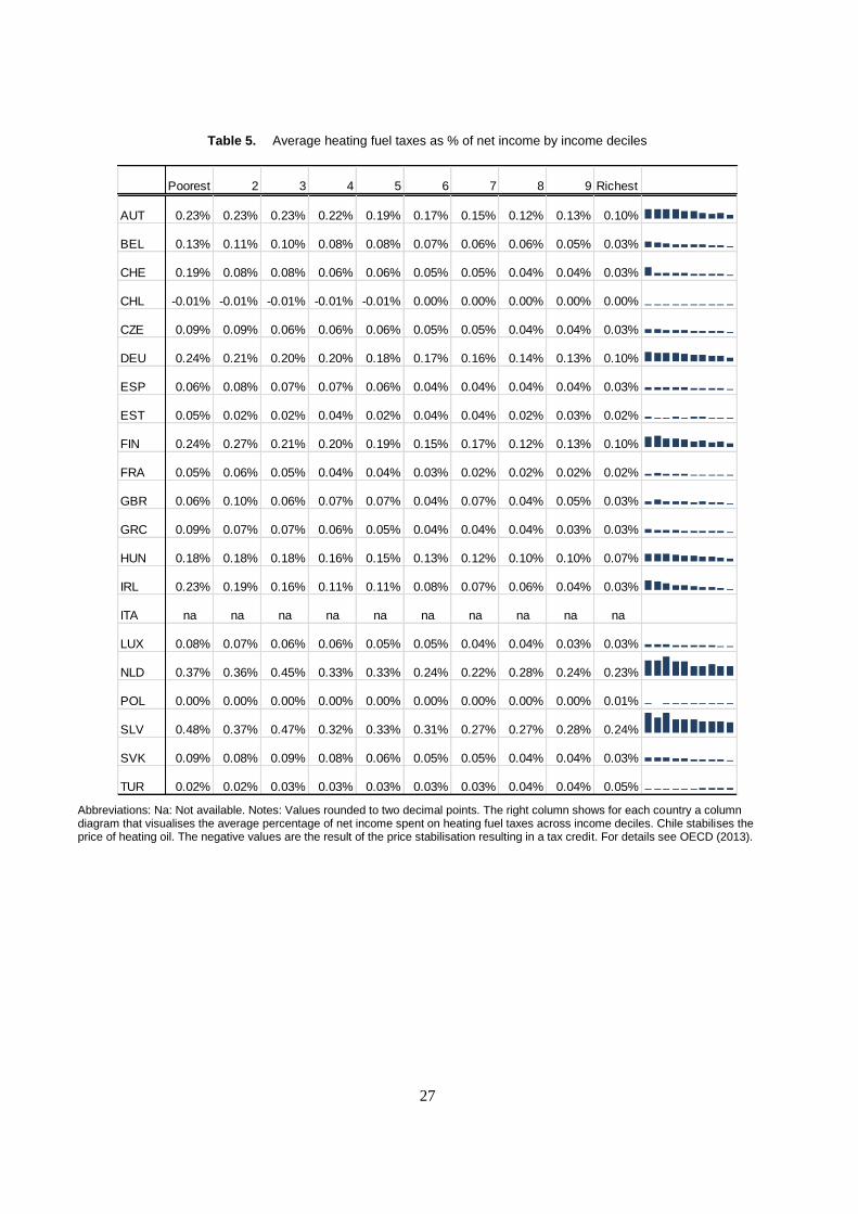
27

Table 5. Average heating fuel taxes as % of net income by income deciles

Abbreviations: Na: Not available. Notes: Values rounded to two decimal points. The right column shows for each country a column diagram that visualises the average percentage of net income spent on heating fuel taxes across income deciles. Chile stabilises the price of heating oil. The negative values are the result of the price stabilisation resulting in a tax credit. For details see OECD (2013).

Poorest 2 3 4 5 6 7 8 9 Richest

AUT 0.23% 0.23% 0.23% 0.22% 0.19% 0.17% 0.15% 0.12% 0.13% 0.10%

BEL 0.13% 0.11% 0.10% 0.08% 0.08% 0.07% 0.06% 0.06% 0.05% 0.03%

CHE 0.19% 0.08% 0.08% 0.06% 0.06% 0.05% 0.05% 0.04% 0.04% 0.03%

CHL -0.01% -0.01% -0.01% -0.01% -0.01% 0.00% 0.00% 0.00% 0.00% 0.00%

CZE 0.09% 0.09% 0.06% 0.06% 0.06% 0.05% 0.05% 0.04% 0.04% 0.03%

DEU 0.24% 0.21% 0.20% 0.20% 0.18% 0.17% 0.16% 0.14% 0.13% 0.10%

ESP 0.06% 0.08% 0.07% 0.07% 0.06% 0.04% 0.04% 0.04% 0.04% 0.03%

EST 0.05% 0.02% 0.02% 0.04% 0.02% 0.04% 0.04% 0.02% 0.03% 0.02%

FIN 0.24% 0.27% 0.21% 0.20% 0.19% 0.15% 0.17% 0.12% 0.13% 0.10%

FRA 0.05% 0.06% 0.05% 0.04% 0.04% 0.03% 0.02% 0.02% 0.02% 0.02%

GBR 0.06% 0.10% 0.06% 0.07% 0.07% 0.04% 0.07% 0.04% 0.05% 0.03%

GRC 0.09% 0.07% 0.07% 0.06% 0.05% 0.04% 0.04% 0.04% 0.03% 0.03%

HUN 0.18% 0.18% 0.18% 0.16% 0.15% 0.13% 0.12% 0.10% 0.10% 0.07%

IRL 0.23% 0.19% 0.16% 0.11% 0.11% 0.08% 0.07% 0.06% 0.04% 0.03%

ITA na na na na na na na na na na

LUX 0.08% 0.07% 0.06% 0.06% 0.05% 0.05% 0.04% 0.04% 0.03% 0.03%

NLD 0.37% 0.36% 0.45% 0.33% 0.33% 0.24% 0.22% 0.28% 0.24% 0.23%

POL 0.00% 0.00% 0.00% 0.00% 0.00% 0.00% 0.00% 0.00% 0.00% 0.01%

SLV 0.48% 0.37% 0.47% 0.32% 0.33% 0.31% 0.27% 0.27% 0.28% 0.24%

SVK 0.09% 0.08% 0.09% 0.08% 0.06% 0.05% 0.05% 0.04% 0.04% 0.03%

TUR 0.02% 0.02% 0.03% 0.03% 0.03% 0.03% 0.03% 0.04% 0.04% 0.05%

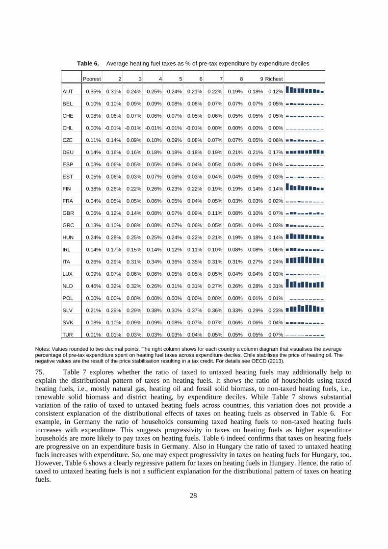
28

Table 6. Average heating fuel taxes as % of pre-tax expenditure by expenditure deciles

Notes: Values rounded to two decimal points. The right column shows for each country a column diagram that visualises the average percentage of pre-tax expenditure spent on heating fuel taxes across expenditure deciles. Chile stabilises the price of heating oil. The negative values are the result of the price stabilisation resulting in a tax credit. For details see OECD (2013).

75. Table 7 explores whether the ratio of taxed to untaxed heating fuels may additionally help to

explain the distributional pattern of taxes on heating fuels. It shows the ratio of households using taxed

heating fuels, i.e., mostly natural gas, heating oil and fossil solid biomass, to non-taxed heating fuels, i.e.,

renewable solid biomass and district heating, by expenditure deciles. While Table 7 shows substantial

variation of the ratio of taxed to untaxed heating fuels across countries, this variation does not provide a

consistent explanation of the distributional effects of taxes on heating fuels as observed in Table 6. For

example, in Germany the ratio of households consuming taxed heating fuels to non-taxed heating fuels

increases with expenditure. This suggests progressivity in taxes on heating fuels as higher expenditure

households are more likely to pay taxes on heating fuels. Table 6 indeed confirms that taxes on heating fuels

are progressive on an expenditure basis in Germany. Also in Hungary the ratio of taxed to untaxed heating

fuels increases with expenditure. So, one may expect progressivity in taxes on heating fuels for Hungary, too.

However, Table 6 shows a clearly regressive pattern for taxes on heating fuels in Hungary. Hence, the ratio of

taxed to untaxed heating fuels is not a sufficient explanation for the distributional pattern of taxes on heating

fuels.

Poorest 2 3 4 5 6 7 8 9 Richest

AUT 0.35% 0.31% 0.24% 0.25% 0.24% 0.21% 0.22% 0.19% 0.18% 0.12%

BEL 0.10% 0.10% 0.09% 0.09% 0.08% 0.08% 0.07% 0.07% 0.07% 0.05%

CHE 0.08% 0.06% 0.07% 0.06% 0.07% 0.05% 0.06% 0.05% 0.05% 0.05%

CHL 0.00% -0.01% -0.01% -0.01% -0.01% -0.01% 0.00% 0.00% 0.00% 0.00%

CZE 0.11% 0.14% 0.09% 0.10% 0.09% 0.08% 0.07% 0.07% 0.05% 0.06%

DEU 0.14% 0.16% 0.16% 0.18% 0.18% 0.18% 0.19% 0.21% 0.21% 0.17%

ESP 0.03% 0.06% 0.05% 0.05% 0.04% 0.04% 0.05% 0.04% 0.04% 0.04%

EST 0.05% 0.06% 0.03% 0.07% 0.06% 0.03% 0.04% 0.04% 0.05% 0.03%

FIN 0.38% 0.26% 0.22% 0.26% 0.23% 0.22% 0.19% 0.19% 0.14% 0.14%

FRA 0.04% 0.05% 0.05% 0.06% 0.05% 0.04% 0.05% 0.03% 0.03% 0.02%

GBR 0.06% 0.12% 0.14% 0.08% 0.07% 0.09% 0.11% 0.08% 0.10% 0.07%

GRC 0.13% 0.10% 0.08% 0.08% 0.07% 0.06% 0.05% 0.05% 0.04% 0.03%

HUN 0.24% 0.28% 0.25% 0.25% 0.24% 0.22% 0.21% 0.19% 0.18% 0.14%

IRL 0.14% 0.17% 0.15% 0.14% 0.12% 0.11% 0.10% 0.08% 0.08% 0.06%

ITA 0.26% 0.29% 0.31% 0.34% 0.36% 0.35% 0.31% 0.31% 0.27% 0.24%

LUX 0.09% 0.07% 0.06% 0.06% 0.05% 0.05% 0.05% 0.04% 0.04% 0.03%

NLD 0.46% 0.32% 0.32% 0.26% 0.31% 0.31% 0.27% 0.26% 0.28% 0.31%

POL 0.00% 0.00% 0.00% 0.00% 0.00% 0.00% 0.00% 0.00% 0.01% 0.01%

SLV 0.21% 0.29% 0.29% 0.38% 0.30% 0.37% 0.36% 0.33% 0.29% 0.23%

SVK 0.08% 0.10% 0.09% 0.09% 0.08% 0.07% 0.07% 0.06% 0.06% 0.04%

TUR 0.01% 0.01% 0.03% 0.03% 0.03% 0.04% 0.05% 0.05% 0.05% 0.07%

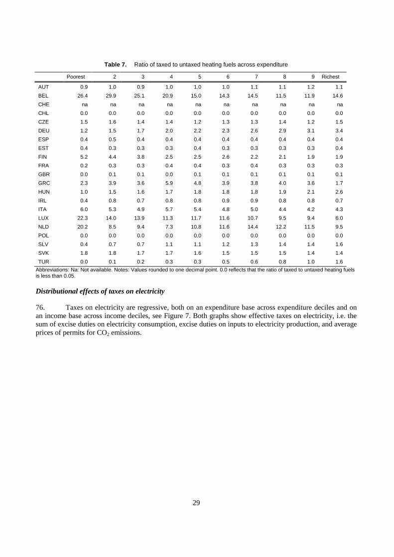
29

Table 7. Ratio of taxed to untaxed heating fuels across expenditure

Poorest 2 3 4 5 6 7 8 9 Richest

AUT 0.9 1.0 0.9 1.0 1.0 1.0 1.1 1.1 1.2 1.1

BEL 26.4 29.9 25.1 20.9 15.0 14.3 14.5 11.5 11.9 14.6

CHE na na na na na na na na na na

CHL 0.0 0.0 0.0 0.0 0.0 0.0 0.0 0.0 0.0 0.0

CZE 1.5 1.6 1.4 1.4 1.2 1.3 1.3 1.4 1.2 1.5

DEU 1.2 1.5 1.7 2.0 2.2 2.3 2.6 2.9 3.1 3.4

ESP 0.4 0.5 0.4 0.4 0.4 0.4 0.4 0.4 0.4 0.4

EST 0.4 0.3 0.3 0.3 0.4 0.3 0.3 0.3 0.3 0.4

FIN 5.2 4.4 3.8 2.5 2.5 2.6 2.2 2.1 1.9 1.9

FRA 0.2 0.3 0.3 0.4 0.4 0.3 0.4 0.3 0.3 0.3

GBR 0.0 0.1 0.1 0.0 0.1 0.1 0.1 0.1 0.1 0.1

GRC 2.3 3.9 3.6 5.9 4.8 3.9 3.8 4.0 3.6 1.7

HUN 1.0 1.5 1.6 1.7 1.8 1.8 1.8 1.9 2.1 2.6

IRL 0.4 0.8 0.7 0.8 0.8 0.9 0.9 0.8 0.8 0.7

ITA 6.0 5.3 4.9 5.7 5.4 4.8 5.0 4.4 4.2 4.3

LUX 22.3 14.0 13.9 11.3 11.7 11.6 10.7 9.5 9.4 6.0

NLD 20.2 8.5 9.4 7.3 10.8 11.6 14.4 12.2 11.5 9.5

POL 0.0 0.0 0.0 0.0 0.0 0.0 0.0 0.0 0.0 0.0

SLV 0.4 0.7 0.7 1.1 1.1 1.2 1.3 1.4 1.4 1.6

SVK 1.8 1.8 1.7 1.7 1.6 1.5 1.5 1.5 1.4 1.4

TUR 0.0 0.1 0.2 0.3 0.3 0.5 0.6 0.8 1.0 1.6

Abbreviations: Na: Not available. Notes: Values rounded to one decimal point. 0.0 reflects that the ratio of taxed to untaxed heating fuels is less than 0.05.

Distributional effects of taxes on electricity

76. Taxes on electricity are regressive, both on an expenditure base across expenditure deciles and on

an income base across income deciles, see Figure 7. Both graphs show effective taxes on electricity, i.e. the

sum of excise duties on electricity consumption, excise duties on inputs to electricity production, and average

prices of permits for CO2 emissions.

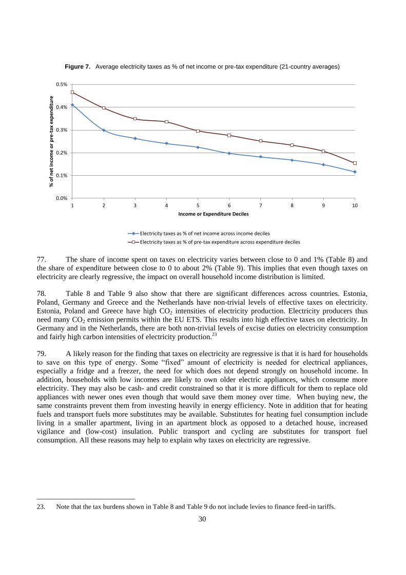
30

Figure 7. Average electricity taxes as % of net income or pre-tax expenditure (21-country averages)

77. The share of income spent on taxes on electricity varies between close to 0 and 1% (Table 8) and

the share of expenditure between close to 0 to about 2% (Table 9). This implies that even though taxes on

electricity are clearly regressive, the impact on overall household income distribution is limited.

78. Table 8 and Table 9 also show that there are significant differences across countries. Estonia,

Poland, Germany and Greece and the Netherlands have non-trivial levels of effective taxes on electricity.

Estonia, Poland and Greece have high CO2 intensities of electricity production. Electricity producers thus

need many CO2 emission permits within the EU ETS. This results into high effective taxes on electricity. In

Germany and in the Netherlands, there are both non-trivial levels of excise duties on electricity consumption

and fairly high carbon intensities of electricity production.23

79. A likely reason for the finding that taxes on electricity are regressive is that it is hard for households

to save on this type of energy. Some “fixed” amount of electricity is needed for electrical appliances,

especially a fridge and a freezer, the need for which does not depend strongly on household income. In

addition, households with low incomes are likely to own older electric appliances, which consume more

electricity. They may also be cash- and credit constrained so that it is more difficult for them to replace old

appliances with newer ones even though that would save them money over time. When buying new, the

same constraints prevent them from investing heavily in energy efficiency. Note in addition that for heating

fuels and transport fuels more substitutes may be available. Substitutes for heating fuel consumption include

living in a smaller apartment, living in an apartment block as opposed to a detached house, increased

vigilance and (low-cost) insulation. Public transport and cycling are substitutes for transport fuel

consumption. All these reasons may help to explain why taxes on electricity are regressive.

23. Note that the tax burdens shown in Table 8 and Table 9 do not include levies to finance feed-in tariffs.

0.0%

0.1%

0.2%

0.3%

0.4%

0.5%

1 2 3 4 5 6 7 8 9 10

% o

f n

et

inco

me

or

pre

-tax

exp

en

dit

ure

Income or Expenditure Deciles

Electricity taxes as % of net income across income deciles

Electricity taxes as % of pre-tax expenditure across expenditure deciles

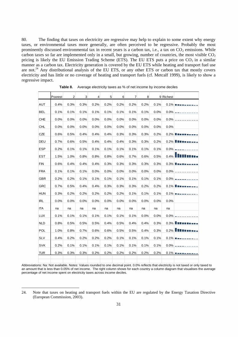
31

80. The finding that taxes on electricity are regressive may help to explain to some extent why energy

taxes, or environmental taxes more generally, are often perceived to be regressive. Probably the most

prominently discussed environmental tax in recent years is a carbon tax, i.e., a tax on CO2 emissions. While

carbon taxes so far are implemented only in a small, but growing, number of countries, the most visible CO2

pricing is likely the EU Emission Trading Scheme (ETS). The EU ETS puts a price on CO2 in a similar

manner as a carbon tax. Electricity generation is covered by the EU ETS while heating and transport fuel use

are not.24

Any distributional analysis of the EU ETS, or any other ETS or carbon tax that mostly covers

electricity and has little or no coverage of heating and transport fuels (cf. Metcalf 1999), is likely to show a

regressive impact.

Table 8. Average electricity taxes as % of net income by income deciles

Abbreviations: Na: Not available. Notes: Values rounded to one decimal point. 0.0% reflects that electricity is not taxed or only taxed to an amount that is less than 0.05% of net income. The right column shows for each country a column diagram that visualises the average percentage of net income spent on electricity taxes across income deciles.

24. Note that taxes on heating and transport fuels within the EU are regulated by the Energy Taxation Directive

(European Commission, 2003).

Poorest 2 3 4 5 6 7 8 9 Richest

AUT 0.4% 0.3% 0.3% 0.2% 0.2% 0.2% 0.2% 0.2% 0.1% 0.1%

BEL 0.1% 0.1% 0.1% 0.1% 0.1% 0.1% 0.1% 0.1% 0.0% 0.0%

CHE 0.0% 0.0% 0.0% 0.0% 0.0% 0.0% 0.0% 0.0% 0.0% 0.0%

CHL 0.0% 0.0% 0.0% 0.0% 0.0% 0.0% 0.0% 0.0% 0.0% 0.0%

CZE 0.6% 0.5% 0.4% 0.4% 0.4% 0.3% 0.3% 0.3% 0.2% 0.2%

DEU 0.7% 0.6% 0.5% 0.4% 0.4% 0.4% 0.3% 0.3% 0.2% 0.2%

ESP 0.2% 0.1% 0.1% 0.1% 0.1% 0.1% 0.1% 0.1% 0.1% 0.0%

EST 1.5% 1.0% 0.8% 0.8% 0.8% 0.6% 0.7% 0.6% 0.5% 0.4%

FIN 0.6% 0.4% 0.4% 0.4% 0.3% 0.3% 0.3% 0.3% 0.3% 0.3%

FRA 0.1% 0.1% 0.1% 0.0% 0.0% 0.0% 0.0% 0.0% 0.0% 0.0%

GBR 0.2% 0.2% 0.1% 0.1% 0.1% 0.1% 0.1% 0.1% 0.1% 0.0%

GRC 0.7% 0.5% 0.4% 0.4% 0.3% 0.3% 0.3% 0.2% 0.2% 0.1%

HUN 0.3% 0.2% 0.2% 0.2% 0.2% 0.2% 0.1% 0.1% 0.1% 0.1%

IRL 0.0% 0.0% 0.0% 0.0% 0.0% 0.0% 0.0% 0.0% 0.0% 0.0%

ITA na na na na na na na na na na

LUX 0.1% 0.1% 0.1% 0.1% 0.1% 0.1% 0.1% 0.0% 0.0% 0.0%

NLD 0.8% 0.5% 0.5% 0.5% 0.4% 0.5% 0.4% 0.4% 0.3% 0.3%

POL 1.0% 0.8% 0.7% 0.6% 0.6% 0.5% 0.5% 0.4% 0.3% 0.2%

SLV 0.4% 0.2% 0.2% 0.2% 0.2% 0.1% 0.1% 0.1% 0.1% 0.1%

SVK 0.2% 0.1% 0.1% 0.1% 0.1% 0.1% 0.1% 0.1% 0.1% 0.0%

TUR 0.3% 0.3% 0.3% 0.2% 0.2% 0.2% 0.2% 0.2% 0.2% 0.1%

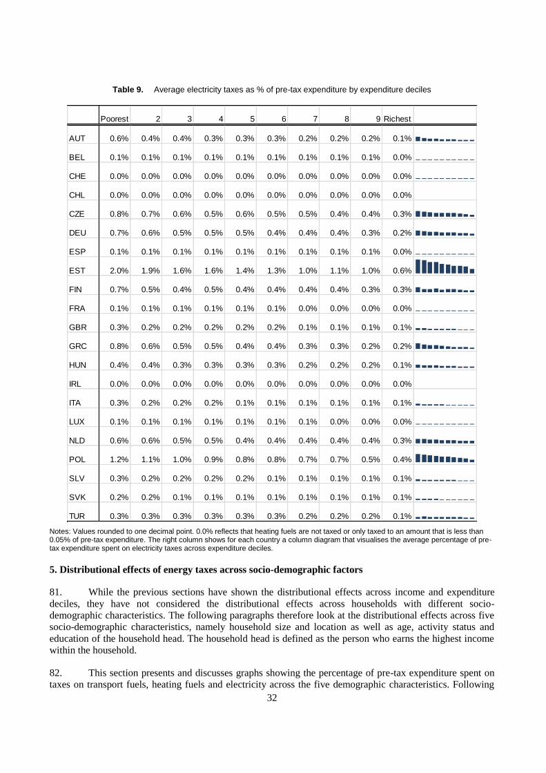
32

Table 9. Average electricity taxes as % of pre-tax expenditure by expenditure deciles

Notes: Values rounded to one decimal point. 0.0% reflects that heating fuels are not taxed or only taxed to an amount that is less than 0.05% of pre-tax expenditure. The right column shows for each country a column diagram that visualises the average percentage of pre-tax expenditure spent on electricity taxes across expenditure deciles.

5. Distributional effects of energy taxes across socio-demographic factors

81. While the previous sections have shown the distributional effects across income and expenditure

deciles, they have not considered the distributional effects across households with different socio-

demographic characteristics. The following paragraphs therefore look at the distributional effects across five

socio-demographic characteristics, namely household size and location as well as age, activity status and

education of the household head. The household head is defined as the person who earns the highest income

within the household.

82. This section presents and discusses graphs showing the percentage of pre-tax expenditure spent on

taxes on transport fuels, heating fuels and electricity across the five demographic characteristics. Following

Poorest 2 3 4 5 6 7 8 9 Richest

AUT 0.6% 0.4% 0.4% 0.3% 0.3% 0.3% 0.2% 0.2% 0.2% 0.1%

BEL 0.1% 0.1% 0.1% 0.1% 0.1% 0.1% 0.1% 0.1% 0.1% 0.0%

CHE 0.0% 0.0% 0.0% 0.0% 0.0% 0.0% 0.0% 0.0% 0.0% 0.0%

CHL 0.0% 0.0% 0.0% 0.0% 0.0% 0.0% 0.0% 0.0% 0.0% 0.0%

CZE 0.8% 0.7% 0.6% 0.5% 0.6% 0.5% 0.5% 0.4% 0.4% 0.3%

DEU 0.7% 0.6% 0.5% 0.5% 0.5% 0.4% 0.4% 0.4% 0.3% 0.2%

ESP 0.1% 0.1% 0.1% 0.1% 0.1% 0.1% 0.1% 0.1% 0.1% 0.0%

EST 2.0% 1.9% 1.6% 1.6% 1.4% 1.3% 1.0% 1.1% 1.0% 0.6%

FIN 0.7% 0.5% 0.4% 0.5% 0.4% 0.4% 0.4% 0.4% 0.3% 0.3%

FRA 0.1% 0.1% 0.1% 0.1% 0.1% 0.1% 0.0% 0.0% 0.0% 0.0%

GBR 0.3% 0.2% 0.2% 0.2% 0.2% 0.2% 0.1% 0.1% 0.1% 0.1%

GRC 0.8% 0.6% 0.5% 0.5% 0.4% 0.4% 0.3% 0.3% 0.2% 0.2%

HUN 0.4% 0.4% 0.3% 0.3% 0.3% 0.3% 0.2% 0.2% 0.2% 0.1%

IRL 0.0% 0.0% 0.0% 0.0% 0.0% 0.0% 0.0% 0.0% 0.0% 0.0%

ITA 0.3% 0.2% 0.2% 0.2% 0.1% 0.1% 0.1% 0.1% 0.1% 0.1%

LUX 0.1% 0.1% 0.1% 0.1% 0.1% 0.1% 0.1% 0.0% 0.0% 0.0%

NLD 0.6% 0.6% 0.5% 0.5% 0.4% 0.4% 0.4% 0.4% 0.4% 0.3%

POL 1.2% 1.1% 1.0% 0.9% 0.8% 0.8% 0.7% 0.7% 0.5% 0.4%

SLV 0.3% 0.2% 0.2% 0.2% 0.2% 0.1% 0.1% 0.1% 0.1% 0.1%

SVK 0.2% 0.2% 0.1% 0.1% 0.1% 0.1% 0.1% 0.1% 0.1% 0.1%

TUR 0.3% 0.3% 0.3% 0.3% 0.3% 0.3% 0.2% 0.2% 0.2% 0.1%

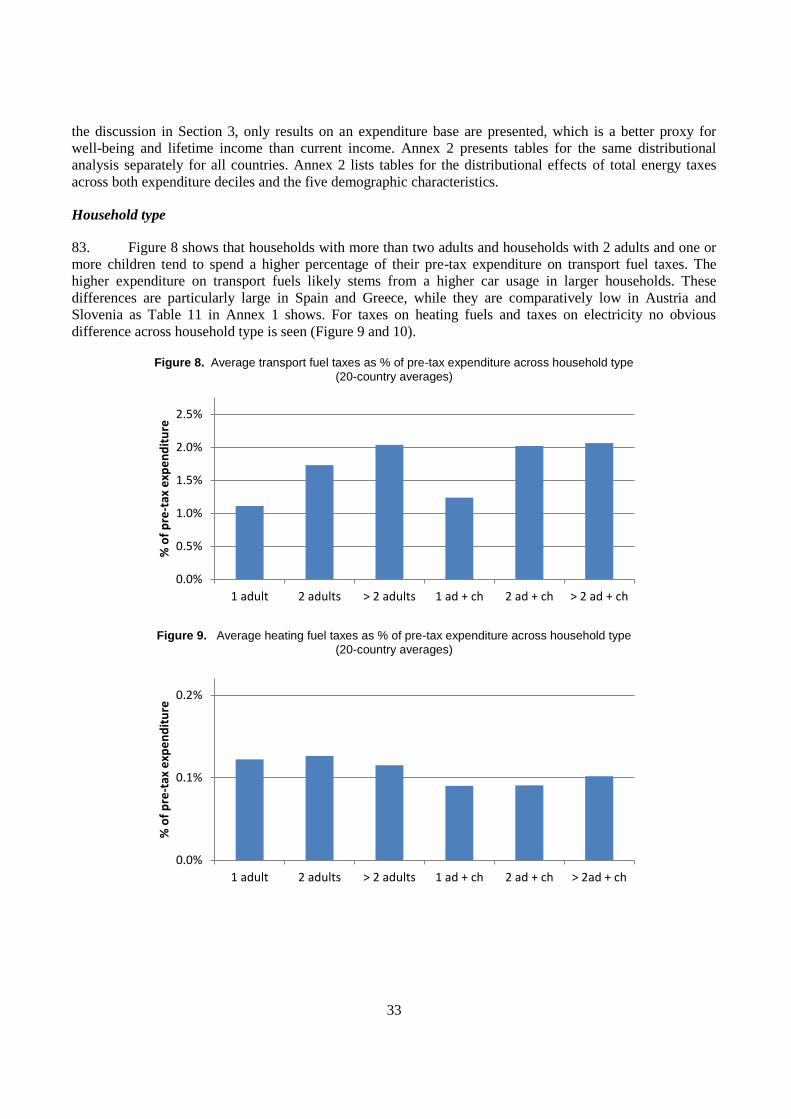
33

the discussion in Section 3, only results on an expenditure base are presented, which is a better proxy for

well-being and lifetime income than current income. Annex 2 presents tables for the same distributional

analysis separately for all countries. Annex 2 lists tables for the distributional effects of total energy taxes

across both expenditure deciles and the five demographic characteristics.

Household type

83. Figure 8 shows that households with more than two adults and households with 2 adults and one or

more children tend to spend a higher percentage of their pre-tax expenditure on transport fuel taxes. The

higher expenditure on transport fuels likely stems from a higher car usage in larger households. These

differences are particularly large in Spain and Greece, while they are comparatively low in Austria and

Slovenia as Table 11 in Annex 1 shows. For taxes on heating fuels and taxes on electricity no obvious

difference across household type is seen (Figure 9 and 10).

Figure 8. Average transport fuel taxes as % of pre-tax expenditure across household type

(20-country averages)

Figure 9. Average heating fuel taxes as % of pre-tax expenditure across household type

(20-country averages)

0.0%

0.5%

1.0%

1.5%

2.0%

2.5%

1 adult 2 adults > 2 adults 1 ad + ch 2 ad + ch > 2 ad + ch

% o

f p

re-t

ax e

xpe

nd

itu

re

0.0%

0.1%

0.2%

1 adult 2 adults > 2 adults 1 ad + ch 2 ad + ch > 2ad + ch

% o

f p

re-t

ax e

xpe

nd

itu

re

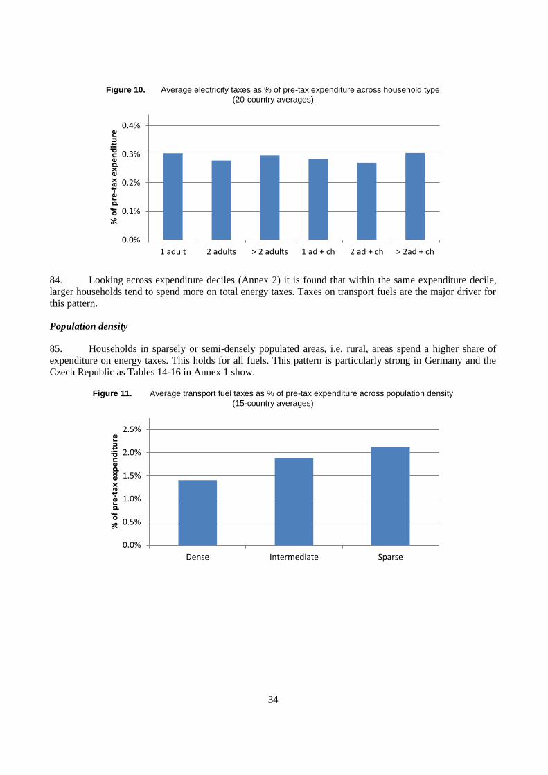
34

Figure 10. Average electricity taxes as % of pre-tax expenditure across household type

(20-country averages)

84. Looking across expenditure deciles (Annex 2) it is found that within the same expenditure decile,

larger households tend to spend more on total energy taxes. Taxes on transport fuels are the major driver for

this pattern.

Population density

85. Households in sparsely or semi-densely populated areas, i.e. rural, areas spend a higher share of

expenditure on energy taxes. This holds for all fuels. This pattern is particularly strong in Germany and the

Czech Republic as Tables 14-16 in Annex 1 show.

Figure 11. Average transport fuel taxes as % of pre-tax expenditure across population density

(15-country averages)

0.0%

0.1%

0.2%

0.3%

0.4%

1 adult 2 adults > 2 adults 1 ad + ch 2 ad + ch > 2ad + ch

% o

f p

re-t

ax e

xpe

nd

itu

re

0.0%

0.5%

1.0%

1.5%

2.0%

2.5%

Dense Intermediate Sparse

% o

f p

re-t

ax e

xpe

nd

itu

re

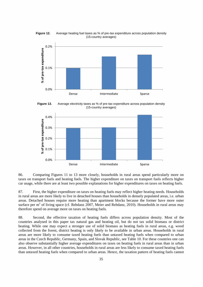
35

Figure 12. Average heating fuel taxes as % of pre-tax expenditure across population density

(15-country averages)

Figure 13. Average electricity taxes as % of pre-tax expenditure across population density

(15-country averages)

86. Comparing Figures 11 to 13 more closely, households in rural areas spend particularly more on

taxes on transport fuels and heating fuels. The higher expenditure on taxes on transport fuels reflects higher

car usage, while there are at least two possible explanations for higher expenditures on taxes on heating fuels.

87. First, the higher expenditure on taxes on heating fuels may reflect higher heating needs. Households

in rural areas are more likely to live in detached houses than households in densely populated areas, i.e. urban

areas. Detached houses require more heating than apartment blocks because the former have more outer

surface per m2 of living space (cf. Rehdanz 2007, Meier and Rehdanz, 2010). Households in rural areas may

therefore spend on average more on taxes on heating fuels.

88. Second, the effective taxation of heating fuels differs across population density. Most of the

countries analysed in this paper tax natural gas and heating oil, but do not tax solid biomass or district

heating. While one may expect a stronger use of solid biomass as heating fuels in rural areas, e.g. wood

collected from the forest, district heating is only likely to be available in urban areas. Households in rural

areas are more likely to consume taxed heating fuels than untaxed heating fuels when compared to urban

areas in the Czech Republic, Germany, Spain, and Slovak Republic, see Table 10. For these countries one can

also observe substantially higher average expenditures on taxes on heating fuels in rural areas than in urban

areas. However, in all other countries, households in rural areas are less likely to consume taxed heating fuels

than untaxed heating fuels when compared to urban areas. Hence, the taxation pattern of heating fuels cannot

0.0%

0.1%

0.2%

Dense Intermediate Sparse

% o

f p

re-t

ax e

xpe

nd

itu

re

0.0%

0.1%

0.2%

0.3%

0.4%

Dense Intermediate Sparse

% o

f p

re-t

ax e

xpe

nd

itu

re

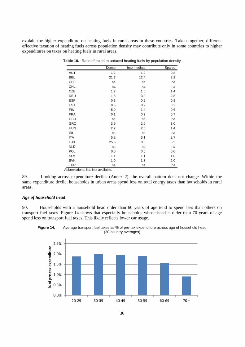
36

explain the higher expenditure on heating fuels in rural areas in these countries. Taken together, different

effective taxation of heating fuels across population density may contribute only in some countries to higher

expenditures on taxes on heating fuels in rural areas.

Table 10. Ratio of taxed to untaxed heating fuels by population density

Dense Intermediate Sparse

AUT 1.2 1.2 0.8

BEL 21.7 12.4 8.2

CHE na na na

CHL na na na

CZE 1.2 1.6 1.4

DEU 1.8 3.0 2.8

ESP 0.3 0.5 0.8

EST 0.5 0.2 0.2

FIN 5.9 1.4 0.6

FRA 0.1 0.2 0.7

GBR na na na

GRC 3.9 2.9 3.0

HUN 2.2 2.0 1.4

IRL na na na

ITA 5.2 5.1 2.7

LUX 25.5 8.3 5.5

NLD na na na

POL 0.0 0.0 0.0

SLV 1.1 1.1 1.0

SVK 1.0 1.8 2.0

TUR na na na

Abbreviations: Na: Not available.

89. Looking across expenditure deciles (Annex 2), the overall pattern does not change. Within the

same expenditure decile, households in urban areas spend less on total energy taxes than households in rural

areas.

Age of household head

90. Households with a household head older than 60 years of age tend to spend less than others on

transport fuel taxes. Figure 14 shows that especially households whose head is older than 70 years of age

spend less on transport fuel taxes. This likely reflects lower car usage.

Figure 14. Average transport fuel taxes as % of pre-tax expenditure across age of household head

(20-country averages)

0.0%

0.5%

1.0%

1.5%

2.0%

2.5%

20-29 30-39 40-49 50-59 60-69 70 +

% o

f p

re-t

ax e

xpe

nd

itu

re

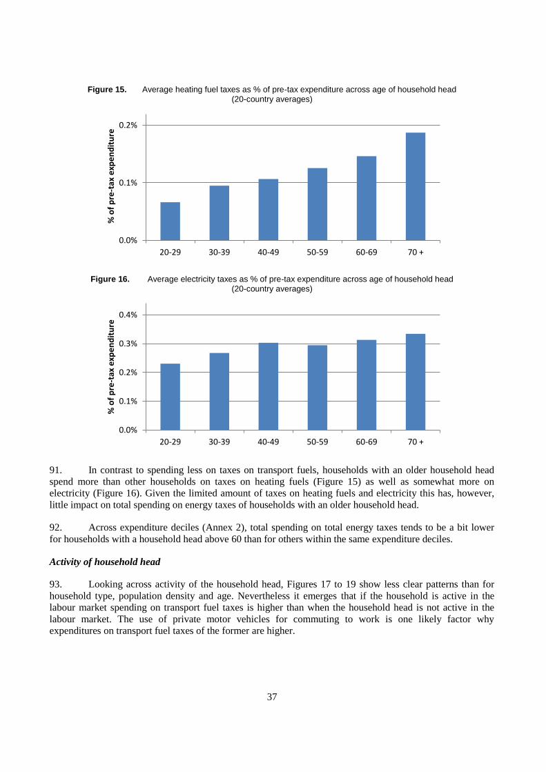
37

Figure 15. Average heating fuel taxes as % of pre-tax expenditure across age of household head

(20-country averages)

Figure 16. Average electricity taxes as % of pre-tax expenditure across age of household head

(20-country averages)

91. In contrast to spending less on taxes on transport fuels, households with an older household head

spend more than other households on taxes on heating fuels (Figure 15) as well as somewhat more on

electricity (Figure 16). Given the limited amount of taxes on heating fuels and electricity this has, however,

little impact on total spending on energy taxes of households with an older household head.

92. Across expenditure deciles (Annex 2), total spending on total energy taxes tends to be a bit lower

for households with a household head above 60 than for others within the same expenditure deciles.

Activity of household head

93. Looking across activity of the household head, Figures 17 to 19 show less clear patterns than for

household type, population density and age. Nevertheless it emerges that if the household is active in the

labour market spending on transport fuel taxes is higher than when the household head is not active in the

labour market. The use of private motor vehicles for commuting to work is one likely factor why

expenditures on transport fuel taxes of the former are higher.

0.0%

0.1%

0.2%

20-29 30-39 40-49 50-59 60-69 70 +

% o

f p

re-t

ax e

xpe

nd

itu

re

0.0%

0.1%

0.2%

0.3%

0.4%

20-29 30-39 40-49 50-59 60-69 70 +

% o

f p

re-t

ax e

xpe

nd

itu

re

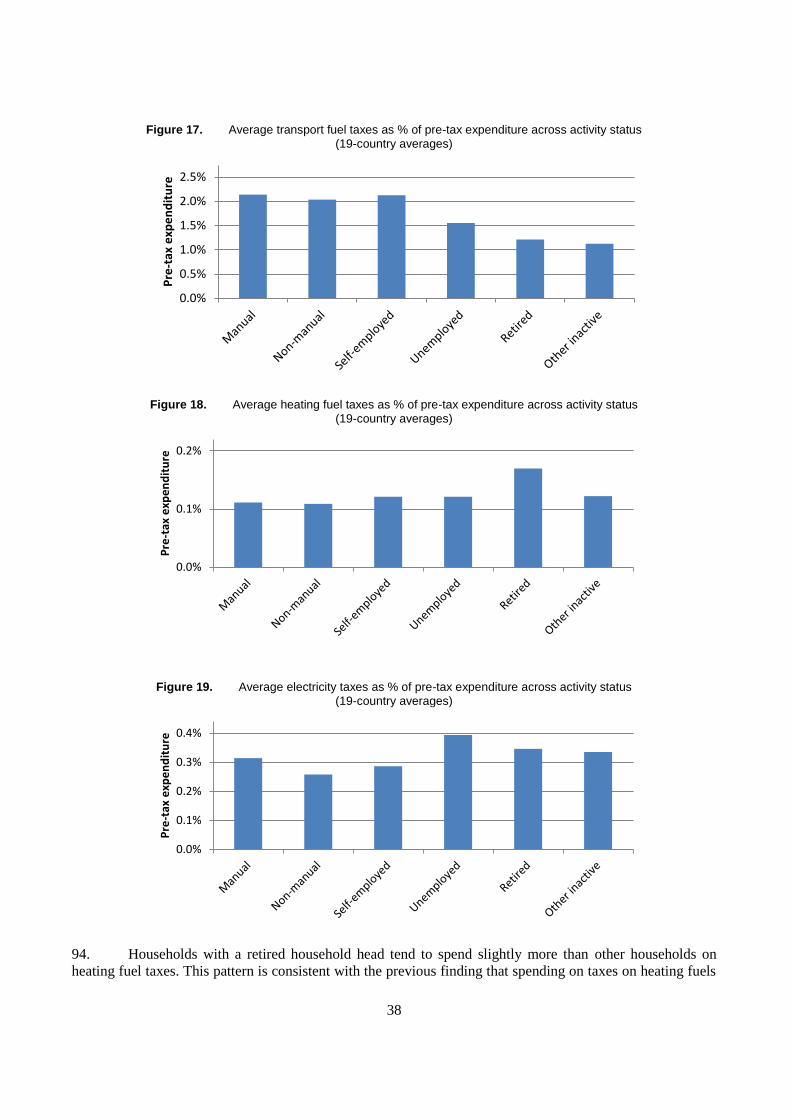
38

Figure 17. Average transport fuel taxes as % of pre-tax expenditure across activity status

(19-country averages)

Figure 18. Average heating fuel taxes as % of pre-tax expenditure across activity status

(19-country averages)

Figure 19. Average electricity taxes as % of pre-tax expenditure across activity status

(19-country averages)

94. Households with a retired household head tend to spend slightly more than other households on

heating fuel taxes. This pattern is consistent with the previous finding that spending on taxes on heating fuels

0.0%

0.5%

1.0%

1.5%

2.0%

2.5%P

re-t

ax e

xpe

nd

itu

re

0.0%

0.1%

0.2%

Pre

-tax

exp

en

dit

ure

0.0%

0.1%

0.2%

0.3%

0.4%

Pre

-tax

exp

en

dit

ure

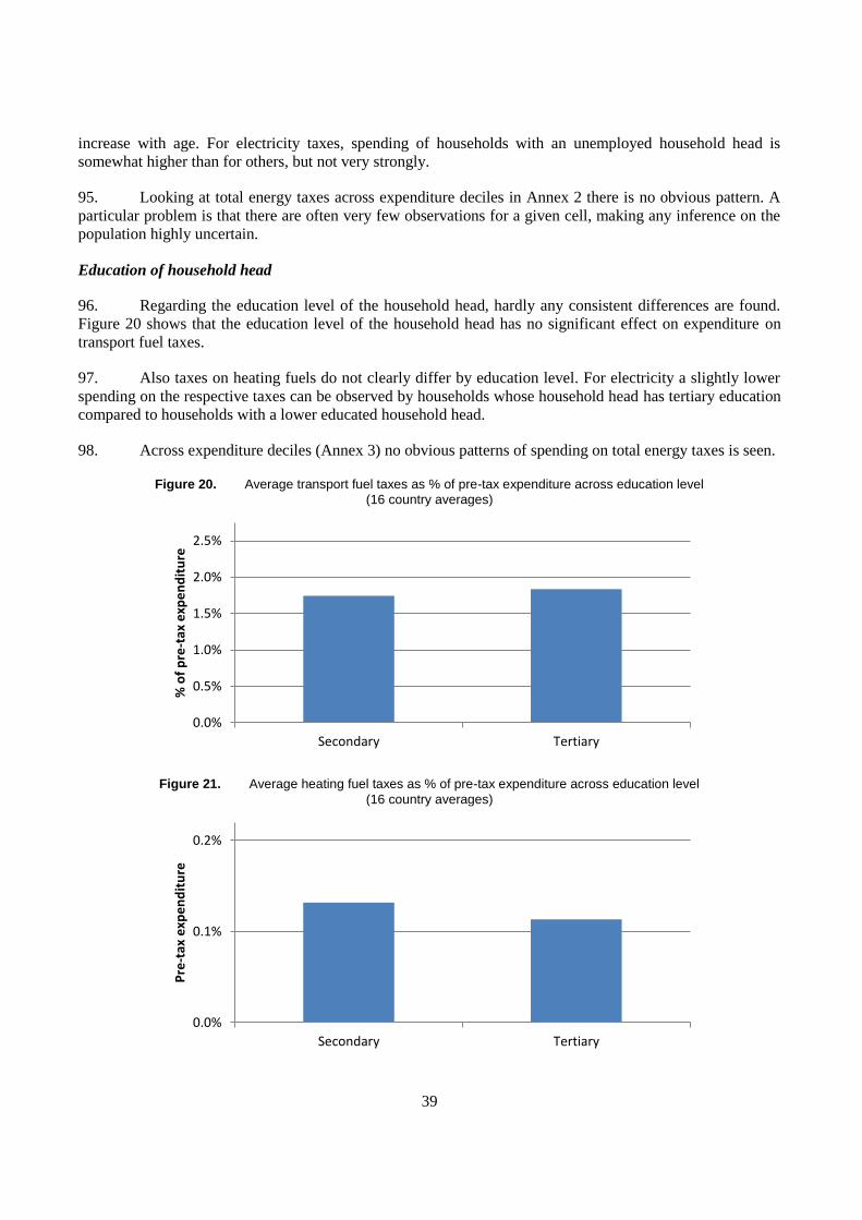
39

increase with age. For electricity taxes, spending of households with an unemployed household head is

somewhat higher than for others, but not very strongly.

95. Looking at total energy taxes across expenditure deciles in Annex 2 there is no obvious pattern. A

particular problem is that there are often very few observations for a given cell, making any inference on the

population highly uncertain.

Education of household head

96. Regarding the education level of the household head, hardly any consistent differences are found.

Figure 20 shows that the education level of the household head has no significant effect on expenditure on

transport fuel taxes.

97. Also taxes on heating fuels do not clearly differ by education level. For electricity a slightly lower

spending on the respective taxes can be observed by households whose household head has tertiary education

compared to households with a lower educated household head.

98. Across expenditure deciles (Annex 3) no obvious patterns of spending on total energy taxes is seen.

Figure 20. Average transport fuel taxes as % of pre-tax expenditure across education level

(16 country averages)

Figure 21. Average heating fuel taxes as % of pre-tax expenditure across education level

(16 country averages)

0.0%

0.5%

1.0%

1.5%

2.0%

2.5%

Secondary Tertiary

% o

f p

re-t

ax e

xpe

nd

itu

re

0.0%

0.1%

0.2%

Secondary Tertiary

Pre

-tax

exp

en

dit

ure

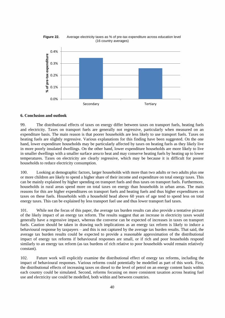
40

Figure 22. Average electricity taxes as % of pre-tax expenditure across education level

(16 country averages)

6. Conclusion and outlook

99. The distributional effects of taxes on energy differ between taxes on transport fuels, heating fuels

and electricity. Taxes on transport fuels are generally not regressive, particularly when measured on an

expenditure basis. The main reason is that poorer households are less likely to use transport fuels. Taxes on

heating fuels are slightly regressive. Various explanations for this finding have been suggested. On the one

hand, lower expenditure households may be particularly affected by taxes on heating fuels as they likely live

in more poorly insulated dwellings. On the other hand, lower expenditure households are more likely to live

in smaller dwellings with a smaller surface area to heat and may conserve heating fuels by heating up to lower

temperatures. Taxes on electricity are clearly regressive, which may be because it is difficult for poorer

households to reduce electricity consumption.

100. Looking at demographic factors, larger households with more than two adults or two adults plus one

or more children are likely to spend a higher share of their income and expenditure on total energy taxes. This

can be mainly explained by higher spending on transport fuels and thus taxes on transport fuels. Furthermore,

households in rural areas spend more on total taxes on energy than households in urban areas. The main

reasons for this are higher expenditures on transport fuels and heating fuels and thus higher expenditures on

taxes on these fuels. Households with a household head above 60 years of age tend to spend less on total

energy taxes. This can be explained by less transport fuel use and thus lower transport fuel taxes.

101. While not the focus of this paper, the average tax burden results can also provide a tentative picture

of the likely impact of an energy tax reform. The results suggest that an increase in electricity taxes would

generally have a regressive impact, whereas the converse can be expected of increases in taxes on transport

fuels. Caution should be taken in drawing such implications as an energy tax reform is likely to induce a

behavioural response by taxpayers – and this is not captured by the average tax burden results. That said, the

average tax burden results could be expected to provide a reasonable approximation of the distributional

impact of energy tax reforms if behavioural responses are small, or if rich and poor households respond

similarly to an energy tax reform (as tax burdens of rich relative to poor households would remain relatively

constant).

102. Future work will explicitly examine the distributional effect of energy tax reforms, including the

impact of behavioural responses. Various reforms could potentially be modelled as part of this work. First,

the distributional effects of increasing taxes on diesel to the level of petrol on an energy content basis within

each country could be simulated. Second, reforms focusing on more consistent taxation across heating fuel

use and electricity use could be modelled, both within and between countries.

0.0%

0.1%

0.2%

0.3%

0.4%

Secondary Tertiary

% o

f p

re-t

ax e

xpe

nd

itu

re

41

103. This analysis could also be extended to other environmentally related taxes and user fees, such as

taxes on motor vehicles or user fees for water, although this would require substantially more data. In the

former case, additional information would be needed on the type of car owned by households and in the latter

case the user fee schedules for households would need to be known.

104. Finally, future work could also incorporate a comparison of redistribution mechanisms that transfer

all or part of the tax revenue back to households. A possible focus could be on which mechanisms are

particular good at compensating the poor when increasing those energy taxes that are regressive. Another

potential question would be how much of the revenue is needed to compensate the poorest households fully.

REFERENCES

Baker, P., Blundell, R. and J. Micklewright (1989), “Modelling Household Energy Expenditures using Micro-

Data”, The Economic Journal, Vol. 99, No. 397, pp. 720-738.

Bozio, A., R. Dauvergne, B. Fabre, J. Goupille and O. Meslin (2012), Fiscalité et redistribution en France,

Institut des Politiques Publiques. Paris, France

Bundesministeriums für Verkehr, Bau und Stadtentwicklung, (2010), Transport in Germany 2008, Germany.

Bushnell, James B., Chong, H. and Erin T. Mansur (2013), "Profiting from Regulation: Evidence from the

European Carbon Market." American Economic Journal: Economic Policy, Vol. 5, No. 4, pp. 78-106.

Crozet, Yves (2009), The Prospects for Inter-Urban Travel Demand. OECD-ITF Discussion Paper.

Decoster, A., J Loughrey, C O'Donoghue and D. Verwerft (2010), “How regressive are indirect taxes?”,

Journal of Policy Analysis and Management, Vol. 29, No. 2, pp. 326-350.

Department for Transport (2011), National Travel Survey 2010, Department for Transport, United Kingdom.

Department for Transport (2013), Table ENV0103 (TSGB0303): Average new car fuel consumption: Great

Britain, 1997-2012, Department for Transport, United Kingdom

Destatis (2010), Energy consumption and CO2 emissions of road transport as part of the NAMEA

compilation strategy, Statistisches Bundesamt, Wiesbaden, Germany.

EEA (2011), EUA future prices 2005-2011, http://www.eea.europa.eu/data-and-maps/figures/eua-future-

prices-200520132011/eua-future-prices-200520132011-excel-file/at_download/file, Accessed on 21

January 2014.

Fabra, N. and Reguant, M. (2013), “Pass-through of emissions costs in electricity markets”, NBER Working

Paper 19613, National Bureau of Economic Research, Massachusetts.

European Commission (2013), “Part 2: Energy Products and Electricity” in Excise Duty tables, European

Commission, Brussels, Belgium.

European Commission (2011), Oil Bulletin, European Commission, Brussels, Belgium.

42

European Commission (2003), Council Directive 2003/96/EC of 27 October 2003 restructuring the

Community framework for the taxation of energy products and electricity, Official Journal, L 283, pp.

51-70.

Eurostat (2013), “Energy, transport and environment indicators”, Eurostat Pocket Books, Eurostat,

Luxembourg, Luxembourg.

Eurostat (2012), “Energy, transport and environment indicators”, Eurostat Pocket Books, Eurostat,

Luxembourg, Luxembourg.

Espey, M. (1998), “Gasoline demand revisited: an international meta-analysis of elasticities”, Energy

Economics, Vol. 20, No. 3, pp. 273-295.

Espey, J. and M. Espey (2004), “Turning on the lights: A meta-analysis of residential electricity demand

elasticities”, Journal of Agricultural and Applied Economics, Vol. 36, No. 1, pp. 65-81.

Goodwin, P. and Van Dender, K. (2013), “‘Peak Car’ — Themes and Issues”, Transport Reviews: A

Transnational Transdisciplinary Journal, Vol. 3, No. 3, pp. 243-254.

Harding, M. (2014a), “Personal Tax Treatment of Company Cars and Commuting Expenses: Estimating the

Fiscal and Environmental Costs”, OECD Taxation Working Paper, No. 20.

Harding, M. (2014b), “The Diesel Differential: Differences in the Tax Treatment of Gasoline and Diesel for

Road Use”, OECD Taxation Working Paper, No. 21.

Hurst, E., G. Li and B. Pugsley (2014), “Are Household Surveys Like Tax Forms: Evidence from Income

Underreporting of the Self Employed”, Review of Economics and Statistics, Vol. 96, No. 1, pp. 19-33..

IEA (2014a), “Extended world energy balances”, IEA World Energy Statistics and Balances (database). DOI:

10.1787/data-00513-en, Accessed on 20 February 2014.

IEA (2014b), “Emissions per kWh of electricity and heat output”, IEA CO2 Emissions from Fuel

Combustion Statistics (database). DOI: 10.1787/data-00432-en, Accessed on 21 January 2014.

IFS (2011), “Quantitative analysis of VAT rate structures” in IFS et al., “A retrospective evaluation of

elements of the EU VAT system”, Report prepared for the European Commission,

TAXUD/2010/DE/328.

IHS (2011), “The effect of VAT on price-setting behaviour” in IFS et al., “A retrospective evaluation of

elements of the EU VAT system”, Report prepared for the European Commission,

TAXUD/2010/DE/328.

Inspection générale des finances and Conseil général de l’économie, de l’industrie, de l’énergie et des

technologies (2012), Les prix, les marges et la consommation de carburants. Note de synthèse.

Krishnamurthy and Kriström, (2013), “Energy demand and income elasticity: a cross-country analysis”,

CERE Working Paper, 2013:5, Umea University, Sweden.

Leahy, E., S. Lyons and R. Tol (2011), “The distributional effects of value added tax in Ireland”, The

Economic and Social Review, Vol. 42, No. 2, pp. 213-235.

Meier, H. and K. Rehdanz (2010), “Determinants of residential space heating expenditures in Great Britain”

Energy Economics, Vol. 32, No.5, pp. 949-959.

43

Metcalf, G. E. (1999), “A distributional analysis of green tax reforms”, National Tax Journal, Vol. 52, No. 4,

pp. 655-682.

Ministerie van Verkeer en Waterstaat, (2005), Mobiliteitsonderzoek Nederland 2004, Ministerie van Verkeer

en Waterstaat , Netherlands.

OECD (2014a), “The Distributional Effects of Consumption Taxes in OECD countries”, OECD Tax Policy

Studies, No. 22, OECD, Paris, France.

OECD (2014b), OECD.Stat, (database). DOI: 10.1787/data-00285-en, Accessed on 23 September 2014

OECD (2013), Taxing Energy Use: A Graphical Analysis, OECD, Paris, France.

Poterba, J. M. (1991), “Is the gasoline tax regressive?”, Tax Policy and the Economy, Vol. 5, pp. 154-164.

Ravallion, M. (1992), “Poverty comparisons: A guide to concepts and methods” LSMS Working Paper, No

88, World Bank.

Rehdanz, K. (2007), “Determinants of residential space heating expenditures in Germany”, Energy

Economics, Vol. 29, No. 2, pp. 167-182.

Sijm, J., Neuhoff, K., Chen, Y. (2006), “CO2 cost pass-through and windfall profits in the power sector”,

Climate Policy, 6:1, 49-72.

SOeS - Inrets – Insee (2008), Enquête nationale transport et déplacements, 2008.

Sterner, T. (2012), “Distributional effects of taxing transport fuels”. Energy Policy, Vol. 41, pp. 75-83.

Verbruiksmonitor (2014), Average fuel consumption of cars build between 1994 and 2004, Autoweek.nl,

Sanoma Media Netherlands 2014: http://www.autoweek.nl/verbruiksmonitor, Accessed on 20 March

2014.

44

ANNEX I

Annex I provides tables showing the average tax burdens from energy taxes by country and by socio-

demographic factors. The main results of the distributional effect of energy taxes across socio-demographic

factors are discussed in Section 5. Whereas the focus of Section 5 is on comparing the distributional effect of

energy taxes across all 21 countries analysed Annex I lists the results separately by country.

Not all socio-demographic characteristics are available for all countries. Na abbreviates that data is not

available. Values are rounded to one decimal point. 0.0% reflects that the respective energy carriers are not

taxed or only taxed to an amount that is less than 0.05% of pre-tax expenditure.

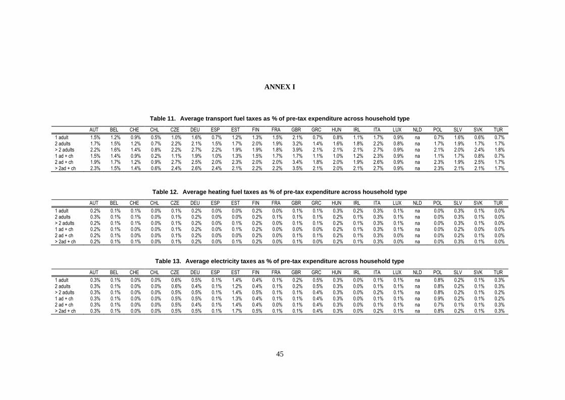
45

ANNEX I

Table 11. Average transport fuel taxes as % of pre-tax expenditure across household type

AUT BEL CHE CHL CZE DEU ESP EST FIN FRA GBR GRC HUN IRL ITA LUX NLD POL SLV SVK TUR

1 adult 1.5% 1.2% 0.9% 0.5% 1.0% 1.6% 0.7% 1.2% 1.3% 1.5% 2.1% 0.7% 0.8% 1.1% 1.7% 0.9% na 0.7% 1.6% 0.6% 0.7% 2 adults 1.7% 1.5% 1.2% 0.7% 2.2% 2.1% 1.5% 1.7% 2.0% 1.9% 3.2% 1.4% 1.6% 1.8% 2.2% 0.8% na 1.7% 1.9% 1.7% 1.7% > 2 adults 2.2% 1.6% 1.4% 0.8% 2.2% 2.7% 2.2% 1.9% 1.9% 1.8% 3.9% 2.1% 2.1% 2.1% 2.7% 0.9% na 2.1% 2.0% 2.4% 1.8% 1 ad + ch 1.5% 1.4% 0.9% 0.2% 1.1% 1.9% 1.0% 1.3% 1.5% 1.7% 1.7% 1.1% 1.0% 1.2% 2.3% 0.9% na 1.1% 1.7% 0.8% 0.7% 2 ad + ch 1.9% 1.7% 1.2% 0.9% 2.7% 2.5% 2.0% 2.3% 2.0% 2.0% 3.4% 1.8% 2.0% 1.9% 2.6% 0.9% na 2.3% 1.9% 2.5% 1.7% > 2ad + ch 2.3% 1.5% 1.4% 0.6% 2.4% 2.6% 2.4% 2.1% 2.2% 2.2% 3.5% 2.1% 2.0% 2.1% 2.7% 0.9% na 2.3% 2.1% 2.1% 1.7%

Table 12. Average heating fuel taxes as % of pre-tax expenditure across household type

AUT BEL CHE CHL CZE DEU ESP EST FIN FRA GBR GRC HUN IRL ITA LUX NLD POL SLV SVK TUR

1 adult 0.2% 0.1% 0.1% 0.0% 0.1% 0.2% 0.0% 0.0% 0.2% 0.0% 0.1% 0.1% 0.3% 0.2% 0.3% 0.1% na 0.0% 0.3% 0.1% 0.0% 2 adults 0.3% 0.1% 0.1% 0.0% 0.1% 0.2% 0.0% 0.0% 0.2% 0.1% 0.1% 0.1% 0.2% 0.1% 0.3% 0.1% na 0.0% 0.3% 0.1% 0.0% > 2 adults 0.2% 0.1% 0.1% 0.0% 0.1% 0.2% 0.0% 0.1% 0.2% 0.0% 0.1% 0.1% 0.2% 0.1% 0.3% 0.1% na 0.0% 0.3% 0.1% 0.0% 1 ad + ch 0.2% 0.1% 0.0% 0.0% 0.1% 0.2% 0.0% 0.1% 0.2% 0.0% 0.0% 0.0% 0.2% 0.1% 0.3% 0.1% na 0.0% 0.2% 0.0% 0.0% 2 ad + ch 0.2% 0.1% 0.0% 0.0% 0.1% 0.2% 0.0% 0.0% 0.2% 0.0% 0.1% 0.1% 0.2% 0.1% 0.3% 0.0% na 0.0% 0.2% 0.1% 0.0% > 2ad + ch 0.2% 0.1% 0.1% 0.0% 0.1% 0.2% 0.0% 0.1% 0.2% 0.0% 0.1% 0.0% 0.2% 0.1% 0.3% 0.0% na 0.0% 0.3% 0.1% 0.0%

Table 13. Average electricity taxes as % of pre-tax expenditure across household type

AUT BEL CHE CHL CZE DEU ESP EST FIN FRA GBR GRC HUN IRL ITA LUX NLD POL SLV SVK TUR

1 adult 0.3% 0.1% 0.0% 0.0% 0.6% 0.5% 0.1% 1.4% 0.4% 0.1% 0.2% 0.5% 0.3% 0.0% 0.1% 0.1% na 0.8% 0.2% 0.1% 0.3% 2 adults 0.3% 0.1% 0.0% 0.0% 0.6% 0.4% 0.1% 1.2% 0.4% 0.1% 0.2% 0.5% 0.3% 0.0% 0.1% 0.1% na 0.8% 0.2% 0.1% 0.3% > 2 adults 0.3% 0.1% 0.0% 0.0% 0.5% 0.5% 0.1% 1.4% 0.5% 0.1% 0.1% 0.4% 0.3% 0.0% 0.2% 0.1% na 0.8% 0.2% 0.1% 0.2% 1 ad + ch 0.3% 0.1% 0.0% 0.0% 0.5% 0.5% 0.1% 1.3% 0.4% 0.1% 0.1% 0.4% 0.3% 0.0% 0.1% 0.1% na 0.9% 0.2% 0.1% 0.2% 2 ad + ch 0.3% 0.1% 0.0% 0.0% 0.5% 0.4% 0.1% 1.4% 0.4% 0.0% 0.1% 0.4% 0.3% 0.0% 0.1% 0.1% na 0.7% 0.1% 0.1% 0.3% > 2ad + ch 0.3% 0.1% 0.0% 0.0% 0.5% 0.5% 0.1% 1.7% 0.5% 0.1% 0.1% 0.4% 0.3% 0.0% 0.2% 0.1% na 0.8% 0.2% 0.1% 0.3%

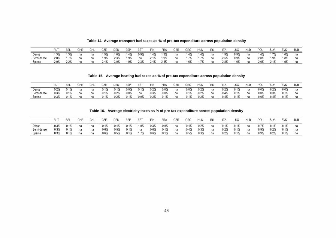
46

Table 14. Average transport fuel taxes as % of pre-tax expenditure across population density

AUT BEL CHE CHL CZE DEU ESP EST FIN FRA GBR GRC HUN IRL ITA LUX NLD POL SLV SVK TUR

Dense 1.3% 1.3% na na 1.5% 1.6% 1.4% 0.9% 1.4% 1.3% na 1.4% 1.4% na 1.9% 0.9% na 1.4% 1.7% 1.6% na Semi-dense 2.0% 1.7% na na 1.9% 2.3% 1.9% na 2.1% 1.9% na 1.7% 1.7% na 2.5% 0.9% na 2.0% 1.9% 1.8% na Sparse 2.0% 2.2% na na 2.4% 3.0% 1.9% 2.3% 2.4% 2.4% na 1.6% 1.7% na 2.8% 1.0% na 2.0% 2.1% 1.9% na

Table 15. Average heating fuel taxes as % of pre-tax expenditure across population density

AUT BEL CHE CHL CZE DEU ESP EST FIN FRA GBR GRC HUN IRL ITA LUX NLD POL SLV SVK TUR

Dense 0.2% 0.1% na na 0.1% 0.1% 0.0% 0.1% 0.2% 0.0% na 0.0% 0.2% na 0.2% 0.1% na 0.0% 0.2% 0.0% na Semi-dense 0.3% 0.1% na na 0.1% 0.2% 0.0% na 0.3% 0.0% na 0.1% 0.2% na 0.4% 0.1% na 0.0% 0.3% 0.1% na Sparse 0.3% 0.1% na na 0.1% 0.2% 0.1% 0.0% 0.2% 0.1% na 0.1% 0.2% na 0.4% 0.1% na 0.0% 0.4% 0.1% na

Table 16. Average electricity taxes as % of pre-tax expenditure across population density

AUT BEL CHE CHL CZE DEU ESP EST FIN FRA GBR GRC HUN IRL ITA LUX NLD POL SLV SVK TUR

Dense 0.3% 0.1% na na 0.4% 0.4% 0.1% 1.0% 0.3% 0.0% na 0.4% 0.2% na 0.1% 0.1% na 0.7% 0.1% 0.1% na Semi-dense 0.3% 0.1% na na 0.6% 0.5% 0.1% na 0.6% 0.1% na 0.4% 0.3% na 0.2% 0.1% na 0.9% 0.2% 0.1% na Sparse 0.3% 0.1% na na 0.6% 0.5% 0.1% 1.7% 0.6% 0.1% na 0.5% 0.3% na 0.2% 0.1% na 0.9% 0.2% 0.1% na

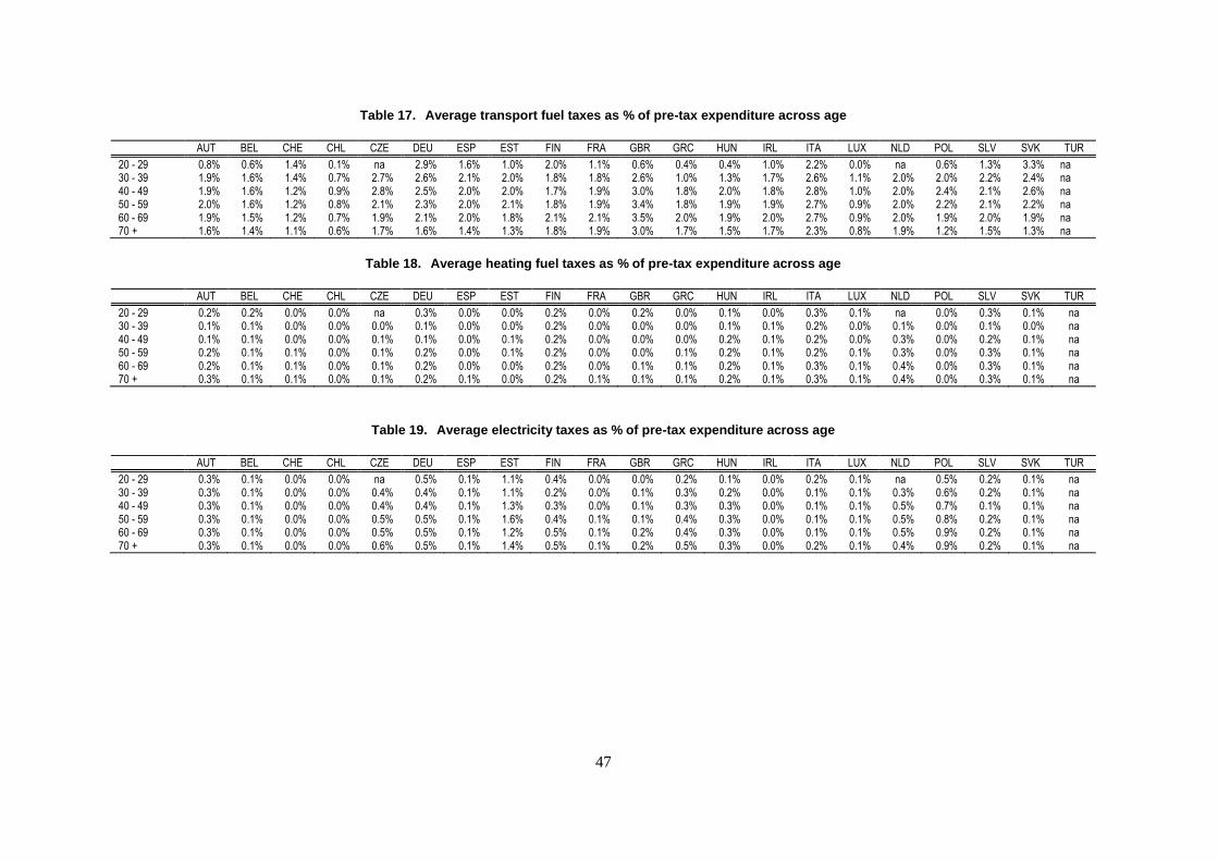
47

Table 17. Average transport fuel taxes as % of pre-tax expenditure across age

AUT BEL CHE CHL CZE DEU ESP EST FIN FRA GBR GRC HUN IRL ITA LUX NLD POL SLV SVK TUR

20 - 29 0.8% 0.6% 1.4% 0.1% na 2.9% 1.6% 1.0% 2.0% 1.1% 0.6% 0.4% 0.4% 1.0% 2.2% 0.0% na 0.6% 1.3% 3.3% na 30 - 39 1.9% 1.6% 1.4% 0.7% 2.7% 2.6% 2.1% 2.0% 1.8% 1.8% 2.6% 1.0% 1.3% 1.7% 2.6% 1.1% 2.0% 2.0% 2.2% 2.4% na 40 - 49 1.9% 1.6% 1.2% 0.9% 2.8% 2.5% 2.0% 2.0% 1.7% 1.9% 3.0% 1.8% 2.0% 1.8% 2.8% 1.0% 2.0% 2.4% 2.1% 2.6% na 50 - 59 2.0% 1.6% 1.2% 0.8% 2.1% 2.3% 2.0% 2.1% 1.8% 1.9% 3.4% 1.8% 1.9% 1.9% 2.7% 0.9% 2.0% 2.2% 2.1% 2.2% na 60 - 69 1.9% 1.5% 1.2% 0.7% 1.9% 2.1% 2.0% 1.8% 2.1% 2.1% 3.5% 2.0% 1.9% 2.0% 2.7% 0.9% 2.0% 1.9% 2.0% 1.9% na 70 + 1.6% 1.4% 1.1% 0.6% 1.7% 1.6% 1.4% 1.3% 1.8% 1.9% 3.0% 1.7% 1.5% 1.7% 2.3% 0.8% 1.9% 1.2% 1.5% 1.3% na

Table 18. Average heating fuel taxes as % of pre-tax expenditure across age

AUT BEL CHE CHL CZE DEU ESP EST FIN FRA GBR GRC HUN IRL ITA LUX NLD POL SLV SVK TUR

20 - 29 0.2% 0.2% 0.0% 0.0% na 0.3% 0.0% 0.0% 0.2% 0.0% 0.2% 0.0% 0.1% 0.0% 0.3% 0.1% na 0.0% 0.3% 0.1% na 30 - 39 0.1% 0.1% 0.0% 0.0% 0.0% 0.1% 0.0% 0.0% 0.2% 0.0% 0.0% 0.0% 0.1% 0.1% 0.2% 0.0% 0.1% 0.0% 0.1% 0.0% na 40 - 49 0.1% 0.1% 0.0% 0.0% 0.1% 0.1% 0.0% 0.1% 0.2% 0.0% 0.0% 0.0% 0.2% 0.1% 0.2% 0.0% 0.3% 0.0% 0.2% 0.1% na 50 - 59 0.2% 0.1% 0.1% 0.0% 0.1% 0.2% 0.0% 0.1% 0.2% 0.0% 0.0% 0.1% 0.2% 0.1% 0.2% 0.1% 0.3% 0.0% 0.3% 0.1% na 60 - 69 0.2% 0.1% 0.1% 0.0% 0.1% 0.2% 0.0% 0.0% 0.2% 0.0% 0.1% 0.1% 0.2% 0.1% 0.3% 0.1% 0.4% 0.0% 0.3% 0.1% na 70 + 0.3% 0.1% 0.1% 0.0% 0.1% 0.2% 0.1% 0.0% 0.2% 0.1% 0.1% 0.1% 0.2% 0.1% 0.3% 0.1% 0.4% 0.0% 0.3% 0.1% na

Table 19. Average electricity taxes as % of pre-tax expenditure across age

AUT BEL CHE CHL CZE DEU ESP EST FIN FRA GBR GRC HUN IRL ITA LUX NLD POL SLV SVK TUR

20 - 29 0.3% 0.1% 0.0% 0.0% na 0.5% 0.1% 1.1% 0.4% 0.0% 0.0% 0.2% 0.1% 0.0% 0.2% 0.1% na 0.5% 0.2% 0.1% na 30 - 39 0.3% 0.1% 0.0% 0.0% 0.4% 0.4% 0.1% 1.1% 0.2% 0.0% 0.1% 0.3% 0.2% 0.0% 0.1% 0.1% 0.3% 0.6% 0.2% 0.1% na 40 - 49 0.3% 0.1% 0.0% 0.0% 0.4% 0.4% 0.1% 1.3% 0.3% 0.0% 0.1% 0.3% 0.3% 0.0% 0.1% 0.1% 0.5% 0.7% 0.1% 0.1% na 50 - 59 0.3% 0.1% 0.0% 0.0% 0.5% 0.5% 0.1% 1.6% 0.4% 0.1% 0.1% 0.4% 0.3% 0.0% 0.1% 0.1% 0.5% 0.8% 0.2% 0.1% na 60 - 69 0.3% 0.1% 0.0% 0.0% 0.5% 0.5% 0.1% 1.2% 0.5% 0.1% 0.2% 0.4% 0.3% 0.0% 0.1% 0.1% 0.5% 0.9% 0.2% 0.1% na 70 + 0.3% 0.1% 0.0% 0.0% 0.6% 0.5% 0.1% 1.4% 0.5% 0.1% 0.2% 0.5% 0.3% 0.0% 0.2% 0.1% 0.4% 0.9% 0.2% 0.1% na

48

Table 20. Average transport fuel taxes as % of pre-tax expenditure across activity status

AUT BEL CHE CHL CZE DEU ESP EST FIN FRA GBR GRC HUN IRL ITA LUX NLD POL SLV SVK TUR

manual 2.3% 1.7% 1.2% na 2.5% 2.9% 2.1% 2.0% 2.3% 2.2% 3.4% 1.6% 1.8% 2.1% 2.9% 1.0% 2.3% 2.1% 2.0% 2.2% na non-manual 1.9% 1.7% 1.2% na 2.1% 2.4% 1.8% 1.9% 2.0% 1.9% 3.4% 2.0% 2.1% 1.8% 2.6% 1.0% 2.2% 2.2% 2.1% 2.3% na self-employed 2.1% 1.7% 1.2% na 2.7% 2.0% 2.2% 1.9% 1.7% 1.9% 3.7% 2.0% 2.6% 2.0% 2.7% 1.0% 1.7% 2.6% 1.8% 2.9% na unemployed 1.6% 1.3% 1.2% na 1.3% 1.3% 1.8% 2.5% 1.5% 1.8% 1.9% 1.5% 0.7% 1.9% 2.6% 0.8% 1.5% 0.7% 2.8% 0.7% na retired 1.2% 1.2% 0.8% na 1.2% 1.3% 1.0% 1.0% 1.2% 1.4% 2.1% 1.3% 1.0% 1.4% 1.7% 0.7% 1.4% 0.8% 1.3% 0.8% na other inactive 1.1% 1.4% 1.2% na 1.4% 1.2% 0.7% 1.2% 1.1% 1.2% na 0.7% 0.9% 1.3% 1.5% 0.8% 1.2% 0.6% 1.7% 1.0% na

Notes: In Belgium and Luxembourg no distinction is possible between manually employed, non-manually employed and self-employed. In Switzerland and the United Kingdom no distinction is possible between manually employed and non-manually employed. Furthermore, for Switzerland there is also no distinction possible between unemployed and other inactive.

Table 20. Average heating fuel taxes as % of pre-tax expenditure across activity status

AUT BEL CHE CHL CZE DEU ESP EST FIN FRA GBR GRC HUN IRL ITA LUX NLD POL SLV SVK TUR

manual 0.2% 0.1% 0.0% na 0.1% 0.2% 0.0% 0.0% 0.2% 0.0% 0.1% 0.0% 0.2% 0.1% 0.3% 0.0% 0.3% 0.0% 0.2% 0.1% na non-manual 0.2% 0.1% 0.0% na 0.1% 0.1% 0.0% 0.1% 0.2% 0.0% 0.1% 0.0% 0.2% 0.1% 0.2% 0.0% 0.3% 0.0% 0.3% 0.1% na self-employed 0.2% 0.1% 0.1% na 0.1% 0.2% 0.1% 0.0% 0.2% 0.1% 0.0% 0.1% 0.2% 0.1% 0.3% 0.0% 0.4% 0.0% 0.2% 0.1% na unemployed 0.2% 0.1% 0.1% na 0.1% 0.2% 0.0% 0.0% 0.2% 0.0% 0.1% 0.1% 0.2% 0.1% 0.3% 0.1% 0.5% 0.0% 0.2% 0.1% na retired 0.3% 0.1% 0.1% na 0.1% 0.2% 0.1% 0.0% 0.3% 0.1% 0.0% 0.1% 0.3% 0.1% 0.4% 0.1% 0.4% 0.0% 0.4% 0.1% na other inactive 0.1% 0.1% 0.1% na 0.1% 0.1% 0.1% 0.1% 0.2% 0.0% na 0.1% 0.2% 0.1% 0.3% 0.1% 0.3% 0.0% 0.2% 0.1% na

Notes: In Belgium and Luxembourg no distinction is possible between manually employed, non-manually employed and self-employed. In Switzerland and the United Kingdom no distinction is possible between manually employed and non-manually employed. Furthermore, for Switzerland there is also no distinction possible between unemployed and other inactive.

Table 21. Average electricity taxes as % of pre-tax expenditure across activity status

AUT BEL CHE CHL CZE DEU ESP EST FIN FRA GBR GRC HUN IRL ITA LUX NLD POL SLV SVK TUR

manual 0.3% 0.1% 0.0% na 0.5% 0.5% 0.1% 1.4% 0.4% 0.1% 0.1% 0.4% 0.3% 0.0% 0.1% 0.1% 0.5% 0.8% 0.2% 0.1% na non-manual 0.2% 0.1% 0.0% na 0.4% 0.4% 0.1% 1.2% 0.3% 0.0% 0.1% 0.3% 0.2% 0.0% 0.1% 0.1% 0.4% 0.6% 0.1% 0.1% na self-employed 0.3% 0.1% 0.0% na 0.5% 0.4% 0.1% 0.8% 0.5% 0.1% 0.2% 0.4% 0.3% 0.0% 0.1% 0.1% 0.5% 0.8% 0.2% 0.1% na unemployed 0.4% 0.1% 0.0% na 0.7% 0.7% 0.1% 1.5% 0.4% 0.1% 0.1% 0.5% 0.4% 0.0% 0.2% 0.1% 0.8% 1.1% 0.2% 0.2% na retired 0.4% 0.1% 0.0% na 0.6% 0.5% 0.1% 1.5% 0.6% 0.1% 0.2% 0.5% 0.3% 0.0% 0.2% 0.1% 0.4% 0.9% 0.2% 0.1% na other inactive 0.3% 0.1% 0.0% na 0.6% 0.5% 0.1% 1.6% 0.2% 0.1% na 0.5% 0.3% 0.0% 0.2% 0.1% 0.5% 0.7% 0.2% 0.2% na

Notes: In Belgium and Luxembourg no distinction is possible between manually employed, non-manually employed and self-employed. In Switzerland and the United Kingdom no distinction is possible between manually employed and non-manually employed. Furthermore, for Switzerland there is also no distinction possible between unemployed and other inactive.

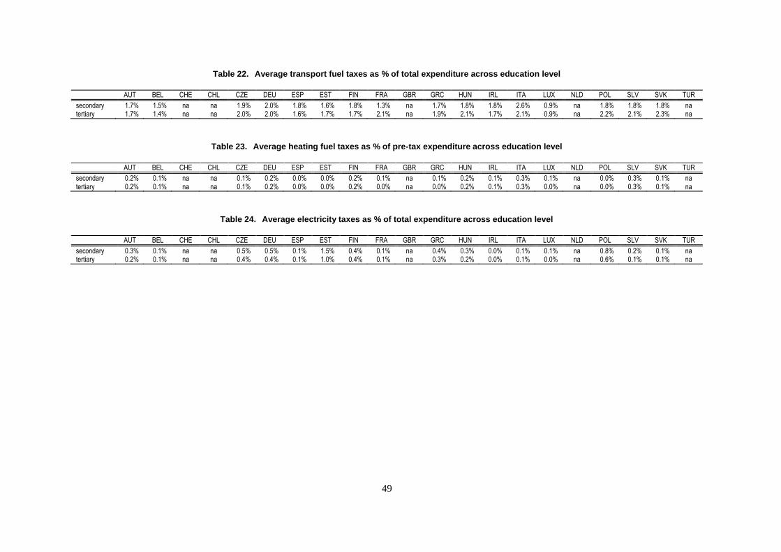
49

Table 22. Average transport fuel taxes as % of total expenditure across education level

AUT BEL CHE CHL CZE DEU ESP EST FIN FRA GBR GRC HUN IRL ITA LUX NLD POL SLV SVK TUR

secondary 1.7% 1.5% na na 1.9% 2.0% 1.8% 1.6% 1.8% 1.3% na 1.7% 1.8% 1.8% 2.6% 0.9% na 1.8% 1.8% 1.8% na tertiary 1.7% 1.4% na na 2.0% 2.0% 1.6% 1.7% 1.7% 2.1% na 1.9% 2.1% 1.7% 2.1% 0.9% na 2.2% 2.1% 2.3% na

Table 23. Average heating fuel taxes as % of pre-tax expenditure across education level

AUT BEL CHE CHL CZE DEU ESP EST FIN FRA GBR GRC HUN IRL ITA LUX NLD POL SLV SVK TUR

secondary 0.2% 0.1% na na 0.1% 0.2% 0.0% 0.0% 0.2% 0.1% na 0.1% 0.2% 0.1% 0.3% 0.1% na 0.0% 0.3% 0.1% na tertiary 0.2% 0.1% na na 0.1% 0.2% 0.0% 0.0% 0.2% 0.0% na 0.0% 0.2% 0.1% 0.3% 0.0% na 0.0% 0.3% 0.1% na

Table 24. Average electricity taxes as % of total expenditure across education level

AUT BEL CHE CHL CZE DEU ESP EST FIN FRA GBR GRC HUN IRL ITA LUX NLD POL SLV SVK TUR

secondary 0.3% 0.1% na na 0.5% 0.5% 0.1% 1.5% 0.4% 0.1% na 0.4% 0.3% 0.0% 0.1% 0.1% na 0.8% 0.2% 0.1% na tertiary 0.2% 0.1% na na 0.4% 0.4% 0.1% 1.0% 0.4% 0.1% na 0.3% 0.2% 0.0% 0.1% 0.0% na 0.6% 0.1% 0.1% na

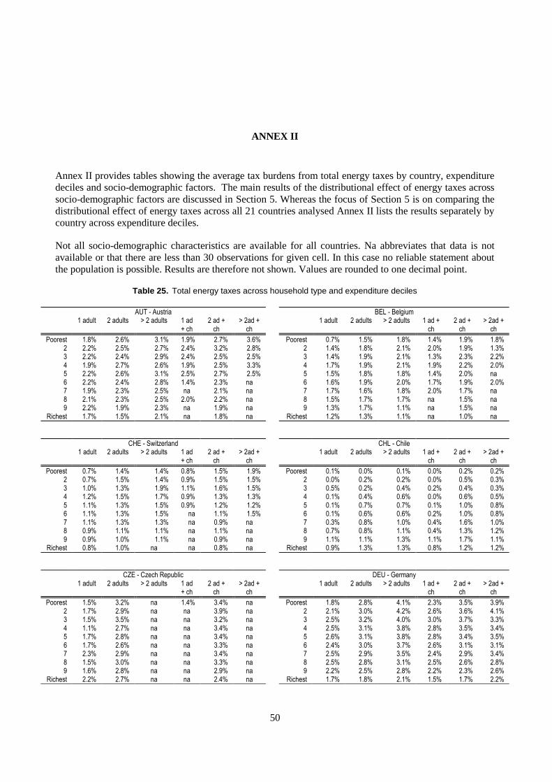
50

ANNEX II

Annex II provides tables showing the average tax burdens from total energy taxes by country, expenditure

deciles and socio-demographic factors. The main results of the distributional effect of energy taxes across

socio-demographic factors are discussed in Section 5. Whereas the focus of Section 5 is on comparing the

distributional effect of energy taxes across all 21 countries analysed Annex II lists the results separately by

country across expenditure deciles.

Not all socio-demographic characteristics are available for all countries. Na abbreviates that data is not

available or that there are less than 30 observations for given cell. In this case no reliable statement about

the population is possible. Results are therefore not shown. Values are rounded to one decimal point.

Table 25. Total energy taxes across household type and expenditure deciles

AUT - Austria BEL - Belgium 1 adult 2 adults > 2 adults 1 ad

+ ch 2 ad +

ch > 2ad +

ch 1 adult 2 adults > 2 adults 1 ad +

ch 2 ad +

ch > 2ad +

ch

Poorest 1.8% 2.6% 3.1% 1.9% 2.7% 3.6% Poorest 0.7% 1.5% 1.8% 1.4% 1.9% 1.8% 2 2.2% 2.5% 2.7% 2.4% 3.2% 2.8% 2 1.4% 1.8% 2.1% 2.0% 1.9% 1.3% 3 2.2% 2.4% 2.9% 2.4% 2.5% 2.5% 3 1.4% 1.9% 2.1% 1.3% 2.3% 2.2% 4 1.9% 2.7% 2.6% 1.9% 2.5% 3.3% 4 1.7% 1.9% 2.1% 1.9% 2.2% 2.0% 5 2.2% 2.6% 3.1% 2.5% 2.7% 2.5% 5 1.5% 1.8% 1.8% 1.4% 2.0% na 6 2.2% 2.4% 2.8% 1.4% 2.3% na 6 1.6% 1.9% 2.0% 1.7% 1.9% 2.0% 7 1.9% 2.3% 2.5% na 2.1% na 7 1.7% 1.6% 1.8% 2.0% 1.7% na 8 2.1% 2.3% 2.5% 2.0% 2.2% na 8 1.5% 1.7% 1.7% na 1.5% na 9 2.2% 1.9% 2.3% na 1.9% na 9 1.3% 1.7% 1.1% na 1.5% na

Richest 1.7% 1.5% 2.1% na 1.8% na Richest 1.2% 1.3% 1.1% na 1.0% na

CHE - Switzerland CHL - Chile 1 adult 2 adults > 2 adults 1 ad

+ ch 2 ad +

ch > 2ad +

ch 1 adult 2 adults > 2 adults 1 ad +

ch 2 ad +

ch > 2ad +

ch

Poorest 0.7% 1.4% 1.4% 0.8% 1.5% 1.9% Poorest 0.1% 0.0% 0.1% 0.0% 0.2% 0.2% 2 0.7% 1.5% 1.4% 0.9% 1.5% 1.5% 2 0.0% 0.2% 0.2% 0.0% 0.5% 0.3% 3 1.0% 1.3% 1.9% 1.1% 1.6% 1.5% 3 0.5% 0.2% 0.4% 0.2% 0.4% 0.3% 4 1.2% 1.5% 1.7% 0.9% 1.3% 1.3% 4 0.1% 0.4% 0.6% 0.0% 0.6% 0.5% 5 1.1% 1.3% 1.5% 0.9% 1.2% 1.2% 5 0.1% 0.7% 0.7% 0.1% 1.0% 0.8% 6 1.1% 1.3% 1.5% na 1.1% 1.5% 6 0.1% 0.6% 0.6% 0.2% 1.0% 0.8% 7 1.1% 1.3% 1.3% na 0.9% na 7 0.3% 0.8% 1.0% 0.4% 1.6% 1.0% 8 0.9% 1.1% 1.1% na 1.1% na 8 0.7% 0.8% 1.1% 0.4% 1.3% 1.2% 9 0.9% 1.0% 1.1% na 0.9% na 9 1.1% 1.1% 1.3% 1.1% 1.7% 1.1%

Richest 0.8% 1.0% na na 0.8% na Richest 0.9% 1.3% 1.3% 0.8% 1.2% 1.2%

CZE - Czech Republic DEU - Germany 1 adult 2 adults > 2 adults 1 ad

+ ch 2 ad +

ch > 2ad +

ch 1 adult 2 adults > 2 adults 1 ad +

ch 2 ad +

ch > 2ad +

ch

Poorest 1.5% 3.2% na 1.4% 3.4% na Poorest 1.8% 2.8% 4.1% 2.3% 3.5% 3.9% 2 1.7% 2.9% na na 3.9% na 2 2.1% 3.0% 4.2% 2.6% 3.6% 4.1% 3 1.5% 3.5% na na 3.2% na 3 2.5% 3.2% 4.0% 3.0% 3.7% 3.3% 4 1.1% 2.7% na na 3.4% na 4 2.5% 3.1% 3.8% 2.8% 3.5% 3.4% 5 1.7% 2.8% na na 3.4% na 5 2.6% 3.1% 3.8% 2.8% 3.4% 3.5% 6 1.7% 2.6% na na 3.3% na 6 2.4% 3.0% 3.7% 2.6% 3.1% 3.1% 7 2.3% 2.9% na na 3.4% na 7 2.5% 2.9% 3.5% 2.4% 2.9% 3.4% 8 1.5% 3.0% na na 3.3% na 8 2.5% 2.8% 3.1% 2.5% 2.6% 2.8% 9 1.6% 2.8% na na 2.9% na 9 2.2% 2.5% 2.8% 2.2% 2.3% 2.6%

Richest 2.2% 2.7% na na 2.4% na Richest 1.7% 1.8% 2.1% 1.5% 1.7% 2.2%

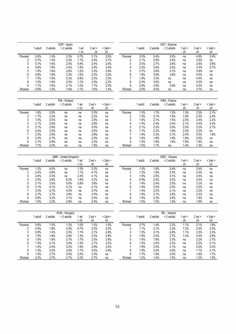
51

ESP - Spain EST - Estonia 1 adult 2 adults > 2 adults 1 ad

+ ch 2 ad +

ch > 2ad +

ch 1 adult 2 adults > 2 adults 1 ad +

ch 2 ad +

ch > 2ad +

ch

Poorest 0.6% 1.4% 2.3% 0.7% 2.1% 2.6% Poorest 3.5% 0.4% 3.9% na 4.8% 3.4% 2 0.7% 1.3% 2.4% 1.1% 2.4% 2.7% 2 2.1% 2.6% 2.4% na 3.9% na 3 0.7% 1.6% 2.5% 0.9% 2.4% 2.4% 3 3.5% 2.7% 2.6% na 2.6% 3.6% 4 0.6% 1.8% 2.4% 1.5% 2.4% 2.4% 4 2.2% 2.6% 2.5% na 3.3% 3.7% 5 1.0% 1.6% 2.6% 1.2% 2.3% 2.9% 5 2.7% 2.8% 3.1% na 3.9% na 6 0.8% 1.9% 2.3% 1.5% 2.2% 2.5% 6 1.8% 3.6% 3.9% na 4.0% na 7 1.0% 1.8% 2.2% 0.8% 2.2% 2.5% 7 1.8% 3.3% na na 4.4% na 8 1.0% 1.6% 2.5% 1.1% 2.0% 2.2% 8 2.4% 3.6% na na 4.2% na 9 1.1% 1.6% 2.1% 1.2% 1.7% 2.5% 9 2.8% 3.8% 2.9% na 4.3% na

Richest 0.8% 1.4% 1.6% 1.1% 1.6% 1.4% Richest 2.5% 3.5% na na 2.7% na

FIN - Finland FRA - France 1 adult 2 adults > 2 adults 1 ad

+ ch 2 ad +

ch > 2ad +

ch 1 adult 2 adults > 2 adults 1 ad +

ch 2 ad +

ch > 2ad +

ch

Poorest 1.8% 2.5% na na 2.5% na Poorest 1.3% 1.7% 1.3% 1.3% 2.3% 2.1% 2 1.7% 2.3% na na 2.2% na 2 1.5% 2.1% 1.6% 1.9% 2.5% 2.4% 3 1.5% 3.0% na na 2.5% na 3 1.6% 2.1% 1.5% 2.0% 2.4% 2.2% 4 2.1% 2.9% na na 2.8% na 4 1.4% 2.4% 2.4% 2.1% 2.4% 3.4% 5 2.1% 2.8% na na 3.0% na 5 2.1% 2.2% 3.0% 2.0% 2.2% 2.7% 6 2.4% 3.0% na na 2.6% na 6 1.7% 2.2% 1.8% 2.0% 2.2% na 7 2.3% 2.9% na na 2.8% na 7 1.9% 2.2% 2.1% 2.4% 2.0% 1.8% 8 2.0% 2.7% na na 2.5% na 8 1.6% 1.8% 1.9% 1.6% 2.0% na 9 2.1% 2.9% na na 2.2% na 9 1.5% 1.8% 1.9% 1.8% 1.8% na

Richest 1.7% 2.0% na na 1.9% na Richest 1.5% 1.7% na 1.4% 1.3% na

GBR - United Kingdom GRC - Greece 1 adult 2 adults > 2 adults 1 ad

+ ch 2 ad +

ch > 2ad +

ch 1 adult 2 adults > 2 adults 1 ad +

ch 2 ad +

ch > 2ad +

ch

Poorest 1.2% 4.0% na 1.3% 2.2% na Poorest 1.0% 1.6% 2.4% na 2.4% na 2 2.4% 3.6% na 1.1% 4.1% na 2 1.2% 1.8% 3.3% na 2.4% na 3 2.6% 4.3% na 2.3% 4.1% na 3 1.0% 2.5% 3.1% na 2.5% na 4 2.5% 3.6% 6.2% 1.9% 4.2% na 4 0.9% 2.0% 3.0% na 2.4% na 5 3.1% 3.5% 5.6% 2.8% 3.8% na 5 1.4% 2.4% 2.5% na 2.2% na 6 3.1% 4.1% 4.1% na 4.1% na 6 1.4% 2.0% 2.5% na 2.5% na 7 3.3% 3.7% 4.0% na 3.7% na 7 1.4% 2.2% 2.1% na 2.2% na 8 2.7% 3.7% 3.9% na 3.4% na 8 1.9% 2.1% 2.6% na 2.3% na 9 2.8% 3.2% 3.1% na 3.0% na 9 1.5% 2.2% 2.6% na 1.9% na

Richest 1.9% 2.2% 2.8% na 2.4% na Richest 1.5% 1.5% 1.8% na 1.8% na

HUN - Hungary IRL - Ireland 1 adult 2 adults > 2 adults 1 ad

+ ch 2 ad +

ch > 2ad +

ch 1 adult 2 adults > 2 adults 1 ad +

ch 2 ad +

ch > 2ad +

ch

Poorest 0.8% 1.0% 1.2% 1.0% 1.5% 1.5% Poorest 0.7% 1.4% 2.2% 1.1% 2.1% 1.8% 2 0.9% 1.8% 2.4% 0.7% 2.0% 2.5% 2 1.1% 2.1% 3.3% 1.2% 2.5% 2.4% 3 0.9% 1.4% 2.5% 1.1% 2.1% 2.8% 3 1.3% 2.1% 2.8% 1.1% 2.3% 2.3% 4 1.0% 1.8% 2.8% 1.3% 2.5% 2.8% 4 1.6% 2.0% 2.7% 1.4% 2.4% 2.6% 5 1.0% 1.9% 2.7% 1.7% 2.5% 2.9% 5 1.5% 1.9% 2.3% na 2.2% 2.7% 6 1.3% 2.1% 3.0% 1.3% 2.7% 3.2% 6 1.5% 2.4% 2.3% na 2.2% 2.1% 7 1.4% 2.4% 3.2% 1.9% 2.8% 3.5% 7 1.8% 2.0% 2.1% na 2.0% 2.0% 8 1.3% 2.5% 3.0% 1.7% 3.0% 2.6% 8 1.9% 2.0% 2.0% na 1.7% 2.1% 9 1.5% 2.7% 3.0% 2.2% 3.3% na 9 1.7% 1.8% 2.0% na 1.6% 1.7%

Richest 2.3% 2.7% 2.7% 2.2% 2.7% na Richest 1.2% 1.4% 1.5% na 1.2% 1.5%

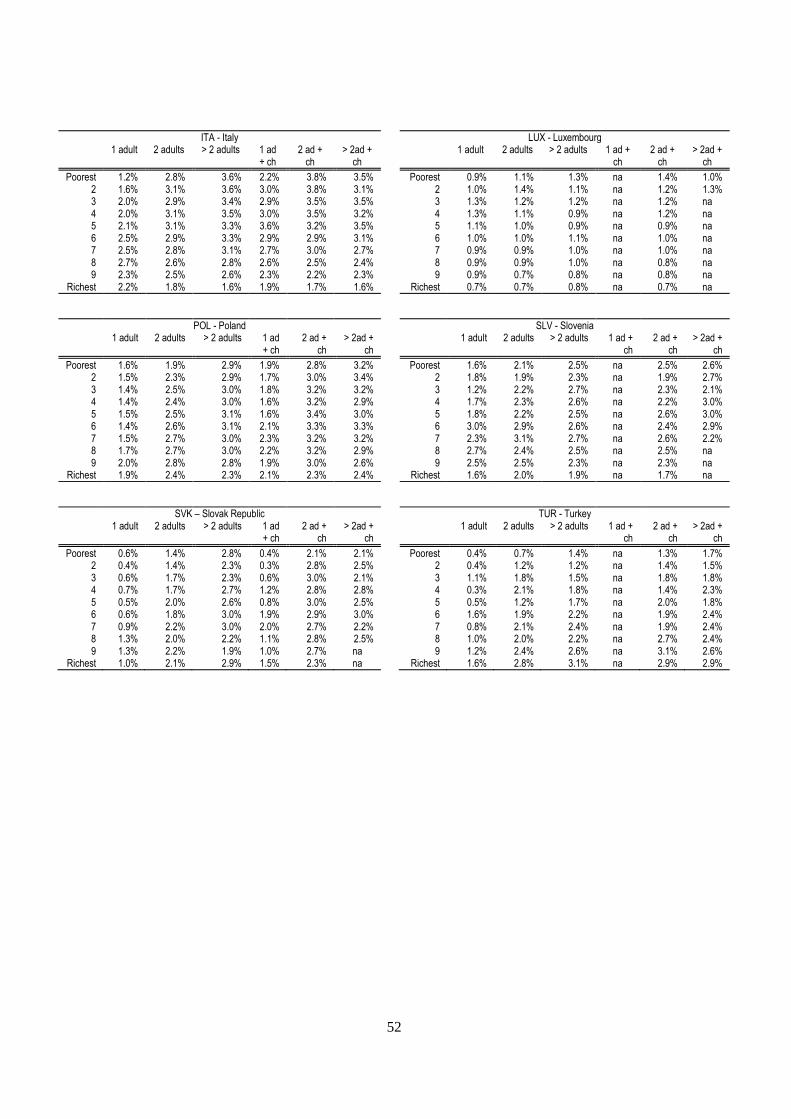
52

ITA - Italy LUX - Luxembourg 1 adult 2 adults > 2 adults 1 ad

+ ch 2 ad +

ch > 2ad +

ch 1 adult 2 adults > 2 adults 1 ad +

ch 2 ad +

ch > 2ad +

ch

Poorest 1.2% 2.8% 3.6% 2.2% 3.8% 3.5% Poorest 0.9% 1.1% 1.3% na 1.4% 1.0% 2 1.6% 3.1% 3.6% 3.0% 3.8% 3.1% 2 1.0% 1.4% 1.1% na 1.2% 1.3% 3 2.0% 2.9% 3.4% 2.9% 3.5% 3.5% 3 1.3% 1.2% 1.2% na 1.2% na 4 2.0% 3.1% 3.5% 3.0% 3.5% 3.2% 4 1.3% 1.1% 0.9% na 1.2% na 5 2.1% 3.1% 3.3% 3.6% 3.2% 3.5% 5 1.1% 1.0% 0.9% na 0.9% na 6 2.5% 2.9% 3.3% 2.9% 2.9% 3.1% 6 1.0% 1.0% 1.1% na 1.0% na 7 2.5% 2.8% 3.1% 2.7% 3.0% 2.7% 7 0.9% 0.9% 1.0% na 1.0% na 8 2.7% 2.6% 2.8% 2.6% 2.5% 2.4% 8 0.9% 0.9% 1.0% na 0.8% na 9 2.3% 2.5% 2.6% 2.3% 2.2% 2.3% 9 0.9% 0.7% 0.8% na 0.8% na

Richest 2.2% 1.8% 1.6% 1.9% 1.7% 1.6% Richest 0.7% 0.7% 0.8% na 0.7% na

POL - Poland SLV - Slovenia 1 adult 2 adults > 2 adults 1 ad

+ ch 2 ad +

ch > 2ad +

ch 1 adult 2 adults > 2 adults 1 ad +

ch 2 ad +

ch > 2ad +

ch

Poorest 1.6% 1.9% 2.9% 1.9% 2.8% 3.2% Poorest 1.6% 2.1% 2.5% na 2.5% 2.6% 2 1.5% 2.3% 2.9% 1.7% 3.0% 3.4% 2 1.8% 1.9% 2.3% na 1.9% 2.7% 3 1.4% 2.5% 3.0% 1.8% 3.2% 3.2% 3 1.2% 2.2% 2.7% na 2.3% 2.1% 4 1.4% 2.4% 3.0% 1.6% 3.2% 2.9% 4 1.7% 2.3% 2.6% na 2.2% 3.0% 5 1.5% 2.5% 3.1% 1.6% 3.4% 3.0% 5 1.8% 2.2% 2.5% na 2.6% 3.0% 6 1.4% 2.6% 3.1% 2.1% 3.3% 3.3% 6 3.0% 2.9% 2.6% na 2.4% 2.9% 7 1.5% 2.7% 3.0% 2.3% 3.2% 3.2% 7 2.3% 3.1% 2.7% na 2.6% 2.2% 8 1.7% 2.7% 3.0% 2.2% 3.2% 2.9% 8 2.7% 2.4% 2.5% na 2.5% na 9 2.0% 2.8% 2.8% 1.9% 3.0% 2.6% 9 2.5% 2.5% 2.3% na 2.3% na

Richest 1.9% 2.4% 2.3% 2.1% 2.3% 2.4% Richest 1.6% 2.0% 1.9% na 1.7% na

SVK – Slovak Republic TUR - Turkey 1 adult 2 adults > 2 adults 1 ad

+ ch 2 ad +

ch > 2ad +

ch 1 adult 2 adults > 2 adults 1 ad +

ch 2 ad +

ch > 2ad +

ch

Poorest 0.6% 1.4% 2.8% 0.4% 2.1% 2.1% Poorest 0.4% 0.7% 1.4% na 1.3% 1.7% 2 0.4% 1.4% 2.3% 0.3% 2.8% 2.5% 2 0.4% 1.2% 1.2% na 1.4% 1.5% 3 0.6% 1.7% 2.3% 0.6% 3.0% 2.1% 3 1.1% 1.8% 1.5% na 1.8% 1.8% 4 0.7% 1.7% 2.7% 1.2% 2.8% 2.8% 4 0.3% 2.1% 1.8% na 1.4% 2.3% 5 0.5% 2.0% 2.6% 0.8% 3.0% 2.5% 5 0.5% 1.2% 1.7% na 2.0% 1.8% 6 0.6% 1.8% 3.0% 1.9% 2.9% 3.0% 6 1.6% 1.9% 2.2% na 1.9% 2.4% 7 0.9% 2.2% 3.0% 2.0% 2.7% 2.2% 7 0.8% 2.1% 2.4% na 1.9% 2.4% 8 1.3% 2.0% 2.2% 1.1% 2.8% 2.5% 8 1.0% 2.0% 2.2% na 2.7% 2.4% 9 1.3% 2.2% 1.9% 1.0% 2.7% na 9 1.2% 2.4% 2.6% na 3.1% 2.6%

Richest 1.0% 2.1% 2.9% 1.5% 2.3% na Richest 1.6% 2.8% 3.1% na 2.9% 2.9%

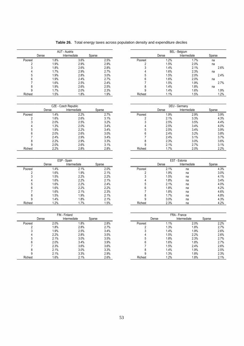
53

Table 26. Total energy taxes across population density and expenditure deciles

AUT - Austria BEL - Belgium Dense Intermediate Sparse Dense Intermediate Sparse

Poorest 1.8% 3.6% 2.5% Poorest 1.2% 1.7% na 2 1.9% 2.9% 2.9% 2 1.5% 2.0% na 3 1.8% 2.6% 2.8% 3 1.4% 2.1% 2.6% 4 1.7% 2.9% 2.7% 4 1.6% 2.3% na 5 1.9% 2.8% 3.0% 5 1.5% 2.0% 2.4% 6 1.9% 2.4% 2.7% 6 1.6% 2.0% na 7 1.6% 2.5% 2.4% 7 1.5% 1.9% 2.7% 8 1.9% 2.6% 2.5% 8 1.4% 1.8% na 9 1.7% 2.0% 2.3% 9 1.4% 1.6% 1.9%

Richest 1.5% 1.8% 1.9% Richest 1.1% 1.5% 1.2%

CZE - Czech Republic DEU - Germany Dense Intermediate Sparse Dense Intermediate Sparse

Poorest 1.4% 2.2% 2.7% Poorest 1.9% 2.9% 3.9% 2 1.6% 2.6% 3.1% 2 2.1% 3.3% 4.3% 3 2.0% 2.5% 3.2% 3 2.5% 3.5% 4.4% 4 1.3% 2.0% 3.4% 4 2.5% 3.4% 4.0% 5 1.9% 2.2% 3.4% 5 2.5% 3.4% 3.9% 6 2.0% 2.6% 3.0% 6 2.4% 3.2% 3.8% 7 2.4% 2.9% 3.4% 7 2.4% 3.1% 3.7% 8 2.2% 2.9% 3.3% 8 2.3% 3.0% 3.6% 9 2.0% 2.6% 3.1% 9 2.1% 2.7% 3.1%

Richest 2.2% 2.8% 2.8% Richest 1.7% 2.0% 2.2%

ESP - Spain EST - Estonia Dense Intermediate Sparse Dense Intermediate Sparse

Poorest 1.4% 2.1% 2.0% Poorest 2.1% na 4.3% 2 1.6% 1.9% 2.1% 2 1.9% na 3.0% 3 1.5% 2.2% 2.2% 3 1.5% na 4.1% 4 1.6% 2.2% 2.1% 4 1.8% na 3.4% 5 1.6% 2.2% 2.4% 5 2.1% na 4.0% 6 1.6% 2.2% 2.2% 6 1.8% na 4.2% 7 1.6% 2.1% 2.3% 7 1.8% na 4.6% 8 1.5% 1.9% 2.1% 8 1.7% na 4.8% 9 1.4% 1.8% 2.1% 9 3.0% na 4.3%

Richest 1.2% 1.7% 1.5% Richest 2.3% na 4.2%

FIN - Finland FRA - France Dense Intermediate Sparse Dense Intermediate Sparse

Poorest 2.0% 1.8% 2.8% Poorest 1.1% 2.0% 2.2% 2 1.8% 2.8% 2.7% 2 1.3% 1.8% 2.7% 3 1.9% 2.5% 3.4% 3 1.4% 1.9% 2.6% 4 2.2% 2.8% 3.5% 4 1.5% 2.2% 2.6% 5 2.1% 3.0% 3.5% 5 1.8% 2.3% 2.7% 6 2.0% 3.4% 3.9% 6 1.6% 1.8% 2.7% 7 2.3% 3.6% 3.6% 7 1.5% 2.4% 2.6% 8 2.1% 3.0% 3.3% 8 1.4% 1.9% 2.5% 9 2.1% 3.3% 2.9% 9 1.3% 1.8% 2.3%

Richest 1.6% 2.1% 2.6% Richest 1.2% 1.8% 2.1%

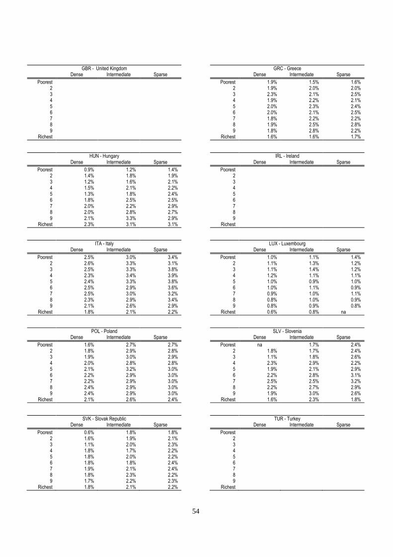
54

GBR - United Kingdom GRC - Greece Dense Intermediate Sparse Dense Intermediate Sparse

Poorest Poorest 1.9% 1.5% 1.6% 2 2 1.9% 2.0% 2.0% 3 3 2.3% 2.1% 2.5% 4 4 1.9% 2.2% 2.1% 5 5 2.0% 2.3% 2.4% 6 6 2.0% 2.1% 2.5% 7 7 1.8% 2.2% 2.2% 8 8 1.9% 2.5% 2.8% 9 9 1.8% 2.8% 2.2%

Richest Richest 1.6% 1.6% 1.7%

HUN - Hungary IRL - Ireland Dense Intermediate Sparse Dense Intermediate Sparse

Poorest 0.9% 1.2% 1.4% Poorest 2 1.4% 1.8% 1.9% 2 3 1.2% 1.6% 2.1% 3 4 1.5% 2.1% 2.2% 4 5 1.3% 1.8% 2.4% 5 6 1.8% 2.5% 2.5% 6 7 2.0% 2.2% 2.9% 7 8 2.0% 2.8% 2.7% 8 9 2.1% 3.3% 2.9% 9

Richest 2.3% 3.1% 3.1% Richest

ITA - Italy LUX - Luxembourg Dense Intermediate Sparse Dense Intermediate Sparse

Poorest 2.5% 3.0% 3.4% Poorest 1.0% 1.1% 1.4% 2 2.6% 3.3% 3.1% 2 1.1% 1.3% 1.2% 3 2.5% 3.3% 3.8% 3 1.1% 1.4% 1.2% 4 2.3% 3.4% 3.9% 4 1.2% 1.1% 1.1% 5 2.4% 3.3% 3.8% 5 1.0% 0.9% 1.0% 6 2.5% 2.9% 3.6% 6 1.0% 1.1% 0.9% 7 2.5% 3.0% 3.2% 7 0.9% 1.0% 1.1% 8 2.3% 2.9% 3.4% 8 0.8% 1.0% 0.9% 9 2.1% 2.6% 2.9% 9 0.8% 0.9% 0.8%

Richest 1.8% 2.1% 2.2% Richest 0.6% 0.8% na

POL - Poland SLV - Slovenia Dense Intermediate Sparse Dense Intermediate Sparse

Poorest 1.6% 2.7% 2.7% Poorest na 1.7% 2.4% 2 1.8% 2.9% 2.8% 2 1.8% 1.7% 2.4% 3 1.9% 3.0% 2.9% 3 1.1% 1.8% 2.6% 4 2.0% 2.8% 2.8% 4 2.3% 2.9% 2.2% 5 2.1% 3.2% 3.0% 5 1.9% 2.1% 2.9% 6 2.2% 2.9% 3.0% 6 2.2% 2.8% 3.1% 7 2.2% 2.9% 3.0% 7 2.5% 2.5% 3.2% 8 2.4% 2.9% 3.0% 8 2.2% 2.7% 2.9% 9 2.4% 2.9% 3.0% 9 1.9% 3.0% 2.6%

Richest 2.1% 2.6% 2.4% Richest 1.6% 2.3% 1.8%

SVK - Slovak Republic TUR - Turkey Dense Intermediate Sparse Dense Intermediate Sparse

Poorest 0.6% 1.8% 1.8% Poorest 2 1.6% 1.9% 2.1% 2 3 1.1% 2.0% 2.3% 3 4 1.8% 1.7% 2.2% 4 5 1.8% 2.0% 2.2% 5 6 1.8% 1.8% 2.4% 6 7 1.9% 2.1% 2.4% 7 8 1.8% 2.3% 2.2% 8 9 1.7% 2.2% 2.3% 9

Richest 1.8% 2.1% 2.2% Richest

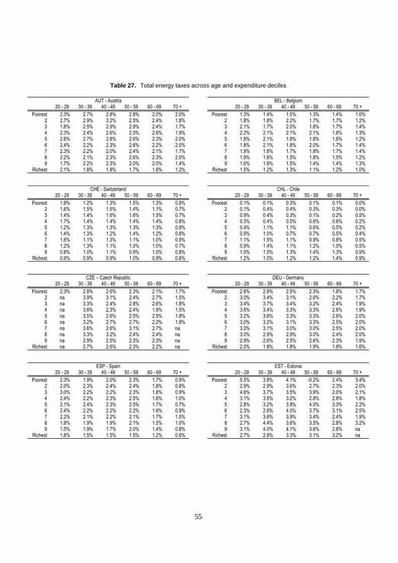
55

Table 27. Total energy taxes across age and expenditure deciles

AUT - Austria BEL - Belgium 20 - 29 30 - 39 40 - 49 50 - 59 60 - 69 70 + 20 - 29 30 - 39 40 - 49 50 - 59 60 - 69 70 +

Poorest 2.3% 2.7% 2.8% 2.8% 2.0% 2.0% Poorest 1.3% 1.4% 1.5% 1.3% 1.4% 1.0% 2 2.7% 2.9% 3.2% 2.5% 2.4% 1.8% 2 1.8% 1.8% 2.2% 1.7% 1.7% 1.2% 3 1.8% 2.5% 2.9% 2.9% 2.4% 1.7% 3 2.1% 1.7% 2.0% 1.8% 1.7% 1.4% 4 2.3% 2.4% 2.6% 2.5% 2.6% 1.9% 4 2.2% 2.1% 2.1% 2.1% 1.8% 1.3% 5 2.6% 2.7% 2.8% 2.6% 2.3% 2.0% 5 1.8% 2.1% 1.8% 1.8% 1.6% 1.2% 6 2.4% 2.2% 2.3% 2.6% 2.2% 2.0% 6 1.8% 2.1% 1.8% 2.0% 1.7% 1.4% 7 2.3% 2.2% 2.0% 2.4% 2.1% 1.7% 7 1.9% 1.8% 1.7% 1.8% 1.7% 1.4% 8 2.2% 2.1% 2.3% 2.6% 2.3% 2.0% 8 1.9% 1.6% 1.5% 1.8% 1.5% 1.2% 9 1.7% 2.2% 2.3% 2.0% 2.0% 1.4% 9 1.6% 1.6% 1.5% 1.4% 1.4% 1.3%

Richest 2.1% 1.8% 1.8% 1.7% 1.6% 1.2% Richest 1.5% 1.2% 1.3% 1.1% 1.2% 1.0%

CHE - Switzerland CHL - Chile 20 - 29 30 - 39 40 - 49 50 - 59 60 - 69 70 + 20 - 29 30 - 39 40 - 49 50 - 59 60 - 69 70 +

Poorest 1.8% 1.2% 1.3% 1.5% 1.3% 0.8% Poorest 0.1% 0.1% 0.3% 0.1% 0.1% 0.0% 2 1.6% 1.5% 1.5% 1.4% 1.1% 0.7% 2 0.1% 0.4% 0.4% 0.3% 0.3% 0.0% 3 1.4% 1.4% 1.6% 1.6% 1.5% 0.7% 3 0.9% 0.4% 0.3% 0.1% 0.2% 0.5% 4 1.7% 1.4% 1.4% 1.4% 1.4% 0.8% 4 0.3% 0.4% 0.5% 0.6% 0.6% 0.2% 5 1.2% 1.3% 1.3% 1.3% 1.3% 0.8% 5 0.4% 1.1% 1.1% 0.6% 0.5% 0.2% 6 1.4% 1.3% 1.2% 1.4% 1.2% 0.8% 6 0.9% 1.0% 0.7% 0.7% 0.5% 0.4% 7 1.6% 1.1% 1.3% 1.1% 1.0% 0.9% 7 1.1% 1.5% 1.1% 0.9% 0.8% 0.5% 8 1.2% 1.3% 1.1% 1.0% 1.0% 0.7% 8 0.9% 1.4% 1.1% 1.2% 1.0% 0.5% 9 0.8% 1.0% 1.1% 0.9% 1.0% 0.8% 9 1.0% 1.5% 1.3% 1.4% 1.3% 0.9%

Richest 0.9% 0.9% 0.9% 1.0% 0.9% 0.6% Richest 1.2% 1.0% 1.2% 1.2% 1.4% 0.9%

CZE – Czech Republic DEU - Germany 20 - 29 30 - 39 40 - 49 50 - 59 60 - 69 70 + 20 - 29 30 - 39 40 - 49 50 - 59 60 - 69 70 +

Poorest 2.3% 2.8% 2.6% 2.3% 2.1% 1.7% Poorest 2.8% 2.8% 2.5% 2.3% 1.8% 1.7% 2 na 3.9% 3.1% 2.4% 2.7% 1.5% 2 3.0% 3.4% 3.1% 2.6% 2.2% 1.7% 3 na 3.3% 2.4% 2.8% 2.6% 1.8% 3 3.4% 3.7% 3.4% 3.2% 2.4% 1.9% 4 na 3.6% 2.3% 2.4% 1.9% 1.5% 4 3.6% 3.4% 3.3% 3.3% 2.6% 1.9% 5 na 3.5% 2.6% 2.5% 2.5% 1.8% 5 3.2% 3.6% 3.3% 3.3% 2.6% 2.0% 6 na 3.2% 2.7% 2.7% 2.2% 1.8% 6 3.0% 3.2% 3.1% 3.3% 2.5% 2.0% 7 na 3.6% 2.6% 3.1% 2.7% na 7 3.3% 3.1% 3.0% 3.0% 2.5% 2.0% 8 na 3.3% 3.2% 2.4% 2.4% na 8 3.0% 2.9% 2.9% 3.0% 2.4% 2.0% 9 na 2.9% 2.5% 2.3% 2.3% na 9 2.9% 2.6% 2.5% 2.6% 2.3% 1.9%

Richest na 2.7% 2.6% 2.3% 2.2% na Richest 2.0% 1.8% 1.8% 1.9% 1.8% 1.6%

ESP - Spain EST - Estonia 20 - 29 30 - 39 40 - 49 50 - 59 60 - 69 70 + 20 - 29 30 - 39 40 - 49 50 - 59 60 - 69 70 +

Poorest 2.3% 1.9% 2.0% 2.3% 1.7% 0.9% Poorest 5.5% 3.8% 4.1% -0.2% 2.4% 3.4% 2 2.0% 2.3% 2.4% 2.4% 1.8% 0.8% 2 2.9% 2.9% 3.6% 2.7% 2.3% 2.0% 3 3.0% 2.2% 2.2% 2.3% 1.8% 0.9% 3 4.6% 3.7% 3.5% 3.9% 2.0% 2.1% 4 2.4% 2.2% 2.3% 2.5% 1.6% 1.0% 4 3.1% 3.5% 3.2% 2.8% 2.8% 1.8% 5 2.1% 2.4% 2.3% 2.5% 1.7% 0.7% 5 2.8% 3.2% 3.8% 4.0% 3.3% 2.2% 6 2.4% 2.2% 2.2% 2.2% 1.6% 0.9% 6 2.3% 2.6% 4.0% 3.7% 3.1% 2.5% 7 2.2% 2.1% 2.2% 2.1% 1.7% 1.0% 7 3.1% 3.6% 3.9% 3.4% 2.4% 1.9% 8 1.8% 1.9% 1.9% 2.1% 1.5% 1.0% 8 2.7% 4.4% 3.6% 3.5% 2.8% 3.2% 9 1.5% 1.9% 1.7% 2.0% 1.4% 0.8% 9 3.1% 4.0% 4.1% 3.6% 2.8% na

Richest 1.8% 1.5% 1.5% 1.5% 1.2% 0.6% Richest 2.7% 2.8% 3.3% 3.1% 3.2% na

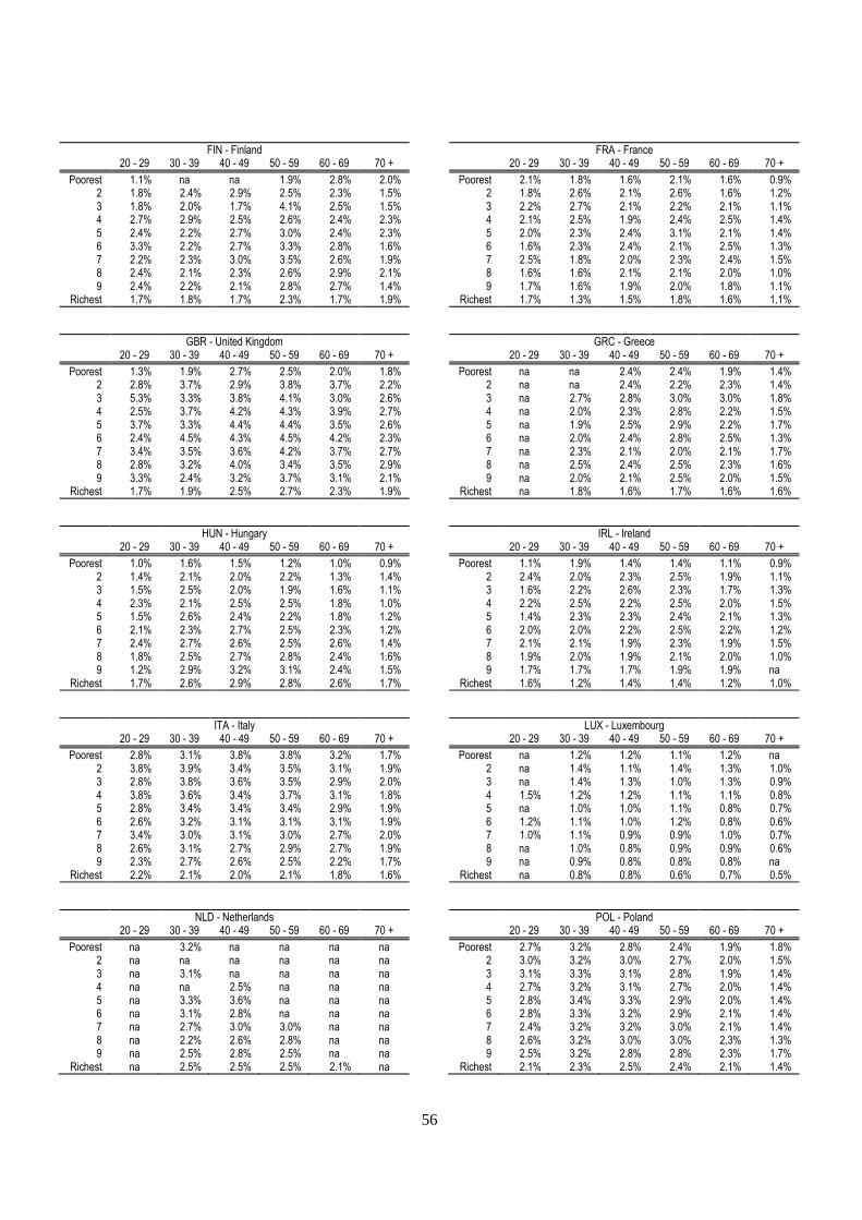
56

FIN - Finland FRA - France 20 - 29 30 - 39 40 - 49 50 - 59 60 - 69 70 + 20 - 29 30 - 39 40 - 49 50 - 59 60 - 69 70 +

Poorest 1.1% na na 1.9% 2.8% 2.0% Poorest 2.1% 1.8% 1.6% 2.1% 1.6% 0.9% 2 1.8% 2.4% 2.9% 2.5% 2.3% 1.5% 2 1.8% 2.6% 2.1% 2.6% 1.6% 1.2% 3 1.8% 2.0% 1.7% 4.1% 2.5% 1.5% 3 2.2% 2.7% 2.1% 2.2% 2.1% 1.1% 4 2.7% 2.9% 2.5% 2.6% 2.4% 2.3% 4 2.1% 2.5% 1.9% 2.4% 2.5% 1.4% 5 2.4% 2.2% 2.7% 3.0% 2.4% 2.3% 5 2.0% 2.3% 2.4% 3.1% 2.1% 1.4% 6 3.3% 2.2% 2.7% 3.3% 2.8% 1.6% 6 1.6% 2.3% 2.4% 2.1% 2.5% 1.3% 7 2.2% 2.3% 3.0% 3.5% 2.6% 1.9% 7 2.5% 1.8% 2.0% 2.3% 2.4% 1.5% 8 2.4% 2.1% 2.3% 2.6% 2.9% 2.1% 8 1.6% 1.6% 2.1% 2.1% 2.0% 1.0% 9 2.4% 2.2% 2.1% 2.8% 2.7% 1.4% 9 1.7% 1.6% 1.9% 2.0% 1.8% 1.1%

Richest 1.7% 1.8% 1.7% 2.3% 1.7% 1.9% Richest 1.7% 1.3% 1.5% 1.8% 1.6% 1.1%

GBR - United Kingdom GRC - Greece 20 - 29 30 - 39 40 - 49 50 - 59 60 - 69 70 + 20 - 29 30 - 39 40 - 49 50 - 59 60 - 69 70 +

Poorest 1.3% 1.9% 2.7% 2.5% 2.0% 1.8% Poorest na na 2.4% 2.4% 1.9% 1.4% 2 2.8% 3.7% 2.9% 3.8% 3.7% 2.2% 2 na na 2.4% 2.2% 2.3% 1.4% 3 5.3% 3.3% 3.8% 4.1% 3.0% 2.6% 3 na 2.7% 2.8% 3.0% 3.0% 1.8% 4 2.5% 3.7% 4.2% 4.3% 3.9% 2.7% 4 na 2.0% 2.3% 2.8% 2.2% 1.5% 5 3.7% 3.3% 4.4% 4.4% 3.5% 2.6% 5 na 1.9% 2.5% 2.9% 2.2% 1.7% 6 2.4% 4.5% 4.3% 4.5% 4.2% 2.3% 6 na 2.0% 2.4% 2.8% 2.5% 1.3% 7 3.4% 3.5% 3.6% 4.2% 3.7% 2.7% 7 na 2.3% 2.1% 2.0% 2.1% 1.7% 8 2.8% 3.2% 4.0% 3.4% 3.5% 2.9% 8 na 2.5% 2.4% 2.5% 2.3% 1.6% 9 3.3% 2.4% 3.2% 3.7% 3.1% 2.1% 9 na 2.0% 2.1% 2.5% 2.0% 1.5%

Richest 1.7% 1.9% 2.5% 2.7% 2.3% 1.9% Richest na 1.8% 1.6% 1.7% 1.6% 1.6%

HUN - Hungary IRL - Ireland 20 - 29 30 - 39 40 - 49 50 - 59 60 - 69 70 + 20 - 29 30 - 39 40 - 49 50 - 59 60 - 69 70 +

Poorest 1.0% 1.6% 1.5% 1.2% 1.0% 0.9% Poorest 1.1% 1.9% 1.4% 1.4% 1.1% 0.9% 2 1.4% 2.1% 2.0% 2.2% 1.3% 1.4% 2 2.4% 2.0% 2.3% 2.5% 1.9% 1.1% 3 1.5% 2.5% 2.0% 1.9% 1.6% 1.1% 3 1.6% 2.2% 2.6% 2.3% 1.7% 1.3% 4 2.3% 2.1% 2.5% 2.5% 1.8% 1.0% 4 2.2% 2.5% 2.2% 2.5% 2.0% 1.5% 5 1.5% 2.6% 2.4% 2.2% 1.8% 1.2% 5 1.4% 2.3% 2.3% 2.4% 2.1% 1.3% 6 2.1% 2.3% 2.7% 2.5% 2.3% 1.2% 6 2.0% 2.0% 2.2% 2.5% 2.2% 1.2% 7 2.4% 2.7% 2.6% 2.5% 2.6% 1.4% 7 2.1% 2.1% 1.9% 2.3% 1.9% 1.5% 8 1.8% 2.5% 2.7% 2.8% 2.4% 1.6% 8 1.9% 2.0% 1.9% 2.1% 2.0% 1.0% 9 1.2% 2.9% 3.2% 3.1% 2.4% 1.5% 9 1.7% 1.7% 1.7% 1.9% 1.9% na

Richest 1.7% 2.6% 2.9% 2.8% 2.6% 1.7% Richest 1.6% 1.2% 1.4% 1.4% 1.2% 1.0%

ITA - Italy LUX - Luxembourg 20 - 29 30 - 39 40 - 49 50 - 59 60 - 69 70 + 20 - 29 30 - 39 40 - 49 50 - 59 60 - 69 70 +

Poorest 2.8% 3.1% 3.8% 3.8% 3.2% 1.7% Poorest na 1.2% 1.2% 1.1% 1.2% na 2 3.8% 3.9% 3.4% 3.5% 3.1% 1.9% 2 na 1.4% 1.1% 1.4% 1.3% 1.0% 3 2.8% 3.8% 3.6% 3.5% 2.9% 2.0% 3 na 1.4% 1.3% 1.0% 1.3% 0.9% 4 3.8% 3.6% 3.4% 3.7% 3.1% 1.8% 4 1.5% 1.2% 1.2% 1.1% 1.1% 0.8% 5 2.8% 3.4% 3.4% 3.4% 2.9% 1.9% 5 na 1.0% 1.0% 1.1% 0.8% 0.7% 6 2.6% 3.2% 3.1% 3.1% 3.1% 1.9% 6 1.2% 1.1% 1.0% 1.2% 0.8% 0.6% 7 3.4% 3.0% 3.1% 3.0% 2.7% 2.0% 7 1.0% 1.1% 0.9% 0.9% 1.0% 0.7% 8 2.6% 3.1% 2.7% 2.9% 2.7% 1.9% 8 na 1.0% 0.8% 0.9% 0.9% 0.6% 9 2.3% 2.7% 2.6% 2.5% 2.2% 1.7% 9 na 0.9% 0.8% 0.8% 0.8% na

Richest 2.2% 2.1% 2.0% 2.1% 1.8% 1.6% Richest na 0.8% 0.8% 0.6% 0.7% 0.5%

NLD - Netherlands POL - Poland 20 - 29 30 - 39 40 - 49 50 - 59 60 - 69 70 + 20 - 29 30 - 39 40 - 49 50 - 59 60 - 69 70 +

Poorest na 3.2% na na na na Poorest 2.7% 3.2% 2.8% 2.4% 1.9% 1.8% 2 na na na na na na 2 3.0% 3.2% 3.0% 2.7% 2.0% 1.5% 3 na 3.1% na na na na 3 3.1% 3.3% 3.1% 2.8% 1.9% 1.4% 4 na na 2.5% na na na 4 2.7% 3.2% 3.1% 2.7% 2.0% 1.4% 5 na 3.3% 3.6% na na na 5 2.8% 3.4% 3.3% 2.9% 2.0% 1.4% 6 na 3.1% 2.8% na na na 6 2.8% 3.3% 3.2% 2.9% 2.1% 1.4% 7 na 2.7% 3.0% 3.0% na na 7 2.4% 3.2% 3.2% 3.0% 2.1% 1.4% 8 na 2.2% 2.6% 2.8% na na 8 2.6% 3.2% 3.0% 3.0% 2.3% 1.3% 9 na 2.5% 2.8% 2.5% na na 9 2.5% 3.2% 2.8% 2.8% 2.3% 1.7%

Richest na 2.5% 2.5% 2.5% 2.1% na Richest 2.1% 2.3% 2.5% 2.4% 2.1% 1.4%

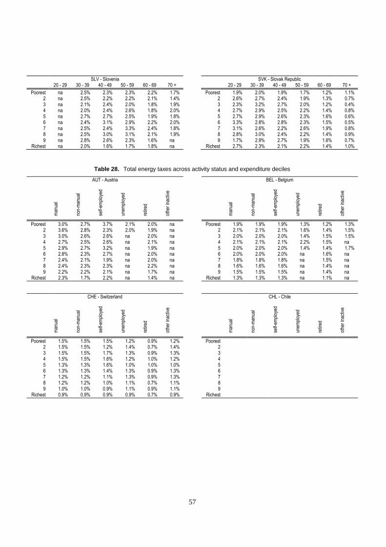
57

SLV - Slovenia SVK - Slovak Republic 20 - 29 30 - 39 40 - 49 50 - 59 60 - 69 70 + 20 - 29 30 - 39 40 - 49 50 - 59 60 - 69 70 +

Poorest na 2.5% 2.3% 2.3% 2.2% 1.7% Poorest 1.9% 2.0% 1.9% 1.7% 1.2% 1.1% 2 na 2.5% 2.2% 2.2% 2.1% 1.4% 2 2.6% 2.7% 2.4% 1.9% 1.3% 0.7% 3 na 2.1% 2.4% 2.0% 1.8% 1.9% 3 2.3% 3.2% 2.7% 2.0% 1.2% 0.4% 4 na 2.0% 2.4% 2.6% 1.8% 2.0% 4 2.7% 2.9% 2.5% 2.2% 1.4% 0.8% 5 na 2.7% 2.7% 2.5% 1.9% 1.8% 5 2.7% 2.9% 2.6% 2.3% 1.6% 0.6% 6 na 2.4% 3.1% 2.9% 2.2% 2.0% 6 3.3% 2.8% 2.8% 2.3% 1.5% 0.5% 7 na 2.5% 2.4% 3.3% 2.4% 1.8% 7 3.1% 2.6% 2.2% 2.6% 1.9% 0.8% 8 na 2.5% 3.0% 3.1% 2.1% 1.9% 8 2.8% 3.0% 2.4% 2.2% 1.4% 0.9% 9 na 2.8% 2.6% 2.3% 1.6% na 9 1.7% 2.9% 2.7% 1.9% 1.6% 0.7%

Richest na 2.0% 1.6% 1.7% 1.8% na Richest 2.7% 2.3% 2.1% 2.2% 1.4% 1.0%

Table 28. Total energy taxes across activity status and expenditure deciles

AUT - Austria BEL - Belgium

man

ual

non-

man

ual

self-

empl

oyed

unem

ploy

ed

retir

ed

othe

r in

activ

e

man

ual

non-

man

ual

self-

empl

oyed

unem

ploy

ed

retir

ed

othe

r in

activ

e

Poorest 3.0% 2.7% 3.7% 2.1% 2.0% na Poorest 1.9% 1.9% 1.9% 1.3% 1.2% 1.3% 2 3.6% 2.8% 2.3% 2.0% 1.9% na 2 2.1% 2.1% 2.1% 1.6% 1.4% 1.5% 3 3.0% 2.6% 2.6% na 2.0% na 3 2.0% 2.0% 2.0% 1.4% 1.5% 1.5% 4 2.7% 2.5% 2.6% na 2.1% na 4 2.1% 2.1% 2.1% 2.2% 1.5% na 5 2.9% 2.7% 3.2% na 1.9% na 5 2.0% 2.0% 2.0% 1.4% 1.4% 1.7% 6 2.8% 2.3% 2.7% na 2.0% na 6 2.0% 2.0% 2.0% na 1.6% na 7 2.4% 2.1% 1.9% na 2.0% na 7 1.8% 1.8% 1.8% na 1.5% na 8 2.4% 2.3% 2.3% na 2.2% na 8 1.6% 1.6% 1.6% na 1.4% na 9 2.2% 2.2% 2.1% na 1.7% na 9 1.5% 1.5% 1.5% na 1.4% na

Richest 2.3% 1.7% 2.2% na 1.4% na Richest 1.3% 1.3% 1.3% na 1.1% na

CHE - Switzerland CHL - Chile

man

ual

non-

man

ual

self-

empl

oyed

unem

ploy

ed

retir

ed

othe

r in

activ

e

man

ual

non-

man

ual

self-

empl

oyed

unem

ploy

ed

retir

ed

othe

r in

activ

e Poorest 1.5% 1.5% 1.5% 1.2% 0.9% 1.2% Poorest

2 1.5% 1.5% 1.2% 1.4% 0.7% 1.4% 2 3 1.5% 1.5% 1.7% 1.3% 0.9% 1.3% 3 4 1.5% 1.5% 1.6% 1.2% 1.0% 1.2% 4 5 1.3% 1.3% 1.6% 1.0% 1.0% 1.0% 5 6 1.3% 1.3% 1.4% 1.3% 0.9% 1.3% 6 7 1.2% 1.2% 1.1% 1.3% 0.9% 1.3% 7 8 1.2% 1.2% 1.0% 1.1% 0.7% 1.1% 8 9 1.0% 1.0% 0.9% 1.1% 0.9% 1.1% 9

Richest 0.9% 0.9% 0.9% 0.9% 0.7% 0.9% Richest

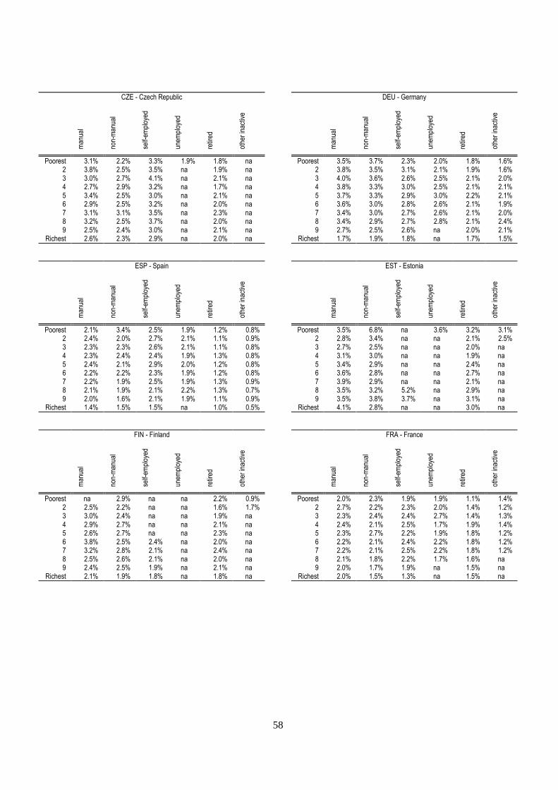
58

CZE - Czech Republic DEU - Germany

man

ual

non-

man

ual

self-

empl

oyed

unem

ploy

ed

retir

ed

othe

r in

activ

e

man

ual

non-

man

ual

self-

empl

oyed

unem

ploy

ed

retir

ed

othe

r in

activ

e

Poorest 3.1% 2.2% 3.3% 1.9% 1.8% na Poorest 3.5% 3.7% 2.3% 2.0% 1.8% 1.6% 2 3.8% 2.5% 3.5% na 1.9% na 2 3.8% 3.5% 3.1% 2.1% 1.9% 1.6% 3 3.0% 2.7% 4.1% na 2.1% na 3 4.0% 3.6% 2.6% 2.5% 2.1% 2.0% 4 2.7% 2.9% 3.2% na 1.7% na 4 3.8% 3.3% 3.0% 2.5% 2.1% 2.1% 5 3.4% 2.5% 3.0% na 2.1% na 5 3.7% 3.3% 2.9% 3.0% 2.2% 2.1% 6 2.9% 2.5% 3.2% na 2.0% na 6 3.6% 3.0% 2.8% 2.6% 2.1% 1.9% 7 3.1% 3.1% 3.5% na 2.3% na 7 3.4% 3.0% 2.7% 2.6% 2.1% 2.0% 8 3.2% 2.5% 3.7% na 2.0% na 8 3.4% 2.9% 2.7% 2.8% 2.1% 2.4% 9 2.5% 2.4% 3.0% na 2.1% na 9 2.7% 2.5% 2.6% na 2.0% 2.1%

Richest 2.6% 2.3% 2.9% na 2.0% na Richest 1.7% 1.9% 1.8% na 1.7% 1.5%

ESP - Spain EST - Estonia

man

ual

non-

man

ual

self-

empl

oyed

unem

ploy

ed

retir

ed

othe

r in

activ

e

man

ual

non-

man

ual

self-

empl

oyed

unem

ploy

ed

retir

ed

othe

r in

activ

e

Poorest 2.1% 3.4% 2.5% 1.9% 1.2% 0.8% Poorest 3.5% 6.8% na 3.6% 3.2% 3.1% 2 2.4% 2.0% 2.7% 2.1% 1.1% 0.9% 2 2.8% 3.4% na na 2.1% 2.5% 3 2.3% 2.3% 2.6% 2.1% 1.1% 0.8% 3 2.7% 2.5% na na 2.0% na 4 2.3% 2.4% 2.4% 1.9% 1.3% 0.8% 4 3.1% 3.0% na na 1.9% na 5 2.4% 2.1% 2.9% 2.0% 1.2% 0.8% 5 3.4% 2.9% na na 2.4% na 6 2.2% 2.2% 2.3% 1.9% 1.2% 0.8% 6 3.6% 2.8% na na 2.7% na 7 2.2% 1.9% 2.5% 1.9% 1.3% 0.9% 7 3.9% 2.9% na na 2.1% na 8 2.1% 1.9% 2.1% 2.2% 1.3% 0.7% 8 3.5% 3.2% 5.2% na 2.9% na 9 2.0% 1.6% 2.1% 1.9% 1.1% 0.9% 9 3.5% 3.8% 3.7% na 3.1% na

Richest 1.4% 1.5% 1.5% na 1.0% 0.5% Richest 4.1% 2.8% na na 3.0% na

FIN - Finland FRA - France

man

ual

non-

man

ual

self-

empl

oyed

unem

ploy

ed

retir

ed

othe

r in

activ

e

man

ual

non-

man

ual

self-

empl

oyed

unem

ploy

ed

retir

ed

othe

r in

activ

e Poorest na 2.9% na na 2.2% 0.9% Poorest 2.0% 2.3% 1.9% 1.9% 1.1% 1.4%

2 2.5% 2.2% na na 1.6% 1.7% 2 2.7% 2.2% 2.3% 2.0% 1.4% 1.2% 3 3.0% 2.4% na na 1.9% na 3 2.3% 2.4% 2.4% 2.7% 1.4% 1.3% 4 2.9% 2.7% na na 2.1% na 4 2.4% 2.1% 2.5% 1.7% 1.9% 1.4% 5 2.6% 2.7% na na 2.3% na 5 2.3% 2.7% 2.2% 1.9% 1.8% 1.2% 6 3.8% 2.5% 2.4% na 2.0% na 6 2.2% 2.1% 2.4% 2.2% 1.8% 1.2% 7 3.2% 2.8% 2.1% na 2.4% na 7 2.2% 2.1% 2.5% 2.2% 1.8% 1.2% 8 2.5% 2.6% 2.1% na 2.0% na 8 2.1% 1.8% 2.2% 1.7% 1.6% na 9 2.4% 2.5% 1.9% na 2.1% na 9 2.0% 1.7% 1.9% na 1.5% na

Richest 2.1% 1.9% 1.8% na 1.8% na Richest 2.0% 1.5% 1.3% na 1.5% na

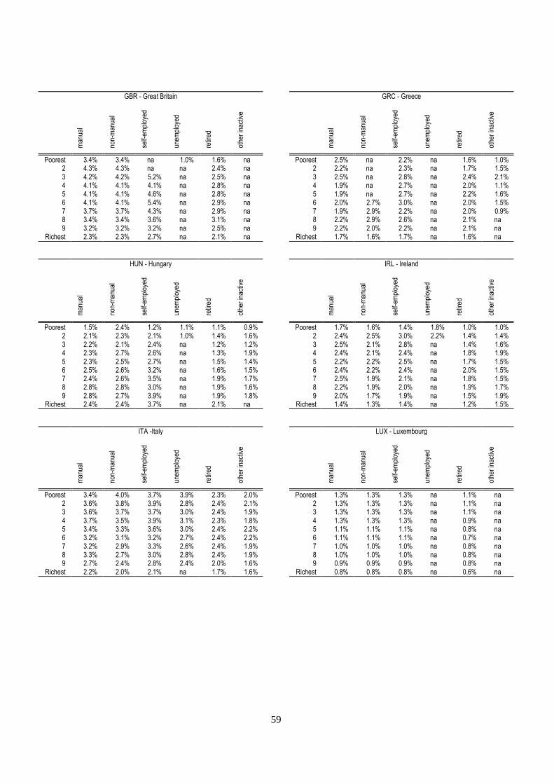
59

GBR - Great Britain GRC - Greece

man

ual

non-

man

ual

self-

empl

oyed

unem

ploy

ed

retir

ed

othe

r in

activ

e

man

ual

non-

man

ual

self-

empl

oyed

unem

ploy

ed

retir

ed

othe

r in

activ

e

Poorest 3.4% 3.4% na 1.0% 1.6% na Poorest 2.5% na 2.2% na 1.6% 1.0% 2 4.3% 4.3% na na 2.4% na 2 2.2% na 2.3% na 1.7% 1.5% 3 4.2% 4.2% 5.2% na 2.5% na 3 2.5% na 2.8% na 2.4% 2.1% 4 4.1% 4.1% 4.1% na 2.8% na 4 1.9% na 2.7% na 2.0% 1.1% 5 4.1% 4.1% 4.6% na 2.8% na 5 1.9% na 2.7% na 2.2% 1.6% 6 4.1% 4.1% 5.4% na 2.9% na 6 2.0% 2.7% 3.0% na 2.0% 1.5% 7 3.7% 3.7% 4.3% na 2.9% na 7 1.9% 2.9% 2.2% na 2.0% 0.9% 8 3.4% 3.4% 3.6% na 3.1% na 8 2.2% 2.9% 2.6% na 2.1% na 9 3.2% 3.2% 3.2% na 2.5% na 9 2.2% 2.0% 2.2% na 2.1% na

Richest 2.3% 2.3% 2.7% na 2.1% na Richest 1.7% 1.6% 1.7% na 1.6% na

HUN - Hungary IRL - Ireland

man

ual

non-

man

ual

self-

empl

oyed

unem

ploy

ed

retir

ed

othe

r in

activ

e

man

ual

non-

man

ual

self-

empl

oyed

unem

ploy

ed

retir

ed

othe

r in

activ

e

Poorest 1.5% 2.4% 1.2% 1.1% 1.1% 0.9% Poorest 1.7% 1.6% 1.4% 1.8% 1.0% 1.0% 2 2.1% 2.3% 2.1% 1.0% 1.4% 1.6% 2 2.4% 2.5% 3.0% 2.2% 1.4% 1.4% 3 2.2% 2.1% 2.4% na 1.2% 1.2% 3 2.5% 2.1% 2.8% na 1.4% 1.6% 4 2.3% 2.7% 2.6% na 1.3% 1.9% 4 2.4% 2.1% 2.4% na 1.8% 1.9% 5 2.3% 2.5% 2.7% na 1.5% 1.4% 5 2.2% 2.2% 2.5% na 1.7% 1.5% 6 2.5% 2.6% 3.2% na 1.6% 1.5% 6 2.4% 2.2% 2.4% na 2.0% 1.5% 7 2.4% 2.6% 3.5% na 1.9% 1.7% 7 2.5% 1.9% 2.1% na 1.8% 1.5% 8 2.8% 2.8% 3.0% na 1.9% 1.6% 8 2.2% 1.9% 2.0% na 1.9% 1.7% 9 2.8% 2.7% 3.9% na 1.9% 1.8% 9 2.0% 1.7% 1.9% na 1.5% 1.9%

Richest 2.4% 2.4% 3.7% na 2.1% na Richest 1.4% 1.3% 1.4% na 1.2% 1.5%

ITA -Italy LUX - Luxembourg

man

ual

non-

man

ual

self-

empl

oyed

unem

ploy

ed

retir

ed

othe

r in

activ

e

man

ual

non-

man

ual

self-

empl

oyed

unem

ploy

ed

retir

ed

othe

r in

activ

e Poorest 3.4% 4.0% 3.7% 3.9% 2.3% 2.0% Poorest 1.3% 1.3% 1.3% na 1.1% na

2 3.6% 3.8% 3.9% 2.8% 2.4% 2.1% 2 1.3% 1.3% 1.3% na 1.1% na 3 3.6% 3.7% 3.7% 3.0% 2.4% 1.9% 3 1.3% 1.3% 1.3% na 1.1% na 4 3.7% 3.5% 3.9% 3.1% 2.3% 1.8% 4 1.3% 1.3% 1.3% na 0.9% na 5 3.4% 3.3% 3.6% 3.0% 2.4% 2.2% 5 1.1% 1.1% 1.1% na 0.8% na 6 3.2% 3.1% 3.2% 2.7% 2.4% 2.2% 6 1.1% 1.1% 1.1% na 0.7% na 7 3.2% 2.9% 3.3% 2.6% 2.4% 1.9% 7 1.0% 1.0% 1.0% na 0.8% na 8 3.3% 2.7% 3.0% 2.8% 2.4% 1.9% 8 1.0% 1.0% 1.0% na 0.8% na 9 2.7% 2.4% 2.8% 2.4% 2.0% 1.6% 9 0.9% 0.9% 0.9% na 0.8% na

Richest 2.2% 2.0% 2.1% na 1.7% 1.6% Richest 0.8% 0.8% 0.8% na 0.6% na

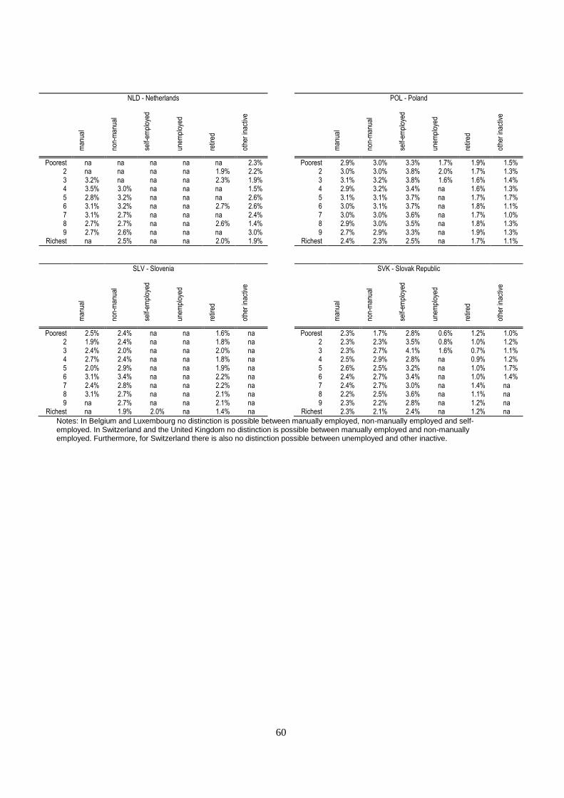
60

NLD - Netherlands POL - Poland

man

ual

non-

man

ual

self-

empl

oyed

unem

ploy

ed

retir

ed

othe

r in

activ

e

man

ual

non-

man

ual

self-

empl

oyed

unem

ploy

ed

retir

ed

othe

r in

activ

e

Poorest na na na na na 2.3% Poorest 2.9% 3.0% 3.3% 1.7% 1.9% 1.5% 2 na na na na 1.9% 2.2% 2 3.0% 3.0% 3.8% 2.0% 1.7% 1.3% 3 3.2% na na na 2.3% 1.9% 3 3.1% 3.2% 3.8% 1.6% 1.6% 1.4% 4 3.5% 3.0% na na na 1.5% 4 2.9% 3.2% 3.4% na 1.6% 1.3% 5 2.8% 3.2% na na na 2.6% 5 3.1% 3.1% 3.7% na 1.7% 1.7% 6 3.1% 3.2% na na 2.7% 2.6% 6 3.0% 3.1% 3.7% na 1.8% 1.1% 7 3.1% 2.7% na na na 2.4% 7 3.0% 3.0% 3.6% na 1.7% 1.0% 8 2.7% 2.7% na na 2.6% 1.4% 8 2.9% 3.0% 3.5% na 1.8% 1.3% 9 2.7% 2.6% na na na 3.0% 9 2.7% 2.9% 3.3% na 1.9% 1.3%

Richest na 2.5% na na 2.0% 1.9% Richest 2.4% 2.3% 2.5% na 1.7% 1.1%

SLV - Slovenia SVK - Slovak Republic

man

ual

non-

man

ual

self-

empl

oyed

unem

ploy

ed

retir

ed

othe

r in

activ

e

man

ual

non-

man

ual

self-

empl

oyed

unem

ploy

ed

retir

ed

othe

r in

activ

e

Poorest 2.5% 2.4% na na 1.6% na Poorest 2.3% 1.7% 2.8% 0.6% 1.2% 1.0% 2 1.9% 2.4% na na 1.8% na 2 2.3% 2.3% 3.5% 0.8% 1.0% 1.2% 3 2.4% 2.0% na na 2.0% na 3 2.3% 2.7% 4.1% 1.6% 0.7% 1.1% 4 2.7% 2.4% na na 1.8% na 4 2.5% 2.9% 2.8% na 0.9% 1.2% 5 2.0% 2.9% na na 1.9% na 5 2.6% 2.5% 3.2% na 1.0% 1.7% 6 3.1% 3.4% na na 2.2% na 6 2.4% 2.7% 3.4% na 1.0% 1.4% 7 2.4% 2.8% na na 2.2% na 7 2.4% 2.7% 3.0% na 1.4% na 8 3.1% 2.7% na na 2.1% na 8 2.2% 2.5% 3.6% na 1.1% na 9 na 2.7% na na 2.1% na 9 2.3% 2.2% 2.8% na 1.2% na

Richest na 1.9% 2.0% na 1.4% na Richest 2.3% 2.1% 2.4% na 1.2% na

Notes: In Belgium and Luxembourg no distinction is possible between manually employed, non-manually employed and self-employed. In Switzerland and the United Kingdom no distinction is possible between manually employed and non-manually employed. Furthermore, for Switzerland there is also no distinction possible between unemployed and other inactive.

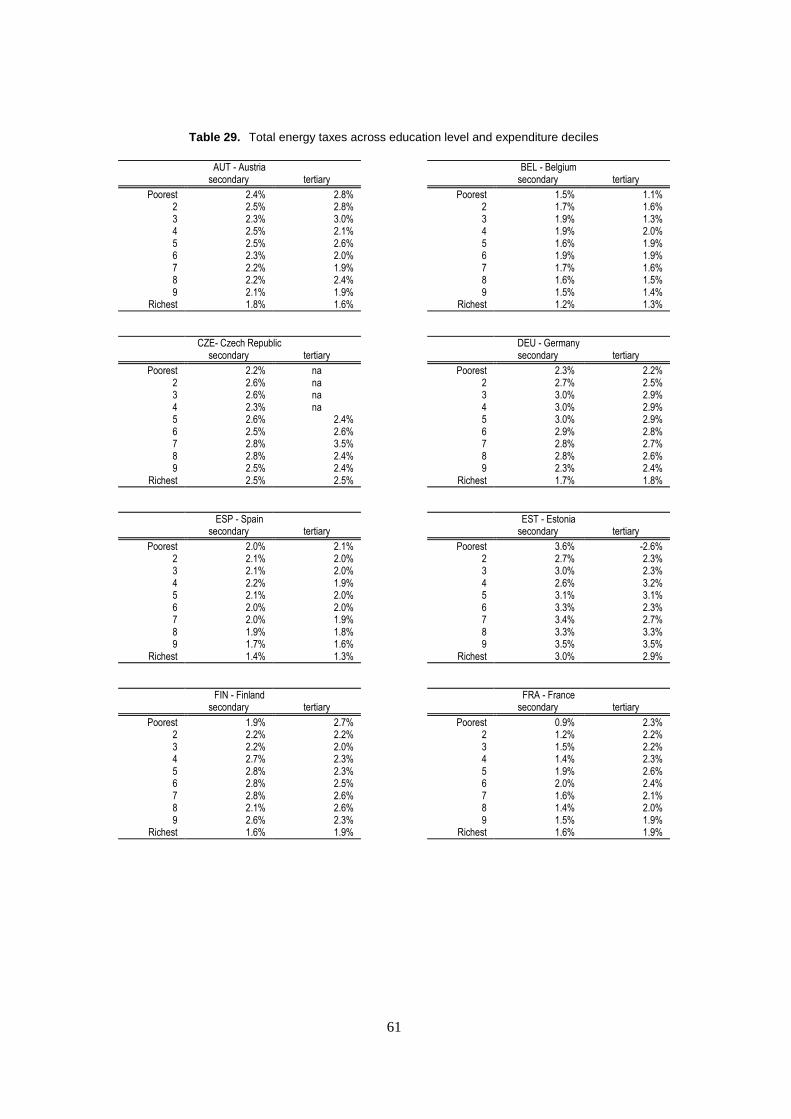
61

Table 29. Total energy taxes across education level and expenditure deciles

AUT - Austria BEL - Belgium secondary tertiary secondary tertiary

Poorest 2.4% 2.8% Poorest 1.5% 1.1% 2 2.5% 2.8% 2 1.7% 1.6% 3 2.3% 3.0% 3 1.9% 1.3% 4 2.5% 2.1% 4 1.9% 2.0% 5 2.5% 2.6% 5 1.6% 1.9% 6 2.3% 2.0% 6 1.9% 1.9% 7 2.2% 1.9% 7 1.7% 1.6% 8 2.2% 2.4% 8 1.6% 1.5% 9 2.1% 1.9% 9 1.5% 1.4%

Richest 1.8% 1.6% Richest 1.2% 1.3%

CZE- Czech Republic DEU - Germany secondary tertiary secondary tertiary

Poorest 2.2% na Poorest 2.3% 2.2% 2 2.6% na 2 2.7% 2.5% 3 2.6% na 3 3.0% 2.9% 4 2.3% na 4 3.0% 2.9% 5 2.6% 2.4% 5 3.0% 2.9% 6 2.5% 2.6% 6 2.9% 2.8% 7 2.8% 3.5% 7 2.8% 2.7% 8 2.8% 2.4% 8 2.8% 2.6% 9 2.5% 2.4% 9 2.3% 2.4%

Richest 2.5% 2.5% Richest 1.7% 1.8%

ESP - Spain EST - Estonia secondary tertiary secondary tertiary

Poorest 2.0% 2.1% Poorest 3.6% -2.6% 2 2.1% 2.0% 2 2.7% 2.3% 3 2.1% 2.0% 3 3.0% 2.3% 4 2.2% 1.9% 4 2.6% 3.2% 5 2.1% 2.0% 5 3.1% 3.1% 6 2.0% 2.0% 6 3.3% 2.3% 7 2.0% 1.9% 7 3.4% 2.7% 8 1.9% 1.8% 8 3.3% 3.3% 9 1.7% 1.6% 9 3.5% 3.5%

Richest 1.4% 1.3% Richest 3.0% 2.9%

FIN - Finland FRA - France secondary tertiary secondary tertiary

Poorest 1.9% 2.7% Poorest 0.9% 2.3% 2 2.2% 2.2% 2 1.2% 2.2% 3 2.2% 2.0% 3 1.5% 2.2% 4 2.7% 2.3% 4 1.4% 2.3% 5 2.8% 2.3% 5 1.9% 2.6% 6 2.8% 2.5% 6 2.0% 2.4% 7 2.8% 2.6% 7 1.6% 2.1% 8 2.1% 2.6% 8 1.4% 2.0% 9 2.6% 2.3% 9 1.5% 1.9%

Richest 1.6% 1.9% Richest 1.6% 1.9%

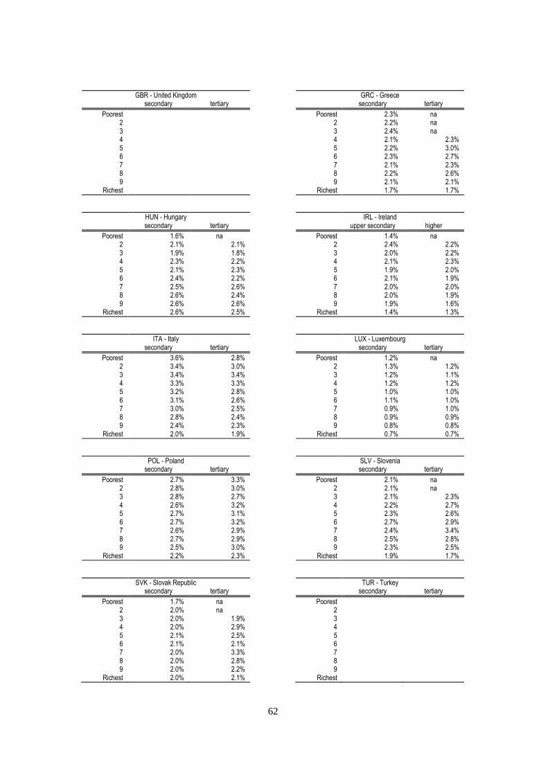
62

GBR - United Kingdom GRC - Greece secondary tertiary secondary tertiary

Poorest Poorest 2.3% na 2 2 2.2% na 3 3 2.4% na 4 4 2.1% 2.3% 5 5 2.2% 3.0% 6 6 2.3% 2.7% 7 7 2.1% 2.3% 8 8 2.2% 2.6% 9 9 2.1% 2.1%

Richest Richest 1.7% 1.7%

HUN - Hungary IRL - Ireland secondary tertiary upper secondary higher

Poorest 1.6% na Poorest 1.4% na 2 2.1% 2.1% 2 2.4% 2.2% 3 1.9% 1.8% 3 2.0% 2.2% 4 2.3% 2.2% 4 2.1% 2.3% 5 2.1% 2.3% 5 1.9% 2.0% 6 2.4% 2.2% 6 2.1% 1.9% 7 2.5% 2.6% 7 2.0% 2.0% 8 2.6% 2.4% 8 2.0% 1.9% 9 2.6% 2.6% 9 1.9% 1.6%

Richest 2.6% 2.5% Richest 1.4% 1.3%

ITA - Italy LUX - Luxembourg secondary tertiary secondary tertiary

Poorest 3.6% 2.8% Poorest 1.2% na 2 3.4% 3.0% 2 1.3% 1.2% 3 3.4% 3.4% 3 1.2% 1.1% 4 3.3% 3.3% 4 1.2% 1.2% 5 3.2% 2.8% 5 1.0% 1.0% 6 3.1% 2.6% 6 1.1% 1.0% 7 3.0% 2.5% 7 0.9% 1.0% 8 2.8% 2.4% 8 0.9% 0.9% 9 2.4% 2.3% 9 0.8% 0.8%

Richest 2.0% 1.9% Richest 0.7% 0.7%

POL - Poland SLV - Slovenia secondary tertiary secondary tertiary

Poorest 2.7% 3.3% Poorest 2.1% na 2 2.8% 3.0% 2 2.1% na 3 2.8% 2.7% 3 2.1% 2.3% 4 2.6% 3.2% 4 2.2% 2.7% 5 2.7% 3.1% 5 2.3% 2.6% 6 2.7% 3.2% 6 2.7% 2.9% 7 2.6% 2.9% 7 2.4% 3.4% 8 2.7% 2.9% 8 2.5% 2.8% 9 2.5% 3.0% 9 2.3% 2.5%

Richest 2.2% 2.3% Richest 1.9% 1.7%

SVK - Slovak Republic TUR - Turkey secondary tertiary secondary tertiary

Poorest 1.7% na Poorest 2 2.0% na 2 3 2.0% 1.9% 3 4 2.0% 2.9% 4 5 2.1% 2.5% 5 6 2.1% 2.1% 6 7 2.0% 3.3% 7 8 2.0% 2.8% 8 9 2.0% 2.2% 9

Richest 2.0% 2.1% Richest

63

ANNEX III

Annex III provides for each country analysed a graph showing the mean shares of taxes on transport

fuels, heating fuels and electricity across expenditure deciles. In addition to Section 3 that provides

information on the mean expenditure on taxes on these energy carriers (Table 3 to Table 9) Figure 23 also

provides confidence intervals.

Confidence intervals allow assessing the degree of uncertainty of an estimate. In this analysis

uncertainty stems mainly from two sources. First, there is uncertainty in about how well the HBS sample

the true population. While providing results across deciles it should be noted that some deciles may be

oversampled while other deciles may be undersampled in the survey. Weights are used to indicate how

much each household contributes to the population average. The confidence intervals reflect that for some

deciles more observations are available to calculate the respective estimate of the population mean, while

for other deciles there are fewer observations. The fewer the observations are the greater is the uncertainty

about the estimate.

Second, there is uncertainty due to different degrees of heterogeneity within each decile. In some

deciles all observed households spend more or less the same amount on energy taxes for the respective

fuels, while in other deciles some households spend a lot while others only a bit or even nothing. The

greater the heterogeneity within deciles is the greater is the uncertainty about the mean estimate for the

respective decile.

Figure 22 shows the 95% confidence intervals for the mean share of taxes on transport fuels, heating

fuels, and electricity in pre-tax expenditure by expenditure decile. A 95% confidence interval should be

interpreted such that there is a 95% chance that the true population mean lies within this interval. The

confidence intervals provide statistical significance for at least two comparisons.

First, for a single energy carrier it can be observed whether the mean expenditure on taxes is

statistically significantly higher or lower than for another decile. For example, Table 4 in Section 3 shows

that the mean estimate for the share of expenditure on transport fuel taxes in Slovenia is 1.7% for the

poorest decile while it is only 1.5% in the richest decile. Figure 23 reveals, however, that this difference is

statistically not significant because the confidence intervals for the poorest and richest decile overlap. In

other words, there is no true difference is measured in the population between the poorest decile and the

richest decile in their expenditure share of transport tax payments. In contrast, for Turkey Table 4 in

Section 3 shows that the poorest decile is estimated to spend 1.1% of expenditure on taxes on transport

fuels while the richest decile is estimated to spend 2.6%. Here the confidence intervals do not overlap as

can be seen in Figure 23. Thus, the poorest decile spends statistically significantly less on taxes on

transport fuels than the richest decile.

Second, the confidence intervals allow assessing whether for a given decile the tax burden differs

between energy carriers. For almost all countries and deciles it is observed that the share of expenditures

on transport fuels in pre-tax expenditure is higher than the shares spend on taxes on heating fuels and on

electricity. The share of expenditures on electricity taxes is higher for some, but not all, countries than the

share of expenditures on taxes on heating fuels, especially for poorer deciles.

Altogether Figure 23 summarises the results presented in Section 4 by country and confirms that the

described results are statistically significant. Taxes on transport fuels are not regressive for most countries.

On the contrary, they are progressive for some countries while they put the highest burden on middle

deciles for others. Taxes on heating fuels are slightly regressive for most, but not all countries. Taxes on

electricity turn out to be regressive for all countries.

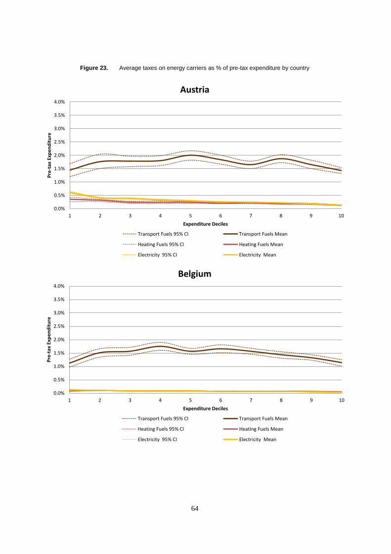
64

Figure 23. Average taxes on energy carriers as % of pre-tax expenditure by country

0.0%

0.5%

1.0%

1.5%

2.0%

2.5%

3.0%

3.5%

4.0%

1 2 3 4 5 6 7 8 9 10

Pre

-tax

Exp

en

dit

ure

Expenditure Deciles

Austria

Transport Fuels 95% CI Transport Fuels Mean

Heating Fuels 95% CI Heating Fuels Mean

Electricity 95% CI Electricity Mean

0.0%

0.5%

1.0%

1.5%

2.0%

2.5%

3.0%

3.5%

4.0%

1 2 3 4 5 6 7 8 9 10

Pre

-tax

Exp

en

dit

ure

Expenditure Deciles

Belgium

Transport Fuels 95% CI Transport Fuels Mean

Heating Fuels 95% CI Heating Fuels Mean

Electricity 95% CI Electricity Mean

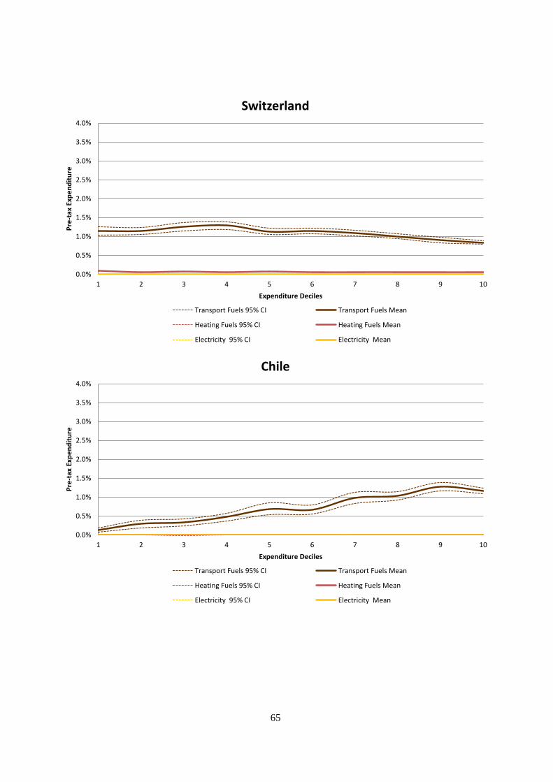
65

0.0%

0.5%

1.0%

1.5%

2.0%

2.5%

3.0%

3.5%

4.0%

1 2 3 4 5 6 7 8 9 10

Pre

-tax

Exp

en

dit

ure

Expenditure Deciles

Switzerland

Transport Fuels 95% CI Transport Fuels Mean

Heating Fuels 95% CI Heating Fuels Mean

Electricity 95% CI Electricity Mean

0.0%

0.5%

1.0%

1.5%

2.0%

2.5%

3.0%

3.5%

4.0%

1 2 3 4 5 6 7 8 9 10

Pre

-tax

Exp

en

dit

ure

Expenditure Deciles

Chile

Transport Fuels 95% CI Transport Fuels Mean

Heating Fuels 95% CI Heating Fuels Mean

Electricity 95% CI Electricity Mean

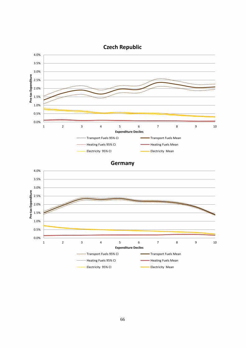
66

0.0%

0.5%

1.0%

1.5%

2.0%

2.5%

3.0%

3.5%

4.0%

1 2 3 4 5 6 7 8 9 10

Pre

-tax

Exp

en

dit

ure

Expenditure Deciles

Czech Republic

Transport Fuels 95% CI Transport Fuels Mean

Heating Fuels 95% CI Heating Fuels Mean

Electricity 95% CI Electricity Mean

0.0%

0.5%

1.0%

1.5%

2.0%

2.5%

3.0%

3.5%

4.0%

1 2 3 4 5 6 7 8 9 10

Pre

-tax

Exp

en

dit

ure

Expenditure Deciles

Germany

Transport Fuels 95% CI Transport Fuels Mean

Heating Fuels 95% CI Heating Fuels Mean

Electricity 95% CI Electricity Mean

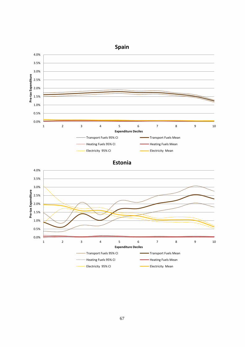
67

0.0%

0.5%

1.0%

1.5%

2.0%

2.5%

3.0%

3.5%

4.0%

1 2 3 4 5 6 7 8 9 10

Pre

-tax

Exp

en

dit

ure

Expenditure Deciles

Spain

Transport Fuels 95% CI Transport Fuels Mean

Heating Fuels 95% CI Heating Fuels Mean

Electricity 95% CI Electricity Mean

0.0%

0.5%

1.0%

1.5%

2.0%

2.5%

3.0%

3.5%

4.0%

1 2 3 4 5 6 7 8 9 10

Pre

-tax

Exp

en

dit

ure

Expenditure Deciles

Estonia

Transport Fuels 95% CI Transport Fuels Mean

Heating Fuels 95% CI Heating Fuels Mean

Electricity 95% CI Electricity Mean

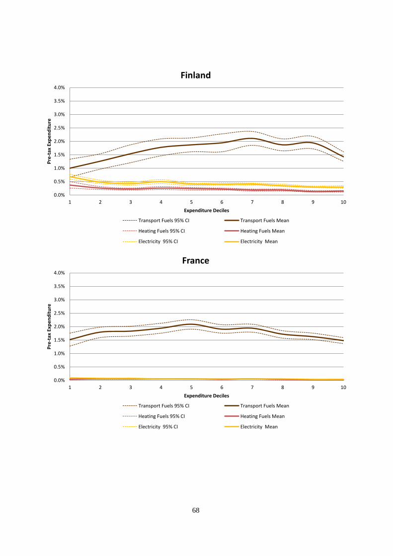
68

0.0%

0.5%

1.0%

1.5%

2.0%

2.5%

3.0%

3.5%

4.0%

1 2 3 4 5 6 7 8 9 10

Pre

-tax

Exp

en

dit

ure

Expenditure Deciles

Finland

Transport Fuels 95% CI Transport Fuels Mean

Heating Fuels 95% CI Heating Fuels Mean

Electricity 95% CI Electricity Mean

0.0%

0.5%

1.0%

1.5%

2.0%

2.5%

3.0%

3.5%

4.0%

1 2 3 4 5 6 7 8 9 10

Pre

-tax

Exp

en

dit

ure

Expenditure Deciles

France

Transport Fuels 95% CI Transport Fuels Mean

Heating Fuels 95% CI Heating Fuels Mean

Electricity 95% CI Electricity Mean

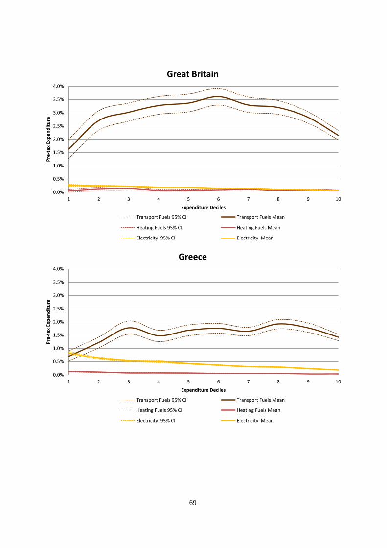
69

0.0%

0.5%

1.0%

1.5%

2.0%

2.5%

3.0%

3.5%

4.0%

1 2 3 4 5 6 7 8 9 10

Pre

-tax

Exp

en

dit

ure

Expenditure Deciles

Great Britain

Transport Fuels 95% CI Transport Fuels Mean

Heating Fuels 95% CI Heating Fuels Mean

Electricity 95% CI Electricity Mean

0.0%

0.5%

1.0%

1.5%

2.0%

2.5%

3.0%

3.5%

4.0%

1 2 3 4 5 6 7 8 9 10

Pre

-tax

Exp

en

dit

ure

Expenditure Deciles

Greece

Transport Fuels 95% CI Transport Fuels Mean

Heating Fuels 95% CI Heating Fuels Mean

Electricity 95% CI Electricity Mean

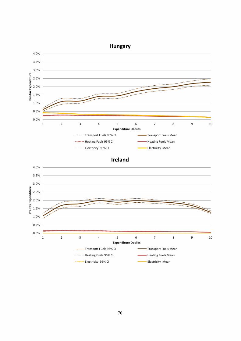
70

0.0%

0.5%

1.0%

1.5%

2.0%

2.5%

3.0%

3.5%

4.0%

1 2 3 4 5 6 7 8 9 10

Pre

-tax

Exp

en

dit

ure

Expenditure Deciles

Hungary

Transport Fuels 95% CI Transport Fuels Mean

Heating Fuels 95% CI Heating Fuels Mean

Electricity 95% CI Electricity Mean

0.0%

0.5%

1.0%

1.5%

2.0%

2.5%

3.0%

3.5%

4.0%

1 2 3 4 5 6 7 8 9 10

Pre

-tax

Exp

en

dit

ure

Expenditure Deciles

Ireland

Transport Fuels 95% CI Transport Fuels Mean

Heating Fuels 95% CI Heating Fuels Mean

Electricity 95% CI Electricity Mean

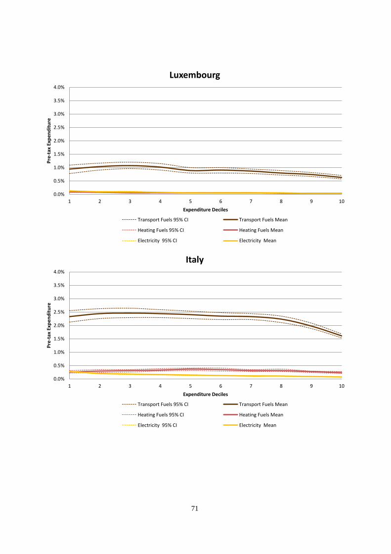
71

0.0%

0.5%

1.0%

1.5%

2.0%

2.5%

3.0%

3.5%

4.0%

1 2 3 4 5 6 7 8 9 10

Pre

-tax

Exp

en

dit

ure

Expenditure Deciles

Luxembourg

Transport Fuels 95% CI Transport Fuels Mean

Heating Fuels 95% CI Heating Fuels Mean

Electricity 95% CI Electricity Mean

0.0%

0.5%

1.0%

1.5%

2.0%

2.5%

3.0%

3.5%

4.0%

1 2 3 4 5 6 7 8 9 10

Pre

-tax

Exp

en

dit

ure

Expenditure Deciles

Italy

Transport Fuels 95% CI Transport Fuels Mean

Heating Fuels 95% CI Heating Fuels Mean

Electricity 95% CI Electricity Mean

72

0.0%

0.5%

1.0%

1.5%

2.0%

2.5%

3.0%

3.5%

4.0%

1 2 3 4 5 6 7 8 9 10

Pre

-tax

Exp

en

dit

ure

Expenditure Deciles

Netherlands

Transport Fuels 95% CI Transport Fuels Mean

Heating Fuels 95% CI Heating Fuels Mean

Electricity 95% CI Electricity Mean

0.0%

0.5%

1.0%

1.5%

2.0%

2.5%

3.0%

3.5%

4.0%

1 2 3 4 5 6 7 8 9 10

Pre

-tax

Exp

en

dit

ure

Expenditure Deciles

Poland

Transport Fuels 95% CI Transport Fuels Mean

Heating Fuels 95% CI Heating Fuels Mean

Electricity 95% CI Electricity Mean

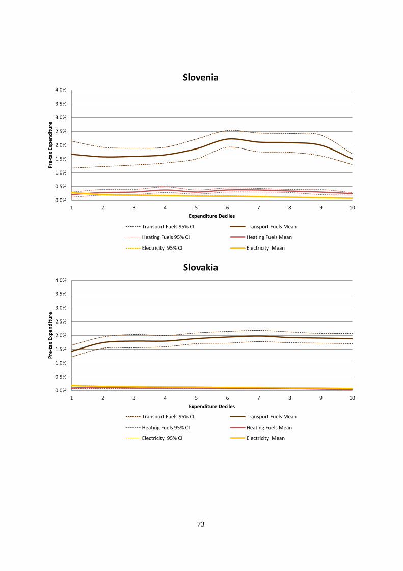
73

0.0%

0.5%

1.0%

1.5%

2.0%

2.5%

3.0%

3.5%

4.0%

1 2 3 4 5 6 7 8 9 10

Pre

-tax

Exp

en

dit

ure

Expenditure Deciles

Slovenia

Transport Fuels 95% CI Transport Fuels Mean

Heating Fuels 95% CI Heating Fuels Mean

Electricity 95% CI Electricity Mean

0.0%

0.5%

1.0%

1.5%

2.0%

2.5%

3.0%

3.5%

4.0%

1 2 3 4 5 6 7 8 9 10

Pre

-tax

Exp

en

dit

ure

Expenditure Deciles

Slovakia

Transport Fuels 95% CI Transport Fuels Mean

Heating Fuels 95% CI Heating Fuels Mean

Electricity 95% CI Electricity Mean

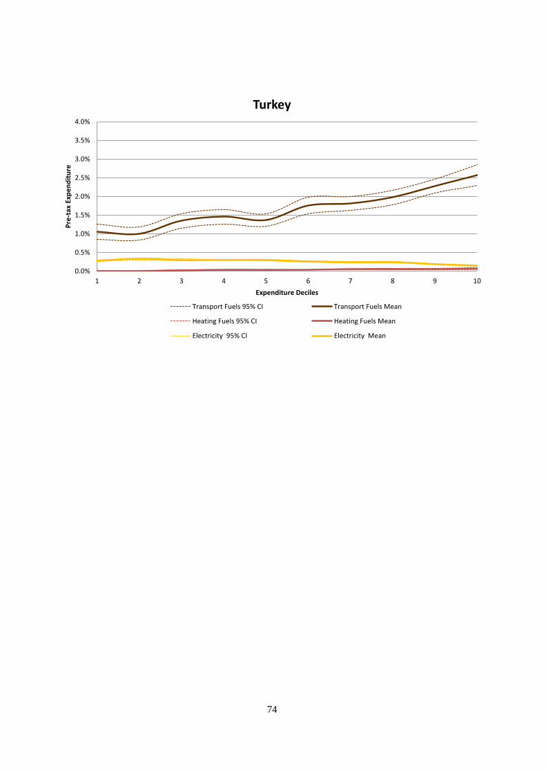
74

0.0%

0.5%

1.0%

1.5%

2.0%

2.5%

3.0%

3.5%

4.0%

1 2 3 4 5 6 7 8 9 10

Pre

-tax

Exp

en

dit

ure

Expenditure Deciles

Turkey

Transport Fuels 95% CI Transport Fuels Mean

Heating Fuels 95% CI Heating Fuels Mean

Electricity 95% CI Electricity Mean