Matching, Sorting, and the Distributional Effects

of International Trade�

Gene M. GrossmanPrinceton University

Elhanan HelpmanHarvard University and CIFAR

Philipp KircherUniversity of Edinburgh

August 2014

Abstract

We study the distributional consequences of trade in a world with two industries and two

heterogeneous factors of production. Productivity in each production unit re�ects the ability of

the manager and the abilities of the workers, with complementarity between the two. We begin

by examining the forces that govern the sorting of worker and manager types to industries, and

the matching of workers and managers within industries. We then consider how changes in

relative output prices generated by changes in the trading environment a¤ect sorting, matching,

and the distributions of wages and salaries. We distinguish three mechanisms that govern the

e¤ects of trade on income distribution: trade increases demand for all types of the factor used

intensively in the export sector; trade bene�ts those types of a factor that have a comparative

advantage in the export sector; and trade induces a re-matching of workers and managers within

both sectors, which bene�ts the more able types of the factor that achieves improved matches.

Keywords: heterogeneous labor, matching, sorting, productivity, wage distribution, inter-national trade.

JEL Classi�cation: F11, F16

�This is a revised version of our working paper Grossman et al. (2013), with the new title better re�ecting thefocus of this article. Part of this research was completed while Grossman was visiting STICERD at the London Schoolof Economics and CREI at the University of Pompeu Fabra and while Helpman was visiting Yonsei University as SKChaired Professor. They thank these institutions for their hospitality and support. The authors are grateful to RohanKekre, Ran Shorrer, Kirill Borusyak, and especially Kevin Lim for their research assistance. Arnaud Costinot, OlegItskhoki, Stephen Redding, Dan Tre�er, Harald Uhlig, Jonathan Vogel, three anonymous referees, and numerousseminar participants provided helpful comments and suggestions. Anders Akerman and Marc-Andreas Muendlergraciously helped with the preparation of data presented in Section 2. Finally, Grossman and Helpman thank theNational Science Foundation and Kircher thanks the European Research Council for �nancial support.

1 Introduction

How does international trade a¤ect a country�s income distribution? This age-old question has been

the subject of a voluminous theoretical literature dating back at least to Ohlin (1933), Haberler

(1936), Viner (1937), and of course Stolper and Samuelson (1941). But, until recently, research

has focused almost exclusively on the relative earnings of a small number of aggregate (or homo-

geneous) factors of production. One can think of this research as addressing the determinants

of �between-occupation� or �between-skill-group�distribution. There has also been a �between-

industry�component to this line of inquiry, as re�ected in the work by Jones (1971), Mayer (1974)

and Mussa (1974) on models with �sector-speci�c�factors of production.

However, between-occupation and between-industry wage variation tell only part of the in-

equality story. Research using household-level data �nds that within occupation-and-industry wage

variation or within skill-group-and-industry variation contributes at least as much as does between-

group variation to the overall level of earnings inequality in the United States, Germany, Sweden,

and Brazil.1 Moreover, changes in within-group distributions account for a signi�cant portion of

the recent trends in wage inequality. While only the research on Brazil attempts to attribute some

of these trends to changes in the trade environment, the evidence of substantial within-group dis-

persion suggests the need for a richer theoretical framework that incorporates factor heterogeneity

in order to help us understand more fully the e¤ects of globalization on income distribution.

In this paper, we introduce factor heterogeneity into a multi-factor model of resource allocation

in order to study the distributional e¤ects of international trade in �ner detail. As in the familiar

Hecksher-Ohlin model, we assume that output is produced by the combined e¤orts of two factors

(or occupations), which we call �workers� and �managers.� These factors are employed in two

competitive industries. But here, the inelastic supply of each factor comprises a continuum of

di¤erent types. Firms form production units that bring together a manager of some type with a

group of workers. There are diminishing marginal returns to adding a greater number of workers

to a team with a given manager, as in the standard model. Meanwhile, the productivity of a unit

depends on the type of the manager and the types of the various workers. Firms must choose not

only how many workers and managers to hire, but also what types to employ. Industries may di¤er

both in their factor intensities (as re�ected in the diminishing returns to workers per manager) and

in the functions that relate productivity to types.

Our model builds not only on Heckscher and Ohlin, but also on Lucas (1978). Lucas assumed

that a �rm�s productivity depends on the ability of its manager (or �entrepreneur�), but that

agents are equally productive qua workers. His analysis focused on the sizes of production units

as a function of the types of their managers, but he could not address the composition of these

units in terms of manager-worker combinations. Eeckhout and Kircher (2012) extended Lucas�s1See, for example, Card et al. (2013) for Germany, Akerman et al. (2013) for Sweden, Helpman (2014) et al. for

Brazil, Mouw and Kalleberg (2010) for the United States, and others.

1

approach to allow for heterogeneity of both factors. Like Lucas, they modeled only a single good-

producing industry and so they could not study the e¤ects of relative output prices on factor

rewards. But they contributed a key result that we borrow here, namely a condition for positive

assortative matching of workers and managers. To apply their insights, we posit the existence of

complementarity between worker ability and manager ability in determining the productivity of

production units in each industry. When these complementarities are strong enough, they imply

that �rms in an industry will combine better managers with better workers.2

In general equilibrium models with homogeneous factors of production, resource allocation can

be fully described by the quantities of every input hired into each sector. With heterogeneous

factors, the assignment of di¤erent types must also be considered. In such a setting, two important

aspects of resource allocation that a¤ect income distribution concern the sorting of heterogeneous

managers and workers to industries and the matching of managers and workers in production units

within each one. Sorting that is guided by comparative advantage generates endogenous sector

speci�city, which partly links workers� and managers� rewards to the prices of the goods they

produce. Endogenous matching creates an additional channel� absent from previous, multi-sector

trade models� through which changes in relative prices can a¤ect the distribution of factor rewards.

If the complementarities between manager and worker ability levels are strong enough to determine

the composition of the production teams that form in general equilibrium, then changes in relative

prices typically induce rematching of managers and workers in each industry. We will be interested

in describing the rematching that results from an improvement in a country�s terms of trade and

in deriving the implications of such changes in the trade environment for within occupation-and-

industry income inequality.3

We are not the �rst to study the implications of sorting and matching for income distribution.

However, previous authors have considered the two forces only in isolation. For example, Ohnsorge

and Tre�er (2007) and Costinot and Vogel (2010) studied the links between trade and income

distribution in an assignment model with heterogeneous workers and many sectors, but with a

linear production function. In this setting, workers sort to sectors, but do not match with any

other factors.4 Yeaple (2005) and Sampson (2014) allow for matching between heterogeneous

workers and �rms that have access to di¤erent technologies. These authors too adopt a linear

production function, but since their �rms produce di¤erentiated products in a world of monopolistic

competition, the hiring of additional labor generates decreasing returns in terms of revenue, and

so they can analyze the sizes of production units. Our model incorporates the forces found in

these earlier papers, but also identi�es a novel and important interplay between matching and

sorting; changes in relative prices generate shifts in the margins of factor sorting, which alter the

2See Garicano and Hubbard (2012) for direct evidence of positive assortative matching between managers andworkers in the U.S. legal services industry and Fox (2009) for indirect evidence of such matching across a range ofU.S. and Swedish industries.

3Krishna et al. (2014) report evidence of an endogenous reassignment of workers to �rms following the Braziliantrade reform of 1991. They conclude based on this evidence that �[e]ndogenous matching of workers with �rms isthus crucial in determining wage outcomes for workers in open economies�(p.252).

4See Ru¢ n (1988) for an antecedent of this approach.

2

composition of types in each industry and so force a rematching of factor types.

In the next section, we revisit the Brazilian data examined by Helpman et al. (2014) in order to

provide some motivating observations for the subsequent theoretical analysis. We �nd a strongly

positive correlation between the mean wage of male workers employed in an industry and the mean

salary of male managers and professionals employed in the same industry, suggestive of positive

assortative matching across industries of worker and manager types. We use this observation later

to guide our emphasis among the various sorting outcomes that can arise in our model. We also �nd

signi�cant changes in within-industry worker and manager earnings distribution over an eight-year

period that spans the major Brazilian trade liberalization of 1991.

In Section 3, we lay out our general equilibrium model of competitive resource allocation with

two heterogeneous factors of production. As already mentioned, the model extends the familiar

Heckscher-Ohlin framework to allow for a continuum of types of both factors. In each of the two

industries, the productivity of a production unit that includes a manager and some endogenously-

chosen number of workers is an increasing, log-supermodular function of the �ability�of the manager

and the ability levels of the associated workers. We take the relative output price as exogenous,

but use it to represent the country�s trading environment.

Section 4 derives the equilibrium conditions for pro�t-maximization, factor-market clearing,

and wage and salary determination. We discuss the equilibrium sorting of workers and managers

to industries, �rst for a case in which productivity is a constant-elasticity function of the ability of

the manager and the abilities of the workers, and then for a case with stronger complementarities,

namely when productivity is a strictly log-supermodular function of the types. In either case,

sorting by each factor is guided by a cross-industry comparison of the ratio of the elasticity of

productivity with respect to ability to the elasticity of output with respect to factor quantity.

When complementarities are strong, the elasticities of productivity with respect to ability re�ect

the matches that take place, and so the sorting by each factor depends on the choices made by

the other factor. After describing the sorting conditions, we de�ne a threshold equilibrium as

one in which sorting of each factor is fully described by a single cuto¤ such that all workers with

ability above the cuto¤ are employed in one industry and the remainder are employed in the other,

and similarly for managers. Several propositions provide su¢ cient conditions for the existence of

a threshold equilibrium, �rst allowing for the possibility that high-ability workers and managers

might not sort to the same sector, but then focusing on an equilibrium with positive assortative

matching across industries.

After characterizing in Section 5 the matches that form between exogenously given sets of worker

types and manager types and discussing how exogenous expansion of these sets induces rematching

that has clear implications for income inequality, we turn in Section 6 to the main task at hand. Here

we ask, how do changes in the trading environment, as re�ected in a country�s terms of trade, a¤ect

earnings inequality between occupations, between industries, and within occupation and industry.

We begin again with the case of constant-elasticity (or Cobb-Douglas) productivity functions, which

generates results that are instructive even if unrealistic. We show that in this environment, an

3

increase in the relative price of a country�s export good generates between-occupation redistribution

that is reminiscent of the Stolper-Samuelson theorem and between-industry redistribution that is

reminiscent of the Ricardo-Viner model with sector-speci�c factors, but it has no a¤ect on within

occupation-and-industry inequality. The complementarities between managers and workers are not

strong enough in the Cobb-Douglas case to determine a unique pattern of matching, and the relative

productivities of di¤erent factor types in an industry are independent of the matches that take place.

With the stronger complementarities that are present when the productivity functions are strictly

log supermodular, the matching pattern in general equilibrium is uniquely determined. Then

endogenous rematching generates predictable changes in within occupation-and-industry income

distributions.

In Section 6.2.1, we consider the distributional e¤ects of price changes in an initial equilibrium in

which the best workers and the best managers sort to opposite sectors. Although this con�guration

seems less empirically relevant than the alternative based on the evidence for Brazil (and also

Sweden), the forces at work are easiest to understand in this case. An increase in the relative price

of the good produced by the higher-ability types of workers and the lower-ability types of managers,

for example, attracts to the industry marginal workers who are less able and marginal managers

who are more able than those who are employed there initially. This results in match upgrading

for all workers initially in the expanding sector and for those who remain in the contacting sector,

which in turn spells a rise in within-occupation-and-industry inequality. The outcome for managers

is just the opposite.

Finally, in Section 6.2.2, we take on the case that probably is most empirically relevant, namely

one in which the most able workers and the most able managers sort to the same industry. We

show that if factor intensities are similar in the two industries, a change in relative price must

increase within-occupation-and-industry inequality for one factor and reduce it for the other. If,

instead, factor intensities di¤er substantially across sectors, then a richer set of outcomes is possible.

For example, an increase in the relative price of the worker-intensive good raises within-industry

inequality among workers in the labor-intensive industry while reducing within-industry inequality

among those in the manager-intensive industry.

Section 7 o¤ers some concluding remarks.

2 Some Motivating Observations

We aim to provide a simple analytical framework that can shed light on the distributional im-

plications of globalization in a world with a broad range of worker types. Our motivation comes

in part from several recent �ndings in the empirical literature on earnings. Researchers such as

Autor et al. (2008) and Kopczuk et al. (2010) have emphasized that trends in income inequality

over the last decade cannot be well summarized by a single summary statistic, such as the relative

wage of skilled versus unskilled workers or the college wage premium. Rather, in several countries,

including the United Stages, inequality has been rising at the top end of the wage distribution, but

4

constant or even declining at the bottom end of the distribution, generating what has been termed

a �hollowing out�of the middle class. Also, Helpman et al. (2014) and Akerman et al. (2013) have

documented that within-industry variation accounts for a large part of the cross-sectional evolution

of wage inequality, even after controlling at a detailed level for workers�occupations. In Brazil,

for example, the authors used a classi�cation system that allows for 12 manufacturing sectors and

more than 300 occupations and found that more than half of the change in wage inequality between

1986 and 1995 occurred within sectors and occupations. Together, these �ndings point to the need

for a framework that allows for multiple worker types and that incorporates links between trade

and relative wages for workers employed in the same occupation and industry.

To set the stage for our theoretical analysis, we draw on the set of linked employer-employee

relationships that were surveyed by the Brazilian Ministry of Labor in its Relação Anual de Infor-

maço�es Sociais (RAIS) and studied previously by Helpman et al. (2014). Our purpose in re-visiting

these data is not to provide a set of targets that will be explained by our theory, but rather to

highlight the rich pattern of outcomes that exist in reality and to establish some stylized facts that

we can use to focus attention among the several �cases�that our model can generate.

We examine distributions of wages and salaries in twelve Brasileiro de Geogra�a e Estatistica

(IBGE) industry categories for the years 1986 and 1994.5 These data represent labor-market

outcomes before and after the major Brazilian trade liberalization of 1991, but before the impact was

felt of the substantial stabilization program that Brazil undertook in 1994. Our model distinguishes

two factors of production that we shall call �managers�and �workers,�and so we compute earnings

distributions in the Brazilian manufacturing industries separately for occupations classi�ed in the

Classi�cação Brasileira de Ocupações Category 1 (professional and managerial labor) and those

in Categories 2-5 (skilled white-collar, unskilled white-collar, skilled blue-collar and unskilled-blue-

collar labor).

In �gure 1, we plot the log of the mean earnings for male managers and professionals in 1994

against the log of the mean wage for male workers, for each of the twelve manufacturing sectors.6

Apparently, the correlation across sectors between the mean earnings of managers and the mean

wage of workers is strongly positive. In our later discussion, we will interpret this positive correlation

to suggest the greater empirical relevance of circumstances in which the more able (and thus higher

paid) managers sort to the same industry as do the more able workers, as compared to circumstances

in which the more able managers sort to the same industry as the less able workers.7 For future

reference, we record

Observation 1 There is a strong positive correlation between the mean wage of male managers

employed in a Brazilian industry and the mean wage of male workers employed in the industry.

5Table 2 includes a list of the industries and their sector numbers.6The plot for wages and salaries in 1986 is qualitatively similar.7Figure A1 in the Appendix plots log of mean wages for Swedish managers and workers in 2004 in 14 manufacturing

industries and shows a similar strong positive correlation. We thank Anders Akerman for computing these meansfrom the Statistics Sweden database that is described in Akerman et al. (2013).

5

Figure 1: Variation across manufacturing industries of log mean salary of male managers and logmean wage of male workers in Brazil, 1994. Source: own calculations.

Male Workers Male Managers

Industry No. 1986 1994 1986 1994

Non-metallic mineral products 2 0.324 0.381 0.308 0.376

Metallic products 3 0.252 0.276 0.219 0.260

Machinery, equipment and instruments 4 0.240 0.266 0.226 0.224

Electrical and telecommunications equipment 5 0.261 0.294 0.203 0.207

Transport equipment 6 0.192 0.236 0.163 0.192

Wood products and furniture 7 0.238 0.331 0.392 0.423

Paper and paperboard, and publishing and printing 8 0.301 0.326 0.319 0.340

Rubber, tobacco, leather and fur 9 0.309 0.344 0.295 0.345

Chemical and pharmaceutical products 10 0.358 0.353 0.247 0.286

Apparel and textiles 11 0.275 0.309 0.347 0.393

Footwear 12 0.259 0.350 0.335 0.349

Food, beverages, and ethyl alcohol 13 0.268 0.345 0.411 0.398

All manufacturing industries 0.318 0.364 0.290 0.329

Table 1: Theil index of inequality by manufacturing industry

6

Table 1 reports the Theil index of income inequality separately for male workers and male

managers and professionals in 1986 and in 1994, for each of the 12 manufacturing industries.8 In

Table 2, we provide two decompositions of the these indexes for each year and for the change

between them. The top part of the table shows a separate decomposition for each occupational

group (i.e., workers and managers) into a component that represents dispersion within industries

and one that represents dispersion between industries.9 The bottom part of the table provides a

decomposition of inequality for all male workers and managers in manufacturing taken together into

components for �within occupation and industry�and �between occupation and industry.�We see

that, in either case, the within component accounts for the largest share of the overall inequality

in each year, as well as the majority of the change that occurred during the period that spanned

the trade reform. We record this �nding in

Observation 2 Within-industry inequality accounts for a majority of the income inequality formale workers and for male managers in Brazil in 1986 and 1994, and for a majority of the

changes in inequality between 1986 and 1994. Within-occupation-and-industry inequality

accounts for a majority of the income inequality for male workers and managers as a group

in 1986 and 1994, and for a majority of the change in inequality between 1986 and 1994.

In Figure 2, we plot the change in the Theil index for workers between 1986 and 1994 against the

change in the Theil index for managers and professionals. The numbers in the �gure again represent

the di¤erent industries, in accordance with the labels provided in Table 2. The �gure reveals a

negative correlation of -0.20 between the changes in inequality for workers and that for managers; in

industries where the spread in the salaries of workers increased greatly, that for managers generally

increased little, or even decreased. We note

8We compute the Theil index of inequality in group k as

Tk =1

Nk

NkXi=1

�yi�yk� ln yi

�yk

�where Nk is the number of individuals in group k, yi is the income of individual i, and �yk is the mean income amongall individuals in group k.

9For a set of groups k = 1; : : : ;K, the overall Theil index is

T =1

N

Xk

Xi

yik�ylnyik�y

where yik is the income of worker i in group k, N =P

kNk and �y is the mean income. We compute the �withincomponent�as

Twithin =Xk

skTk

where sk =Nk �ykN �y

is the income share of group k:The �between component� is

Tbetween =Xk

sk ln�yk�y,

so that T = Twithin + Tbetween.

7

Male Workers Male Managers

1986 1994 Change 1986 1994 Change

Decomposition:

Within/Between Industry

Total inequality 0.318 0.364 0.045. 0.290 0.329 0.039

Within industry 0.272 0.309 0.038 0.262 0.291 0.029

Between industry 0.047 0.054 0.007 0.028 0.038 0.009

Male Workers and Managers

1986 1994 Change

Decomposition:

Within/Between Industry and Occupation

Total inequality 0.423 0.467 0.043

Within occupation and industry 0.269 0.305 0.036

Between occupation and industry 0.154 0.161 0.007

Table 2: Decomposition of income inequality

Figure 2: Correlation across industries of changes in income inequality for Brazilian workers andBrazilian Managers

8

Observation 3 There is a negative correlation across industries between the change in the Theilindex of earnings inequality between 1986 and 1994 for Brazilian workers and the change in

the Theil index of earnings inequality for Brazilian managers.

Finally, in Figure 3, we associate these changes in inequality for each occupational group with

changes in relative prices over the same period. We use wholesale price data (Indice de Precos

por Atacado) computed by Fundação Getulio Vargas (FGV) and a concordance and aggregation

to the twelve IGBE industry categories performed by Marc Muendler.10 The top panel in the

�gure shows that inequality among workers tended to rise in those industries that experienced an

increase in relative price between 1986 and 1994. The correlation coe¢ cient is 0.25. Meanwhile, the

bottom panel in the �gure depicts a negative correlation between the change in the Theil index of

inequality for managers and the evolution of the industry�s relative price. In this case, we compute

the correlation coe¢ cient to be -0.45. We make no claim that these correlations represent causal

links between prices and inequality. Still, it is interesting that industry price changes have an

opposite correlation with changes in inequality for the two factors, which we will �nd is a general

prediction of our model.

Observation 4 The correlation across industries between the change in relative output price andthe change in income inequality between 1986 and 1994 is positive for Brazilian workers and

negative for Brazilian managers.

We o¤er these observations cautiously. For one thing, we have not attempted to isolate the

in�uence of trade liberalization from other forces that may have impacted the wage and salary

distributions in Brazil during the period under consideration. For another, we have not sought to

verify that similar patterns have occurred after trade liberalization or increased exposure to trade in

other countries, especially those with factor endowments similar to those in Brazil. While serious

empirical analysis is beyond the scope of the current paper, the data for Brazil do suggest that

trade impacts di¤erently the earnings of those in an industry and occupation who di¤er in skill and

ability, that within industry-and-occupation redistribution is at least as important as redistribution

between those in di¤erent occupations and industries, that changes in inequality among managers

and workers in an industry are negatively correlated, and that these inequality changes are cor-

related with relative price movements. Finally, the data suggest that greater emphasis should be

placed on parameter con�gurations that imply sorting of the best managers and the best workers

to the same sectors as compared to parameter con�gurations that imply otherwise.

10We begin with the IPA-DI series, which has been used for the Brazilian national accounts since 1944. FGV reportsthese prices at an FGV-speci�c industry level. Muendler used an internal crosswalks made available to him by IBGEto reset those data to the Nivel-100 industry level and then mapped the resulting prices to IGBE subsectors. Heformed aggregates at the 12-industry level of the earnings data using sales data from the 1990 survey of manufacturing�rms (PIA) that is described in Muendler (2004). Finally, we computed price indexes for 1986 and 1994 by averagingthe monthly prices he gave us and constructed relative price changes by dividing the in�ation in each price series bythe average in�ation rate. We are very grateful to Marc Muendler for his assistance in all this.

9

Figure 3: Correlation across industries of changes in income inequality and changes in relativeprices

3 The Economic Environment

We study an economy that produces and trades two goods. This is a �Heckscher-Ohlin economy��

with two factors of production that for concreteness we call �managers� and �workers�� except

that there are many �types� of each factor. The inelastic supplies of the heterogeneous workers

are represented by a density function �L�L (qL), where �L is the aggregate measure of workers in the

economy and �L (qL) is a probability density function (pdf) over worker types, qL. Similarly, the

economy is endowed with a density �H�H (qH) of managers of type qH , where �H is the measure of

managers and �H (qH) is the pdf for manager types. For ease of exposition, we take �L (qL) and

�H (qH) both to be continuous and strictly positive on their respective supports, SL = [qLmin; qLmax]

and SH = [qHmin; qHmax].

We treat factor endowments as exogenous for simplicity, and in order to connect our analysis

with previous studies of trade and factor prices in the spirit of Jones (1965, 1971), Mayer (1974),

Mussa (1974), and others. It might also be interesting to allow for occupational choice, as in

Lucas (1978), or human capital accumulation via education, as in Findlay and Kierzkowski (1983).

Of course, other interpretations of the two factors also are possible. For example, if the factors

are �labor� and �capital,� one presumably would want to incorporate a choice of investment in

machines of di¤erent types, as in Acemo¼glu (1998).

Competitive �rms can enter freely into either industry and access constant-returns-to-scale

technologies. We describe the technology in industry i in terms of the output that can be produced

10

by a manager of some type qH when combined with workers of various types. The manager has an

endogenous �span of control�� as in Garicano (2000) and Eeckhout and Kircher (2012)� inasmuch

as she must allocate her �xed endowment of attention to the various workers placed under her

control. If the productivity of each worker increases with the attention devoted by the manager,

albeit with diminishing returns, then it generically is optimal for the �rm to form production units

that combine a given type of manager with an (endogenous) number of workers of a common type.11

To save on notation, we therefore can describe the technology in sector i in terms of the amount of

potential output xi that can be produced by a unit with one manager of type qH and ` workers of

common type qL, namely

xi = i (qH ; qL) ` i , 0 < i < 1, for i = 1; 2. (1)

Here, i (qH ; qL) re�ects the productivity of the production unit and i is a parameter that

captures the diminishing returns to the size of the workforce that results from an increase in the

manager�s span of control. Since we allow for di¤erent degrees of diminishing returns in the two

sectors ( 1 6= 2), the �rms in di¤erent industries might �nd it optimal to combine a manager with

di¤erent numbers of workers. This gives rise to a possible di¤erence in factor intensities that is

familiar from the traditional Heckscher-Ohlin theory.12 The new element is the productivity term

i (qH ; qL), which is a function of the types of each of the factors. We assume that there exists

an ordering of each factor type such that any change in the type index a¤ects productivity in the

same direction in both industries. Without further loss of generality, then, we can choose the order

so that i (qH ; qL) is strictly increasing in each of its arguments for i = 1 and i = 2. Under this

labeling convention, we refer to qH as the �ability� of the manager and qL as the ability of the

associated workers.

Importantly, we posit the existence of a complementarity between the ability levels of the

manager and the workers that are employed together in a production unit. More able workers are

more productive than less able workers no matter who is their manager, but the more able workers

are assumed to be relatively more productive compared to their less able counterparts when they

are combined with a more able manager rather than a less able manager.13 Formally, we assume

throughout that i (qH ; qL) is strictly increasing and twice continuously di¤erentiable and we adopt

Assumption 1 i (qH ; qL) is log supermodular for i = 1; 2.

Log supermodularity implies that i (q00H ; q

00L) = i (q

00H ; q

0L) � i (q

0H ; q

00L) = i (q

0H ; q

0L) for any q

00H > q0H

11The optimality of combining a given type of manager with workers of a common type arises in other contexts inwhich the manager has a span of control besides the particular description we o¤er here; see Eeckout and Kircher(2012). They show that the key assumption for this result is that there is no teamwork or synergy between workersin the �rm, who interact only insofar as they compete for the manager�s time and attention.12The assumption of a power function for labor� i.e., that the technologies are Cobb-Douglas in factor quantities�

is made for expositional convenience; many of our results do not require this assumption, so long as there are no�factor intensity reversals.�13See, for example, Garicano and Hubbard (2012), who study assignment patterns in the U.S. legal services industry.

They �nd that the more able partners (managers) team with the more able associates (workers) and argue that theirdata are best explained by the existence of complementarity between the managers�and workers�skill or ability.

11

and q00L > q0L. Notice that we allow the two industries to di¤er in the strength of the complementar-

ities between factors, which along with the di¤erences in factor intensities will play an important

role in determining the sorting of the factor types to the two industries.

Much of our analysis will be carried out with a slightly stronger version of our assumption about

complementarities, namely

Assumption 10 i (qH ; qL) is strictly log supermodular for i = 1; 2.

In this case, the weak inequality described in the previous paragraph becomes a strong inequality.

We take all factor markets to be perfectly competitive and frictionless. That is, �rms can

hire managers and workers of any type at salaries r (qH) and wages w (qL) that vary with ability,

of course, but that the individual �rm takes as given. There is no imperfect information about

individuals�abilities, no search costs of any sort, and no unemployment. Adding frictions to the

formation of production units would be an interesting extension, but is beyond the scope of the

current paper.14

As in other models with perfect competition, the impact of the trading environment on local

factor prices is conveyed via relative output prices. For example, the opening of trade from autarky

generates an increase in the relative price of a country�s export good. So does a subsequent improve-

ment in its terms of trade. An import tari¤ raises the relative domestic price of a country�s import

good, except under the conditions of the so-called Metzler paradox (Metzler, 1949). The relative

domestic prices in turn determine the equilibrium wage schedule w (qL) and the salary schedule

r (qH). Accordingly, we can study the e¤ects of changes in the trading environment on the earnings

distribution by considering the comparative static changes in the wage and salary schedules that

result from an arbitrary change in relative prices. There is no need to spell out the foreign supply

conditions, the domestic and foreign demand conditions, or the international equilibrium conditions

for our present purposes.15

4 Sorting and Matching of Managers and Workers

In this section, we lay out the conditions for pro�t maximization and factor-market clearing in

the domestic economy, taking output prices as given. These conditions determine inter alia the

sorting of the di¤erent types of workers and managers to the two industries, the matching of workers

and managers in production units within each sector, and the equilibrium schedules of wages and

salaries. We will characterize the patterns of sorting and matching that can arise in equilibrium

14 In our working paper, Grossman et al. (2013), we allow for directed search by workers in an environment withunemployment generated by search frictions. In that setting, many results have a similar �avor to those derived here,but trade a¤ects the distribution of employment across workers of di¤erent abilities, as well as the distribution ofwages.15 In Grossman et al. (2013) we discuss the determinants of the trade pattern in a world with two countries that

share common homothetic demands and common technologies. We considered countries that di¤er in their aggregateendowments of managers and workers and in their distributions of factor types.

12

and describe some properties of the earnings schedules. Discussion of the responses of wages and

salaries to changes in relative prices is deferred until Section 6 below.

Consider a �rm in sector i that employs a manager of some type qH . This �rm must choose the

type of workers qL and the number of workers ` to combine with the manager, given the output

price and the wage schedule. The �rm�s pro�t, gross of its salary payment to the manager, is given

by

�i (`; qL; qH) = pi i (qH ; qL) ` i � w (qL) ` ,

where pi is the price of good i and w (qL) is the competitive wage paid to a worker with ability qL.

The �rst-order condition with respect to ` yields the conditional labor demand,

` (qL; qH) =

� ipi i (qH ; qL)

w (qL)

� 11� i

, (2)

which is the number of workers the �rm would hire if it were to employ a manager with ability qH ,

choose workers of type qL; and face the wage schedule w (qL).

Next, we substitute ` (qL; qH) into the expression for �i (`; qL; qH) and compute the �rst-order

condition with respect to qL. This yields the �rm�s optimal choice of worker type, given the type

of its manager and taking into account the corresponding size of the optimal production unit. The

�rst-order condition can be written as

"iL(qH ; qL)

i= "w(qL) , (3)

where "iL (qH ; qL) � qL [@ i (qH ; qL) =@qL] = i (qH ; qL) is the elasticity of productivity in sector i

with respect to worker ability and "w(qL) � qL [@w (qL) =@qL] =w (qL) is the elasticity of the wage

schedule. Evidently, the �rm sets the ratio of the elasticity of output with respect to worker ability

to the elasticity of output with respect to worker quantity equal to the elasticity of the wage

schedule.16 The optimal choice of ability re�ects the fact that the �rm has two ways to expand

output, either by hiring better workers or by hiring more workers. The rate at which wages rise

with ability dictates the appropriate trade-o¤ between the two.

Let qL = mi (qH) denote the solution to (3), if the equation has a unique solution. Then mi (qH)

tells us the type of workers that the �rm would combine with a manager of ability qH if it happened

to hire such a manager. For the economy as a whole, the matching function m (qH), if it is well

determined, consists of m1 (qH) for qH 2 QH1 and m2 (qH) for qH 2 QH2, where QHi is the set ofmanagers that is hired in equilibrium in sector i.

Who are the managers that actually are hired into sector i in equilibrium? Were a �rm to

hire a manager with ability qH and pay her the market salary, r (qH), its net pro�t would be

�i (qH) = ~�i (qH)� r (qH), where ~�i (qH) � maxf`;qLg �i (`; qL; qH) is achieved by choosing ` and qL16This condition is analagous to the ones in Costinot and Vogel (2010) and Sampson (2014), except that those

papers have i = 1, because workers are the only factor of production and output is linear in labor quantity. Asecond, heterogeneous factor of production� such as we have introduced here� is necessary to generate re-matchingwithin sectors, which in turn is needed to explain changes in within-occupation-and-industry wage distribution.

13

according to (2) and (3).17 Note that, in a competitive equilibrium, every �rm operating in sector

i breaks even, which implies that �i (qH) = 0 for all qH 2 QHi. Note too that the �rms in sector jshould not be able to make strictly positive pro�ts by hiring the managers that sort in equilibrium

into sector i, or else they would hire these managers instead. This implies that �j (qH) � 0 for allqH 2 QHi, j 6= i. We will return to these zero-pro�t and optimality conditions below.

4.1 Matching and Sorting with Cobb-Douglas Productivity

It is instructive to begin �rst with a special case in which productivity is a constant elasticity

function of the ability of the manager and that of the worker. For this case, we can write

i (qH ; qL) = q�iH q

�iL for i = 1; 2; �i; �i > 0.

For obvious reasons, we shall refer to this as the case of �Cobb-Douglas productivity.�

The Cobb-Douglas productivity function has several special properties that are important in

this context. First, the function is log supermodular, but it is not strictly log supermodular; it

satis�es Assumption 1 but not Assumption 10. Second, the elasticity of output with respect to

worker ability, "iL (qH ; qL), is a constant �i in this case, and independent of both qH and qL.

We can de�ne analogously the elasticity of output with respect to manager ability, "iH (qH ; qL) �qH [@ i (qH ; qL) =@qH ] = i (qH ; qL). This too is a constant, equal to �i, in the case of Cobb-Douglas

productivity.

With "iL = �i, the �rst-order condition (3) for a �rm�s interior choice of worker type in sector i

requires that "w (qL) = �i= i. However, with an arbitrary wage schedule, this condition will only be

satis�ed by a �nite number (possibly only one) of values of qL. Facing such an arbitrary schedule,

all �rms active in an industry would hire one of these �nite number of types. Such choices would

not be consistent with full employment of the continuum of worker types that sorts to an industry.

We conclude that, as a requirement for full employment, the wage schedule must have a constant

elasticity �1= 1 for the range of workers hired into sector 1 and it must have a constant elasticity

�2= 2 for the range of workers hired into sector 2. In other words,

w (qL) = wiq�i= iL for all qL 2 QLi, i = 1; 2; (4)

for some constants, w1 and w2, where QLi is the set of workers hired in sector i. The wage schedule

dictated by (4) makes all �rms operating in industry i indi¤erent between the potential employees

in QLi.

Notice that the wage schedule in (4) leaves �rms in industry i indi¤erent among the potential

employees in QLi no matter what is the type of their manager. Indeed, the Cobb-Douglas produc-

tivity function makes the relative productivity of any two workers independent of manager type. It

follows that matching of workers and managers is not well determined for the case of Cobb-Douglas

17Of course, this statement assumes that (2) has a unique solution; otherwise, the �rm chooses any worker type qLthat maximizes �i along with the corresponding quantity, ` (qL; qH).

14

0.5 0.6 0.7 0.8 0.9 1 1.1 1.2 1.3 1.4 1.50

0.2

0.4

0.6

0.8

1

1.2

1.4

1.6

1.8

qL

w(q

L)

Sector 1 wagesSector 2 wagesSector 1 shadow wagesSector 2 shadow wages

Figure 4: Wage Schedule

productivity; any matches between workers in QLi and managers in QHi can be consistent with

equilibrium, provided that the numbers in all production units are consistent with (2) and the

requirements for aggregate factor-market clearing are satis�ed.

Which workers are employed in industry 1 and which in industry 2? Consider Figure 4, which

depicts the qualitative features of the equilibrium wage schedule for the case in which sL � �1= 1��2= 2 > 0. Once the �wage anchors�, w1 and w2, have been determined in the general equilibrium,

the solid curve in the �gure represent the equilibrium wage schedule that satis�es (4). The broken

curves show what the wages for di¤erent types of workers would have to be in order to make the

�rms in an industry indi¤erent between hiring these types and the types that are actually employed

in equilibrium. The fact that �1= 1 > �2= 2 implies that the solid curve lies above the broken

curve for industry 2 to the right of the point of intersection, q�L, and that the solid curve lies above

the broken curve for industry 1 to the left of the intersection point. In equilibrium, the �rms in

industry 1 are willing to hire any workers with ability above q�L, but not those with ability below

this level. Meanwhile, the �rms in industry 2 are willing to hire any workers with ability below q�L,

but not those with ability above this level. Evidently, those with ability above q�L sort to industry

1 and those with ability below q�L sort to industry 2, and the marginal workers with ability equal to

q�L are paid the same wage by both sectors. Sorting of workers is guided by sL, the cross-industry

comparison of the ratio of the elasticity of productivity with respect to ability to the elasticity of

output with respect to quantity.

What about the managers? In the appendix we show that the zero pro�t condition, �i (qH) = 0

for all qH 2 QHi, together with (2), (3) and (4), imply that

r (qH) = riq�i=(1� 1)H for all qH 2 QHi, i = 1; 2; (5)

where ri is a constant analogous to wi.18 Then the condition that �j (qH) � 0 for all qH 2 QHi,

18The constants, w1 and w2, are determined along with q�L by a pair of labor-market clearing conditions for the

15

j 6= i; (i.e., that �rms do not want to hire the managers employed in the opposite sector) dictates

the sorting pattern for managers: If sH � �1= (1� 1) � �2= (1� 2) > 0, then managers with

ability above some cuto¤ q�H sort to sector 1 and those with ability below q�H sort to sector 2;

otherwise, the sorting pattern is just the opposite. Notice that the sorting pattern for managers

can be understood similarly to that for workers. Constant returns to scale implies that the elasticity

of output with respect to the number of managers in sector i is 1� i. So, the sorting of managersis guided by a cross-industry comparison of the ratio of the elasticity of productivity with respect

to manager ability to the elasticity of output with respect to the number of managers.19

The case of Cobb-Douglas productivity generates what we will call a threshold equilibrium; the

sorting pattern in general equilibrium is characterized by a pair of boundary points, q�L and q�H ,

such that all workers with ability above q�L sort to some sector and all workers with ability below

q�L sort to the other, and similarly all managers with ability above q�H sort to some sector while

those with ability below q�H sort to the other.20 We note for future reference that there are two

possible types of threshold equilibrium that can emerge. If sL and sH share the same sign, then

the most able workers and the most able managers sort to the same sector. We will refer to this

below as an HH=LL equilibrium, to convey that the �high types�of both factors sort together, as

do the �low types.�Alternatively, if sL and sH are opposite in sign, then the more able managers

sort to the same sector as the less able workers. We will refer to such an outcome as an HL=LH

equilibrium. Recall Observation 1 in Section 2, which suggests that the HH=LL equilibrium may

be the more empirically relevant of the two.

4.2 Matching and Sorting with Strictly Log Supermodular Productivity

Armed with an understanding of the knife-edge case of Cobb-Douglas productivity, we turn to

a case with stronger complementarities between manager and worker abilities that arises under

Assumption 10.

When the productivity function i (qH ; qL) for i = 1; 2 is strictly log supermodular, the argu-

ments presented in Eeckhout and Kircher (2012) imply positive assortative matching (PAM) in each

industry. That is, among the workers and managers that sort to any industry, the better workers

are teamed with the better managers. This is true, because the productivity of a group of more

able workers relative to that of a group of less able workers is higher when the groups are combined

with a more able manager compared to when they are combined with a less able manager. As we

shall see, the equilibrium may or may not exhibit PAM for the economy as a whole.

In the appendix, we show that the solution to the �rms�pro�t maximization problem and the

requirements for factor-market clearing together generate equilibrium allocation sets QLi and QHi

two sectors (which are provided in the appendix) and the requirement that the wage function is continuous at q�L;i.e., w1 (q�L)

�1= 1 = w2 (q�L)

�2= 2 . Given w1 and w2, the salary anchors r1 and r2 are readily calculated.19We do not consider the non-generic situations that arise when sL = 0 or sH = 0, in which case the heterogeneous

workers or managers would be indi¤erent as to their choice of sector.20For some prices, there may be complete specialization in one sector or the other, in which case q�L = qLmin

or q�L = qLmax and q�H = qHmin or q�H = qHmax. In such cases, marginal changes in prices have no e¤ect on theequilibrium, and so they are uninteresting for our purposes. We do not consider them any further.

16

that are unions of closed intervals. (A threshold equilibrium is the special case in which each QFifor F = H;L and i = 1; 2 is a single closed interval.)

Recall now that mi (qH) is the common ability level of the workers who would be teamed with

a manager of ability qH if that manager happened to be employed in sector i. The equilibrium

matching function for the economy, which we denoted by m (qH), consists of m1 (qH) for qH 2 QH1and m2 (qH) for qH 2 QH2. The matching function generates a pair of closed graphs,

Mi = [fqH ; qLg j qL 2 mi (qH) for all qH 2 QHi] , i = 1; 2,

where Mi represents the production units that form in sector i in equilibrium. These graphs

comprise a union of connected sets Mni , i.e., Mi = [n2NiMn

i , such that mi (qH) is continuous and

strictly increasing in each set but may jump discontinuously between them. The fact that mi (qH)

is strictly increasing in each set is a re�ection of PAM.

We prove in the appendix that the equilibrium wage schedule is di¤erentiable everywhere and

use the notation for the matching function to rewrite (3) slightly as

"iL [qH ;m (qH)]

i= "w [m (qH)] for all fqH ;m (qH)g 2Mn;int

i , i = 1; 2; (6)

where Mn;inti is the interior of the set Mn

i . This way of expressing a �rm�s optimal choice of

workers given the identity of the manager emphasizes the fact that the elasticity of productivity

with respect to worker ability depends upon the particular matches between workers and managers

that actually form in equilibrium. These matches in turn re�ect the sorting patterns of workers

and managers to industries.

Using (2) and (3), the zero-pro�t condition �i (qH) = 0 for all qH 2 QHi can be written now as

r (qH) = i

1� ii (1� i) p

11� ii i [qH ;m (qH)]

11� i w [m (qH)]

� i1� i for all qH 2 QHi; i = 1; 2: (7)

This equation and (6) imply that

"iH [qH ;m (qH)]

1� i= "r (qH) for all fqH ;m (qH)g 2Mn;int

i ; i = 1; 2; (8)

where "r(qH) � qH [@r (qH) =@qH ] =r (qH). Notice the similarity with (6); pro�t maximization and

zero pro�ts ensure that the ratio of the elasticity of productivity with respect to manager ability to

the elasticity of output with respect to manager quantity is equal, in equilibrium, to the elasticity of

the salary schedule. But, as with workers, the elasticity of productivity with respect to (manager)

ability depends on the matches that take place.

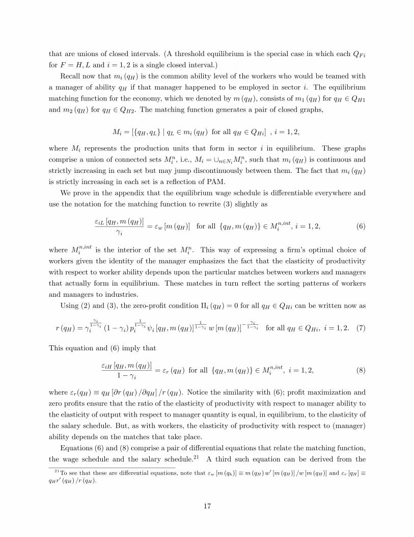
Equations (6) and (8) comprise a pair of di¤erential equations that relate the matching function,

the wage schedule and the salary schedule.21 A third such equation can be derived from the

21To see that these are di¤erential equations, note that "w [m (qh)] � m (qH)w0 [m (qH)] =w [m (qH)] and "r [qH ] �

qHr0 (qH) =r (qH).

17

requirements for factor-market clearing. To this end, consider any connected set of managers

[qHa; qH ] that sorts to industry i and the set of workers qL 2 [m (qHa) ;m (qH)] with whom these

managers are matched in equilibrium. A pro�t-maximizing �rm in sector i that employs a manager

with ability qH and workers of ability qL hires ir (qH) = (1� i)w (qL) workers per manager. Sincethe matching function is everywhere increasing, it follows that

�H

Z qH

qHa

ir (q)

(1� i)w [m (q)]�H (q) dq = �L

Z m(qH)

m(qHa)�L [m (q)] dq ;

where the left-hand side is the measure of workers hired collectively by all �rms operating in sector

i that employ managers with ability between qHa and qH and the right-hand side is the measure

of workers available to be teamed with those managers. Since the left-hand side is di¤erentiable

in qH as long as qH is not a boundary point between managers that sort to di¤erent industries,

this equation implies that the matching function m (qH) also is di¤erentiable at such points. That

being the case, we can di¤erentiate the labor-market clearing condition with respect to qH to derive

a di¤erential equation for the matching function, namely

�H ir (qH)

(1� i)w [m (qH)]�H (qH) = �L�L [m (qH)]m

0 (qH) for all fqH ;m (qH)g 2Mn;inti ; i = 1; 2 .

(9)

This condition states that the workers demanded by a (small) set of managers with ability in a small

range around qH equals the density of workers in the economy that match with these managers.

At last, we are in a position to characterize an equilibrium allocation for the economy, given

prices. Such an allocation is fully described by a quadruple of sets, QiF for F = H;L and i = 1; 2,

a continuous wage schedule w (qL), a continuous salary schedule r (qH) and a piecewise continuous

matching function m (qH) that satisfy the di¤erential equations (6), (8) and (9) and that yield zero

pro�ts per (7) for any active sector (and non-positive pro�ts for any inactive sector).

The sorting patterns in this economy can in principle be quite complex. We wish to identify

conditions that ensure a simple pattern� in particular, a threshold equilibrium� which, as we have

seen, is the pattern that always emerges in an economy with Cobb-Douglas productivity functions.

To motivate our �rst proposition, recall Figure 4. The �gure shows the wage function and shadow

wage functions that result with Cobb-Douglas productivity. To the right of the cuto¤, q�L, the �rms

in industry 1 are willing to pay the (high-ability) workers more than �rms in industry 2, because

the ratio of the elasticity of productivity with respect to worker ability to the elasticity of output

with respect to number of workers, "iL= i = �i= i, is higher there. Similarly, to the left of q�L, it

is industry 2 that is willing to pay the (low-ability) workers more, because "iL= i is lower there.

The wage and shadow-wage functions re�ects these elasticity ratios at each point in the ability

distribution.

The wage and shadow-wage functions also re�ect these elasticity ratios in an economy with

strictly log supermodular productivity functions; see (3). A potential complication arises, however,

because the elasticity ratio for a worker depends upon the identity of the manager with whom

18

the worker is matched, which in turn depends upon the incentives for sorting that confront the

managers. But suppose that the elasticity ratio in industry 1 is higher than in industry 2, even if in

the former case the workers of some ability level are teamed with the economy�s least able manager

and in the latter case they are teamed with the economy�s most able manager. Considering the

complementarity between worker and manager ability levels, the elasticity ratio in industry 1 for a

given worker then must be higher than that in industry 2 for the matches that actually take place,

no matter what they happen to be. These circumstances ensure the existence of a cuto¤ ability

level for workers q�L such that �rms in industry 1 are willing to pay workers with ability above q�L

more than industry 2, and the opposite is true for workers with ability less than q�L� for much the

same reasons as in the case of Cobb-Douglas productivity. In the appendix, we formally prove

Proposition 1 Suppose that Assumption 10 holds and that

"iL (qHmin; qL)

i>"jL (qHmax; qL)

j

for all qL 2 SL; i 6= j; i 2 f1; 2g. Then, in any competitive equilibrium with employment of

workers in both sectors, the more able workers with qL > q�L are employed in sector i and the less

able workers with qL < q�L are employed in sector j, for some q�L 2 SL.

We have seen for the case of Cobb-Douglas productivity that an analogous condition that

compares elasticity ratios across sector guides the sorting of managers. Speci�cally, whichever

industry has the higher ratio of the elasticity of productivity with respect to manager ability to

the elasticity of output with respect to manager quantity attracts the more able managers. Again,

with a general, strictly log supermodular productivity function the sorting incentives for the other

factor (workers, in this case) can complicate this comparison of elasticity ratios. But, in analogy

to Proposition 1, they will not do so if the forces attracting the more able managers to sort to a

sector would remain active even if the match there were consummated with the economy�s least

able workers and the match in the other sector were consummated with the economy�s most able

workers. We record

Proposition 2 Suppose that Assumption 10 holds and that

"iH (qH ; qLmin)

1� i>"jH (qH ; qLmax)

1� j

for all qH 2 SH ; i 6= j; i 2 f1; 2g. Then, in any competitive equilibrium with employment of

managers in both sectors, the more able managers with qH > q�H are employed in sector i and the

less able managers with qH < q�H are employed in sector j, for some q�H 2 SH .

Clearly, if the inequality in Proposition 1 holds for some i and j and the inequality in Proposition

2 also holds for some i0 and j0, then the outcome is a threshold equilibrium. As with the case of

Cobb-Douglas productivity, such an equilibrium can take one of two forms. If i = i0 and j = j0,

19

then the more able workers sort to the same sector as the more able managers, which characterizes

an HH=LL equilibrium. Alternatively, if i = j0 and j = i0, then the more able workers sort to the

opposite sector from the more able managers, which de�nes an HL=LH equilibrium.

It is possible to provide a weaker su¢ cient condition for the existence of a threshold equilibrium

of the HH=LL variety. If the most able managers sort to industry 1, this can only strengthen the

incentives for the most able workers to sort there too in light of the complementarities between

factor types. Similarly, if the most able workers sort to industry 1, this will strengthen the incentives

for the most able managers to do so as well. This reasoning motivates the following proposition

(proven in the appendix), that has less stringent conditions for the emergence of an HH=LL

threshold equilibrium.

Proposition 3 Suppose that Assumption 10 holds. If

"iL (qH ; qL)

i>"jL (qH ; qL)

jfor all qH 2 SH ; qL 2 SL;

and"iH (qH ; qL)

1� i> jH (qH ; qL)

1� jfor all qH 2 SH ; qL 2 SL;

for i 6= j, i = 1 or i = 2, then in any competitive equilibrium with employment of managers and

workers in both sectors, the more able managers with qH > q�H and the more able workers with

qL > q�L are employed in sector i; while the less able managers with qH < q�H and the less able

workers with qL < q�L are employed in sector j, for some q�H 2 SH and some q�L 2 SL.

The di¤erence in the antecedents in Propositions 1 and 2 on the one hand and in Proposition

3 on the other is that, in the former, we compare the elasticity ratio for each factor when it is

combined with the least able type of the other factor in one sector versus the most able type

in the other sector, whereas in the latter we compare the elasticity ratios for common partners

in the two sectors. The di¤erence arises, because an HH=LL equilibrium has PAM within and

across industries, whereas an HL=LH equilibrium has PAM only within industries. In an HL=LH

equilibrium, an able manager in sector i might be tempted to move to sector j despite a generally

greater responsiveness of productivity to ability in i, because the better workers have incentive to

sort to j, and with log supermodularity of j (�), the able manager stands to gain most from this

superior match. In contrast, in an HH=LL equilibrium, the able manager in sector i would �nd

less able workers to match with were she to move to sector j, so the temptation to switch sectors

in order to upgrade partners is not present.

We have provided su¢ cient conditions for the existence of a threshold equilibrium in which the

allocation set for each factor and industry comprises a single, connected interval. These conditions

are not necessary, however, because the matches available to types that are quite di¤erent from the

marginal type might not overturn their strong comparative advantage in one sector or the other.

Nonetheless, not all parameter con�gurations give rise to equilibria with such a simple sorting

20

1 1.1 1.2 1.3 1.4 1.5 1.6 1.7 1.8 1.9 21

1.01

1.02

1.03

1.04

1.05

1.06

1.07

1.08

1.09

1.1

qL

q H

Sector 1Sector 2

Figure 5: Matching: The most and least able workers and the most able mangers sort into sector 1

pattern. An example of a more complex sorting pattern is illustrated in Figure 5.22 The �gure

shows, for each worker type indicated along the horizontal axis, the sector in which that worker

is employed and the type of the manager with whom he is matched. In this example, the most

able and least able workers sort to sector 1 while an intermediate interval of worker types sort to

sector 2. The �rms in sector 1 hire the economy�s most able managers whereas those in sector

2 hire those with ability below some threshold level. Notice that graphs M1 and M2 display the

general properties that we described above; they are unions of connected sets, with a matching

function m(qH) that is continuous and increasing within any such set. The �gure re�ects a �sorting

reversal� for workers that arises because the elasticity ratio for labor is higher in sector 1 when

worker ability is low or high, but higher in sector 2 for a middle range of abilities. Of course, other

sorting patterns besides that depicted in Figure 5 also are possible.

5 Matching and Earnings within Groups

Before we turn to the e¤ects of changes in the trade environment on the distributions of wages

and salaries, it will prove useful to examine in some detail the implications of our equilibrium

conditions for the particular matches that form among a group of workers and a group of managers

that happen to be combined in equilibrium, and for the distributions of wages and salaries in the

two groups. To this end, consider a group of managers comprising all those with ability in the

interval QH = [qHa; qHb] and a group of workers comprising all those with ability in the interval

QL = [qLa; qLb]. Suppose these two groups happen to sort to some industry i in a competitive

equilibrium and that, collectively, the managers and workers in these two groups happen to be

matched together, exhaustively. We are interested in the properties of the solution to the system

of di¤erential equations comprising (6), (8) and (9) along with the zero-pro�t condition, (7), and

the two boundary conditions, qLa = mi (qHa) and qLb = mi (qHb). Throughout this section, we

22The functional forms and parameter values underlying this example are presented in Lim (2013).

21

Lq

Hq

b

a

'b

)( Hqm

Figure 6: Shift in the matching function when qLb rises to qLb0 .

assume the existence of strong complementarities between worker and manager types; i.e., we take

productivity to be a strictly log supermodular function of the two ability levels, as embodied in

Assumption 10.

In the appendix, we prove that the solution has several notable properties. First, if the price piwere to rise without any change in the composition of the two groups, then the matches between

particular members of the groups would remain unchanged and all wages and salaries would rise

by the same proportion as the output price. Second, if the number of managers in QH were to

increase by some proportion h relative to the number of workers in QL, without any change in

the relative densities of the di¤erent types, then the wages of all workers in QL would rise by the

proportion (1� i)h, while the salaries of all types in QH would fall by the proportion ih. Again,there would be no change in the matching between manager and worker types.

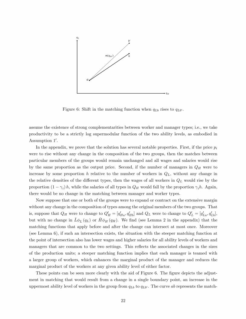
Now suppose that one or both of the groups were to expand or contract on the extensive margin

without any change in the composition of types among the original members of the two groups. That

is, suppose that QH were to change to Q0H = [q0Ha; q

0Hb] and QL were to change to Q

0L = [q

0La; q

0Lb],

but with no change in �L�L (qL) or �H�H (qH). We �nd (see Lemma 2 in the appendix) that the

matching functions that apply before and after the change can intersect at most once. Moreover

(see Lemma 6), if such an intersection exists, the situation with the steeper matching function at

the point of intersection also has lower wages and higher salaries for all ability levels of workers and

managers that are common to the two settings. This re�ects the associated changes in the sizes

of the production units; a steeper matching function implies that each manager is teamed with

a larger group of workers, which enhances the marginal product of the manager and reduces the

marginal product of the workers at any given ability level of either factor.

These points can be seen more clearly with the aid of Figure 6. The �gure depicts the adjust-

ment in matching that would result from a change in a single boundary point, an increase in the

uppermost ability level of workers in the group from qLb to qLb0 . The curve ab represents the match-

22

ing that takes place between the initial groups of workers and managers, whereas ab0 represents the

matching of the same set of managers with the broader set of workers. Naturally, the two curves

have a point in common, at a; PAM ensures that the managers with ability qHa match with the

workers of ability qLa in both circumstances. By Lemma 2 in the appendix, the two curves can have

at most one point in common, so there can be no further points of intersection. That is, the new

matching function ab0 must lie uniformly above ab to the right of point a. In the new equilibrium

with a broader (and better) group of workers, every manager in QH with ability greater than qHaachieves a better match than before. Meanwhile, every worker with ability greater than qLa but

less than or equal to qLb pairs with a less able manager than before. Finally, Lemma 6 implies that

salaries rise for all managers in QH , while wages fall for all workers in QL.

The adjustment in matching that is illustrated in Figure 6 also has implications for within-

group inequality. Consider the wage distribution among workers in QL. The di¤erential equation

(6) implies that

lnwi (qLc)� lnwi (qLc0) =Z qLc0

qLc

iL [�i (x) ; x]

i i [�i (x) ; x]dx; for all qLc;qLc0 2 QL ; (10)

where �i (�) is the inverse of mi (�). If follows that, if all workers with ability levels between qLcand qLc0 , qLc > qLc0 , are teamed with less able managers than before, the wage of the more able

worker of type qLc declines relative to that of the less able worker of type qLc0 . The downgrading

of managers is detrimental to both of these workers, but the strong complementarity between

factor types means that it is especially so to the more able of the pair. Speci�cally, strict log

supermodularity of i (qH ; qL) implies that iL (qH ; qL) = i (qH ; qL) is a strictly increasing function

of qH . It follows that a rematching of a group of workers with less able managers, as depicted in

Figure 6, generates a narrowing of wage inequality within the group QL.23 By a similar argument

(and using the di¤erential equation (8) for salaries), the rematching depicted in Figure 6 generates

a spread in the salary distribution for managers in QH inasmuch as these managers all see their

matches improve.

Similar reasoning can be used to describe the shift in the matching function� and the wage and

salary responses� for changes in the other boundary points. For example, if the lower boundary of

the interval of managers rises from qHa to qHa0 , the matching function shifts downward (thereby

connecting a point to the right of a in Figure 6 with point b), and thus the manager types that

remain in the sector �nd that their matches deteriorate while all workers in QL match with better

managers than before. Such a rematching narrows the salary distribution, while exacerbating wage

inequality.

In short, whenever the matches improve for a group of workers employed in some sector, they

deteriorate for the managers there, and vice versa. As a result, within-occupation-and-industry

inequality among workers and managers tend to shift in opposite directions. This implication of

23Costinot and Vogel (2010) and Sampson (2014) �nd similar results for wage inequality when workers downgradetheir matches with �rms that di¤er in technological sophistication.

23

our model gives it the potential to rationalize Observation 3 in Section 2, namely that changes in

inequality among Brazilian workers and managers are negatively correlated across industries.

6 The E¤ects of Trade on Earnings Inequality

We come �nally to the main concern of our analysis: How does trade a¤ect the distribution of income

within and between occupations and industries? We study the e¤ects of trade by examining the

comparative statics with respect to output prices. In a world of competitive industries, an opening

of trade induces an increase in the relative price of a country�s export good. An expansion of trade

opportunities that improves a country�s terms of trade does likewise. So too does a reduction in a

country�s import tari¤ or other trade barriers, except under the conditions for the Metzler paradox.

So, we can study the e¤ects of trade without introducing the details of other countries by simply

investigating how output prices feed through to factor markets.24

To preview what lies ahead, we will identify and describe three forces that are at work in this

setting. Two are familiar and one is new. First, whenever 1 6= 2, our model features factor

intensity di¤erences across industries. As is well known from the Stolper-Samuelson theorem,

this consideration introduces an e¤ect of trade on between-occupation distribution; an increase in

the relative price of a good tends to increase demand for all types of the factor used intensively

in producing that good, while reducing the demand for all types of the other factor. Second,

our model incorporates factor heterogeneity that, whenever 1 (�) 6= 2 (�), generates comparativeadvantage for certain types of each factor in one industry or the other. This feature introduces an

e¤ect of trade on between-industry distribution; an increase in the relative price of a good tends

to increase the rewards for all types of both occupations that enjoy a comparative advantage in

producing that good, and to reduce the returns to types that hold a comparative disadvantage

in doing so. This e¤ect is familiar from the Ricardo-Viner model with sector speci�city. Finally,

whenever i (qH ; qL) exhibits strict log supermodularity, our model determines the matches that

form between managers and workers in each industry. This feature introduces an e¤ect of trade on

within-group (occupation-and-industry) distribution.

6.1 Wages and Salaries with Cobb-Douglas Productivity

As before, it is instructive to begin with the knife-edge case in which productivity in each sector

is log supermodular, but not strictly so. We revisit an economy with Cobb-Douglas productivity;

i.e., i (qH ; qL) = q�iH q

�iL for i = 1; 2; �i; �i > 0.

Recall from Section 4.1 that, with Cobb-Douglas productivity in each sector, the sorting of fac-

tors to sectors is guided by a cross-industry comparison of the ratio of the elasticity of productivity

with respect to a factor�s ability to the elasticity of output with respect to factor quantity. That

24 In our working paper, Grossman et al. (2013), we link the pattern of trade to cross-country di¤erences inquantities and distributions of the two factors. Thus, we treat the the price change that results from an opening oftrade as an endogenous re�ection of factor-endowment di¤erences. Here, we take the price changes as exogenous inorder to focus attention on the distributional implications of changes in the trade environment.

24

is, when �i= i > �j= j , higher ability confers a comparative advantage among workers for employ-

ment in industry i, while when �i0= (1� i0) > �j0=�1� j0

�, higher ability confers a comparative

advantage among managers for employment in industry i0. The matches that form between workers

and managers that sort to an industry are indeterminate.

It is clear from (4) and (5) that trade has no e¤ect on within-group inequality in these cir-

cumstances. The relative wage of any two workers with ability levels qLa and qLb that are both

employed in the same sector i before and after any change in the trading environment is fully deter-

mined by their relative ability levels; i.e., w (qLa) =w (qLb) = (qLa=qLb)�i= i . Similarly, the relative

salary of any two managers with ability levels qHa and qHb that are employed in sector i prior

and subsequent to a change in the trading environment is r (qHa) =r (qHb) = (qHa=qHb)�i=(1� i).

Evidently, the complementarity between factor types must be strong enough to induce endogenous

meaningful rematching, or else relative wages within any occupation-and-industry group will be

�xed by technological considerations and una¤ected by trade.

The e¤ects of trade on between-occupation and between-industry inequality can be seen from

the comparative-static responses of the wage anchors, w1 and w2, and the salary anchors, r1 and

r2. These comparative statics can be computed from six equations that also determine q�L and q�H :

two equations that ensure that the demand for workers that sort to each sector equals the supply of

workers that does so; two equations that ensure that the wage and salary schedules are continuous

at q�L and q�H , respectively; and two equations that ensure that pro�ts are zero in each industry.

The equations and calculations are provided in the appendix.

The Ricardo-Viner and Stolper-Samuelson forces can be seen most clearly in certain limiting

cases. Suppose, for example, that 1 � 2; i.e., there are only small cross-industry di¤erences in

the diminishing returns to the number of workers per manager and thus small di¤erences in the

intensity of factor use. In this case, if �i > �j , then an increase in the price ratio pi=pj generates

an increase in wi relative to wj and if �i0 > �j0 , an increase in pi0=pj0 generates an increase in ri0

relative to rj0 . Consider for example the e¤ect of the price change on workers. With i � j , the

fact that �i > �j implies that high-ability workers have a comparative advantage in sector i relative

to sector j, and vice versa for low-ability workers. Then, if the relative price of good i increases,

this changes the between-industry distribution, favoring those (high-ability workers) employed in

sector i relative to those (low-ability workers) employed in sector j. An analogous explanation

applies to the changes in the between-industry distribution of managerial salaries.

Now suppose that i > j , whereas �1= 1 � �2= 2 and �1= (1� 1) � �2= (1� 2). Withthis constellation of parameters, the forces that give certain types of each factor a comparative

advantage in one sector or the other are muted. No matter what sorting pattern emerges, the

predominant e¤ect of trade will be on the between-occupation distribution. In particular, since

sector i makes relatively intensive use of workers and sector j makes relatively intensive use of

managers, an increase in pi=pj increases both wi and wj relative to both ri and rj . All workers

gain relative to all managers. Indeed, we can go further to say� as an extension of the Stolper-

Samuelson theorem� that when i > j , an increase in the relative price of good i raises the real

25

income of every type of worker and reduces the real income of every type of manager.

Another instructive case has i � j and �1 � �2, but �i > �j . Then, there is little di¤erence in

factor intensity and little di¤erence in the relative productivity of managers of di¤erent abilities in

the two sectors. What remains is a strong tendency for the high-ability workers to sort to industry i

and the low-ability workers to sort to industry j, in accordance with their comparative advantages.

This is a case where the workers have industry speci�city, but the managers do not (or only slightly

so). As in the classic Ricardo-Viner model (e.g., Jones, 1971), we �nd that when pi=pj rises, the

real incomes of all (high-ability) workers who start in industry i increase while the real incomes of

all (low-ability) workers who end up in industry j fall. In other words, trade bene�ts the worker

types that have speci�city in the export sector but harms the worker types that have speci�city in

the import-competing sector.25 In contrast, trade has a qualitatively similar impact on all manager

types; their real salaries rise in terms of good i but fall in terms of good j.

In less extreme cases, the Stolper-Samuelson and Ricardo-Viner forces coexist. We �nd that

the worker types with comparative advantage in industry i always gain relative to those with

comparative advantage in industry j when the relative price of good i rises. Similarly, the manager

types that sort to industry i gain relative to those that sort to industry j. Whether a group of

workers or a group of managers bene�ts absolutely, and not just relatively, from a change in the trade

environment depends on the direction and strength of the Stolper-Samuelson forces; for example,

all workers may gain from an increase in pi=pj if industry i is much more labor intensive than

industry j, whereas only some may gain if the di¤erence in factor intensity is smaller, and all may

lose if the factor-intensity ranking runs in the opposite direction. These �ndings are reminiscent of

those described by Mussa (1982) for an economy with �imperfect factor mobility�and by Grossman

(1983) for an economy with �partially mobile capital.�

The results described in this section are interesting and will help us to understand those that

follow. But they are not consistent with the evidence presented in Section 2, in particular because

they imply that trade has no e¤ect on within occupation-and-industry earnings inequality. We have

noted, for example, that within-group variation accounted for a majority of the overall change in

Brazilian income inequality that occurred during the period that spanned the trade liberalization

of 1991. To allow for changes in within-group inequality, we must re-introduce Assumption 10.

6.2 Wages and Salaries with Strictly Log Supermodular Productivity

We henceforth assume that productivity in each sector is a strictly log supermodular function of

the ability of the manager and the abilities of the workers; i.e., we adopt Assumption 10. We shall

limit our attention to threshold equilibria; i.e., those that can be characterized by a pair of cuto¤

points, q�L and q�H ; such that all workers with ability above the cuto¤ sort to one industry and all

those with ability below the cuto¤ sort to the other, and similarly for managers.

25 If we instead assume that i > j and that �i= i > �j= j , but that �i= (1� i) � �j=�1� j

�, then the Stolper-

Samuelson forces reinforce the positive e¤ects of an increase in pi=pj on the high-ability workers while o¤setting thenegative e¤ects of this price change on the low-ability workers. In such circumstances, the real incomes of the mostable workers must rise, whereas those of the least able workers can rise or fall.

26

In the appendix we prove a general result that applies to all threshold equilibria. Consider the

e¤ects of a change in the relative price pi=pj on output levels and factor allocation. Not surprisingly,

an increase in pi=pj induces a rise in the aggregate output of good i and a decline in the aggregate

output of good j. In principle, this could be accomplished by a reallocation of only one factor from

industry j to industry i; for example, workers might move from j to i, while managers might move

in the opposite direction. In fact, however, this does not happen in any threshold equilibrium.

When pi=pj rises, the numbers of workers and managers employed in sector i both expand, while

the numbers employed in sector j contract. In terms of the cuto¤s values that describe a threshold

equilibrium, this reallocation implies an adjustment of both extensive margins. If, for example,

high-ability workers sort to industry i in equilibrium, then an increase in pi=pj causes q�L to fall.

But if low-ability workers sort to industry i, q�L rises. Similarly for managers, the direction of

movement of q�H varies according to the initial sorting pattern so that, in any case, the number of

managers in industry i grows.

6.2.1 Inequality in an HL=LH Equilibrium

As we recall, a threshold equilibrium can be one of two types; either the more able types of both

factors sort to the same industry (an HH=LL equilibrium) or the more able types of one factor sort

to the same industry as the less able types of the other (an HL=LH equilibrium). We will begin

with the latter, even though it is somewhat at odds with the evidence we discussed in Section 2. In

both Brazil and Sweden, as we noted, there is a strong positive correlation across industries in the

mean wage of workers and the mean salary of managers. This observation is most consistent with

an equilibrium pattern in which the more able types of both factors sort similarly. Notwithstanding,

there are some pairwise industry comparisons in the data for both countries in which the ranking

of average incomes across sectors is di¤erent for the two factors. The analysis in this section might

therefore be relevant for some industries and some countries. Moreover, the results for the HL=LH

equilibrium are easier to explain, and so it helps to begin here in order to build intuition.

In Figure 7, the solid curves cd and ab depict the qualitative features of the two segments of the

inverse matching function in an HL=LH equilibrium. Each curve is upward sloping, representing

the positive assortative matching that occurs in each sector. In the �gure, industry i attracts

the economy�s best managers, i.e., those with ability levels above q�H . But this industry employes

the least able workers, those with ability levels below q�L. Evidently, PAM does not hold for the

economy as a whole.

Now suppose that pi=pj rises, as when the country opens to trade and begins to export good i.

As we have noted, the allocations of workers and of managers to industry i expand on the extensive

margins. In other words, q�L rises to a point like ~q�L, while q

�H falls to a point like ~q

�H . Accordingly,

the new boundary points for industry j move to a0 and b0, whereas those for industry i become c0

and d0.

The ex post inverse matching function for industry j connects a0 with b0. But, by Lemma 2

in the appendix, it cannot cross ab more than once. Evidently, the new curve for industry i must

27

Hq

Lq

isector

jsector

minLq maxLq*Lq

*Hq

minHq

maxHq

a

d'

c' b'

a'

d

c b

*~Lq

*~Hq

Figure 7: E¤ects of a rise in pi=pj on matching: HL=LH equilibrium

lie everywhere below the initial curve, as drawn. By similar reasoning, the new inverse matching

function for industry i also must lie everywhere below the old curve; it must connect c0 and d0

and it cannot cross cd twice. We conclude that every worker initially employed in industry i and

every worker who remains employed in industry j matches with a less able manager than before.

Only the workers that switch sectors team with better managers than they did prior to the price

hike. Correspondingly, all of the managers in the economy who initially were employed in industry

i or who remain employed in industry j are matched with more able workers than before. Those

who switch sectors� namely, those who were initially matched with the very best workers in the

economy� experience a deterioration in match.

The rematching described in the previous paragraph has strong implications for within occupation-

and-industry income inequality. Consider the relative wage of any two workers with abilities qLaand qLb, qLa > qLb; who were employed in sector i prior to the increase in the relative price and

who, of course, remain so afterward. The downward shift in the inverse matching function, �i (qL)

implies, by (10), that the relative wage w (qLa) =w (qLb) declines. Both workers� and all others

originally employed in industry i� experience a downgrading of their manager. The partial e¤ect

of this is detrimental to the productivity of both, but especially so for the more able of the two.

As we shall see, this does not necessarily mean that the workers lose in real terms, as there are

between-occupation and between-industry e¤ects yet to be considered. But it does mean that the

wage schedule among workers in industry i tilts in favor of those at the bottom end of the indus-

try�s pay scale. Within occupation-and-industry wage inequality declines among workers initially

employed in the export sector.

The same is true among workers that remain employed in sector j subsequent to the contraction

28

Figure 8: E¤ects of a 5% increase in p2 on wages and salaries in an HL=LH equilibrium withoutStolper-Samuelson forces

of that industry. Among any two such workers, the downward shift in �j (qL) implies a relative

wage gain for the less able of the two. This tilting of the wage schedule spells a decline in within

occupation-and-industry inequality for this group of workers as well. Moreover, wage inequality

also declines for the set of workers that switches industries.26 It follows that a plot of proportional

wage changes against qL is downward sloping along its entire length; see the top panel of Figure

8 (discussed further below) for an example. This implies, of course, that wage inequality declines

among workers as a whole. We emphasize too that every worker in industry i gains relative to

any counterpart in industry j, which is an indication of between-industry wage redistribution.

This redistribution is analogous to what we described in Section 6.1 for the case of Cobb-Douglas

productivity. It re�ects the fact that a worker�s type confers comparative advantage in one industry

or the other and so imparts a degree of sector speci�city.

The results for managerial salaries are analogous. The match improvements for managers that

initially were employed in sector i and for those that continue to be employed in sector j imply a

widening of the within occupation-and-industry salary distribution for both of these groups. Income

inequality also rises among the set of managers that reallocates from industry j to industry i, and

26Consider two workers, with abilities qLc and qLd that both switch industries, with qLc > qLd. By (6), theelasticity of the wage schedule "w(qL) is determined, ex post, by the elasticity ratio for the expanding industry i;whereas beforehand it was determined by the elasticity ratio for the contracting industry j. The condition for thesorting of high-abiilty workers to sector i implies that the former elasticity ratio is higher. Accordingly, the wageelasticity falls among this group of workers.

29

among the occupation as a whole. We summarize our �ndings about the e¤ects of relative price

movements on wage and salary inequality in an HL=LH equilibrium with the following proposition:

Proposition 4 Suppose that Assumption 10 holds and that there exists a threshold equilibrium withan HL=LH sorting pattern for all pi 2 [pi0; pi1]. Then an increase in pi from pi0 to pi1 raises within

occupation-and-industry income inequality and overall income inequality for the factor whose high-

ability types sort to industry i and reduces within occupation-and-industry income inequality and

overall income inequality for the factor whose high-ability types sort to industry j.

Notice that Proposition 4 makes no reference to the factor intensities in the two sectors.

While Proposition 4 speaks to inequality within occupations, it says nothing about redistribution

between occupations, nor about the e¤ects of trade on the (absolute) real income levels of any

groups. For this we turn to numerical simulations and to the intuition that we developed for the

case of Cobb-Douglas productivity. Figure 8 presents the outcome of a simulation with 1 = 2,

although qualitatively similar results apply whenever the di¤erence between the relative factor

intensities of the two sectors is reasonably small.27 The �gure shows the percentage change in

wages (in the top panel) and salaries (in the bottom panel) across the full range of ability levels

in response to a 5% increase in the price of good 2. This is a case where Stolper-Samuelson forces

are absent, and the �ndings are consistent with the intuition of the Ricardo-Viner model. First,

the highest-ability manager and the lowest-ability worker both see their incomes rise by more than

5%, which indicates real income gains for both. These individuals are the ones with the strongest

comparative advantage in industry 2, the expanding industry. In general, incomes of those (workers

or managers) who are initially employed in industry 2 rise substantially relative to those of their

occupational counterparts that remain employed in industry 1. In this example, all the workers who

remain in industry 1 su¤er nominal wage losses and thus declines in real incomes. The managers in

industry 1, on the other hand, see small salary gains, and so their real incomes might rise if their

expenditures are su¢ ciently biased toward the good they produce. In any case, the �gure highlights

the between-industry redistribution that results from the speci�city of the di¤erent factor types.

The �gure also shows, as previously noted, a ubiquitous narrowing of the wage distribution and

spreading of the salary distribution that re�ects the rematching in each industry.

Figure 9 depicts the wage and salary responses to a 10% increase in the price of good 2 for an

economy with a substantial di¤erence in factor intensities; in particular, industry 2 is signi�cantly

more worker-intensive than industry 1.28 The outcomes re�ect the strong between-occupation

distributional forces at work in this case. All of the workers, regardless of ability, see a rise in

27The details of the simulation method and the parameter values and results for many examples are providedin Kim (2013). All examples use truncated Pareto distributions for the distributions of worker and manager abili-ties and a CES speci�cation for i (qH ; qL), with an elasticity of substitution less than one that ensures strict logsupermodularity.28The astute reader may have noticed that we illustrate the e¤ects of a 10% price increase here, whereas Figure

8 depicted the e¤ects of a smaller, 5% change. Since our model is not log linear, price hikes of di¤erent percentageamounts have quantitatively di¤erent e¤ects on factor prices. We have chosen the numerical examples in order toenhance visual clarity.

30

Figure 9: E¤ects of a 10% increase in p2 on wages and salaries in an HL=LH equilibrium withstrong Stolper-Samuelson forces

31

Hq

LqjsectorminLq maxLq*

Lq

*Hq

minHq

maxHq

isectora

c

1b

b

3b

2b

Figure 10: E¤ects of a rise in pi=pj on matching: HH=LL equilibrium

real wage, while all of the managers su¤er real income losses. Of course, the workers employed in

industry 2 fare better than their counterparts in industry 1, since their types confer a comparative

advantage in producing good 2. Similarly, the very able managers employed in industry 2 experience

smaller real income losses than their less able counterparts. Again, the �gure shows the ubiquitous

increase in salary inequality and ubiquitous fall in wage inequality that are prescribed by Proposition

4.

A host of other con�gurations can emerge, but all can be understood similarly with reference

to the relevant factor intensities that generate between-occupation redistribution and the sector-

speci�cities that generate between-industry redistribution; see Lim (2013) for further examples.

Rather than dwell on these intermediate cases, we turn now to the wage and salary e¤ects of trade

in an HH=LL equilibrium.

6.2.2 Inequality in an HH=LL Equilibrium

The data for Brazil and Sweden reveal a strong positive correlation between the average wage paid

to workers and the average salary paid to managers and professionals in the same industry. These

data suggest that positive assortative matching takes place not only within industries, but across

industries as well. In terms of the threshold equilibria that can arise in our model, only the HH=LL

equilibrium exhibits such economy-wide PAM.

In Figure 10, the thick curve abc represents the qualitative features of the inverse matching

function in an initial HH=LL equilibrium. The curve is upward sloping along its entire length,

re�ecting PAM within and across sectors. Now suppose that pi=pj rises, inducing a reallocation of

resources to industry i. From our earlier discussion, we know that both q�L and q�H must increase,

which means that point b shifts up and to the right. The �gure depicts three conceivable locations

32

for the new threshold, at b1, b2 and b3. Lim (2013) provides numerical examples of each such

possibility.

If the new threshold falls at a point such as b1, the outcome implies improved matching for

all workers who were initially in sector i and for all those who remain in sector j, and indeed for

those who switch sectors as well. Meanwhile, all managers �nd themselves teamed with less able

workers than before. If, instead, the new threshold falls at a point such as b2, the managers see

their matches improve, while workers see their�s deteriorate. Finally, if the new threshold point is

b3, workers who were initially in sector i are matched with better managers than before, whereas

the opposite is true for those workers who remain in sector j. Managers who were initially in sector

i rematch with less able workers, while managers who remain in sector j see an upgrade in their

charges.29

To understand when each outcome may occur and its implications for inequality, we suppose

�rst that relative factor intensities are the same in the two industries; i.e., 1 = 2. In such

circumstances, the two sectoral matching functions mi (qH) and mj (qH) of an HH=LL equilibrium

must shift in the same direction in response to any small changes in the relative price pi=pj .30

Although we have not been able to prove that the same must occur for large price changes, neither

could we �nd any numerical counterexamples. It seems that with 1 = 2, the threshold must

shift to a point like b1 or b2, with matches either improving for all workers and deteriorating for all

managers, or vice versa.31

Figure 11 depicts the wage and salary e¤ects of a 20% increase in the price of the good pro-

duced by the economy�s least able workers and managers when factor intensities are the same

in both industries and when workers�matches improve and managers�matches deteriorate every-

where.32 Notice �rst that the improved matching for workers implies a ubiquitous increase in within

occupation-and-industry wage inequality, while wages rise in the low-paying industry 2 relative to

those in the high-paying industry 1. An economy-wide measure of wage inequality will re�ect a

balancing of these o¤setting forces. Meanwhile, managerial salaries become more equal both within

industries, across industries, and for the economy as a whole. Clearly, factor speci�city explains the

cross-industry redistribution, while rematching in the presence of factor complementarities explains

the within-industry e¤ects.

We can also deduce the implications for real incomes in this case. Notice that the inverse

29 It is also possible for the matches to improve for workers remaining in sector j, while deteriorating for those whowere initially in sector i; see �gure 18 in Lim (2013) for an example. In such a case, the matching function in sectori is steeper than that in sector j, and the former shifts down while the latter shifts up.30This claim is proved in the appendix.31Lim (2013) �nds a systematic pattern in these outcomes. As depicted in Figure 10, let i be the industry that

attracts the less able workers and managers and suppose that the relative price of this good rises. Further, supposethat the productivity function in sector i is i (qH ; qL) =

��iq

�iH + �iq

�iL

�1=�i for �i < 0. Then Lim �nds an upwardshift in the inverse matching functions in both sectors whenever (i) �i=�i = �j=�j = 1 and i = j < 1=2; (ii)�i=�i = �j=�j > 1 and i = j = 1=2; and (iii) �i=�i < �j=�j = 1 and i = j = 1=2. If, instead, the inequalitiesin (i) or (ii) are reversed, or if �j=�j < �i=�i = 1 and i = j = 1=2, then the inverse matching function shifts downin both sectors.32Other cases with 1 = 2 can be understood similarly in terms of whether prices increase for the sector that

employs the more able types or the less able types and whether matches for workers improve or deteriorate.

33

Figure 11: E¤ects of a 20% increase in p2 on wages and salaries in an HH=LL equilibrium withoutStolper-Samuelson forces

matching function becomes steeper at point a in Figure 10 when the threshold shifts from b to b1.

By Lemmas 1 and 6 in the appendix, this implies that the real income of the economy�s least able

worker must rise. A fortiori, real wages rise for all workers who were initially employed in sector 2.

Meanwhile, the inverse matching function becomes �atter at point c, which implies a fall in the real

income for the economy�s most able worker and, a fortiori, for all workers who remain employed in

industry 1 after the price change. In these circumstances, the salaries of the least able managers

must fall in terms of good 2, while the salaries of the most able managers must rise in terms of

good 1.33 It follows that real incomes may increase (or decrease) for some (or all) of the managers,

depending on the composition of their consumption baskets.

We recap the �ndings that apply when factor intensities are the same in the following proposi-

tion:

Proposition 5 Suppose that Assumption 10 holds, that i = j, and that that there exists a thresh-

old equilibrium with an HH=LL sorting pattern. Then a small increase in the relative price pi=pjimproves matches for all types of one factor and worsens matches for all types of the other. If the

relative price of the good produced by the less able types rises and matches improve for all types of

factor F; F 2 fH;Lg, and deteriorate for all types of factor K, K 6= F , then within occupation-and-

industry income inequality increases for factor F and declines for factor K in both sectors, while

33These statements follow from the fact that the inverse matching function becomes steeper at a but �atter at c.

34

Figure 12: E¤ects of a 20% increase in p2 on wages and salaries in an HH=LL equilibrium withopposite shifts in sectoral matching functions and moderate Stolper-Samuelson forces

between-industry inequality declines for both factors. Real incomes rise for all types of factor F

that are initially employed in the expanding sector and decline for all types of factor F that remain

employed in the contracting sector.

Notice that the e¤ects on within occupation-and-industry inequality, on between-industry in-

equality, and on real incomes described in Proposition 5 do not rely on the assumption that factor

intensities are the same in the two industries. They arise anytime the matching functions shift

in the same direction in both sectors. However, such shifts in the sectoral matching functions are

more likely to occur when the factor-intensity di¤erence is small.

We turn next to the case in which the di¤erence between 1 and 2 is larger and gives rise

to opposing shifts in the two sectoral matching functions. Figure 10 illustrates such an outcome,

when the threshold shifts to a point like b3. Alternatively, the inverse matching function for sector i

might be steeper than that for sector j, and then the former might shift down while the latter shifts

up. In the appendix, we prove that the inverse matching function for sector i is �atter than that

for sector j (as shown in the �gure) if and only if i > j ; i.e., sector i is relatively labor intensive

compared to sector j. In any case, if matching improves for workers in one sector and deteriorates

for those in the other, it always improves for those in the labor-intensive industry. When the

labor-intensive sector is also the one that attracts the economy�s least able workers, an increase in

35

the relative price of the labor-intensive good generates a spreading of the wage distribution in that

sector, a contraction of the wage distribution in the other, and a narrowing of between-industry

wage inequality thanks to the relative gains for those types with a comparative advantage in sector

i. Meanwhile, salary inequality narrows among managers in the expanding sector, widens among

those who remain in the contracting sector, and diminishes between industries. Figure 12 provides

another example from Lim (2013).

In the example depicted in the Figure 12, all workers initially employed in sector 2 enjoy gains

in real incomes. This is always true when the labor-intensive sector employs the least able workers

and the relative price of the labor-intensive good rises, because Lemmas 1 and 6 in the appendix

ensure that the real wage in terms of good 2 increases for the worker with ability qLmin and other

workers initially employed in the industry fare even better. The �gure shows that the wages of

workers who remain in sector 1 increase less than in proportion to the rise in the price of good

2, but a stronger Stolper-Samuelson force could generate real income gains for all workers in the

economy. Meanwhile, all managers who remain in sector 1 see a decline in their real salaries

inasmuch as the Stolper-Samuelson force and the Ricardo-Viner force push in the same direction

for these individuals. The decline in real income for the managers of type qHmax is ensured by

Lemma 6, and the other managers who remain in the industry lose ground relative to these most

able types.

Our �nal proposition summarizes our �ndings for an HH=LL equilibrium in which the sectoral

matching functions shift in opposite directions in the two industries. This requires of course that

factor intensities di¤er signi�cantly across the two sectors.

Proposition 6 Suppose that Assumption 10 holds and that there exists a threshold equilibrium withan HH=LL sorting pattern. If an increase in the relative price pi=pj improves matches for factor

F in one sector but not the other, then the matches must improve in the sector that uses factor

F intensively. This generates an increase in within occupation-and-industry inequality for types

of factor F employed in the F -intensive sector and a reduction in within occupation-and-industry

inequality for types employed in the other sector. Between industry inequality rises for both factors

if and only if sector i attracts the economy�s more productive types. If industry i uses factor F

relatively intensively, then real incomes must rise for all types of factor F initially employed in

industry i and must fall for all types of factor K, K 6= F , that remain employed in industry j.

Notice that the outcomes described in Proposition 6 and illustrated in Figure 12 are very much

consistent with Observation 4 in Section 2; the correlation across industries between the change in

relative price and the change in within-occupation-and-industry inequality are opposite in sign for

the two factors.34

The approach taken in this section can provide guidance to the empirical researcher. Our results

point to the importance of distinguishing employees by occupation and industry when studying the34The equilibria represented by points b1 and b2 in Figure 10 might also be consistent with Observation 4, but

those equilibria do not necessarily imply opposite correlations for the two factors without the imposition of furtherparameter restrictions.

36

e¤ects of trade on income inequality. As we know from the classic papers in neoclassical trade

theory, the distributional e¤ects of changes in the trade environment can di¤er for managers versus

workers and for employees in an export industry versus those in an import-competing industry. To

this we add the observation that the e¤ects of trade on within occupation-and-industry inequality

also can vary by occupation and sector. The model yields strong predictions about these e¤ects

once we know the equilibrium sorting patterns of the factors, the relative factor intensities in the

import competing versus export industries, and the size of the factor-intensity di¤erences across

industries. The HH=LL equilibrium in particular yields a rich menu of possible outcomes, while

o¤ering enough restrictions to be empirically meaningful. It should be possible to condition future

empirical research on trade and inequality on the attributes that govern factor sorting and the

cross-industry pattern of factor-intensity di¤erences.

7 Concluding Remarks

We have developed a framework that can be used to study the e¤ects of trade on income inequality.

Our model features two industries, two factors of production, and perfect competition, in keeping

with a familiar setting from neoclassical trade theory. Indeed, we have chosen this economic envi-

ronment so that we might draw on a deep understanding of the distributional e¤ects of trade in

the Heckscher-Ohlin and Ricardo-Viner models. To the standard, Heckscher-Ohlin set-up, we have

added heterogeneous types of each of the two factors of production. With this simple extension,

our model is capable of generating rich predictions about the e¤ects of trade on within occupation-

and-industry income inequality. Such e¤ects seem to be important in the data, yet are beyond the

reach of much of the existing literature.

Redistribution within occupations and industries occurs in response to relative price changes

whenever there exist su¢ ciently strong complementarities between the types of the various factors

in determining the productivity of a production unit. We have assumed that productivity in each

unit is a log supermodular function of the ability of the manager and the ability levels of the

workers, with output per manager being the product of productivity and a concave function of

the number of workers. We have allowed for cross-sectoral di¤erences in factor intensity as well as

di¤erences in the complementarities between worker and manager types.

In this setting, the sorting of factor types to industries is guided by a cross-sectoral comparison

of the ratio of the elasticity of productivity with respect to an employee�s ability relative to the

elasticity of output with respect to factor quantity. However, the elasticities of productivity with

respect to worker ability may depend on the type of the manager with whom the worker cooperates,

and similarly for managers. For this reason, the forces that determine sorting for workers and

managers can be interdependent. We have described equilibria in which the more able workers

and more able managers sort to the same industry, as well as equilibria in which the more able

workers sort to the same industry as the less able managers. More complex sorting patterns also

are possible.

37

The e¤ects of trade on income distribution are mediated by relative product prices. Accordingly,

we have studied how changes in commodity prices a¤ect the equilibrium wage and salary schedules.

We have focused on threshold equilibria in which all the more able workers sort to one industry

while the less able workers sort to the other, and similarly for managers. The wage and salary

correlations for Brazil and Sweden demand that special attention be paid to equilibria with positive

assortative matching across industries.

Our analysis blends Stolper-Samuelson forces, Ricardo-Viner forces, and new forces that re�ect

factor complementarities. In particular, a rise in the price of the labor-intensive product tends to

increase all wages relative to all salaries. A rise in the price of a country�s export good tends to

favor those types of workers and managers that have a comparative advantage in the export sector,

as re�ected in the sorting pattern. And a change in any price tends to generate rematching of

workers and managers, according to the change in the composition of types in each industry that

results from the intersectoral resource movements. When the matches for a factor improve in an

industry, within occupation-and-industry inequality rises, as the more able (and better paid) types

bene�t relatively more from the upgrading of their partners than their less able counterparts.

Our approach to introducing factor heterogeneity could be applied to other trade models. For

example, it would be straightforward to incorporate matching of heterogeneous types of multiple

factors in a setting à la Sampson (2014) with monopolistic competition and �xed costs of exporting.

Or one could do so in a model of horizontal foreign direct investment, to study the formation of

international production teams, as in Antràs et al. (2006). We think it would be particularly

interesting to introduce search frictions to capture possible impediments to the perfect matching

of worker and manager types. In such a setting, one could ask how globalization impacts the

formation of production teams and thereby the productivity of �rms.

38

References

[1] Acemo¼glu, Daron, 1998. �Directed Technical Change and Wage Inequality,�Quarterly Journal

of Economics 113 (4), 1055-1089.

[2] Akerman, Anders, Helpman, Elhanan, Itskhoki, Oleg, Muendler, Marc-Andreas and Redding,

Stephen J., 2013. �Sources of Wage Inequality,�American Economic Review Papers and Pro-

ceedings 103(3), 214-219.

[3] Antràs, Pol, Garicano, Luis and Rossi-Hansberg, Esteban, 2006. �O¤shoring in a Knowledge

Economy,�Quarterly Journal of Economics 121(1), 31-77.

[4] Autor, David H., Katz, Lawrence F., and Kearney, Melissa S., 2008. �Trends in U.S. Wage

Inequality: Revising the Revisionists,�Review of Economics and Statistics 90(2), 300-23.

[5] Card, David, Heining, Jörg, and Kline, Patrick, 2013. �Workplace Heterogeneity and the Rose

of West German Wage Inequality,�Quarterly Journal of Economics 128(3), 967-1015.

[6] Costinot, Arnaud and Vogel, Jonathan E., 2010. �Matching and Inequality in the World Econ-

omy,�Journal of Political Economy 118(4), 747-86.

[7] Eeckhout, Jan and Kircher, Philipp, 2012. �Assortative Matching with Large

Firms: Span of Control over More versus Better Workers.� Downloadable at

http://homepages.econ.ed.ac.uk/~pkircher/Papers/Sorting-and-Factor-Intensity.pdf.

[8] Findlay, Ronald and Kierzkowski, Henryk, 1983. �International Trade and Human Capital: A

Simple General Equilibrium Model,�Journal of Political Economy 91(6), 957-78.

[9] Fox, Jeremy T., 2009. �Firm-Size Wage Gaps, Job Responsibility, and Hierarchical Matching,�

Journal of Labor Economics 27(1), 83-126.

[10] Garicano, Luis, 2000. �Hierarchies and the Organization of Knowledge in Production,�Journal

of Political Economy 108(5), 874-904.

[11] Garicano, Luis and Hubbard, Thomas N., 2012. �Learning about the Nature of Production

from Equilibrium Assignment Patterns,�Journal of Economic Behavior and Organization 84

(1), 136-53.

[12] Grossman, Gene M., 1983. �Partially-Mobile Capital: A General Approach to Two-Sector

Trade Theory,�Journal of International Economics 15(1-2), 1-17.

[13] Grossman, Gene M., Helpman, Elhanan, and Kircher, Philipp, 2013. �Matching and Sorting

in the Global Economy,�NBER Working Paper No. 17550.

[14] Haberler, Gottfried, 1936. The Theory of International Trade, with its Applications to Com-

mercial Policy, translated from the German, London: William Hodge.

39

[15] Helpman, Elhanan, Itskhoki, Oleg, Muendler, Marc-Andreas and Redding, Stephen

J., 2014. �Trade and Inequality: From Theory to Estimation,� Downloadable at

https://www.princeton.edu/~itskhoki/papers/TradeInequalityEvidence.pdf.

[16] Jones, Ronald, 1965. �The Structure of Simple General Equilibrium Models,�Journal of Po-

litical Economy 73(6), 557-72.

[17] Jones, Ronald, 1971. �A Three-Factor Model in Theory, Trade and History,�J. Bhagwati, R.

Jones, R. Mundell and J. Vanek, eds., Trade, Balance of Payments and Growth, Amsterdam:

North-Holland.

[18] Kopczuk, Wojciech, Saez, Emmanuel, and Song, Jae, 2010. �Earnings Inequality and Mobility

in the United States: Evidence from Social Security Data Since 1937,�Quarterly Journal of

Economics 125 (1), 91-128.

[19] Krishna, Pravin, Poole, Jennifer P. and Senses, Mine Zeynep, 2014. �Wage E¤ects of Trade

Reform with Endogenous Worker Mobility,�Journal of International Economics 93(2), 239-52.

[20] Lim, Kevin, 2013. �Numerical Simulations for �Matching and Sorting in the Global Economy�.�

Downloadable at http://www.princeton.edu/~grossman/grossman_working_papers.htm.

[21] Lucas, Robert E., Jr., 1978. �On the Size Distribution of Business Firms,�The Bell Journal

of Economics 9 (2), 508-23.

[22] Mayer, Wolfgang, 1974. �Short-Run and Long-Run Equilibrium for a Small, Open Economy,�

Journal of Political Economy 82(5), 955-67.

[23] Metzler, Lloyd A., 1949. �Tari¤s, the Terms of Trade, and the Distribution of National In-

come,�Journal of Political Economy 57(1), 1-29.

[24] Mouw, Ted and Kalleberg, Arne L., 2010. �Occupations and the Structure of Wage Inequality

in the United States, 1980s to 2000s,�American Sociological Review 75(3), 402-31.

[25] Muendler, Marc-Andreas, 2004. �Trade, Technology, and Productivity: A Study of Brazilian

Manufacturers, 1986-1998", CESifo Working Paper No. 1148

[26] Mussa, Michael, 1974. �Tari¤s and the Distribution of Income: The Importance of Factor

Speci�city, Substitutability, and Intensity in the Short and Long Run,� Journal of Political

Economy 82(5), 1191-1203.

[27] Mussa, Michael, 1982. �Imperfect Factor Mobility and the Distribution of Income,� Journal

of International Economics 12(1-2), 125-141.

[28] Ohlin, Bertil, 1933. Interregional and International Trade, Cambridge: Harvard University

Press.

40

[29] Ohnsorge, Franziska and Tre�er, Daniel, 2007. �Sorting it Out: International Trade with

Heterogeneous Workers,�Journal of Political Economy 115(5), 868-92.

[30] Ru¢ n, Roy, 1988. �The Missing Link: The Ricardian Approach to the Factor Endowment

Theory of International Trade,�American Economic Review 78(4), 759-72.

[31] Sampson, Thomas, 2014. �Selection into Trade and Wage Inequality,�American Economic

Journal: Macroeconomics 6(3), 157-202.

[32] Stolper, Wolfgang and Samuelson, Paul A., 1941. �Protection and Real Wages,�Review of

Economic Studies 9(1), 58-73.

[33] Viner, Jacob, 1937. Studies in the Theory of International Trade, New York: Harper and Row.

[34] Yeaple, Stephen R., 2005. �A Simple Model of Firm Heterogeneity, International Trade, and

Wages,�Journal of International Economics 65(1), 1-20.

41

Appendix for �Matching, Sorting , and the Distributional E¤ectsof International Trade�

by

Gene M. Grossman, Elhanan Helpman, and Phillip Kircher

This appendix provides proofs of results and �gures stated in the main text.

Figure for Section 2

Figure 13 depicts the relationship between the average salary of managers and the average wage of

workers of Swedish employees in manufacturing industries in 2004, in analogy to Figure 1 in the main text

for Brazil. Each point represents one industry; the log of the average salary of managers is measured on

the vertical axis while the log of the average wage of workers is measured on the horizontal axis. It is again

apparent that industries with higher salaries of managers have also higher wages.

Figure 13: Variation across manufacturing industries of log mean salary of managers and log meanwage of workers in Sweden: 2004. Source: private communication, Anders Akerman.

Proofs for Section 4.1

Consider Cobb-Douglas productivity according to Assumption 1. Labor demand (2) then takes the form

` (qL; qH)=

" ipiq

�iH q

�iL

w (qL)

# 11� i

. (11)

Substituting (11) into the expression for net pro�ts �i (`; qL; qH)� r(qH) yields

~�i (qL; qH)= � ip1

1� ii

�q�iH q

�iL

� 11� i w (qL)

� i1� i �r (qH) , (12)

1

where r(qH) is the salary of a manager with ability qH and � i� i

1� ii (1� i). Every �rm chooses the

ability of its workers and the ability of its manager so as to maximize pro�ts, yet free entry dictates that

these pro�ts must be equal to zero in equilibrium. LetMi be the set of all matches that maximize pro�ts in

sector i. For each pairing (qL; qH) in Mi,

r (qH)= � ip1

1� ii

�q�iH q

�iL

� 11� i w (qL)

� i1� i , i = 1; 2; (13)

by dint of the zero-pro�t condition. Recall from (4) the equilibrium wage schedule

w (qL)= wiq�i= iL for qL2 QintLi ; (14)

where the superscript �int�denotes the interior of the set. Substitutions into the previous equation

establishes the salary schedule for managers

r (qH)= riq�i=(1� i)H for qH2 QintHi , (15)

where ri is a �salary anchor�analogous to wi.

As discussed in the main text, these wages and salaries leave a �rm indi¤erent among workers and

managers within a sector, and so matching between managers and workers within a sector is indeterminate.

Sorting to sectors is not indeterminate, though, but higher worker types sort into sector 1 if sL = �1= 1 ��2= 2 > 0 and higher �rm types sort into sector 1 if sH = �1= (1� 1)� �2= (1� 2) > 0: Let q�L andq�H denote the worker and �rm type that is indi¤erent between sectors.

To describe the equilibrium, we invoke factor-market clearing, continuity of worker wages, continuity

of managerial salaries, and the zero-pro�t conditions. For concreteness, let us focus on the case in which

sH> 0 so that the more able managers sort to industry 1; the opposite case can be handled similarly.

It proves convenient to de�ne eHi (qH)= q�i=(1� i)H as the e¤ective managerial input of a manager with

ability qH who works in sector i. Then the aggregate supplies of e¤ective managerial input in sectors 1 and

2 are

H1= �H

Z qHmax

q�H

q�1

1� 1H �H (qH) dqH ; (16)

and

H2= �H

Z q�H

qHmin

q�2

1� 2H �H (qH) dqH , (17)

respectively. Note that H1= �H depends only on q�H and is a monotonically decreasing function, and H2= �H

also depends only on q�H and is monotonically increasing.

Consider now the supply and demand for e¤ective labor in sector 1, where we de�ne eLi (qL)= q�i= iL

as the e¤ective labor provided by a worker of ability qL in sector i. From the labor demand equation (11), a

�rm in sector 1 combines a manager with eHi units of e¤ective managerial input with eHi ( ipi=wi)1=(1� i)

units of e¤ective labor. Therefore, the H1 units of e¤ective managerial input that are hired into sector 1 are

combined with H1 ( 1p1=w1)1=(1� 1) units of e¤ective labor. Noting the de�nition of H1 and equating the

2

demand for e¤ective labor in sector 1 with the supply of e¤ective labor among those with ability above q�L,

we have

�H

� 1p1w1

� 11� 1

Z qHmax

q�H

q�1

1� 1H �H (qH) dqH= �L

Z qLmax

q�L

q�1 1L �LdqL . (18)

A similar condition applies in sector 2, where labor-market clearing requires

�H

� 2p2w2

� 11� 2

Z q�H

qHmin

q�2

1� 2H �H (qH) dqH= �L

Z q�L

qLmin

q�2 2L �LdqL . (19)

Continuity of the wage schedule at q�L requires that

w1 (q�L)

�1 1 = w2 (q

�L)

�2 2 . (20)

The salary function for managers must also be continuous and �rms that hire managers with ability q�H must

earn zero pro�ts in either sector. Together, these considerations imply

� 1p1

1� 11 w

� 11� 1

1 (q�H)�1

1� 1 = � 2p1

1� 22 w

� 21� 2

2 (q�H)�2

1� 2 . (21)

Equations (18)-(21) comprise four equations that can be used to solve for the two wage anchors, w1 and

w2, and the two cuto¤s, q�L and q�H . The e¤ective supply of managers in sectors 1 and 2, H1 and H2, can

then be solved from (16) and (17). Finally, the salary anchors for the managers can be computed from the

zero-pro�t conditions, which imply

ri= � ip1

1� ii w

� i1� i

i for i = 1; 2: (22)

This completes our characterization of the supply-side equilibrium for an economy that faces prices p1 and

p2.

Proofs for Section 4.2

Consider strictly log-supermodular productivity, i.e., Assumption 1� holds. Substituting the optimal

labor supply (2) into the gross pro�t function �i(`; qL; qH) and deducting manager salaries yields net pro�t

~�i (qH ; qL)= � ip1

1� ii i (qH ; qL)

11� i w (qL)

� i1� i �r (qH) , where � i�

i1� ii (1� i) : (23)

The �rm identi�es the most suitable workers to combine with the manager, taking the continuous and strictly

3

increasing wage schedule as given.35 This yields a pro�t function,

�i (qH)= maxqL2SL

~�i (qH ; qL) , (24)

for qH2 SH ; i = 1; 2. This pro�t function describes a �rm�s pro�ts per manager when it hires mangers ofability qH and optimizes the choice of workers. Finally, the �rm selects qH to maximize �i (qH), given the

continuous and strictly increasing salary schedule, r (qH).36 In equilibrium

maxqH2QHi

�i (qH)= 0 and maxqH2SH

�i (qH)� 0; (25)

where QHi is the set of types of managers that sort into sector i. Firms break even when among the mangers

that sort into their sector they hire those that bring about the highest pro�ts, and their pro�ts cannot be

raised by hiring mangers from the other sector.

Denote by mi (qH) the solution set to problem (24). Because SL and SH are compact, mi (qH) is upper

hemicontinuous (because ~�i (qL; qH) is a continuous function), and mi (qH) is closed-valued, the graph

Gi = [fqH ; qLg j qL 2 mi (qH) for all qH 2 SH ]

is closed. The matching correspondence satis�es

m (qH) =

(m1 (qH) for qH 2 QH1 ;m2 (qH) for qH 2 QH2 ;

and the equilibrium allocation graph in sector i is

Mi = [fqH ; qLg j qL 2 mi (qH) for all qH 2 QHi] � Gi:

Since QHi � SH , the graph Mi is also closed.

Now consider a connected subset Mni �Mi:

Mni = [fqH ; qLg j qL 2 mi (qH) for all qH 2 [qH1; qH2] � QHi] :

Since Mi is a closed graph, such a subset exists and there exists an interval [qL1; qL2], qL2 > qL1, that

satis�es both (i) mi (qH) 2 [qL1; qL2] for all qH 2 [qH1; qH2] and (ii) for every point qL 2 [qL1; qL2] thereexists a managerial ability level qH 2 [qH1; qH2] satisfying qL 2 mi (qH). This means that, in Mn

i , workers

of ability [qL1; qL2] are matched with managers of ability [qH1; qH2] and all workers and managers have

matches. Then, as Eeckhout and Kircher (2012) have shown, strict log supermodularity of i (�) ensures35The strict monotonicity of the wage function follows from the strict monotonicity of the productivity functions

i (qH ; qL); if wages were declining over some range of abilities, all �rms would prefer to hire the most able workersin this range. The continuity of the wage function follows from the continuity of the productivity function; if wageswere to jump at some q0L, �rms would strictly prefer workers with ability a shade below q0L to workers with ability ashade above q0L, because the former would be only slightly less productive but would cost discretely less. Below wealso prove that the wage function must be di¤erentiable in the interior of the ability range employed by an industry.36The salary schedule must be continuous and strictly increasing for the same reason that the wage schedule must

be continuous and strictly increasing.

4

strict positive assortative matching (PAM) between the factors allocated to sector i. It follows thatmi (qH) is

a continuous and strictly increasing function in the interior of [qH1; qH2]. Mi consists of a union of connected

sets, Mi = [n2NiMni , such that mi (qH) is continuous and strictly increasing in each such set and mi (qH)

jumps upwards between them.

We now establish the di¤erentiability of w (�) in Mn;inti .37 Let m�1 (�) be the inverse of the sectoral

matching function in Mn;inti . Since m (�) is continuous and strictly increasing in Mn;int

i , this inverse exists.

Now consider an interval [q0L; q0L + dqL) 2M

n;inti . The zero-pro�t condition (7) implies

w (q0L) = � 1� i i

i p1 ii i

�m�1 (q0L) ; q

0L

� 1 i r

�m�1 (q0L)

�� 1� i i

and pro�t maximization implies

w (q0L + dqL) � � 1� i i

i p1 ii i

�m�1 (q0L) ; q

0L + dqL

� 1 i r

�m�1 (q0L)

�� 1� i i :

Together, these expressions imply

w (q0L + dqL) � w (q0L)

( i�m�1 (q0L) ; q

0L + dqL

� i [m

�1 (q0L) ; q0L]

) 1 i

: (26)

Similarly, (7) implies

w (q0L + dqL) = � 1� i i

i p1 ii i

�m�1 (q0L + dqL) ; q

0L + dqL

� 1 i r

�m�1 (q0L + dqL)

�� 1� i i

and pro�t maximization implies

w (q0L) � � 1� i i

i p1 ii i

�m�1 (q0L + dqL) ; q

0L

� 1 i r

�m�1 (q0L + dqL)

�� 1� i i :

Together, these expressions imply

w (q0L) � w (q0L + dqL)

( i�m�1 (q0L + dqL) ; q

0L

� i [m

�1 (q0L + dqL) ; q0L + dqL]

) 1 i

: (27)

Inequalities (26) and (27) jointly imply

w (q0L)

i [m�1 (q0L) ; q

0L]

1 i

24 i �m�1 (q0L) ; q0L + dqL

� 1 i � i

�m�1 (q0L) ; q

0L

� 1 i

dqL

35 � w (q0L + dqL)� w (q0L)dqL

� w (q0L)

i [m�1 (q0L + dqL) ; q

0L]

1 i

24 i �m�1 (q0L + dqL) ; q0L + dqL

� 1 i � i

�m�1 (q0L + dqL) ; q

0L

� 1 i

dqL

35 :Since the productivity function is continuous, strictly increasing, and di¤erentiable, and since the inverse of

the sectoral matching function is continuous and strictly increasing in this range, taking the limit as dqL ! 0

37This proof is similar to the proof of di¤erentiability of the wage function in Sampson (2014).

5

implies that the derivative of w (�) at q0L exists and

dw (q0L)

dqL=

w (q0L)

i [m�1 (q0L) ; q

0L]

1 i

@ i�m�1 (q0L) ; q

0L

� 1 i

@qL:

Similar arguments can be used to show that the salary function is di¤erentiable.

We now prove Proposition 2 by contradiction. (Proposition 1 can be proved similarly.) To this end,

suppose that the inequality condition holds, but the equilibrium is such that there are managers employed

in sector j who have greater ability than some managers employed in sector i. In such circumstances,

there exists an ability level ~qH at one of the boundaries between QHi and QHj such that managers with

ability in (~qH � "i; ~qH)�QintHi are employed in sector i and managers with ability (~qH ; ~qH + "j) �QintHj areemployed in sector j, for "i > 0 and "j > 0 small enough. Moreover, the equilibrium conditions (6)-(9) are

satis�ed, the matching function m (qH) is continuous at QintHi and QintHj close to ~qH (but can be discontinuous

at the boundary point between these sets), the wage function w (qL) is continuous and increasing in SL

and di¤erentiable in QintLi and QintLj , and the salary function r (qH) is continuous and increasing in SH and

di¤erentiable in QintHi and QintHj .

Now recall the continuous pro�t function �i (qH) de�ned in (24). In equilibrium, �i (qH) = 0 for all

qH 2 QHi, but the maximal pro�ts �i (qH) may di¤er from zero for qH =2 QHi. Therefore �i (qH) = 0 for

all qH 2 (~qH � "i; ~qH) and, by continuity, limqH%~qH �i (qH) = 0.

Next consider the pro�ts that would accrue to an entrepreneur that hires a manager with ability ~qH + "

in order to produce good i, where " < "j . Choosing workers so as to maximize pro�ts, this entrepre-

neur earns �i (~qH + ") � ~�i�~qH + ";m

�~q�H��, where m

�~q�H�= lim"&0m (~qH � ") and lim"&0�i (~qH + ") =

lim"&0 ~�i�~qH + ";m

�~q�H��= 0. The �rst-order approximation to ~�i

�~qH + ";m

�~q�H��is

~�i�~qH + ";m

�~q�H��� "~�iH

�~qH + ";m

�~q�H��;

where ~�iH (�) is the partial derivative of ~�i (�) with respect to qH . This derivative exists because the salaryfunction is di¤erentiable in QintHj , and

~�iH�~qH + ";m

�~q�H��

= � ip1

1� ii i

�~qH + ";m

�~q�H�� 1

1� i w�m�~q�H��� i

1� i iH

�~qH + ";m

�~q�H��

(1� i) i�~qH + ";m

�~q�H�� � r0 (~qH + ")

=

( i�~qH + ";m

�~q�H��

i�~qH ;m

�~q�H�� ) 1

1� i

r�~q�H� iH

�~qH + ";m

�~q�H��

(1� i) i�~qH + ";m

�~q�H�� � r0 (~qH + ") ;

where the last equality uses the free-entry condition (7), which applies to sector 1 at points in QintHi in the

conjectured equilibrium, and r�~q�H�= r (~qH) due to the continuity of the salary function. Since ~qH+" 2 QintHj ,

condition (8) implies

lim"&0

~�iH�~qH + ";mi

�~q�H��= r (~qH)

( iH

�qH ;mi

�~q�H��

(1� i) i�qH ;mi

�~q�H�� � jH

�qH ;m

�~q+H���

1� j� j�qH ;m

�~q+H��) ;

where m�~q+H�= lim"&0m (~qH + "). It now follows from the supposition of Proposition 2 that the right-hand

6

1

)( Hqm

Hq

2

C

A B

x

Figure 14: Matching function with discontinuity

side of this equation is strictly positive irrespective of the values of mi

�~q�H�and m

�~q+H�, and therefore that

~�iH�~qH + ";mi

�~q�H��> 0 for " small enough, which contradicts the zero-pro�t condition as pro�ts rise above

zero. This contradicts the supposition that in equilibrium there are managers employed in sector j who are

more able than some managers employed in sector i. Consequently, every manager in sector i has greater

ability than any manager employed in sector j. This completes the proof.

Next we prove Proposition 3. Suppose that the inequality conditions in Proposition 3 hold but the

equilibrium is such that there exist managers in sector 2 who are more able than some managers in sector 1.

In such circumstances, there exists an ability ~qH at one of the boundary points between QH1 and QH2 such

that managers of ability ~qH � "1 are employed in sector 1 and managers of ability ~qH + "2 are employed in

sector 2 for "1 > 0 and "2 > 0 small enough. Let m(~q�H) = limqH%~qH m(qH) and m(~q

+H) = limqH&~qH m(qH)

Then

lim"!0

~�iH�~qH + ";m(q

�H)�= r (~qH)

" 1H

�~qH ;m(~q

�H)�

(1� 1) 1�~qH ;m(~q

�H)� � 2H

�~qH ;m

�~q+H��

(1� 2) 2�~qH ;m

�~q+H��# ; (28)

which we derive in the same way as in the proof of Proposition 2. Under the supposition that the managers

to the left of ~qH sort into sector 1 and those to the right of ~qH sort into sector 2 the partial derivative in

(28) cannot be positive and therefore

1H�~qH ;m(~q

�H)�

(1� 1) 1�~qH ;m(~q

�H)� � 2H

�~qH ;m

�~q+H��

(1� 2) 2�~qH ;m

�~q+H�� :

In view of the �rst inequality in Proposition 3 and the strict log supermodularity of the productivity function,

this inequality implies m�~q+H�> m

�~q�H�. That is, the matching function is discontinuous at ~qH and it jumps

upwards there. As a result, there must exist an ability level for workers �qL 2�m�~q�H�;m�~q+H��such that

workers in the range (�qL � �"1; �qL) are employed in sector 1 and workers in the range (�qL; �qL + �"2) are employedin sector 2; for �"1 and �"2 small enough. Due to the upward jump of the matching function and due to PAM

in each sector, in this range of worker types the ability of managers matched with workers in sector 1 must be

strictly greater than the ability of managers matched with workers in sector 2. This is illustrated in Figure

7

14. At point A; we have qH = ~qH and the matching function exhibits an upward jump from point A to C.

The supposition is that managers to the left of A sort into sector 1 and managers to the right of A sort into

sector 2, as illustrated in the �gure. Clearly, workers with ability between points A and C must be matched

with managers in some sector. Segment x illustrates a possible matching of these workers with high-ability

managers. It is not possible for x to be sector 2, however, because this would imply non-monotonic matching

in this sector, which is ruled out by the strict log supermodularity of the productivity function there. So

x must be sector 1. In this case, �qL is the ability of workers at point C. Workers with ability just below

C are employed in sector 1 and workers with ability just above C are employed in sector 2. Evidently, the

ability of managers with whom these workers are matched in sector 1 is higher than the ability of managers

with whom their slightly better peers are matched in sector 2. It can be seen from the �gure that a similar

outcome obtains if the matching along x is to the left of point A, except that in this case x stands for sector

2 and �qL is the ability of workers at point A. Evidently, in this case too, at points around �qL the ability of

managers matched with workers in sector 1 is higher than the ability of managers matched with workers in

sector 2.

In short, consider the inverse function m�11 (qL) for qL 2 (�qL � �"1; �qL); this inverse exists in the speci�ed

range because m1 (qH) is continuous and strictly increasing at points in (~qH � "; ~qH) for " small enough.Similarly, consider the inverse functionm�1

2 (qL) for qL 2 (�qL; �qL + �"2); this inverse also exists in the speci�edrange because m2 (qH) is continuous and strictly increasing at points in (~qH ; ~qH + ") for " small enough.

Moreover, under the supposition of our sorting pattern m�1 (qL) = m�11 (qL) for qL 2 (�qL � �"1; �qL) and

m�1 (qL) = m�12 (qL) for qL 2 (�qL; �qL + �"2) and the argument in the previous paragraph showed that

m�1 (qL) = m�11 (qL) > m�1 (q0L) = m�1

2 (q0L) for qL 2 (�qL � �"1; �qL) and q0L 2 (�qL; �qL + �"2). Taking limits as�"1;�"2 & 0, this implies that m�1 ��q�L � > m�1 ��q+L � :

Next, following steps similar to those used in the proof of Proposition 2, which considered the response of

pro�ts to variations in the ability of managers at points around ~qH , an analysis of the response of pro�ts to

variations in the ability of workers at points around �qL establishes that a necessary condition for optimality

is 1L

�m�1 ��q�L � ; �qL�

1 1�m�1

��q�L�; �qL� � 2L

�m�1 ��q+L � ; �qL�

2 2�m�1

��q+L�; �qL� :

In view of the second inequality in Proposition 3 and the strict log supermodularity of the productivity

function, this inequality implies m�1 ��q+L � = m�12

��q+L�> m�1

1

��q�L�= m�1 ��q�L �, which contradicts the

above established result that m�11

��q�L�> m�1

2

��q+L�. It follows that the best managers sort into sector 1.

By symmetrical arguments the best workers also sort into sector 1:

Proofs for Section 5

Assume that Assumption 1�holds and suppose that some sector employs workers and managers whose

abilities form the intervals IL = [qLa; qLb] and IH = [qHa; qHb], respectively. To simplify notation, we drop

the sectoral index i and denote qH by q, and we consider the following industry equilibrium conditions

corresponding to (7) - (9) for one particular sector:

r (q) = � p1

1� [q;m (q)]1

1� w [m (q)]� 1� ; � =

1� (1� ) (29)

8

L [q;m (q)]

[q;m (q)]=w0 [m (q)]

w [m (q)]; (30)

�H r (q)

(1� )w [m (q)]�H (q) =�L�L [m (q)]m

0 (q) ; (31)

and the boundary conditions,

m (qHz) = qLz, z = a; b; (32)

qLb > qLa > 0; qHb > qHa > 0:

Equation (29) is taken from (7), (30) is taken from (6) and (31) is taken from (9). We seek to characterize

the solution for the three functions, w (�), r (�) and m (�).We use (29) and (30) to obtain

ln r (qH)� ln r (qH0) =Z qH

qH0

H [x;m (x)]

(1� ) [x;m (x)]dx; for qH ; qH0 2 IH ; (33)

lnw (qL)� lnw (qL0) =Z qL

qL0

L [� (x) ; x]

[� (x) ; x]dx; for qL; qL0 2 IL; (34)

where � (�) is the inverse of m (�). We substitute (29) into (31) to obtain

1

1� lnw [m (q)] =1

1� ln + ln� �H�L

�+

1

1� ln p (35)

+1

1� ln [q;m (q)] + log �H (q)� log �L [m (q)]� logm0 (q) :

The di¤erential equations (30) and (35) together with the boundary conditions (32) uniquely determine the

solution of w (�) and m (�) when the productivity function (�) is twice continuously di¤erentiable and thedensity functions �F (�), F = H;L, are continuously di¤erentiable.

By di¤erentiating (35) and substituting (30) into the result, we generate a second-order di¤erential

equation for the matching function,

m00 (q)

m0 (q)=

H [q;m (q)]

(1� ) [q;m (q)] � L [q;m (q)]m

0 (q)

[q;m (q)]+�0H (q)

�H (q)� �0L [m (q)]m

0 (q)

�L [m (q)]: (36)

Given boundary conditions m (q0) = qL0, m0 (q0) = t0 > 0; this di¤erential equation has a unique solution,

which may or may not satisfy the boundary conditions (32). The solution to the original matching problem

is found by identifying a value ta such that m (qHa) = qLa and m0 (qHa) = ta yield a solution that satis�es

the second boundary condition m (qHb) = qLb. Note that this solution depends neither on the price p nor on

the factor endowments �H and �L. Therefore, changes in these variables do no a¤ect the matching function,

but they change all wages and salaries proportionately, as can be seen from (35), and (29). Using hats to

denote proportional changes, e.g., p = dp=p, we have

Lemma 1 (i) The matching function m (�) does not depend on�p; �H; �L

�. (ii) An increase in the price p,

p > 0, raises the wage and salary schedules proportionately by p. (iii) An increase in �H=�L such that H� L =� > 0 raises the wage schedule proportionately by (1� ) � and reduces the salary schedule proportionatelyby �.

9

We now prove several lemmas that are used in the main analysis.

Lemma 2 Let [m{ (q) ; w{ (qL)] and [m% (q) ; w% (qL)] be solutions to the di¤erential equations (30) and

(35), each for di¤erent boundary conditions (32), such that m{ (q0) = m% (q0) = qL0 and m0% (q0) > m0

{ (q0)

for q0 2 SH{ \ SH%. Then m% (q) > m{ (q) for all q > q0 and m% (q) < m{ (q) for all q < q0 in the

overlapping range of abilities.

Proof. Consider q > q0 and suppose that, contrary to the claim, there exists a q1 > q0 such that m% (q1) �m{ (q1). Then di¤erentiability of m� (�), � = {; %, implies that there exists q2 > q0 such that m% (q2) =

m{ (q2), m% (q) > m{ (q) for all q 2 (q0; q2) and m0% (q2) < m0

{ (q2). This also implies �% (x) < �{ (x)

for all x 2 (m% (q0) ;m% (q2)), where �� (�) is the inverse of m� (�). Under these conditions (35) impliesw% [m% (q0)] < w{ [m% (q0)] and w% [m% (q2)] > w{ [m% (q2)], and therefore

w{ [m% (q2)]� w{ [m% (q0)] < w% [m% (q2)]� w% [m% (q0)] :

On the other hand, (34) implies

lnw� [m% (q2)]� lnw� [m% (q0)] =

Z m%(q2)

m%(q0)

L [�� (x) ; x]

[�� (x) ; x]dx; � = {; %:

Together with the previous inequality, this givesZ m%(q2)

m%(q0)

L [�{ (x) ; x]

[�{ (x) ; x]dx <

Z m%(q2)

m%(q0)

L��% (x) ; x

� ��% (x) ; x

� dx:Note, however, that strict log supermodularity of (�) and �% (x) < �{ (x) for all x 2 (m% (q0) ;m% (q2))

imply the reverse inequality, a contradiction. It follows that m% (q) > m{ (q) for all q > q0. A similar

argument shows that m% (q) < m{ (q) for all q < q0.

The key implication of this lemma is that changes in the boundary conditions (32) shift the matching

function in such a way as to generate at most one point in common with the original matching function. We

next show how the matching function and wage function respond to the boundary conditions. To this end,

re-consider Figure 6 in the main text. Let the thick curve between points a and b represent the solution

to the matching function when points a and b are the boundary points (32). Now consider the shift of the

equilibrium matching function in response to a rise in qLb; that is, the end point b shifts upward to b0. Since

point a is common to the old and new matching function, Lemma 2 implies that the two curves can have no

additional points in common, which implies that the new inverse matching function� represented by the thin

curve between points a and b0� is everywhere above the old one. It follows that an increase in qLb increases

the ability of workers matched with every manager except for the least able manager. Other shifts in the

boundary points can be analyzed in similar fashion to establish

Lemma 3 (i) dm (qH) =dqLa > 0 for all qH < qHb and d� (qL) =dqLa < 0 for all qL < qLb; (ii) dm (qH) =dqLb >

0 for all qH > qHa and d� (qL) =dqLb < 0 for all qL > qLa; (iii) d� (qL) =dqHa > 0 for all qL < qLb and

dm (qH) =dqHa < 0 for all qH < qHb; and (iv) d� (qL) =dqHb > 0 for all qL > qLa and dm (qH) =dqHb < 0 for

all qH > qHa.

10

The rule that emerges from this lemma is that an improvement in the ability of workers at a boundary

of IL improves the quality of the matches for all the managers (except those at the other boundary) and

deteriorates the quality of the matches for all the workers (except those at the other boundary). Similarly,

an improvement in the ability of managers at a boundary of IH improves the quality of the matches for all

workers (except those at the other boundary) and deteriorates the quality of the matches for all the managers

(except those at the other boundary).

Next consider changes in a boundary (qHz; qLz), z = a; b. For concreteness, suppose that (qHb; qLb)

changes. Then the new matching function coincides with the old one at the other boundary point, (qHa; qLa),

which has not changed. In this case, Lemma 2 implies that either the two matching functions coincide in

the overlapping range of abilities or one is above the other everywhere except for at (qHa; qLa). A similar

argument applies to changes in (qHa; qLa). We therefore have:

Lemma 4 In response to a shift in a single boundary (qHz; qLz), z = a; b, either the new matching functions

coincide with the old matching function in the overlapping range of abilities or one matching function is above

the other everywhere except for at the opposite boundary point.

We next discuss the impact of boundaries on wages and salaries. We focus on wages, but note that if

a shift in boundaries raises the wage of workers with ability qL then it must reduce the salary of managers

teamed with these workers. This can be seen from (29) by noting that a change in boundaries has no impact

on r (�) through an induced shift in the matching function due to the �rst-order condition (30) (a version ofthe Envelope Theorem). Therefore the change in salary r (q) is driven by the change in wages of workers

matched with managers of ability q. We record this result in

Lemma 5 Suppose that the boundaries (qHz; qLz), z = a; b, change and that, as a result, w (qL) rises

for some qL such that qL and q = m�1 (qL) are in the overlapping range of abilities of the old and new

boundaries. Then r (q) declines.

For the subsequent analysis the following lemma is useful:

Lemma 6 Let [m{ (q) ; w{ (qL)] and [m% (q) ; w% (qL)] be solutions to the di¤erential equations (30) and

(35), each for di¤erent boundary conditions (32), such that m{ (q0) = m% (q0) = qL0 and m0% (q0) > m0

{ (q0)

for some q0 2 SL{ \ SL%, and let r% (q) and r{ (q) be the corresponding solutions to (29). Then w% (qL) <w{ (qL) and r% (q) > r{ (q) in the overlapping range of abilities.

Proof. From Lemma 2 we know that m% (q) > m{ (q) for all q > q0 and m% (q) < m{ (q) for all q < q0 in

the overlapping range of abilities and �% (x) < �{ (x) for all x > qL0 and �% (x) > �{ (x) for all x < qL0 in

the overlapping range of abilities. Moreover, m0% (q0) > m0

{ (q0) and (35) imply

lnw{ (qL0) > lnw% (qL0)

while (34) implies

lnw� (qL)� lnw� (qL0) =Z qL

qL0

L [�� (x) ; x]

[�� (x) ; x]dx; � = {; %:

11

Together, these inequalities imply

lnw{ (qL)� lnw% (qL) >

Z qL

qL0

L [�{ (x) ; x]

[�{ (x) ; x]dx�

Z qL

qL0

L��% (x) ; x

� ��% (x) ; x

�dx=

Z qL0

qL

L��% (x) ; x

� ��% (x) ; x

�dx� Z qL0

qL

L [�{ (x) ; x]

[�{ (x) ; x]dx:

For qL > qL0 the right-hand side of the �rst line is positive due to the strict log supermodularity of the

productivity function and �% (x) < �{ (x) for all x > qL0, and the second line also is positive for qL < qL0

due to the strict log supermodularity of the productivity function and �% (x) > �{ (x) for all x < qL0. It

follows that w{ (qL) > w% (qL) for all qL in the overlapping range of abilities. A similar argument establishes

that r{ (q) < r% (q) for all q in the overlapping range of abilities.

This lemma, together with Lemma 4, have straightforward implications for the impact of boundary

points on the wage and salary functions.

Corollary 1 Suppose that the lower boundary (qHa; qLa) changes and the matching function shifts upwards

as a result. Then salaries decline and wages rise in the overlapping range of abilities. The converse holds

when the matching function shifts downwards.

Corollary 2 Suppose that the upper boundary (qHb; qLb) changes and the matching function shifts upwards

as a result. Then salaries rise and wages decline in the overlapping range of abilities. The converse holds

when the matching function shifts downwards.

Not only do wages and salaries shift in a predictable way in response to a shift in a boundary point,

the inequality of wages and of salaries also change in predictable ways. From (34) we see that a change in

boundaries that shifts upwards the matching function reduces wage inequality, because for every two ability

levels the ratio of the wage of a high-ability worker to the wage of a low-ability worker declines for all types

in the overlapping range. For salaries it is the opposite, as one can see from (33). We therefore have

Lemma 7 Suppose that the matching function shifts upwards in response to a shift in the boundaries (32).

Then wage inequality narrows and salary inequality widens. The opposite is true when the matching function

shifts downwards.

Proofs for Section 6.1

Consider the two-sector economy for the case of Cobb-Douglas productivity under Assumption 1, and

adopt the label for the two sectors such that sH= �1= (1� 1)��2= (1� 2)> 0: We establish

Proposition 7 Suppose that sH � 0. When p1 > 0, (i) w1 > w2; (ii) if 1 � 2, then w1 > p1 >

r1 � r2 > 0 > w2; (iii) if 1 > 2 and sL � 0, then w1 � w2 > p1 > 0 > r1 � r2; (iv) if 1 < 2 and

sL � 0, then r1 � r2 > p1 > 0 > w1 � w2.

12

Proof. Di¤erentiating the equilibrium system (18)-(21), we obtain0BBBB@1 �1 sL 0

� 11� 1

21� 2

0 sH

0 E21� 2

�2 ��2E11� 1

0 ��1 �1

1CCCCA0BBB@

w1

w2

q�Lq�H

1CCCA =

0BBBB@0

� 11� 10E11� 1

1CCCCA p1;

where Ei is e¤ective labor in sector i, de�ned as

E1 = �H

� 1p1w1

� 11� 1

Z qHmax

q�H

q�1

1� 1H �H (qH) dqH ;

E2 = �H

� 2p2w2

� 11� 2

Z q�H

qHmin

q�2

1� 2H �H (qH) dqH ;

and

�1 = �L (q�L)�1 1+1�L (q

�L) ;

�2 = �L (q�L)�2 2+1�L (q

�L) ;

�1 = �H

� 1p1w1

� 11� 1

(q�H)�1

1� 1+1�H (q

�H) ;

�2 = �H

� 2p2w2

� 11� 2

(q�H)�2

1� 2+1�H (q

�H) :

The determinant of the matrix on the left-hand side of this system, DCD, satis�es

(1� 2) (1� 1) (�DCD) = (�1�2 ��2�1) ( 1 � 2) + sH [�1E2 (1� 1) + �2E1 (1� 2)]+sL (�1 1E2 +�2 2E1) + E1E2sHsL:

Using the equilibrium conditions (20) and (21), we �nd that

(�1�2 ��2�1) ( 1 � 2) = �2�1( 1 � 2)

2

2 (1� 1)> 0:

Therefore DCD < 0. We also compute

w1 (1� 2) (1� 1) (�DCD) = (�1�2 ��2�1 + �2E1sH) (1� 2) p1+ [(�1E2 +�2 2E1) sL + E1E2sHsL] p1;

w2 (1� 1) (�DCD) = (�1�2 ��2�1 + �2E1sH ��2E1sL) p1:

Therefore,

(w1 � w2) (1� 1) (1� 2) (�DCD) = [(�1E2 +�2 2E1) sL + E1E2sHsL +�2E1sL (1� 2)] p1.

Since DCD < 0, it follows that an increase in the price of good 1 results in w1 > w2, which proves part (i)

of Proposition 7.

13

Next, consider the case in which sH � 0 and 1 � 2. In this case,

(1� 2) (1� 1) (�DCD) � sL (�1 1E2 +�2 2E1) :

Then

w1 � w2 ��1E2 +�2E1

�1 1E2 +�2 2E1p1;

because 1 � 2 implies �1�2��2�1 � 0. Evidently, in this case, w1 > p1 > 0 > w2. To complete the proof

of part (ii) of Proposition 7, we need to calculate the response of the anchors r1 and r2 for the managers�

salaries. When p1 rises, (22) yields r1 = (1� 1)�1p1 � 1 (1� 1)

�1w1 and r2 = � 2 (1� 2)

�1w2. In

case (ii) of Proposition 7, with sH � 0 and 1 � 2, these imply

r1 � r2 ��2 2E1

�1 1E2 +�2 2E1p1:

It follows that p1 > r1 � r2 > 0. So, part (ii) of the proposition is proved.

We turn now to parts (iii) and (iv) of Proposition 7. The antecedents sH � 0 and sL � 0 imply

(1� 2) (1� 1) (�DCD) � (�1�2 ��2�1) ( 1 � 2) ;w1 (1� 1) (�DCD) � (�1�2 ��2�1) p1;w2 (1� 1) (�DCD) � (�1�2 ��2�1) p1:

It follows that

w1 � w2 �1� 2 1 � 2

p1;

which implies that w1 � w2 > p1 > 0 for 1 > 2 and w1 � w2 < 0 < p1 for 1 < 2. Moreover, since

r1 = (1� 1)�1p1 � 1 (1� 1)

�1w1 and r2 = � 2 (1� 2)

�1w2, we have

r1 � r2 � � 2

1 � 2p1:

Evidently, in this case, r1 � r2 < 0 < p1 when 1 > 2 and r1 � r2 > p1 > 0 when 1 < 2. This completes

the proof of Proposition 7.

Proofs for Section 6.2

Consider a two-sector economy with strictly log-supermodular productivity under Assumption 1�. We

�rst prove the result for an HH=LL equilibrium and then for an HL=LH equilibrium. We label sectors such

that the best workers sort into sector 1.

HH=LL Equilibrium

In an HH=LL equilibrium the cuto¤s fq�H ; q�Lg satisfy:

w1 (q�L) = w2 (q

�L) ; (37)

r1 (q�H) = r2 (q

�H) ; (38)

where [wi (�) ; ri (�) ;mi (�)] is a solution to the single-sector di¤erential equations (30) and (35) for i = 1; 2

14

with the boundary conditions

m2 (qHmin) = qLmin; m2 (q�H) = q�L; (39)

m1 (q�H) = q�L; m1 (qHmax) = qLmax: (40)

Clearly, the solutions for the wage function, the salary function, and the matching functions depend on the

parameters of the model, such as prices and factor endowments, as do the equilibrium cuto¤s fq�H ; q�Lg. Wedenote by dwi (qL) =dpi the derivative of the wage function in sector i with respect to price pi, where this

derivative accounts for the endogenous adjustments of all three functions. This derivative contrasts with

w0i (qL), which is the slope of the wage function for given parameters. We use similar notation to represent

derivatives of the salary function.

For now, we are interested in � = p2=p1 and we shall use the following elasticities

"�wi;� =dwi (qL)

d (p2=p1)� p2=p1qL

����qL=q�L

; "�ri;� =dri (qH)

d (p2=p1)� p2=p1qH

����qH=q�H

:

Di¤erentiating (37)-(38) with respect to � �p2=p1 yields�w01 (q

�L)

w1 (q�L)� w02 (q

�L)

w2 (q�L)

�dq�L = "�w2;� � "

�w1;�; (41)

�r01 (q

�H)

r1 (q�H)� r02 (q

�H)

r2 (q�H)

�dq�H = "�r2;� � "

�r1;�: (42)

The assumptions that the equilibrium is of the HH=LL type and that the best workers and managers sort

into sector 1 imply that the expressions in the square brackets are positive in both equations; that is, at the

boundary fq�H ; q�Lg between the two sectors the slopes of the wage and salary functions have to be steeperin sector 1 into which the more able employees sort. It follows that q�L rises in response to an increase in the

relative price of sector 2 if and only if "�w2;� > "�w1;� and the cuto¤ q�H rises if and only if "�r2;� > "�r1;�.

To understand the elasticities "�wi;� and "�ri;�, note that a shift in p2=p1 impacts wages and salaries

through two channels. First, there is the direct e¤ect described in part (ii) of Lemma 1, which means that

wages and salaries grow proportionally to the price within the sector when boundaries remain unchanged.

But wages cannot increase everywhere by more in sector 2 than in sector 1, since in equilibrium the wages at

the cuto¤ type q�L have to equalize across sectors. Therefore, re-matching in each sector is necessary, which

impacts in turn the wage and salary functions, as implied by Lemmas 3-6 and Corollaries 1 and 2 to Lemma

6. In other words, the impact e¤ect of a rise in the relative price of sector 2 increases the cuto¤s for both

workers and managers, but we also have to account for the induced change in matching in order to obtain

the full e¤ect. To this end, we now express the elasticities "�wi;� and "�ri;� as follows:

"�wi;� = � + "�wiLq�L + "

�wiH q

�H ; i = 1; 2; (43)

"�ri;� = � + "�riLq�L + "

�riH q

�H ; i = 1; 2; (44)

where the �rst term captures the direct e¤ect from part (ii) of Lemma 1, "�wiL is the elasticity of wi (�) withrespect to the boundary q�L through the induced re-matching (evaluated at q

�L), and "

�wiH

is the elasticity of

wi (�) with respect to the boundary q�H through the induced re-matching (evaluated at q�L). From (29) and

15

(30) we also have

"�riF = � i

1� i"�wiF ; F = H;L; i = 1; 2: (45)

Now substitute these equations into (41) and (42) to obtain

MHH=LLh

q�Lq�H

!=

p2 � p1p2 � p1

!; (46)

where

MHH=LLh =

0BB@ q�L

�w01(q

�L)

w1(q�L)� w02(q

�L)

w2(q�L)

�+ "�w1L � "

�w2L

"�w1H � "�w2H

2"�w2L

1� 2� 1"

�w1L

1� 1q�H

�r01(q

�H)

r1(q�H)� r02(q

�H)

r2(q�H)

�+

2"�w2H

1� 2� 1"

�w1H

1� 1

1CCA :

From Lemmas 3-6 we have

"�w1L > 0; "�w2L < 0; "�w1H < 0; "�w2H > 0:

These equations provide a solution to q�L and q�H .

The determinant of the matrix MHH=LLh is

DM

HH=LLh

=

�q�L

�w01 (q

�L)

w1 (q�L)� w02 (q

�L)

w2 (q�L)

�+ "�w1L � "

�w2L

�q�H

�r01 (q

�H)

r1 (q�H)� r02 (q

�H)

r2 (q�H)

�+

� 2"

�w2H

1� 2� 1"

�w1H

1� 1

�q�L

�w01 (q

�L)

w1 (q�L)� w02 (q

�L)

w2 (q�L)

�� 1 � 2(1� 1) (1� 2)

�"�w2H"

�w1L � "

�w1H"

�w2L

�:

The �rst two terms on the right-hand side are positive. We now show that the third term also is positive. To

this end, note from Lemma 2 that if we change a single boundary and the new boundary is on the original

matching function then the new matching function coincides with the old one in the overlapping range of

abilities. Therefore, if we choose dq�L = m0i (q

�H) dq

�H , where mi (�) is the solution of matching in sector i,

then a change in the boundary (dq�H ; dq�L) does not change the wage wi (q

�L). In other words,

"�wiH + "�wiL"

�mi= 0;

where "�miis the elasticity of mi (�) evaluated at q�H . On the other hand, (31) implies for the HH=LL case

that

"�mi=

�m i1� i

;

where

�m =�Hr (q�H)�H (q

�H) q

�H

�Lw (q�L)�L (q�L) q

�L

:

Therefore,

"�wiH = ��m i1� i

"�wiL:

Using this expression, we obtain

� 1 � 2(1� 1) (1� 2)

�"�w2H"

�w1L � "

�w1H"

�w2L

�= �

( 1 � 2)2�m"

�w1L

"�w2L

(1� 1)2(1� 2)

2 > 0;

which proves that DM

HH=LLh

> 0.

16

Therefore, solving (46) implies that q�L > 0 and q�H > 0 if and only if � > 0. In other words, a rise in�H=�L increases both cuto¤s if and only if the relative price in sector 2 increases. That is, an increase in the

relative price of good 2 raises both cuto¤s and therefore raises output in sector 2 and reduces that in sector

1.

Next consider further implications of a rise in the price of good 2 on re-matching. Since the most able

workers and the most able mangers sort into sector 1, we can use the di¤erential equations (30) and (35) for

i = 1; 2 with the boundary conditions (39) and (40) to characterize the solution to the matching functions

mi (qH) for i = 1; 2, given the equilibrium cuto¤s (q�H ; q�L). An increase in p2 shifts both cuto¤s up, and

this shift in boundary changes the matching functions in each sector. Also note that the solution to the

di¤erential equations extends beyond the range of abilities of workers and mangers who sort into a sector,

so that mi (qH) can be extended to abilities that are not employed in sector i.

The �rst thing to note is that due to the continuity of the wage and salary functions (31) implies:

i= (1� i) j=

�1� j

�=m0i (q

�H)

m0j

�q�H� :

Therefore the matching function is steeper in the labor intensive sector at the cuto¤ q�H , and if labor intensity

is the same in both sectors then m01 (q

�H) = m0

2 (q�H). Next note that if dq

�L and dq

�H are the changes in

the boundaries in response to p2> 0, then:

dq�Ldp2

= m0i (q

�H)

dq�Hdp2

+@mi (q

�H)

@p2for i = 1; 2; (47)

where @mi (q�H) =@p2 is the change in matching of a manager of ability q

�H in response to the price rise.

Evidently, if 1 = 2, in which case m01 (q

�H) = m0

2 (q�H), this equation implies

@m1 (q�H)

@p2=@m2 (q

�H)

@p2.

This implies that in Figure 10 the matching functions in both sectors shift from point b either to the right

or to the left. Therefore small changes p2 > 0 cannot lead to a shift in matching of the ab3c type. Also

note from (47) that:@mi (q

�H)

@p2=@mj (q

�H)

@p2+�m0j (q

�H)�m0

i (q�H)� dq�Hdp2

:

It follows that @mi (q�H) =@p2> @mj (q

�H) =@p2 if an only if m

0j (q

�H)>m

0i (q

�H), or if and only if j > i.

This implies that if the matching function for qH= q�H shifts in this �gure to the right in one sector and to

the left in the other, the leftward shift has to be in the labor intensive sector. Finally, note that Lemma 4

implies that if @mi (q�H) =@p2> 0 then @mi (qH) =@p2> 0 for all ability levels qH between q

�H and the other

end point (qHmin for sector 2 and qHmax for sector 1). And if @mi (q�H) =@p2< 0 then @mi (qH) =@p2< 0

for all ability levels qH between q�H and the other end point.

HL=LH Equilibrium

In an HL=LH equilibrium, the cuto¤s fq�H ; q�Lg also satisfy the continuity conditions (37) and (38), but

17

the boundary conditions are di¤erent. Assuming as before that the best workers sort into sector 1, this

means that in an HL=LH equilibrium the best managers sort into sector 2 and the boundary conditions are

m1 (qHmin) = q�L; m1 (q�H) = qLmax;

m2 (q�H) = qLmin; m2 (qHmax) = q�L:

Figure 7 depicts the pattern of sorting and matching in this type of equilibrium. The more-able workers sort

into sector 1 only ifw01 (q

�L)

w1 (q�L)>w02 (q

�L)

w2 (q�L)

and the more-able managers sort into sector 2 only if

r01 (q�H)

r1 (q�H)<r02 (q

�H)

r2 (q�H):

To derive the comparative statics, we use as before conditions (41) and (42), which apply in this case

too. We also can use the decomposition of elasticities (43) and (44), which still apply. Now, however, the

relationship between the elasticities of the salary and wage functions, as described by (45), does not apply,

because workers of ability q�L do not pair with managers of ability q�H , as is evident from Figure 7. Instead,

from (29) and (30) we now obtain

"�r1F = � 1

1� 1"maxw1F ; F = H;L;

"�r2F = � 2

1� 2"minw2F ; F = H;L;

where "�riF is de�ned in the same way as before, "maxw1F

is the elasticity of w1 (�) with respect to the boundaryq�F through the induced re-matching in sector 1 (evaluated at qLmax) and "

minw2F

is the elasticity of w2 (�) withrespect to the boundary q�F through the induced re-matching in sector 2 (evaluated at qLmin). Using these

results the system of equations (46) is replaced by

MHL=LHh

q�Lq�H

!=

p2 � p1p2 � p1

!; (48)

where

MHL=LHh =

0BB@ q�L

�w01(q

�L)

w1(q�L)� w02(q

�L)

w2(q�L)

�+ "�w1L � "

�w2L

"�w1H � "�w2H

2"minw2L

1� 2� 1"

maxw1L

1� 1q�H

�r01(q

�H)

r1(q�H)� r02(q

�H)

r2(q�H)

�+

2"minw2H

1� 2� 1"

maxw1H

1� 1

1CCA : (49)

From Lemmas 3-6, we have "�w1L > 0 > "�w2L; "�w1H

> 0 > "�w2H ; "�r1H

< 0 < "�r2H ; "�r1L

< 0 < "�r2L: This

implies that both entries in the top row in (49) are strictly positive and both entries in the bottom row are

strictly negative.

The previous observations imply that a positive term p2�p1 either raises q�L and reduces q�H ; or it reducesq�L and raises q

�H : The cuto¤s cannot both move in the same direction, because the e¤ect in the top row on

the left hand side of (48) would then be opposite to those in the bottom row, whereas on the right hand side

18

both e¤ects have the same sign. We will show that only a rise in q�L and a reduction q�H can be associated with

equilibrium responses, which implies that the determinant of MHL=LHh must be negative (D

MHL=LHh

< 0).

To prove this, consider an increase in the price p2 to p02 > p2 while the price p1 stays constant. Let X1 and

X2 denote the output in each sector prior to the price change, and let X 01 and X

02 denote the corresponding

output after the price change. Since only prices have changed (and not endowments), under each set of

prices both the outputs (X1; X2) and (X 01; X

02) are feasible. Since the competitive equilibrium is e¢ cient,

the value of output is maximized given prices, which implies that

p1X1 + p2X2 � p1X01 + p2X

02;

p1X1 + p02X2 � p1X

01 + p

02X

02;

where the �rst inequality states that prior to the price change the value of output is higher under production

bundle (X1; X2) than under (X 01; X

02); while the opposite holds after the price change. Subtracting and

rearranging gives

(p2 � p02)(X2 �X 02) � 0;

which implies that X2 � X 02: An increase in output in sector two cannot be achieved with a fall in q

�L and a

rise q�H , because in this case there would be less worker types and less manager types in sector 2. Therefore,

an increase in the relative price of good 2 leads to a rise in q�L and a reduction q�H :

19