1

The Developmental Testbed Center

HWRF Cumulus test Final Report

Point of Contact: Ligia Bernardet

December 4, 2012

Contributors:

The test on the sensitivity of HWRF to cumulus parameterization schemes was

conducted by the team of the Hurricane Task of the DTC, composed by Mrinal Biswas, Ligia

Bernardet, Shaowu Bao, Timothy Brown, Laurie Carson, and Donald Stark. The need for

this test was determined in teleconferences following the 2011 Physics workshop of the

HFIP Regional Modeling Team. This test was designed in collaboration with Vijay

Tallapragada of NOAA/NCEP/EMC, who determined the cases for this test. All acronyms

are defined in Appendix C.

Index

1. Executive summary

2. Introduction

3. Experiment design

a. Codes employed

b. Domain configurations

c. Initial and boundary conditions

d. Forecast Periods

e. Physics Suite

f. Other aspects of code configuration

g. Postprocessing and vortex tracking

h. Model verification

i. Graphics

4. Computer resources

5. Deliverables

6. Results

a. North Atlantic basin

b. Eastern North Pacific basin

7. Interpretation and conclusions

8. References

Acknowledgements

Appendix A. Inventory

Appendix B. Archives

Appendix C. List of acronyms

Appendix D. Additional figures

2

1. Executive summary

The DTC conducted tests to document the sensitivity of HWRF towards different

cumulus schemes (the HWRF operational SAS, a different implementation of SAS, Kain

Fritsch and Tiedtke).

This test was motivated by discussions that followed the 2011 physics workshop of

the HFIP Regional Modeling Team.

Almost 250 forecast cases for the 2011 season were run for the Atlantic and

Northern Eastern Pacific basins for four configurations of the model in which only the

cumulus schemes were varied. The sample size for the Pacific is small and results

were only interpreted for the first 72 h.

The code employed was a developmental version of HWRF used in pre-

implementation testing during February 2012.

The configuration using the HWRF SAS cumulus parameterization, HPHY, provided

statistically significant (SS) better track forecasts for the Atlantic, whereas for the

Pacific the results are tied.

The configuration using the Tiedtke scheme had the highest track errors for the

Atlantic basin at longer lead times. The degradations are SS, and are the result of

higher along-track errors.

In both basins the along-track errors are near zero in the first few days of the

forecast. After that, they remain negative for all configurations in EP, but are positive

for the Tiedke configuration in the AL.

The intensity mean absolute error results are comparable for all configurations and

there is no clear superior scheme for either basin.

In the Atlantic basin, for most configurations and forecast lead times, the intensity

bias is not SS different from zero. The exception is that HPHY and HNSA have positive

intensity bias at the four- and five-day lead times, and HKF1 has negative bias in days

two and three. In the Pacific basin, all configurations display SS negative biases in the

first three days of forecasting.

In the Atlantic, the forecast storms are too large for all lead times, wind radii,

quadrants, and configurations. The two configurations using the SAS scheme further

exaggerate the storm size at the longer lead times. In the Pacific, the storms are

initialized too large but decrease to a near-zero size bias after one to two days.

A relationship between intensity error and storm size error was detected. For all

configurations, especially for the 50- and 64-kt radii, storms that are too large are also

too strong.

The wind-pressure relationship for the different schemes shows a good subjective

match with observations in the Atlantic basin. In the Pacific, the overall wind-pressure

relationship was good but there were some instances in which the initial MSLP was too

low.

3

No clear relationship between track and intensity errors was identified in this study.

It is not possible to say that errors in forecasting the storm location lead to worse

intensity forecasts.

2. Introduction

This report describes a test and evaluation exercise conducted by the Developmental

Testbed Center (DTC) for the Hurricane WRF system, known as HWRF (Bao et al. 2012).

The goal of this test was to document the sensitivity of HWRF to different cumulus schemes

with the goal of providing input to NCEP/EMC on the physics configuration of the

deterministic HWRF and of possible future multi-physics ensembles for hurricane

prediction.

Four HWRF configurations were tested, in which only the cumulus scheme was altered.

A control configuration (HPHY) that employed the HWRF SAS was contrasted with

configurations that used the New NSAS scheme (HNSA), the Kain Fritsch scheme (HKF1)

and the Tiedtke (HTDK) scheme.

The code employed in this study was a developmental version of HWRF used in pre-

implementation testing by EMC during February 2012. It contains the 2012 operational

vortex relocation procedure and the same physics configuration as the 2012 operational

implementation, with a few exceptions. Notably, the operational 2012 implementation

employs a shallow convection parameterization, but the code used in this study did not

have that feature yet.

The HWRF System for this study has the following components: WPS, prep_hybrid

(WRF preprocessor for input of GFS spectral data in native coordinates and binary format),

vortex relocation and initialization, WRF model using a modified NMM dynamic core, POM,

features based ocean initialization, UPP, GFDL vortex tracker, diagnostics, GrADS-based

graphics, and NHCVx (NHC Verification tool). This version did not use the GSI assimilation

procedure which is used during operations. HWRF is currently designed for use in the

North Atlantic and North East Pacific basins. Atlantic forecasts are in coupled ocean-

atmosphere mode, while Pacific forecasts use only the atmospheric model.

3. Experiment design

a. Codes employed

The software packages utilized were obtained from the community repositories for all

codes, except for prep_hybrid and NHCVx, which are not currently supported to the

community. NHCVx was obtained from a DTC in-house code repository. The revisions for

all codes are listed below:

WRF: https://svn-wrf-model.cgd.ucar.edu/tags/hwrf-baseline-20120216-2300 with few

exceptions to include the cumulus schemes.

WPS: https://svn-wrf-wps.cgd.ucar.edu/tags/hwrf-baseline-20120216-2300

4

Hwrf-utilities: https://svn-dtc-hwrf-utilities.cgd.ucar.edu/tags/hwrf-baseline-20120216-

2300

UPP: https://svn-dtc-unifiedpostproc.cgd.ucar.edu/tags/hwrf-baseline-20120216-2300

POM-TC: https://svn-dtc-pomtc.cgd.ucar.edu/tags/hwrf-baseline-20120216-2300

Coupler: https://svn-dtc-ncep-coupler.cgd.ucar.edu/tags/hwrf-baseline-20120216-2300

Tracker: https://svn-dtc-gfdl-vortextracker.cgd.ucar.edu/tags/hwrf-baseline-20120216-

2300

TNE: https://svn-dtc-hwrf-tne.cgd.ucar.edu/branches/stream_1.5

NHCVx: https://svn-dtc-nhcvx.cgd.ucar.edu revision 32

b. Domain configurations

The HWRF domain was configured the same way as used in the 2012 NCEP/EMC

operational system. The atmospheric model employed a parent and two movable nested

grids. The parent grid covers an 80 x 80° area with 0.18° (approximately 27 km) horizontal

grid spacing. There are a total of 216 x 432 grid points in the parent grid. The middle nest

(d02) covers an 11 x 10° area with 0.06° (approximately 9 km) grid spacing. The third nest

(d03) has an area of 6 x 5.5° with 0.02° (about 3 km) grid intervals (Fig 1). The two nests

are two-way interactive and move along with the storm. Both parent and nests use the

WRF-NMM rotated latitude-longitude projection and the E‐staggered grid. The location of

the parent and nest, as well as the pole of the projection, vary from run to run and are

dictated by the location of the storm at the time of initialization, which comes from NHC’s

TCvitals. Forty‐two vertical levels (43 sigma entries) were employed, with a pressure top of

50 hPa. HWRF was run coupled to the POM ocean model for Atlantic storms and in

atmosphere-only mode for East Pacific storms. The POM domain for the Atlantic storms

depends on the location of the storm at the initialization time and on the 72‐ h NHC

forecast for the storm location. Those parameters define whether the East Atlantic or

United domain of the POM are used. Both POM domains cover an area from 10.0°N to

47.5°N in latitude, with 225 latitudinal grid points. The East Atlantic POM domain ranges

from 60.0° W to 30.0° W longitude with 157 longitudinal grid points, while the United

domain ranges from 98.5° W to 50.0° W with 254 longitudinal grid points. The second

North Atlantic grid covers the East Atlantic region, which is bounded by 10°N latitude to

the south, 47.5°N latitude to the north, 60°W longitude to the west, and 30°W longitude to

the east. Both domains have horizontal grid spacing of approximately 18 km in both the

latitudinal and longitudinal directions. The POM uses 23 vertical levels and employs the

terrain-following sigma coordinate system.

Additional intermediate domains are used for the atmospheric model during the

vortex relocation and initialization procedures (see Bao et al. 2012), and during

postprocessing (see item 3g below).

5

Figure 1. Example of HWRF domain configuration using the United domain for POM.

c. Initial and boundary conditions

Initial conditions were based on pre13hi GFS analysis. Pre13hi GFS refers to the

retrospective runs of the GFS implemented operationally on May 22, 2012. The IC and BC

for the atmosphere were obtained from the binary spectral GFS files in native vertical

coordinates using prep_hybrid. The IC for the surface fields were obtained from the 1x1°

GFS files in GRIB format using WPS. HWRF applies a vortex relocation procedure as

described in Gopalakrishnan et al. (2012) (HWRF Scientific Documentation-

http://www.dtcenter.org/HurrWRF/users/docs/scientific_documents/HWRFScientificDoc

umentation_v3.4a.pdf). In the presence of a 6-h forecast from a HWRF run initialized 6 h

before the initialization time for a given cycle, the vortex relocation procedure removes the

vortex from the GFS analysis and substitutes it with the vortex from the previous HWRF

forecast, after correcting it using the observed location and intensity. When a previous

HWRF forecast is not present, the GFS vortex is removed and substituted by a synthetic

vortex derived from a procedure that involves theoretical considerations and HWRF

climatology. No data assimilation (besides the one already contained in the GFS model) was

performed in this test.

d. Forecast Periods

Forecasts were initialized every 6 hours for the storms listed in Appendix A and run

out to 126 hours. A cold start initialization was employed for the first case of each storm,

and the HWRF vortex was cycled for all subsequent initialization of each storm.

6

e. Physics Suite

The physics suite configuration (Gopalakrishnan et al. 2012) is described in Table 1.

The convective parameterization was applied in the parent and d02 domains. No cumulus

parameterization was used in d03. Sensitivity studies were conducted swapping the

cumulus parameterization and including the new SAS scheme coded by Yonsei University

(14), the Kain-Fritsch scheme (1) and the Tiedtke scheme (6).

Table 1. Control physics suite for Cumulus test.

Microphysics Ferrier for the tropics (85)

Radiation SW/LW GFDL/GFDL (98/98)

Surface Layer GFDL (88)

Land Surface Model GFDL slab model (88)

Planetary Boundary Layer GFS (3)

Convection SAS (84) (no shallow convection)

f. Other aspects of code configuration

The HWRF system was compiled with the environmental variables

WRF_NMM_CORE, WRF_NMM_NEST, WRFIO_NCD_LARGE_FILE_SUPPORT and HWRF set to

1 in order for the executables to contain the HWRF-specific instructions.

A time step of 54 s was used for the parent grid, while a time step of 18 s was used

in d02 and 6 s for d03. Calls to the turbulence, cumulus parameterization and microphysics

were done every 108 seconds for the parent domain and d02, and every 36 s on d03. Calls

to the radiation were every 1, 3 and 9 minutes on d01, d02 and d03 respectively. Coupling

to the ocean model and nest motion are restricted to a 9-minute interval.

g. Postprocessing and vortex tracking

The unipost program within UPP was used on the parent and nest domains to

destagger the forecasts, generate derived meteorological variables (including MSLP), and

vertically interpolate the fields to isobaric levels. The post-processed fields will include

two- and three-dimensional fields on constant pressure levels and at shelter level, all of

which are required by the plotting and verification programs.

Using the copygb program contained in UPP, the post-processed parent and nest

domains were horizontally interpolated and combined in a 20° x 20° grid with 0.03° grid

spacing, centered on the forecast storm. Three-hourly forecasts on this grid were used for

vortex tracking.

A diagnostic module provided by Collaborative Institute for Research in the

Atmosphere (CIRA) is used to calculate area-averaged environment variables such as

temperature, wind, humidity, geopotential height, shear, vorticity, divergence and others

7

at selected vertical levels. Some of these variables are used in the SHIPS model to forecast

tropical cyclone intensity by combining climatology and persistence and atmospheric

environmental parameters (DeMaria et al. 2005).

h. Model verification

The characteristics of the forecast storm (location, intensity, structure) as contained

in the HPHY, HNSA, HKF1 and HTDK ATCF-format files produced by the tracker were

compared against the Best Track using the NHCVx. The NHCVx was run separately for each

case, at 6-hourly forecast lead times, out to 120 h, in order to generate a distribution of

errors. Forecast errors were computed regardless of whether the storm was over land or

water.

A R-statistical language script was run separately on an homogenous sample of the

HPHY, HNSA, HKF1 and HTDK datasets to aggregate the errors and to create summary

metrics including the mean of track error, along and across track error, intensity error,

absolute intensity error, and radii of 34, 50, and 64 kt wind in all four quadrants. All

metrics are accompanied of 95% confidence intervals to describe the uncertainty in the

results due to sampling limitations.

Additionally, pairwise differences (HPHY with other schemes) of track error, along-

and cross-track error, intensity error and absolute intensity error were computed and

aggregated with a R‐statistical language script. Ninety-five percent confidence intervals

were computed to determine if there is a statistically significant (SS) difference between

the two configurations.

i. Graphics

Graphics were generated using GrADS scripts originally developed at EMC. Graphics

include line plots of track, maximum winds and mean sea level pressure.

Additionally, the following 5 graphics were produced for six-hourly lead times

850 hPa streamlines and isotachs on the combined domain

850 hPa streamlines and isotachs on the nest

MSLP and 10 m winds on the nest

Zonal cross sections of zonal and meridional wind on the nest

Meridional cross section of zonal wind on the nest

Synthetic satellite products

All graphics are displayed on the DTC testing and evaluation website

(http://www.dtcenter.org/HurrWRF/graphics/Cumulus-<ATCF-ID>), where the ATCF-ID

refers to the four configurations HPHY, HNSA, HKF1 and HTDK.

4. Computer resources

Processing resources

All forecasts were computed on the HFIP Linux cluster njet located at NOAA

8

GSD. For the coupled run, 91 processors were used for the atmospheric model, 1

for the coupler, and 1 for POM. All other programs were run in a single

processor.

Storage resources

All archival was done on the NOAA GSD MSS.

Web resources

Model forecast graphics can be accessed through a web interface available on the

DTC website.

5. Deliverables

The NOAA GSD MSS was used to archive the files input and output by the forecast

system. Appendix B lists the output files that were archived. Additionally, all code

compilation logs, input files and fixed files used in the runs have been archived. These files

are available to the community for further studies. The DTC website is being used to

display the forecast and objective verification graphics. Finally, this report was written

summarizing the results and conclusions from this test.

6. Results

a. North Atlantic Basin

The Mean Absolute Error (MAE) for track (Fig. 2) shows that the mean errors are

similar for the four configurations in the first three days of forecast. At the longer lead

times, HPHY has the least errors while HTDK has the highest mean errors. The HNSA and

HKF1 configurations have very similar errors, with magnitude intermediate between HPHY

and HTDK. Table 2 shows an analysis of statistical significance of the pairwise differences

between HPHY and the other configurations. Results indicate that HPHY is SS superior to

the all other configurations at most lead time. Fig. 3 shows modified boxplots of track

errors for the four configurations as a function of forecast lead times. While the spread and

distribution of outliers is similar for the four configurations in the first three days of

forecast, at longer lead times HTDK have larger IQR and some large outliers, reaching

upwards of 600 nm in track errors.

9

Figure 2. Mean track error (nm) for HPHY (black), HNSA (red), HKF1 (green) and HTDK (blue) as a function of forecast lead time for all cases in the Atlantic basin. The 95% confidence intervals are also displayed. The sample size is listed above the graphic. Table 2. Analysis of statistical significance of the pairwise difference of track errors between HPHY and the other configurations (HNSA, HKF1, and HTDK) for several forecast lead times (h) for AL. A white cell indicates the difference is not SS. A green/red cell indicates the difference is SS and that HPHY has less/more error than the other configuration.

12 24 36 48 60 72 84 96 108 120

HNSA

HKF1

HTDK

10

Figure 3 Modified boxplots of mean track errors for the HPHY (black), HNSA (red), HKF1 (green) and HTDK (purple) configurations as a function of forecast lead time (h) for AL. The bottom and top of the solid lines denote the 25th and 75th percentiles, respectively. Outliers are represented as circles. A star represents the mean.

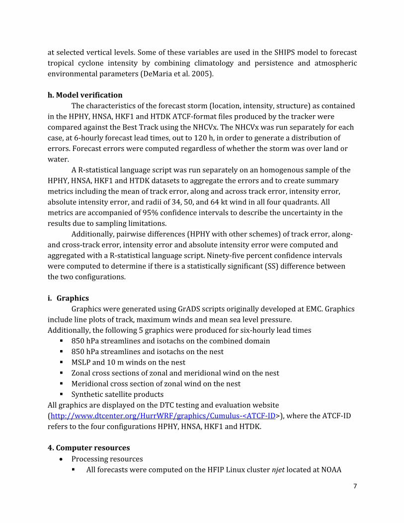
The mean along-track errors (Fig. 4) are near zero for the first two days of forecast.

For longer lead times, they are negative (but not SS) for HPHY, HNSA, and HKF1. Mean

along track errors for HTDK at longer lead times are positive (tracks too fast) and SS

different from the other configurations. The large along track errors for HTDK lead this

configuration to have the larger total track error than the others.

The mean cross track errors (Fig. 5) are near zero for all configurations for the first

two days of forecast. After that, they are negative for HNSA and HKF1, indicating that the

forecast tracks are to the left of the observed ones. The HPHY and HTDK configuration have

the smaller mean cross track errors, and they are only SS different from zero (negative) in

the 3rd day of forecast.

11

Figure 4. Same as Fig. 2, except for along-track mean error (nm).

Figure 5. Same as Fig. 2, except for cross-track mean error (nm).

Figure 6 shows that all configurations have very similar intensity mean absolute

error in the first four days of forecast. Very few SS differences occur between HPHY and the

other configurations as denoted in Table 3. In the last day of forecast, two sets of solution

emerge. HPHY and HNSA, which have similar SAS parameterizations, yield similar errors,

while HKF1 and HTDK have smaller errors. The intensity mean errors (ME), also referred

12

to as biases (Fig. 7), indicate that all schemes start with a small SS negative bias. HPHY has

near-zero bias till 60 h and positive bias thereafter indicating over-intensification. The

other configurations retain a negative bias throughout most of the forecast, but at some

point all configurations transition to positive bias. HKF1 and HTDK have relatively less

positive bias (not SS) after 96 h compared to HNSA and HPHY.

Figure 6. Same as Fig. 2, except for absolute intensity error (kt).

Table 3. Same as Table 2 but for intensity errors (kt).

12 24 36 48 60 72 84 96 108 120

HNSA

HKF1

HTDK

13

Figure 7. Same as Fig. 2, except for intensity mean error (kt).

Fig. 8 shows modified box plots of intensity errors for all the four configurations as a

function of forecast lead times. It is interesting to note that, later in the forecast period,

when all configurations display near-zero or positive bias, the majority of the outliers are

negative.

Figure 8. Same as Fig. 5 but for intensity error (kt).

14

The ME for the wind radii for the 34-, 50-, and 64-kt thresholds for the individual

quadrants is available in Appendix D. To provide overall results on the performance of the

four cumulus schemes, errors averaged over the four quadrants are presented here. A

comparison between the results in the individual quadrants and the averaged values

indicates that the average is a good representation and, with very few exceptions the

individual quadrants do not stand out.

The average ME for the 34-kt wind radius (Fig. 9) indicates that the forecast storms

are large compared to the observed ones. The HNSA makes the storm larger than the other

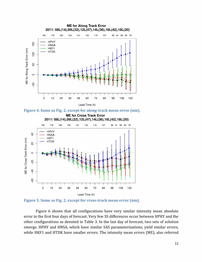
schemes on the 4th and 5th day of forecast. The ME for the 50-kt wind radius (Fig. 10)

indicates that, while all schemes make the storms too large, the configurations that use SAS

(HPHY and HNSA) lead to the larger storms. The separation in two groups (HPHY and

HNSA versus HFK1 and HTDK) is even more robust for 64 kt wind radius (Fig. 11), with

HKF1 and HTDK having less size bias than HPHY and HNSA. This is also reflected in the

intensity ME, which was lower for HKF1 and HTDK. As seen from Bender et al. (1993),

improvement in the storm structure can lead to better intensity forecast. It is also to be

noted that, at the initial time, the forecast storm is already SS too large when compared to

the observed for all wind radii, quadrants and configurations.

Figure 9. Same as Fig. 2, except for 34-kt wind radius mean error (nm) averaged over

the NW, NE, SW and SE quadrants.

15

Figure 10. Same as Fig. 2, except for 50-kt wind radius mean error (nm).

Figure 11. Same as Fig. 2, except for 64-kt wind radius mean error (nm).

Previous studies of the observed maximum wind and minimum pressure (Knaff and

Zehr 2007, Atkinson and Holliday 1997 and several others) have shown that

environmental pressure and storm motion can influence their relationship. Fig. 12 shows a

scatterplot of HPHY MSLP and maximum intensity for both the observed (filled brown

16

circles) and forecast storms at selected lead times (shown in different colors). A subjective

analysis indicates that the forecasts are well aligned with the observations. An objective

analysis is beyond the scope of this report. It is to be kept in mind that all the model

forecasts are shown here, which includes forecasts that are not verified (for example

because the observed storm dissipated). Note that the best track values are only available

in 5-kt increments. Scatterplots for the other configurations are provided in Appendix D.

Figure 12. Scatter plot of intensity (kt) versus MSLP (hPa) for HPHY in the Atlantic

basin. The lead times are shown in different colors and are provided in the rightmost

corner of the plots. The best track values are shown in brown filled circles.

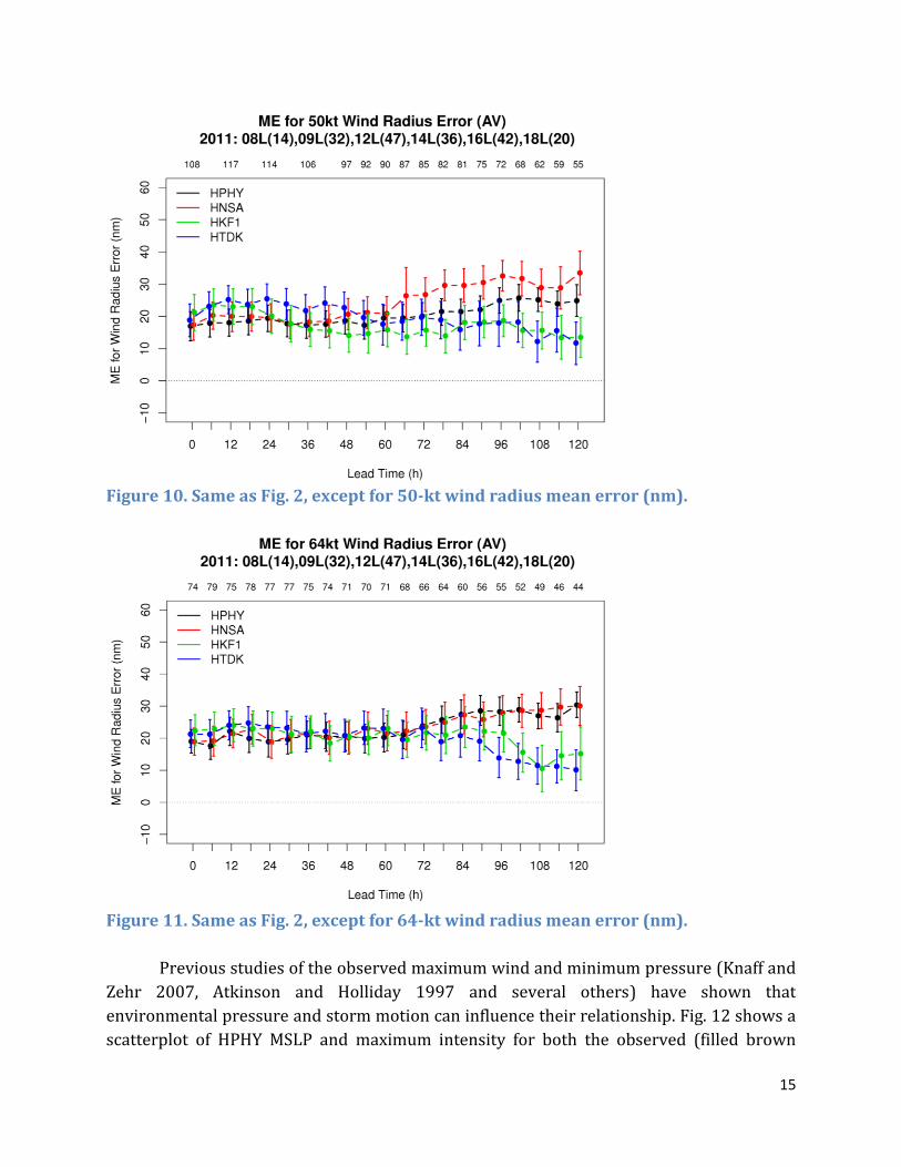
The scatter plots of wind radii errors versus intensity errors (Fig. 13a,b) show that

storms whose size is overestimated are associated with over-estimated intensity. This

patter is most prominent for the 50- and 64-kt radii errors. Due to similar trends in the

results for different schemes, only HPHY is shown here (additional plots are available in

Appendix D).

17

Figure 13a. Scatter plot of intensity error (kt) versus 50-kt wind radius mean error

(nm) averaged over the NW, NE, SW and SE quadrants for HPHY in the Atlantic basin.

The lead times are shown in different colors and are provided in the corner of the

plots.

Figure 13b. Same as Fig 13a, except for 64-kt wind radius

18

There is no clear relationship between track and intensity errors (Fig. 14). So, for

this sample it is not possible to conclude that larger track errors produced large intensity

errors or vice-versa.

Figure 14. Scatterplot of intensity (kt) versus track (nm) errors in the Atlantic basin

for HPHY. The forecast lead times are provided on the right side.

b. Eastern North Pacific

The track MAE (Fig. 15) for the EP is higher than for AL for all configurations, HPHY

has lower mean errors compared to the other schemes but few of the differences are SS –

unlike for AL (Table 4). As described in Appendix A, the number of cases for EP is much

smaller than for AL and hence conclusions after 72 h are questionable. It should be noted

that HTDK does not stand out as the worse configuration as it did for AL.

19

Figure 15. Mean track error (nm) for HPHY (black), HNSA (red), HKF1 (green) and HTDK (purple) as a function of forecast lead time for all cases in the Eastern Pacific basin. The 95% confidence intervals are also displayed. The sample size is listed above the graphic. Table 4. Analysis of statistical significance of the pairwise difference of track errors between HPHY and the other configurations (HNSA, HKF1, and HTDK) for several forecast lead times (h) for EP. A white cell indicates the difference is not SS. A green/red cell indicates the difference is SS and that HPHY has less/more error than the other configuration.

12 24 36 48 60 72 84 96 108 120

HNSA

HKF1

HTDK

Fig 16 shows modified boxplots of track errors along with IQRs and outliers. For EP,

the HNSA and HKF1 configurations have larger outliers at intermediate lead times (48

through 72 h).

20

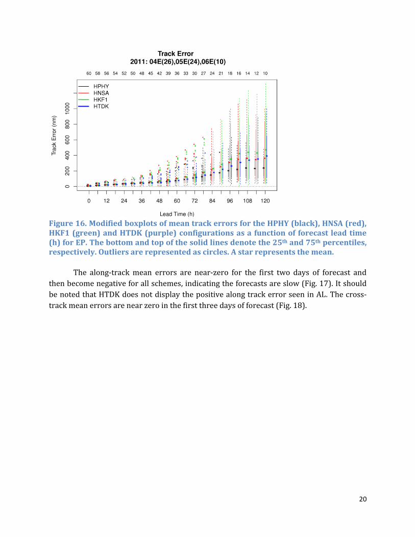
Figure 16. Modified boxplots of mean track errors for the HPHY (black), HNSA (red), HKF1 (green) and HTDK (purple) configurations as a function of forecast lead time (h) for EP. The bottom and top of the solid lines denote the 25th and 75th percentiles, respectively. Outliers are represented as circles. A star represents the mean.

The along-track mean errors are near-zero for the first two days of forecast and

then become negative for all schemes, indicating the forecasts are slow (Fig. 17). It should

be noted that HTDK does not display the positive along track error seen in AL. The cross-

track mean errors are near zero in the first three days of forecast (Fig. 18).

21

Figure 17. Same as Fig. 15, except for along-track mean error (nm).

Figure 18. Same as Fig. 15, except for cross-track mean error (nm).

22

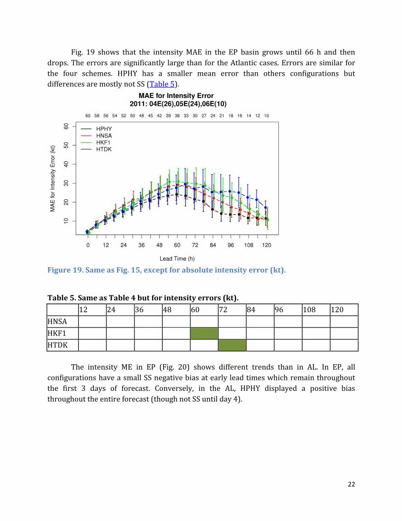
Fig. 19 shows that the intensity MAE in the EP basin grows until 66 h and then

drops. The errors are significantly large than for the Atlantic cases. Errors are similar for

the four schemes. HPHY has a smaller mean error than others configurations but

differences are mostly not SS (Table 5).

Figure 19. Same as Fig. 15, except for absolute intensity error (kt).

Table 5. Same as Table 4 but for intensity errors (kt).

12 24 36 48 60 72 84 96 108 120

HNSA

HKF1

HTDK

The intensity ME in EP (Fig. 20) shows different trends than in AL. In EP, all

configurations have a small SS negative bias at early lead times which remain throughout

the first 3 days of forecast. Conversely, in the AL, HPHY displayed a positive bias

throughout the entire forecast (though not SS until day 4).

23

Figure 20. Same as Fig. 15, except for intensity mean error (kt).

Fig 21 shows modified boxplots for intensity error. It is important to note that even

when the intensity bias is negative, there are many forecasts with positive intensity error.

Figure 21. Same as Figure 16, but for Intensity errors (kt).

24

The ME for 34-, 50- and 64- kt wind radii averaged over the four quadrants provides

the same message as when considered separately. For the 34-kt wind radii (Fig. 22) all the

configurations start with near-zero bias, shift to a small positive bias in the first day of

forecast, and then transition to near-zero (HPHY) or negative bias (other configurations)

for the second and third day of forecast. This result is in sharp contrast with AL, for which

the storm was too large for all configurations at all lead times.

Figs 23 and 24 show the 50- and 64-kt wind radii errors. The initial wind radii

errors increase (become more positive and SS) with the intensity threshold indicating that

all the schemes are having difficulty with initialization. The excessive storm size persists

for the first 24 to 36 h and thereafter the results are not SS.

Figure 22. Same as Fig. 15, except for 34-kt wind radius mean error (nm) averaged

over the NW, NE, SW and SE quadrants.

25

Figure 23. Same as Fig. 15, except for 50-kt wind radius mean error (nm) averaged

over NW, NE, SW and SE quadrants.

Figure 24. Same as Fig. 15, except for 64-kt wind radius mean error (nm) averaged

over NW, NE, SW and SE quadrants.

The wind-pressure plots (Fig. 25) for the four configurations show similar results.

Note that these are all forecasts, not just the ones that were verified. Similar to Atlantic

26

basin, the model forecasts are well aligned with the observations. A striking feature among

all the configurations is presence of forecasts with very low MSLP for a given wind speed,

especially at the initial time (black circles). An example is provided in Figs 26 and 27. This

particular case is from Dora initialized at 2011 July 21 12Z. The model was initialized with

the storm intensity that was provided in the TC Vitals but the initial minimum pressure is

too low (Fig 27). Thus, there are problems with the wind-pressure relationship in the

HWRF model which may be addressed in the vortex relocation procedure.

Figure 25. Scatter plot of intensity (kt) versus MSLP (hPa). The lead times are shown

in different colors and are provided in the top right corner of the plots. The best

track values are shown in brown filled circles.

27

Figure 26. Intensity forecast for Dora for HPHY initialized 12Z July 21 2011. The

black line with hurricane symbols is the best track, and forecasts are shown for the

HPHY (black), HNSA (red), HKF1 (green) and HTDK (blue) configurations.

Figure 27. Same as Fig. 26 but for MSLP (hPa).

The scatter plots of intensity errors versus wind structure errors for all

configurations (Fig. 28 and Appendix D) indicate that the storm tends to be too strong and

too big or too weak and too small. This was also seen by Liu and Pan of EMC (August 2012

HFIP Workshop).

28

Figure 28. Scatter plot of intensity error (kt) versus 34-kt wind radius mean error

(nm) averaged over the NW, NE, SW and SE quadrants for HPHY in EP. The lead times

are shown in different colors and are provided in the top right corner of the plot.

7. Interpretation and conclusions

This is the first extensive test conducted by DTC in 2012. Its goal was to document

the HWRF sensitivity to different cumulus parameterizations.

It is to be noted that the 2012 operational HWRF implementation differs from HPHY

(developmental code as of February 2012) in a few important aspects. The 2012

operational configuration employs a shallow convection scheme, uses assimilation of

conventional data in the storm environment (1,200 km or more away from the storm

center), uses 45/15/5 s dynamic time steps and 180/180/180 s physics time steps for

domain 1, 2, and 3, respectively. While these modifications impact the forecast (Fovell,

2012, HFIP Teleconference presentations), they are not expected to invalidate the

conclusions.

No configuration outperformed HPHY so no recommendation was made to change

the operational HWRF configuration. The HWRF SAS produced superior tracks for the

Atlantic and most of the other measures showed little SS differences between the various

configurations.

While HPHY shows intensity over-prediction in the AL, which is somewhat

mitigated when other schemes were employed, the intensity MAE were not reduced when

using alternate configurations. In fact, intensity MAEs were larger in the EP for the

alternate configurations (though not SS).

29

The analysis of structure versus intensity errors indicates that HWRF tends to make

the storms too large and intense or weak and small. This phenomenon has also seen by Liu

and Pan (2012, presentation at the Physics Workshop of the HFIP Regional Modeling

Team), who have shown that utilizing the new meso-SAS cumulus parameterization

scheme in the 3-km grid can improve the structure and intensity forecasts by reducing the

resolved convection.

9. References

Atkinson, G. D., and C. R. Holliday, 1977: Tropical cyclone minimum sea level

pressure/maximum sustained wind relationship for the western North Pacific. Mon. Wea.

Rev., 105, 421–427.

Bao et al. 2012: HWRF Community HWRF Users’ Guide V 3.4a, 2012:

(http://www.dtcenter.org/ HurrWRF/users/docs/users_guide/HWRF_UG_v3.4a.pdf)

Bender, Morris A., Rebecca J. Ross, Robert E. Tuleya, Yoshio Kurihara, 1993: Improvements

in Tropical Cyclone Track and Intensity Forecasts Using the GFDL Initialization System.

Mon. Wea. Rev., 121, 2046–2061.

DeMaria, M., M. Mainelli, L. K. Shay, J. A. Knaff, and J. Kaplan, 2005: Further Improvements

to the Statistical Hurricane Intensity Prediction Scheme (SHIPS). Wea. Forecasting, 20,

531.543.

Gopalakrishnan et al. 2012: Hurricane Weather Research and Forecasting (HWRF) Model:

2012 Scientific Documentation, 2012: (http://www.dtcenter.org/HurrWRF/users/docs/

scientific_documents/HWRFScientificDocumentation_v3.4a.pdf)

Knaff, John A., Raymond M. Zehr, 2007: Reexamination of Tropical Cyclone Wind–Pressure

Relationships. Wea. Forecasting, 22, 71–88.

Acknowledgements

The DTC is funded by NOAA, the Air Force Weather Agency, and NCAR. This work was

partially supported by NOAA HFIP.

30

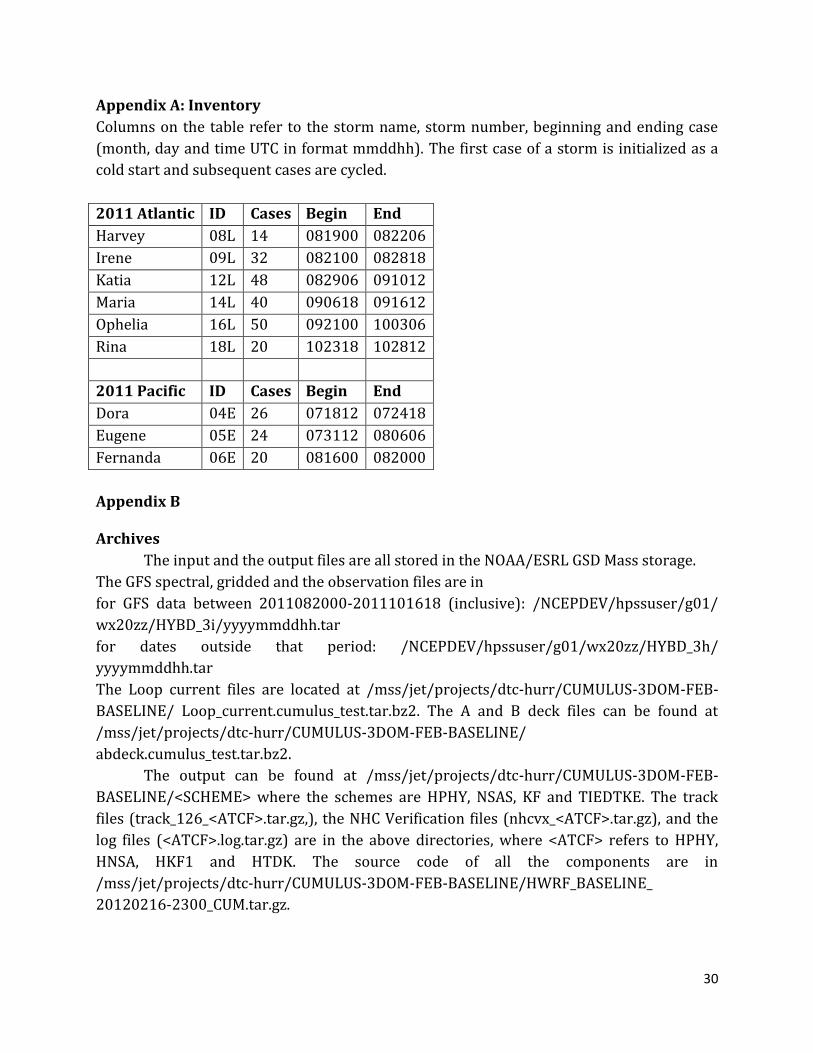
Appendix A: Inventory

Columns on the table refer to the storm name, storm number, beginning and ending case

(month, day and time UTC in format mmddhh). The first case of a storm is initialized as a

cold start and subsequent cases are cycled.

2011 Atlantic ID Cases Begin End

Harvey 08L 14 081900 082206

Irene 09L 32 082100 082818

Katia 12L 48 082906 091012

Maria 14L 40 090618 091612

Ophelia 16L 50 092100 100306

Rina 18L 20 102318 102812

2011 Pacific ID Cases Begin End

Dora 04E 26 071812 072418

Eugene 05E 24 073112 080606

Fernanda 06E 20 081600 082000

Appendix B Archives

The input and the output files are all stored in the NOAA/ESRL GSD Mass storage.

The GFS spectral, gridded and the observation files are in

for GFS data between 2011082000-2011101618 (inclusive): /NCEPDEV/hpssuser/g01/

wx20zz/HYBD_3i/yyyymmddhh.tar

for dates outside that period: /NCEPDEV/hpssuser/g01/wx20zz/HYBD_3h/

yyyymmddhh.tar

The Loop current files are located at /mss/jet/projects/dtc-hurr/CUMULUS-3DOM-FEB-

BASELINE/ Loop_current.cumulus_test.tar.bz2. The A and B deck files can be found at

/mss/jet/projects/dtc-hurr/CUMULUS-3DOM-FEB-BASELINE/

abdeck.cumulus_test.tar.bz2.

The output can be found at /mss/jet/projects/dtc-hurr/CUMULUS-3DOM-FEB-

BASELINE/<SCHEME> where the schemes are HPHY, NSAS, KF and TIEDTKE. The track

files (track_126_<ATCF>.tar.gz,), the NHC Verification files (nhcvx_<ATCF>.tar.gz), and the

log files (<ATCF>.log.tar.gz) are in the above directories, where <ATCF> refers to HPHY,

HNSA, HKF1 and HTDK. The source code of all the components are in

/mss/jet/projects/dtc-hurr/CUMULUS-3DOM-FEB-BASELINE/HWRF_BASELINE_

20120216-2300_CUM.tar.gz.

31

Files archived in the MSS

Messages o domain_center o tcvital

geogrid output o geo_nmm* o namelist.wps

real output o namelist.input o fort.65 o wrfinput_d01

WRF ghost output o ghost_d02_0000-00-00_00:00:00 o ghost_d03_0000-00‐00_00:00:00

WRF analysis output o wrfanl_d02_yyyy-mm-dd_hh:00:00 o wrfanl_d03_yyyy-mm-dd_hh:00:00

Vortex relocation output o wrfinput_d01 o wrfinput_d02 o wrfinput_d03 o wrfghost_d02

Ocean Initialization output o ocean_region_info.txt o getsst/mask.gfs.dat o getsst/sst.gfs.dat o getsst/lonlat.gfs o phase4/track o logs o getsst/getsst.out o phase3/phase3.out o phase4/phase4.out o sharpn/sharpn.out

Coupled WRF-POM run input and output o RST.final o wrfinput_d01 o wrfbdy_d01 o wrfanl_d02_yyyy-mm-dd_hh:00:00 o wrfanl_d03_yyyy-mm-dd_hh:00:00 o EL.* o GRADS.* o OHC.* o T.* o TXY.* o U.* o V.* o WTSW.* o rsl.*

Postprocessing output o WRFPRS*

Tracker output o Combined domain

o Long track (126h forecast) from forecasts at 6-h intervals

32

o Short track (12h forecast) from forecasts at 3-h intervals o 12-h 3-hrly fort.64 o 126-h 6-hrly fort.64

o Parent domain o Long track (126h forecast) from forecasts at 3-h intervals o 126-h 3 -hrlyfort.64

Graphics output o hwrf_plots/${SID}.${yyyymmddhh}/*gif

SHIPS Diagnostic Output

o sal*

Appendix C: List of acronyms AL – North Atlantic basin ATCF – Automated Tropical Cyclone Forecasting BC – Boundary Conditions DTC – Developmental Testbed Center EMC – Environmental Modeling Center EP – Eastern North Pacific basin GFDL – Geophysical Fluid Dynamics Laboratory GFS – Global Forecasting System GSD – Global Systems Division (of NOAA Earth System Research Laboratory) GSI – Global Statistical Interpolator GRIB – Gridded binary data format HFIP – Hurricane Forecast Improvement Project HKF1 – HWRF configuration using the Kain Fritsch cumulus scheme HNSA – HWRF configuration using the New SAS cumulus scheme implemented by YSU HPHY – HWRF configuration using theSAS cumulus scheme as of February 2012 HTDK – HWRF configuration using the using the Tiedtke cumulus scheme HWRF – Hurricane Weather Research and Forecasting IC – Initial Conditions IQR – Inter-quartile range MAE – mean absolute error MSLP – Mean Sea Level Pressure MSS – Mass Storage System NCEP – National Centers for Environmental Prediction NHC – National Hurricane Center NHCVx --‐ National Hurricane Center verification package NMM – Non--‐hydrostatic Mesoscale Model NOAA – National Oceanic and Atmospheric Administration NSAS – SAS scheme implemented by Yonsei University POM – Princeton Ocean Model Pre13hi GFS – Retrospective runs made with GFS SAS – Simplified Arakawa Schubert cumulus parameterization SID – Storm Identification SHIPS – Statistical Hurricane Intensity Prediction Scheme SS – Statistically significant UPP – Unified Post-Processor WPS – WRF Preprocessing System WRF – Weather Research and Forecasting

T&E – Testing and Evaluation

YSU – Yonsei University of South Korea

SW- Short Wave

33

LW- Long Wave

CIRA- Collaborative Institute for Research in the Atmosphere