The Development of the UNIFAC-CONDUCT Model as a NovelApproach for the Estimation of the Conductivity of Pure Ionic Liquids

Zhao, N., & Jacquemin, J. (2017). The Development of the UNIFAC-CONDUCT Model as a Novel Approach forthe Estimation of the Conductivity of Pure Ionic Liquids. Fluid Phase Equilibria.https://doi.org/10.1016/j.fluid.2017.06.010

Published in:Fluid Phase Equilibria

Document Version:Peer reviewed version

Queen's University Belfast - Research Portal:Link to publication record in Queen's University Belfast Research Portal

Publisher rightsCopyright 2017 Elsevier.This manuscript is distributed under a Creative Commons Attribution-NonCommercial-NoDerivs License(https://creativecommons.org/licenses/by-nc-nd/4.0/), which permits distribution and reproduction for non-commercial purposes, provided theauthor and source are cited.

General rightsCopyright for the publications made accessible via the Queen's University Belfast Research Portal is retained by the author(s) and / or othercopyright owners and it is a condition of accessing these publications that users recognise and abide by the legal requirements associatedwith these rights.

Take down policyThe Research Portal is Queen's institutional repository that provides access to Queen's research output. Every effort has been made toensure that content in the Research Portal does not infringe any person's rights, or applicable UK laws. If you discover content in theResearch Portal that you believe breaches copyright or violates any law, please contact openaccess@qub.ac.uk.

Download date:27. Feb. 2020

The Development of the UNIFAC-CONDUCT Model as a Novel Approach

for the Estimation of the Conductivity of Pure Ionic Liquids

Nan Zhao1, Johan Jacquemin1,2,*

1 School of Chemistry and Chemical Engineering, Queen’s University Belfast, Belfast,

BT9 5AG, U.K.

2 Universite Francois Rabelais, Laboratoire PCM2E, Parc de Grandmont 37200 Tours,

France

Corresponding Author: Johan Jacquemin, E-mail: johan.jacquemin@qub.ac.uk or

jj@univ-tours.fr

Abstract

The correlation and prediction of physical properties of ionic liquids (ILs) is important

in the development and design of novel structures for a variety of applications. In

particular, for the application as electrolytic media for electrochemical applications,

the electrical conductivity of ILs is an important property. Herein, we define a novel

model called the UNIFAC-CONDUCT for the estimation of IL conductivity which

mimics the principles of the UNIFAC-VISCO model. 784 data points for 38 ILs were

used to establish this group contribution model, covering a wide range of

temperature (248.15-468.15 K) and a broad range of electrical conductivity

(0.002-14.54 S·m-1). Three sets of UNIFAC-CONDUCT parameters were determined to

calculate the conductivity of pure ILs by three methodologies wherein the

parameters of ion VFT equations, A, B and To, and binary interaction parameters, αmn,

are selectively either fixed (based on previously reported values) and/or optimized

by Marquardt technique. Correlations by the three methods are compared and

analyzed, and further correlated with the previously predicted viscosities using the

Nernst-Stokes relationship to support the quality of both the UNIFAC-VISCO model,

previously proposed by our group, and the UNIFAC-CONDUCT model developed in

this paper. Finally, the quality of the proposed method was further assessed through

the prediction of the conductivity of one binary system containing two different ILs

as the function of the temperature and composition with an accuracy close to 4.1 %.

Keywords: Ionic Liquids; Conductivity; Temperature; UNIFAC-CONDUCT; Group

Contribution Model

1. Introduction

Ionic liquids (ILs) are organic salts that are liquid at temperature below 100 °C [1].

Recently, ILs have been investigated increasingly in industry and academia, due to

their low vapor pressure, high conductivity, wide electrochemical window, and

chemical and thermal stability. It is well-recognized that one of the most promising

application for ILs is their use as electrolytes for energy storage systems, such as

batteries, fuel cells and supercapacitors [2]. For these applications, the design of

task-specific ILs with high ionic conductivity is crucial. Hence, a thorough knowledge

of their conductivities is essential to formulate novel electrolytes [3]. Taking into

account the number of possible IL combinations, the development of methods able

to estimate accurately their properties is highly desired.

Literature models have been reported for the prediction and correlation of ionic

conductivity of pure ILs. The first approach is to relate the conductivity to other

properties of ILs. Slattery et al. [4] reported a strong relationship between the

molecular volumes, 𝑉𝑚, and conductivities, σ, of ILs, as shown in eq. 1.

𝑙𝑛𝜎 = −𝑑𝑉𝑚 + 𝑙𝑛ℎ (1)

where 𝑑 and ℎ are fitting parameters.

Using this relationship, these authors correlated the experimental conductivities of

[NTf2]-, [DCA]-, [BF4]-, and [PF6]- based ILs using eq. 1 with 𝑅2 being 0.9871 [4].

However, in this instance, limited data points were used; only 12, 3, 3, and 3 data

points for [NTf2]-, [DCA]-, [BF4]-, and [PF6]- based ILs, respectively.

In addition, Bogdanov et al. [5] proposed another linear correlation (eq. 2) between

the conductivity of 𝑋 -substituted ILs and substituent constant, 𝛽𝑋 , for each

homologous series of ILs. In total 69 experimental data points, covering 17

homologous series of ILs, were selected, with the fitting result (𝑅2) better than

0.9615.

𝑙𝑛𝜎 = 𝑎𝛽𝑋 + 𝑙𝑛𝜎0 (2)

where, a and 𝜎0 are a fitting parameter and the conductivity of the

methyl-substituted IL of a homologous series, respectively.

The second approach is the group contribution model for the prediction of the

electrical conductivity of ILs. Gardas and Coutinho [6] calculated the adjustable

parameters (𝐴 and 𝐵) of the Vogel-Fulcher-Tammann (VFT) equation (eq. 3) by

using a group contribution method (eqs. 4-5) by fixing the fitting parameter related

to the temperature, 𝑇0, to 165.06 K for all ILs studied.

𝑙𝑛𝜎 = 𝑙𝑛𝐴 +𝐵

𝑇−𝑇0 (3)

𝐴 = ∑ 𝑛𝑖𝑎𝑖𝑁𝑖=1 (4)

𝐵 = ∑ 𝑛𝑖𝑏𝑖𝑁𝑖=1 (5)

where 𝑁 is the total number of different groups in the IL, 𝑛𝑖 is the number of

occurrences of group 𝑖, and 𝑎𝑖 and 𝑏𝑖 are parameters of group 𝑖. In total 307

experimental data points from 15 ILs were regressed to obtain the group parameters

𝑎𝑖 and 𝑏𝑖, with a 4.57% overall relative deviation between the experimental data

and the correlated values.

Similar to the method proposed by Gardas and Coutinho [6], and Wu et al. [3]

expressed the adjustable parameters (𝐴, 𝐵, and 𝑇0) of the VFT equation using a

series of more complicated group contribution equations (eqs. 6-8).

𝐴 = 𝐴0 + ∑ ∑ 𝑛𝑖𝑚(𝑊𝐴𝑚,𝑖)

𝑁𝑖=1

2𝑚=1 (6)

𝐵 = (𝐵0 + ∑ ∑ 𝑛𝑖𝑚(𝑊𝐵𝑚,𝑖)(𝐵0

′ + ∑ ∑ 𝑛𝑖𝑚(𝑊𝐵𝑚,𝑖

′ )𝑁𝑖=1 )2

𝑚=1𝑁𝑖=1

2𝑚=1 (7)

𝑇0 = 𝑇0′ + ∑ ∑ 𝑛𝑖

𝑚(𝑊𝑇0𝑚,𝑖)𝑁𝑖=1

2𝑚=1 (8)

where 𝑊𝐴𝑚,𝑖 , 𝑊𝑇0𝑚,𝑖 , 𝑊𝐵𝑚,𝑖 and 𝑊𝐵𝑚,𝑖′ are contributions of the 𝑚 th-order

group 𝑖, 𝐴0, 𝑇0, 𝐵0, and 𝐵0′ are values of all computed coefficients. Herein, the

observed deviations between the experimental and evaluated results for training

(1978 data points of 177 ILs) and testing (217 data points of 11 ILs) were 6.12% and

5.10%, respectively.

Gharagheizi et al. [7] proposed a least square support vector machine-group

contribution (LSSVM-GC) model for the estimation of pure conductivity. Parameters

𝜎𝑐𝑖 (𝑖=1, 2, … 11) of 11 sub-structures on cations and parameters 𝜎𝑎𝑖 (𝑖=1, 2, … 11)

of 11 sub-structures on anions were used to establish this group contribution model.

An average deviation of 3.3% is acceptable given that 1077 experimental

conductivities for 54 ILs were predicted. However, the complexity of this model limits

its applicability to a wider range of types of ILs.

The fourth approach reported in the literature is based on the hole theory. Abbott [8]

first applied the hole theory to predict the viscosity of ILs. Afterwards, Zhao et al. [9]

modified the hole theory model to facilitate the estimation of the conductivity of ILs

and reported a comparison of the new and conventional hole models by utilizing a

range of 24 ILs (one data point for each IL). They report that the estimation accuracy

of the new methodology was increased from the order of 27%, by the original

method, to 11.87%.

Tochigi et al. [10,11] proposed two different Quantitative Structure Property

Relationship methods (QSPR) for the estimation of conductivity of ILs. Two different

sets of descriptors, establishing two different polynomial expansion models, were

used to calculate the conductivity of ILs. However, it is not convenient to apply these

methods due to the complexity of the polynomial expansions.

In this work, we define a novel model called the UNIFAC-CODUCT, on the basis of the

UNIFAC model, for the estimation of the conductivity of pure ILs. 784 experimental

conductivities of 38 ILs were collected from the NIST database [12], covering a wide

range of temperature (248.15 – 468.15 K) and electrical conductivity (0.002 – 14.54

S·m-1) to establish the UNIFAC-CONDUCT model as reported in Table 1 [13-39].

According to the NIST database, the uncertainty of the conductivity datasets

reported in the literature is within ± 3 % [12].

2. Methodology

2.1 The UNIFAC-CONDUCT model.

In our previous paper [40,41], new methods based on the UNIFAC-VISCO model have

been reported for the evaluation of the viscosity of pure ILs, and their mixtures with

another IL or molecular solvent, (IL + IL) or (IL + solvent) binary mixtures as the

function of temperature and composition at atmospheric pressure. It is very

well-known that the conductivity is a nonlinear property and, like viscosity, can be

fitted by using the simple exponential equations, such as Arrhenius, Litovitz, and VFT

equations [42]. Consequently, the UNIFAC-based model, namely the

UNIFAC-CONDUCT, was developed herein to estimate the conductivity of pure ILs.

The equations of the UNIFAC-CONDUCT model, described below, are similar to the

UNIFAC-VISCO formulations described by our group previously [40].

The conductivity in the UNIFAC-CONDUCT method is defined as:

𝑙𝑛𝜎 = ∑ 𝑥𝑖 ln (𝜎𝑖 ∙𝑉𝑖

𝑉𝑚) +

𝑔𝑐𝐸

𝑅𝑇−

𝑔𝑟𝐸

𝑅𝑇

𝐶𝑖=1 (9)

Herein, subscript 𝑖 represents the component 𝑖 in the pure IL (i.e., the cation and

anion); 𝐶 is the number of the components in the IL and equal to 2; 𝑥𝑖 is the mole

fraction of the cation/anion (𝑥1 = 𝑥2 = 0.5); 𝜎𝑖 is the conductivity of the ion and

expressed by using the VFT equation (eq. 10); 𝑉𝑖 is the effective molar volume of

the ion and calculated based on a group contribution method previously proposed by

our group [43,44]; 𝑉𝑚 is the molar volume of the pure IL;

𝜎𝑖 = 𝐴 ∙ exp[−𝐵

𝑇−𝑇0] (10)

𝑉𝑖(𝛿𝑇, 𝑝𝑟𝑒𝑓) = ∑ (𝐷𝑖 ∙ (𝛿𝑇)𝑝𝑟𝑒𝑓𝑖 )2

𝑖=0 (11)

where 𝛿𝑇 = 𝑇 − 298.15, 𝑝𝑟𝑒𝑓 = 0.1 MPa, and 𝐷𝑖 is the volumetric parameters at

reference pressure. The values of the volumetric parameters used during this work

are presented in Table S1 of the Supporting Information.

The UNIFAC-CONDUCT combinatorial term reported in the eq. 9 is defined by:

𝑔𝑐𝐸

𝑅𝑇= ∑ 𝑥𝑖𝑙𝑛

𝜙𝑖

𝑥𝑖+ 5∑ 𝑥𝑖𝑞𝑖𝑙𝑛

𝜃𝑖

𝜙𝑖

𝐶𝑖=1

𝐶𝑖=1 (12)

where

𝜃𝑖 =𝑥𝑖𝑞𝑖

∑ 𝑥𝑗𝑞𝑗𝑗 (13)

𝜙𝑖 =𝑥𝑖𝑟𝑖

∑ 𝑥𝑗𝑟𝑗𝑗 (14)

𝑞𝑖 = ∑ 𝑛𝑖,𝑘𝑄𝑘𝑁𝑘=1 (15)

𝑟𝑖 = ∑ 𝑛𝑖,𝑘𝑅𝑘𝑁𝑘=1 (16)

where subscript 𝑘 denotes the groups; 𝑁 is the total number of groups present;

𝑛𝑖,𝑘 is the total number of 𝑘𝑡ℎ group present in component 𝑖; 𝑄𝑘 and 𝑅𝑘 are the

group surface area parameter and volume parameter, respectively. The values of

volume 𝑅 and surface area 𝑄 parameters of ions used were simulated by using the

COSMOtherm software (version C30_1501) by following the methodology previously

described by our group [45], and are given in the Table S2 of the Supporting

Information.

The UNIFAC-CONDUCT residual term reported in the eq. 9 is defined by:

𝑔𝑟𝐸

𝑅𝑇= ∑ 𝑥𝑖[∑ 𝑛𝑚,𝑖(𝑙𝑛𝛾𝑚 − 𝑙𝑛𝛾𝑚,𝑖)

𝑁𝑚=1 ]𝐶

𝑖=1 (17)

where 𝑙𝑛𝛾𝑚 is the residual activity coefficient and can be calculated as follows:

𝑙𝑛𝛾𝑚 = 𝑄𝑚[1 − ln(∑ Θ𝑖Ψ𝑖,𝑚𝑁𝑖=1 ) − ∑

Θ𝑖Ψ𝑚,𝑖

∑ Θ𝑗Ψ𝑗,𝑖𝑁𝑗=1

𝑁𝑖=1 ] (18)

where

Θ𝑚 =𝑋𝑚𝑄𝑚

∑ 𝑋𝑖𝑄𝑖𝑁𝑖=1

, 𝑚 = 1, 2, 3, …, N (19)

Ψ𝑚𝑛 = exp(−𝛼𝑚𝑛

298.15) (20)

where 𝛼𝑚𝑛 are the group interaction potential energy parameters between 𝑚 and

𝑛, determined through the regression of the collected experimental data as reported

in the Supporting Information. Herein, the COSMOthermX software was used to

determine only the group surface area (𝑄𝑘) and volume (𝑅𝑘) parameters,

which are required for the calculation of the UNIFAC-CONDUCT combinatorial

term.

In our previous work, a set of binary interaction parameters 𝛼𝑚𝑛 between ionic

groups and a set of VFT parameters (𝐴, 𝐵, and 𝑇0) for the effective viscosity of ions

have been reported [41]. Herein, three methods were applied for the estimation of

pure ILs conductivity and the results determined by these three methods are

compared and analyzed. To obtain the unknown parameters, we performed the

Marquardt optimization [46] of the objective function (OF), as reported in eq. 21.

𝑂𝐹 =1

𝑀∑ (

𝜎𝑒𝑥𝑝−𝜎𝑐𝑎𝑙

𝜎𝑒𝑥𝑝)2𝑀

𝑖=1 → 𝑚𝑖𝑛 (21)

Herein, 784 experimental conductivity data of 38 ILs were regressed altogether and

this regression process was achieved by using a nonlinear least-squares function in

MATLAB Optimization Toolbox. An overview of the experimental data collected for 38

ILs is presented in Table 1. The developed MATLAB program, available in the

supporting information, contains all parameters (binary interaction and VFT

parameters) estimated during this study for each method reported below.

2.2 Method 1: Estimation of IL conductivity by using a fixed set of 𝜶𝒎𝒏 and 𝑻𝟎.

The first method is to fix the values of interaction parameters 𝛼𝑚𝑛 and the values of

reference temperature 𝑇0 for each ion as those described in our previous work for

the UNIFAC-VISCO model [41]. In this case, the unknown parameters are only 𝐴 and

𝐵 of the VFT equations, used to describe the effective conductivity of ions as a

function of temperature.

2.3 Method 2: Estimation of IL conductivity by using a fixed set of 𝜶𝒎𝒏.

For the second method, we only keep the values of 𝛼𝑚𝑛 as reported in our previous

work [41], and the ion VFT parameters (𝐴 , 𝐵 , and 𝑇0 ) were calculated by

minimization of the objective function using all the experimental data.

2.4 Method 3: Estimation of IL conductivity by using a new set of 𝜶𝒎𝒏 and 𝑻𝟎.

The third method is to obtain a totally new set of parameters (𝛼𝑚𝑛 and 𝑇0) which

could be potentially used only for the UNIFAC-CONDUCT model by minimization of

the objective function using all the experimental data.

3. Results and Discussion

Three sets of UNIFAC-CONDUCT parameters (i.e. VFT parameters and binary

interaction parameters 𝛼𝑚𝑛) are listed in Tables S3-S7 of the Supporting Information.

The regression results were demonstrated by calculating the relative absolute

average deviation (RAAD, eq. 22) between the experimental conductivities and the

correlated values.

𝑅𝐴𝐴𝐷 = 100 ×1

𝑀∑ |

𝜎𝑒𝑥𝑝−𝜎𝑐𝑎𝑙

𝜎𝑒𝑥𝑝|𝑀

𝑖=0 (22)

The overall RAAD resulting from the first, second, and the third method is close to

9.9%, 9.2%, and 2.3%, respectively. The parity plots between the experimental and

the calculated values by using these three different methods are shown in Figure 1.

Comparing both plots (a) and (b) reported in Figure 1 and data reported in the

database spreadsheet available in the Supporting Information, it can be noticed that

the values of the parameter 𝑇0 in the VFT equations of ions have a small influence

on the performance of the evaluation of the pure ILs conductivity. However, the

comparison of both plots (b) and (c) from Figure 1 clearly shows that the global

optimized values of 𝛼𝑚𝑛 can significantly increase the accuracy of the

UNIFAC-CONDUCT model during the estimation of the pure ILs conductivity. This is

further exemplified in Figures 2-4 where the effect of temperature, cations and

anions structure on the quality of each correlation is reported. As illustrated in Figure

2 in the case of the [C4mpyrro][NTf2] using the dataset published by Vranes et al. [34],

each method is able to correlate the temperature dependence on the IL conductivity.

Similarly, as shown in Figures 3 and 4, effects of both anion and cation structure on

the conductivity seem to be properly described by each method. From Figure 4, one

can clearly see, as expected from literature data [16,29,30,33,34,36], an increase of

the alkyl chain length from n = 1 to 2 for the series [Cnmim][NTf2] results in a slight

increase in conductivity prior to a marked decrease (for n > 2), for example. However,

it can be also notified from Figure 4 that at 298.15 K, by using both methods 1 and 2

the conductivity data are over or under predicted for short (n < 4) or for long (n > 4)

alkyl chain length, which is not observed in the case of the method 3 as expected.

However, the original idea to keep the values of the 𝑇0 and 𝛼𝑚𝑛 parameters in the

UNIFAC-CONDUCT model similar to those determined for the UNIFAC-VISCO model

[41] has a physical meaning, which may reflect the ILs cohesive energy. Furthermore,

this logic also limits the number of unknown parameters during the regression and

thus the estimation of the conductivity and/or viscosity of pure ILs.

To further assess this approach, viscosity and conductivity data for the [C6mim][eFAP]

and [C4mpyrro][NTf2] were evaluated by using the UNIFAC-VISCO and

UNIFAC-CONDUCT models prior to verifying their relationship in terms of the

Nernst-Einstein and Stokes-Einstein equations. These two ILs have been selected to

represent more hydrolytically and electrochemically stable ILs compared to the

conventional [BF4]- and [PF6]- ILs typically used which are hydrolytically unstable

[1,36]. In particular, the [C4mpyrro][NTf2] is commonly used by several research

groups to formulate electrolytes for energy storage systems [2].

According to the Nernst-Einstein equation, the molar conductivity (Λ ) of an

electrolyte species is related to its self-diffusion coefficient (𝐷) as follows:

Λ =𝑧2𝑁𝐴𝑒0

2𝐷

𝑘𝐵𝑇 (23)

where 𝑧 is the valence of the charge carrier, 𝑁𝐴 is the Avogadro number, 𝑒0 is the

elementary charge, and 𝑘𝐵 is the Boltzmann constant. The molar conductivity (Λ) is

defined as the conductivity (𝜎) divided by the concentration of the charge carriers

(𝑐):

Λ =𝜎

𝑐=

𝜎

𝑛 𝑉⁄=

𝜎

(𝑁 𝑁𝐴⁄ )𝑉⁄

(24)

where, 𝑛 is the moles of the charge carriers, 𝑁𝐴 is the Avogadro number, and 𝑁 is

the number of charge carriers in the volume 𝑉.

Furthermore, the self-diffusion coefficient 𝐷 is defined by the Stokes-Einstein

equation as follows:

𝐷 =𝑘𝐵𝑇

6𝜋𝑟𝜂 (25)

where, 𝑟 is the effective radius and 𝜂 is the viscosity of the charge carriers.

Consequently, the relationship between the conductivity (𝜎) and viscosity (𝜂) is

derived by combining the Eqs. 23-25:

𝜎 =𝑧2𝑒0

2𝑁

6𝑉𝜋𝑟𝜂= 𝑘 ∙

1

𝜂 (26)

where, 𝑘 is the slope.

According to eq. 26, it can be observed that the conductivity is inversely proportional

to the viscosity. Figure 5 shows the calculated conductivity of the selected ionic

liquids by the UNIFAC-CONDUCT model as a function of the inverse viscosity

calculated by the UNIFAC-VISCO model [41], using identical values of a set of

parameters 𝛼𝑚𝑛 and 𝑇0 (first method). As shown in Figure 5, an excellent linear

fitting between the inverse calculated viscosity and the calculated conductivity is

observed, which also proves the evaluation capability of the UNIFAC-VISCO model

previously developed by our group [40,41] and the UNIFAC-CONDUCT model

proposed during this work.

To further assess this approach, the conductivity of the ([C2mim][DCA] +

[C2mim][SCN]) binary system was purely predicted using the UNIFAC-CONDUCT

model with the 𝛼𝑚𝑛 parameters, reported previously, from the UNIFAC-VISCO

model [41]. The literature experimental dataset used during this assessment is also

reported in Table 2 [47]. As shown in Figure 6, an excellent agreement was observed

between the experimental and the predicted conductivity data of the ([C2mim][DCA]

+ [C2mim][SCN]) binary system with an overall relative absolute average deviation

close to 4.1 %. This result is very promising considering, firstly, the approach used, i.e.

using reported parameters for the UNIFAC-VISCO, and secondly, the possibility to

determine the conductivity of this mixture as a function of both composition and

temperature.

4. Conclusion

During this work, a novel model called the UNIFAC-CONDUCT, which mimics the

UNIFAC-VISCO model, is defined for the estimation of the electrical conductivity of

pure ILs. Three different approaches were used to determine unknown

UNIFAC-CONDUCT parameters using the Marquardt optimization technique. All of

them were then assessed using 784 conductivity data points for 38 different ILs as a

function of temperature at atmospheric pressure. As expected, the method 3, which

is based on the optimization of all fitting parameters, provides the best accuracy.

However, by keeping the values of 𝑇0 and 𝛼𝑚𝑛 as those reported in our previous

paper [41], one can appreciate their physical meanings and this approach indeed

reduces the number of unknown parameters for the property estimation by

developing a single set of parameters for these two UNIFAC-based methods. In

addition, the derivation of the formulation between the conductivity and viscosity of

ILs was presented, through the combination of the Nernst-Einstein and

Stokes-Einstein equations. An excellent linear relationship between the calculated

conductivity and the inverse calculated viscosity, also demonstrates the quality of

both the UNIFAC-CONDUCT model proposed herein, and the UNIFAC-VISCO model

previously developed by our group [40,41], as well as the possibility to develop an

unique set of parameters for these two related UNIFAC-based models. In addition,

the conductivity of the ([C2mim][DCA] + [C2mim][SCN]) binary system was purely

predicted using this approach with high accuracy. This demonstrates that the

UNIFAC-CONDUCT model is able to predict the conductivity of binary systems

containing ILs. The prediction of the conductivity of electrolytes (i.e. mixtures of ILs

and/or molten salts and/or molecular solvents) based on the UNIFAC-CONDUCT

model is currently being investigated by our group and will be presented in the near

future.

Supporting Information

An overview of the parameters used to establish the UNIFAC-CONDUCT model in this

work is presented in the Supporting Information in Table S1-S7. Effective molar

volume parameters, 𝑅 and 𝑄 values for each ion are tabulated in Tables S1 and S2,

respectively, while the values of three different sets of UNIFAC-CONDUCT parameters

were listed in Tables S3-S7. Furthermore, the Matlab files used for the calculation of

the conductivity of pure ILs and two separated spreadsheets (named “conductivity

database for pure ILs” and “calculation example”) reporting the database used and

an example of the calculation procedure using the UNIFAC-CONDUCT model are also

provided in the Supporting Information.

Corresponding Author

Johan Jacquemin, E-mail: johan.jacquemin@qub.ac.uk or jj@univ-tours.fr

Acknowledgement

N.Z. and J.J. acknowledge gratefully the CEA le Ripault (Grant No 4600261677/P6E31)

and the Engineering and Physical Sciences Research Council (EPSRC) for supporting

this work financially (EPSRC First Grant Scheme, Grant No EP/M021785/1).

ABBREVIATIONS

Cations:

[C1mim]+ 1,3-dimethylimidazolium

[C2mim]+ 1-ethyl-3-methylimidazolium

[C3mim]+ 1-propyl-3-methylimidazolium

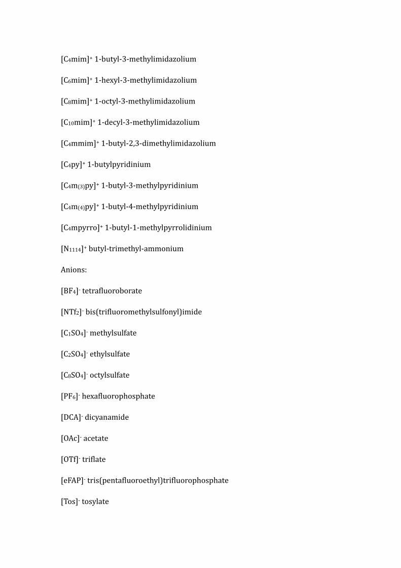
[C4mim]+ 1-butyl-3-methylimidazolium

[C6mim]+ 1-hexyl-3-methylimidazolium

[C8mim]+ 1-octyl-3-methylimidazolium

[C10mim]+ 1-decyl-3-methylimidazolium

[C4mmim]+ 1-butyl-2,3-dimethylimidazolium

[C4py]+ 1-butylpyridinium

[C4m(3)py]+ 1-butyl-3-methylpyridinium

[C4m(4)py]+ 1-butyl-4-methylpyridinium

[C4mpyrro]+ 1-butyl-1-methylpyrrolidinium

[N1114]+ butyl-trimethyl-ammonium

Anions:

[BF4]- tetrafluoroborate

[NTf2]- bis(trifluoromethylsulfonyl)imide

[C1SO4]- methylsulfate

[C2SO4]- ethylsulfate

[C8SO4]- octylsulfate

[PF6]- hexafluorophosphate

[DCA]- dicyanamide

[OAc]- acetate

[OTf]- triflate

[eFAP]- tris(pentafluoroethyl)trifluorophosphate

[Tos]- tosylate

NOMENCLATURE

Roman Letters:

𝐴 VFT equation parameter

𝐴0 parameter in eq. 6

𝑎 parameter in eq. 2

𝑎𝑖 parameter of group 𝑖

𝐵 VFT equation parameter

𝐵0 parameter in eq. 7

𝐵0′ parameter in eq. 7

𝑏𝑖 parameter of group 𝑖

𝐶 total number of components in UNIFAC-VISCO method

𝑐 concentration of the charge carriers

𝐷 self-diffusion coefficient (m2/s)

𝑑 parameter in eq. 1

𝑒0 elementary charge

𝑔𝑐𝐸 combinatorial contribution term in UNIFAC-VISCO method

𝑔𝑟𝐸 residual contribution term in UNIFAC-VISCO method

ℎ parameter in eq. 1

𝑘𝐵 Boltzmann constant (J/K)

𝑛 moles of the charge carriers

𝑛𝑖 total number of 𝑖th group present in the IL

𝑛𝑖,𝑘 total number of 𝑘th group present in component 𝑖

𝑀 number of data points

𝑁 total number

𝑁𝐴 Avogadro number (mol-1)

𝑄𝑘 group surface area parameter

𝑞𝑖 van der Waals’ surface area of component 𝑖

𝑟 effective radius

ℛ gas constant (J/mol·K)

𝑇 temperature (K)

𝑇0 VFT equation parameter

𝑇0′ parameter in eq. 8

𝑉 volume of the charge carriers present

𝑉𝑖 pure-component molar volume (m3/kmol)

𝑉𝑚 molar volume of ionic liquid (m3/kmol)

𝑊𝐴𝑚,𝑖 contribution of the 𝑚th-order group 𝑖

𝑊𝐵𝑚,𝑖 contribution of the 𝑚th-order group 𝑖

𝑊𝐵𝑚,𝑖′ contribution of the 𝑚th-order group 𝑖

𝑊𝑇0𝑚,𝑖 contribution of the 𝑚th-order group 𝑖

𝑥𝑖 mole fraction of the component 𝑖

𝑧 valence of the charge carrier

Greek Letters:

𝛼𝑚𝑛 interaction parameter between groups 𝑚 and 𝑛

𝛽𝑋 substituent constant

𝛾𝑚 residual activity coefficient

𝜃𝑖 molecular surface area fraction of component 𝑖

Θ𝑖 area fraction for group 𝑖

𝜎 conductivity (S/cm)

𝜎𝑒𝑥𝑝 conductivity experimentally measured

𝜎𝑐𝑎𝑙 conductivity calculated by our method

𝜎𝑖 conductivity of the pure component 𝑖

𝜎𝑋 conductivity of 𝑋-substituted IL

𝜎0 conductivity of methyl-substituted IL

𝜎𝑐𝑖 contribution of sub-structure 𝑖 on cations

𝜎𝑎𝑖 contribution of sub-structure 𝑖 on anions

𝜂 viscosity (mPa·s)

𝜂𝑐𝑎𝑙 calculated viscosity

𝜙𝑖 molecular volume fraction of component 𝑖

Ψ𝑚,𝑛 group interaction parameter

Λ molar conductivity (S·m2·mol-1)

REFERENCES

[1] P. Wasserscheid, T. Welton, Ionic Liquids in Synthesis, Wiley-VCH: Weinheim,

2003.

[2] M. Watanabe, M.L. Thomas, S. Zhang, K. Ueno, T. Yasuda, K. Dokko,

Application of Ionic Liquids to Energy Storage and Conversion Materials and

Devices, Chem. Rev. (2017). doi:10.1021/acs.chemrev.6b00504.

[3] K.-J. Wu, H. Luo, L. Yang, Structure-based model for prediction of electrical

conductivity of pure ionic liquids, AIChE J. 62 (2016) 3751–3762.

[4] J.M. Slattery, C. Daguenet, P.J. Dyson, T.J.S. Schubert, I. Krossing, How to

Predict the Physical Properties of Ionic Liquids: A Volume-Based Approach,

Angew. Chem. Int. Ed. 46 (2007) 5384–5388.

[5] M.G. Bogdanov, B. Iliev, W. Kantlehner, The Residual Volume Approach II:

Simple Prediction of Ionic Conductivity of Ionic Liquids, Z. Naturforsch. 64b

(2009) 756–764.

[6] R.L. Gardas, J.A.P. Coutinho, Group contribution methods for the prediction of

thermophysical and transport properties of ionic liquids, AIChE J. 55 (2009)

1274–1290.

[7] F. Gharagheizi, P. Ilani-Kashkouli, M. Sattari, A.H. Mohammadi, D.

Ramjugernath, D. Richon, Development of a LSSVM-GC model for estimating

the electrical conductivity of ionic liquids, Chem. Eng. Res. Des. 92 (2014) 66–

79.

[8] A.P. Abbott, Application of Hole Theory to the Viscosity of Ionic and Molecular

Liquids, ChemPhysChem. 5 (2004) 1242–1246.

[9] H. Zhao, Z.-C. Liang, F. Li, An improved model for the conductivity of

room-temperature ionic liquids based on hole theory, J. Mol. Liq. 149 (2009)

55–59.

[10] H. Matsuda, H. Yamamoto, K. Kurihara, K. Tochigi, Computer-aided reverse

design for ionic liquids by QSPR using descriptors of group contribution type

for ionic conductivities and viscosities, Fluid Phase Equilib. 261 (2007) 434–

443.

[11] K. Tochigi, H. Yamamoto, Estimation of ionic conductivity and viscosity of ionic

liquids using a QSPR model, J. Phys. Chem. C. 111 (2007) 15989–15994.

[12] Q. Dong, C.D. Muzny, A. Kazakov, V. Diky, J.W. Magee, J.A. Widegren, R.D.

Chirico, K.N. Marsh, M. Frenkel, ILThermo: A free-access web database for

thermodynamic properties of ionic liquids, J. Chem. Eng. Data. 52 (2007)

1151–1159.

[13] J. Vila, B. Fernández-Castro, E. Rilo, J. Carrete, M. Domínguez-Pérez, J.R.

Rodríguez, M. García, L.M. Varela, O. Cabeza, Liquid-solid-liquid phase

transition hysteresis loops in the ionic conductivity of ten imidazolium-based

ionic liquids, Fluid Phase Equilib. 320 (2012) 1–10.

[14] J. Vila, P. Ginés, J.M. Pico, C. Franjo, E. Jiménez, L.M. Varela, O. Cabeza,

Temperature dependence of the electrical conductivity in EMIM-based ionic

liquids: Evidence of Vogel-Tamman-Fulcher behavior, Fluid Phase Equilib. 242

(2006) 141–146.

[15] I. Bandrés, D.F. Montaño, I. Gascón, P. Cea, C. Lafuente, Study of the

conductivity behavior of pyridinium-based ionic liquids, Electrochim. Acta. 55

(2010) 2252–2257.

[16] H. Tokuda, S. Tsuzuki, M.A.B.H. Susan, K. Hayamizu, M. Watanabe, How ionic

are room-temperature ionic liquids? An indicator of the physicochemical

properties, J. Phys. Chem. B. 110 (2006) 19593–19600.

[17] Y.O. Andriyko, W. Reischl, G.E. Nauer, Trialkyl-Substituted Imidazolium-Based

Ionic Liquids for Electrochemical Applications: Basic Physicochemical

Properties, J. Chem. Eng. Data. 54 (2009) 855–860.

[18] H. Ning, M. Hou, Q. Mei, Y. Liu, D. Yang, B. Han, The physicochemical

properties of some imidazolium-based ionic liquids and their binary mixtures,

Sci. China Chem. 55 (2012) 1509–1518.

[19] M. Kanakubo, K.R. Harris, N. Tsuchihashi, K. Ibuki, M. Ueno, Temperature and

pressure dependence of the electrical conductivity of the ionic liquids

1-methyl-3-octylimidazolium hexafluorophosphate and

1-methyl-3-octylimidazolium tetrafluoroborate, Fluid Phase Equilib. 261 (2007)

414–420.

[20] S. Aparicio, R. Alcalde, B. Garcia, J.M. Leal, High-Pressure Study of the

Methylsulfate and Tosylate Imidazolium Ionic Liquids, J. Phys. Chem. B. 113

(2009) 5593–5606.

[21] B.E. Mbondo Tsamba, S. Sarraute, M. Traïkia, P. Husson, Transport Properties

and Ionic Association in Pure Imidazolium-Based Ionic Liquids as a Function of

Temperature, J. Chem. Eng. Data. 59 (2014) 1747–1754.

[22] Y.H. Yu, A.N. Soriano, M.H. Li, Heat capacities and electrical conductivities of

1-n-butyl-3-methylimidazolium-based ionic liquids, Thermochim. Acta. 482

(2009) 42–48.

[23] A.B. Pereiro, J.M.M. Araújo, F.S. Oliveira, C.E.S. Bernardes, J.M.S.S. Esperanca,

J.N.C. Lopes, I.M. Marrucho, L.P.N. Rebelo, Inorganic salts in purely ionic liquid

media: the development of high ionicity ionic liquids (HIILs), Chem. Commun.

48 (2012) 3656–3658.

[24] O. Cabeza, J. Vila, E. Rilo, M. Domínguez-Pérez, L. Otero-Cernadas, E.

López-Lago, T. Méndez-Morales, L.M. Varela, Physical properties of aqueous

mixtures of the ionic 1-ethl-3-methyl imidazolium octyl sulfate: A new ionic

rigid gel, J. Chem. Thermodyn. 75 (2014) 52–57.

[25] Y.H. Yu, A.N. Soriano, M.H. Li, Heat capacities and electrical conductivities of

1-ethyl-3-methylimidazolium-based ionic liquids, J. Chem. Thermodyn. 41

(2009) 103–108.

[26] O. Zech, A. Stoppa, R. Buchner, W. Kunz, The Conductivity of

Imidazolium-Based Ionic Liquids from (248 to 468) K. B. Variation of the Anion,

J. Chem. Eng. Data. 55 (2010) 1774–1778.

[27] N. Zec, M. Bešter-Rogač, M. Vraneš, S. Gadžurić, Physicochemical properties

of (1-butyl-1-methylpyrrolydinium dicyanamide + γ-butyrolactone) binary

mixtures, J. Chem. Thermodyn. 91 (2015) 327–335.

[28] J.-G. Li, Y.-F. Hu, S. Ling, J.-Z. Zhang, Physicochemical Properties of [C6mim][PF6]

and [C6mim][(C2F5)3PF3] Ionic Liquids, J. Chem. Eng. Data. 56 (2011) 3068–

3072.

[29] J.A. Widegren, E.M. Saurer, K.N. Marsh, J.W. Magee, Electrolytic conductivity

of four imidazolium-based room-temperature ionic liquids and the effect of a

water impurity, J. Chem. Thermodyn. 37 (2005) 569–575.

[30] S. Papović, M. Vraneš, S. Gadžurić, A comprehensive study of {γ-butyrolactone

+ 1-methyl-3-propylimidazolium bis(trifluoromethylsulfonyl)imide} binary

mixtures, J. Chem. Thermodyn. 91 (2015) 360–368.

[31] Q.-G. Zhang, Y. Wei, S.-S. Sun, C. Wang, M. Yang, Q.-S. Liu, Y.-A. Gao, Study on

Thermodynamic Properties of Ionic Liquid N-Butyl-3-methylpyridinium

Bis(trifluoromethylsulfonyl)imide, J. Chem. Eng. Data. 57 (2012) 2185–2190.

[32] Q.-S. Liu, P.-P. Li, U. Welz-Biermann, X.-X. Liu, J. Chen, Density, Electrical

Conductivity, and Dynamic Viscosity of N-Alkyl-4-methylpyridinium

Bis(trifluoromethylsulfonyl)imide, J. Chem. Eng. Data. 57 (2012) 2999–3004.

[33] M. Kanakubo, K.R. Harris, N. Tsuchihashi, K. Ibuki, M. Ueno, Temperature and

Pressure Dependence of the Electrical Conductivity of

1-Butyl-3-methylimidazolium Bis(trifluoromethanesulfonyl)amide, J. Chem.

Eng. Data. 60 (2015) 1495–1503.

[34] M. Vranes, S. Dozic, V. Djeric, S. Gadzuric, Physicochemical Characterization of

1-Butyl-3-methylimidazolium and 1-Butyl-1-methylpyrrolidinium

Bis(trifluoromethylsulfonyl)imide, J. Chem. Eng. Data. 57 (2012) 1072–1077.

[35] Q.G. Zhang, S.S. Sun, S. Pitula, Q.S. Liu, U. Welz-Biermann, J.J. Zhang, Electrical

conductivity of solutions of ionic liquids with methanol, ethanol, acetonitrile,

and propylene carbonate, J. Chem. Eng. Data. 56 (2011) 4659–4664.

[36] A. Nazet, S. Sokolov, T. Sonnleitner, T. Makino, M. Kanakubo, R. Buchner,

Densities, Viscosities, and Conductivities of the Imidazolium Ionic Liquids

[Emim][Ac], [Emim][FAP], [Bmim][BETI], [Bmim][FSI], [Hmim][TFSI], and

[Omim][TFSI], J. Chem. Eng. Data. 60 (2015) 2400–2411.

[37] J.M.M. Araújo, A.B. Pereiro, F. Alves, I.M. Marrucho, L.P.N. Rebelo, Nucleic

acid bases in 1-alkyl-3-methylimidazolium acetate ionic liquids: A

thermophysical and ionic conductivity analysis, J. Chem. Thermodyn. 57 (2013)

1–8.

[38] M. Kanakubo, K.R. Harris, N. Tsuchihashi, K. Ibuki, M. Ueno, Effect of Pressure

on Transport Properties of the Ionic Liquid 1-Butyl-3-methylimidazolium

Hexafluorophosphate, J. Phys. Chem. B. 111 (2007) 2062–2069.

[39] K.R. Harris, M. Kanakubo, N. Tsuchihashi, K. Ibuki, M. Ueno, Effect of pressure

on the transport properties of ionic liquids: 1-alkyl-3-methylimidazolium salts.,

J. Phys. Chem. B. 112 (2008) 9830–9840.

[40] N. Zhao, J. Jacquemin, R. Oozeerally, V. Degirmenci, New Method for the

Estimation of Viscosity of Pure and Mixtures of Ionic Liquids Based on the

UNIFAC–VISCO Model, J. Chem. Eng. Data. 61 (2016) 2160–2169.

[41] N. Zhao, R. Oozeerally, V. Degirmenci, Z. Wagner, M. Bendová, J. Jacquemin,

New Method Based on the UNIFAC–VISCO Model for the Estimation of Ionic

Liquids Viscosity Using the Experimental Data Recommended by

Mathematical Gnostics, J. Chem. Eng. Data. 61 (2016) 3908–3921.

[42] S. Bulut, P. Eiden, W. Beichel, J.M. Slattery, T.F. Beyersdorff, T.J.S. Schubert, I.

Krossing, Temperature Dependence of the Viscosity and Conductivity of Mildly

Functionalized and Non-Functionalized [Tf2N]− Ionic Liquids, ChemPhysChem.

12 (2011) 2296–2310.

[43] J. Jacquemin, P. Nancarrow, D.W. Rooney, M.F. Costa Gomes, P. Husson, V.

Majer, A.A.H. Padua, C. Hardacre, Prediction of Ionic Liquid Properties. II.

Volumetric Properties as a Function of Temperature and Pressure, J. Chem.

Eng. Data. 53 (2008) 2133–2143.

[44] J. Jacquemin, R. Ge, P. Nancarrow, D.W. Rooney, M.F. Costa Gomes, A.A.H.

Pádua, C. Hardacre, Prediction of Ionic Liquid Properties. I. Volumetric

Properties as a Function of Temperature at 0.1 MPa, J. Chem. Eng. Data. 53

(2008) 716–726.

[45] Y. Wang, W. Hao, J. Jacquemin, P. Goodrich, M. Atilhan, M. Khraisheh, D.

Rooney, J. Thompson, Enhancing Liquid-Phase Olefin-Paraffin Separations

Using Novel Silver-Based Ionic Liquids, J. Chem. Eng. Data. 60 (2015) 28–36.

[46] D.W. Marquardt, An Algorithm for Least-Squares Estimation of Nonlinear

Parameters, J. Soc. Indust. Appl. Math. 11 (1963) 431–441.

[47] P.D.A. Bastos, F.S. Oliveira, L.P.N. Rebelo, A.B. Pereiro, I.M. Marrucho,

Separation of azeotropic mixtures using high ionicity ionic liquids based on

1-ethyl-3-methylimidazolium thiocyanate, Fluid Phase Equilib. 389 (2015) 48–

54.

Table 1. An overview of the experimental conductivity data used to establish the

UNIFAC-CONDUCT model in this work

Ionic Liquid T / K No. of data points σ / S·m-1 Ref.

[C10mim][BF4] 263.1-353.1 34 0.00236-0.409 [13]

[C2mim][BF4] 258.1-433.1 36 0.245-12.68 [14]

[C4m(3)py][BF4] 278.15-338.15 25 0.0495-1.193 [15]

[C4m(4)py][BF4] 278.15-338.15 25 0.0381-1.211 [15]

[C4mim][BF4] 263.15-373.15 10 0.036-3.4 [16]

[C4mmim][BF4] 303.15-368.15 14 0.0758-1.5511 [17]

[C4py][BF4] 278.15-338.15 25 0.0591-1.311 [15]

[C6mim][BF4] 303-333 7 0.1598-0.576 [18]

[C8mim][BF4] 273.23-353.21 57 0.00961-0.5806 [19]

[C1mim][C1SO4] 278.15-368.15 10 0.1449-2.53 [20]

[C2mim][C1SO4] 298.15-343.15 6 0.602-2.336 [21]

[C4mim][C1SO4] 303.2-353.2 11 0.217-1.667 [22]

[C2mim][C2SO4] 298.15-323.15 6 0.3798-1.0005 [23]

[C2mim][C8SO4] 258.1-373.1 24 0.002-0.731 [24]

[C2mim][DCA] 293.2-353.2 11 1.89-6.86 [25]

[C4m(3)py][DCA] 288.15-338.15 21 0.526-2.91 [15]

[C4mim][DCA] 248.15-468.15 23 0.0483-14.54 [26]

[C4mpyrro][DCA] 273.15-323.15 11 0.523-2.529 [27]

[C6mim][eFAP] 293.15-343.15 11 0.1303-0.769 [28]

[C1mim][NTf2] 293.15-373.15 7 0.75-4.3 [16]

[C2mim][NTf2] 288.15-323.15 5 0.644-1.789 [29]

[C3mim][NTf2] 293.15-323.15 7 0.355-0.923 [30]

[C4m(3)py][NTf2] 278.15-353.15 16 0.1-1.437 [31]

[C4m(4)py][NTf2] 278.15-338.15 13 0.124-1.207 [32]

[C4mim][NTf2] 273.15-353.17 58 0.1181-1.796 [33]

[C4mpyrro][NTf2] 298.15-353.15 56 0.277-1.492 [34]

[C4py][NTf2] 283.15-313.15 10 0.15-0.542 [35]

Table 1. Continued …

Ionic Liquid T / K No. of data points σ / S·m-1 Ref.

[C6mim][NTf2] 278.15-468.15 20 0.07762-5.237 [36]

[C8mim][NTf2] 273.15-468.15 29 0.03083-4.029 [36]

[N1114][NTf2] 263.15-373.15 10 0.021-1.8 [16]

[C2mim][OAc] 298.15-418.15 13 0.2776-6.917 [36]

[C4mim][OAc] 283.15-323.15 9 0.0131-0.221 [37]

[C2mim][OTf] 293.2-353.2 11 0.834-3.51 [25]

[C4mim][OTf] 268.15-468.15 21 0.0539-7.5 [26]

[C4mim][PF6] 298.14-353.12 17 0.1379-1.1345 [38]

[C6mim][PF6] 273.21-353.18 48 0.0075-0.62102 [39]

[C8mim][PF6] 273.2-353.17 57 0.00325-0.3598 [19]

[C2mim][Tos] 278.15-368.15 10 0.0183-1.173 [20]

Table 2. Experimental Data Collected from Bastos et al. [47] Used During the Prediction

of the Conductivity of the (x[C2mim][DCA] + (1-x)[C2mim][SCN]) Binary Mixture

Temp. (K)

x=0.2397 x=0.4888 x=0.7415

𝜎𝜎𝑒𝑒𝑒𝑒𝑒𝑒

(S·cm-1)

𝜎𝜎𝑐𝑐𝑐𝑐𝑐𝑐

(S·cm-1)

𝜎𝜎𝑒𝑒𝑒𝑒𝑒𝑒

(S·cm-1)

𝜎𝜎𝑐𝑐𝑐𝑐𝑐𝑐

(S·cm-1)

𝜎𝜎𝑒𝑒𝑒𝑒𝑒𝑒

(S·cm-1)

𝜎𝜎𝑐𝑐𝑐𝑐𝑐𝑐

(S·cm-1)

298.15 0.0241 0.0242 0.0251 0.0241 0.0268 0.0248

303.15 0.0276 0.0278 0.0289 0.0276 0.0305 0.0282

308.15 0.0314 0.0317 0.0327 0.0313 0.0345 0.0319

313.15 0.0356 0.0359 0.0367 0.0353 0.0387 0.0359

318.15 0.0402 0.0404 0.0415 0.0396 0.0433 0.0400

323.15 0.0448 0.0451 0.0462 0.0441 0.0481 0.0445

RAAD% (each set) 0.71% 4.19% 7.50%

RAAD% (global) 4.13%

Figure 1. Comparison of experimental (𝜎𝜎𝑒𝑒𝑒𝑒𝑒𝑒) and evaluated (𝜎𝜎𝑐𝑐𝑐𝑐𝑐𝑐) conductivity data for pure

ILs by using a) method 1; b) method 2; and c) method 3 as described in sections 2.2, 2.3 and

2.4, respectively.

Figure 2. Comparison of the temperature dependence on the conductivity data of the

[C4mpyrro][NTf2] from the literature [34] and the UNIFAC-CONDUCT model approaches

investigated during this work.

Figure 3. Comparison of the effect of anion structure on the conductivity data of [C4mim]+-

based ILs at 298.15 K from the literature [16,26,33,37,38] and the UNIFAC-CONDUCT model

approaches investigated during this work.

Figure 4. Comparison of the effect of cation structure on the conductivity data of [NTf2]--based

ILs at 298.15 K from the literature [16,29,30,33,34,36] and the UNIFAC-CONDUCT model

approaches investigated during this work.

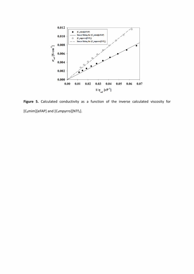
Figure 5. Calculated conductivity as a function of the inverse calculated viscosity for

[C6mim][eFAP] and [C4mpyrro][NTf2].

Figure 6. Relative deviations between the purely predicted values (𝜎𝜎𝑐𝑐𝑐𝑐𝑐𝑐) and the experimental

conductivity data (𝜎𝜎𝑒𝑒𝑒𝑒𝑒𝑒) of the binary system (x[C2mim][DCA] + (1-x)[C2mim][SCN]) from [47]

as a function of temperature (298.15 K – 323.15 K) and composition: +, x=0.2397; ○, x=0.4888;

□, x=0.7415.

Supporting Information

The Development of the UNIFAC-CONDUCT Model as a Novel Approach

for the Estimation of the Conductivity of Pure Ionic Liquids

Nan Zhao1, Johan Jacquemin1,2,*

1 School of Chemistry and Chemical Engineering, Queen’s University Belfast, Belfast,

BT9 5AG, U.K. 2 Universite Francois Rabelais, Laboratoire PCM2E, Parc de Grandmont 37200 Tours, France

Table S1. Parameters of effective molar volume for cations and anions

Ion D0

cm3·mol-1

D1

cm3·mol-1·K-1

D2

cm3·mol-1·K-2 RAAD

[C1mim]+ 84.61 0.0367 7.72E-05 0 [C2mim]+ 100.25 0.0656 4.57E-05 2.40E-04 [C3mim]+ 117.14 0.0445 1.18E-03 0 [C4mim]+ 134.11 0.0927 -2.99E-05 2.26E-03 [C6mim]+ 168.60 0.1131 4.93E-05 7.83E-04 [C8mim]+ 202.14 0.1852 -3.53E-04 3.02E-03 [C10mim]+ 236.36 0.1748 1.76E-04 0

[C4mmim]+ 147.30 0.0974 6.75E-05 1.97E-03 [C4py]+ 129.98 0.0799 2.60E-05 4.17E-03

[C4m(3)py]+ 146.72 0.0900 8.61E-05 3.06E-04 [C4m(4)py]+ 145.73 0.0907 3.82E-05 1.50E-03

[C4mpyrro]+ 145.15 0.0929 -7.70E-06 2.75E-03 [N1114]+ 127.14 0.0772 6.94E-05 0 [BF4]- 53.75 0.0258 -3.40E-05 1.31E-03

[C1SO4]- 72.32 0.0429 -8.86E-05 1.76E-03 [NTf2]- 157.60 0.1043 5.05E-05 0 [PF6]- 72.85 0.0363 -3.84E-05 1.93E-03 [DCA]- 59.59 0.0237 4.49E-05 1.95E-03 [Tos]- 130.89 0.0582 -1.21E-04 0 [OAc]- 54.44 0.0237 -7.98E-05 4.97E-04 [OTf]- 89.02 0.0628 -3.66E-05 7.01E-03

[eFAP]- 225.74 0.1651 -2.71E-06 1.89E-03 [C2SO4]- 90.72 0.0394 -1.66E-05 0 [C8SO4]- 192.36 0.0741 3.15E-04 0

Table S2. The UNIFAC-CONDUCT volume (𝑅𝑅 ) and surface area (𝑄𝑄 ) parameters for cations and anions

Ion R Q [C1mim]+ 4.1183 3.4946 [C2mim]+ 4.7608 4.0087 [C3mim]+ 5.4342 4.5473 [C4mim]+ 6.1040 5.0832 [C6mim]+ 7.4623 6.1698 [C8mim]+ 8.8143 7.2515 [C10mim]+ 10.1662 8.3329

[C4mmim]+ 6.7595 5.6076 [C4py]+ 5.9737 4.9790

[C4m(3)py]+ 6.6210 5.4968 [C4m(4)py]+ 6.6310 5.5048

[C4mpyrro]+ 6.6061 5.4849 [N1114]+ 5.6947 4.7558 [BF4]- 2.2421 1.9937

[C1SO4]- 3.1995 2.7596 [NTf2]- 6.7937 5.6350 [PF6]- 3.1900 2.7520 [DCA]- 2.5346 2.2277 [Tos]- 5.7510 4.8008 [OAc]- 2.2192 1.9754 [OTf]- 3.9625 3.3700

[eFAP]- 9.8900 8.1120 [C2SO4]- 3.8506 3.2805 [C8SO4]- 7.9095 6.5276

Table S3. Binary interaction parameters 𝛼𝛼𝑚𝑚𝑚𝑚 used in the first method and second method

m n 𝜶𝜶𝒎𝒎𝒎𝒎 𝜶𝜶𝒎𝒎𝒎𝒎

[C10mim]+ [BF4]- 77.85 -410.46

[C1mim]+ [NTf2]- -391.35 931.41

[C1mim]+ [C1SO4]- -158.30 -54.69

[C2mim]+ [BF4]- -222.19 -130.81

[C2mim]+ [C1SO4]- 566.37 -354.46

[C2mim]+ [NTf2]- -322.07 1978.2

[C2mim]+ [OAc]- -611.17 6394.8

[C2mim]+ [OTf]- 1717.4 -465.92

[C2mim]+ [DCA]- 9765.3 -260.54

[C2mim]+ [C2SO4]- 355.51 423.56

[C2mim]+ [C8SO4]- -423.54 2156.2

[C2mim]+ [Tos]- 35.38 -13.35

[C3mim]+ [NTf2]- 67.96 -111.31

[C4m(4)py]+ [BF4]- -678.30 1116.6

[C4m(4)py]+ [NTf2]- 65.77 -9.79

[C4m(3)py]+ [DCA]- 4174.7 -336.84

[C4m(3)py]+ [NTf2]- 702.97 -262.88

[C4m(3)py]+ [BF4]- -660.43 1990.6

[C4mim]+ [BF4]- -0.06 -464.73

[C4mim]+ [C1SO4]- 112.45 -365.32

[C4mim]+ [NTf2]- 322.36 -228.33

[C4mim]+ [PF6]- 1248.42 -544.06

[C4mim]+ [OAc]- 4669.6 -712.86

[C4mim]+ [OTf]- -280.50 -14.04

[C4mim]+ [DCA]- 361.00 -291.30

[C4mmim]+ [BF4]- -105.01 -768.66

Table S3. Continued …

m n 𝜶𝜶𝒎𝒎𝒎𝒎 𝜶𝜶𝒎𝒎𝒎𝒎

[C4mpyrro]+ [NTf2]- -127.47 -29.34

[C4mpyrro]+ [DCA]- -208.95 -53.51

[C4py]+ [BF4]- -404.47 7644.6

[C4py]+ [NTf2]- 86.82 417.64

[C6mim]+ [BF4]- -155.98 -414.47

[C6mim]+ [PF6]- 2912.7 -584.72

[C6mim]+ [eFAP]- 439.06 -274.24

[C6mim]+ [NTf2]- -251.08 415.53

[C8mim]+ [NTf2]- 80.21 36.46

[C8mim]+ [BF4]- -443.32 29.73

[C8mim]+ [PF6]- -506.07 1351.0

[N1114]+ [NTf2]- -3.97 -9.63

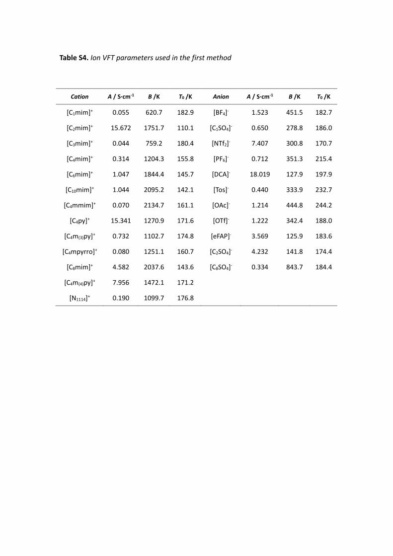
Table S4. Ion VFT parameters used in the first method

Cation A / S·cm-1 B /K T0 /K Anion A / S·cm-1 B /K T0 /K

[C1mim]+ 0.055 620.7 182.9 [BF4]- 1.523 451.5 182.7

[C2mim]+ 15.672 1751.7 110.1 [C1SO4]- 0.650 278.8 186.0

[C3mim]+ 0.044 759.2 180.4 [NTf2]- 7.407 300.8 170.7

[C4mim]+ 0.314 1204.3 155.8 [PF6]- 0.712 351.3 215.4

[C6mim]+ 1.047 1844.4 145.7 [DCA]- 18.019 127.9 197.9

[C10mim]+ 1.044 2095.2 142.1 [Tos]- 0.440 333.9 232.7

[C4mmim]+ 0.070 2134.7 161.1 [OAc]- 1.214 444.8 244.2

[C4py]+ 15.341 1270.9 171.6 [OTf]- 1.222 342.4 188.0

[C4m(3)py]+ 0.732 1102.7 174.8 [eFAP]- 3.569 125.9 183.6

[C4mpyrro]+ 0.080 1251.1 160.7 [C2SO4]- 4.232 141.8 174.4

[C8mim]+ 4.582 2037.6 143.6 [C8SO4]- 0.334 843.7 184.4

[C4m(4)py]+ 7.956 1472.1 171.2

[N1114]+ 0.190 1099.7 176.8

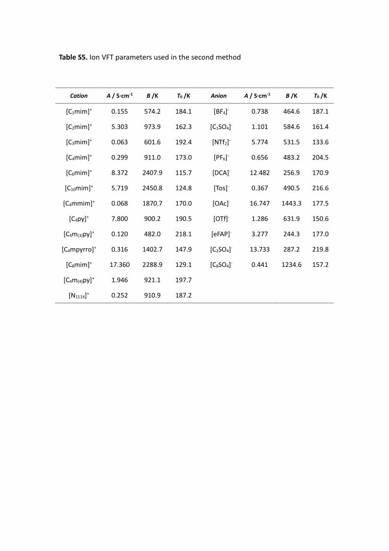
Table S5. Ion VFT parameters used in the second method

Cation A / S·cm-1 B /K T0 /K Anion A / S·cm-1 B /K T0 /K

[C1mim]+ 0.155 574.2 184.1 [BF4]- 0.738 464.6 187.1

[C2mim]+ 5.303 973.9 162.3 [C1SO4]- 1.101 584.6 161.4

[C3mim]+ 0.063 601.6 192.4 [NTf2]- 5.774 531.5 133.6

[C4mim]+ 0.299 911.0 173.0 [PF6]- 0.656 483.2 204.5

[C6mim]+ 8.372 2407.9 115.7 [DCA]- 12.482 256.9 170.9

[C10mim]+ 5.719 2450.8 124.8 [Tos]- 0.367 490.5 216.6

[C4mmim]+ 0.068 1870.7 170.0 [OAc]- 16.747 1443.3 177.5

[C4py]+ 7.800 900.2 190.5 [OTf]- 1.286 631.9 150.6

[C4m(3)py]+ 0.120 482.0 218.1 [eFAP]- 3.277 244.3 177.0

[C4mpyrro]+ 0.316 1402.7 147.9 [C2SO4]- 13.733 287.2 219.8

[C8mim]+ 17.360 2288.9 129.1 [C8SO4]- 0.441 1234.6 157.2

[C4m(4)py]+ 1.946 921.1 197.7

[N1114]+ 0.252 910.9 187.2

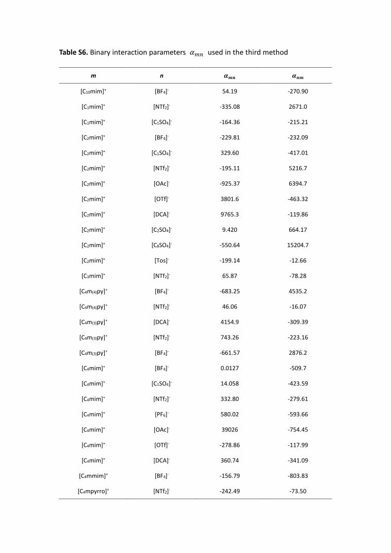
Table S6. Binary interaction parameters 𝛼𝛼𝑚𝑚𝑚𝑚 used in the third method

m n 𝜶𝜶𝒎𝒎𝒎𝒎 𝜶𝜶𝒎𝒎𝒎𝒎

[C10mim]+ [BF4]- 54.19 -270.90

[C1mim]+ [NTf2]- -335.08 2671.0

[C1mim]+ [C1SO4]- -164.36 -215.21

[C2mim]+ [BF4]- -229.81 -232.09

[C2mim]+ [C1SO4]- 329.60 -417.01

[C2mim]+ [NTf2]- -195.11 5216.7

[C2mim]+ [OAc]- -925.37 6394.7

[C2mim]+ [OTf]- 3801.6 -463.32

[C2mim]+ [DCA]- 9765.3 -119.86

[C2mim]+ [C2SO4]- 9.420 664.17

[C2mim]+ [C8SO4]- -550.64 15204.7

[C2mim]+ [Tos]- -199.14 -12.66

[C3mim]+ [NTf2]- 65.87 -78.28

[C4m(4)py]+ [BF4]- -683.25 4535.2

[C4m(4)py]+ [NTf2]- 46.06 -16.07

[C4m(3)py]+ [DCA]- 4154.9 -309.39

[C4m(3)py]+ [NTf2]- 743.26 -223.16

[C4m(3)py]+ [BF4]- -661.57 2876.2

[C4mim]+ [BF4]- 0.0127 -509.7

[C4mim]+ [C1SO4]- 14.058 -423.59

[C4mim]+ [NTf2]- 332.80 -279.61

[C4mim]+ [PF6]- 580.02 -593.66

[C4mim]+ [OAc]- 39026 -754.45

[C4mim]+ [OTf]- -278.86 -117.99

[C4mim]+ [DCA]- 360.74 -341.09

[C4mmim]+ [BF4]- -156.79 -803.83

[C4mpyrro]+ [NTf2]- -242.49 -73.50

Table S6. Continued …

m n 𝜶𝜶𝒎𝒎𝒎𝒎 𝜶𝜶𝒎𝒎𝒎𝒎

[C4mpyrro]+ [DCA]- -428.18 -291.61

[C4py]+ [BF4]- -441.1 18057

[C4py]+ [NTf2]- 64.51 240.96

[C6mim]+ [BF4]- -64.98 -161.37

[C6mim]+ [PF6]- 1399.7 -428.91

[C6mim]+ [eFAP]- 712.20 -124.31

[C6mim]+ [NTf2]- -228.61 1279.2

[C8mim]+ [NTf2]- 65.22 -81.20

[C8mim]+ [BF4]- -473.02 39.35

[C8mim]+ [PF6]- -590.31 17735

[N1114]+ [NTf2]- -0.282 27.65

Table S7. Ion VFT parameters used in the third method

Cation A / S·cm-1 B /K T0 /K Anion A / S·cm-1 B /K T0 /K

[C1mim]+ 0.137 501.0 188.1 [BF4]- 1.340 577.7 170.0

[C2mim]+ 0.428 612.6 154.4 [C1SO4]- 3.932 1095.8 137.2

[C3mim]+ 0.033 405.3 218.8 [NTf2]- 1.963 253.7 156.7

[C4mim]+ 0.136 868.8 181.1 [PF6]- 3.347 976.4 161.9

[C6mim]+ 2.210 1143.2 174.6 [DCA]- 19.748 387.2 105.0

[C10mim]+ 0.723 1366.6 171.2 [Tos]- 0.606 828.2 205.0

[C4mmim]+ 0.020 1815.6 172.6 [OAc]- 0.421 731.6 206.3

[C4py]+ 4.604 870.6 193.7 [OTf]- 1.295 689.0 133.1

[C4m(3)py]+ 0.554 746.9 202.4 [eFAP]- 3.871 168.6 204.9

[C4mpyrro]+ 0.108 1576.9 147.4 [C2SO4]- 13.815 365.6 228.2

[C8mim]+ 0.400 1225.3 177.0 [C8SO4]- 0.814 1653.2 158.9

[C4m(4)py]+ 0.932 806.8 205.2

[N1114]+ 0.944 1130.4 179.6