The cost-e�ciency of Swedish Arable-Nitrogen

Abatement Policy

Mark Brady

Department of Economics,

Swedish University of Agricultural Sciences, 750 07 Uppsala, Sweden

June 18, 2002

Paper presented to World Congress of Environmental and Resource Economists,

Monterey, California, June 24 - 27 2002.

E-mail: mark.brady@ekon.slu.se

Abstract

The purpose of this article was to study the economics of Sweden's

scheme of 'multiple' arable nitrogen abatement instruments. A large-scale,

spatially distributed mathematical programming model that linked changes

in agricultural production practices to coastal nitrogen load was developed.

Actual abatement policy induced 21% abatement. A �rst-best solution to

21% abatement required increased concentration of commodity production

and remaining land to be farmed relatively more pro�tably. A second-best

solution required sparser production and less cost-e�ective commodity pro-

duction. Under actual policy, relative abatement was too high in the fertile

southern coastal regions than either of the benchmarks. The choice of ef-

�ciency benchmark was critical to de�ning 'cost-e�ective' policies. Abate-

ment could be increased without causing excessive ine�ciencies with a)

incentives that also steer crop choice decisions and b) increased relative

abatement in less pro�table regions. Coordination of environmental and

agricultural policy could o�er considerable e�ciency gains.

1

1 Introduction

Arable nitrogen emissions contribute to severe eutrophication of the Baltic and North

Seas (Wul� et al., 1990; Turner et al., 1999), accounting for around 35% of total coastal

load and 45% of the Swedish load (SNV, 1997, p. 80). The countries bordering the

Baltic (Sweden, Denmark, Germany, Finland, Poland, Latvia, Lithuania, Estonia and

Russia) have the common ambition of restoring water quality to what it was some

40 years ago and have, consequently, committed themselves to reducing the nitrogen

load by 50% of the 1987 level (The Helsinki Commission, HELCOM; North Sea Con-

ference/Paris Commission). A similarly ambitious target has been proposed for the

Swedish agricultural sector (e.g. Albertsson et al., 1999). To induce abatement Sweden

has introduced a comprehensive scheme of policy instruments that include a nitrogen

input tax, land management subsidies and land-use regulations. The economics of this

scheme is the subject of this paper.

Arable nitrogen enters water di�usely in the runo� (leachate) from rain or melting

snow and emission rates are related to location speci�c factors such as climate, soil

type, hydrology, etc., and the choice of agricultural production technology. It is partic-

ularly di�cult for policymakers to control because of the prohibitive cost of monitoring

di�use or non-point source (NPS) pollution by source (Braden and Segerson, 1993).

Given this information problem, the design of policies for controlling NPS pollution

tend to be based on factors that indirectly determine the level of emissions and are

observable at relatively low cost, rather than water quality per se (Gri�n and Brom-

ley, 1982; Shortle and Dunn, 1986; Huang and Uri, 1992; Feinerman and Choi, 1993;

Helfand and House, 1995).

To achieve cost-e�ective coastal nitrogen abatement (also the least-cost or cost-

e�cient solution) the marginal cost of reducing load needs to be equalized across all

pollution sources (Baumol, 1972), in this case across all units of arable land in the

Swedish Baltic watershed. Obtaining such a result given the state of our technology is

of course a utopian goal. Nevertheless three general classes of decisions faced by farmers

have been shown to in�uence the cost-e�ciency of arable NPS pollution abatement:

i) the level of variable inputs per hectare or the intensity of production, ii) the choice

of crop management practices and iii) the allocation of land on the extensive margin

(i.e. the area of land in production) (see Horan and Ribaudo, 1999, for a review).

The purpose of this article is to study the economics of the Swedish scheme of

actual policies which comprises i) a national (or single-rate) nitrogen fertilizer tax

2

ii) single-rate subsidies based on the area of alternative crop management practices

(AMPs), i.e. cover/catch-crop or spring-tillage and iii) regulations pertaining to the

management of set-a-side (fallow land) and land between growing seasons.

This scheme or package of policies is cause for concern for a number of reasons.

First, uniform or single-rate policies are not likely to meet the equi-marginal cost prin-

ciple for least-cost abatement because of spatial heterogeneity (Gri�n and Bromley,

1982; Shortle and Dunn, 1986; Braden et al., 1989). Secondly, economic incentives

change the relative pro�tability of alternative cropping possibilities and, therefore,

might invoke undesirable substitution e�ects on the extensive margin (Bouzaher et al.,

1992, 1995). Thirdly, it might simply be e�cient to retire land from intensive crop pro-

duction rather than subsidizing costly management practices to achieve environmental

goals (Wu and Segerson, 1995). Finally, indirect incentives created by agricultural

income support policies and attendant constraints on the production set (under the

Common Agricultural Policy�CAP) might have implications for de�ning an e�ciency

benchmark to compare policies against.

In Sweden and other EU countries area payments, which are a form of direct in-

come support, are an important determinant of land use decisions and thereby the

environmental impacts of agriculture (Ingersent et al., 1998; Swinbank, 1999). These

are collected by farmers for growing eligible crops (primarily intensively grown grains

and oilseed). Some price support also exists with attendant impacts on the intensity

of production (Stoate et al., 2001). Theoretically, this system could be replaced by

lump-sum or production neutral transfers to farmers to meet income goals.

The analysis is therefore based on two alternative cost-e�ciency benchmarks. The

�rst-best solution to an abatement target implies that agricultural and environmen-

tal policy can be coordinated (income support is replaced by lump-sum transfers),

whilst the second-best solution takes the current structure of agricultural support to

be given�costs re�ect farmers' private opportunity costs only. The economic proper-

ties of the actual solution were evaluated by comparing it with the second-best and

�rst-best solutions for en equivalent level of abatement. The implications for increasing

the current level of abatement were also considered.

The empirical study was restricted to arable land in Southern Sweden that is only

spread with chemical fertilizers (or 1.5 of a total 2.3 million hectares). The sub-artic

region of northern Sweden was omitted from the study because it contributes only

marginally to the Baltic nitrogen problem and to sector pro�ts. Livestock farms were

3

excluded from the analysis because stable manure is essentially a waste disposal prob-

lem and is subjected to regulations that do not impinge upon commercial nitrogen

management (Brady, 2002a). A deterministic modelling approach was also adopted

and therefore the stochastic nature of nitrogen emissions was ignored. This delimita-

tion could impact the results if the policy maker is sensitive to the annual variability

of emissions (Brady, 2002b). Due to the expanse and heterogeneity of the study-area

a spatially distributed mathematical programming model that linked changes in agri-

cultural production technologies to coastal nitrogen load was developed. The model

is a static deterministic optimization model of farmer behaviour. The model included

the following information on physical processes a) the relationship between choice of

crop, nitrogen intensity and crop management practice, and nitrogen leached below

the root-zone given soil type and climate zone, and b) the amount of leached nitrogen

and net coastal load after allowing for retention (losses during transport from the root

zone to the sea). It was calibrated to observed production activity levels in 1999 using

Positive Mathematical Programming (Appendix B), a method which avoids placing

arbitrary constraints on the solution set.

Mathematical programming models which integrate physical process models with

economic optimization models are commonly used to analyze water quality problems.

Integration can occur directly (Fleming and Adams, 1997; Vatn et al., 1997; Schou

et al., 2000) or by using data generated by such models to estimate physical response

functions (Bouzaher et al., 1995; Helfand and House, 1995; Gren, 1997). The latter

approach was considered most appropriate for this study because of the large size of

the study area (Shogren, 1993). A programming rather than econometric approach was

adopted because historical data relating emissions to production decisions at a suitably

low scale do not exist�detailed speci�cation of production relationships is crucial for

predicting the impacts of changes in production choices on emissions (Just and Antle,

1990). Further, econometric models are typically unsuited to modelling situations

where production choices are likely to stray outside of historically observed choices

(O'Callaghan, 1996; Shumway and Chang, 1977) as exempli�ed by introducing nitrogen

abatement measures. A simpli�ed analytical model was used to derive theoretical

results.

Though an enormous amount of work has been done on the nitrogen problem this

study is important because it considers an unusually large watershed and a scheme of

multiple policies rather than a single policy approache which is often the case (Huang

4

and LeBlanc, 1994; Helfand and House, 1995; Larson et al., 1996; Gren, 1997). The

study also considers a much larger degree of spatial heterogeneity than these studies

and therefore should render more reliable conclusions about the relative e�ciency of

national instruments for NPS pollution control.

Actual abatement policy induced 21% abatement compared with an unconstrained

baseline scenario. A �rst-best solution to a 21% target would require increased con-

centration of commodity production and land to be farmed relatively more e�ectively

(pro�tably). A second-best solution would require sparser production and thus less

cost-e�ective commodity production than induced by actual policy. Therefore second-

best abatement required relatively higher reductions in nitrogen intensity and a greater

area of pollution reducing management practices (catch crops and spring tillage) than

both the actual and �rst-best solutions. Consequently, relative abatement was too

high in the pro�table, southern coastal regions under actual policy than either of the

benchmarks.

The choice of e�ciency benchmark was critical to de�ning 'cost-e�ective' policies.

The nitrogen tax performed relatively well by both benchmarks, whereas subsidies to

AMPs were only second-best instruments that also produced signi�cant and undesir-

able substitution e�ects. To increase abatement without causing excessive increases

in cost-ine�ciencies will require a) incentives that also steer land allocation (crop

choice) decisions and b) an increase in relative abatement in less pro�table agricul-

tural regions. Coordination of nitrogen and agricultural policy could therefore o�er

considerable e�ciency gains from a broader economic perspective.

2 Economic model of agriculture and coastal nitrogen

pollution

I begin the analysis by presenting a spatially distributed, static and deterministic

economic optimization model of the actual policy situation confronted by farmers, who

are assumed to maximize pro�ts, followed by the second-best and �rst-best abatement

models. Finally, a simpli�ed theoretical model is used to derive analytical results.

The actual model links changes in the agricultural production technology to changes

in coastal nitrogen load. Physical characteristics considered explicitly in the model are

soil type, climate, land productivity and retention (nitrogen assimilated by the envi-

ronment during transport from arable soils to the coast). The crop mix and land

5

management practices (together referred to as land-use) can be varied, as well as at-

tendant nitrogen intensity. The solution to the problem is the choices of land-uses

and nitrogen intensities that maximize pro�ts given exogenously imposed environmen-

tal (i.e. nitrogen) and agricultural policy variables. Coastal load generated by this

solution is referred to as actual load.

The second-best policy evaluation model is derived by removing nitrogen policy

variables from the actual policy model and appending a load constraint that limits

coastal load to actual load. The solution to this problem is the cost of achieving

actual abatement if e�cient second-best instruments were implemented instead of

actual instruments. Measures available to reduce emissions are the possibility to;

change crop allocations (e.g. take land out of production, substitute to less polluting

crops, etc), reduce nitrogen application rates and adopt a pollution reducing alternative

management practices (AMPs), such as a catch crop or delayed tillage. The �rst-best

model is derived by removing agricultural policy variables from the second-best model

and the solution is the cost of achieving actual load if socially e�cient policies were

implemented.

2.1 Actual policy model

Farmers are assumed to allocate land Xrsjm (ha) and apply nitrogen Nrsjm (kg/ha)

to maximize pro�t (excluding annual sunk costs) subject to relevant production and

policy constraints. The subscript r ∈ R denotes the watershed/region (homogenous in

both climatic and production conditions), s ∈ S soil type, j ∈ J crop type and m ∈ M

crop management practice. Thus Xrsjm is the area of crop j managed with practice m

that is grown in region r on soil type s, and Nrsjm is attendant total nitrogen input.

The actual policy model is formulated as

max ΠA(Nrsjm, Xrsjm) =R∑

r=1

S∑s=1

J∑j=1

M∑m=1

[(pW

j + pCj − crjm)F(Nrsjm, Xrsjm) +

+(APrj + ESrjm −HCrsjm)Xrsjm − (w + tN )Nrsjm

](1)

Subject toJ∑

j=1

M∑m=1

Xrsjm ≤ Xrs ∀r (LAND, µrs) (2)

S∑s=1

J∑j=1

M∑m=1

γjiXrsjm ≤ 0 ∀i, r (CROP, νri) (3)

6

−S∑

s=1

K∑k=1

M∑m=1

Xrskm ≤ −0.1ρj

S∑s=1

J∑j=1

M∑m=1

Xrsjm ∀r

where ρj = 0, 1 and k ∈ K ⊂ J (SET-A-SIDE, τr) (4)S∑

s=1

M∑m=1

F(Nrsqm, Xrsqm) ≤ Qrq ∀q, r

where q ∈ Q ⊂ J (QUOTA, κrq) (5)

−S∑

s=1

J∑j=1

M∑m=1

σjmXrsjm ≤ −θrS∑

s=1

J∑j=1

M∑m=1

Xrsjm ∀r

where σjm = 0, 1 and θr = (0, 1) (GREEN, ωr) (6)S∑

s=1

Xrskm =S∑

s=1

σkmXrskm ∀r (ENV FALL, χr) (7)

and the coastal load generated by actual policy, ZA, is

ZA =R∑

r=1

S∑s=1

J∑j=1

M∑m=1

(1− αr)Z(Nrsjm, Xrsjm) (8)

and note that in this model load not a constraint on the model but is simply calculated

after the optimization. But in the second and �rst-best models it is used as a constraint.

The objective, (1), is to maximize total sector pro�ts where pWj is the world mar-

ket price1 of output, pCj is the CAP price premium, crjm is yield dependent cost, F

is the crop yield function, APrj is an area payment for eligible crops, ESrjm is an

environmental subsidy for adoption of AMPs, HCrsjm is hectare dependent cost, w is

the unit cost of applying nitrogen fertilizer and tN is a unit tax on nitrogen content.

The parameters of the yield function are assumed to be unique for each (rsjm) and

it is assumed to be concave in nitrogen intensity (FN > 0 and FNN < 0) and the

area in each crop (FX > 0 and FXX < 0�average yield decreases as area is expanded

because the most productive land is assumed to be put in production �rst).

For readability the constraints are annotated with a name and the Greek letter used

to denote the associated Lagrangian multiplier, since the L-function is not reproduced.

(2) and (3) are production constraints that de�ne what is technologically possible. (2)

are land constraints that restrict the area in production in each region and for each

soil type to the natural endowment, Xrs (ha). (3) are crop management or rotation

constraints which farmers generally adhere to for diversi�cation purposes or the control

of weeds, diseases and insects. The coe�cient γji is the minimum proportion of the

restricted crop i that can be grown in combination with other crops j (i 6= j) de�ned1Prices to Swedish produces are taken as given because Swedish commodity output is insigni�cant

relative to total EU and world market output, and as a member of the EU Sweden can not protect

domestic production from competition from other EU states.

7

by constraint i (e.g. crops with the coe�cient −1 must be grown on an equal or greater

area than those with coe�cient +1 and 0 implies that crop j does not satisfy rotational

requirement i).

CAP provisions are captured by (4) and (5). To collect area payments, farmers

are required to take an area of at least 10% of the area sown to eligible crops out of

production (referred to as set-a-side). The subscript k refers to a subset of crops that

satisfy the de�nition of set-aside (i.e. fallow, energy or other non-food/fodder crops).

For eligible crops ρj = 1 and is otherwise zero. Output can be limited by quotas in

the event of price support (i.e. sugarbeets). The subscript q in (5) refers to a subset of

crops that are subject to quota restrictions and Qrq (kg) is the regional output quota.

Nitrogen regulations require that the proportion of winter-green land, (6),�land

that is not considered to be bare over the autumn/winter months�is not less than

θr = (0, 1) where σj,m = 0 or 1 indicates whether a particular land-use is considered

winter-green. Set-a-side, (7), must also be covered with a winter-green or cover crop.

Finally, negative levels of the choice variables are not permitted (not shown).

Coastal load generated by the solution to the actual policy problem, ZA, is cal-

culated by (8). The emissions (leaching) production function, Z, determines nitrogen

emissions by region, soil type and land-use given nitrogen intensity, and is assumed to

be convex in nitrogen intensity (ZN > 0 and ZNN > 0)�emissions increase exponen-

tially with intensity ceteris paribus) and land area (ZX > 0 and ZXX > 0)�marginal

land leaches more than highly productive land ceteris paribus). On its way to the

coast some fraction of leached nitrate is assimilated by the environment. These losses

are captured by the retention parameter, αr = [0, 1], where (1− αr) is the proportion

of leachate actually reaching the coast.

Whilst there are in principle two types of choices, land-use and nitrogen intensity,

the necessary conditions are quite di�erent for crops a�ected by the CAP. The �rst

order Kuhn-Tucker conditions (FOC) are therefore presented according to the following

categorizations: 1) other crops not a�ected by the CAP ; 2) crops eligible for CAP

support ; 3) quota restricted crops; and 4) set-a-side.

To begin the analysis as clearly as possible and with familiar conditions I present the

FOC for a hypothetical unfettered market solution where exogenous policy variables

are ignored. To simplify notation the j, m, r and s subscripts are suppressed on decision

variables and partial derivatives are subscripted (e.g. FN ≡ ∂F/∂Nrsjm for all jmrs,

8

is the change in yield given a change in nitrogen intensity)

NU : MVPN = w (9)

XU : MVPX = OL (10)

where MVPN ≡ [pWj − crjm]FN is the marginal value product of nitrogen application;

MVPX ≡ [pWj − crjm](F + FXX) is the marginal value product of arable land; and

OLrsjm ≡ HCrsjm+µrs+∑I

i νriγji is the private opportunity cost of land-use choices,

where µrs is the shadow price of the limited area of land and νri the implicit cost of

crop management constraints. In an unfettered market farmers apply nitrogen until

the MVP of nitrogen input is equal to its cost; and increase the area in a particular

land-use until the MVP of putting more land in production is equal to the private

opportunity cost of the land-use choice. If µrs = 0 the land constraint is not binding

and not all arable land will be put in production�land not in production or idled

land is assumed to generate only background leaching, the rate of which cannot (by

assumption) be a�ected by farmers' choices.

The FOCs for the actual policy solution now follow in the order of the categoriza-

tions given above.

NO : MVPN = w + tN (11)

XO : MVPX + ESrjm = OL + ωr(θr − σjm) (12)

where ωr is the imputed cost of the green-land constraint. A nitrogen tax reduces

pro�t maximizing intensity because FNN < 0. The environmental subsidy provides an

incentive to introduce the subsidized land-use�crop as well as management practice.

An AMP will not be adopted unless the subsidy exceeds the costs of any reduction in

yield or increase in production costs. The last term on the RHS of (12) is the implicit

cost of the green-land constraint, i.e. of having bare winter land. It is negative (i.e.

an implicit revenue) if a land-use quali�es as green-land i.e. σj,m = 1, and negative

otherwise.

The FOCs for eligible crops are

NE : MVPN + pCj FN = w + tN (13)

XE : MVPX + pCj (F+ FXX) + APrj + ESrjm =

= OL + ωr(θr − σj,m) + .1τ r (14)

where F + FXX is the marginal physical product of land (remember that average

yield declines with the area of a particular crop) and τ r is the imputed marginal cost

9

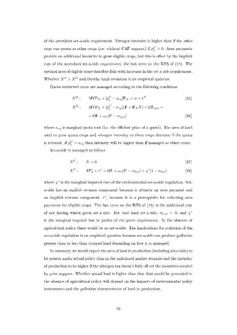
of the attendant set-a-side requirement. Nitrogen intensity is higher than if the other

crop was grown as other crops (i.e. without CAP support) if pCj > 0. Area payments

provide an additional incentive to grow eligible crops, but this is o�set by the implicit

cost of the attendant set-a-side requirement, the last term on the RHS of (14). The

optimal area of eligible crops therefore falls with increases in the set-a-side requirement.

Whether XS > XO and thereby total emissions is an empirical question.

Quota restricted crops are managed according to the following conditions

NQ : MVPN + [pCj − κrq]FN = w + tN (15)

XQ : MVPX + [pCj − κrq](F+ FXX) + ESrjm =

= OL + ωr(θr − σj,m) (16)

where κrq is marginal quota rent (i.e. the e�cient price of a quota). The area of land

used to grow quota crops and nitrogen intensity to these crops decrease if the quota

is reduced. If pCj > κrq then intensity will be higher than if managed as other crops.

Set-a-side is managed as follows

NS : N = 0 (17)

XS : APrk + τ r = OL + ωr(θr − σkm) + χr(1− σkm) (18)

where χr is the marginal imputed cost of the environmental set-a-side regulation. Set-

a-side has an explicit revenue component because it attracts an area payment and

an implicit revenue component, τ r, because it is a prerequisite for collecting area

payments for eligible crops. The last term on the RHS of (18) is the additional cost

of not having winter-green set-a-side. For bare land set-a-side, σk,m = 0, and χr

is the marginal imputed loss in pro�ts of the green requirement. In the absence of

agricultural policy there would be no set-a-side. The implications for pollution of the

set-a-side regulation is an empirical question because set-a-side can produce pollution

greater than or less than cropped land depending on how it is managed.

In summary, we would expect the area of land in production (including set-a-side) to

be greater under actual policy than in the unfettered market scenario and the intensity

of production to be higher if the nitrogen tax doesn't fully o�-set the incentives created

by price support. Whether actual load is higher than that that would be generated in

the absence of agricultural policy will depend on the impacts of environmental policy

instruments and the pollution characteristics of land in production.

10

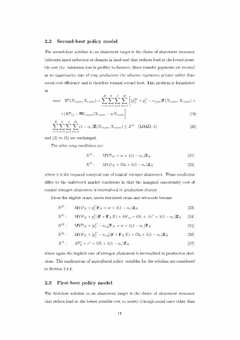
2.2 Second-best policy model

The second-best solution to an abatement target is the choice of abatement measures

(nitrogen input reduction or changes in land-use) that reduces load at the lowest possi-

ble cost (i.e. minimum loss in pro�ts) to farmers. Since transfer payments are treated

as an opportunity cost of crop production the solution represents private rather than

social cost-e�ciency and is therefore termed second-best. This problem is formulated

as

max Π2(Nrsjm, Xrsjm) =R∑

r=1

S∑s=1

J∑j=1

M∑m=1

[(pW

j + pCj − crjm)F(Nrsjm, Xrsjm) +

+(APrj −HCrsjm)Xrsjm − wNrsjm

](19)

R∑r=1

S∑s=1

J∑j=1

M∑m=1

(1− αr)Z(Nrsjm, Xrsjm) ≤ ZA (LOAD, λ) (20)

and (2) to (5) are unchanged.

The other crop conditions are

NO : MVPN = w + λ(1− αr)ZN (21)

XO : MVPX = OL + λ(1− αr)ZX (22)

where λ is the imputed marginal cost of coastal nitrogen abatement. These conditions

di�er to the unfettered market conditions in that the marginal opportunity cost of

coastal nitrogen abatement is internalized in production choices.

Those for eligible crops, quota restricted crops and set-a-side become

NE : MVPN + pCj FN = w + λ(1− αr)ZN (23)

XE : MVPX + pCj (F+ FXX) + APrj = OL + .1τ r + λ(1− αr)ZX (24)

NQ : MVPN + [pCj − κrq]FN = w + λ(1− αr)ZN (25)

XQ : MVPX + [pCj − κrq](F+ FXX) = OL + λ(1− αr)ZX (26)

XS : APrk + τ r = OL + λ(1− αr)ZX (27)

where again the implicit cost of nitrogen abatement is internalized in production deci-

sions. The implications of agricultural policy variables for the solution are considered

in Section 2.4.1.

2.3 First-best policy model

The �rst-best solution to an abatement target is the choice of abatement measures

that reduce load at the lowest possible cost to society (though social costs other than

11

those related to commodity and pollution production are ignored). Income support is

treated as a transfer and not an opportunity cost. This problem is formulated as

max Π1(Nrsjm, Xrsjm) =R∑

r=1

S∑s=1

J∑j=1

M∑m=1

[(pW

j − crjm)F(Nrsjm, Xrsjm) +

+HCrsjmXrsjm − wNrsjm

](28)

and (2), (3) and (20) are unchanged. Under the �rst-best policy there is no set-a-side

and resources are allocated to crop production according to (21) and (22)�it is no

longer necessary to distinguish between eligible and quota crops. These are identical to

the unfettered market conditions with the exception that the implicit cost of nitrogen

abatement is taken into consideration. Thus if ZA is interpreted as the socially optimal

nitrogen load then the solution to the �rst-best problem implies that the social MVP

of nitrogen and MVP of land should be equated with the marginal social cost of using

these resources in crop production. In the next section I study the characteristics of

all three solutions using comparative static analysis.

2.4 Comparative static analysis

Assuming a unique maximum solution exits2 for each of the problems presented above,

then the FOCs de�ne the choice variables as implicit functions of the parameters of

the relevant solution (actual, �rst-best or second-best). Optimal inputs of land and

nitrogen can therefore be expressed as Xjmrs = X(p, c, AP, ES,HC, w, t) for land and

Njmrs = N(p, c, AP, ES,HC,w, t) for nitrogen in generic form. Attendant nitrogen

emissions are thus Zjmrs = Z(Njmrs, Xjmrs) and total pollution load is simply the

sum of pollution from all sources, i.e. all combinations of jmrs, less retention (i.e αr

which is now suppressed) .

Though the model allows for a multitude of land-uses it is su�cient to consider

only two to derive theoretical insights. So lets reduce the land-use choice variables

to X and Y , where X is the area of land in the production of crop x and Y the

area of crop y. Further, assume N is nitrogen input in the production of x and that2This will be the case if the objective function is concave and the constraints form a convex set. By

assumption the yield functions are concave and the load constraint convex. Since the function formed

by the sum of concave and linear functions is itself concave the objective functions must be concave,

and similarly since the sum of convex and linear functions is a convex function the constraints must

form a convex set.

12

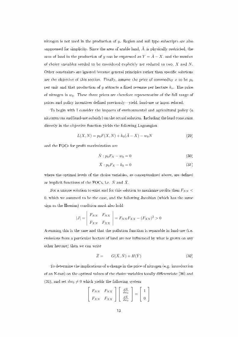
nitrogen is not used in the production of y. Region and soil type subscripts are also

suppressed for simplicity. Since the area of arable land, A, is physically restricted, the

area of land in the production of y can be expressed as Y = A −X, and the number

of choice variables needed to be considered explicitly are reduced to two, X and N .

Other constraints are ignored because general principles rather than speci�c solutions

are the objective of this section. Finally, assume the price of commodity x to be p0

per unit and that production of y attracts a �xed revenue per hectare ko. The price

of nitrogen is w0. These three prices are therefore representative of the full range of

prices and policy incentives de�ned previously�yield, land-use or input related.

To begin with I consider the impacts of environmental and agricultural policy (a

nitrogen tax and land-use subsidy) on the actual solution. Including the land constraint

directly in the objective function yields the following Lagrangian

L(X, N) = p0F (X, N) + k0(A−X)− w0N (29)

and the FOCs for pro�t maximization are

N : p0FN − w0 = 0 (30)

X : p0FX − k0 = 0 (31)

where the optimal levels of the choice variables, as conceptualized above, are de�ned

as implicit functions of the FOCs, i.e. N and X.

For a unique solution to exist and for this solution to maximize pro�ts then FNN <

0, which we assumed to be the case, and the following Jacobian (which has the same

sign as the Hessian) condition must also hold

|J | =

∣∣∣∣∣∣ FNN FNX

FXN FXX

∣∣∣∣∣∣ = FNNFXX − (FXN )2 > 0

Assuming this is the case and that the pollution function is separable in land-use (i.e.

emissions from a particular hectare of land are not in�uenced by what is grown on any

other hectare) then we can write

Z = G(X, N) + H(Y ) (32)

To determine the implications of a change in the price of nitrogen (e.g. introduction

of an N-tax) on the optimal values of the choice variables totally di�erentiate (30) and

(31), and set dw0 6= 0 which yields the following system FNN FNX

FXN FXX

dNdw0

dXdw0

=

1

0

13

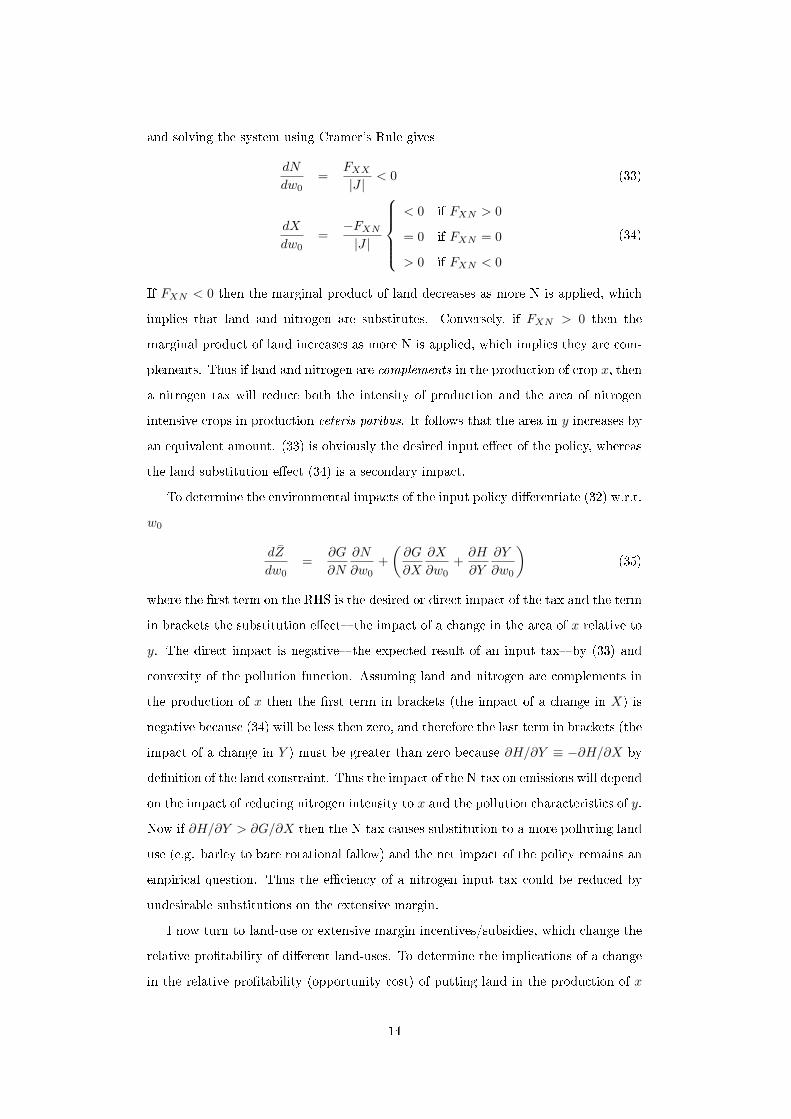
and solving the system using Cramer's Rule gives

dN

dw0=

FXX

|J |< 0 (33)

dX

dw0=

−FXN

|J |

< 0 if FXN > 0

= 0 if FXN = 0

> 0 if FXN < 0

(34)

If FXN < 0 then the marginal product of land decreases as more N is applied, which

implies that land and nitrogen are substitutes. Conversely, if FXN > 0 then the

marginal product of land increases as more N is applied, which implies they are com-

plements. Thus if land and nitrogen are complements in the production of crop x, then

a nitrogen tax will reduce both the intensity of production and the area of nitrogen

intensive crops in production ceteris paribus. It follows that the area in y increases by

an equivalent amount. (33) is obviously the desired input e�ect of the policy, whereas

the land substitution e�ect (34) is a secondary impact.

To determine the environmental impacts of the input policy di�erentiate (32) w.r.t.

w0

dZ

dw0=

∂G

∂N

∂N

∂w0+

(∂G

∂X

∂X

∂w0+

∂H

∂Y

∂Y

∂w0

)(35)

where the �rst term on the RHS is the desired or direct impact of the tax and the term

in brackets the substitution e�ect�the impact of a change in the area of x relative to

y. The direct impact is negative�the expected result of an input tax�by (33) and

convexity of the pollution function. Assuming land and nitrogen are complements in

the production of x then the �rst term in brackets (the impact of a change in X) is

negative because (34) will be less then zero, and therefore the last term in brackets (the

impact of a change in Y ) must be greater than zero because ∂H/∂Y ≡ −∂H/∂X by

de�nition of the land constraint. Thus the impact of the N-tax on emissions will depend

on the impact of reducing nitrogen intensity to x and the pollution characteristics of y.

Now if ∂H/∂Y > ∂G/∂X then the N-tax causes substitution to a more polluting land

use (e.g. barley to bare rotational fallow) and the net impact of the policy remains an

empirical question. Thus the e�ciency of a nitrogen input tax could be reduced by

undesirable substitutions on the extensive margin.

I now turn to land-use or extensive margin incentives/subsidies, which change the

relative pro�tability of di�erent land-uses. To determine the implications of a change

in the relative pro�tability (opportunity cost) of putting land in the production of x

14

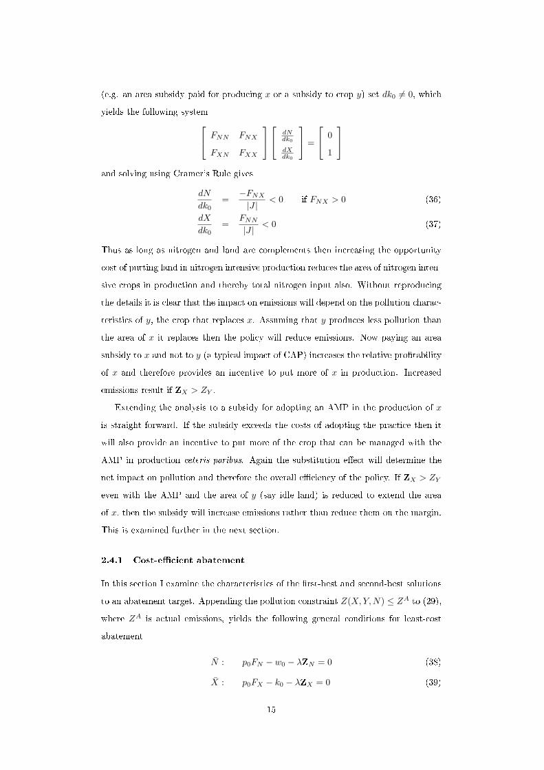
(e.g. an area subsidy paid for producing x or a subsidy to crop y) set dk0 6= 0, which

yields the following system FNN FNX

FXN FXX

dNdk0

dXdk0

=

0

1

and solving using Cramer's Rule gives

dN

dk0=

−FNX

|J |< 0 if FNX > 0 (36)

dX

dk0=

FNN

|J |< 0 (37)

Thus as long as nitrogen and land are complements then increasing the opportunity

cost of putting land in nitrogen intensive production reduces the area of nitrogen inten-

sive crops in production and thereby total nitrogen input also. Without reproducing

the details it is clear that the impact on emissions will depend on the pollution charac-

teristics of y, the crop that replaces x. Assuming that y produces less pollution than

the area of x it replaces then the policy will reduce emissions. Now paying an area

subsidy to x and not to y (a typical impact of CAP) increases the relative pro�tability

of x and therefore provides an incentive to put more of x in production. Increased

emissions result if ZX > ZY .

Extending the analysis to a subsidy for adopting an AMP in the production of x

is straight forward. If the subsidy exceeds the costs of adopting the practice then it

will also provide an incentive to put more of the crop that can be managed with the

AMP in production ceteris paribus. Again the substitution e�ect will determine the

net impact on pollution and therefore the overall e�ciency of the policy. If ZX > ZY

even with the AMP and the area of y (say idle land) is reduced to extend the area

of x, then the subsidy will increase emissions rather than reduce them on the margin.

This is examined further in the next section.

2.4.1 Cost-e�cient abatement

In this section I examine the characteristics of the �rst-best and second-best solutions

to an abatement target. Appending the pollution constraint Z(X, Y,N) ≤ ZA to (29),

where ZA is actual emissions, yields the following general conditions for least-cost

abatement

N : p0FN − w0 − λZN = 0 (38)

X : p0FX − k0 − λZX = 0 (39)

15

λ : ZA − Z(X, Y,N) = 0 (40)

where (40) simply restates the pollution constraint and λ is the shadow price of the

pollution constraint. This implies that in the optimum

p0FN − w0

ZN=

p0FX − k0

ZX=

k0

ZY= λ (41)

which states that reducing pollution at minimum cost (i.e. loss in pro�ts) requires the

marginal loss in pro�t of abating an extra unit of pollution by (marginally) reducing

nitrogen input or the area of x and y should be equal, and in the optimum equal to

λ to achieve cost e�ciency (Baumol, 1972). Which is the familiar equi-marginal cost

principle of cost minimization.

To begin with I determine the impact of a change in the emissions constraint.

Totally di�erentiating (38), (39) and (40) and setting dZA 6= 0 yields the systemA C −ZN

C B −ZX

−ZN −ZX 0

dNdZA

dXdZA

dλdZA

=

0

0

−1

where A = p0FNN − λZNN < 0, B = p0FXX − λZXX < 0 by concavity of the

yield function and convexity of the pollution function, and C = p0FNX − λZNX =

p0FXN − λZXN by Young's theorem and

|J ′| = −AZ2X + CZXZN − ZN (BZN − CZZ) (42)

Assuming |J ′| > 0, which guarantees a unique solution that maximizes pro�ts given

the load constraint, then solving the system using Cramer's Rule gives

dN

dZA=

CZX −BZN

|J ′|≤ 0 (43)

dX

dZA=

CZN −AZX

|J ′|≤ 0 (44)

dλ

dZA=

C2 −AB

|J ′|≤ 0 (45)

Intuitively all three derivatives should be less than or equal to zero, because if

not then pro�ts could not have been maximized before the constraint was tightened.

Observe, if the constraint Z ≤ ZA + ∆ZA could be achieved at higher pro�t than

Z ≤ ZA, then pro�ts could be increased for Z ≤ ZA by reducing emissions. Further,

for (43) and (44) to hold then C < 0 if FNX , ZNX > 0.

To determine the impact of area subsidies (a de�ning di�erence between the �rst

and second best models) and repeating the same procedures but setting dk0 6= 0 yields

dN

dk0=

ZNZX

|J ′|> 0 (46)

16

dX

dk0=

−Z2N

|J ′|< 0 (47)

dλ

dk0=

AZX − CZN

|J ′|(48)

and dλ/dk0 < 0 if |AZX | > |CZN | because C < 0. Thus increasing k0�the relative

pro�tability of y�causes a reduction in the area of X, an increase in nitrogen input

and a reduction in marginal abatement cost. That is it becomes relatively cheaper for

the farmer to change land-use than to reduce nitrogen input ceteris paribus. Similarly,

an area payment to x is equivalent to reducing k0, which implies a greater area of

x and lowered nitrogen input to maintain emissions at ZA. Thus the higher the

�xed income component of total pro�ts per hectare, the less cost-e�cient it will be to

change land-use and the higher the cost-e�cient nitrogen input reduction. We would

therefore expect more land in intensive crop production in the second-best solution, but

farmed less intensively and with AMPs. The elimination of subsidies in the �rst-best

solution reduces the private opportunity cost of switching to less polluting land-uses

such as idling land and increases it for adopting AMPs. Thus we should expect this

solution to be characterized by a greater area of idled land and higher intensity for

land kept in commodity production. Since the least productive land will be taken out

of production �rst this solution implies that intensive commodity production will be

more concentrated and intensively farmed, and less productive land retired or put in

non-intensive uses from a nitrogen control perspective.

In summary, a nitrogen tax reduces intensity ceteris paribus but the impact on

emissions will be conditional on substitution e�ects on the extensive margin. Similarly,

area subsidies for a particular land-use provide an incentive to increase the area of

the subsidized land-use relative to non-subsidized uses. As with an input tax the net

impact on emissions will be conditional on substitution e�ects on the extensive margin.

Signi�cant substitution e�ects could therefore reduce the e�ciency of incentive based

policies. CAP support implies that a second-best solution would maintain a greater

area of land in intensive crop production and abatement goals met with relatively high

reductions in intensity and the adoption of AMPs in intensively famed regions. A �rst

best solution would maintain relatively higher intensity for land in production and

retire relatively more land from production. From a nitrogen pollution perspective the

�rst-best solution is to concentrate intensive crop production and to remove land that

generates low pro�t per unit nitrogen pollution from intensive commodity production.

In contrast the second-best solution is to have widespread and less intensive, and

17

therefore less cost-e�ective commodity production. The signi�cance of the di�erences

between the actual, second-best and �rst-best solutions were addressed in the ensuing

empirical study.

3 Empirical study�background and input data

3.1 Study area

There are approximately 2.3 million hectares of arable land in Southern Sweden of

which 1.5 million hectares are spread only with mineral fertilizers. The sub-artic

region of northern Sweden was omitted from the study because it contributes only

marginally to the Baltic nitrogen problem and to sector pro�ts.

The availability of data has largely dictated the degree of spatial di�erentiation.

The study-area was divided into nine regions that are reasonably homogeneous in

regard to production (i.e. yields, crops and management practices) and climatic con-

ditions, Figure 1. Land is typically covered with grains (55% of total area), grasses

(25%), fallow (10%), oil-seeds (5%), vegetables (2%), sugarbeets (1.5%), salix (1%)

and potatoes (0.5%) (Statistics Sweden, 2000). Sugarbeets and potatoes are by far

the most pro�table crops, however, sugar quotas and suitable land constrain output.

Grasses and salix are the least pro�table outputs, but also produce low emissions.

Figure 1: Map of Sweden and regions

Not included

Table 1 provides an overview of important agricultural and pollution statistics for

each region. In the �rst column, spring barley grown on a medium-clay soil is used as

a representative crop to compare pro�tability (gross-margin, SEK'000/ha) and arable

emissions (e, kg/ha) between regions. Emission rates can be up to 50% higher for a

light-sandy soil and 50% lower for a heavy-clay soil, for any given crop and management

practice. Leaching from permanent fallow/grass can be as low as 4 kg/ha and up to

80 kg/ha for spring rape. Column 2 is regional or gross arable emissions, followed

by average retention, net coastal load, annual precipitation and the distribution of

representative soils�light (l-s), medium (m-c) and heavy (h-c).

Each region (the rows of Table 1) is introduced brie�y: Götaland's southern plains-

18

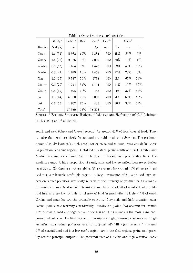
Table 1: Overview of regional statistics

Barleya Leachb Retc Loadd Precb Soilsb

Region GM (e) kg kg mm l-s m-c h-c

Gss-s 1.6 (34) 5 982 10% 5 384 300 45% 55% 0%

Gss-w 1.6 (36) 2 136 5% 2 030 400 82% 16% 1%

Gmb-s 0.9 (33) 1 524 5% 1 448 300 32% 43% 25%

Gmb-e 0.9 (21) 1 619 10% 1 458 200 27% 73% 0%

Gns 1.2 (25) 5 587 50% 2794 300 2% 65% 33%

Gsk-w 0.5 (29) 1 714 35% 1 114 400 11% 49% 39%

Gsk-e 0.5 (17) 925 50% 463 200 4% 32% 64%

Ss 1.1 (24) 6 160 50% 3 080 200 4% 66% 30%

Ssk 0.6 (33) 1 932 75% 483 300 16% 30% 54%

Total 27 580 34% 18 254Sources: a Regional Enterprize Budgets, b Johnsson and Ho�mann (1997), c Arheimer

et al. (1997) and d modelled.

south and west (Gss-s and Gss-w) account for around 41% of total coastal load. They

are also the most intensively farmed and pro�table regions in Sweden. The predomi-

nance of sandy-loam soils, high precipitation rates and minimal retention de�ne these

as pollution sensitive regions. Götaland's eastern plains-south and east (Gmb-s and

Gmb-e) account for around 16% of the load. Intensity and pro�tability lie in the

medium range. A high proportion of sandy soils and low retention increase pollution

sensitivity. Götaland's northern plains (Gns) account for around 15% of coastal load

and it is a relatively pro�table region. A large proportion of h-c soils and high re-

tention reduce pollution sensitivity relative to the intensity of production. Götaland's

hills-west and east (Gsk-w and Gsk-e) account for around 8% of coastal load. Pro�ts

and intensity are low, but the total area of land in production is high�15% of total.

Grains and grass-ley are the principle outputs. Clay soils and high retention rates

reduce pollution sensitivity considerably. Svealand's plains (Ss) account for around

17% of coastal load and together with the Gss and Gns regions is the most signi�cant

region output wise. Pro�tability and intensity are high, however, clay soils and high

retention rates reduce pollution sensitivity. Svealand's hills (Ssk) account for around

3% of coastal load and is a low pro�t region. As in the Gsk regions grains and grass-

ley are the principle outputs. The predominance of h-c soils and high retention rates

19

greatly reduce pollution risk.

The principle abatement strategy available to farmers is to minimize concentrations

of mineral nitrogen in soils over the Swedish autumn and winter. This can be achieved

by reducing fertilization rates (ceteris paribus), adopting less polluting management

practices (spring-tillage or catch-crop system) or substituting to less polluting land-

uses (grains to grass or energy, or taking land out of production).

3.2 Agricultural production

Crop enterprize budgets prepared by agricultural extension services by region were uti-

lized to determine yield and hectare dependent costs, i.e. crjm and HCrsjm, (Regional

Enterprize Budgets). Crop prices and agricultural policy payments were taken from

o�cial statistics. Field and farm sizes used by extension services to estimate �xed

costs were assumed to be representative of crop farms in each region. These building

blocks were then used to create a representative farm for each region.

Standard quadratic yield functions (estimated using experimental data) were used

for determining yield responses to changes in nitrogen intensity. The functions were

however calibrated for regional variations in crop productivity. In the calibration

procedure (Appendix A), regional average crop yields and nitrogen application rates

from published statistics were used as proxies for pro�t maximizing input and output

levels. A similar approach is used by Fleming and Adams (1997).

This information and relevant production constraints, however, is not su�cient to

explain observed activity levels. To calibrate the model to observed activity levels in

the base year (1999) a procedure utilizing Positive Mathematical Programming (PMP)

(Howitt, 1995) was implemented (Appendix B).

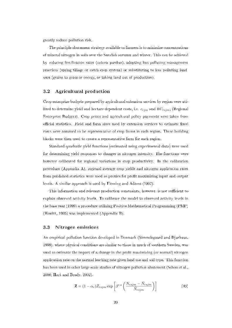
3.3 Nitrogen emissions

An empirical pollution function developed in Denmark (Simmelsgaard and Djurhuus,

1998), where physical conditions are similar to those in much of southern Sweden, was

used to estimate the impact of a change in the pro�t maximizing (or normal) nitrogen

application rate on the normal leaching rate given land use and soil type. This function

has been used in other large scale studies of nitrogen pollution abatement (Schou et al.,

2000; Hart and Brady, 2002).

Z = (1− αr)Zrsjm exp[βr,s

(Nrsjm − Nrsjm

Nrsjm

)](49)

20

where Zrsjm is the average or normal rate of leaching (kg/ha) and Nrsjm is the normal

nitrogen intensity. βr,s is a fertilization coe�cient which relates a proportional change

in the normal nitrogen dose to the concomitant change in leaching.

Leaching data were generated in simulation studies conducted with the soil-nitrogen

model SOIL-N (Johnsson et al., 1987). SOIL-N is a one-dimensional model that sim-

ulates the movement and transportation of nitrate-nitrogen through arable soils (Ni-

trate transported below the root zone and therefore unavailable to plants is de�ned as

leached nitrogen). Data was available for the 9 production-climate regions described

above, 10 crop types (barley/oates, spring and autumn wheat, rye, sugarbeets, pota-

toes, annual and multi-year grass ley or energy, and spring and autumn oilseed), 3

representative soil types (l-s, m-c and h-c) (Johnsson and Ho�mann, 1997) and 3 al-

ternative management practices (catch crop, spring tillage or catch crop followed by

spring tillage) (Ho�mann et al., 1999).

Mean nitrogen transport or retention coe�cients, αr, were calculated for each re-

gion from data produced in studies using the HBV-N riverine nitrogen transport model

(Arheimer et al., 1997). The model estimates retention of leached nitrate-nitrogen dur-

ing transport via surface waters to the coastline (i.e. potential groundwater transports

are ignored).

4 Results

The empirical model can be classi�ed as a large scale, nonconvex, and nonlinear pro-

gramming model. It was solved in GAMS using the CONOPT2 solver which is well

suited to problems that are highly nonlinear but smooth in the constraints such as this.

Nonconvexity, a result of the possibility to switch between land-uses, implies that a

solution wont necessarily be a global solution. An abatement target was achieved step-

wise by incrementing abatement through 2% intervals between solutions and using the

current solution as initial or starting values for the subsequent problem and so on. The

'globalness' of a solution was investigated through scenario analysis, i.e. by reducing

the ranges of selected choice variables (e.g. nitrogen reductions were limited to 10%

of the normal rate, all land was required to be in production, etc). But none of these

scenarios achieved the targets at lower cost. With these di�culties in mind I now

present the results of the study.

Actual Swedish nitrogen abatement incentives comprise a national or single-rate

21

nitrogen fertilizer tax (SEK1.80/kg N which is roughly 30% of the price of nitrogen),

and single-rate subsidies in the Gss, Gmb, and Gns regions for a catch/cover crop

(SEK900/ha) and adoption of spring-tillage practices (SEK400/ha). These measures

can also be combined (SEK1300/ha). Initially a linear program was solved to calibrate

the model (Section 3.2) to observed activity levels in the base year (1999) and to check

the integrity of input data. Actual nitrogen abatement instruments were subsequently

removed from the calibrated nonlinear program to generate a baseline solution. The

actual policy solution produced 21% abatement compared to the baseline. Using 21%

as the abatement target the second and �rst best solutions were then generated. The

solutions are summarized in Table 2. Maximized pro�ts under the �rst-best solution

generated 38% less pollution than the baseline so the pollution constraint was not

active in this solution. Nitrogen policy is simply correcting for the additional pollution

generated by agricultural policy. Baseline pro�t was SEK249/kg N load which can be

used to put average abatement costs (Cost-e�eciency ratio) in some perspective. As

expected actual abatement costs exceed both benchmarks. The sources of ine�ciency

are explored below.

Table 2: Solution summaries for 21% abatementBase Actual Second First

Pro�t (SEK million) 4,682 4,509 4,656 4,163*

Load (tonnes) 18,182 14,316 14,316 11,245

Abatement Cost (SEK million) 173 26 n/a

Cost-e�eciency ratio (SEK/kg N) 45.22 7.36 n/a* CAP income is maintained at Baseline level by a lump-sum transfer but yield related losses

are not compensated.

Table 3 shows how the allocation of relative abatement varied between regions

and solutions. Actual policy caused excessive abatement in the Gss and Gmb regions

compared with the second-best solution. But this result is relative to the modelled

target, 21%. Comparing the second-best solution with the �rst-best solution for a 50%

target (the actual policy goal!) shows that the second-best solution weights abatement

to the most pro�table agricultural region, Gss and the least Ssk. Considering this table

as a whole implies that increasing relative abatement in the Gmb, Gns, Gsk and Ss

regions would increase overall abatement e�ciency if the target is 50% total abatement.

These results follow from the theoretical insight that a second-best solution keeps a

greater area of land in intensive commodity production that is farmed relatively less

22

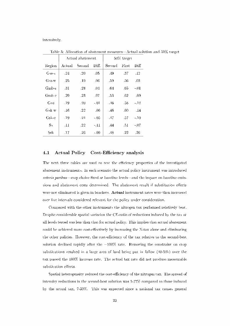
intensively.

Table 3: Allocation of abatement measures�Actual solution and 50% target

Actual abatement 50% target

Region Actual Second Di�. Second First Di�

Gss-s .24 .20 .05 .49 .37 .12

Gss-w .25 .19 .06 .59 .56 .03

Gmb-s .31 .28 .04 .64 .65 -.01

Gmb-e .29 .23 .07 .53 .62 -.09

Gns .19 .20 -.01 .46 .58 -.12

Gsk-w .16 .22 -.06 .46 .60 -.14

Gsk-e .19 .24 -.05 .47 .57 -.10

Ss .11 .22 -.11 .44 .51 -.07

Ssk .17 .26 -.09 .48 .22 .26

4.1 Actual Policy�Cost-E�ciency analysis

The next three tables are used to test the e�ciency properties of the investigated

abatement instruments. In each scenario the actual policy instrument was introduced

ceteris paribus�crop choice �xed at baseline levels�and the impact on baseline emis-

sions and abatement costs determined. The abatement result if substitution e�ects

were not eliminated is given in brackets. Actual instrument rates were then increased

over �ve intervals considered relevant for the policy under consideration.

Compared with the other instruments the nitrogen tax performed relatively best.

Despite considerable spatial variation the CE-ratio of reductions induced by the tax at

all levels tested was less than that for actual policy. This implies that actual abatement

could be achieved more cost-e�ectively by increasing the N-tax alone and eliminating

the other policies. However, the cost-e�ciency of the tax relative to the second-best

solution declined rapidly after the +100% rate. Removing the constraint on crop

substitutions resulted in a large area of land being put in fallow (40-52k) once the

tax passed the 100% increase-rate. The actual tax rate did not produce measurable

substitution e�ects.

Spatial heterogeneity reduced the cost-e�ciency of the nitrogen tax. The spread of

intensity reductions in the second-best solution was 1-77% compared to those induced

by the actual tax, 7-33%. This was expected since a national tax causes general

23

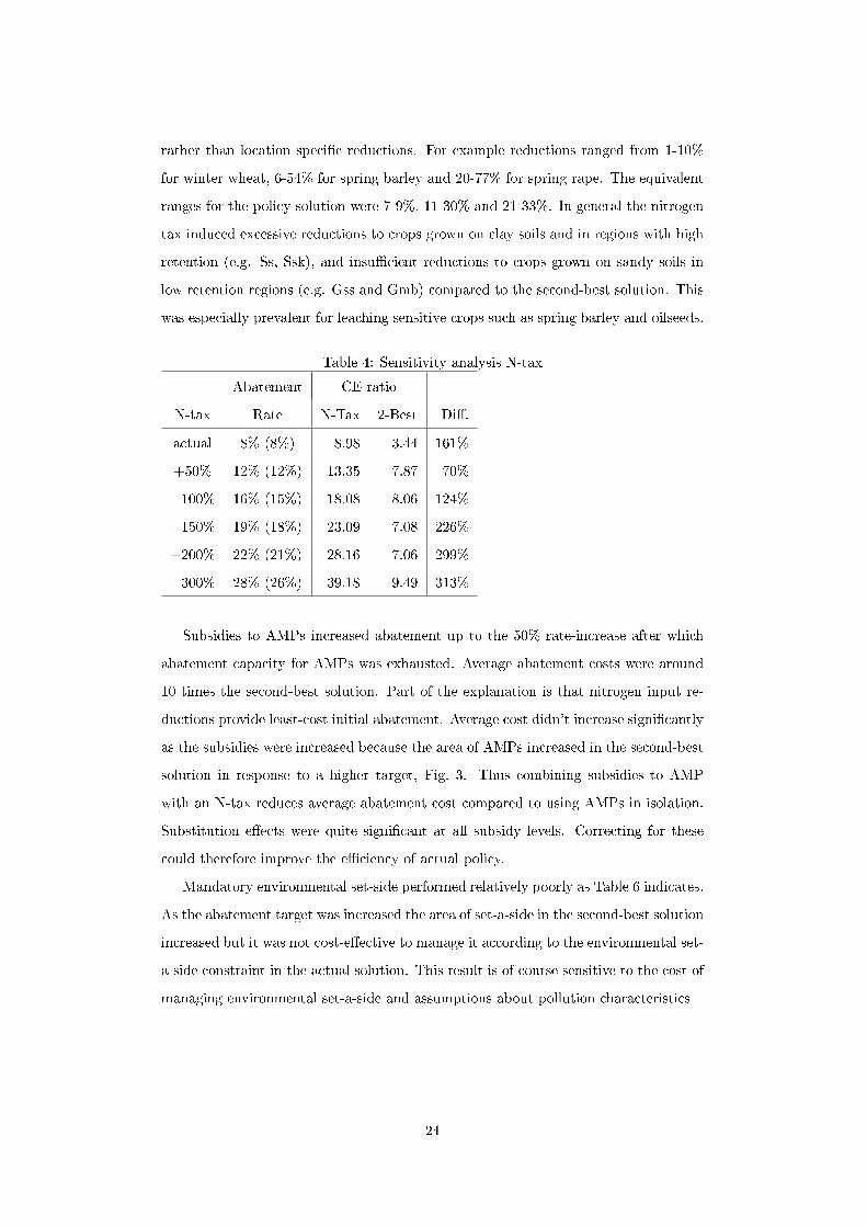
rather than location speci�c reductions. For example reductions ranged from 1-10%

for winter wheat, 6-54% for spring barley and 20-77% for spring rape. The equivalent

ranges for the policy solution were 7-9%, 11-30% and 21-33%. In general the nitrogen

tax induced excessive reductions to crops grown on clay soils and in regions with high

retention (e.g. Ss, Ssk), and insu�cient reductions to crops grown on sandy soils in

low retention regions (e.g. Gss and Gmb) compared to the second-best solution. This

was especially prevalent for leaching sensitive crops such as spring barley and oilseeds.

Table 4: Sensitivity analysis N-tax

Abatement CE-ratio

N-tax Rate N-Tax 2-Best Di�.

actual 8% (8%) 8.98 3.44 161%

+50% 12% (12%) 13.35 7.87 70%

+100% 16% (15%) 18.08 8.06 124%

+150% 19% (18%) 23.09 7.08 226%

+200% 22% (21%) 28.16 7.06 299%

+300% 28% (26%) 39.18 9.49 313%

Subsidies to AMPs increased abatement up to the 50% rate-increase after which

abatement capacity for AMPs was exhausted. Average abatement costs were around

10 times the second-best solution. Part of the explanation is that nitrogen input re-

ductions provide least-cost initial abatement. Average cost didn't increase signi�cantly

as the subsidies were increased because the area of AMPs increased in the second-best

solution in response to a higher target, Fig. 3. Thus combining subsidies to AMP

with an N-tax reduces average abatement cost compared to using AMPs in isolation.

Substitution e�ects were quite signi�cant at all subsidy levels. Correcting for these

could therefore improve the e�ciency of actual policy.

Mandatory environmental set-side performed relatively poorly as Table 6 indicates.

As the abatement target was increased the area of set-a-side in the second-best solution

increased but it was not cost-e�ective to manage it according to the environmental set-

a-side constraint in the actual solution. This result is of course sensitive to the cost of

managing environmental set-a-side and assumptions about pollution characteristics

24

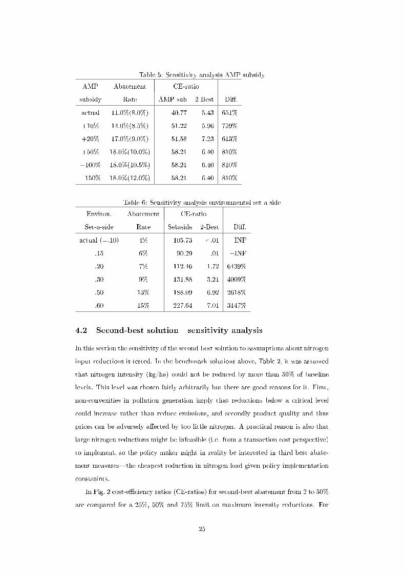
Table 5: Sensitivity analysis AMP subsidy

AMP Abatement CE-ratio

subsidy Rate AMP-sub 2-Best Di�.

actual 11.0%(8.0%) 40.77 5.43 651%

+10% 14.0%(8.5%) 51.22 5.96 759%

+20% 17.0%(9.0%) 51.58 7.23 613%

+50% 18.0%(10.0%) 58.21 6.40 810%

+100% 18.0%(10.5%) 58.21 6.40 810%

+150% 18.0%(12.0%) 58.21 6.40 810%

Table 6: Sensitivity analysis environmental set-a-side

Environ. Abatement CE-ratio

Set-a-side Rate Setaside 2-Best Di�.

actual (=.10) 4% 105.73 <.01 +INF

.15 6% 90.29 .01 +INF

.20 7% 112.46 1.72 6439%

.30 9% 131.88 3.21 4009%

.50 13% 188.09 6.92 2618%

.60 15% 227.64 7.01 3147%

4.2 Second-best solution�sensitivity analysis

In this section the sensitivity of the second-best solution to assumptions about nitrogen

input reductions is tested. In the benchmark solutions above, Table 2, it was assumed

that nitrogen intensity (kg/ha) could not be reduced by more than 50% of baseline

levels. This level was chosen fairly arbitrarily but there are good reasons for it. First,

non-convexities in pollution generation imply that reductions below a critical level

could increase rather than reduce emissions, and secondly product quality and thus

prices can be adversely a�ected by too little nitrogen. A practical reason is also that

large nitrogen reductions might be infeasible (i.e. from a transaction cost perspective)

to implement, so the policy maker might in reality be interested in third best abate-

ment measures�the cheapest reduction in nitrogen load given policy implementation

constraints.

In Fig. 2 cost-e�ciency ratios (CE-ratios) for second-best abatement from 2 to 50%

are compared for a 25%, 50% and 75% limit on maximum intensity reductions. For

25

the benchmark solution, 21%, there is little di�erence between the CE-ratios, however

at the 50% level the di�erence in total cost between the 75% and 25% scenarios is

SEK86 million. Nitrogen reduction limitations could therefore have important policy

implications for achieving greater abatement.

Figure 2: Second-best abatement costs�sensitivity to constraint on nitrogen input

reductions

See attachment

The impact of nitrogen reduction limitations for choice of AMPs is shown in Fig. 3,

which shows the expansion of AMPs for each assumption with increasing abatement.

After the 18% level the assumption has a signi�cant impact on the adoption of AMPs.

Thus in the absence of nitrogen reductions alternative management practices represent

an important alternative measure.

Figure 3: Alternative management practices�sensitivity to constraint on nitrogen

reductions

See attachment

The implications of nitrogen reduction limitations for set-a-side was marginal for all

three assumptions�AMPs were more cost-e�ective. Further, environmental set-a-side

did not enter the second-best solution for abatement targets up to 50% and the area

of energy declined as the target was tightened and for all nitrogen reduction levels.

The di�erences in absolute terms were marginal for all assumptions about nitrogen

reductions. On the other hand the area of uncontrolled set-a-side remained fairly

constant up until the 30% level and then increased fairly linearly from around 145k

ha to 230k ha for 50% abatement and a 25% limit on N reductions and 210k ha for

a 75% limit. That the area of land put in set-a-side increased rather than taking it

permanently out of production is due to the area subsidy for set-a-side.

The de�nition of set-a-side used in this study was rotational set-a-side. The dif-

ference being that taking land 'permanently' out of intensive crop production (> 5

years) reduces leaching more signi�cantly. If all fallow could be guaranteed to be kept

out of production permanently and still attract an area subsidy, then abatement costs

26

would be lower than those determined in the second-best solution and the relative cost-

e�ciency of AMPS would decline. This is illustrated further in the �rst-best solution

to a 50% target.

4.3 First-best solution�insights

The �rst-best response to a 50% abatement target was to reduce the area of land in

production, and the results were not particularly sensitive to fertilizer reductions since

it was optimal to maintain relatively high intensity for land in production. Similarly,

alternative management practices did not enter the �rst-best solution. The area of

land in production at the 50% abatement level (and 50% nitrogen limit) was 360k

hectares less than the baseline solution. This corresponds to an area of approximately

130k over and above set-a-side being taken out of commodity production compared

to the second-best solution. In addition, almost 140k hectares were managed with

AMPs in the second-best solution compared to the baseline. Thus the di�erence

between the �rst-best and second-best solutions as predicted in the theoretical section

is how an area of 360k hectares of less productive land should be managed and higher

nitrogen intensity for land left in production. Of this area, a third is currently managed

as set-a-side of which the pollution properties are also fairly uncertain. Conversion

to permanent fallow would not conceivably have great practical signi�cance from a

production point of view but could be important from a pollution perspective.

5 Discussion and Conclusions

Coastal nitrogen abatement is a complex economic problem because spatial variation

or heterogeneity in physical parameters (climate, soils, water transport paths, etc.)

implies that the environmental impact (reduction in coastal load) of a leaching reduc-

tion measure will be location speci�c. In a large catchment, such as the Swedish Baltic

Sea catchment, agricultural production conditions, pro�tability and hence the costs of

changing the production technology to reduce leaching (i.e. abatement measures) also

vary considerably. To achieve cost-e�ective coastal nitrogen abatement the marginal

cost of reducing load needs to be equalized across all pollution sources, in this case

units of arable land (Baumol, 1972).

The costs of collecting the information necessary for ensuring cost-e�ective non-

point source pollution abatement (e.g. arable nitrogen) are generally prohibitive.

27

Rather policies need to be designed to in�uence variables observable at reasonable cost

such as purchased inputs or land management practices. Sweden has implemented a

comprehensive scheme of nitrogen abatement instruments that include a nitrogen tax,

crop management subsidies and land-use regulations. The purpose of this study was to

analyze the economic properties of the Swedish (actual) system. Though it could not

possibly be cost-e�cient it could still have 'better' or 'worse' economic properties�

relative cost-e�ciency, appropriateness of incentives to farmers, etc.�given the imple-

mentation constraints faced by policy makers and the ambitiousness of the abatement

target.

The empirical study was restricted to the chemical fertilizer system in southern Swe-

den. Due to the expanse and heterogeneity of the study-area a spatially distributed

mathematical programming model that linked changes in agricultural production tech-

nologies to coastal nitrogen load was developed. The model was calibrated to observed

production activity levels in 1999 using Positive Mathematical Programming. The

economic properties of the actual policy solution were evaluated by comparing it with

second-best (agricultural policy variables taken as given) and �rst-best (re�ecting so-

cial opportunity costs) solutions. The implications for increasing the current level of

abatement were also considered.

A number of generalizations can be drawn from the theoretical analysis. A nitro-

gen tax should reduce intensity ceteris paribus but the impact on pollution will be

conditional on substitution e�ects on the extensive margin. Similarly, area subsidies

for a particular land-use or land management practice (AMP) provide an incentive to

increase the area of the subsidized land-use relative to non-subsidized uses. The posi-

tive impact of an AMP could therefore be reduced by inappropriate substitutions on

the extensive margin. Agricultural policy (CAP) implies that a second-best solution

(vis-á-vis �rst-best) would maintain a greater and sparser area of land in intensive

crop production. Second-best abatement would therefore require relatively higher re-

ductions in nitrogen intensity and the introduction of pollution reducing management

practices (catch cropping and spring tillage). In comparison, a �rst-best solution would

require land kept in production to be farmed relatively more intensively and thus prof-

itably, and for more marginal land to be taken out of intensive crop production. Thus

a �rst-best solution implies concentration of intensive crop production to a smaller

area of land which should be farmed more e�ectively, whilst a second-best solution im-

plies sparser production and therefore less cost-e�ective commodity production. The

28

choice of e�ciency criterion could therefore be important for determining appropriate

abatement measures and policy instruments.

The principle conclusions of this study are that 1) the Swedish nitrogen tax has

relatively good economic properties 2) subsidies to AMP are only second-best policies

3) undesirable substitution e�ects induced by subsidies to AMP were signi�cant 4)

permanently retiring land from intensive crop production is a �rst-best measure where

as environmental EU set-a-side only a second-best and 5) the choice of e�ciency bench-

mark had important implications for the 'e�cient' allocation of abatement resources

between regions.

The use of single-rate incentives rather than spatially di�erentiated incentives were

an obvious source of cost-ine�ciency but this is well recognized in the literature

(Siebert, 1985). Though not solving the nitrogen problem the Swedish nitrogen tax

was shown to induce relatively cheap abatement gains and provide farmers with an ap-

propriate economic signal. It induces global nitrogen intensity reductions, which were

shown to be �rst-best measures, and provides a reward for continual improvements

in nitrogen e�ciency in crop production. Nor did it induce signi�cant substitution

e�ects at the actual level. There is a substantial debate about the economic merits of

commercial nitrogen taxation, which makes Sweden as the only implementer of such a

policy an interesting case study. Other studies have shown that a unitary tax need not

be overly cost-ine�cient (Helfand and House, 1995; Larson et al., 1996; Brännlund and

Gren, 1999) but these studies concentrate on fairly homogeneous production systems or

highly aggregated data, and therefore consider only a limited amount of heterogeneity.

Highly targeted, information intensive strategies can outperform global policies by a

substantial margin (Babcock et al., 1997; Fleming and Adams, 1997; Carpentier et al.,

1998)�as is also indicated in this study�but these studies ignore transaction costs.

The question thus seems to be whether unitary instruments achieve a desired result

at acceptable cost rather than least-cost. For want of evidence of better alternatives

this seems to be the case for the Swedish nitrogen tax.

Subsidies to catch crops and spring tillage (so called AMPs) were shown to have

less favourable economic properties. Firstly, AMPs were only second-best abatement

measures (i.e. they did not enter the �rst-best solution). Secondly, they caused signif-

icant substitution e�ects by providing an incentive to increase the area of spring sown

crops and to reduce the area of set-a-side (in regions where the set-a-side constraint

was not binding) which reduced cost-e�ciency. Such secondary substitution e�ects of

29

single incentive policies are well documented in the literature (e.g. Bouzaher et al.,

1992, 1995), however, adopting a multiple incentive approach to reduce such e�ects is

less apparent (Bullock and Salhofer, 1998).

Fallow, idle, set-a-side or retired land refers to land kept more or less temporarily

out of commodity production. The de�ning feature of this land-use is that the land

is not in immediate commodity production, however, the way it is managed can vary

considerably which itself can have important implications for pollution levels (Meissner

et al., 1998). Before Sweden joined the EU, fallow was fairly rare and therefore its

pollution properties have been somewhat neglected. In this study if fallow land was

covered permanently with grass (> 5 years without tillage) then it was assumed to

produce only minimal or background leaching, and if included in shorter crop rotations

then levels below or above that for spring-barley depending on the way it was managed.

Today, EU set-a-side represents over 10% of all arable land that is technically in

production and increasing it in response to an increasing abatement target was a

second-best abatement measure. Assumptions about the way it was managed and

the costs thereof are therefore an important caveat on the results. For example if all

set-a-side in the second-best solution was treated as permanent fallow then abatement

costs would fall and the cost-e�cient area of pollution reducing management practices

would decline. Careful consideration must therefore be given to the policy makers

ability to control the management of fallow/set-a-side.

The choice of e�ciency benchmark was important for the determination of relative

abatement between regions. Using the second-best bench-mark abatement was more

concentrated to intensively farmed coastal regions because area payments increased

the relative cost of changing land use in less productive regions. However, when using

the �rst-best bench-mark, yield e�ects were a relatively more important determinant of

abatement costs and resulted in a redistribution of relative abatement e�ort away from

more intensive (pro�table) regions. Relative abatement should be increased in inland

regions to improve the cost-e�ciency of an increasing abatement target according to

both the second and �rst-best solutions.

On a broader note the o�cial abatement target (50%) is far greater than that

achieved by actual policy (21%). Increasing abatement without causing excessive

increases in cost ine�ciencies will require, from the insights of this study, incentives

that also steer land allocation (crop choice) decisions. Further, e�cient land allocation

incentives were not particularly sensitive to soil type. Thus di�erentiating by crop and

30

region (as the present system of area payments is) could be su�cient to produce

relatively low cost abatement.

A discussion on the merits of extensive margin incentives would, however, be amiss

without consideration of area payments. As shown these payments create a signi�cant

restriction on potential low cost abatement measures by preserving status quo land

allocations à la second-best measures. It is frequently argued though, that transfers to

farmers should be interpreted as compensation for the provision of public goods (e.g.

Johnsen, 1993, p.413) and, therefore should (presumably) be included as opportunity

costs of abatement. This argument is, however, increasingly di�cult to defend given

the trade distortions and environmental damage attributable to the current agricul-

tural policy framework in the EU, the CAP (Ingersent et al., 1998; Swinbank, 1999;

Stoate et al., 2001). Coordination of nitrogen and agricultural policy could therefore

yield considerable e�ciency gains from a broader economic perspective.

6 Acknowledgements

I thank Ing-Marie Gren for reading and o�ering valuable comments on various versions

of the manuscript, Markus Ho�mann (previously at Dept. of Soil Sciences, SLU) for

help with nitrogen leaching data and Rob Hart for helpful comments.

31

References

B. Albertsson, M. Kvist, and J. Löfgren. Sector objectives and abatement program

for reducing nutrient losses from agriculture, volume 2000:1. Swedish Board of

Agriculture, Jönköping, 1999. (in Swedish).

B. Arheimer, M. Brandt, G. Grahn, E. Roos, and A. Sjöö. Modelled nitrogen transport,

retention and source apportionment for southern sweden (In Swedish). Technical

report, SMHI Reports Hydrology, Norrköpping, 1997.

B. A. Babcock, J. W. Lakshminarayan, and D. Zilberman. Targeting tools for the

purchase of environmental amenities. Land Economics, 73:325�339, 1997.

W. J. Baumol. On taxation and the control of externalities. American Economic

Review, 62:307�322, 1972.

A. Bouzaher, R. Cabe, A. Carriquiry, and J. F. Shogren. E�ects of environmental

policy on trade-o�s in agri-chemical management. Journal of Environmental Man-

agement, 36:69�80, 1992.

A. Bouzaher, R. Cabe, S. R. Johnson, A. Manale, and J. F. Shogren. Ceepes: An

evolving system for agroenvironmental policy. In J. W. Milon and J. F. Shogren,

editors, Integrating economic and ecological indicators, pages 67�90. Praeger Pub-

lishers, London, 1995.

J. B. Braden, G. V. Johnson, A. Bouzaher, and D. Miltz. Optimal spacial management

of agricultural pollution. American Journal of Agricultural Economics, 71:404�413,

1989.

J. B. Braden and K. Segerson. Information problems in the design of nonpoint-source

pollution policy. In C. S. Russell and J. F. Shogren, editors, Theory, modeling

and experience in the management of nonpoint-source pollution, pages 1�36. Kluwer

Academic Publishers, Boston, 1993.

M. Brady. Imperfect manure and commercial fertilizer substitutability�implications

for environmental policy. (Unpublished) Working Paper, Dept. of Economics, SLU

Box 7013, Sweden, 2002a.

M. Brady. Propagation of uncertainty and the e�ciency of stochastic water pollution

control. (Unpublished) Working Paper, Dept. of Economics, SLU Box 7013, Sweden,

2002b.

32

R. Brännlund and I.-M. Gren. Costs of uniform and di�erentiated charges on a

polluting input: an application to nitrogen fertilizers in sweden. In M. Boman,

R. Brännlund, and B. Kriström, editors, Topics in environmental economics, pages

33�49. Kluwer, Dordrecht, 1999.

D. S. Bullock and K. Salhofer. Measuring the social costs of suboptimal combinations

of policy instruments: General framework and an example. Agricultural Economics,

18:249�259, 1998.

C. L. Carpentier, D. J. Bosch, and S. S. Batie. Using spatial information to reduce

costs of controlling agricultural nonpoint source pollution. Agricultural and Resource

Economics Review, 27:72�84, 1998.

E. Feinerman and E. K. Choi. Second best taxes and quotas in nitrogen regulation.

Natural Resource Modeling, 7:57�84, 1993.

R. A. Fleming and R. M. Adams. The importance of site-speci�c information in the

design of policies to control pollution. Journal of Environmental Economics and

Management, 33:347�358, 1997.

I.-M. Gren. Nutrient reductions to the baltic sea: Ecology, costs and bene�ts. Journal

of Environmental Management, 51:123�143, 1997.

R. C. Gri�n and D. W. Bromley. Agricultural runo� as a nonpoint externality: The-

oretical development. American Journal of Agricultural Economics, 64:547�552,

1982.

R. Hart and M. Brady. Nitrogen in the Baltic Sea�policy implications of stock e�ects.

Journal of Environmental Management, In Press:1�27, 2002.

G. E. Helfand and B. W. House. Regulating nonpoint source pollution under het-

erogeneous conditions. American Journal of Agricultural Economics, 77:1024�1032,

1995.

M. Ho�mann, H. Aronsson, P. Aronsson, H. Nilsson, and B. Albertsson. The farm

model: An empirical nitrogen leaching model. Technical report, Division of Water

Quality Management, SLU., Uppsala, 1999.

R. D. Horan and M. O. Ribaudo. Policy objectives and economic incentives for con-

trolling agricultural sources of pollution. Journal of the American Water Resources

Association, 35:1023�1035, 1999.

33

R. E. Howitt. Positive mathematical programming. American Journal of Agricultural

Economics, 77:329�342, 1995.

W.-Y. Huang and M. LeBlanc. Market-based incentives for addressing, non-point

water quality problems: Residual nitrogen tax approach. Review of Agricultural

Economics, 16:427�440, 1994.

W.-Y. Huang and N. D. Uri. An assessment of alternative agricultural policies to

reduce nitrogen fertilizer use. Ecological Economics, 5:213�234, 1992.

K. A. Ingersent, A. J. Rayner, and R. C. Hine. The reform of the common agricultural

policy: Postscript. In K. A. . R. Ingersent, A.-J.; Hine, editor, The reform of the

Common Agricultural Policy, pages 189�199. Macmillan Press, New York, 1998.

F. H. Johnsen. Economic analyses of measures to control phosphorus run-o� from non-

point agricultural sources. European Review of Agricultural Economics, 20:399�418,

1993.

H. Johnsson, L. Bergström, P. E. Jansson, and K. Paustian. Simulated nitrogen dy-

namics and losses in a layered agricultural soil. Agriculture, Ecosystems and Envi-

ronment, 18:333�356, 1987.

H. Johnsson and M. Ho�mann. Nitrogen leaching from Swedish arable land - calculation

of normal leaching and possible abatement measures (In Swedish). Report 4741,

Swedish EPA, Stockholm, 1997.

R. E. Just and J. M. Antle. Interactions between agricultural and environmental

policies: Conceptual framework. American Economic Review, 80:197�202, 1990.

D. M. Larson, G. E. Helfand, and B. W. House. Second-best tax policies to reduce

nonpoint source pollution. American Journal of Agricultural Economics, 78:1108�

1117, 1996.

R. Meissner, J. Seeger, and H. Rupp. Lysimeter studies in east germany concerning

the in�uence of set aside of intensively fanned land on the seepage water quality.

Agriculture Ecosystems and Environment, 67(2-3):161�173, FEB 1998.

J. R. O'Callaghan. Land use - The interaction of economics, ecology and hydrology.

Chapman and Hall, London, 1996.

34

J. S. Schou, E. Skop, and J. D. Jensen. Integrated agri-environmental modelling: cost-

e�ectiveness analysis of two nitrogen tax instruments in the vejle fjord watershed,

denmark. Journal of Environmental Management, 58:199�212, 2000.

J. F. Shogren. Reforming nonpoint pollution policy. In C. S. Russell and J. F. Shogren,

editors, Theory, modeling and experience in the management of nonpoint-source

pollution, pages 329�345. Kluwer Academic Publishers, Boston, 1993.

J. S. Shortle and J. W. Dunn. The relative e�ciency of agricultural source water

pollution contro l policies. American Journal of Agricultural Economics, 68:668�

677, 1986.

R. C. Shumway and A. A. Chang. Linear programming versus positively estimated

supply functions: An empirical and methodological critique. American Journal of

Agricultural Economics, 59(2):344�57, May 1977.

H. Siebert. Spatial aspects of environmental economics. In A. V. Kneese and J. L.

Sweeney, editors, Handbook of Natural Resource and Energy Economics, pages 125�

164. Elsevier, Amsterdam, 1985.

S. E. Simmelsgaard and J. Djurhuus. An empirical model for estimating nitrate leach-

ing as a�ected by crop type and the long-term fertilizer rate. Soil Use and Manage-

ment, 14:37�43, 1998.

SNV. Nitrogen from land to sea (In Swedish). Report 4735, Swedish EPA, Stockholm,

1997.

C. Stoate, N. Boatman, R. Borralho, C. R. Carvalho, G. de Snoo, and P. Eden.

Ecological impacts of arable intensi�cation in europe. Journal of Environmental

Management, 63(4):337�365, DEC 2001.

A. Swinbank. Cap reform and the wto: Compatibility and developments. European

Review of Agricultural Economics, 26:389�407, 1999.

R. K. Turner, S. Georgiou, I.-M. Gren, F. Wul�, B. Scott, T. Söderqvist, I. J. Bateman,

C. Folke, S. Langaas, S. Zylicz, K.-G. Mäler, and A. Markowska. Managing nutrient

�uxes and pollution in the baltic: An interdisciplinary simulation study. Ecological

Economics, 30:333�352, 1999.

35

A. Vatn, L. R. Bakken, H. Lundebyand, E. Romstad, P. K. Rorstad, and A. Vold. Reg-

ulating nonpoint-source pollution from agriculture; an integrated modelling analysis.

European Review of Agricultural Economics, 24:207�229, 1997.

J. Wu and K. Segerson. The impact of policies and land characteristics on potential

groundwater pollution in Wisconsin. American Journal of Agricultural Economics,

77:1033�1047, 1995.

F. Wul�, A. Stigebrandt, and L. Rahm. Nutrient dynamics of the baltic sea. Ambio,

19:126�133, 1990.

36