The Contributions of Savings and Loans on GDP … Contribution of Savings and... · depends on its...
140
The Contributions of Savings and Loans on GDP Growth: The Case of Indonesia Muhammad Fadli Hanafi 1 Berly Martawardaya, S.E., M.Sc. 2 Andi M. Alfian Parewangi, S.E., M.E. 3 Abstract The capital consists of savings, loans, FDI, and DDI and is important production factors. The contribution of savings and loans are estimated using panel regression and Generalized Method of Moment (GMM). The results show that savings and loans (investment, working capital, and consumption) have significant effect on economic growth with the respective negative and positive effects. Moreover, FDI, DDI, School Enrollment Rate, and Population Growth also play a significant role on growth with distinctive coefficient describing respective effects for each variable on growth. Furthermore, sector-specific analysis gives very dynamic effects on growth in the case of Indonesia. In order to identify long-run bidirectional relationship between variables, we employ Granger Causality Test using Vector Error Correction Model (VECM). As presents in the result and analysis, only loan for consumption performs causal relationship with GDP growth during the period. JEL Classifications : E21, O47, P42 Keywords: Savings, Loans, and Gross Domestic Product 1 Undergraduate student majoring finance at Department of Management, University of Indonesia; [email protected]. 2 Lecturer and Researcher at Faculty of Economics and Business, University of Indonesia 3 Lecturer and Researcher at Faculty of Economics and Business, University of Indonesia. Head of Research Department at Fundamental Asia (www.fundamental-asia.org)
-
Upload
nguyenduong -
Category
Documents
-
view
215 -
download
0
Transcript of The Contributions of Savings and Loans on GDP … Contribution of Savings and... · depends on its...

The Contributions of Savings and Loans on GDP
Growth: The Case of Indonesia
Muhammad Fadli Hanafi1
Berly Martawardaya, S.E., M.Sc.2
Andi M. Alfian Parewangi, S.E., M.E.3
Abstract
The capital consists of savings, loans, FDI, and DDI and is important production factors. The
contribution of savings and loans are estimated using panel regression and Generalized
Method of Moment (GMM). The results show that savings and loans (investment, working
capital, and consumption) have significant effect on economic growth with the respective
negative and positive effects. Moreover, FDI, DDI, School Enrollment Rate, and Population
Growth also play a significant role on growth with distinctive coefficient describing
respective effects for each variable on growth. Furthermore, sector-specific analysis gives
very dynamic effects on growth in the case of Indonesia. In order to identify long-run
bidirectional relationship between variables, we employ Granger Causality Test using Vector
Error Correction Model (VECM). As presents in the result and analysis, only loan for
consumption performs causal relationship with GDP growth during the period.
JEL Classifications : E21, O47, P42
Keywords: Savings, Loans, and Gross Domestic Product
1 Undergraduate student majoring finance at Department of Management, University of Indonesia;
[email protected]. 2 Lecturer and Researcher at Faculty of Economics and Business, University of Indonesia
3 Lecturer and Researcher at Faculty of Economics and Business, University of Indonesia. Head of Research
Department at Fundamental Asia (www.fundamental-asia.org)

2

3
CONTENT
1 INTRODUCTION ............................................................................................... 5
2 THEORY AND LITERATURES ....................................................................... 7
2.1. Saving and Loans ............................................................................................................. 7
2.2. The Role of Saving on Growth ...................................................................................... 12
2.3. Existing Literatures ........................................................................................................ 16
3 METHODOLOGY ............................................................................................ 22
3.1. Empirical Model ............................................................................................................. 22
3.2. Data ................................................................................................................................ 23
3.3. Panel Data Estimation .................................................................................................... 24
3.3.1. Alternative Specification ........................................................................................ 25
3.3.2. Determining the Best Model ................................................................................... 32
3.4. Parameter Estimation ..................................................................................................... 36
3.4.1. Ordinary Least Square ............................................................................................ 36
3.4.2. Maximum Likelihood ............................................................................................. 41
3.4.3. Generalized Method of Moment ............................................................................. 42
3.5. Model Validation............................................................................................................ 44
3.5.1. Adjusted R-Square .................................................................................................. 44
3.5.2. Marginal Cost of Information ................................................................................. 45
3.5.3. Correlogram ............................................................................................................ 47
3.5.4. Q-Statistics .............................................................................................................. 47
3.6. Diagnostic Analysis........................................................................................................ 48
3.6.1. Heteroscedasticity ................................................................................................... 48
3.6.2. Normality ................................................................................................................ 50
4
3.6.3. Serial Autocorrelation ............................................................................................. 51
3.6.4. Goodness of Fit ....................................................................................................... 52
3.6.5. Model Specification Error ....................................................................................... 53
3.6.6. Parameter Stability .................................................................................................. 54
4. EMPIRICAL FINDINGS .................................................................................. 54
4.1. Variance of Model Specification ..................................... Error! Bookmark not defined.
4.2. Discussions ...................................................................... Error! Bookmark not defined.
5. CONCLUSION ................................................................................................. 77
5
1 INTRODUCTION
Economic growth is the function of capital, human capital, and innovation of technology
(Solow and Swan, 2002). Capital itself is divided into foreign capital represented by Foreign
Direct Investment (FDI) and domestic capital represented by Domestic Direct Investment
(DDI), domestic savings, and domestic loans including loan for investment, loan for working
capital, and loan for consumption. Moreover, human capital and the innovation of technology
remain an important determinant of growth as well.
Banking sector, through its savings loan distribution, has played a very strategic role
in promoting better economic performance as indicated by higher Gross Domestic Product.
Jung (1986); and Levine, Loayza, and Beck (1999) revealed that in less developed countries,
financial development causes economic growth while, in developed countries, economic
growth causes financial development. Adequate national savings to support sufficient long
term funding in real economic activities is highly important to avoid insufficient investment
for, especially, social and physical infrastructure.
There have been numerous studies focusing on analyzing the role of savings and
loans on economic growth. The relationship between national savings and economic growth
is quantitatively strong and robust to different types of data and methodologies (Mankiw et
al. 1992, Attanasio et al. 2000, and Banerjee and Duflo. 2005) and is often taken as an
axiomatic in the development literature (Deaton, 1994). Many developing countries,
especially those characterized as the Third World including Indonesia, have claimed their
potential savings would be able to push the growth rate on real gross domestic production
(Liu and Guo, 2002). Lin (1992) expressed that economic development of a country highly
depends on its capability to mobilize their savings to raise the nation‟s productivity. Lean and
Song (2008) found that household savings and enterprise saving growth have played a
strategic role in promoting the growth. The high growth was led by the explosion of
household saving ratio that has reached a high level in the recent years (Modigliani and Cao,
2004).

6
It tends to occur in an open economy such as New Zealand promote higher growth
through its ability to access foreign saving to meet investment demands as well as
maintaining the level of domestic savings (Claus, Haugh, Scobie, and Tornquist, 2000).
However, strong financial system and public institution are required to optimize accumulated
capital, through savings, as it may idle or ineffectively used as reflected in Egypt (Hall and
Jones, 1999; Easterly and Levine, 2001). Dichotomy between domestic and foreign savings
is no longer necessary as many investment funded by foreign savings (Aghion, Comin,
Howitt, and Tecu, 2009). Al-Foul (2010) suggested that long-run relationship between
savings and national growth exist in Morocco while it surprisingly does not occur in Tunisia
employing real gross domestic product and real gross domestic savings 1965-2007 for
Morocco and 1961-2007 for Tunisia using a newly developed approach of cointegration of
Pesaran et al. (2001). Carroll and Weil (1994) found that high income growth appear to be
followed by periods of high savings
In another side, the focus on bank intermediary activities on loan distribution has
shown that it is related to the boom and bust of economic cycles. Schumpeter (1911) believed
that efficient allocation of savings through identification and funding of entrepreneurs (loans)
would stimulate more productivity and is subsequently supported by McKinnon (1973),
Shaw (1973), Fry (1988), and King and Levine (1993) by suggesting the above postulation
about the significance of banks to the performance of the economy. In the other cases,
Cappiello, Kadareja, Sorensen, and Protopapa (2010) found that the changes of credit supply
in euro area, both in terms of values and credit standards, have a positive and statistically
significant effect on GDP. Surprisingly, neither Driscoll (2004) nor Ashcraft (2006) found
compelling facts for causal relationship between credit supply and real output for the US
case. Other findings by Takats and Upper (2013) expressed that bank lending, to the private
sector, is essentially uncorrelated to economic performance after crises that were preceded by
credit booms.
There are couple hypothesis on how savings promote higher economic performance.
Growth of savings can stimulate economic growth through investment (Harrod, 1939;
Domer, 1946; and Solow, 2009). In some empirical studies, Alguacil et al (2004) and Singh

7
(2009), strongly supported the hypothesis among others. Long term funding such as loan
through high saving could supply high investment as a major contributor to GDP (Carroll et
al., 2000; Makin, 2006). Otherwise, the second hypothesis stated that economic growth
promote higher savings rate as supported by, among others, Sinha and Sinha (1998), Saltz
(1999), Agrawal (2001), Anoruo and Ahmad (2001), and Narayan and Narayan (2006).
Previously, Baumol, Blackman, and Wolfe (1991), Deaton and Paxson (1992), and Bosworth
(1993) suggested that higher growth rate would stimulate higher savings in the long-term.
Meanwhile, Demetriades and Adrianova (2004) expressed that when real economy grows;
there will be more savings that allow extending new loans. It has been emphasized by Shan
and Jianhong (2006) focusing on China economy where they found two-way causality
between finance and growth that confirmed previous findings by Demetriades and Hussein
(1996) who observed 13 different countries. Thus, this paper employs bidirectional
relationship between savings, loans, and GDP using Granger Causality Test.
Up to 2012, only few researches examining the relationship between savings and
loans by sector. Thus, the paper will completely examine the inter-sector linkages based on
the nine sector of economic activities. According to the above findings, this paper tries to
examine the role of savings and loans of Gross Domestic Products of Indonesia employing
quarterly observation on separated real economic activities base from 1988 to 2012.
2 THEORY AND LITERATURES
2.1. Saving and Loans
Intermediation activities through savings and loans have been strategic activities of banks to
promote better economic performance of a state. The focus of the impact of savings on
economy has been a primary concern throughout many economic literatures. Sturm (1981)
explained there are some motives of, especially, household savings such as saving for
retirement, precautionary saving, and saving for bequest. Saving is a key macroeconomic
variable, as it potential source of investment and thus economic growth. It also plays a role in
the monetary transmission mechanism (Beckmann, Hake, and Urvova, 2012). Savings can be
mathematically expressed by the following equation:

8
Eq. 1
where S is savings, Y is total income, and C is total household consumption expenditure.
From the above equation, primary determinants of saving are income and consumption.
Furthermore, the change of savings due to the change of income is explained in marginal
propensity to save. It can be mathematically explained as follow
Eq. 2
where MPS is the marginal propensity to save, is the change of saving, and is the
change of income. Marginal propensity to save is the opposite of marginal propensity to
consume as mathematically defined as .
An important implication of marginal propensity to save is measurement of the
multiplier. A multiplier measures the magnified change in aggregate product i.e. the gross
domestic product, resulting from a change in an autonomous variable (for example,
government expenditure, investment expenditures, etc.). The effect of a change in production
creates a multiplied impact because it creates income which further creates consumption.
However, the resulting consumption is also an expenditure which thus, generates more
income, which creates more consumption. This next round of consumption leads to a further
change in production, which generates even more income, and which induces even more
consumption. And thus, as it goes on and on, it results in a magnified, multiplied change in
aggregate production initially triggered by a change in autonomous variable, but amplified by
the creation of more income and increase in consumption.
By accounting identity, the national saving ratio equals the weighted average of the
saving ratio in the three principle subsectors of the economy; private households, business,
and general government (spending and fiscal policy). A comprehensive study of the national
saving ratios as well as sectoral income shares. The economic model of national saving is
started by assuming simple economic model with closed economy there are three uses for

9
GDP, (the goods and services it produces in a year). If Y is national income (GDP), then the
three uses of C consumption, I investment, and G government purchases can be expressed as:
Eq. 3
National savings can be thought of as the amount of remaining money that is not
consumed, or spent by government. In a simple model of a closed economy, anything that is
not spent is assumed to be invested:
Eq. 4
is disposable income. less consumption is the private savings.
National savings should be split into private savings and public savings. A new term, T is
taxes paid by consumers that goes directly to the government as shown here:
( ) ( )
Eq. 5
( ) is disposable income. ( ) less consumption ( ) is private savings. The term
( ) is government revenue though taxes minus government expenditures which is
public savings, also known as the Budget surplus.
( )
Eq. 6
The interest rate plays the important role of creating equilibrium between saving and
investment. In an open economy, the model can be described as follow:
Eq. 7
10
( )
Eq. 8
( ) - Domestic demand
Eq. 9
= National accounts identity
Eq. 10
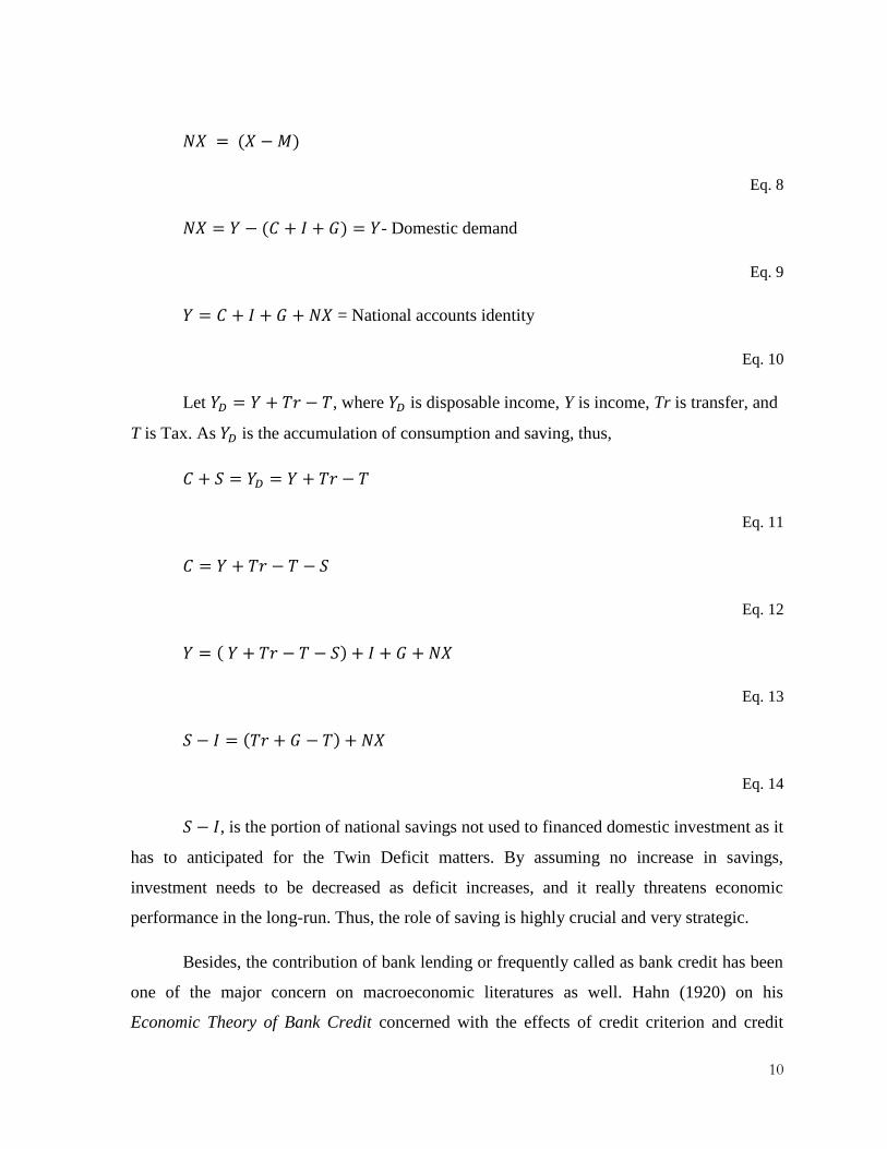
Let , where is disposable income, Y is income, Tr is transfer, and
T is Tax. As is the accumulation of consumption and saving, thus,
Eq. 11
Eq. 12
( )
Eq. 13
( )
Eq. 14
, is the portion of national savings not used to financed domestic investment as it
has to anticipated for the Twin Deficit matters. By assuming no increase in savings,
investment needs to be decreased as deficit increases, and it really threatens economic
performance in the long-run. Thus, the role of saving is highly crucial and very strategic.
Besides, the contribution of bank lending or frequently called as bank credit has been
one of the major concern on macroeconomic literatures as well. Hahn (1920) on his
Economic Theory of Bank Credit concerned with the effects of credit criterion and credit

11
extension on production. From the beginning, he believed that bank credit has the importance
of a stimulus of the conjuncture. In an advance economy with highly developed credit
institutions, which can grant loans in excess of the amount of savings deposited, the money
supply is completely elastic being “more and more inclined to accommodate itself to the
level of demand. In such an organized credit economy stability of the price level requires
equality between the natural (equilibrium) rate and the money rate of interest, i.e. the rate of
interest charged on loans. Discrepancies between the two rates lead to cumulative process.
The financing of production is essentially performed by the creation and destruction
of credit. Schumpeter shares Wicksell‟s view that the disturbance of economic equilibrium
primarily emerges from an enlargement of profitable investment options due to technical
progress rather than by an artificial lowering of the money rate of interest by the banks which
thereby causes a period of expansion which is unsustainable. Hahn (1920) concluded that
every expansion of credit results in an expansion of goods because of a change in its
distribution. Credit takes the goods out of nothing where they would have remained without
credit expansion. He suggested that expansion of credit means nothing else than an increase
of demand for goods leading to an expansion of production since, as Hahn implicitly assumes
to be the case, unemployed resources are available. Hahn (1920) emphasizes, as later
Keynes, the deflationary consequences of voluntary savings and the positive effects of an
expansionary credit policy for innovations and employment. Afterwards, Hahn (1920) began
his research of the influence of credit on capital, the core and most revolutionary part of
Economic Theory of Bank Credit with the dictum “Capital formation is not the result of
saving but of the granting of credit.” He suggested that credit constitutes the conditio sine
qua non4 of the production of commodities and all capital formation in a modern economy.
His insights are subsequently summarized in the following ideas. The first is the
limits to inflationary credit expansion in the long run. The second is that a consequence of
4 Condition sine qua non literally means an indispensable or essential ingredient or condition, without which
something could not have happened or existed. There are a number of situations when the phrase "conditio sine
qua non" applies. Anytime something would not have happened unless something else happened first, the
predicating event is said to be conditio sine qua non. (http://www.wisegeek.com/what-does-conditio-sine-qua-
non-mean.htm). Ladislaus von Bortkiewicz has aptly summarized Hahn‟s (1920) main thesis in the statement,
“Am Anfang war die Schuld” or “In the beginning was the debt”

12
the autonomous credit creation power of banks which makes possible the conjunctures, an
“economic theory of bank credit” must be formulated as a business-cycle theory. The third is
that Credit expansions may help to overcome depressions, but they should never be used in
boom periods to perpetuate them or to make bearable structural maladjustments, particularly
excessive wages. “A timely stabilization of the conjuncture, not their stimulation on and on
by inflation is desirable.” And the last is a failure in the limit of credit expansion results in
progressive inflation and a possible ruin of state finances.
According to Hahn the activity of banks consists in functioning as guarantors, i.e. to
procure trust for debtors. Money and credit markets therefore are nothing else than markets
on which credit in the literal sense of trust is traded. Credit expansion does not only affect
distribution but also production. Inflationary credit expansion leads to an increase in overall
demand which on its part stimulates the production of goods. Hahn considers the economic
“organism” as “elastic” so that hitherto underutilized resources could be activated.
Nevertheless, Schumpeter (1931), in a remarkable contrast to Hahn the credit system does
not play the role of an active producer of business cycles but rather a passive role.
2.2. The Role of Saving on Growth
Determinant of economic growth have been a great ever-lasting debate among economists
from the modern down of the profession (Noy and Nualsri, 2007). Robert Solow‟s (1956)
model has been widely used as a theoretical framework for understanding cross-country
growth patterns (McQuinn and Whelan, 2006). The model has two key points, where the first
assuming that the economy can be classified with a neoclassical aggregate production with
exogenous technological dynamics. Thus, we adopt the model with a Cobb-Douglas
aggregate production function as follow:
( )
Eq. 15

13
Where is aggregate output, is capital, is the number of labors, and is exogenous
labor-augmenting technological changes. The second key point assumes the capital stock
accumulates according to the following equation:
Eq. 16
Where s is investment share of output also assumed to be exogenous. The properties of this
model can perhaps be better understood by using a reformulated version of the production
function derived as follows:
Eq. 17
Where output per worker can be expressed as
( )
Eq. 18
This is the decomposition of output per worker into technology and capital-output
components referred to the introduction. If we denote the growth rates of technology and the
number of workers as g and n respectively, then one can easily combine the separate
dynamics for output and capital to obtain the dynamics of the capital-output ratio as:
( )
Eq. 19
where

14
( )( )
Eq. 20
and
( )
Eq. 21
These results provide a simple analytical formulation of the Solow model‟s long-run
predictions as well as its shorter-run dynamics. The capital-output ration tends to coverage
over time at rate to an equilibrium level that is a function of the investment s, the growth
rate of technology g, the growth in the number of workers n and the depreciation rate . Once
the economy has reached this value for the capital-output ratio, output per worker then grows
at the rate g given by the rate of labor augmenting technological progress.
That the equilibrium level of the capital-output ratio is independent of the level of
is a key advantage of equation (4) as a decomposition of the determinants of growth. In
contrast, the more familiar decomposition of output per worker into technology and capital-
per-worker terms suffers from disadvantage that capital-per-worker depends positively on
in the long-run, making it more difficult to disentangle the long-run effects of technology and
non-technology factors.
To understand the link between capital-output dynamics and output per worker
dynamics, it is useful to note that the log of capital-output ratio can also be approximated as
displaying a simple convergence property. In other words, letting be the log of this ratio,
then
(
) ( )
Eq. 22

15
This result allows for a simple characterization of the dynamics of output per worker.
Again letting lower case letters represent logged variables, we can take logs of equation (4)
to get
( )
Eq. 23
The steady-state path for output per worker is defined as the level of output per
worker consistent with the capital-output ratio being at its equilibrium level:
( )
Eq. 24
Using equation (8), output per worker dynamics can be expressed as
( )
Eq. 25
Thus, the convergence speed, , of the capital-output ratio is also the so-called
conditional convergence speed of output-per-worker. In other words, this is the speed at
which output-per-worker closes has two components to it: Growth is determined by
technological progress as well as the gap between and . In contrast, movements in the
capital-output ratio are determined only by the gap between output and its steady state level.

16
Figure 1 Solow Growth Model and Population Growth Rate Change
Source: Wikipedia Exogenous Growth Model5
2.3. Existing Literatures
Determinant of GDP has been widely discussed through many existing literatures, including
the contribution of savings and loan on GDP. Aghion, Comin, and Howitt (2009) believe that
savings, especially domestic, really a matter for innovation and therefore growth as it enables
the local entrepreneur who is familiar with local conditions. A cross-country regressions
show that lagged is positively related to productivity growth in poor countries but not in rich
countries. They develop a theory that of endogenous local saving and growth in an open
economy with domestic and foreign investor. They explained that growth in relatively poor
countries results mainly from innovations that allow local sectors to catch up with the current
frontier technology. However, catching up with the frontier in any sector requires the
cooperation of foreign investors who is familiar with the frontier technology and a domestic
entrepreneur who is familiar with the local conditions to which technology must be adapted.
In such country, domestic saving matters for technology adoption, and therefore growth as it
allows the local entrepreneur to take an equity stake in this cooperative venture, which
mitigates an agency that would otherwise discourage the foreign investors from participating.
The dependent variable is a measure of growth of productivity (TFP) while independent
5 http://chula.livocity.com/econ/Macro%20Charit%20-
%20Paitoon/Charit%20too/Exogenous_growth_model.htm accessed Wednesday, 11 December 2013, 14.31

17
variable of interest is the average saving rate in ten-year period using OLS estimation
technique.
Al Foul (2010) conducted an analysis on causal long-run relationship between
savings and economic growth from MENA countries. The research observed two countries,
Morocco (1965-2007) and Tunisa (1961-2007) using a newly developed approach to
cointegration namely Autoregressive Distributed Lag (ARDL) considering each variable as a
dependent variable by Pesaran et al. (2001) that performs well with small samples and
regardless of the orders of the respective time series (i.e., whether time series are I(0), I(1), or
I(0)/I(1). The results showed that the long-run relationship exist between variables in the case
of Morocco, while it was not proven in Tunisia. By employing Granger causality test, Al
Foul (2010) found bidirectional relationship in Morocco while in the case of Tunisia, the
results suggest that there is unidirectional ganger causality between real GDP and real Gross
Domestic Savings and runs from saving growth to economic growth.
Caroll and Weil (1994) examine the relationship between income growth and saving
using both cross-country and household data. They examined the panel of non-overlapping
five year averages of saving and growth. They used model of consumption with habit
formation as standard permanent income models cannot explain these findings. They, firstly,
found that growth causes savings while savings do not lead growth. Secondly, those
household who expect faster income growth appear to save more than households who
should expect slower income growth.
Saltz (1999) investigates the long-run relationship between saving and economic
growth in 17 developing countries. He identified the existing bidirectional relationship
between variables among the countries. He found 4 countries have causal relationship from
saving to the real GDP while 10 countries have the reverse causal relationship from
economic growth to saving.
Claus, Haugh, Scobie, and Tornquist (2002) investigate the link between savings,
investment, and growth in New Zealand. In an open economy, total saving comprises saving
by domestic agents (government, firms, and households) plus foreign saving. Diversified

18
portfolios, large inflows of foreign investment into New Zealand and investment rates
comparable to those in OECD countries suggest that New Zealand has been able to access
foreign saving to meet investment demands. For this case, they employed net national
savings, total gross capital formation (investment), the current account, and real GDP growth
for 12 selected OECD countries from 1972-2001. For the New Zealand experience, they
applied the variables used to compare with OECD countries except investment employing
OLS estimation technique. They found that savings a positive and significant long-run
relationship to GDP growth while applying Granger causality test, they found that savings
and growth have a bidirectional relationship. Nevertheless, higher income led to the decrease
of savings as household preferred to increase their consumption (thus lowering savings (in
anticipation of higher output growth in the future.
The research work by Swiston (2008) on the USA used a VAR containing two lags to
construct a model with variables such as nominal interest rate, yield on investment grade
corporate bonds with remaining maturity of 5-10 years to capture long term interest rate, real
GDP, oil prices, equity returns and real effective exchange rate made positive contribution in
that direction. He posited that credit availability proxied by survey results on lending
standards is an important driver of the business cycle, accounting for over 20% of the typical
contribution of financial factors to growth. A net tightening in lending standards of 20%
basis points reduces economic activity by ¾% after one year and 1¼% after two years.
Hevia and Loayza (2011) investigated long-run relationship between savings and loan
in Egypt. They focused on illustrating the mechanism linking national saving and economic
growth, with the purpose of understanding the possibilities and limits of saving-based growth
agenda in the context of the Egyptian economy. They conducted complementary simulations,
firstly, the one designed to measure the savings rates required to finance a given rate of
economic growth set to 4% of GDP growth per worker. In that case, investment need to
increase by 37% of GDP as the marginal return to capital decreases, thus national savings
need to increase by, first 35% of GDP, then 50% in 10 years, and almost 80% by the end of
25-year period to promote economic growth. Secondly, what economic growth rates can be
financed if the saving rate is fixed at a given rate, set to 20% of national saving to GDP. They

19
found that the growth rate of GDP per worker will start at 0.8%, and then decrease gradually
to 0.7% in 25 years as explained by diminishing returns to capital which is constant rate in
this simulation. The simulation has proven that higher national savings would lead
remarkable growth performance, as occurred in China.
In the case of the long-run relationship between savings and growth in China, Lean
and Song (2008) conducted the investigation in four representative provinces, i.e. Beijing,
Shanghai, Guizhou, and Xinjiang covering the period from 1955 to 2004. By applying
Johansen-Juselius (1990) cointegration test, they found that China;s economy seems to be
contegrated with household savings and enterprise savings. By applying granger causality
test based on Vector Error Correction Model (VECM), household savings and economic
growth performed bidirectional relationship in the short-run while in the long run,
unidirectional causality exist from economic growth to the enterprise saving growth all
samples.
Loans or credit distributions also become the main concern in the paper. Cappiello,
Kadareja, Saensen, and Patropapa (2010) examined whether bank loans and credit standard
have an effect on output focusing on the Euro area such as Austria, Belgium, Greece, Ireland,
Italy, Netherland, Portugal, and Spain. They employ quarterly data from 1999 to 2008 for
nominal GDP, real GDP, GDP deflator, money (M3 less currency and M2 minus currency
and time deposit). In contrast to the US findings, changes in the supply of credit, both in
terms of volumes and credit standards applied on loans to enterprises, have significant effects
on real economic activities by applying OLS panel regressions.
Interestingly, other findings have been observed in Nigerian case by Oluitan (2010).
He used bivariate model as proposed by Ghirmay (2004) on his research in 16 Sub-Saharan
Africa countries and multivariate model proposed by Tang (2003) on his research about bank
lending and economic growth in Malaysia. He examined the relationship by applying
cointegration test and direction of causality using Error Correction Method (ECM) and OLS
estimation technique. The following variables are real GDP, real private sector credit, real
total export, GDP Per Capita, Ratio of Bank Deposit to GDP, and Private Sector Deposit to
GDP. He found that the autoregressive coefficient for the real private sector credit growth

20
was negative, large, and significant in all the results, but the first model that tested the
bivariate relationship between credit and real output showed a positive coefficient. It implies
that the relationship among all these variables is weak.
Nevertheless, a discussion on gross domestic cannot be separated from other
determinants. Economists have found that Foreign Direct Investment (FDI), Domestic Direct
Investment (DDI), Human Capital, Inflation, Trade Openness, and Population are the
frequent determinants in many economic literatures. Alfaro (2003) examined the link
between FDI and Economic Growth. He found that FDI contributes various relationships on
growth in primary, manufacturing, and service sectors. He uses an empirical analysis using
cross-country data from different regions (e.g. Asia and the Pacific, Africa, Latin America,
and the Caribbean) for the period 1981-1999 and found a positive relationship between FDI
and growth mainly in manufacturing sector while it tends to be ambiguous as primary sectors
perform negative relationship. As confirmed by Anwar and Nguyen (2010) focusing on
Vietnam case, the relationship FDI on growth tends to be positive and significant. Moreover,
the effect would be higher if the investment is addressed, mainly, to education and training to
improve the local qualification and generate more output in the long-run. The role of
education (or in general, of the formation of human capital) in the growth process has been
extensively analyzed in the theory literature (Nelson and Phelps, 1996; Welch, 1970; Lucas,
1988; Azariadis and Drazen, 1990; and Romer, 1990; among others).
Seren (2001) examined how human capital affects growth estimating pooled data for
different samples of countries during the period 1960-1990 divided into five-year intervals.
She observed using the following data, income, population, labor force, and investment rates.
She found various significance and positive relationship between human capital and growth.
Meanwhile, inflation rate and trade openness is also a primary concern in economic growth.
Betyak (2012) examined some determinants of economic growth in, especially, crisis
countries in European Union. Using least square panel regression analysis, he found that
inflation rate has a positive relationship in the case of Portugal, Italy, Ireland, and Spain.
Interestingly, the relationship is negative in the case of Greece. Meanwhile, trade openness

21
has been positively related to GDP growth in Portugal, Italy, and Spain while Greece seems
to be negative.
Besides, the analysis of determinant of GDP based on economic activities-based
sector also becomes the primary concern to generate accurate selected contributions on GDP.
Burgess (2011) measured financial sector output and its contribution to UK GDP. By
observing some financial service industries such as monetary intermediation, insurance
companies, pension funds, and activities auxiliary to financial intermediation, he found
insignificant relationship between financial output sectors on GDP.
Furthermore, Diao, Hazell, Resnick, and Thurlow (2007) investigated the role of
agriculture in development focusing on the implications for Sub-Saharan Africa. By
examining different typology of agricultural conditions, natural resources, and geographic
location, they found that growth potential and poverty reduction potential of agriculture
varies substantially across continents. They found that agriculture growth is till important for
most-low African countries. As stated in the previous research, Vodel (1994) observed
different 27 countries in terms of agriculture contribution in growth. Using social accounting
matrixes, he found that significant relationship appeared in the early stages, while the
forward linkages are much weaker.
Moreover, Arcand (2000) shows that the link between nutrition (agriculture product)
and economic growth is robust to the use of different data sets and different econometric
techniques, ranging from OLS to GMM. Using three different cross-county data sets, he
found that nutrition affects growth directly, through labor productivity, and indirectly,
through improvements of life expectancy.
Anyanwu, Offor, Adesope, and Ibekwe (2013) observed the relationship between
GDP and agriculture, industry, building and construction, wholesale and retail, and trade and
services share of GDP. By employing multiple regression, they found that agriculture had
been dominant since 1960 to 1989 while industry contributed more on GDP started from
1990 to 2008. Building and construction remained to contribute least to GDP throughout the

22
period of observation. However, some significant determinants on GDP were agriculture,
industry, wholesale and retail trade, and service sectors.
Strategic Finance Group (2007) on economic frontier analyzed the association
between unexpected changes in electricity volume and GDP growth for residential
customers. They employ several data such as real GDP, electricity price, and gas prices. They
apply Vector Error-Correction Model (VECM) to describe the long-run and the short-rum
relationship between the two time-series employed. Using simple linear regression
estimation, GDO growth and growth in electricity volumes suggest that the elasticity of
volume growth to GDP may be significantly less than one (few changes on volume leads
huge changes in GDP growth).
Based on theoretical grounds and literatures study we build empirical model to
estimate on this paper. The specification of proposed model and its variants will be discussed
on the next session of this paper.
3 METHODOLOGY
3.1. Empirical Model
The paper investigates the long-run relationship among savings and loans on gross domestic
product of Indonesia from 1988 to 2012. It is considered important to observe bidirectional
relationship between savings, loans, and gross domestic product of Indonesia. Granger
causality test is also employed to identify long-run bidirectional relationship between
savings, loans, and gross domestic product of Indonesia.
The paper employs three independent variables while six others are determined as the
controlling variables. Interestingly, the paper uses both panel and time series to analyze the
long-run relationship between desired independent variables and Indonesia‟s output. As loans
for investment and working capital are detailed by its cross-sections, thus it will be analyzed
using panel approach in order to provide more accurate output (Greene, 2010) with the
following model:

23
Eq. 26
Where is Gross Domestic Product, is a set of dependent variables (loan for
investment and working capital), is a set of control variables such as FDI, DDI, and labor
by sector, and is the error term.
As savings and loan for consumption are not detailed by sector of real economic
activities, they will be analyzed using the following time series model.
Eq. 27
Where is Gross Domestic Product, is a set of dependent variables (loan for investment,
working capital, consumption, and savings), is a set of control variables such as FDI,
DDI, years of schooling and labor by sector, and is the error term.
3.2. Data
Referring to Solow Model, the following variables have been determined accordingly, and
based on the frequent previous literatures. The theory included capital proxied by FDI, DDI,
Savings and Loans while human capital aspects are proxied by labor-based nine economic
activities, school participation rate, and years of schooling. Meanwhile, as stated in the
frequently previous literatures, trade openness, inflation, and population are added to the
model.

24
Table 1. Variable and Data
Variables Names Units Sources
Dependent GPD/Labor Nominal Bank Indonesia
Independents Savings Billion Rp Bank Indonesia
Loan for Investment Billion Rp Bank Indonesia
Loan for Working Capital Billion Rp Bank Indonesia
Loan for Consumption Billion Rp Bank Indonesia
Controls FDI Billion Rp Investment Coordination Board
DDI Billion Rp Investment Coordination Board
School Participation Rate Percentage (%) National Bureau of Statistics
Population Growth Percentage (%) Index Mundi
The following variables are estimated using panel approach. As saving and loan for
consumption is not detailed by sector-based real economic activities, thus we also employ
time series approach. Time series as being utilized in the model, is a set of data that is
collected sequentially in time (Reinert, 2010).
3.3. Panel Data Estimation
Panel data is a data sets consisting of multiple observations on each sampling unit (Baltagi,
2006). Panel data are a type of longitudinal data (Hsiao 2003). In other words, we can further
explain that data panel contains two or more observations on many units. Data panel has been
very popular in many research on social and behavior field. It is repeated measures of one or
more variables on one more persons-repeated cross-sectional time series (Bruderl, 2005).
Compared to the other two types of data (time series and cross section), data panel has
several benefits like being able to control the heterogeneity of individual, providing complete

25
data with low level of colinearity and higher degree of freedom, appropriate to examine
dynamics of adjustments, more reliable to identify and measure both individual and time
effect that cannot be solved by time series and cross section data, and appropriate to build
and test a model with complex behavior. A panel data set also allows us to control for
unobserved cross section heterogeneity (Wooldridge, 2001)
Hurlin (2010) described the terminology and notations are explained by through
individual or cross section unit that could be country, region, state, form, consumer,
individual, couple of individuals or countries (gravity model6) and also double index where
is cross-section unit and is the series of time.
where and are and vectors of exogenous variables. is constant, and
are and vectors of parameters. is over and , with ( ) . It is
noted that variables unobservable and correlated with (Baltagi and Kao, 2000)
3.3.1. Alternative Specification
As mentioned above, data panel is a combination between time series and cross section so
that data panel modeling involves the two characteristics of those two types of data. Data
panel basically involves more than one objects and observations (Winarno, 2009). According
to Nachrowi (2006) data panel regression model uses some of the following approaches.
3.3.1.1. Generalized Least Square
Generalized Least Square is introduced to improve upon estimation efficiency when var(y) is
not a scalar variance-covariance matrix (Fox, 2002). GLS is then becoming an alternative as
OLS is inefficient since disturbances are nonspherical7. A drawback of the GLS method is
that it is difficult to implement. In practice, certain structures (assumptions) must be imposed
6 In economics, gravity model is the standard of non-zero trade flows in macroeconomics
(http://arxiv.org/abs/1304.3252) 7 Spherical disturbance means the variance of error is equal to population variance

26
on ( ) so that a feasible GLS estimator can be computed8. This approach results in two
further difficulties, however. First, the postulated structures on var(y) need not be correctly
specified. Consequently, the resulting feasible GLS estimator may not be as efficient as one
would like. Second, the finite-sample properties of feasible GLS estimators are not easy to
establish. Consequently, exact tests based on the feasible GLS estimation results are not
readily available.
Often we have analysis situations where it is unreasonable to assume that our errors
are independent and identically distributed. Heteroskedasticity, that is unequal variances of
the error term, may be a problem. It is also common to have data where errors are correlated
(Winship, 2007)
In a typical linear regression model we observe data { }
on n statistical units. The response values are placed in a vector ( ), and the
predictor values are placed in the design matrix [ ], where is the value of the jth
predictor variable for the ith unit. The model assumes that the conditional mean of Y given X
is a linear function of X, whereas the conditional variance of the error term given X is a
known matrix Ω. This is usually written as
⌈( | )⌉ ⌈( | )⌉
Eq. 28
Here β is a vector of unknown “regression coefficients” that must be estimated from
the data.Suppose b is a candidate estimate for β. Then the residual vector for b will be
Y − Xb. Generalized least squares, which is two steps from Ordinary Least Squares, method
estimates β by minimizing the squared Mahalanobis9 length of this residual vector:
( ) ( )
Eq. 29
8 Generalized Least Square requires two following assumptions. The first is the covariance of error is diagonal,
and the second is the structure of error covariance of error is observable 9 Descriptive statistic that provides a relative measure of data point‟s distance (residual) from a common point.

27
Since the objective is a quadratic form in b, the estimator has an explicit formula:
( )
Eq. 30
The GLS estimator is unbiased, consistent, efficient, and asymptotically normal:
√ ( ) → ( ( ) )
Eq. 31
GLS is equivalent to applying ordinary least squares to a linearly transformed version
of the data. To see this, factor , for instance using the Cholesky decomposition. Then
if we multiply both sides of the equation by , we get an equivalent linear
model where , and . In this
model , - ( ) . Thus we can efficiently estimate β by applying OLS to
the transformed data, which requires minimizing:
( ) ( ) ( ) ( )
Eq. 32
This has the effect of standardizing the scale of the errors and “de-correlating” them.
Since OLS is applied to data with homoscedastic errors, the Gauss–Markov theorem10
applies, and therefore the GLS estimate is the best linear unbiased estimator for β. Or in other
words, it can be said to be essentially useful, through transformation, to change from
heteroscedastic to homoscedastic.
3.3.1.2. Fixed Effect Model
Fixed Effect Model is a statistical model that represents the observed quantities in terms of
explanatory variables that are treated as if the quantities were non-random (Peter, Patrick,
Yee, and Scott, 2002). This is in contrast to random effects models and mixed models in
10
Stating that a linear regression model has expected zero errors and are uncorrelated as well as having equal
variances.

28
which either all or some of the explanatory variables are treated as if they arise from random
causes. Contrast this to the biostatistics definitions, as biostatisticians use "fixed" and
"random" effects to respectively refer to the population-average and subject-specific effects
(and where the latter are generally assumed to be unknown, latent variables).
Fixed effect model can be mathematically explained as follow:
Eq. 33
where is the dependent variable observed for individual i at time k, is the time-variant
regressor matrix, is the observed time-invariant11
individual effect and is the error
term. Unlike , cannot be observed by the econometrician. Common examples for
time-invariant effects are innate ability for individuals or historical and institutional
factors for countries. The fixed effect model allows to be correlated with the regressors
matrix . Strict exogeneity, however, is still required.
Since is not observable, it cannot be directly controlled for. The Fixed Effect
model eliminates by demeaning the variables using the within transformation:
( ) ( ) ( )
Eq. 34
Where
∑
and
∑
. Since is constant, and hence the effect
is eliminated. The fixed effect estimator is then obtained by an OLS regression of on
. Another alternative to the within transformation is to add a dummy variable for each
individual i. This is numerically, but not computationally, equivalent to the fixed effect
model and only works if T, the number of time observations per individual, is much larger
than the number of individuals in the panel.
11
Time-variant individual means identifier specific characteristic of is fixed.

29
3.3.1.3. Random Effect Model
Random Effect Model is intended to differ between individual or period effect, so that
intercept of the equation is the average of the intercept of the overall observations (Peter,
Patrick, Yee, and Scott, 2002). In statistics, a random effect(s) model, also called a variance
components model, is a kind of hierarchical linear model. It assumes that the dataset being
analyzed consists of a hierarchy of different populations whose differences relate to that
hierarchy. In econometrics, random effects models are used in the analysis of hierarchical or
panel data when one assumes no fixed effects (i.e. no individual effects). The random effect
model can be mathematically expressed as follow
Eq. 35
where all variables are defined as above. At first glance this appears the same as equation
(general model), but there are differences. First, the random effects model assumes that the
effects of , and on do not change over time. This is why (not subscript)
replaces and replaces . Second, the random effects model assumes that is a
random latent variable that is uncorrelated with , , and . Considering the type of
unmeasured time-invariant variables that might appear in (e.g. intelligence, personality with
all other explanatory variables in the analysis. If this assumption or the assumption of the
same coefficients over time is incorrectly imposed, either can bias the estimated effects that
we find. Another assumption of the random effects model is that the error variance does not
change over time (
). Violation of this assumption can lead to inaccuracy of the
estimates (Bollend and Brand, 2008).
One common estimator of the coefficients and variances of the error and time-
invariant latent variable is the feasible Generalized Least Square (GLS) estimator (e.g. Hasio,
2003; and Woldridge, 2002). In this approach, an estimate of the variance of and of are
used to form the “weight matrix” for GLS estimation. If the preceding assumptions hold, then
this procedure has desirable large sample properties such as consistency, asymptotic
unbiasedness, and readily available significance tests. It also provides an estimate and test of

30
whether there are latent time-invariant variables ( ) such that zero variance of
implies their absence. A maximum likelihood estimator of the random effects model also is
possible under the assumption that and come from a normal distribution (Hsiao, 2003).
One or both of these estimators are available in statistical software such as SAS (e.g.
TSCSREG) or STATA (xtreg). However, the use of these procedures presupposes that the
assumptions of the random effect model hold, with the assumption that the latent time-
invariant variable is uncorrelated with all observed covariates being the most problematic
assumption. The fixed effect model removes this restriction.
Implicit in the summary-statistics of Random Effect Model approach is the two-level
model
Eq. 36
Eq. 37
where is the true mean effect for the subject , is the sample mean effect for subject
and is the true effect for the population.
The Summary-Statistic (SS) approach is of interest because it is computationally
much simpler to implement than the full random effects model of equation 1. This is because
it is based on the sample mean value, , rather than on all of the samples . This is
important for neuroimaging as in a typical functional imaging group study there can be
thousands of images, each containing tens of thousands of voxels. In the first level we
consider the variation of the sample mean for each subject around the true mean for each
subject. The corresponding variance is , -
, where
is the within-subject variance.
At the second level we consider the variation of the true subject means about the population
means where about the population mean where , - the between-subject variance.
We also have , - , - . Consequently,
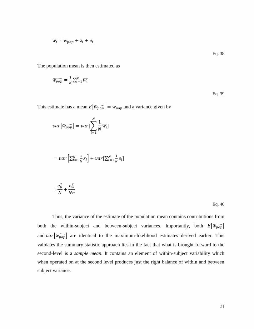
31
Eq. 38
The population mean is then estimated as
∑
Eq. 39
This estimate has a mean [ ] and a variance given by
[ ] ,∑
-
[∑
] ,∑
-
Eq. 40
Thus, the variance of the estimate of the population mean contains contributions from
both the within-subject and between-subject variances. Importantly, both [ ]
and [ ] are identical to the maximum-likelihood estimates derived earlier. This
validates the summary-statistic approach lies in the fact that what is brought forward to the
second-level is a sample mean. It contains an element of within-subject variability which
when operated on at the second level produces just the right balance of within and between
subject variance.

32
3.3.2. Determining the Best Model
In panel analysis using Ordinary Least Square estimation technique, there are some following
statistical tests to determine the best model of an analysis such as Chow Test, LM test and
Hausman Test (Nachrowi, 2006) as follow:
3.3.2.1. Chow Test
The Chow test is a statistical and econometric test of whether the coefficients in two linear
regressions on different data sets are equal. The Chow test was invented by economist
Gregory Chow in 1960. In econometrics, the Chow test is most commonly used in time series
analysis to test for the presence of a structural break. In program evaluation, the Chow test is
often used to determine whether the independent variables have different impacts on different
subgroups of the population (Doughterty and Christoper, 2007).
The Chow Test can be mathematically explained as follow:
Eq. 41
and
Eq. 42
The null hypothesis of the Chow test asserts that , , and , there is
the assumption that the model errors are independent and identically distributed from a
normal distribution with unknown variance
Let be the sum of squared residuals from the combined data, be the sum of
squared residuals from the first group, and be the sum of squared residuals from the
second group. and are the number of observations in each group and k is the total
number of parameters. Then the Chow test statistics is:

33
Chow Stat ( ( )) ( )⁄
( ) ( )⁄
Eq. 43
The test statistic follows the F distribution with k and ( ) degrees of
freedom.Related to determine to use either Pooled Least Square of Fixed Effect Model
estimation, then reject the null hypothesis ( ) if the p-value is less than the
critical value.
3.3.2.2. LM Test
The Lagrange Multiplier (LM) test is a general principle for testing hypotheses about
parameters in a likelihood framework (Cook and Demets, 2007). The hypothesis under test is
expressed as one or more constraints on the values of parameters. To perform an LM test
only estimation of the parameters subject to the restrictions is required. This is in contrast
with Wald tests, which are based on unrestricted estimates, and likelihood ratio tests which
require both restricted and unrestricted estimates.
The name of the test is motivated by the fact that it can be regarded as testing whether
the Lagrange multipliers involved in enforcing the restrictions are significantly different from
zero. The term “Lagrange multiplier” itself is a wider mathematical word coined after the
work of the eighteenth century mathematician Joseph Louis Lagrange. The LM testing
principle has found wide applicability to many problems of interest in econometrics.
Moreover, the notion of testing the cost of imposing the restrictions, although originally
formulated in a likelihood framework, has been extended to other estimation environments,
including method of moments and robust estimation. Statistically, it can be explained as
follow:
Let ( ) be a log-likelihood function of a parameter vector , and let the score
function and the information matrix be
( )

34
Eq. 44
( ) , ( )
-
Let be the maximum likelihood estimator (MLE) of subject to an vwctor of
constraints ( ) . If we consider the Lagrangian function
( ) ( )
Eq. 45
where is an vector of Lagrange multipliers, the first-order conditions for are
( ) ( )
( )
Eq. 46
where ( ) ( )
The Lagrange Multiplier test statistic is given by
Eq. 47
where ( ), ( ), and ( ). The term is the score form of the statistic
is the Lagrange multiplier form of the statistic. They correspond to two different
interpretations of the same quantity.

35
The score function ( ) is exactly equal to zero when evaluated at the unrestricted MLE
of , but not when evaluated at ( ). If the constraints are true we would expect both and to
be small quantities, so that the region of rejection of the null hypothesis ( ) is
associated with large values of LM. Under suitable regularity conditions, the large-sample
distribution of the LM statistic converges to a chi-square distribution with degrees of
freedom, provided the constraints ( ) are satisfied. This result is used to determine
asymptotic rejection intervals and p-values for the test. Breusch Pagan Lagrange Multiplier
LM test is intended to determine the best model between Pooled Least Square (PLS) and
Random Effect Model (REM).
3.3.2.3. Hausman Test
Consider the linear model y = bX + e, where y is univariate and X is vector of regressors, b is
a vector of coefficients and e is the error term (Greene, 2008). We have two estimators for b:
b0 and b1. Under the null hypothesis, both of these estimators are consistent, but b1 is
efficient (has the smallest asymptotic variance), at least in the class of estimators containing
b0. Under the alternative hypothesis, b0 is consistent, whereas b1 isn‟t.
Then the Wu–Hausman statistic is
( ) ( ( ) ( ))
( )
Eq. 48
Where + denotes the Moore–Penrose pseudoinverse12
. This statistic has asymptotically the
chi-squared distribution with the number of degrees of freedom equal to the rank of matrix
Var(b0) − Var(b1). If we reject the null hypothesis, b1 is inconsistent. This test can be used to
check for the endogeneity of a variable (by comparing instrumental variable (IV) estimates to
ordinary least squares (OLS) estimates). It can also be used to check the validity of extra
instruments by comparing IV estimates using a full set of instruments Z to IV estimates that
use a proper subset of Z. Note that in order for the test to work in the latter case, we must be
12
Moore-Penrose Pseudoinverse is defined for any matrix and is unique. It brings great notational and
conceptual clarity to the study of solutions to arbitrary systems of linear equations and linear least squares
problems (Soderstorm, Torsten; Stewart, G.W. (1974)

36
certain of the validity of the subset of Z and that subset must have enough instruments to
identify the parameters of the equation. Hausman also showed that the covariance between an
efficient estimator and the difference of an efficient and inefficient estimator is zero.
Related to determine to choose either fixed effect or random effect through hausman
test. The null hypothesis states that is is uncorrelated with the variables in , then
random effects is the appropriate estimator, while if correlated with the variables in ,
then fixed effects is the appropriate estimator. The Hausman test can be statistically
explained by the following model:
[ - ], ( ) ( )- [ -
]
Eq. 49
3.4. Parameter Estimation
3.4.1. Ordinary Least Square
The least square method is widely used to find or estimate the numerical values of the
parameters to fit a function to a set of data and to characterize the statistical properties of
estimates. It exists with several variations (Abdi, 2003). Ordinary least square is a
generalized linear modeling technique that may be used to model a single response variable
which has been recorded on at least an interval scale. It can be applied to single or multiple
explanatory variables and also categories explanatory that have been appropriately coded. At
a very basic level, the relationship between a continuous response variable (Y) and a
continuous explanatory variable (X) may be represented using a line of best-fit. If this
relationship is linear, it may be appropriately represented mathematically using the straight
equation .
In addition to the model parameters and confidence intervals for , it is useful to laso
have an indication of how well the model fits the data. It can be determined by comparing the
observed the scores of Y (the values of Y predicted by the regression equation). The

37
difference between the two variables (the deviation, or residual as it is also called) provides
an indication of how well the model predicts each data point. The sum of all squared
residuals is known as the residual sum of squares (RSS) and provides a measure of model-fit
for an OLS regression model. A poorly fitting model will deviate markedly from the data and
will consequently have a relatively large RSS and vice versa (a perfectly fitting model will
have an RSS equal to zero, as there will be no deviation between observed and expected
values of Y).
It is important to understand how the RSS statistic (Hutchseson, 2011) operates as it
is used to determine the significance of individual and groups of variables in a regression
model. For a simple OLS regression model, the effect of the explanatory variable can be
assessed by comparing the RSS statistic for the full regression model with that
for the null model . The difference in deviance between the nested models can be tested
for significance using an F-test computed from the following equations:
( )(
)
Eq. 50
where p represents the null model, , p+q represents the model , and df are
the degrees of freedom associated with the designated model. It can be seen from equation
that the F-statistic is simply based on the difference in the deviances between the two models
as a fraction of the deviance of the full model, whilst taking account of the number of
parameters.
In order to explain the efficient Ordinary Least Square, we start by the following
equations:
Eq. 51
, -

38
Eq. 52
, -
Eq. 53
is full-rank and contains . In this case, OLS is BLUE. So we can get an estimated
parameter vector
( )
Eq. 54
Its bias is
[( ) ] ,( ) ( )
,( ) - ( )
Eq. 55
The variance of the estimated parameter vector is the expectation of the square of the
quality in square brackets:
[ ] ,( )( ) -
,( ) ( ) -
( ) , - ( )
( ) ( )
( ) ( )
( )
Eq. 56

39
Additionally, in order to get a precise estimate, we can assume [ ] ( )
in three pieces. The first is the variance of is the variance of conditional on . Less
variation of around the regression line yields greater precision. The second is is the
number of observations. It shows up, implicitly, inside . This is easiest to see if has just
one column: in the case, ( ) ∑ ( )
which for drawn from some density ( )
has an expectation that increases linearly with . So, [ ] goes inversely proportionally
with . The thord is is related to the covariance matrix the vectors . If
each column of is mean-zero, then is the covariance matrix of the columns of . For
this reason, if has a lot of variance, then is bigger, so ( ) is smaller, so [ ] is
smaller and estimate is more precise. Here is not observed. However, we have a
sample analog, the sample residual :
Eq. 57
So we can further exactly explain how relate to by the following equation.
( )
, ( ) -
, ( ) - , ( ) -
, ( ) -
, ( ) -
Eq. 58
is a linear transformation of . However, although, ( ) - is an
matrix, it is not a full rank matrix; its columns are related. Indeed, the weighting matrix
is all driven by the identity matrix, which has rank , and the matrix , which only has
columns. The full matrix , ( ) - has rank .

40
Matrices like , ( ) - and ( ) are called projection matrices, and
they come up a lot. For any matrix , denote its projection matrix ( ) and its
error projection as ( ) . These are convenient. We can write the OLS
estimate of as
,
Eq. 59
And the OLS residual as
Eq. 60
and also
Eq. 61
We say stuff like “The matrix projects onto . These matrices have a few useful
properties such as being symmetric and idempotent, which means they equal their own
square, .
Compute in terms of :
Eq. 62
so,
, - , -
, -
41
, - , ( ) -
Eq. 63
Because has rank . Consequently,
, -
Eq. 64
So we can use an estimate
Eq. 65
The estimated variance of the OLS estimator is thus given by
[ ] ( ) .
Eq. 66
Now, we can compute the BLUE estimate, and say something about its bias (zero) and its
sampling variability if we have spherical disturbances.
3.4.2. Maximum Likelihood
The principle of maximum likelihood is relatively straightforward. As before, we begin with
a sample ( ) of random variables chosen according to one of a family of
probabilities . In addition, ( | ) ) will be used to denote the density
function for the data when is the true state of nature. Then, the principle of maximum
likelihood yields a choice of the estimator as the value of the parameter that makes the
observed data most probable. The likelihood function is the density function regarded as a
function of .

42
( | ) ( | )
Eq. 67
The maximum likelihood estimator (MLE)
( ) ( | )
Eq. 68
In a large sample, the maximum likelihood estimators have many desirable properties.
However, especially for high dimensional data, the likelihood can have many local maxima.
Thus, finding the global maximum can be a major computational challenge.
This class of estimators has an important property. If ( ) is a maximum likelihood
estimate for , then ( ( )) is a maximum likelihood estimate for ( ). For example, if
is a parameter for the variance and is the maximum likelihood estimator, then √ is the
maximum likelihood for the standard deviation. The flexibility in estimation criterion seen
here is not available in the case of unbiased estimators. Typically, maximizing the score
function, ( | ), the logarithm of the likelihood, will be easier.
3.4.3. Generalized Method of Moment
Generalized Method of Moment (GMM) is a general estimation principle. Estimators are
derived from so-called moment conditions (Nielsen, 2005). There are some motivations to
apply GMM, firstly, many estimators can be seen a s special cases of GMM unifying
framework for comparison. Secondly, maximum likelihood estimators have the smallest
variance in the class of consistent and asymptotically normal estimators; however, we need a
full description of the data generating process and correct specification. Unlike maximum
likelihood, GMM does not require complete knowledge of the distribution of the data. Only
specified moments derived from an underlying model are needed for GMM estimation.
In some cases in which the distribution of the data is known, MLE can be
computationally very burdensome whereas GM can be computationally very easy. The log-
normal stochastic volatility model is one example. In models for which there are more

43
moment conditions than model parameters, GMM estimation provides a straightforward way
to test the specification of the proposed model. This is an important feature that is unique to
GMM estimation. GMM is an alternative based on minimal assumptions. The last, GMM
estimation is often possible where a likelihood analysis is extremely difficult. We only need a
partial specification of the models for rational expectations. A moment condition is a
statement involving the data and the parameters:
( ) , ( )-
Eq. 69
where is a K x 1 vector of parameters; ( ) is an R dimensional vector of (non-linear)
functions; contains model variables; and contains instruments.
If we knew the expectation that we could solve the equation in (*) to find . If there
is a unique solution, so that
, ( )- if and only if
Eq. 70
Then we say that the system is identified. Identification is essential for doing econometrics as
applied for “is the model constructed so that is unique (identification) and are the data
informative enough to determine (empirical identification). In many applications, the
moment condition has the specific form as follow.
( ) ( )
Eq. 71
Where the R instruments in the are multiplied by the disturbance term, ( ). It can be
assumed as the equivalent of an error term. The moment condition becomes.
( ) , ( ) -
44
Eq. 72
stating that the instruments are uncorrelated with the error term of the model. This class of
estimators is referred to as instrumental variables estimators. The function ( ) may be
linear or non-linear in .
GMM estimation can frame the OLS estimation, by letting and ( )
( ), implying the following moment condition.
, - , * | +-
Eq. 73
In this set-up, the dimension of and are equal (and hence the dimension of and ( )
are equal) in the linear regression method. It can be further solved by
∑
( )
( )
( )
Eq. 74
3.5. Model Validation
3.5.1. Adjusted R-Square
All models basically need to be validated. In addition to the model-fit statistics, the R-square
statistic is also commonly quoted and provides a measure that indicates the percentage of
variation in the response variable that is explained by the model (Draper and Smith, 1998). It
is defined as

45
Eq. 75
And basically gives the percentage of the deviance in the response variable that can
be accounted for by adding the explanatory variable to the model. Although R-square is
widely used, it will always increase as variables added to the model (the deviance can only
go down when additional variables are added to a model). One solution to this problem is to
circulate an adjusted R-square statistic ( ), which takes into account the number of terms
entered into the model and does not necessarily increase as more terms are added. Adjusted
R-square can be derived using the following equation:
( )
Eq. 76
where n is the number of cases used to construct the model and k is the number of terms in
the model (not including the constant).
3.5.2. Marginal Cost of Information
3.5.2.1. Akaike Information Criterion (AIC)
The Akaike information criterion (1973) is a measure of the relative quality of a statistical
model, for a given set of data. As such, AIC provides a means for model selection. AIC deals
with the trade-off between the goodness of fit and the complexity of the model. It is founded
on information entropy: it offers a relative estimate of the information lost when a given
model is used to represent the process that generates the data. Burnham and Anderson (2002)
suggested that Akaike Information Criterion (AIC) is a way of selecting a model from a set
of models. The chosen model is the one that minimizes the Kullback-Leibler distance
between the model and the truth. It's based on information theory, but a heuristic way to
think about it is as a criterion that seeks a model that has a good fit to the truth but few
parameters. It is defined as:
( ( ))
Eq. 77

46
where likelihood is the probability of the data given a model and K is the number of free
parameters in the model. AIC scores are often shown as ∆AIC scores, or difference between
the best model (smallest AIC) and each model (so the best model has a ∆AIC of zero). The
second order information criterion, often called AICc, takes into account sample size by,
essentially, increasing the relative penalty for model complexity with small data sets. It is
defined as:
( ( )) ( ( ))
Eq. 78
where n is the sample size. As n gets larger, AICc converges to AIC ( n - K -1 -> n as n gets
much bigger than K, and so (n / ( n - K - 1)) approaches 1), and so there's really no harm in
always using AICc regardless of sample size. In phylogenetics, defining "sample size" isn't
always obvious. In model selection for tree inference, sample size often refers to the number
of sites (i.e., Posada and Crandall (2004)). In model selection in comparative methods,
sample size often refers to the number of taxa (Butler and King, 2004; O'Meara et al., 2006).
Akaike weights are can be used in model averaging. They represent the relative
likelihood of a model. To calculate them, for each model first calculate the relative likelihood
of the model, which is just exp( -0.5 * ∆AIC score for that model). The Akaike weight for a
model is this value divided by the sum of these values across all models.
3.5.2.2. Schwarz Criterion
Schwarz (1978) Criterion or frequently called as Bayesian Information Criterion (BIC) is an
index used to assist in choosing between competing models. Schwarz derived BIC to serve as
an asymptotic approximation to a transformation of the Bayesian posterior probability of a
candidate model. In large-sample settings, the fitted model favored by BIC ideally
corresponds to the candidate model which is a posteriori most probable; i.e., the model which
is rendered most plausible by the data at hand. It can be statistically explain as follow:
Eq. 79

47
where n is the sample size, Lm is the maximized log-likelihood of the model and m is the
number of parameters in the model. The index takes into account both the statistical
goodness of fit and the number of parameters that have to be estimated to achieve this
particular degree of fit, by imposing a penalty for increasing the number of parameters.
3.5.3. Correlogram
It is basically an image of correlation statistics. In time-series analysis, correlogram is a plot
of the sample autocorrelations of the time lags. If cross-correlation is used, the result is called
a cross-correlogram. The correlogram is a commonly used tool for checking randomness in a
data set. This randomness is ascertained by computing autocorrelations for data values at
varying time lags. If random, such autocorrelations should be near zero for any and all time-
lag separations. If non-random, then one or more of the autocorrelations will be significantly
non-zero. It can be statistically described as follow:
( ) ∑ ( ( ) )( ( ) )
∑ ( ( ) )
Eq. 80
where is the sample of ( ) ( ). A plot of ( ) versus for for some
maximum lag is called correlogram of the data.
3.5.4. Q-Statistics
The Q-statistic is a test statistic output by either the Box-Pierce test or, in a modified version
which provides better small sample properties, by the Ljung-Box test. It follows the chi-
squared distribution. Q-statistic is a nonparametric inferential test that enables a researcher to
assess the significance of the differences among two or more matched samples on a
dichotomous outcome. It can be applicable in a situation in which a categorical variable is
defined as success and failure. The data are distributed in a two-way table; each column, j,
represents a sample and each row, i, a repeated measure or a matched group. Thus, the Q-test
is where Tj is the total number of successes in the jth sample (column), u i is the total number
of successes in the ith row, and k is the total number of samples.

48
3.6. Diagnostic Analysis
3.6.1. Heteroscedasticity
According to Ghozali (2009), heteroscedasticity test is intended to identify the dissimilarity
variance of residual. Homoscedasticity occurs when the variances are fixed, while
heteroscedasticity occurs when the variances are not similar. Robust regression model is
homoscedasticity instead of heteroscedasticity. Most of cross section data experiences
heteroscedasticity since it represents any size of the data (small, medium, and big). There are
some steps to identify the presence of heteroscedasticity through a certain pattern of
Scatterplot Graph between SRESID and ZPRED where Y axis is predicted Y, and X axis is
residual (predicted Y – real Y) that has been studentized.
Econometricians do not always use the same steps to choose the best model. Thus,
heteroscedasticity test can be actually conducted by four approaches (Laura, 2013). The first
one is Park Test. It can be mathematically explained as follow:
,( ) - , - , -
Eq. 81
In which error terms are considered well behaved. This relationship is used as the basis for
this test. The modeler first runs the unadjusted regression as follow.
Eq. 82
where the latter contains regressors, and then squares and takes the natural logarithm
of each of the students ( ), which serve as estimators of the . The squared residuals
( ) in turn estimate ( ) .
If then, in regression of ,( ) - on the natural logarithm of one more of the
regressors we then arrive at statistical significance for non-zero values on one more or

49
more of the , we reveal a connection between residuals and the regressors. We reject
the null hypothesis of homoscedasticity and conclude that heteroscedasticity is present
The second method is Goldfeld-Quandt Tets. This test is frequentely used because it
is easy to apply when one of the regressors (or another ) is considered the proportionality
factor of heteroscedasticity. The test is based on the hypothesis that the error variance is
related to a regressor . It can be statistically explained as follow:
Goldfeld-Quandt test
Eq. 83
where is … and . The test under the null hypothesis has distribution with
degrees of freedom
both numerator and denominator. If the sample value of the test F
is greater than the critical value, then we reject the null hypothesis of homoscedasticity.
The third one is White Test. It has the advantage it does not assume a specific form of
heteroscedasticity. The procedures are as follow. We estimate the regression model through
OLS obtaining the OLS residuals, . For instance we estimate
Eq. 84
Then we estimate an auxiliary regression model with as dependent variable and initial
regressors, their squares and cross-products as covariates. For instance, we estimate
.
Eq. 85
We verify the significance of the auxiliary regression through the test nR2, which under the
null hypothesis (homoscedastic) has x2(q), where the degrees of freedom q are equal to the
number of regressors in the auxiliary model. In the example q = 5. If the sample value of the
has x2(q) is greater than the critical one, we reject the null hypothesis of homoscedasticity.

50
The last one is Breusch Pagan Test. It can be mathematically explained as follow:
Eq. 86
with and , -
We assume that heteroscedasticity takes the form:
( )
(
)
Eq. 87
where , and , - is a vector of unknown coefficients and
( ) is some not specified function that must take only positive values. The null hypothesis
of homoscedasticity is then:
Eq. 88
Under the null we have ( )( )
Further, the test procedure is started by estimating the original model equation by
OLS and Obtain the OLS residuals, and the estimated variance of
disturbances, ∑
. Under the null hypothesis, we have that:
( );
homoscedasticity is rejected if
exceeds the relative critical value on the X
2 distribution.
3.6.2. Normality
The calculation of p-values for hypothesis testing typically is based on the assumption that
the population distribution is normal. Therefore, a test of the normality assumption may be
useful to inspect. A variety of tests of normality have been developed by various statisticians.

51
The normality test uses Kolmogorov-Smirnov One Sample Test using the following
formula:
| ( ) ( )| ( )
Eq. 89
where ( ) is set cumulative distribution function, ( ) is observed cumulative
frequency distribution from a random sample as I = 1, 2, …, N. Normality test uses the
Anderson-Darling method to analyze normality. The output of the test is A-Squared and both
a p-value and critical values for A-Squared (Park, 2008). The null hypothesis states that the
data is normal while the alternative hypothesis states that the data is non-normal. It is
important to notice that the data is normal when the probability > 0.05 or the A-Squared is
less than or equal to the critical value.
3.6.3. Serial Autocorrelation
According to Ghozali (2009), the purpose of autocorrelation test is to identify the presence
of autocorrelation among observed variables constructed based on time series or cross
section. Autocorrelation assumption is defined as correlation occurred among observed
variables, where current data (t) is influenced by the previous data (t-1). A robust regression
model is free from autocorrelation. Autocorrelation can be solved by Durbin Watson test.
Table 2 Durbin Watson Hypothesis
Null Hypothesis Decision If
Positive Autocorrelation Rejected 0 < d < dl
No Positive Autocorrelation No decision dl < d < du
Negative Correlation Rejected 4 – dl < d < 4
No Negative Correlation No decision 4 – du < d < 4 – dl
No autocorrelation, both positive and negative Not rejected du < d < 4 – du
Source: Ghozali (2009:96)

52
The test uses Durbin Watson method and compares it to Durbin Watson table where
observation data and Regressor parameter of table are obtained from dl and du to further
decide the presence of autocorrelation.
Durbin-Watson Test can be mathematically explained as follow:
∑ ( )
∑
where and and are, respectively, the observed and predicted values of the
response variable for individual . d becomes smaller as the serial correlations increase.
Upper and lower critical values, and have been tabulated for different values of k (the
number of explanatory variables) and n. If , then reject null hypothesis ( ), if
If , then do not reject the null hypothesis. And if , so the test in
inconclusive.
3.6.4. Goodness of Fit
The goodness of Fit (GOF) of a statistical model describes how well it fits into a set of
observations. GOF indices summarize the discrepancy between the observed values and the
values expected under a statistical model. GOF statistics are GOF indices with known
sampling distributions, usually obtained using asymptotic methods that are used in statistical
hypothesis testing. As large sample approximations may behave poorly in small samples, a
great deal of research using simulation studies has been devoted to investigate under which
conditions the asymptotic p-values of GOF statistics are accurate (i.e., how large the sample
size must be for models of different sizes).
The most important and known test is certainly Pearson's Chi-squared test. It was
introduced to study discrete (both quantitative and qualitative) distributions' adaptation. It
can be useful also in case of continuous distributions, but the data must be grouped into
classes. This test cannot be applied only if the counting of the theoretical frequencies in each
class are less than 5. When this is not the case one could try to unify contiguous classes until
the minimum theoretical frequency is not reached.

53
For the Chi Squared goodness of fit computation, the data are divided into k bins and
the test statistics is defined as
∑( )
Eq. 90
where is the observed frequency for bin i and is the expected frequency for bin i. The
expected frequency is calculated by
( ( ) ( ))
Eq. 91
where the F is the cumulative distribution function for the distribution being tested, is the
upper limit for class i, is the lower limit for class i, and N is the sample size. If the
probability of chi square is less than the critical value, then reject the null hypothesis ( :
The Probabilities for k categories are ), or choosing alternative hypothesis (
Not all probabilities in are correct)
3.6.5. Model Specification Error
The effects on the distribution of least-squares residuals of a series of model miss-
specifications are considered (Ramsey, 1969). It is shown that for a variety of specification
errors the distributions of the least-squares residuals are normal, but with non-zero means.
An alternative predictor of the disturbance vector is used in developing four procedures for
testing for the presence of specification error. The specification errors considered are omitted
variables, incorrect formal form, simultaneous equation problems and heteroscedasticity.
It tests whether non-linear combinations of the fitted values help to explain the
response variable. The intuition behind the test is that if non-linear combinations of the
explanatory variables have any power in explaining the response variable, the model is miss-
specified. It can be technically described as follow:
* | +

54
Eq. 92
The Ramsey test then tests whether ( ) ( ) ( ) have any power in
explaining y. This is executed by estimating the following linear regression.
Eq. 93
further testing, by a means of a F-Test whether through are zero. If the null
hypothesis that all coefficients are zero is rejected, then the model suffers from miss-
specification.
3.6.6. Parameter Stability
Model stability is necessary for prediction and economic inference. Since parametric
econometric model is completely described by its parameter, model stability is equivalent to
parameter stability. Model instability may be caused simply by the omission of an important
variable, or be due to some kind of regime shift. It subsequently leads to poor forecasts.
There two statistical tests based on recursive least squares as the general tests of the
stability of a time series process called CUSUM and CUSUM2, Under the null of perfect
parameter stability, The CUSUM should be zero and the CUSUM2 should range from zero at
start of period and end at one.
4. EMPIRICAL FINDINGS
4.1. Descriptions of Data
In regards to the economic settings presented in the previous parts, the result and
analysis will be completely discussed in this section. Having confirmed the existence of unit
root for all the existing data, the next step is to observe the long-run relationship between
these variables. The analysis employed System Generalized Method of Moment (GMM)13
to
13
System GMM automatically overcomes the problem of unit root and is robust (or occasionally not robust but not weakened by many instruments)

55
explain the relationship, while Least Square Estimation technique (PLS, Fixed Effect, and
Random Effect) and Difference GMM estimations are also presented as the comparison.
Nevertheless, before providing the estimation results and its analysis, the summary of
data are provided in the first section. In data description, there are some important
measurements such as central tendency, dispersion/variability, and distribution. The central
tendency presented in this research is mean measurement. While measurement for
dispersion/variability will be represented by standard deviation which is variability on mean,
and the smallest to the highest value of numerical data (maximum and minimum). Moreover
some of variables are interpolated using Eviews 7 with Quadratic Match Sum Method to be
converted from annual to quarterly data.
Table. Descriptive Statistics
Variables (Logarithm) Mean Std. Dev Min Max Note
GDP -6.52802 0.982517 -9.26304 -5.14481 No Interpolation
FDI 3.10642 1.899601 -5.75496 6.477355
Interpolated Using Eviews 7
(Quadratic Match Sum)
DDI 5.279898 1.614174 1.698137 9.480464
Interpolated Using Eviews 7
(Quadratic Match Sum)
Savings 3.242868 1.056424 1.083144 6.106835 No Interpolation
Loan for Investment 0.582956 1.155169 -3.47789 3.736521 No Interpolation
Loan for Working Capital 0.972605 1.162742 -2.28374 3.173536 No Interpolation
Loan for Consumption 3.360762 1.255244 0.392732 6.625131 No Interpolation
Total Loan 1.174263 0.956116 -1.58373 3.620364
Interpolated Using Eviews 7
(Quadratic Match Sum)

56
School Enrollment Rate 1.509796 0.212464 1.069789 1.759594 No Interpolation
Population Growth -2.96658 0.151905 -3.8574 -2.76952 No Interpolation
dummy q1 0.25 0.433561 0 1 No Interpolation
dummy q2 0.25 0.433561 0 1 No Interpolation
dummy q3 0.25 0.433561 0 1 No Interpolation
Source: Data Process on STATA 12
The statistical test is conducted by two important parts which are R-Square and
adjusted R-Square. As the analysis uses GMM System, thus they are not used. Nevertheless,
the R-Square and adjusted R-Square are also exhibited in the output table. Meanwhile,
economic test is conducted with multicolllinarity, heterocedastic, and autocorrelation tests.
Regarding multicollinearity and heteroscedastic tests has been overcome as the analysis uses
GMM system. Meanwhile, multicollinearity is detected through Variation Inflation Factor
(VIF). If the VIF > 10 or tolerance 1/VIF < 0.01, thus it is proven to contain
multicollinearity, vice versa.
Table. VIF, Uncentered
Source: Data Process STATA 12

57
The analysis employs GMM System as its strength compared to other estimation
techniques. The difference and system generalized method-of-moments estimators,
developed by Holtz-Eakin, Newey, and Rosen (1988, Econometrica 56: 1371–1395);
Arellano and Bond (1991, Review of Economic Studies 58: 277–297); Arellano and Bover
(1995, Journal of Econometrics 68: 29–51); and Blundell and Bond (1998, Journal of
Econometrics 87: 115–143), are increasingly popular. Both are general estimators designed
for situations with “small T, large N” panels, meaning few time periods and many
individuals; independent variables that are not strictly exogenous, meaning they are
correlated with past and possibly current realizations of the error; fixed effects; and
heteroskedasticity and autocorrelation within individuals (Roodman, 2009). Model
specification used in this model is:
(
)
(
)
(
)
(
)
(
)
(
)
(
)
( ) ( )
Eq. 94
Where (
) is logarithm of GDP is the divided by labor force for the specific
sector in the current year, (
) is logarithm of FDI to GDP ratio for the specific sector in
the current year, (
) is logarithm of DDI to GDP ratio for the specific sector in the
current year, (
) is logarithm of savings to GDP ratio for the period, (
) is
logarithm of loan for investment to GDP ratio for the specific sector in the current year,
(
) is logarithm of loan for working capital to GDP ratio for the specific sector and the
current year, (
) is logarithm of loan for consumption to GDP ratio for the period,
( ) is logarithm of school participation rate for the period, and ( )
is logarithm of population growth plus 0.05 for the period.

58
Table 3. Estimation Result
Model 1
Model
2 Model 3
Variables PLS FE
GMM
D GMM St. PLS FE
GMM
D GMM St. PLS FE GMM D GMM St.
fdi 0.029 *** -0.003 0.029 *** 0.041 *** 0.018 *** -0.002 0.018 *** 0.028 *** 0.008 -0.006 0.008 0.018 ***
fdi1 -0.002 0.003 -0.002 0.001
ddi 0.051 ** 0.050 *** 0.051 ** 0.033 *** -0.037 *** -0.005 -0.037 *** -0.065 *** -0.021 * -0.022 ** -0.021 * -0.033 ***
ddi1 0.005 0.006 0.005 -0.012
savings -1.027 *** -0.129 *** -1.027 *** -0.987 *** -1.781 *** -0.799 *** -1.781 *** -1.700 *** -1.718 *** -0.992 *** -1.718 *** -1.587 ***
savings1 -0.405 *** -0.221 *** -0.405 *** -0.367 ***
l_inv -0.045 *** -0.066 *** -0.045 *** -0.060 *** -0.026 -0.018 -0.026 -0.047 ***
l_inv1 0.016 0.029 * 0.016 0.008
l_wc 0.079 *** 0.065 *** 0.079 *** 0.124 *** 0.077 *** 0.036 ** 0.077 *** 0.127 ***
l_wc1 -0.049 *** -0.035 *** -0.049 *** -0.047 ***
l_cons 0.875 *** 0.469 *** 0.875 *** 0.856 *** 0.813 *** 0.554 *** 0.813 *** 0.753 ***
l_cons1 0.343 *** 0.186 *** 0.343 *** 0.304 ***
loan 0.054 ** 0.057 *** 0.054 ** 0.078 ***

59
sma_sc 2.062 *** 0.604 *** 2.062 *** 1.757 *** 0.834 *** 0.537 *** 0.834 *** 0.633 *** 0.651 *** 0.457 *** 0.651 *** 0.542 ***
pop -1.186 *** -0.357 *** -1.186 *** -0.716 *** -0.397 *** -0.263 *** -0.397 *** -0.258 *** -0.270 *** -0.188 *** -0.270 *** -0.214 ***
q1 -0.021 -0.012 -0.021 0.006 0.048 ** 0.017 0.048 ** 0.038 *** 0.069 *** 0.038 *** 0.069 *** 0.056 ***
q2 0.026 0.010 0.026 0.034 ** 0.051 ** 0.027 * 0.051 ** 0.042 *** 0.059 *** 0.038 *** 0.059 *** 0.507 ***
q3 0.013 0.027 0.013 0.019 0.023 0.027 * 0.023 0.019 0.024 0.027 ** 0.024 0.021 *
_constant
-
10.257 *** -8.409 ***
-
10.257 *** -8.510 *** -6.072 *** -7.118 *** -6.072 *** -5.464 *** -5.307 *** -6.280 *** -5.307 *** -5.105 ***
Prob F 0.000 0.000 0.0000 0.0000 0.0000 0.0000
F Stat 528.69 50.62 1666.32 86.43 1771.5 89.41
Prob Chi2 0.0000 0.0000 0.0000
Wald Chi2 22584 45184 48471
Obs 396 396 396 396 396 396 396 396 392 392 392 392
Groups 9 9 9 9 9 9
R-sq 0.925 0.9795 0.9877
: within 0.5466 0.7166
0.806
: between 0.4321 0.9925 0.999
: overall 0.2008 0.9314 0.965

60
Adj R-sq 0.923 0.9789 0.9872
Corr (u_1,
Xb) 0.3109 0.916 0.944
Parameter 10 12 18
Moments 10 12 18
Initial
Weight
Matrix un-adj un-adj un-adj
Weight
Matrix Robust Robust robust
Sargan
Test Prob 0.0000 0.0000 0.0000
Note: Dependent variable is GDP Growth
*) denotes significant at 10%; **) significant at 5 %; and ***) significant at 1%

61
4.2. Empirical Findings
4.2.1. Savings
From the output, it is seen that savings has a significant and negative effect on growth for both
the current year and the lag 1. It indicates that 1% increase in savings would be slowing down
the growth by 158.7% in the current year, and 36.7% in the lag 1. These findings have
confronted some previous empirical findings observing different objects. It confirms findings by
Al-Foul (2010) suggesting that there is a significant long-run relationship between savings and
growth in the case of Morocco, however it does not occur in Tunisia. Moreover, it also confirms
a research done by Saltz (1999) expressing that there is a long run relationship between savings
and loans in 17 different countries where 4 countries have causal relationship from saving to the
real GDP while 10 countries have the reverse causal relationship from economic growth to
saving. Furthermore, the same confirmation is found in a study conducted by Lean and Song
(2008) observing household and enterprise savings on growth in China. They found the long run
relationship exists between savings (household and enterprise) and growth. By employing Vector
Error Correction Model, household savings and economic growth performed bidirectional
relationship in the short-run while in the long run, unidirectional causality exist from economic
growth to the enterprise saving growth all samples.
Focusing on the analysis-based sector economic activities, significant relationship of the current
year exists for construction, trade, and financial services (and real estate) with 95% confidence
interval. The existing coefficients of the respective variables express that 1% increase would be,
massively, slowing down the growth by respectively 18.7%, 30.6%, and 34%. In the other hand,
the significant long-run relationship of the lag 1 year exists in industry (manufacturing),
electricity (including gas and water) with 99% level of confidence, and construction with 95%
level of confidence. It indicates that 1% increase of the respective variables would accelerate the
growth by 15.5% on industry (manufacturing) while it would be slowing down by 8.1% on
electricity (gas and water) and 15.5% on construction (and building). These findings leave some
questions on how the negative and significant impact of savings on growth exists. Theoretically,
savings should have performed positive and significant effect on growth through capital
investment (Solow and AK Models). In other words we could say the higher the savings, the
higher the loans to distribute to promote better economic growth. Nevertheless, the theory

62
applies on the closed economy models where in the case of small open economy, international
capital market of the state would eliminate the effect of local saving on growth.
First of all, we could see that savings has been increasing for the last 10 years. It theoretically
enhances the possible allocated funding to distribute in some sectors of economic activities.
Savings is the important indicator of economic development as funding resources for domestic
investment to achieve better economic performance. We will deeply examine the analysis by
starting to compare the case with Malaysia, China, India, Brazil, and Germany.
Graph 1. Savings to GDP Ratio 2002-2007 (%)
Source: World Bank 2012
China remains the highest GDP in the world for the last 5 years. Interestingly, the national
savings in China has been the highest since 2000 (Yang, Zhang, and Zhou, 2011). In the other
hand, China‟s low and declining proportion of consumption to GDP constitutes the feature of the
high national savings. Some of the particular determinants of savings are domestic liquidity,
households, government, international trade, and capital flows. In the case of China, they
implemented high taxes on production, collection of the securities fees, and income taxes are the
core determinants.
0
10
20
30
40
50
60
2002 2003 2004 2005 2006 2007 2008 2009 2010 2011 2012
Indonesia
Malaysia
China
India
Brazil
Germany

63
Malaysia boosts the economy mostly by investment financed by savings. In the case of Malaysia,
the core determinants are fiscal balance and inflation for both national and private savings. They
found that per capita income, rate of return, old age dependency and inflation rate have a
statistically significant impact on national savings while government‟s fiscal balance and young
age dependency turn out to be insignificant in explaining the national savings rate. Per-capita
income in Malaysia gives a positive contribution to the private savings and negative to the
national savings. Interestingly, age positively determines the value of savings as parents educated
the children to save money since young. Better education and controlling the rate of consumption
is the effective way to increase the savings in Malaysia (Khan and Abdullah, 2010)
The remaining benchmarks are India, Brazil, and Germany. As investigated by Athukorala and
Sen (2001), savings behavior in India is determined by per capita income, real interest rate on
bank deposits, inflation rate, and the terms of trade. Furthermore, domestic savings also becomes
a crucial factors of Brazil‟s economic performance where the core determinants are the terms of
trade, per capita GDP, inflation, are urban population (Paiva and Jahan, 2003). In the other hand
strong export of Germany, as its strong competitive advantage, leading to an excess of savings
over investment. Nevertheless, an investigation conducted by Belke, Dreger, and Ichmann
(2012) focused on whether wealthier citizen would save more as measured by the rate of their
consumption.
From the above benchmarks, we can conclude that the core and common determinants of savings
are per capita income and inflation (further determines the value of a state national
consumption). It is seen from the graph below, there are four countries generating higher income
per capita such as Germany, Brazil, Malaysia, and China. In 2012, per capita income in Germany
reached USD 41862.71, Brazil USD 11339.51, Malaysia USD 10432.06, and China USD 6091.
01. Even if it is considered that the top three countries generate higher per capita income as they
are occupied by lower population rate, we can focus on China where its‟ per capita income
remains higher with huger population compared to Indonesia. It reflects that China was very
successful in increasing their productivity leading to higher domestic savings.
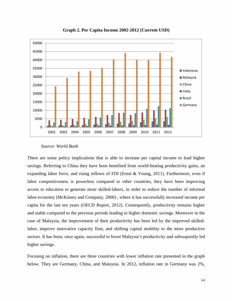
64
Graph 2. Per Capita Income 2002-2012 (Current USD)
Source: World Bank
There are some policy implications that is able to increase per capital income to lead higher
savings. Referring to China they have been benefited from world-beating productivity gains, an
expanding labor force, and rising inflows of FDI (Ernst & Young, 2011). Furthermore, even if
labor competitiveness is powerless compared to other countries, they have been improving
access to education to generate more skilled-labors, in order to reduce the number of informal
labor-economy (McKinsey and Company, 2006) , where it has successfully increased income per
capita for the last ten years (OECD Report, 2012). Consequently, productivity remains higher
and stable compared to the previous periods leading to higher domestic savings. Moreover in the
case of Malaysia, the improvement of their productivity has been led by the improved skilled-
labor, improve innovative capacity firm, and shifting capital mobility to the more productive
sectors. It has been, once again, successful to boost Malaysia‟s productivity and subsequently led
higher savings.
Focusing on inflation, there are three countries with lower inflation rate presented in the graph
below. They are Germany, China, and Malaysia. In 2012, inflation rate in Germany was 2%,
0
5000
10000
15000
20000
25000
30000
35000
40000
45000
50000
2002 2003 2004 2005 2006 2007 2008 2009 2010 2011 2012
Indonesia
Malaysia
China
India
Brazil
Germany

65
while China was 2.6%, and Malaysia was 1.6%. At the same level of income, people would save
more when inflation is relatively lower as they could spend less and save more. There are
distinctive steps in terms of how each country controls the inflation to keep lower. Instruments in
monetary policy, fiscal policy, and physical controls are the core determinants of low rate of
inflation on the top three countries to control inflation. Low inflation leads higher proportion to
save as expenses to consume tends to be lower.
Graph 3. Inflation Rate (Consumer Prices Annual %)
Source: World Bank 2012
In the above mentioned countries, it is seen that Germany, China, and Malaysia expense more for
their consumption. Nevertheless, as they can control the rate of inflation, then people can save
higher amount of money compared to those countries with high rate of inflation such as
Indonesia. Higher savings would lead higher allocation for investment to promote better
economic performance. Thus, what becomes the major concern is how to control core
determinants of savings themselves. Solow‟s (1965) growth model stated that developing
countries with lower capital stock could grow faster than developed countries through increasing
-2
0
2
4
6
8
10
12
14
16
2002 2003 2004 2005 2006 2007 2008 2009 2010 2011 2012
Indonesia
Malaysia
China
India
Brazil
Germany

66
savings and investment rates. The increasing role of capital market on growth tends to be a
substitute to the role of savings on growth.
4.2.2. Loan
From the output, it is seen that the total disaggregated-loan performs a significant and positive
effect on GDP. It expresses that 1% increase of loan would boost the growth by 0.054% with
95% level of confidence and has confronted some empirical findings. It confirms the research
conducted by Obamuyi, Edun, and Kayode (2010) expressing that bank lending on
manufacturing has a significant effect on manufacturing output in Nigeria. Moreover Takats and
Upper (2013) have found that bank credit has a significant effect in 39 countries even only after
the third and fourth year with small economic terms. Nevertheless, the result contradicts the
research conducted by Driscoll and Board (2003) expressing that loans have small, often
negative and statistically insignificant effects on output.
Graph 4. Total of Loan Distribution, Indonesia 2002-2012
Source: Bank Indonesia 2012
From the above graph, it is seen that Indonesia remains the lowest position in terms on domestic
credit (loan) to GDP ratio. As the result suggested that loan has a positive and significant impact
on growth, thus Indonesia would have achieved higher growth if loan had been well-optimized.
0
5
10
15
20
25
2002 2003 2004 2005 2006 2007 2008 2009 2010 2011 2012

67
Theoretically, loan distribution is influenced by several determinants such as cost of loans
(lending rate) and the rate of non-performing loans. Form the table below, Indonesia places the
second highest lending rate compared to Malaysia, China, India, and Brazil. Some empirical
findings has stated that lending rate has a negative and significant effect on loan distribution
(Castro and Santos, 2010). Thus it may explain that the relatively low distribution of loan
Indonesia has been led by the high cost of loan.
Graph 5. Lending Rates 2002-2012 (%)
Source: World Bank 2012
Furthermore, non-performing loans (NPL) in banking sectors are also the primary determinant in
terms of the volume of loan distribution. Tracey (2011) suggested that in making lending
decision, banks are assumed to react differently to NPL ratios above or below a threshold, with
NPLs above the threshold having an adverse effect on lending. Moreover, Hou and Dickinson
(2007) suggested that banks will reduce their loans supply at greater levels on NPLs/Loans ratio.
From the graph below, China is relatively successful in managing banking sector as indicated by
the lowest NPL to gross credit ratio that tends to decrease for the last 10 years.
0.0
10.0
20.0
30.0
40.0
50.0
60.0
70.0
80.0
2002 2003 2004 2005 2006 2007 2008 2009 2010 2011 2012
Indonesia
Malaysia
China
India
Brazil

68
Graph 6. NPL on Gross Credit Ratio 2002 – 2012 (%)
4.2.2.1. Loan for Investment
As presented in the output, it is seen that loan for investment has a significant and negative effect
on growth in the current year. It shows that 1% increase of loan for investment would be slowing
down the growth by 0.047%. Nevertheless, loan for investment performs positive effect on
growth in the lag 1 year indicating 1% increase of loan for investment would accelerate the
growth by 0.0008%, but is relatively insignificant. The negative finding contradicts both theory
and some empirical research expressing that funding of entrepreneurs (loans) would stimulate
more productivity and is subsequently supported by McKinnon (1973), Shaw (1973), Fry (1988),
and King and Levine (1993) by suggesting the above postulation about the significance of banks
to the performance of the economy. In the other cases, Cappiello, Kadareja, Sorensen, and
Protopapa (2010) found that the changes of credit supply in euro area, both in terms of values
and credit standards, have a positive and statistically significant effect on GDP. Interestingly, the
insignificant effect of loan for investment on growth confirmed some empirical findings such as
neither Driscoll (2004) nor Ashcraft (2006) found compelling facts for causal relationship
between credit supply and real output for the US case. Other findings by Takats and Upper
0
5
10
15
20
25
30
2002 2003 2004 2005 2006 2007 2008 2009 2010 2011 2012
Indonesia
Malaysia
China
India
Brazil
Germany

69
(2013) expressed that bank lending, to the private sector, is essentially uncorrelated to economic
performance after crises that were preceded by credit booms.
Focusing on the specified sector, loan for investment for the current year is significant on growth
for industry and trade with the 90% level of significance indicating that 1% increase of loan for
investment allocated for the respective sectors, would be slowing down the growth by 0.082%
for industry (manufacturing) and 0.109% for trade (including hotel and restaurant). Furthermore,
the positive and significant effect occurs on electricity (gas and water) showing 1% increase of
loan for investment would accelerate growth by 0.111% with 99% level of significance, while
the negative significant role is seen on construction (and building) sector where the growth
would be slowing down by 0.155% led by the increase of loan for investment by 1% with 99%
level of significance. In the other hand, loan for investment for the lag 1 year is significant on
industry (manufacturing) and transportation (and communication) suggesting 1% increase of
loan for investment for the respective sectors would be slowing down growth on industry by
0.137% and accelerating growth on transportation sector by 0.403% both with 99% level of
significance. Additionally, significant and negative effects are also seen on electricity and
services sectors implying 1% increase of loan for investment would be slowing down the growth
by 0.064% on electricity and 0.098% on services, both with 95% level of significance.
4.2.2.2. Loan for Working Capital
Loan for working capital shows a positive and significant effect in the current year. It indicates
that 1% increase in loan for working capital would accelerate the growth by 0.127% with 99%
level of significance. Nevertheless, the result tends to be different in the lag 1 year where it
provides negative and significant effect on growth indicating 1% increase in loan for working
capital would be slowing down growth by 0.047%.
Focusing on the sector specific, significant effect with 99% level of confidence of loan for
working capital is seen in industry (manufacturing) and electricity (including gas and water). It
expresses 1% increase of loan for working capital would be slowing down growth in industry
(manufacturing) sector by 0.18% and accelerating growth in electricity (including gas and water)
by 0.06%. Furthermore, loan for working capital would significantly accelerate the growth in
service sector by 0.049% with the 90% level of confidence. For the allocated loan for investment

70
in the lag 1 year, significant effect is seen on agriculture with 95% level of significance. It
indicates 1% increase in loan for working capital would be slowing down growth by 0.119%.
Besides, the positive and significant effect is seen on construction (building) and service
indicating 1% increase in loan for working capital would increase growth by 0.233% for
construction sector and 0.085% on service sector.
4.2.2.3. Loan for Consumption
It is seen that loan for consumption play a relatively major role in promoting better economic
performance as the result performs positive and significant effect on growth for both current and
lag 1 year. The result indicates that 1% of loan for consumption would be accelerating growth by
0.753% in the current year and by 0.304% in the lag 1 year. Higher contribution of loan for
investment in the current year explains that loan for consumption is relatively faster in giving
effect in the short-term compared to loan for investment and loan for working capital.
Lifecycle hypothesis by Modigliani and Brumberg (1954) establishes that households rely on
loans in order to smooth their consumption expenditure over the life cycle, according to the
present value of its future expected return. Variables of scale, such as economic activity or
disposable income, accordingly refl ect the ability of households to contract debt, since the
expectation of higher levels of income, permitting a higher debt burden to be serviced, leads to
higher indebtedness. Higher expenditure on consumption is eventually accumulated with
investment, government spending, and next export leading to a certain rate of economic in the
current year.
4.2.3. Foreign Direct Investment
It is seen from the result that foreign direct investment (FDI) has a significant and positive effect
on GDP growth reflecting 1% increase of FDI would be accelerating growth by 0.018% in the
current year. Nevertheless, the effect tends to be insignificant in the lag 1 year even it remains
positive. It reflects 1% increase in FDI for the lag 1 year would be accelerating growth by
0.001%. It confirms some of the previous empirical findings such as Anwar and Nguyen (2010)
focusing on Vietnam case, the relationship FDI on growth tends to be positive and significant.
Moreover, the effect would be higher if the investment is addressed, mainly, to education and
training to improve the local qualification and generate more output in the long-run.

71
Focusing on the sector specific analysis in the current year, the effect of FDI is significant on the
growth of industry (manufacturing), electricity (including gas and water), construction
(building), and trade sectors with 99% level of confidence, service sector with 95% level of
significance, and agriculture sector by 90% level of significance. The result indicates that 1%
increase of the respective sectors would be accelerating growth of industry by 0.09%, electricity
by 0.029%, and service sector by 0.121% and be slowing down growth of agriculture sector by
0.02%, construction sector by 0.055%, and trade by 0.176%. Moreover, the result of sector-
specific tends to be dynamic in the lag1 year where significant effects occurs on agriculture,
trade, finance, and services sector with the 99% level of confidence and industry (manufacturing)
sector with 90% level of confidence. It indicates 1% increase in the respective sectors would be
accelerating growth by 0.038% on industry sector, 0.019% on financial sector, 0.067% on
service sector, and be slowing down growth by 0.017% on agriculture sector and 0.097% on
trade sector.
Total net inflows of FDI in Indonesia have been increasing for the last 7 years. Nevertheless
compared to China, Brazil, Germany, and India, inflow of FDI in Indonesia tends to be lower. It
is important to notice that magnitude attraction of intention to invest in Indonesia is the existing
huge natural resources. It indicates that net inflow of FDI should have been higher if it had been
supported by effective and efficient procedures and bureaucracy. Indonesia is still below
Philippine in terms of standardized of corporate governance 2012 (Asia Standard of Corporate
Governance, 2012). Batubara (2010) stated on his article that Indonesia suffers from the problem
of investment constraints. He expressed that those constraints are instable political condition,
weak-constitution up-holding, complicated procedures, and less-integrated performance in
Indonesia.

72
Graph 7. Net Inflows of FDI 2005-2012, BoP US$
Source: World Bank
Table 4. Number of Start-up Procedures to Register a Business 2005-2012
Countries 2005 2006 2007 2008 2009 2010 2011 2012
Indonesia 12 12 12 12 11 11 10 10
Malaysia 10 10 10 10 10 9 3 3
China 13 13 13 14 14 14 14 13
India 11 11 13 13 13 12 12 12
Brazil 17 15 16 16 14 13 13 13
Germany 9 9 9 9 9 9 9 9
Source: World Bank
0
50
100
150
200
250
300
2005 2006 2007 2008 2009 2010 2011 2012
Indonesia
Malaysia
China
India
Brazil
Germany

73
4.2.4. Domestic Direct Investment
The result shows that domestic direct investment (DDI) has a significant and negative effect on
GDP growth indicating 1% increase of DDI would be slowing down growth by 0.033%.
Nevertheless, the effect tends to be insignificant even it remains negative in the lag 1 year
indicating 1% increase of DDI would be slowing down growth by 0.012%. It contradicted
previous empirical findings such as Borenztein et al (1998), De Mello (1999), and Braunstein
and Epstein (2002) expressing that domestic investment has a positive and significant effect on
growth even its contribution is relatively weak compared to foreign direct investment.
Nevertheless, FDI is able to off-set the role of domestic investment.
Nevertheless, focusing on the sector-specific analysis in the current year, its positive and
significant appears in the specific sectors. It is seen that DDI has a significant effect on
electricity (gas and water), trade (hotel and restaurant), transportation (and communication),
service sectors with 99% level of confidence, construction (building) sector with 95% level of
confidence, and industry (manufacturing sector) with 90% level of confidence. It shows that 1%
increase of the respective sectors would be accelerating growth by 0.015% on industry
(manufacture) sector, 0.091% on construction (building sector), 0.101% on trade (hotel and
restaurant) sector, and be slowing down growth by 0.147% on electricity (including gas and
water), 0.483% on transportation (and communication) sector, and 0.051% on service sector.
Nevertheless, a different result is seen in the lag 1 year for the sector-specific where agriculture,
industry (manufacturing), electricity (gas and water), transportation sectors are significant in
99% level of confidence, trade (hotel and restaurant) and service sectors are significant in 95%
level of confidence. It suggests that 1% increase of DDI would be accelerating growth by
0.022% on agriculture sector, 0.016% on industry (manufacturing) sector, 0.069% on trade (hotel
and restaurant) sector and be slowing down growth by 0.0119% on electricity (including gas and
water) sector, 0.0436% on transportation (and communication) sector, and 0.036% on service
sector. Less contributions on DDI is suspected to be similar to what happened with the role of
FDI in Indonesia

74
4.2.5. School Enrollment Rate
Education is a primary factor related to empowering human capital as one of the growth
function. In this research, the quality of human capital is proxied by school enrollment rate for
senior high school14
. The research shows that school enrollment rate for SMA (senior high
school) gives a positive and significant effect on growth by 0.0542% with 99% level of
significance. It confirms some of the previous empirical research such as Kaasa and Parts (2008)
emphasizing the importance of several cross-effects of human and social capital on economic
development. At national level, education seems to work together with institutional trust and
political activity, while micro-level social capital indicators did not show any significant
interaction with human capital. At regional level, interaction of education with formal and
informal networks has effect on GDP per capita changes and growth rates. The result also
confirms a study by Fleisher, Li, and Zhao (2007) expressing that human capital has a positive
and significant effect on TFP growth in China.
Focusing on sector-specific, school enrollment rate of senior high school (SMA) performs
significant and positive role on industry (manufacturing) sector, transportation (and
communication sector), and financial sector. It indicates 1% percent increase of school
enrollment rate of the respective sectors would be accelerating growth by 0.097% on industry
(manufacturing) sector, 0.0567% on transportation (and communication) sector, and 0.0186% on
financial sector.
4.2.6. Population Growth
The result indicates the growing population of Indonesia leads a slowing down economic
performance for the last 10 years. It is seen that population has a significant and negative effect
on growth indicating 1% increase on population would be slowing down growth by 0.214%. The
result confirms the theory of Solow and Swan (2002) expressing that population growth
negatively and significantly correlated to economic growth. Solow suggested that the increasing
growth of population would lead the decrease of capital to labor ratio thus decreases the
economic growth.
14
SMA is chosen to overcome the problem of multicollinearity as previously set along with the school enrollment rate for SD, SMP, and PT (higher education)

75
Focusing on the sector-specific analysis, population has a negative in all sectors of economic
activities except agriculture. With 95% level of confidence, 1% increase of population would be
accelerating growth by 0.063%. The negative and significant effect appears on industry
(manufacturing sector) and transportation (and communication sector) with 90% level of
confidence. It indicates 1% increase of population would be slowing down growth by 0.032% on
industry (manufacturing) sector and 0.171% on transportation (and communication) sector.
Graph 8. Employment to Population Ratio 2002-2012 (%)
Source: World Bank 2012
4.2.7. Seasonal Effect
In this research, dummy variable is employed to observe whether seasonal effect has significant
contribution on growth. Interestingly, seasonal effect plays a significant and positive role in the
case of Indonesia from 2002-2012. With 99% level of significance, seasonal effect contributes
respectively 5.6% in the first quarter and 50.7% in the second quarter. Moreover, seasonal effect
contributes 2.1% in the third quarter with 90% level of significance.
0
10
20
30
40
50
60
70
80
2002 2003 2004 2005 2006 2007 2008 2009 2010 2011 2012
Indonesia
Malaysia
China
India
Brazil
Germany

76
4.3. Bidirectional Relationship Analysis
Unit root test is the requirement for bidirectional or causal relationship in time series. The first
step is to conduct stationarity test using Augmented Dicky Fuller Test for the respective
variables. If the data is stationary on level, thus the test can be run using Vector-Autoregressive
(VAR), otherwise Vector Error Correction Model (VECM) is preferable. Using Granger
Causality Test, it would be clearly seen whether those variables perform bidirectional long run
relationship during the period.
Table 5. ADF Test
Variables Level First Difference
gdp -0.433 -9.270 ***
fdi -1.552 -5.593 ***
ddi -1.232 -5.490 ***
savings -1.392 -6.877 ***
l_inv -1.465 -6.157 ***
l_wc -1.521 -6.418 ***
l_cons -1.971 -6.215 ***
loan -0.139 -7.807 ***
smasrc -0.996 -3.929 ***
pop -4.043 -9.072 ***
Source: Data Process on STATA (2012)
As presented by the table above, all of data for each variable is stationary at the first difference
level. Thus Vector Error Correction Model is employed to observe bidirectional relationship
between variables.
Table 6. Granger Causality Test with Vector Error Correction Model
Dep Indep Coefficients Constanta
gdp fdi 0.005 -0.011
fdi gdp 184.854 *** -2.024
gdp ddi 0.002 -0.011
ddi gdp 634.972 *** -6.903
gdp savings 0.011 0.465
savings gdp 86.961 *** -0.920
gdp l_inv 0.011 0.432
l_inv gdp 91.725 *** -0.976

77
gdp l_wc 0.012 -0.011
l_wc gdp 85.920 *** -0.916
gdp l_cons 0.014 -0.011
l_cons gdp 71.632 *** -0.766
gdp loan 0.126 ** -0.014
loan gdp 7.959 *** -0.113
gdp smasrc 0.006 -0.010
smasrc gdp 165.022 *** -1.572
gdp pop 0.022 -0.010
pop gdp 46.299 *** -0.451
Source: Data Process STATA 12
From the paragraph above, it seen that most variables perform unidirectional relationship and
mostly from determinant of GDP growth. Only one variable performs bidirectional relationship
to GDP which is loan for consumption. The result indicates that 1% increase of loan for
consumption would increase the growth by 0.014%, while 1% increase of GDP growth would
increase loan for consumption by 0.126%. Focusing on unidirectional relationship, FDI does not
give a significant effect on growth while 1% increase on growth would surprisingly increase FDI
by 185%. It indicates that growth remain the core attraction for inviting more inflow of foreign
capital. Moreover, the same thing happens on DDI where there is no bidirectional relationship.
DDI does not significantly lead growth while 1% increase on growth would amazingly increase
DDI by 635%. The result confirms the increasing trend of DDI for the last 5 years. In the other
hand, unidirectional relationship also occurs in terms of savings and GDP where only 1%
increase on GDP would significantly increase savings by 87%. The same phenomenon is also
seen on loan for investment, loan for working capital, and total loan where 1% increase on GDP
growth would increase loan for investment by 92%, loan for working capital by 86%, and total
loan by 7.9%. Subsequently, unidirectional relationship also appears on school enrollment rate
(smascr) and population growth, where only 1% increase on growth would significantly increase
school enrollment rate by 165% and population by 46%. These findings express how growth
plays important role on some of growth‟s determinant itself in the long-run.
5. CONCLUSION
The paper has analyzed the role of savings and loans on gross domestic product of
Indonesia from 2002 to 2012, quarterly. Some empirical findings show that both savings and
78
loans have significant effects on GDP. It implies that savings and loans can be counted and
optimized to promote better economic performance of Indonesia in the future. Nevertheless,
some of other determinants suggest that FDI, indeed, has a positive and significant effect, while
DDI significantly and negatively influence GDP. Learning from the experience of Vietnam, the
allocations of investment should have been higher in education and training as human capital
remained the primary determinant of economic performance. The role of human capital as
proxied by school enrollment rate gives a positive and significant effect on economic growth. It
implies that human capital should have been the primary concern to start with in terms of
promoting better economic progress.
In the other hand, population growth suggests a negative and significant effect on GDP
while import perform positive and significant one. The negative contribution of population
confirms the Solow theory stating that higher population growth would slow down economic
growth as the decrease of capital to labor ratio. The overall results describes that the significant
effect remains not-optimized as the effects (reflected by the coefficients) are relatively small.
Thus, effective and efficient policies should have become the primary concern of the
government. The above findings have confirmed and contradicted with some of the previous
literatures. Further research and analysis in determinant of GDP growth is highly needed as the
comparison for the objectiveness of the current findings to provide better policy
recommendations in the future.

79
References
Abdi, Herve, “The Least Square,” The University of Texas Press, Dallas
Aghion, Philippe. Comin, Diego. Howitt, Peter., 2009, “When Does Domestic Saving Matter for
Economic Growth,” Brown University
Akaike, H. (1974). „A New Look at Statistical Model Identifications‟. IEEE Transitions on
Automatic Control, 19: 716-23.
Al-Foul, Bassam Abu, (2010), “The Causal Relationship between Savings and Economic
Growth: Some Evidence from MENA Countries,” The 30th
MENA Meeting_Atlanta.
Alfaro, Laura. (2003). “Foreign Direct Investment and Growth: Does the Sector Matter?”
Harvard Business School Press.
Alguacil, M., Cuadros, A., and Orts, V. (2004) “Does saving really matter for growth? Mexico
(1970-2000),” Journal of International Development. 16, Iss. 2, 281-290.
Allison, P.D. (1994), “Using Panel Data to Estimate the Effects of Events,” Sociological
Methods & Research 23: 174-199.
Anwar, Sajid. Nguyen, Lan Phi. (2010). “Foreign Direct Investment and Trade: The Case of
Vietnam," Asia Pacific Business Review.
Anyanwu CM (2000). Productivity in The Nigerian Manufacturing Industry, Paper Presented at
the 9th Annual Conference of Zonal Research Units, held at Abeokuta, June 12-16th.
Anyanwu SO (2009). “Analysis of Agricultural Gross Domestic Product (1960 – 2008) and
Implications For Agricultural Development in Nigeria” Intern. Journ of Agric and Rural
Development Vol.12, pp. 22-31.
Anyanwu SO, Ibekwe UC, Adesope OM (2010). “Agriculture Share of the Gross Domestic
Product and its Implications for Rural Development” Report and Opinion 2 (8): 26-31.
Anyanwu, SO. Offor, US. Adescope, OM. Ibekwe, UC. 2013. “Structure and Growth of the
Gross Domestic Product (1960-2008): Implications for small-scale enterprise in
Nigeria.” Global Advanced Research Journal of Management and Business Studies
(ISSN: 2315-5086) Vol. 2(6) pp. 342-348

80
Arcand, J.-L. 2000. Malnutrition and growth: The (efficiency) cost of hunger. Draft paper for
Agricultural Sector in Economic Development Service, Food and Agriculture
Organization of the United Nations.
Ashcraft, A. (2006), "New evidence on the lending channel", Journal of Money, Credit and
Banking 38(3), pp. 751-76.
Attanasio, Orazio P., Lucio Picci and Antonello Scurco. 2000. “Saving, Growth and Investment:
A Macroeconomic Analysis Using a Panel of Countries.” The Review of Economics and
Statistics 82 (2): 182-211.
Baltagi, B. H. (2006). “Panel Data Methods,” Texas A&M University College Station.
Baltagi, B. H. and C. Kao (2000). “Nonstationary panels, cointegration in panels and dynamic
panels: A survey.” Advances in Econometrics 15, 7-51.
Baltagi, B.H. et Kao, C. (2000), “Nonstationary panels, cointegration in panels and dynamic
panels: a survey,” in Advances in Econometrics, 15, edited by B. Baltagi et C. Kao, pp.
7-51, Elsevier Science.
Banerjee, Abhijit, and Esther Duflo. 2005. “Growth Theory Through the Lens of Development
Economics.” In Handbook of Economic Growth. Philippe Aghion and Steven N. Durlauf, eds.
Vol. 1A, pp. 473-552. Amsterdam: North-Holland.
Baumol, W.J., Blackman, S.A.B., and Wolfe, E.N., (1991). “Productivity and American
Leadership: The Long View.” Cambridge: MIT Press.
Beckmann, Elisabeth. Hake, Mariya. Urvova, Jarmila. (2013). “Determinants of Households’
Savings in Central, Eastern, and Southeastern Europe.” European Economic Integration
Q3/13.
Betyak, Olga. (2012). “An Econometric Analysis of Determinants of Economic Growth in Crisis
Countries of European Union.” Institute of Graduate Studies and Research Press.
Bosworth, B., (1993).“Saving and Investment in a Global Economy.” Washington: Brookings
Institution.
Bruderl, Josef. (2005). “Panel Data Analysis.” University of Mannheim, March
Burgess, Stephen. (2011). “Measuring Financial Sector Output and Its Contribution to UK
GDP.” Bank‟s Conjunctional Assessment and Projections Divisions, Quarterly Bulletin
(Q3)
Butler, Marguerite A. King, Aaron A. (2004). “Phylogenetic Comparative Analysis: A modeling
Approach for Adaptive Evolution.” The American Naturalist, Vol 164. No.6.

81
Burnham, Kenneth P. Anderson, David R. “Multimodel Inference: Understanding AIC and BIC
in Model Selection.” Colorado Cooperative Fish and Wildlife Research, Sociological
Methods & Research, Vol.33
Brüderl, Josef, 2005, “Panel Data Analysis,” University of Mannheim Press.
Carroll, C.D., Overland, J. and Weil, D.N. (2000). “Saving and growth with habit formation.”
The American Economic Review, Vol.90, No.3, pp.341-355.
Carroll, C.D. Weil, D N. (1994), “Saving and growth, a reinterpretation,” Cornegie-Rochester
Conference Series on Public Policy 40 (1994) 133-192, North-Holland
Castro, Grabriela. Santos, Carlos. (2010). “Bank Interest Rates and Loan Determinants,” Banco
de Portugal, Economics and Research Department
Capiello, Lorenzo. Kadareja, Arjan. Sorensen, Christoffer Kok. Protopapa, Marco. (2010). “Do
bank loans and credit standard have an effect on output? A panel approach for the Euro
Area,” Working Paper Series, No. 1150, Euro System, European Central Bank.
Cesaratto, Sergio (1999). “Savings and economic growth in neoclassical theory.” Cambridge
Journal of Economics, 23, 771-793.
Claus, Iris. Haugh, David. Scobie, Grant. Tornquist, Jonas. (2002), “Saving and Growth in an
open economy,” Treasury Working Paper 01/32, Wellington, New Zealand.
Cook, T.D. DeMets D.L. (2007). “Introduction to Statistical Methods for Clinical Trials.”
Champman and Hall Texts in Statistical Science.
Deaton, A.S. and Paxson, C.H., (1992). “Saving, Growth, and Aging in Taiwan, mimeo,”
Princeton University.
Demetriades, P.O. Andrianove, S. (2004). “Finance and Growth: What We Know and What We
Need to Know?” in C. A. E. Goodhart (ed). Financial Development and Growth:
Explaining the Links, Basingstoke: Palgrave Macmillan.
Demetriades, P.O. Hussein, K. (1996),“Does Financial Development cause Economic Growth?
Time Series Evidence from 16 countries”, Journal of Development Economics, 51, 387-
411.
Diao, X., Hazell, P., Resnick, D., & Thurlow, J. (2007b). “The role of agriculture in
development: Implications for sub-Saharan Africa”. Research report 153. Washington,
DC: IFPRI.
Diggle, Peter J.; Patrick Heagerty, Kung-Yee Liang, Scott L. Zeger (2002). “Analysis of
Longitudinal Data.” Oxford Statistical Science Series.

82
Domer, E.D. (1946) “Capital Expansion, Rate of Growth, and Employment,” Econometric, 14,
137-147.
Drapper, M.R. Smith, H. (1998). “Applied Regression Analysis.” Wiley Series in Probability and
Statistics.
Dougherty, Christopher (2007). “Introduction to Econometrics.” Oxford University Press.
p. 194.
Driscoll, John C. (2004). “Does Bank Lending Affect Output? Evidence From The U.S. States.”
Journal of Monetary Economics, Elsevier, Vol. 51(3), pages 451-471, April.
Easterly, William and Ross Levine. 2001. “It’s Not Factor Accumulation: Stylized Facts and
Growth Models.” World Bank Economic Review 15: 177-219.
Finkel, S. (1995), “Causal Analysis with Panel Data.” Sage Press
Fleisher, Belton. Li, Haizheng. Zhao, Min Qiang (2007). “Human Capital, Economic Growth,
and Regional Inequality in China.” Discussion Paper No. 2703
Fox, John. (2002). “Time Series Regression and Generalized Least Square.” Appendix to An R
and S-Plus Companion to Applied Regression.
Fry, M. J. (1988) “Money, Interest and Banking in Economic Development” John Hopkins
University Press, London.
Ghirmay T. (2004) “Financial Development and Economic Growth in Sub-Saharan African
Countries: Evidence from Time Series Analysis” African Development Bank
Ghozali, Imam. 2009. “Aplikasi Analisis Multivariate Dengan Program SPSS.” Jakarta: Gema
Pertama.
Gujarati, D. N. (1995). Basic Econometrics. New York: McGraw Hill, Inc. 3rd Edition
Greene. (2010). “Models for Panel Data.” ebook publication-214-242
Hahn, L.A: (1920), Volkswirtschaftliche Theorie des Bankkredits, Tübingen 1920: J.C.B. Mohr
(Paul Siebeck); 2nd ed. 1924; 3rd rev. ed. 1930; Italian translation as Teoria economica
del credito, edited and introduced by Lapo Berti, Naples 1990: Edizioni Scientifiche
Italiane.
Hall, Robert E., and Jones, Charles I. 1999. “Why Do Some Countries Produce So Much More
Output Per Worker Than Others?” Quarterly Journal of Economics 114(1): 83-116.
Harrod, R. (1939) “An Essay in Dynamic Theory,” Economic Journal, 49, 14-33.

83
Halaby, C. (2004), “Panel Models in Sociological Research,” Annual Rev. of Sociology 30: 507-
544.
Hevia, Constantino. Loayza, Norman. (2011). “Saving and Growth in Egypt,” Policy Research
Working Paper, 5529, Macroeconomics and Growth Team, Development Research
Group, The World Bank
Hou, Yixin & Dickinson, David. (2007). “The Non-Performing Loans: Some Bank-level Evidences,
Research Conference on Safety and Efficiency of the Financial System, August.
Hsiao, C., (2003), “Analysis of Panel Data,” second edition, Cambridge Universirty Press.
Hurlin C. (2010). “Panel Data Econometrics.” University of Orleans Press
Hurlin, C. et Mignon, V. (2005), “Une synthèse des tests de racine unitaire sur données de
panel,” Economie et Prévision, 169-170-171, pp. 253-294
Hutcheson, G. D. (2011). “Ordinary Least-Squares Regression.” In L. Moutinho and G. D.
Hutcheson, The SAGE Dictionary of Quantitative Management Research. Pages 224-
228.
Johansen, S. and Juselius, K. (1990). “Maximum likelihood estimation and inference on
cointegration with application to the demand for money.” Oxford Bulletin of Economics
and Statistics, Vol.52, pp.169- 210.
Kaasa, Anneli. Parts, Eve. (2008), “Human Capital and Social Capital as Interacting Factors of
Economic Development: Evidence from Europe” UTARTU, Working Paper IAREG
WP2/04
King, R.G., & Levine, R. (1993a). “Finance and Growth: Schumpeter Might Be Right.” –
Quarterly Journal of Economics, 108, 717-738.
King, R. G. & Levine R. (1993b), "Finance, Entrepreneurship, and Growth: Theory and
Evidence”, Journal of Monetary Economics, 32: 513-542.
King, R. G. & Levine R. (1993c), "Financial Intermediation and Economic Development”, In:
Financial Intermediation in the Construction of Europe, Eds: C. Mayer and X. Vives,
London: Centre for Economic Policy Research: 156-189.
Laura, Rizzi. (2013). “Test of Heteroscedasticity.” Econometric Journal Press.
Lean, Hooi Hooi. Song Yingzhe. (2008)“Domestic Saving and Economic Growth in China,”
Asian Business and Economic Research Unit Discussion Paper 64, 2008, Monash
University.
84
Levine, R. Loayza, N. & Beck, T. (2000) “Financial Intermediation and Economic Growth:
Causes and Causality” Journal of Monetary Economics No 46, pp31-77
Lin, S.Y. (1992). “Malaysia: saving-investment gap, financing needs and capital market
development.” Malaysia Management Review. Vol.27, No.4, pp.26-53.
Liu, J.Q. and Guo, Z.F. (2002). “Positive analysis of causal relationship between saving rate and
economic growth in China’s economy.” Zhong Guo Ruan Ke Xue, Vol.2.
Mankiw, Gregory, David Romer and David Weil. 1992. “A Contribution to the Empirics of
Economic Growth.” The Quarterly Journal of Economics 107 (2): 407-437
Modigliani, F. e Brumberg, R. (1954), “Utility analysis and the consumption function: An
interpretation of cross-section data in Post-Keynesian Economics,” K. K. Kurihara, pp.
128-197.
Makin, J.H. (2006). “Does China save and invest too much?” Cato Journal, Vol.26 No.2, pp.307.
Mankiw, N. Gregory (1992): Macroeconomics Third Edition. New York: Worth Publishers Inc.
McKinnon R. (1973). “Money and Capital in Economic Development.” Washington: The
Brookings Institute.
McQuinn, Kieran. Whelan, Karl. (2006). “Solow (1965) as a Model of Cross-Country
Dynamics.” Central Bank and Financial Services Authority of Ireland, October 9.
Modigliani, F. and Cao, S.L. (2004). “The Chinese saving puzzle and the life-cycle hypothesis.”
Journal of Economic Literature, Vol.42, No.1, pp.145-170.
Morgan, S.L. and Winship, C. (2007). “Counterfactuals and Causal Inference: Methods and
Principles for Social Research.” Cambridge U.P.
Nachrowi D Nachrowi. (2006), “Ekonometrika, untuk Analisis Ekonomi dan Keuangan.” The First
Publication: Faculty of Economics and Business, University of Indonesia.
Nielsen, Heino Bohn. (2005). “Generalized Method of Moments (GMM) Estimation.” Econometrics
2 – Fall.
Noy, Ilan. Nualsri, Aekkanush. (2007). “What do Exogenous Shocks Tell Us about Growth
Theories?” Department of Economics, University of Hawaii.
Oluitan, Roseline (2010). “Bank Credit and Economic Growth: The Nigerian Experience.”
Economic Press.
O‟Meara B. C., Ané C., Sanderson M. J., Wainwright P. C. 2006. “Testing for different rates of
continuous trait evolution using likelihood.” Evolution 60:922-933.

85
Pesaran, M. H., Shin, Y., and Smith, R. (2001) “Bound Testing Approaches to the Analysis of
Level Relationships,” Journal of Applied Econometrics, 16, 289-326.
Posada, David. Buckley, Thomas R. (2004). “Model Selection and Model Averaging in
Phylogenetics: Adavantages of Akaike Information Criterion and Bayesian Approaches
Over Likelihood Ratio Tests.” Landcare Research, Private Bag 92170, Auckland, New
Zealand.
Park, Hun Myoung. (2008), “Univariate Analysis and Normality Test Using SAS, STATA, and
SPSS.” Working Paper. The University Information Technology Services (UITS) Center
for Statistical and Mathematical Computing, Indiana University.
Ramsey, F. P. (1928). “A mathematical theory of saving.” The Economic Journal 38: 543-559.
Reinert, Gesine. (2010). “Time Series.” Hillary Term.
Roodman, David. (2009). “How to do xtabond2: An introduction to difference and system GMM
in STATA.” Center for Global Development, Washington, DC. The STATA Journal 9,
Number 1, pp. 86-136
Singer, J., and J. Willett (2003), “Applied Longitudinal Data Analysis,” Oxford Press
Solow, R.M. (1956) “A Contribution to the Theory of Economic Growth,” Quarterly Journal of
Economics, 70, 65-94.
Saltz, I.S. (1999) “An Examination of the Causal Relationship between Savings and Growth in
the Third World,” Journal of Economics and Finance, 23, 90-98.
Schumpeter, J. (1911), “Theorie der wirtschaftlichen Entwicklung,” Munich and Leipzig:
Duncker & Humblot. 2nd revised ed. 1926.
Schumpeter, J.A. (1917-18), “Das Sozialprodukt und die Rechenpfennige: Glossen und Beiträge
zur Geldtheorie von heute“, Archiv für Sozialwissenschaft und Sozialpolitik, 44: 627-
715; Engl. transl. by A. Marget, “Money and the Social Product“, International Economic
Papers, 6, 1956: 148-211.
Schumpeter, J.A. (1931), “The Theory of the Business Cycle“, Keizaigaku-Ronshu – The Journal
of Economics, 4: 1-32. 29
Schumpeter, J.A. (1939), “Business Cycles: A Theoretical, Historical and Statistical Analysis of
the Capitalist Process,” 2 vols., New York: McGraw-Hill.
Seren, Maria Jesus Freire. (2001). “Human Capital Accumulation and Economic Growth.”
Universidade de Vigo, Investigaciones Economicas. Vol XXV (3), 585602.

86
Shaw, E. S. (1973). “Financial Deepening in Economic Development.” Oxford University Press,
New York.
Shan J. & Jianhong Q. (2006) “Does Financial Development lead Economic Growth? The case
of China”. Annals of Economics and Finance 1 pp 231 – 250.
Singh, T. (2009) “Does domestic saving cause economic growth? A time-series evidence from
India,” Journal of Policy Modeling, doi:10.1016/j.jpolmod.2009.08.008,
Sinha, D. and Sinha, T. (1998) “Cart before the Horse? The Saving-Growth Nexus in Mexico,”
Economics Letters, 61,43-47.
Swan, T. W. (1956). “Economic growth and capital accumulation.” Economic Record 32: 334-
361.
Swiston A. (2008) “A US Financial Conditions Index: Putting Credit where Credit is Due” IMF
Working Paper, June.
Schwarz, Gideon. 1978. “Estimating the Dimension of a Model.” Annals of Statistics 6:461-4.
Takats, Elod. Upper, Christian. (2013). “Credit and Growth After Financial Crisis.” Monetary
and Economic Development, BIS Working Papers No. 416.
Tang T. C. (2003) “Directions of Bank lending and Malaysian Economic Development: An
Empirical Study” International Journal of Management, 20, 3, pp 342
Tang, Sumei. Selvanathan, E.A., Selvanathan, S. (2008) “Foreign Direct Investment, Domestic
Investment, and Economic Growth in China,” A Time Series Analysis, Research Paper
No. 2008/19. World Nations University.
Tracey, Mark. (2011). “The Impact of Non-Performing Loans on Loan Growth: an Econometric
Case Study of Jamaica and Trinidad and Tobago” IMF Journal.
Welch, F. (1970) "Education in Production," Journal of Economics of Political Economy, 78,
pp. 35-59.
Wooldridge J.M., (2001), “Econometric Analysis of Cross Section and Panel Data”, The MIT
Press.
Wooldridge, J. (2003), “Introductory Econometrics: A Modern Approach”. Thomson. Chap. 13,
14.
Wooldridge, J. (2002), “Econometric Analysis of Cross Section and Panel Data,” MIT Press.

87
Appendix
Model 1 PLS

88
Model 1 FE

89
Model 1 GMM Difference

90
Model 1 GMM System

91
Model 2 PLS

92
Model 2 FE

93
Model 2 GMM Difference
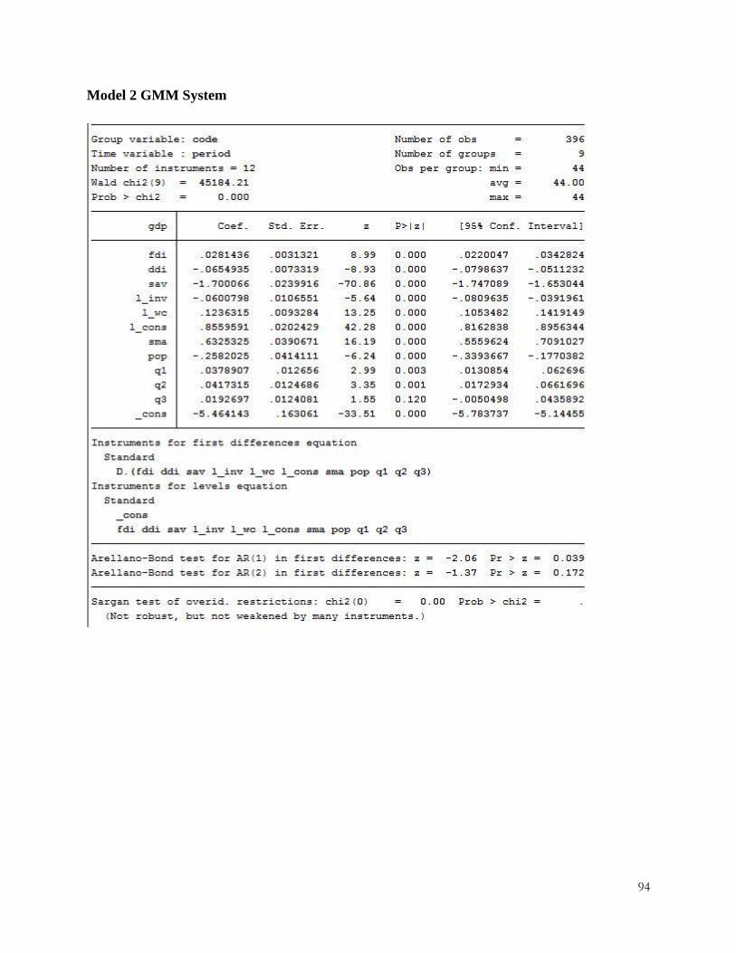
94
Model 2 GMM System

95
Model 3 PLS

96
Model 3 FE

97
Model 3 GMM Difference

98
Model 3 GMM System

99
Cross Section Specific Agriculture
Cross Section Specific Mining

100
Cross Section Specific Industry (Manufacturing)
Cross Section Specific Electricity, Gas, and Water

101
Cross Section Specific Construction and Building
Cross Section Specific Trade, Hotel, and Restaurant

102
Cross Section Specific Transportation and Communication
Cross Section Specific Financial Services

103
Cross Section Specific Services

104
GDP – FDI
Vector error-correction model
Sample: 4 - 44 No. of obs = 41
AIC = -5.058536
Log likelihood = 112.7 HQIC = -4.921563
Det(Sigma_ml) = .000014 SBIC = -4.682386
Equation Parms RMSE R-sq chi2 P>chi2
----------------------------------------------------------------
D_changegdp 4 .021008 0.7382 104.3452 0.0000
D_changefdi 4 .202155 0.2951 15.489 0.0038
----------------------------------------------------------------
------------------------------------------------------------------------------
| Coef. Std. Err. z P>|z| [95% Conf. Interval]
-------------+----------------------------------------------------------------
D_changegdp |
_ce1 |
L1. | -1.941735 .2638779 -7.36 0.000 -2.458926 -1.424543
|
changegdp |
LD. | .4189007 .1615414 2.59 0.010 .1022854 .7355161
|
changefdi |
LD. | .0069761 .0150425 0.46 0.643 -.0225066 .0364588
|
_cons | -.0023883 .0032863 -0.73 0.467 -.0088294 .0040528
-------------+----------------------------------------------------------------
D_changefdi |

105
_ce1 |
L1. | -3.390805 2.5392 -1.34 0.182 -8.367544 1.585935
|
changegdp |
LD. | .1856114 1.554453 0.12 0.905 -2.861061 3.232284
|
changefdi |
LD. | -.4628117 .1447482 -3.20 0.001 -.746513 -.1791104
|
_cons | .0013676 .0316232 0.04 0.966 -.0606128 .063348
------------------------------------------------------------------------------
Cointegrating equations
Equation Parms chi2 P>chi2
-------------------------------------------
_ce1 1 .1927719 0.6606
-------------------------------------------
Identification: beta is exactly identified
Johansen normalization restriction imposed
------------------------------------------------------------------------------
beta | Coef. Std. Err. z P>|z| [95% Conf. Interval]
-------------+----------------------------------------------------------------
_ce1 |
changegdp | 1 . . . . .
changefdi | .0054097 .0123211 0.44 0.661 -.0187393 .0295587
_cons | -.0109487 . . . . .
------------------------------------------------------------------------------

106
FDI – GDP
Vector error-correction model
Sample: 4 - 44 No. of obs = 41
AIC = -5.058536
Log likelihood = 112.7 HQIC = -4.921563
Det(Sigma_ml) = .000014 SBIC = -4.682386
Equation Parms RMSE R-sq chi2 P>chi2
----------------------------------------------------------------
D_changefdi 4 .202155 0.2951 15.489 0.0038
D_changegdp 4 .021008 0.7382 104.3452 0.0000
----------------------------------------------------------------
------------------------------------------------------------------------------
| Coef. Std. Err. z P>|z| [95% Conf. Interval]
-------------+----------------------------------------------------------------
D_changefdi |
_ce1 |
L1. | -.0183432 .0137363 -1.34 0.182 -.0452658 .0085794
|
changefdi |
LD. | -.4628117 .1447482 -3.20 0.001 -.746513 -.1791104
|
changegdp |
LD. | .1856114 1.554453 0.12 0.905 -2.861061 3.232284
|
_cons | .0013676 .0316232 0.04 0.966 -.0606128 .063348
-------------+----------------------------------------------------------------
D_changegdp |

107
_ce1 |
L1. | -.0105042 .0014275 -7.36 0.000 -.013302 -.0077063
|
changefdi |
LD. | .0069761 .0150425 0.46 0.643 -.0225066 .0364588
|
changegdp |
LD. | .4189007 .1615414 2.59 0.010 .1022854 .7355161
|
_cons | -.0023883 .0032863 -0.73 0.467 -.0088294 .0040528
------------------------------------------------------------------------------
Cointegrating equations
Equation Parms chi2 P>chi2
-------------------------------------------
_ce1 1 62.70756 0.0000
-------------------------------------------
Identification: beta is exactly identified
Johansen normalization restriction imposed
------------------------------------------------------------------------------
beta | Coef. Std. Err. z P>|z| [95% Conf. Interval]
-------------+----------------------------------------------------------------
_ce1 |
changefdi | 1 . . . . .
changegdp | 184.8535 23.3436 7.92 0.000 139.1009 230.6061
_cons | -2.0239 . . . . .
------------------------------------------------------------------------------

108
GDP – DDI
Vector error-correction model
Sample: 4 - 44 No. of obs = 41
AIC = -4.902722
Log likelihood = 109.5058 HQIC = -4.765749
Det(Sigma_ml) = .0000164 SBIC = -4.526572
Equation Parms RMSE R-sq chi2 P>chi2
----------------------------------------------------------------
D_changegdp 4 .02087 0.7417 106.2215 0.0000
D_changeddi 4 .221288 0.3215 17.53601 0.0015
----------------------------------------------------------------
------------------------------------------------------------------------------
| Coef. Std. Err. z P>|z| [95% Conf. Interval]
-------------+----------------------------------------------------------------
D_changegdp |
_ce1 |
L1. | -1.969662 .2662412 -7.40 0.000 -2.491485 -1.447839
|
changegdp |
LD. | .4311273 .1631203 2.64 0.008 .1114173 .7508372
|
changeddi |
LD. | .0001788 .0137651 0.01 0.990 -.0268004 .0271579
|
_cons | -.0025957 .0032663 -0.79 0.427 -.0089976 .0038062
-------------+----------------------------------------------------------------
D_changeddi |

109
_ce1 |
L1. | -4.582676 2.822979 -1.62 0.105 -10.11561 .9502617
|
changegdp |
LD. | .4955647 1.729579 0.29 0.774 -2.894347 3.885477
|
changeddi |
LD. | -.4820304 .1459527 -3.30 0.001 -.7680925 -.1959683
|
_cons | .0011157 .0346332 0.03 0.974 -.0667642 .0689955
------------------------------------------------------------------------------
Cointegrating equations
Equation Parms chi2 P>chi2
-------------------------------------------
_ce1 1 .0229742 0.8795
-------------------------------------------
Identification: beta is exactly identified
Johansen normalization restriction imposed
------------------------------------------------------------------------------
beta | Coef. Std. Err. z P>|z| [95% Conf. Interval]
-------------+----------------------------------------------------------------
_ce1 |
changegdp | 1 . . . . .
changeddi | .0015749 .0103902 0.15 0.880 -.0187896 .0219394
_cons | -.0108712 . . . . .

110
DDI – GDP
Vector error-correction model
Sample: 4 - 44 No. of obs = 41
AIC = -4.902722
Log likelihood = 109.5058 HQIC = -4.765749
Det(Sigma_ml) = .0000164 SBIC = -4.526572
Equation Parms RMSE R-sq chi2 P>chi2
----------------------------------------------------------------
D_changeddi 4 .221288 0.3215 17.53601 0.0015
D_changegdp 4 .02087 0.7417 106.2215 0.0000
----------------------------------------------------------------
------------------------------------------------------------------------------
| Coef. Std. Err. z P>|z| [95% Conf. Interval]
-------------+----------------------------------------------------------------
D_changeddi |
_ce1 |
L1. | -.0072171 .0044458 -1.62 0.105 -.0159308 .0014965
|
changeddi |
LD. | -.4820304 .1459527 -3.30 0.001 -.7680925 -.1959683
|
changegdp |
LD. | .4955647 1.729579 0.29 0.774 -2.894347 3.885477
|
_cons | .0011157 .0346332 0.03 0.974 -.0667642 .0689955
-------------+----------------------------------------------------------------
D_changegdp |

111
_ce1 |
L1. | -.003102 .0004193 -7.40 0.000 -.0039238 -.0022802
|
changeddi |
LD. | .0001788 .0137651 0.01 0.990 -.0268004 .0271579
|
changegdp |
LD. | .4311273 .1631203 2.64 0.008 .1114173 .7508372
|
_cons | -.0025957 .0032663 -0.79 0.427 -.0089976 .0038062
------------------------------------------------------------------------------
Cointegrating equations
Equation Parms chi2 P>chi2
-------------------------------------------
_ce1 1 66.63067 0.0000
-------------------------------------------
Identification: beta is exactly identified
Johansen normalization restriction imposed
------------------------------------------------------------------------------
beta | Coef. Std. Err. z P>|z| [95% Conf. Interval]
-------------+----------------------------------------------------------------
_ce1 |
changeddi | 1 . . . . .
changegdp | 634.9719 77.78886 8.16 0.000 482.5085 787.4352
_cons | -6.902893 . . . . .
------------------------------------------------------------------------------

112
GDP – Savings
Vector error-correction model
Sample: 4 - 44 No. of obs = 41
AIC = -5.14197
Log likelihood = 114.4104 HQIC = -5.004997
Det(Sigma_ml) = .0000129 SBIC = -4.76582
Equation Parms RMSE R-sq chi2 P>chi2
----------------------------------------------------------------
D_changegdp 4 .021173 0.7341 102.1509 0.0000
D_changesavings 4 .194033 0.3047 16.21421 0.0027
----------------------------------------------------------------
---------------------------------------------------------------------------------
| Coef. Std. Err. z P>|z| [95% Conf. Interval]
----------------+----------------------------------------------------------------
D_changegdp |
_ce1 |
L1. | -1.949029 .2585554 -7.54 0.000 -2.455788 -1.442269
|
changegdp |
LD. | .4261697 .1568556 2.72 0.007 .1187383 .733601
|
changesavings |
LD. | .0112289 .0150657 0.75 0.456 -.0182994 .0407572
|
_cons | -.0015696 .0033077 -0.47 0.635 -.0080526 .0049133
----------------+----------------------------------------------------------------
D_changesavings |

113
_ce1 |
L1. | -2.322859 2.369416 -0.98 0.327 -6.966829 2.321111
|
changegdp |
LD. | .2750338 1.437433 0.19 0.848 -2.542284 3.092352
|
changesavings |
LD. | -.5275054 .1380632 -3.82 0.000 -.7981044 -.2569065
|
_cons | .001317 .0303117 0.04 0.965 -.0580928 .0607269
---------------------------------------------------------------------------------
Cointegrating equations
Equation Parms chi2 P>chi2
-------------------------------------------
_ce1 1 .5349679 0.4645
-------------------------------------------
Identification: beta is exactly identified
Johansen normalization restriction imposed
-------------------------------------------------------------------------------
beta | Coef. Std. Err. z P>|z| [95% Conf. Interval]
--------------+----------------------------------------------------------------
_ce1 |
changegdp | 1 . . . . .
changesavings | .0114994 .0157221 0.73 0.465 -.0193154 .0423141
_cons | -.010583 . . . . .
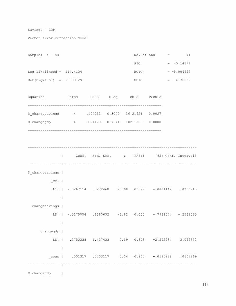
114
Savings – GDP
Vector error-correction model
Sample: 4 - 44 No. of obs = 41
AIC = -5.14197
Log likelihood = 114.4104 HQIC = -5.004997
Det(Sigma_ml) = .0000129 SBIC = -4.76582
Equation Parms RMSE R-sq chi2 P>chi2
----------------------------------------------------------------
D_changesavings 4 .194033 0.3047 16.21421 0.0027
D_changegdp 4 .021173 0.7341 102.1509 0.0000
----------------------------------------------------------------
---------------------------------------------------------------------------------
| Coef. Std. Err. z P>|z| [95% Conf. Interval]
----------------+----------------------------------------------------------------
D_changesavings |
_ce1 |
L1. | -.0267114 .0272468 -0.98 0.327 -.0801142 .0266913
|
changesavings |
LD. | -.5275054 .1380632 -3.82 0.000 -.7981044 -.2569065
|
changegdp |
LD. | .2750338 1.437433 0.19 0.848 -2.542284 3.092352
|
_cons | .001317 .0303117 0.04 0.965 -.0580928 .0607269
----------------+----------------------------------------------------------------
D_changegdp |

115
_ce1 |
L1. | -.0224126 .0029732 -7.54 0.000 -.02824 -.0165852
|
changesavings |
LD. | .0112289 .0150657 0.75 0.456 -.0182994 .0407572
|
changegdp |
LD. | .4261697 .1568556 2.72 0.007 .1187383 .733601
|
_cons | -.0015696 .0033077 -0.47 0.635 -.0080526 .0049133
---------------------------------------------------------------------------------
Cointegrating equations
Equation Parms chi2 P>chi2
-------------------------------------------
_ce1 1 65.6746 0.0000
-------------------------------------------
Identification: beta is exactly identified
Johansen normalization restriction imposed
-------------------------------------------------------------------------------
beta | Coef. Std. Err. z P>|z| [95% Conf. Interval]
--------------+----------------------------------------------------------------
_ce1 |
changesavings | 1 . . . . .
changegdp | 86.96122 10.73067 8.10 0.000 65.92949 107.9929
_cons | -.9203149 . . . . .
-------------------------------------------------------------------------------

116
GDP – l_inv
Vector error-correction model
Sample: 4 - 44 No. of obs = 41
AIC = -5.065858
Log likelihood = 112.8501 HQIC = -4.928885
Det(Sigma_ml) = .0000139 SBIC = -4.689708
Equation Parms RMSE R-sq chi2 P>chi2
----------------------------------------------------------------
D_changegdp 4 .021138 0.7350 102.6211 0.0000
D_changesl_inv 4 .200483 0.2872 14.90576 0.0049
----------------------------------------------------------------
--------------------------------------------------------------------------------
| Coef. Std. Err. z P>|z| [95% Conf. Interval]
---------------+----------------------------------------------------------------
D_changegdp |
_ce1 |
L1. | -1.937547 .2571593 -7.53 0.000 -2.44157 -1.433524
|
changegdp |
LD. | .4197111 .1568363 2.68 0.007 .1123177 .7271046
|
changesl_inv |
LD. | .0121139 .0147605 0.82 0.412 -.0168161 .041044
|
_cons | -.0011629 .0033013 -0.35 0.725 -.0076333 .0053075
---------------+----------------------------------------------------------------
D_changesl_inv |

117
_ce1 |
L1. | -2.898316 2.439078 -1.19 0.235 -7.678822 1.88219
|
changegdp |
LD. | .5712223 1.487545 0.38 0.701 -2.344312 3.486756
|
changesl_inv |
LD. | -.4997675 .1399988 -3.57 0.000 -.7741601 -.2253749
|
_cons | .0007774 .0313119 0.02 0.980 -.0605928 .0621476
--------------------------------------------------------------------------------
Cointegrating equations
Equation Parms chi2 P>chi2
-------------------------------------------
_ce1 1 .6184997 0.4316
-------------------------------------------
Identification: beta is exactly identified
Johansen normalization restriction imposed
------------------------------------------------------------------------------
beta | Coef. Std. Err. z P>|z| [95% Conf. Interval]
-------------+----------------------------------------------------------------
_ce1 |
changegdp | 1 . . . . .
changesl_inv | .0109021 .0138625 0.79 0.432 -.0162678 .038072
_cons | -.0106354 . . . . .
------------------------------------------------------------------------------

118
l_inv – GDP
Vector error-correction model
Sample: 4 - 44 No. of obs = 41
AIC = -5.065858
Log likelihood = 112.8501 HQIC = -4.928885
Det(Sigma_ml) = .0000139 SBIC = -4.689708
Equation Parms RMSE R-sq chi2 P>chi2
----------------------------------------------------------------
D_changesl_inv 4 .200483 0.2872 14.90576 0.0049
D_changegdp 4 .021138 0.7350 102.6211 0.0000
----------------------------------------------------------------
--------------------------------------------------------------------------------
| Coef. Std. Err. z P>|z| [95% Conf. Interval]
---------------+----------------------------------------------------------------
D_changesl_inv |
_ce1 |
L1. | -.0315977 .0265911 -1.19 0.235 -.0837152 .0205198
|
changesl_inv |
LD. | -.4997675 .1399988 -3.57 0.000 -.7741601 -.2253749
|
changegdp |
LD. | .5712223 1.487545 0.38 0.701 -2.344312 3.486756
|
_cons | .0007774 .0313119 0.02 0.980 -.0605928 .0621476
---------------+----------------------------------------------------------------
D_changegdp |

119
_ce1 |
L1. | -.0211233 .0028036 -7.53 0.000 -.0266182 -.0156284
|
changesl_inv |
LD. | .0121139 .0147605 0.82 0.412 -.0168161 .041044
|
changegdp |
LD. | .4197111 .1568363 2.68 0.007 .1123177 .7271046
|
_cons | -.0011629 .0033013 -0.35 0.725 -.0076333 .0053075
--------------------------------------------------------------------------------
Cointegrating equations
Equation Parms chi2 P>chi2
-------------------------------------------
_ce1 1 64.90293 0.0000
-------------------------------------------
Identification: beta is exactly identified
Johansen normalization restriction imposed
------------------------------------------------------------------------------
beta | Coef. Std. Err. z P>|z| [95% Conf. Interval]
-------------+----------------------------------------------------------------
_ce1 |
changesl_inv | 1 . . . . .
changegdp | 91.72549 11.38565 8.06 0.000 69.41002 114.041
_cons | -.9755401 . . . . .

120
GDP – l_wc
Vector error-correction model
Sample: 4 - 44 No. of obs = 41
AIC = -5.110438
Log likelihood = 113.764 HQIC = -4.973465
Det(Sigma_ml) = .0000133 SBIC = -4.734288
Equation Parms RMSE R-sq chi2 P>chi2
----------------------------------------------------------------
D_changegdp 4 .021076 0.7365 103.4366 0.0000
D_changesl_wc 4 .196731 0.3044 16.19272 0.0028
----------------------------------------------------------------
-------------------------------------------------------------------------------
| Coef. Std. Err. z P>|z| [95% Conf. Interval]
--------------+----------------------------------------------------------------
D_changegdp |
_ce1 |
L1. | -1.930612 .2538235 -7.61 0.000 -2.428097 -1.433127
|
changegdp |
LD. | .4154094 .154105 2.70 0.007 .1133692 .7174496
|
changesl_wc |
LD. | .0167791 .0147157 1.14 0.254 -.0120632 .0456215
|
_cons | -.0011895 .0032917 -0.36 0.718 -.0076412 .0052622
--------------+----------------------------------------------------------------
D_changesl_wc |

121
_ce1 |
L1. | -2.433875 2.369269 -1.03 0.304 -7.077558 2.209807
|
changegdp |
LD. | .7240228 1.438465 0.50 0.615 -2.095317 3.543363
|
changesl_wc |
LD. | -.5367386 .1373614 -3.91 0.000 -.8059621 -.2675152
|
_cons | .0009436 .0307262 0.03 0.976 -.0592786 .0611657
-------------------------------------------------------------------------------
Cointegrating equations
Equation Parms chi2 P>chi2
-------------------------------------------
_ce1 1 .6405111 0.4235
-------------------------------------------
Identification: beta is exactly identified
Johansen normalization restriction imposed
------------------------------------------------------------------------------
beta | Coef. Std. Err. z P>|z| [95% Conf. Interval]
-------------+----------------------------------------------------------------
_ce1 |
changegdp | 1 . . . . .
changesl_wc | .0116388 .0145426 0.80 0.424 -.0168643 .0401418
_cons | -.0106594 . . . . .
------------------------------------------------------------------------------

122
l_wc – GDP
Vector error-correction model
Sample: 4 - 44 No. of obs = 41
AIC = -5.110438
Log likelihood = 113.764 HQIC = -4.973465
Det(Sigma_ml) = .0000133 SBIC = -4.734288
Equation Parms RMSE R-sq chi2 P>chi2
----------------------------------------------------------------
D_changesl_wc 4 .196731 0.3044 16.19272 0.0028
D_changegdp 4 .021076 0.7365 103.4366 0.0000
----------------------------------------------------------------
-------------------------------------------------------------------------------
| Coef. Std. Err. z P>|z| [95% Conf. Interval]
--------------+----------------------------------------------------------------
D_changesl_wc |
_ce1 |
L1. | -.0283273 .0275754 -1.03 0.304 -.082374 .0257194
|
changesl_wc |
LD. | -.5367386 .1373614 -3.91 0.000 -.8059621 -.2675152
|
changegdp |
LD. | .7240228 1.438465 0.50 0.615 -2.095317 3.543363
|
_cons | .0009436 .0307262 0.03 0.976 -.0592786 .0611657
--------------+----------------------------------------------------------------
D_changegdp |
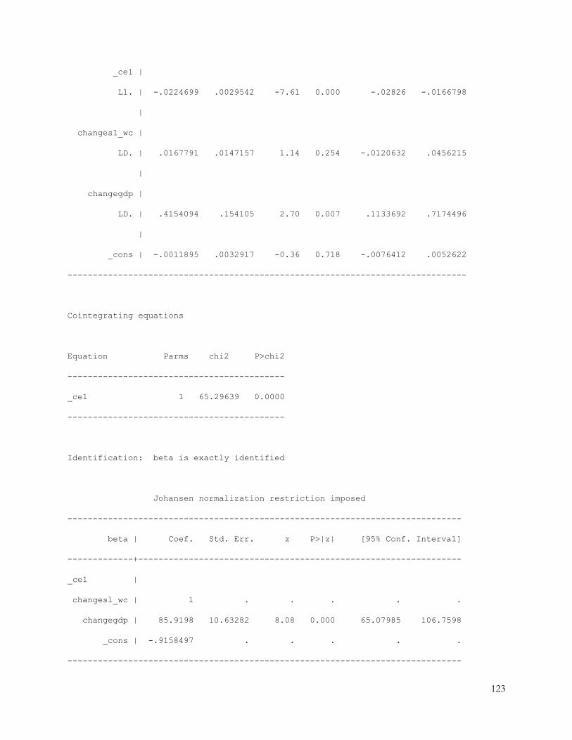
123
_ce1 |
L1. | -.0224699 .0029542 -7.61 0.000 -.02826 -.0166798
|
changesl_wc |
LD. | .0167791 .0147157 1.14 0.254 -.0120632 .0456215
|
changegdp |
LD. | .4154094 .154105 2.70 0.007 .1133692 .7174496
|
_cons | -.0011895 .0032917 -0.36 0.718 -.0076412 .0052622
-------------------------------------------------------------------------------
Cointegrating equations
Equation Parms chi2 P>chi2
-------------------------------------------
_ce1 1 65.29639 0.0000
-------------------------------------------
Identification: beta is exactly identified
Johansen normalization restriction imposed
------------------------------------------------------------------------------
beta | Coef. Std. Err. z P>|z| [95% Conf. Interval]
-------------+----------------------------------------------------------------
_ce1 |
changesl_wc | 1 . . . . .
changegdp | 85.9198 10.63282 8.08 0.000 65.07985 106.7598
_cons | -.9158497 . . . . .
------------------------------------------------------------------------------

124
.GDP – l_cons
Vector error-correction model
Sample: 4 - 44 No. of obs = 41
AIC = -5.061956
Log likelihood = 112.7701 HQIC = -4.924983
Det(Sigma_ml) = .000014 SBIC = -4.685806
Equation Parms RMSE R-sq chi2 P>chi2
----------------------------------------------------------------
D_changegdp 4 .021256 0.7320 101.0719 0.0000
D_changesl_cons 4 .20119 0.3184 17.28136 0.0017
----------------------------------------------------------------
---------------------------------------------------------------------------------
| Coef. Std. Err. z P>|z| [95% Conf. Interval]
----------------+----------------------------------------------------------------
D_changegdp |
_ce1 |
L1. | -1.922598 .259546 -7.41 0.000 -2.431299 -1.413898
|
changegdp |
LD. | .4153753 .1583613 2.62 0.009 .104993 .7257577
|
changesl_cons |
LD. | .0164578 .0144398 1.14 0.254 -.0118437 .0447592
|
_cons | -.0007249 .0033199 -0.22 0.827 -.0072318 .005782
----------------+----------------------------------------------------------------

125
D_changesl_cons |
_ce1 |
L1. | -3.367823 2.45665 -1.37 0.170 -8.182769 1.447124
|
changegdp |
LD. | .7517687 1.498918 0.50 0.616 -2.186057 3.689595
|
changesl_cons |
LD. | -.523565 .1366752 -3.83 0.000 -.7914434 -.2556865
|
_cons | .0004138 .0314236 0.01 0.989 -.0611753 .062003
---------------------------------------------------------------------------------
Cointegrating equations
Equation Parms chi2 P>chi2
-------------------------------------------
_ce1 1 1.060845 0.3030
-------------------------------------------
Identification: beta is exactly identified
Johansen normalization restriction imposed
-------------------------------------------------------------------------------
beta | Coef. Std. Err. z P>|z| [95% Conf. Interval]
--------------+----------------------------------------------------------------
_ce1 |
changegdp | 1 . . . . .
changesl_cons | .0139602 .0135539 1.03 0.303 -.012605 .0405255
_cons | -.0107002 . . . . .
-------------------------------------------------------------------------------

126
l_cons – GDP
Vector error-correction model
Sample: 4 - 44 No. of obs = 41
AIC = -5.061956
Log likelihood = 112.7701 HQIC = -4.924983
Det(Sigma_ml) = .000014 SBIC = -4.685806
Equation Parms RMSE R-sq chi2 P>chi2
----------------------------------------------------------------
D_changesl_cons 4 .20119 0.3184 17.28136 0.0017
D_changegdp 4 .021256 0.7320 101.0719 0.0000
----------------------------------------------------------------
---------------------------------------------------------------------------------
| Coef. Std. Err. z P>|z| [95% Conf. Interval]
----------------+----------------------------------------------------------------
D_changesl_cons |
_ce1 |
L1. | -.0470155 .0342953 -1.37 0.170 -.1142331 .0202021
|
changesl_cons |
LD. | -.523565 .1366752 -3.83 0.000 -.7914434 -.2556865
|
changegdp |
LD. | .7517687 1.498918 0.50 0.616 -2.186057 3.689595
|
_cons | .0004138 .0314236 0.01 0.989 -.0611753 .062003
----------------+----------------------------------------------------------------
D_changegdp |
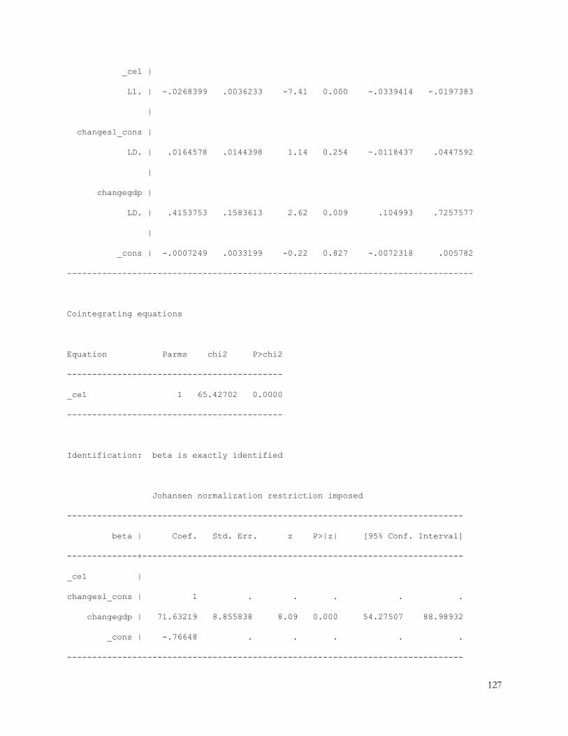
127
_ce1 |
L1. | -.0268399 .0036233 -7.41 0.000 -.0339414 -.0197383
|
changesl_cons |
LD. | .0164578 .0144398 1.14 0.254 -.0118437 .0447592
|
changegdp |
LD. | .4153753 .1583613 2.62 0.009 .104993 .7257577
|
_cons | -.0007249 .0033199 -0.22 0.827 -.0072318 .005782
---------------------------------------------------------------------------------
Cointegrating equations
Equation Parms chi2 P>chi2
-------------------------------------------
_ce1 1 65.42702 0.0000
-------------------------------------------
Identification: beta is exactly identified
Johansen normalization restriction imposed
-------------------------------------------------------------------------------
beta | Coef. Std. Err. z P>|z| [95% Conf. Interval]
--------------+----------------------------------------------------------------
_ce1 |
changesl_cons | 1 . . . . .
changegdp | 71.63219 8.855838 8.09 0.000 54.27507 88.98932
_cons | -.76648 . . . . .
-------------------------------------------------------------------------------

128
GDP – loan
Vector error-correction model
Sample: 4 - 44 No. of obs = 41
AIC = -9.630883
Log likelihood = 206.4331 HQIC = -9.49391
Det(Sigma_ml) = 1.45e-07 SBIC = -9.254733
Equation Parms RMSE R-sq chi2 P>chi2
----------------------------------------------------------------
D_changegdp 4 .01846 0.7979 146.0583 0.0000
D2_loan 4 .029806 0.8046 152.3591 0.0000
---------------------------------------------------------------
------------------------------------------------------------------------------
| Coef. Std. Err. z P>|z| [95% Conf. Interval]
-------------+----------------------------------------------------------------
D_changegdp |
_ce1 |
L1. | -2.677771 .3151426 -8.50 0.000 -3.295439 -2.060103
|
changegdp |
LD. | .9961851 .2741964 3.63 0.000 .45877 1.5336
|
loan |
LD2. | .3731123 .1160971 3.21 0.001 .1455662 .6006584
|
_cons | -.0004502 .0028848 -0.16 0.876 -.0061042 .0052038
-------------+----------------------------------------------------------------
D2_loan |
_ce1 |

129
L1. | 2.298235 .5088261 4.52 0.000 1.300954 3.295516
|
changegdp |
LD. | .1416035 .4427147 0.32 0.749 -.7261014 1.009308
|
loan |
LD2. | -.2242425 .1874492 -1.20 0.232 -.5916361 .1431512
|
_cons | -.0005245 .0046577 -0.11 0.910 -.0096534 .0086044
------------------------------------------------------------------------------
Cointegrating equations
Equation Parms chi2 P>chi2
-------------------------------------------
_ce1 1 6.438265 0.0112
-------------------------------------------
Identification: beta is exactly identified
Johansen normalization restriction imposed
------------------------------------------------------------------------------
beta | Coef. Std. Err. z P>|z| [95% Conf. Interval]
-------------+----------------------------------------------------------------
_ce1 |
changegdp | 1 . . . . .
|
loan |
D1. | .1256491 .0495193 2.54 0.011 .0285929 .2227052
|
_cons | -.0141944 . . . . .
------------------------------------------------------------------------------

130
loan – GDP
Vector error-correction model
Sample: 4 - 44 No. of obs = 41
AIC = -9.630883
Log likelihood = 206.4331 HQIC = -9.49391
Det(Sigma_ml) = 1.45e-07 SBIC = -9.254733
Equation Parms RMSE R-sq chi2 P>chi2
----------------------------------------------------------------
D2_loan 4 .029806 0.8046 152.3591 0.0000
D_changegdp 4 .01846 0.7979 146.0583 0.0000
----------------------------------------------------------------
------------------------------------------------------------------------------
| Coef. Std. Err. z P>|z| [95% Conf. Interval]
-------------+----------------------------------------------------------------
D2_loan |
_ce1 |
L1. | .288771 .0639335 4.52 0.000 .1634636 .4140784
|
loan |
LD2. | -.2242425 .1874492 -1.20 0.232 -.5916361 .1431512
|
changegdp |
LD. | .1416035 .4427147 0.32 0.749 -.7261014 1.009308
|
_cons | -.0005245 .0046577 -0.11 0.910 -.0096534 .0086044
-------------+----------------------------------------------------------------
D_changegdp |
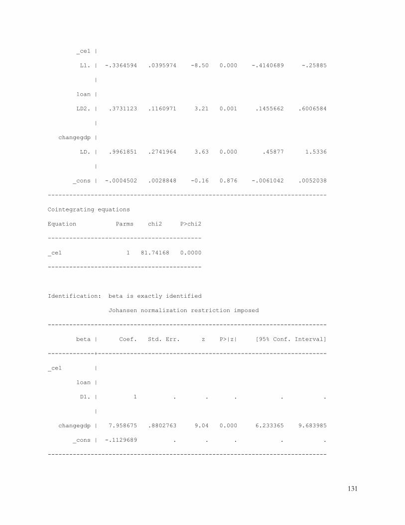
131
_ce1 |
L1. | -.3364594 .0395974 -8.50 0.000 -.4140689 -.25885
|
loan |
LD2. | .3731123 .1160971 3.21 0.001 .1455662 .6006584
|
changegdp |
LD. | .9961851 .2741964 3.63 0.000 .45877 1.5336
|
_cons | -.0004502 .0028848 -0.16 0.876 -.0061042 .0052038
------------------------------------------------------------------------------
Cointegrating equations
Equation Parms chi2 P>chi2
-------------------------------------------
_ce1 1 81.74168 0.0000
-------------------------------------------
Identification: beta is exactly identified
Johansen normalization restriction imposed
------------------------------------------------------------------------------
beta | Coef. Std. Err. z P>|z| [95% Conf. Interval]
-------------+----------------------------------------------------------------
_ce1 |
loan |
D1. | 1 . . . . .
|
changegdp | 7.958675 .8802763 9.04 0.000 6.233365 9.683985
_cons | -.1129689 . . . . .
------------------------------------------------------------------------------

132
GDP – smascr
Vector error-correction model
Sample: 4 - 44 No. of obs = 41
AIC = -7.076526
Log likelihood = 154.0688 HQIC = -6.939553
Det(Sigma_ml) = 1.87e-06 SBIC = -6.700376
Equation Parms RMSE R-sq chi2 P>chi2
----------------------------------------------------------------
D_changegdp 4 .020757 0.7444 107.7827 0.0000
D_changesmascr 4 .072939 0.0757 3.030595 0.5527
----------------------------------------------------------------
--------------------------------------------------------------------------------
| Coef. Std. Err. z P>|z| [95% Conf. Interval]
---------------+----------------------------------------------------------------
D_changegdp |
_ce1 |
L1. | -1.968231 .2471877 -7.96 0.000 -2.45271 -1.483752
|
changegdp |
LD. | .426571 .1501209 2.84 0.004 .1323395 .7208026
|
changesmascr |
LD. | .0050885 .0449957 0.11 0.910 -.0831014 .0932784
|
_cons | 3.98e-06 .0032442 0.00 0.999 -.0063546 .0063626
---------------+----------------------------------------------------------------
D_changesmascr |

133
_ce1 |
L1. | -.0193101 .8685875 -0.02 0.982 -1.72171 1.68309
|
changegdp |
LD. | -.0187983 .5275065 -0.04 0.972 -1.052692 1.015095
|
changesmascr |
LD. | -.2743332 .1581093 -1.74 0.083 -.5842218 .0355553
|
_cons | -.0004055 .0113999 -0.04 0.972 -.0227489 .0219379
--------------------------------------------------------------------------------
Cointegrating equations
Equation Parms chi2 P>chi2
-------------------------------------------
_ce1 1 .0454438 0.8312
-------------------------------------------
Identification: beta is exactly identified
Johansen normalization restriction imposed
------------------------------------------------------------------------------
beta | Coef. Std. Err. z P>|z| [95% Conf. Interval]
-------------+----------------------------------------------------------------
_ce1 |
changegdp | 1 . . . . .
changesmascr | .0060598 .0284263 0.21 0.831 -.0496548 .0617744
_cons | -.009525 . . . . .
------------------------------------------------------------------------------

134
Smascr – GDP
Vector error-correction model
Sample: 4 - 44 No. of obs = 41
AIC = -7.076526
Log likelihood = 154.0688 HQIC = -6.939553
Det(Sigma_ml) = 1.87e-06 SBIC = -6.700376
Equation Parms RMSE R-sq chi2 P>chi2
----------------------------------------------------------------
D_changesmascr 4 .072939 0.0757 3.030595 0.5527
D_changegdp 4 .020757 0.7444 107.7827 0.0000
----------------------------------------------------------------
--------------------------------------------------------------------------------
| Coef. Std. Err. z P>|z| [95% Conf. Interval]
---------------+----------------------------------------------------------------
D_changesmascr |
_ce1 |
L1. | -.000117 .0052635 -0.02 0.982 -.0104332 .0101992
|
changesmascr |
LD. | -.2743332 .1581093 -1.74 0.083 -.5842218 .0355553
|
changegdp |
LD. | -.0187983 .5275065 -0.04 0.972 -1.052692 1.015095
|
_cons | -.0004055 .0113999 -0.04 0.972 -.0227489 .0219379
---------------+----------------------------------------------------------------
D_changegdp |

135
_ce1 |
L1. | -.0119271 .0014979 -7.96 0.000 -.0148629 -.0089912
|
changesmascr |
LD. | .0050885 .0449957 0.11 0.910 -.0831014 .0932784
|
changegdp |
LD. | .426571 .1501209 2.84 0.004 .1323395 .7208026
|
_cons | 3.98e-06 .0032442 0.00 0.999 -.0063546 .0063626
--------------------------------------------------------------------------------
Cointegrating equations
Equation Parms chi2 P>chi2
-------------------------------------------
_ce1 1 63.43716 0.0000
-------------------------------------------
Identification: beta is exactly identified
Johansen normalization restriction imposed
------------------------------------------------------------------------------
beta | Coef. Std. Err. z P>|z| [95% Conf. Interval]
-------------+----------------------------------------------------------------
_ce1 |
changesmascr | 1 . . . . .
changegdp | 165.022 20.71906 7.96 0.000 124.4134 205.6307
_cons | -1.571827 . . . . .

136
GDP – Population
Vector error-correction model
Sample: 4 - 44 No. of obs = 41
AIC = -4.862461
Log likelihood = 108.6804 HQIC = -4.725488
Det(Sigma_ml) = .0000171 SBIC = -4.486311
Equation Parms RMSE R-sq chi2 P>chi2
----------------------------------------------------------------
D_changegdp 4 .020806 0.7433 107.1095 0.0000
D_changepop 4 .220809 0.4190 26.68585 0.0000
----------------------------------------------------------------
------------------------------------------------------------------------------
| Coef. Std. Err. z P>|z| [95% Conf. Interval]
-------------+----------------------------------------------------------------
D_changegdp |
_ce1 |
L1. | -1.910798 .2413138 -7.92 0.000 -2.383764 -1.437832
|
changegdp |
LD. | .3956499 .1475631 2.68 0.007 .1064315 .6848682
|
changepop |
LD. | .0286303 .0121558 2.36 0.019 .0048053 .0524552
|
_cons | -.0005636 .0032498 -0.17 0.862 -.0069332 .005806
-------------+----------------------------------------------------------------
D_changepop |

137
_ce1 |
L1. | -2.712167 2.561033 -1.06 0.290 -7.731698 2.307365
|
changegdp |
LD. | 1.827936 1.566068 1.17 0.243 -1.241501 4.897374
|
changepop |
LD. | -.5972903 .1290081 -4.63 0.000 -.8501415 -.344439
|
_cons | .0003971 .0344901 0.01 0.991 -.0672023 .0679965
------------------------------------------------------------------------------
Cointegrating equations
Equation Parms chi2 P>chi2
-------------------------------------------
_ce1 1 1.55018 0.2131
-------------------------------------------
Identification: beta is exactly identified
Johansen normalization restriction imposed
------------------------------------------------------------------------------
beta | Coef. Std. Err. z P>|z| [95% Conf. Interval]
-------------+----------------------------------------------------------------
_ce1 |
changegdp | 1 . . . . .
changepop | .0215989 .0173476 1.25 0.213 -.0124019 .0555997
_cons | -.0097373 . . . . .
------------------------------------------------------------------------------
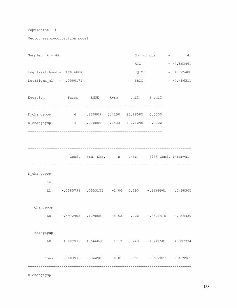
138
Population – GDP
Vector error-correction model
Sample: 4 - 44 No. of obs = 41
AIC = -4.862461
Log likelihood = 108.6804 HQIC = -4.725488
Det(Sigma_ml) = .0000171 SBIC = -4.486311
Equation Parms RMSE R-sq chi2 P>chi2
----------------------------------------------------------------
D_changepop 4 .220809 0.4190 26.68585 0.0000
D_changegdp 4 .020806 0.7433 107.1095 0.0000
----------------------------------------------------------------
------------------------------------------------------------------------------
| Coef. Std. Err. z P>|z| [95% Conf. Interval]
-------------+----------------------------------------------------------------
D_changepop |
_ce1 |
L1. | -.0585798 .0553155 -1.06 0.290 -.1669961 .0498365
|
changepop |
LD. | -.5972903 .1290081 -4.63 0.000 -.8501415 -.344439
|
changegdp |
LD. | 1.827936 1.566068 1.17 0.243 -1.241501 4.897374
|
_cons | .0003971 .0344901 0.01 0.991 -.0672023 .0679965
-------------+----------------------------------------------------------------
D_changegdp |

139
_ce1 |
L1. | -.0412711 .0052121 -7.92 0.000 -.0514867 -.0310556
|
changepop |
LD. | .0286303 .0121558 2.36 0.019 .0048053 .0524552
|
changegdp |
LD. | .3956499 .1475631 2.68 0.007 .1064315 .6848682
|
_cons | -.0005636 .0032498 -0.17 0.862 -.0069332 .005806
------------------------------------------------------------------------------
Cointegrating equations
Equation Parms chi2 P>chi2
-------------------------------------------
_ce1 1 62.13639 0.0000
-------------------------------------------
Identification: beta is exactly identified
Johansen normalization restriction imposed
------------------------------------------------------------------------------
beta | Coef. Std. Err. z P>|z| [95% Conf. Interval]
-------------+----------------------------------------------------------------
_ce1 |
changepop | 1 . . . . .
changegdp | 46.29866 5.873479 7.88 0.000 34.78686 57.81047
_cons | -.4508236 . . . . .
------------------------------------------------------------------------------

140