
The Company that You Keep: When to Buy a …...The Company that You Keep: When to Buy a...
55
The Company that You Keep: When to Buy a Competitor’s Keyword Woochoel Shin Duke University September 2009 Woochoel Shin is a PhD Candidate at the Fuqua School of Business, Duke University, Durham, NC 27708; Phone: 919-660-7627; Email: [email protected]. This research is a part of the author’s doctoral dissertation proposal. He thanks his dissertation committee: Preyas Desai (co-chair), Richard Staelin (co-chair), Kenneth Wilbur, and Huseyin Yildirim for their support and guidance.
Transcript of The Company that You Keep: When to Buy a …...The Company that You Keep: When to Buy a...
The Company that You Keep:
When to Buy a Competitor’s Keyword
Woochoel ShinDuke University
September 2009
Woochoel Shin is a PhD Candidate at the Fuqua School of Business, Duke University, Durham,NC 27708; Phone: 919-660-7627; Email: [email protected]. This research is a part of the author’sdoctoral dissertation proposal. He thanks his dissertation committee: Preyas Desai (co-chair),Richard Staelin (co-chair), Kenneth Wilbur, and Huseyin Yildirim for their support and guidance.

The Company that You Keep:
When to Buy a Competitor’s Keyword
Abstract
In search advertising, we observe different patterns of branded keyword purchase behaviorby the brand owner and its competitor. In particular, under a specific branded keyword,we may observe in the sponsored link, only the brand owner, only the competitor, both, orneither. In this paper, we aim to understand their strategies in a competitive environment.We first derive conditions for each purchase pattern to emerge as an equilibrium. On probingfurther the underlying incentives, we find that in some cases, the brand owner may buyits own keyword only to defend itself from the competitor’s threat. In contrast, we alsoidentify the case where the brand owner chooses to buy its own keyword and precludes thecompetitor from buying it. Our result also implies that both firms may be worse off byengaging in advertising, as in the prisoner’s dilemma case. Finally, we propose an analysison the impact of the insufficient advertising budget. If the budget is limited, both firms mayhave an incentive to hurt the competitor taking the higher slot, by increasing the bid amountand thus quickly exhausting the competitor’s budget. Additionally, the budget constraintmay make it less likely for each firm to buy the keyword in equilibrium.
Keywords: Search Advertising, Keyword Selection, Branded Keywords, RaisingRivals’ Cost, Game Theory.

1
1 Introduction
Type Gucci in Google’s search box. You will see Gucci taking the first slot of both sponsored
links and organic links. Now, type Dior. You will find only the organic link but not the
sponsored link of Dior. What about Camry? Toyota comes out in the sponsored section as
well as in the organic section. However, you will also observe some of its competitors listed
in the sponsored section: Chevy Malibu and Nissan Altima. Finally, try Harvard MBA. Do
you see Harvard Business School in the sponsored link? No. Only its competitors show up
there.1
Why does Gucci buy its own name, while Dior does not? Why do Toyota’s competitors
advertise under Toyota’s brand Camry, while Gucci’s or Dior’s competitors do not advertise
under Gucci or Dior? Why does Harvard let its competitors make use of its own brand
name? In this paper, we attempt to understand why we observe different patterns of branded
keyword purchase behavior. In particular, we investigate the purchase decision of the brand
owner and the competitors as well as their underlying incentives for the purchase or no
purchase decision. Further, we aim to provide a normative guideline in the selection of the
branded keyword.
Branded keywords have been proved to be effective in increasing the click-through rate
(Rutz and Bucklin 2007), and many advertisers use the branded keyword to collect more
relevant clicks to their sites. However, increasing the number of clicks is not the only objective
for the use of a branded keyword. An advertiser may also be concerned with the brand
awareness or the brand’s perceived quality. Thus, in this paper, we focus on the understudied
yet important aspect of the keyword search advertising: brand advertising, and investigate
how it affects the strategic decision of advertisers.
In this regard, we ask the following three questions: (1) When do we observe one purchase
pattern over another? (2) Why do brand owners buy their own branded keyword? (3) Why
1See Figure 1 for the screen captures. We have observed each example consistently showing the samepattern for more than a year.

2
do some firms forgo the opportunity to advertise their less known brand names under the
competitor’s well-known brand name?
To answer these questions, we develop a model of duopoly where two firms compete with
each other in a product market as well as in the search advertising market. Both offer a
vertically and horizontally differentiated product, and the brand owner provides the higher
quality product. The two firms also engage in search advertising to promote their brands.
Specifically, we describe the benefit of advertising using two well-documented phenomena:
the exposure effect and the contrast-assimilation effect. The exposure effect captures an
increase in the brand awareness or the brand’s perceived quality through exposure of the
brand’s advertisement. The contrast-assimilation effect refers to a positive or negative bias
associated with consumers seeing the two brand names simultaneously. Specifically, con-
sumers perceive brands that differ substantially in quality to be more different than they
actually are and similar brands to be more similar than they actually are.
Based on these two effects, our model answers the first question by providing an integrated
framework to define the condition for each pattern of purchase decision: (1) both firms
buying, (2) only the brand owner buying, (3) only the competitor buying, and (4) neither
buying. First, if the exposure effect is small, neither firm will buy, because they cannot
justify the cost of advertising. If the exposure effect is above a certain threshold, at least one
of them will buy. What matters now is the contrast-assimilation effect because firms consider
how they are viewed by the consumer when they are compared with their competitor. If there
is a large contrast effect, only the brand owner buys the keyword because the competitor
with an inferior product would be hurt by the contrast effect. If there is a large assimilation
effect, only the competitor is observed in equilibrium because now the brand owner would
be hurt by the assimilation effect. If neither effect is large, both firms choose to advertise
together because neither firm finds the effect of comparison too detrimental.
We also examine the strategic concerns of both firms in order to provide a deeper under-
standing of their incentives. First, we find that in some cases, the brand owner may purchase

3
its own branded keyword solely to defend itself from the competitor’s encroachment. This
happens when the exposure effect is somewhat weak and neither the contrast nor assimilation
effect is large. Because of the weak exposure, the brand owner would not buy the keyword if
its competitor does not buy. However, if the competitor buys the keyword, the brand owner
has an incentive to buy its own keyword because the brand owner is negatively affected in
the product market by letting the competitor advertise alone. This negative impact can be
reduced if the brand owner also purchases the keyword. Note however, the brand owner does
not succeed in driving out its competitor.
Our result also identifies the case where by purchasing its own keyword, the brand owner
succeeds in effectively precluding the competitor from buying the owner’s branded keyword.
We observe this pattern when both the exposure effect and the contrast effect are large.
In this case, though the competitor would prefer to advertise because of the large exposure
effect, the brand owner discourages this attempt by purchasing its own keyword. This
exclusion is possible because the large contrast effect makes the brand owner’s threat credible
and at the same time, it deprives of the competitor the incentive to match the brand owner’s
purchase decision. When the assimilation effect is large, we obtain the opposite result. The
competitor may discourage the brand owner’s attempt to utilize its own brand name. Even
though the brand owner would like to advertise without the competitor’s advertisement, it
would withdraw in the presence of the competitor, in fear of the loss due to assimilation.
Two firms, when purchasing the branded keyword, may expect to see an increase in their
profits. However, they are not always better off. Instead, for some intermediate values of the
contrast-assimilation effect (i.e., low contrast or low assimilation), we observe a prisoner’s
dilemma case where both firms are worse off by engaging in search advertising. This is
because when the comparative benefit (of a contrast or an assimilation) is not large, the
direct benefit dictates the profitability, but if both of them expect to get a direct benefit by
advertising together, these direct benefits are canceled out by each other.
Finally, we propose to investigate how the advertising incentives change if there is an

4
advertising budget constraint. For this, we first characterize the strategic interaction in the
bidding game. We start with the observation that in the context of the generalized second-
price auction format, the second slot winner can hurt the first slot winner by increasing the
advertising cost of the first slot winner. This increased cost coupled with the first firm’s
budget constraint can result in the first firm not always advertising. This allows the second
firm to appear in the first slot at times. This in turn benefits the second firm in the product
market competition. This interesting interaction between the two competitors is possible
because the search engine uses the second price auction rule.
We plan to investigate how the budget constraint changes the keyword purchase strategy
outlined above. First, we expect that the limited budget makes the purchase of the keyword
less attractive compared to the no purchase option and thus it becomes less likely to observe
both firms advertising. Second, we predict that the need for the defensive purchase by the
brand owner may be reduced because the competitor is less likely to buy and thus the threat
of the competitor is less severe. At the same time, preclusion may be more prevalent as firms
are affected more severely by the same amount of loss.
Our theoretical model is based on two well-established effects. In addition, these effects
are subjected to empirical investigation in the context of search advertising. We conducted an
experiment where we exposed participants to a search engine result page with different sets
of brands (brand owner only, competitor only, both, or neither) in the sponsored link section
of the page, and collected the consumers’ quality perceptions of each brand. We also varied
the quality difference between the brand owner and the competitor by using two different
competitor brand names. We found a significant exposure effect associated with competitor
advertisements. However, the exposure effect of the brand owner’s advertisement was not
significantly different from zero. In our experiment, because the brand owner was well-known
for its premium quality, it may have been hard to see any difference in quality perception by
a single advertisement exposure. The contrast effects were positive and significant in both
cases. We interpret this result as evidence of both competitors being far enough from the

5
brand owner. The sizes of the two competitor brands’ contrast effects were directionally
different but not significantly different. Thus, we empirically establish the existence of the
two effects (the exposure effect and the contrast-assimilation effect) in a search advertising
context.
We base our work on the search advertising literature. The literature in economics starts
with Edelman et al. (2007) and Varian (2007), both of which characterize the keyword
auction problem and offer solutions to this problem. Since then, there has been a series of
papers investigating the search engine’s mechanism design problem such as advertiser ranking
determination (Balachander and Kannan 2008, Desai and Shin 2006, Lahaie 2006), minimum
bids (Desai and Shin 2009, Liu et al. 2008), auction format (Yao and Mela 2009), and
payment scheme (Dellarocas and Viswanathan 2008). Another set of papers focuses on the
advertiser’s problems including bidding strategy (Katona and Sarvary 2008, Ghose and Yang
2009), keyword selection (Rutz and Bucklin 2007a), and performance measurement problem
(Rutz and Bucklin 2007b). There also have been attempts to link the search advertising
model to the consumer search model (Athey and Ellison 2008, Chen and He 2008, Jerath
et al. 2009) in explaining the equilibrium outcome of the keyword auction. Finally, Wilbur
and Zhu (2009) investigate the click-fraud problem.
We contribute to the search advertising literature in three regards. First, we go beyond
academia’s focus on the click-generating role of search advertising, and examine an increasing
interest of the industry, the brand-lifting role (Google and Media Screen 2008, Enquiro
Research and Google 2007). We model the brand advertising aspect of search advertising,
to our knowledge, for the first time. Second, in doing so, we investigate the link between the
search advertising market and the product market. Although one can easily think that the
advertising decision affects the product market outcome, the search advertising literature has
generally ignored the link between the search advertising market and the product market
competition.2 We specifically consider the impact of advertising decision on the product
2The exception is Xu et al. (2009), which explicitly linked the pricing decision in the product market tothe bidding decision in search advertising. Chen and He (2006) also consider product market competition

6
market outcome such as the equilibrium price and sales, by jointly modeling the product
market competition and the competition in search advertising. Finally, we focus on branded
keywords. We believe this is important because branded keywords will be used more in
consumer search as more firms try to link search advertising with other media advertising
(Online Publishers Association 2009). In addition, recent lawsuits between Google and
several advertisers on the use of trademark reflects an increasing interest in the issue (Helft
2009, Orey 2009). By analyzing the effect of using one’s own as well as the competitor’s
branded keywords, we offer insight to a practical problem in the field.
A second stream of research that we use is the literature on the contrast-assimilation
effect. Hovland et al. (1957) show a contrast effect and an assimilation effect in a social
communication context. They defined a latitude of acceptance, where assimilation occurs
with greater discrepancy from one’s position and contrast occurs with less discrepancy. In
a different context, Sherif et al. (1958) show that anchoring stimuli affects judgments.
More recent work examines the underlying mechanism of the contrast and the assimilation
processes (Mussweiler 2001, 2003). In marketing, the idea has been applied in the reference
price research (Lichtenstein and Bearden 1989, Grewal et al. 1998) and in the context of
product evaluation (Olshavsky and Miller 1972, Anderson 1973). Recently, Stewart and
Malaga (2009) show an assimilation and a contrast of internet links of different levels of
familiarity to consumers. We extend the contrast-assimilation effect to the context of search
advertising.
The last stream of research that is relevant to our paper is the Raising Rivals’ Cost
(RRC) research. Salop and Scheffman (1983) first develop this concept and characterize
the conditions for a profitable RRC strategy. The idea of the RRC strategy is to disadvan-
tage the competitor by raising competitor’s cost and to increase its own profit. Salop and
by endogenizing prices but showed that firms set monopoly prices in equilibrium, following the logic ofDiamond (1971). Thus, they failed to show the impact of the search advertising decision on the productmarket outcome. Similarly, other models of consumer search and search advertising (Athey and Ellison 2008,and Jerath et al. 2009) consider the product market but do not explicitly model the firm’s reaction to theadvertising market outcome in the product market by assuming exogenous profit of firms.

7
Scheffman (1987) show various applications of cost-raising strategies, including overbuying
supply materials and vertical integration. We apply this strategy to the search advertising
context and show that competing firms may have an incentive to increase competitor’s cost
of advertising first by bidding on the competitor’s keyword and by increasing its own bid
amount in the context of the generalized second-price auction. The net result is that the
focal firm is better off even though it had to spend more money, because the competitor is
worse off and thus becomes a weaker competitor.
The rest of the paper is organized as follows. In the next section we develop our theoretical
model and then in Section 3, we analyze it, assuming firms have unlimited advertising budget.
In Section 4, we provide an experimental validation of our assumption on the exposure effect
and the contrast-assimilation effect. Then in Section 5, we propose to extend the model to the
case where budget is constrained. Finally, Section 6 discusses our findings and opportunities
for future research.
2 Model
In this section, we develop a model to investigate how firms make advertising decisions
regarding branded keywords in search advertising, while at the same time competing in the
product market. We start by describing the search advertising market. We then lay out the
competitive horizon of the product market.
2.1 Search Advertising Market
Consider two firms competing in the product market by offering both vertically and hor-
izontally differentiated products. These two firms are asymmetric in terms of their brand
awareness: One firm has an established brand, while the other has a less known brand. We
call the former Firm E and the latter Firm U.3 We further assume that Firm E’s product
quality is higher than Firm U’s product quality. In order to make their products known
3E stands for “established”, while U stands for “unknown”. Note that Firm U does not have to be totallyunknown but it is only assumed to be less known than Firm E.

8
to consumers and induce consumers to buy their own products, they choose to advertise in
a search engine. Thus the benefit they seek from the search advertising is not just click-
throughs but also the exposure itself. To highlight the impact of search advertising on the
product market competition, we focus on the brand enhancing role of search advertising
rather than the generation of clicks. This brand advertising aspect of search advertising is
particularly suitable in the context of product market competitors who attempt to increase
the value of their brands and build long-term reputations in the market.
While firms can choose a variety of keywords, we focus on their purchase of a branded
keyword. In particular, we investigate both firms’ purchase decision of Firm E’s branded
keyword. While Firm U’s keyword can also be bought, this case is less likely to happen
and has less impact on the product market competition. Also, Firm E’s branded keyword
is useful in investigating how a less known firm strategically appropriates the well-known
competitor’s established brand name, and how the well-known competitor responds to this
competitive threat.4 Thus in this paper, “the keyword” always refers to the branded keyword
of Firm E. Further, we consider only one keyword and thus abstract away from the issue of
keyword portfolio decision.
The two firms in the search advertising market make a participation decision and if
participating, make a bid. Depending on their participation decision, there can arise four
different scenarios: (1) Only Firm E advertises, (2) Only Firm U advertises, (3) Both Firm
E and Firm U advertise, or (4) Neither firm advertises. We denote participation by Y and
no participation by N so that each scenario can be denoted by (1) YN, (2) NY, (3) YY, or
(4) NN. If only one of them participates, the participating firm takes the top slot among all
available advertising slots in the search engine result page. If both advertise, they compete
for the top slot in a position auction held by the search engine. Depending on the result
of the bidding game, either Firm E or Firm U can take the first slot. In addition to the
sponsored links, there are organic links in the search engine result page. Under Firm E’s
4This is analogous to the comparative advertising in the traditional media, where the weaker brand (withlow market share) attacks the stronger brand (with high market share) (Batra et al. 1996).

9
branded keyword, Firm E always appears on the organic links at the top slot but Firm U is
never listed in that section.5 Thus, Firm E is exposed to consumers regardless of its purchase
decision, while Firm U is shown only when it purchases Firm E’s branded keyword.
2.1.1 Effect of Brand Advertising
As a result of advertisement, each firm gets exposure to consumers, which in turn increases
consumers’ quality perceptions of the advertised products. In particular, whenever a firm
appears in the sponsored link, it achieves a nonnegative increase in its quality perception.
We call this change in the perceived quality the exposure effect and denote it by E1 which
can take any nonnegative value. In addition, when both firms are shown in the search engine
result page, the two brands are contrasted or assimilated so that their product qualities are
perceived differently. Specifically, when the quality difference between the two products is
greater than a threshold q0, a contrast occurs and Firm E’s product is perceived to be of
higher quality than its actual quality, while that of Firm U is seen to be of lower quality.
On the other hand, when the quality difference is less than a threshold q0, an assimilation
occurs and Firm E is disadvantaged in its quality perception while Firm U benefits. We
label this change due to coexistence of two brands’ links in the search engine result page the
contrast-assimilation effect and denote it by E2. This parameter takes a positive value when
there is a contrast and a negative value when there is an assimilation. Although we discuss
our model and results in terms of the contrast-assimilation effect, we further endogenize
this effect in deriving the equilibrium solution by E2 ≡ φ(∆q − q0), where for simplicity, we
normalize the scale parameter φ to be one. A similar pattern of assimilation and contrast has
been observed in various contexts in the psychology and marketing literatures (For example,
see Hovland et al. 1957, Sherif et al. 1958, Anderson 1973, Lichtenstein and Bearden 1989,
and Ledgerwood and Chaiken 2007). Later in the paper, we provide empirical evidence of
the existence of both exposure effect and contrast-assimilation effect from an experiment.
5We conducted searches on Google with more than 100 branded keywords and found no case of Firm E’snot appearing or Firm U’s appearing in the organic links.

10
The exposure effect may be different across firms. To capture this difference, we introduce
a differentiation factor γ ∈ (−1, 1) and use (1+γ)E1 to represent the exposure effect of Firm
E, while keeping E1 as the exposure effect of Firm U. Thus, if −1 < γ < 0, Firm U has a
larger exposure effect than Firm E, potentially because Firm E is already known to consumers
who search with Firm E’s branded keyword, and thus does not gain much additional benefit.
On the other hand, if 0 < γ < 1, Firm E has a larger exposure effect than Firm U. This can
be observed when Firm E’s organic link has a synergistic effect with its sponsored link. If
γ = 0, both firms show an identical level of exposure effect. The exposure effect can also be
contingent on the rank in the sponsored link. To capture this phenomenon, we denote by ε
the decrease in the exposure effect by moving down to the second slot. By definition, ε is
bounded between 0 and 1.
The contrast-assimilation effect can be observed in two scenarios: (NY) when only Firm
U advertises, and (YY) when both Firm E and Firm U advertise. In the first case, although
not shown side by side, both Firm E’s link (in the organic result section) and Firm U’s
link (in the sponsored result section) are shown together in the search engine result page
and thus can be contrasted. On the other hand, in the latter case, Firm U’s sponsored link
is contrasted with Firm E’s sponsored link rather than Firm E’s organic link. Thus the
comparison is greater in the latter case. To capture the effect of the physical distance on the
magnitude of contrast-assimilation effect, we use E2 to represent the contrast-assimilation
effect in scenario NY and introduce δ to denote the increase in the contrast-assimilation
effect due to geographic proximity. Finally, we assume that the improvement in one firm’s
perceived quality and the loss in the other firm’s perceived quality are symmetric. Thus,
half of the contrast-assimilation effect is attributed to the increase in the quality perception
of one brand and the other half is subtracted from the perceived quality of the other brand.
We summarize in Table 1 our discussion of the effect of branded keyword advertising on
perceived quality. In particular, if there is no additional information (as in NN scenario),
consumers form the quality perception of the products based on prior knowledge. We assume

11
Table 1. Perceived Quality by Advertising Scenario
Scenario qE qU
NN qE qU
YN qE + (1 + γ)E1 qU
NY qE + 12E2 qU + E1 − 1
2E2
YY1 qE + (1 + γ)E1 + 12(1 + δ)E2 qU + (1− ε)E1 − 1
2(1 + δ)E2
YY2 qE + (1 + γ − ε)E1 + 12(1 + δ)E2 qU + E1 − 1
2(1 + δ)E2
their perception is unbiased, i.e., it is the same as the actual quality level. However, after
being exposed to an advertisement, their quality perception is affected by the advertisement
as described above. Specifically, when only Firm E advertises (YN Scenario), Firm E’s
perceived quality increases by (1+γ)E1, while Firm U’s perceived quality remains the same.
When only Firm U advertises (NY Scenario), its quality perception is increased by E1 due
to the exposure effect. However, at the same time, it is contrasted or assimilated with Firm
E and thus experiences an additional loss (when contrasted) or gain (when assimilated) in
quality perception, represented by −12E2. The same amount of effect of the opposite sign
is added to Firm E’s quality perception by contrast-assimilation effect. Finally, when both
firms advertise (YY Scenario), two subcases arise: (1) Firm E takes the first slot while Firm
U takes the second slot (YY1) or (2) Firm E takes the second slot while Firm U takes the first
slot (YY2). In either case, both firms enjoy an increase in perceived quality by exposure
and an additional increase or decrease by the contrast-assimilation effect. The difference
between the two subcases is the degree of exposure effect. In the first case, Firm U has
a smaller increase than if it were in the first slot, while in the second case, Firm E has a
smaller increase than if it were in the first slot. In the table, we define q(·) as the quality of
each product, q(·) as the perceived quality, and ∆q or ∆q as the corresponding differences of
perceived qualities of two products.

12
2.1.2 Bidding Game
For a branded keyword, in addition to the two product market competitors, there can be
other advertisers, including retailers and price comparison sites. However, to focus on the
role of branded keyword search advertising in the product market competition, we limit the
number of these other advertisers to one. We denote this last advertiser by Firm X. Thus,
while the search engine can provide multiple advertising slots that can be taken by various
kinds of advertisers, we describe the bidding game that has only three potential participants
competing for three advertising links available in the search engine result page.
As in practice, the search engine uses an auction to allocate the advertising slots to
advertisers, where it ranks advertisers by the product of relevance ri and bid amount bi. In
this auction, advertiser i at slot j collects sjri clicks with sj (j = 1, 2) being the slot-specific
clickthrough rate, and paysr(j+1)b(j+1)
riper click, where (j + 1) refers to the advertiser at slot
j + 1. By definition, Firm E, the brand owner has the highest relevance to the keyword.
On the other hand, Firm X is assumed to have the lowest relevance as well as the lowest
valuation for a click. Thus Firm X always takes the last slot. The role of this last advertiser
is to ensure that both Firm E and Firm U pay the same price per click when only one of them
advertises or when they lose to each other. More specifically, the total cost of advertising
to firm i when advertising alone is given by Ci0 ≡ s1rirXbX
ri= s1rXbX (i = E, U), and when
losing to the other firm, by Ci2 ≡ s2rirXbX
ri= s2rXbX (i = E, U). Because we are interested
in the strategic interaction between Firm E and Firm U, we treat bX as an exogenous variable
and assume that bX < b0X , where b0
X is defined in the Appendix.6 Finally, when both firms
choose to advertise and firm i wins the first slot, it exerts the cost Ci1 ≡ s1riri′bi′
ri= s1ri′bi′ ,
where i′ refers to the other firm and bi′ is determined from the Symmetric Nash Equilibrium
of the bidding game under complete information (Varian 2007). This complete information
6This condition guarantees the existence of the parameter space where Firm E and Firm U purchase thekeyword with Firm X’s presence in equilibrium. The expression for b0
X is given in the Appendix. Note alsothat the model does not really require Firm X. The existence of Firm X with an exogenous bid amount ismathematically equivalent to an exogenous minimum bid to the position auction.
13
assumption is commonly found in the search advertising literature (For example, see Varian
2007, Edelman et al. 2007, Katona and Sarvary 2008, Wilbur and Zhu 2009).
2.1.3 Advertising Budget
We also consider the possibility that advertisers may limit their advertising budgets. Be-
cause in search advertising, advertising cost is continuously incurred, search engines allow
advertisers to stipulate their budgets and advertisers may choose to do so. We assume firm i
(i = E, U) has a budget Ki and stipulates that amount in a designated time period (See also
Wilbur and Zhu 2009 and Desai and Shin 2009). If Ki is greater than the total advertising
cost Ci that firm i has to pay without budget stipulation, the budget does not affect the
decisions in the advertising stage. However, if it is less than Ci, its advertisement stops
appearing after exhausting Ki. In practice, the search engine spreads the budget during the
entire period so that at any given time, the probability of consumers seeing firm i’s advertise-
ment is Ki
Ci. This implies that with limited advertising budget, the firm’s perceived quality
is given by the weighted average of that in the scenario where it advertises and that in the
other scenario where it does not advertise, with Ki
Cibeing the weight given to the advertising
scenario.
In our main analysis, we assume that the budget is always larger than Ci. However, in
the proposed extension of the model (Section 5), we consider the budget-constrained case,
where we specifically assume Ci0 < Ki < Ci1 (i = E, U). This assumption implies that each
firm has a budget that covers the cost it incurs in the second slot or in the first slot when
advertised alone. However, if there is a competitor to advertise together and the firm takes
the first slot, the cost of advertising is not covered by their budget. While Ki can take values
less than Ci0, we chose this range of values to highlight the strategic interaction of the two
firms.

14
2.2 Product Market Competition
In the product market, two firms compete by simultaneously setting prices for their differ-
entiated products. Firm E offers a high quality product of quality qE while Firm U offers a
low quality product of quality qU , with qE > qU . While in some cases unestablished brands
may produce high quality products, it is usually the case in many industries that well-known
firms provide higher quality products while unestablished firms offer lower quality products.
The two products are also horizontally differentiated. To represent horizontal differentiation,
we consider a Hotelling line where Firm E sits on one end and Firm U sits on the other end.
Along this line, consumers of a unit mass are uniformly distributed. Then a consumer located
at point x derives utility from each product at the time of purchase decision as follows:
UE = θqE − pE − tx (1)
UU = θqU − pU − t(1− x), (2)
where θ represents the willingness to pay for quality, t is the transportation cost, and qi
(i = E, U) refers to the perceived quality of each product given in Table 1 for each advertising
scenario. While consumers are horizontally heterogeneous, we assume for simplicity, that
they are vertically homogeneous, that is, θ ≡ 1. Assuming that the market is fully covered,
we derive each firm’s demand as follows:
DE =1
2+
∆q − pE + pU
2t(3)
DU =1
2− ∆q − pE + pU
2t, (4)
where ∆q denotes the difference in the perceived quality. Then both firms’ profits are given
as follows:
ΠE = pE
(1
2+
∆q − pE + pU
2t
)− CE (5)
ΠU = pU
(1
2− ∆q − pE + pU
2t
)− CU , (6)
where Ci (i = E, U) refers to the total advertising cost of firm i, which takes one of the
following values: Ci0 when advertising alone, Ci1 when winning the first slot over the other

15
firm, Ci2 when losing the first slot to the other firm, and 0 when not advertising.
2.3 Order of Events
We have two stages in our model: the advertising stage and the pricing stage. In the advertis-
ing stage, the two firms simultaneously decide whether or not to participate in the auction
for Firm E’s branded keyword. At the same time, the participating firms simultaneously
submit their bids in the keyword auction.7 After firms are allocated to the advertising slots
and thus exposed to consumers, in the pricing stage, they set prices for their own products
in the product market. Note that advertising decisions come before the pricing decision.
This is because prices can be easily altered in the product market. Moreover, the advertising
decision, especially the participation decision, is usually a long-term decision, as is the case
in the advertising media decision. Even though in the search advertising context, firms can
easily change their bid amount in a relatively short time, we do not separate the bidding
decision from the participation decision, because a firm cannot participate in the auction
without making a bid.
In every stage, firms have complete information. Thus, we derive a Nash Equilibrium in
every subgame and a Subgame Perfect Nash Equilibrium in the stage game. Also note that
in the bidding subgame, we consider a more stringent set of Nash Equilibria, a Symmetric
Nash Equilibrium, where no firm has an incentive to switch their position with anyone else.
(See Varian (2007) for more details about the difference between a Nash Equilibrium and a
Symmetric Nash Equilibrium.)
3 Analysis
We begin our analysis with the case where firms assign sufficient resources to invest in
branded keyword advertising. Then we relax this assumption in the proposed extension of
7Although the two advertising decisions- participation and bidding- are currently modeled to be simul-taneous made, separating out these two decisions does not alter the analysis, because the knowledge of eachother’s participation is relevant only in one of the four possible scenarios. Thus, in the next section, weanalyze our model as if these two were separate decisions.

16
the model in Section 5 by considering the case where a firm or both firms stipulate a limited
budget. In both cases, using backward induction, we derive the product market equilibrium
and based on this, we investigate each firm’s bidding decisions and finally their participation
decisions in the auction of Firm E’s branded keyword.
When advertisers have sufficient resources allocated to branded keyword advertising,
they can afford to advertise for the entire period and thus the equilibrium does not change
throughout the period. We start our investigation from the pricing subgame in the product
market. All proofs can be found in the Appendix.
3.1 Pricing Equilibrium
In the pricing subgame, firms set their prices given the advertising decisions. Thus they take
into consideration the changes in consumers’ quality perception due to advertising when
setting their own prices. Recall that ∆q represents the difference in quality perception of
the two products in the advertising subgame, which is jointly determined by both firms’
participation decision, and that C(·) denotes the total cost associated with search advertising
that is determined by both firms’ bidding amount as well as participation decision. Then we
derive the equilibrium as follows.
Lemma 1. In equilibrium, firms charge p∗E = t + ∆q3
and p∗U = t− ∆q3
for their own product;
make sales of D∗E = 3t+∆q
6tand D∗
U = 3t−∆q6t
; and earn Π∗E = (3t+∆q)2
18t− CE and Π∗
U =
(3t−∆q)2
18t− CU .
The lemma shows that a change in the perceived quality directly affects the equilibrium
prices and the equilibrium sales. Thus, firms may have an incentive to advertise in the search
engine in order to increase their own product’s perceived quality. However, a product’s
perceived quality is jointly determined by both firms’ advertising decisions. Thus, in order
to strategically utilize search advertising, firms must understand how the two effects of
advertising alters the perceived quality and thus the equilibrium outcome and also, how
these changes in the equilibrium outcome are mediated by both firms’ advertising decisions.

17
We summarize these implications in the following two propositions by plugging ∆q in Table
1 into the equilibrium prices and sales.
Proposition 1. By the positive exposure effect,
(1) when only one firm advertises: the advertising firm can charge higher prices and increase
its sales, while the other (non-advertising) firm should charge lower prices and get lower sales;
(2) when both firms advertise together: the firm with higher exposure effect can charge higher
prices and increase its sales, while the other firm (with lower exposure effect) should charge
lower prices and get lower sales.
The proposition shows that the exposure effect basically helps the advertising firm but
it favors only one firm with higher sensitivity to the exposure effect when both of them
advertise together. This is because the two products are relatively evaluated and thus, any
benefit from the exposure effect is canceled out by each other. The following proposition
describes the effect of the contrast or the assimilation on the equilibrium outcome.
Proposition 2. The contrast-assimilation effect has an impact on the equilibrium outcome
if and only if Firm U advertises. Suppose Firm U advertises.
(1) If Firm U’s advertisement triggers a contrast, Firm E can charge higher prices and
increase its sales, while Firm U should charge lower prices and get lower sales.
(2) If Firm U’s advertisement triggers an assimilation, Firm U can charge higher prices and
increase its sales, while Firm E should charge lower prices and get lower sales.
The proposition first defines the condition for the contrast-assimilation effect to be rel-
evant to the equilibrium outcome. Because there always exists the organic link of Firm E
(i.e., the brand owner), whenever Firm U has a sponsored link on the search engine result
page, it can be compared with either Firm E’s organic link (when Firm E does not have an
advertisement) or Firm E’s sponsored link (when Firm E has an advertisement). Thus, the
relevance of the contrast-assimilation effect is dependent on Firm U’s advertisement. Now,
if Firm U advertises, the proposition shows that as in the case of the exposure effect, the

18
contrast-assimilation effect helps one firm while hurting the other. In particular, the contrast
effect gives more pricing power to Firm E, while the assimilation effect benefits Firm U in
the same way.
In sum, the two propositions examine how the pricing incentives of both firms are affected
by the two effects of advertising. This pricing equilibrium in turn affects the firms’ incentives
to advertise. Thus, in what follows, we investigate how firms consider the two effects of
advertising when making an advertising decision.
Before moving on, we also note from the product market equilibrium that equilibrium
prices and demands are positive, which implies −3t ≤ ∆q∗ ≤ 3t. This translates into the
following inequalities for each of the five scenarios: YN, NY, YY1, YY2, and NN. Note that
we endogenize E2 using E2 ≡ ∆q − q0, because ∆q determines the magnitude and the sign
of the contrast-assimilation effect.
−3t ≤ (1 + γ)E1 + ∆q ≤ 3t (7)
−3t ≤ −E1 + 2∆q − q0 ≤ 3t (8)
−3t ≤ (γ + ε)E1 + (2 + δ)∆q − (1 + δ)q0 ≤ 3t (9)
−3t ≤ (γ − ε)E1 + (2 + δ)∆q − (1 + δ)q0 ≤ 3t (10)
−3t ≤ ∆q ≤ 3t (11)
From this point on, we confine our interest to the case where all inequalities in (7)-(11)
are satisfied. This set of inequalities altogether defines the feasible range of E1 and ∆q, the
two variables determining the two effects of interest. The other parameters jointly determine
the shape of the feasible space. Figure 2 illustrates an example of the parameter space when
t = 50, δ = 0.9, γ = −0.75, ε = 0.1, and q0 = 50. Note that we have E1 ≥ 0 and ∆q ≥ q0
by definition. Although Figure 2 depicts a hexagonal shape, different parameter values may
lead to different shapes of parameter space (e.g., pentagon).
–Insert Figure 2–

19
3.2 Bidding Equilibrium
When there is at least one product market competitor that decides to participate, there arises
a bidding game among advertisers of Firm E’s keyword. Recall that there is an additional
advertiser, Firm X, who always participates in the auction. In the bidding subgame, both
firms make bids given their joint participation decisions. Thus, we define an equilibrium for
each of the three possibilities of participation decision: YN, NY, and YY.
We start with the simplest cases. In scenario YN, among the two product market com-
petitors, only Firm E advertises. Here, by assumption, Firm E always wins the top slot. The
payment Firm E makes to the search engine is simply, CE0 = s1rXbX .8 Likewise, in scenario
NY, only Firm U advertises and thus it always wins the top slot by paying C∗U0 = s1rXbX .
Now in scenario YY, both Firm E and Firm U participate in the auction. Here they
compete for the top slot. Firm U may want to get better exposure, while Firm E attempts
to discourage its competitor from doing so and maximally utilize its own brand equity. The
following lemma summarizes the consequence of this competitive interaction.
Lemma 2. When both firms purchase Firm E’s branded keyword with sufficient resources,
in equilibrium, Firm E wins the first slot if and only if γE1 + (2 + δ)∆q − (1 + δ)q0 ≥ 0.
The lemma first defines the case where the brand owner successfully deters the competi-
tor’s attempt to fully appropriate its own brand equity by winning the first slot. However,
the lemma also shows that the brand owner does not always choose to do so. Instead, it may
give up the first slot and take the second slot when there is a large assimilation effect (i.e.,
very small ∆q below q0), or when there is a large exposure effect and Firm E is less sensitive
to the exposure effect than Firm U (i.e., large negative value of γE1). This is because under
these conditions, the brand owner may not be able to increase its perceived quality relative
to its competitor by spending incremental advertising budget necessary to get the first slot.
Despite its lead in the product market, the brand owner cannot convert a better impression
8Note that bX is exogenous. In fact, it can be derived from the bidding game between Firm E and FirmX, but in order to focus on more interesting aspect of the game, we leave it as exogenous.

20
from the first slot to a higher profit in the product market as efficiently as its competitor.
Thus Firm E’s motivation of winning the first slot becomes weaker than that of Firm U.
We finish the equilibrium derivation in the bidding game by deriving the total advertising
cost based on the equilibrium bids under each equilibrium listing order. First, the total
advertising cost of the second slot winner is always given by C∗i2 = s2rXbX , (i = E, U),
regardless of the equilibrium order. Now the following lemma defines the advertising cost of
the first slot winner.
Lemma 3. The payment from Firm E when it takes the first slot is given by,
2εE1{3t−γE1−(2+δ)∆q−(1+δ)q0}9t
+ s2rXbX ≤ C∗E1 ≤ 2εE1{3t+γE1+(2+δ)∆q−(1+δ)q0}
9t+ s2rXbX .
The payment from Firm U when it takes the first slot is given by,
2εE1{3t+γE1+(2+δ)∆q−(1+δ)q0}9t
+ s2rXbX ≤ C∗U1 ≤ 2εE1{3t−γE1−(2+δ)∆q+(1+δ)q0}
9t+ s2rXbX .
Because the bid amount in a Symmetric Nash Equilibrium is given as an interval, the
advertising cost is specified up to an interval. In what follows, we denote the respective
equilibrium advertising cost of the first slot winner by C∗E1 and C∗
U1, for the sake of simplicity.
Interestingly, both the upper bound and the lower bound of both C∗E1 and C∗
U1 increase with
ε, which suggests that both firms are generally willing to pay more for the first slot, if it
generates a better incremental impression. Finally, note that the condition given in lemma
2 guarantees that the upper bound of the costs is greater than the lower bound.
Now we move forward to derive the equilibrium in the participation decision stage.
3.3 Participation Equilibrium
So far we have derived each firm’s profit in the product market and the cost associated
with search advertising, under each scenario. Now given this information, we investigate the
participation decision of the two firms. We start with deriving their contingency plans.
Lemma 4. When the other firm does not buy Firm E’s branded keyword,
(1) Firm E buys it if and only if E1 > α1(∆q), and
21
(2) Firm U buys it if and only if E1 > α2(∆q),
where α1(∆q) ≡ −(3t+∆q)+√
(3t+∆q)2+18tC∗E0
1+γ, α2(∆q) ≡ −(3t−2∆q+q0)+
√(3t−∆q)2 + 18tC∗
U0,
and C∗E0 and C∗
U0 are the costs defined in the previous section.
If there is no competitive pressure, each firm will advertise if and only if it gets sufficient
benefit from doing so. Thus, given that the competitor does not purchase the keyword, each
firm makes its own purchase decision solely depending on the benefit it gets from exposure.
More specifically, they decide to purchase the keyword if and only if they can justify the
advertising cost by the exposure benefits from the purchase.
However, note that Firm U’s threshold α2(∆q) is an increasing function of the quality
difference ∆q, and thus the contrast-assimilation effect. To understand why, recall that
Firm E is always displayed in the organic link. Thus, even if Firm U advertises alone, the
effectiveness of its advertising is affected by the interaction between the two links, that is,
the contrast-assimilation between the organic link of Firm E and the sponsored link of Firm
U. Thus, if ∆q is large and thus a contrast occurs, resulting in an additional loss to Firm
U, there must be a higher exposure benefit for Firm U to justify the same level of cost. On
the other hand, if ∆q is small and thus there is an assimilation, Firm U can have a lower
threshold because it now gains more with the assimilation effect. Next we consider the case
where the competitor buys the keyword.
Lemma 5. When Firm U buys Firm E’s branded keyword, Firm E also buys it if and only
if ∆q > β1(E1), where
β1(E1) ≡ β11(E1)I[γE1 + (2 + δ)∆q − (1 + δ)q0 ≥ 0] + β12(E1)I[γE1 + (2 + δ)∆q − (1 + δ)q0 < 0],
β11(E1) ≡ −{2(1+γ+ε)+δ(γ+ε)}E1−δ{3t−q0(3+δ)}+√
{(2(1+γ+ε)+δ)E1−δ(3t+q0)}2+18tδ(4+δ)C∗E1
δ(4+δ),
β12(E1) ≡ −{2(1+γ−ε)+δ(γ−ε)}E1−δ{3t−q0(3+δ)}+√
{(2(1+γ−ε)+δ)E1−δ(3t+q0)}2+18tδ(4+δ)C∗E1
δ(4+δ),
and I[·] is an indicator function, and C∗E1 and C∗
E2 are the costs defined in the previous
section.

22
Lemma 5 shows that all else being constant, if the quality difference between the two
brands is greater than some threshold, Firm E would like to purchase its own branded
keyword contingent upon Firm U’s purchase. This is because large quality difference implies
that there is a contrast effect or a weak assimilation effect, under which Firm E can match
Firm U’s purchase decision and still benefit itself more than what it incurs as cost. If there
is a strong contrast effect, Firm E can even hurt its competitor by its contingency plan
described above. We finally investigate Firm U’s purchase decision when the brand owner
decides to buy its own keyword.
Lemma 6. When Firm E buys its own branded keyword, Firm U also buys it if and only if
∆q < β2(E1), where
β2(E1) ≡ β21(E1)I[γE1 + (2 + δ)∆q − (1 + δ)q0 ≥ 0] + β22(E1)I[γE1 + (2 + δ)∆q − (1 + δ)q0 < 0],
β21(E1) ≡ 2{(1−γ−2ε)−δ(γ+ε)}E1+6t(1+δ)+2q0(2+δ)(1+δ)+√
{(2+γ−ε+δ(γ+1))E1−(3t−q0)(1+δ)}2+72t(3+δ)(1+δ)C∗U2
2(3+δ)(1+δ),
β22(E1) ≡ 2{(1−γ+2ε)−δ(γ−ε)}E1+6t(1+δ)+2q0(2+δ)(1+δ)+√
{(2+γ+ε+δ(γ+1))E1−(3t−q0)(1+δ)}2+72t(3+δ)(1+δ)C∗U2
2(3+δ)(1+δ),
and I[·] is an indicator function, and C∗U1 and C∗
U2 are the costs defined in the previous
section.
In contrast to the previous case, Firm U matches Firm E’s purchase decision when the
quality difference is small. This is equivalent to the case where there is an assimilation effect
or a weak contrast effect. This is because with no or a small additional penalty of being
advertised together, Firm U can benefit and thus justify its advertising cost. Thus, Lemma
6 shows that with the help of an assimilation effect, Firm U may profitably attack Firm E’s
keyword when Firm E is buying.
Given the contingency plans derived above, we now characterize the equilibrium partic-
ipation decisions of both firms. While we note that for some set of parameter values, the
YY scenario cannot be observed in equilibrium, for the sake of presentation, we consider
the parameters that can induce all four scenarios in equilibrium. We first characterize the
condition for an equilibrium corresponding to the NN scenario.
23
Proposition 3. If the exposure effect is not large, that is, E1 < min{α1(∆q), α2(∆q)}, NN
scenario can be observed in equilibrium.
The proposition is a direct consequence of Lemma 4, which characterizes the condition
for each firm’s no purchase decision given the competitor’s no purchase. Combining the
two conditions, we get the condition for neither firm to unilaterally deviate to buy the
keyword. The proposition explains why we often observe no sponsored link for some branded
keywords: exposure on the search engine may not be impactful enough to be translateed into
a significant increase in sales in the product market. This may be true in the case where
the keyword is the master brand in its brand hierarchy and thus has little connection to
the product market competition.9 Another example of this is when the target market does
not use the internet search often and consequently, the exposure to the market through the
search engine is not great enough. In all of these cases, the search engine is not an effective
tool for advertising because of a weak exposure effect. Figure 3 graphically represents the
condition for this case in the (E1, ∆q) space.10
–Insert Figure 3–
From the result of Proposition 1, we can conclude that at least one firm buys the keyword
if E1 ≥ min{α1(∆q), α2(∆q)}. Given this, we now proceed to resolve our puzzle on why we
observe different patterns of purchase behavior in each firm. To investigate the issue, we
first determine when the remaining three scenarios can be observed in equilibrium.
Proposition 4. Suppose the exposure effect is large enough to justify the cost of advertising,
that is, E1 ≥ α1(∆q) for Firm E and E1 ≥ α2(∆q) for Firm U. Then, in equilibrium, the
YN scenario is observed if ∆q ≥ β2(E1), while the NY scenario is observed if ∆q ≤ β1(E1).
When β1(E1) < ∆q < β2(E1), the YY scenario is observed.
9A good example of this is Proctor and Gamble. There is no advertisement under “Proctor and Gamble”or “P and G” in both Google and Microsoft’s Bing.com. However, its subbrand in the detergent market suchas Tide and Cheer is currently purchased by the company.
10We simplified the shape of each region, for the sake of presentation. While the general shape remainsthe same, the details may change depending on the parameter value.

24
This proposition provides an integrative framework to understand the conditions for
scenarios YN, NY, and YY. When the exposure in the search advertising is effective in
increasing quality perception, depending on the quality difference between the two brands,
we obtain three different scenarios. If the quality difference is large, the YN equilibrium is
obtained. When it becomes smaller to be around q0, the YY equilibrium can be observed.
Finally, if it becomes much smaller than q0, the NY equilibrium is obtained. This pattern is
illustrated in Figure 3.
First consider the YN equilibrium. Here, we only observe the brand owner in the spon-
sored result. When would it make sense that Firm E advertises alone? This occurs when
the increase in sales due to better exposure can more than offset the cost of advertising, i.e.,
when it is worthwhile for Firm E to buy its own keyword. Even though Firm E already ap-
pears in the organic link, it can still increase the benefit of having an established brand name
by additionally advertising in the sponsored link. Next, what stops Firm U from buying the
keyword in the YN equilibrium? It is its fear of being perceived to be of lower quality than
the status quo when listed in parallel with Firm E. If the quality difference is large, there
occurs a strong contrast between the two brands. While Firm U may be able to steal part
of Firm E’s brand value by joining the sponsored list of the keyword, the benefit may be
dissipated by the strong contrast effect. Thus, Firm U no longer buys the keyword and thus
we observe the YN equilibrium.
The argument is reversed in the NY equilibrium, where we only observe the competitor
in the sponsored link. As before, when the exposure effect is strong, Firm E may choose to
advertise under its own branded keyword. However, if the exposure effect is so high that
even Firm U would like to advertise, Firm E may prefer not to advertise with Firm U, when
it expects the assimilation effect to dissipate all of its benefit from exposure. In fact, the
condition of the small quality difference implies that there exists a strong assimilation and
thus, we obtain the NY equilibrium. Note that even here Firm E cannot completely avoid the
assimilation, due to the existence of its organic link. However, it can minimize the negative

25
impact of assimilation by not engaging in any advertising.
Finally, the proposition also suggests that the YY equilibrium is obtained when the
quality difference is in the intermediate range. This condition implies that neither contrast
effect nor assimilation effect is strong. In line with the above arguments, both firms get
involved in advertising only when they find the detrimental effect of being listed together is
negligible. Note that in this equilibrium, the strong exposure effect also provides both firms
a proper incentive to advertise.
Although Proposition 2 characterized the YY equilibrium when the exposure effect is
strong, the YY equilibrium does not necessarily require a strong exposure effect. In fact, we
can also observe both firms advertising in equilibrium, even when the exposure effect is small.
The following proposition defines such an equilibrium and thus completes the equilibrium
derivation.
Proposition 5. The YY scenario can be observed in equilibrium if E1 < α1(∆q) and
β1(E1) < ∆q < β2(E1). In this equilibrium, Firm E buys its own branded keyword only
for defensive purposes.
While the proposition derives another case of the YY equilibrium, it also reveals an
underlying incentive for Firm E to buy its own branded keyword.11 To see this, first recall
from Lemma 4, that the condition E1 < α1(∆q) implies the exposure effect is small so that
Firm E prefers not to advertise when Firm U does not advertise. However, when Firm U
advertises, Firm E also wants to advertise by Lemma 5, because ∆q > β1(E1). Together,
Firm E may not buy the keyword alone but it only buys because Firm U buys in this
equilibrium.
Here we delineate one reason why Firm E buys its own branded keyword: to defend
its own brand from the threat of the competitor. If Firm E lets its competitor buy alone,
consumers who conduct their search with Firm E’s brand name either because they only
11In fact, under the condition of the proposition, we may have multiple equilibria: both YY and NNscenarios can be obtained in equilibrium for some parameter values.

26
know about Firm E or because they prefer Firm E’s product, now can easily associate its
competitor Firm U with Firm E’s brand name. This is harmful to Firm E. However, if Firm
E buys the keyword, it can at least minimize the negative impact of Firm U’s purchase.
Thus, Firm E’s purchase of the keyword is not initiated by its own benefit but by the threat
of Firm U’s appropriating its own trademark. This argument resolves one of our main
puzzles on why brand owners buy their own branded keyword while there does not seem to
be much benefit from doing so. They do not choose to advertise but they are forced to do so
by competitive pressure. Region (I) in Figure 4 illustrates the case where this competitive
behavior can arise.
The above proposition shows the case where the brand owner buys the keyword to fight
against the competitor but ends up coexisting with it in the search engine result page.
However, in some cases, Firm E may be successful in completely driving out the competitor.
The following proposition characterizes this case.
Proposition 6. Even though Firm U would like to buy Firm E’s branded keyword, it is
effectively precluded by Firm E’s purchase of its own keyword, when E1 > α2(∆q) and
∆q > max{β1(E1), β2(E1)}.
The proposition shows the case where Firm E successfully defends its intangible asset by
driving out its competitor. To fully appreciate the proposition, consider what happens if Firm
E does not buy. Because the exposure effect is large enough, Firm U will buy the keyword
without Firm E’s purchase. Then Firm E would want to protect its own brand by purchasing
the keyword. Unlike in the previous case, now Firm E’s threat of buying contingent upon
Firm U’s buying is credible because the contrast effect is strong (implied by the quality
difference being large). Then for the same reason (i.e., strong contrast effect), the competitor
gives up purchasing the keyword and thus, Firm E can effectively preclude its competitor
from buying the keyword. This shows an interesting case of disadvantaging the competitor
just by purchasing the keyword and in this sense, this is an offensive purchase of the keyword

27
by the brand owner.12 This case is also in contrast with the comparative advertising in the
traditional media, where the well-known firm cannot help letting its competitor utilize its
well-known brand in associating it with the competitor’s less known brand. However, in
the search advertising setting, under some conditions, the well-known firm can deter its
competitor’s attempt to be listed and thus to be compared with itself.
The proposition potentially explains another puzzle on why some firms forgo the oppor-
tunity to advertise themselves under other firm’s well-known brand name. It suggests that
they do not choose to forgo the opportunity but they are forced to do so by the brand owner’s
threat of buying the keyword. Region (II) in Figure 4 also represents the condition for this
preclusion to occur.
Similarly, the competitor can also preclude the brand owner. We investigate this possi-
bility in the following proposition.
Proposition 7. Firm E may want to utilize its own brand name but it is effectively discour-
aged by Firm U, when E1 > α1(∆q) and ∆q < min{β1(E1), β2(E1)}.
When the exposure effect is large, Firm E may want to buy its own keyword to induce
better perception about its own product. However, whenever possible, Firm U would not let
its competitor do this because Firm E’s doing so has a negative consequence to Firm U in
the product market. Thus, Firm U tries to discourage Firm E from buying its own keyword
by threatening Firm E that Firm U will also buy the keyword. This threat is credible if the
assimilation effect is strong because then Firm U is better off by buying than not and Firm
E is hurt by Firm U’s buying. Thus, if the quality difference is small, Firm E’s desire to
increase its quality perception is discouraged and we do not observe Firm E in equilibrium
in the search engine result page. This case is depicted in Region (III) of Figure 4.
Finally, we examine the profits of both firms when they use branded keyword search
advertising. Interestingly, we find a prisoner’s dilemma case such as the following.
12In fact, under the condition of the proposition, the brand owner may or may not buy the keyword butthe competitor will never advertise. Thus more precisely, the competitor is precluded by Firm E’s threat ofbuying the keyword.
28
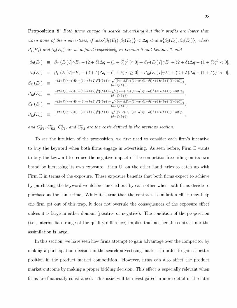
Proposition 8. Both firms engage in search advertising but their profits are lower than
when none of them advertises, if max{β1(E1), β3(E1)} < ∆q < min{β2(E1), β4(E1)}, where
β1(E1) and β2(E1) are as defined respectively in Lemma 5 and Lemma 6, and
β3(E1) ≡ β31(E1)I[γE1 + (2 + δ)∆q − (1 + δ)q0 ≥ 0] + β32(E1)I[γE1 + (2 + δ)∆q − (1 + δ)q0 < 0],
β4(E1) ≡ β41(E1)I[γE1 + (2 + δ)∆q − (1 + δ)q0 ≥ 0] + β42(E1)I[γE1 + (2 + δ)∆q − (1 + δ)q0 < 0],
β31(E1) ≡ −(2+δ)(γ+ε)E1+{3t+(δ+2)q0}(δ+1)−√
{(γ+ε)E1+(3t−q0)(1+δ)}2+18t(δ+1)(δ+3)C∗U2
(δ+1)(δ+3),
β32(E1) ≡ −(2+δ)(γ−ε)E1+{3t+(δ+2)q0}(δ+1)−√
{(γ−ε)E1+(3t−q0)(1+δ)}2+18t(δ+1)(δ+3)C∗E2
(δ+1)(δ+3),
β41(E1) ≡ −(2+δ)(γ+ε)E1−{3t−(δ+2)q0}(δ+1)+√
{(γ+ε)E1−(3t+q0)(1+δ)}2+18t(δ+1)(δ+3)C∗E2
(δ+1)(δ+3),
β42(E1) ≡ −(2+δ)(γ−ε)E1−{3t−(δ+2)q0}(δ+1)−√
{(γ−ε)E1−(3t+q0)(1+δ)}2+18t(δ+1)(δ+3)C∗U1
(δ+1)(δ+3),
and C∗E1, C∗
E2, C∗U1, and C∗
U2 are the costs defined in the previous section.
To see the intuition of the proposition, we first need to consider each firm’s incentive
to buy the keyword when both firms engage in advertising. As seen before, Firm E wants
to buy the keyword to reduce the negative impact of the competitor free-riding on its own
brand by increasing its own exposure. Firm U, on the other hand, tries to catch up with
Firm E in terms of the exposure. These exposure benefits that both firms expect to achieve
by purchasing the keyword would be canceled out by each other when both firms decide to
purchase at the same time. While it is true that the contrast-assimilation effect may help
one firm get out of this trap, it does not overrule the consequences of the exposure effect
unless it is large in either domain (positive or negative). The condition of the proposition
(i.e., intermediate range of the quality difference) implies that neither the contrast nor the
assimilation is large.
In this section, we have seen how firms attempt to gain advantage over the competitor by
making a participation decision in the search advertising market, in order to gain a better
position in the product market competition. However, firms can also affect the product
market outcome by making a proper bidding decision. This effect is especially relevant when
firms are financially constrained. This issue will be investigated in more detail in the later

29
section that proposes the extension of the model where we relax the assumption of unlimited
budgets.
4 Experimental Validation
In developing our theoretical model, we crucially relied on the assumption of the effect
of search advertising on consumer perception. In particular, we described the change in
perceived quality due to advertisement, using the following two effects: (1) the exposure
effect to capture the consumer’s tendency to positively revise their quality perception after
being exposed to the advertisement, and (2) the contrast-assimilation effect to capture the
bias of relatively evaluating two objects that are shown together. Although these are well-
documented phenomena in the literature, it is important to confirm these effects in the
context of search advertising, in justifying our model assumptions. This section summarizes
the procedure and the result of the empirical test that we conducted to validate the model
assumption.
Method We conducted an experiment where each participant was asked to rate the
quality of three products on a seven point scale, after being exposed to a search engine
result page. The study used a two (Brand owner’s advertisement: Shown or Not shown)
by three (Competitor’s advertisement: High-quality shown, Low-quality shown, or None
shown) between-subjects design. We used the keyword ‘Sony TV’. Participants who were in
the Brand owner’s advertisement Shown condition were exposed to a Sony advertisement on
the search page, and those in the Not shown condition were not shown the advertisement.
Participants who were in the Competitor’s advertisement High-quality shown condition were
exposed to a Panasonic advertisement, those in the Low-quality shown condition were ex-
posed to a Haier advertisement, and those in the None shown condition were not exposed to
any competitor’s advertisement. These stimuli are presented in Figure 5. All participants
gave ratings for Sony, Panasonic, and Haier. To ensure that Panasonic and Haier indeed are
perceived differently in quality, we tested whether their quality ratings are different using the

30
ratings given in the Brand owner advertisement Not shown by Competitor’s advertisement
None shown condition. As expected, participants gave different ratings for Panasonic and
Haier (M = 4.19, M = 2.98 respectively; t = 9.57, p < 0.001).
–Insert Figure 5–
Participants We obtained responses from 300 participants who participated in the
study through the online survey web site, www.qualtrics.com. They were randomly assigned
to one of six experimental conditions.
Results We tested the validity of our assumption directly by estimating each parameter
value using the quality rating response data. In particular, we denote the baseline quality
of each brand by qi and the exposure effect by Ei1. i can be any one of S, P , and H, which
respectively represent, Sony, Panasonic, and Haier. Note that we pooled the effect of γ into
the exposure effect ES1 and the effect of ε in EP
1 and EH1 . The contrast-assimilation effect
is given by Ei2 in the case where Sony interacts with brand i. In addition, the incremental
contrast-assimilation effect from the NY to the YY scenario is represented by δi.13 By
letting ySi denote the participants’ response of the quality rating of brand i in scenario S,
the estimating equations are given as in Table 2. Note that εSi ’s are error terms.
We obtain the parameter estimates using OLS estimation and report them in Table 3.
First, the quality ratings are positive and are in the order of Sony, Panasonic, and Haier,
which is consistent with our design. We also find the exposure effects of competitor brands
(EP1 and EH
1 ) to be positive and significant.14 Note that the exposure effects are estimated
respectively EP1 = 0.857 and EP
1 = 0.502. This result provides support for our assumption
of the exposure effect. However, the exposure effect of the brand owner (Sony) is 0.144 and
is not significantly different from zero.15 There may not be much additional gain in terms
of perceived quality by advertising to those who already recognize Sony as a high-quality
13To see the conversion of notations from Table 1 to Table 2, note that ES1 is defined to be equivalent to
(1 + γ)E1, EP1 and EH
1 are to (1− ε)E1, EP2 and EH
2 are to 12E2, and δP and δH are to 1
2δE2.14Because we test whether the exposure effect is positive, we need to use the one-tailed test, where the
p-value is given by half of that in the two-tailed test. Thus, the p-values for both parameters are given by0.00165 and 0.0400, respectively.
15In this case, p-value is 0.2370.

31
Table 2. Estimating Equations
yY YS = qS + ES
1 + EP2 + δP + εY Y
S
yY YP = qP + EP
1 − EP2 − δP + εY Y
P
yNYS = qS + EP
2 + εNYS
yNYP = qP + EP
1 − EP2 + εNY
P
yY NS = qS + ES
1 + εY NS
yY NP = qP + εY N
P
yNNS = qS + εNN
S
yNNP = qP + εNN
P
yY YS = qS + ES
1 + EH2 + δH + εY Y
S
yY YH = qH + EH
1 − EH2 − δH + εY Y
H
yNYS = qS + EH
2 + εNYS
yNYH = qH + EH
1 − EH2 + εNY
H
yY NH = qH + εY N
P
yNNH = qH + εNN
P
brand. We can interpret this as the differentiation factor γ’s being close to -1. This result
suggests that the brand owner does not always benefit from exposure of the advertisement.
Next we examine the contrast-assimilation effect. We expect a contrast in a brand that
is far apart in quality from the high-quality brand owner but an assimilation in a brand that
is close to the high-quality brand owner. Our results partially support these expectations.
Specifically, we test the hypotheses: EP2 < 0 and EH
2 > 0. When testing the hypotheses,
we reject the null hypothesis for Haier (p = 0.0408) but not for Panasonic (p = 0.9004).
Thus, the contrast effect for Haier is confirmed. Now given that EP2 is positive, we test
another hypothesis: EP2 > 0, in which case the null hypothesis is rejected at the 0.10
significance level (p = 0.0997). Thus, even for Panasonic, there is a contrast effect, rather
than an assimilation effect. It may be the case that Panasonic is not close enough to Sony
in the quality dimension. Another observation of this result is that the contrast effect is
directionally larger in Haier than in Panasonic, although the difference is not statistically

32
Table 3. Parameter Estimates
qS qP qH ES1 EP
1 EH1 EP
2 EH2 δP δH
5.525 4.102 2.755 0.144 0.857 0.502 0.299 0.409 −0.187 −0.221
(0.182) (0.142) (0.142) (0.201) (0.281) (0.287) (0.233) (0.234) (0.222) (0.228)
< .0001 < .0001 < .0001 0.4740 0.0023 0.0800 0.1997 0.0815 0.4001 0.3323
Standard error are in parenthesis. The last row represents the p-value in a two-tailed test.
significant. This provides partial support for our conjecture.
Finally, we observe that none of the δ’s are significant. This implies that there does
not exist an incremental contrast effect in the YY scenario. However, we cannot conclude
whether this is only for this keyword or also true in general. We may need to collect more
data using a different set of keywords to answer this question.
In sum, we have shown that the assumptions are generally consistent with what we
observe from the experimental data. Especially, both the exposure effect of the competitors
and the contrast effect were confirmed by data. In fact, the estimating equations are fitted
very well with the adjusted-R2 being 0.92, which may provide stronger support for the general
quality specification in our model. Thus we complete this section by concluding that our
model is well-grounded.
5 Proposed Work
In the main analysis, we have assumed that advertisers have unlimited budgets. However, in
reality, firms allocate a limited amount of budget to advertising. Thus, it is important to con-
sider advertisers with insufficient resources and investigate how their behavior changes due
to financial constraints. In this section, we propose an extension of the model incorporating
this aspect and briefly discuss our preliminary analysis and the expected results.
As before, we have two stages: advertising and pricing. However, because the pricing
decisions given for the perceived quality ∆q remain the same, we only consider the advertising

33
decisions. We start by assuming that the advertising budgets of both firms are binding at
the first slot under the YY scenario. This implies that scenarios YY1 (where both firms
advertise and Firm E takes the first slot) and YY2 (where both firms advertise and Firm
U takes the first slot) cannot last to the end of the designated period. In particular, in
scenario YY1, Firm E can take the first slot for only KE
CE1fraction of the time. Then, Firm
E exhausts its budget and only Firm U is left to continue advertising until the end of the
period. Note that Firm U has sufficient budget to cover the cost of advertising in the NY
scenario. Similarly, YY2 scenario becomes YN after KE
CE1fraction of the period, because Firm
U drops out due to budget constraint. Accordingly, we revise the perceived quality of each
product in the above two scenarios as follows:
˜qY Y 1i ≡
( KE
CE1
)qY Y 1i +
(1− KE
CE1
)qNYi (12)
˜qY Y 2i ≡
( KU
CU1
)qY Y 2i +
(1− KU
CU1
)qY Ni (13)
where ˜qSi and qS
i respectively denote the perceived quality in scenario S with and without
budget constraint. Note that the expression for qSi is given in Table 1. The other scenarios
are not affected by the budget constraint and thus ˜qSi = qS
i , (S = Y N, NY ).
As before, Firm E may choose the first slot or the second slot in equilibrium. We first
characterize the bidding equilibrium in each case. Our preliminary analysis suggests the
following behavior of both firms in the bidding game.
Result 1. In the bidding game, under some conditions, the second slot winner may have an
incentive to increase its own bid as high as possible in order to increase the cost of the first
slot winner.
In the previous section, we saw each firm strategically make a participation decision in the
keyword auction looking forward the outcome of the product market competition. Likewise,
firms can influence the competitive horizon of the product market by strategically setting
their bid amount. In particular, the above result shows that firms may have an incentive to
increase the cost of their budget-constrained rival by raising their own bid amount. Note

34
that this is possible because the search engine uses the generalized second price auction
rule, where the payment of the winner depends on the next winner’s bid amount. Thus, the
second slot winner can effectively damage its competitor in the first slot, but not vice versa.
In some cases, a firm may use this strategy as a retaliation when it loses the first slot to its
competitor. However, the firm also benefits itself by using this strategy.
Raising rival’s cost can be especially profitable, when the high cost of advertising quickly
runs up the competitor’s advertising budget. By doing so, the firm is able to constrain the
period during which the competitor’s advertisement is shown and thus, restrict the competi-
tor’s ability to charge higher prices. There has been empirical evidence of the existence of
this behavior (Ganchev et al. 2007).
However, it may not be profitable when they can get additional benefit from being com-
pared with the competitor. In particular, our preliminary analysis suggests that if the
contrast effect (for Firm E) or the assimilation effect (for Firm U) is large enough, they may
prefer to stay in the YY scenario rather than exhausting the competitor’s budget and thus
being left alone. Thus, even though the strategy is generally effective in occupying a better
position in the product market competition, we may not observe this behavior all the time.
Recall that with unlimited budgets, the solution is specified up to an interval. One
implication of the above result is that by considering budget-constrained advertisers, we
can actually pin down their bidding strategies in equilibrium. In particular, the second slot
winner makes its bid at either the maximum or the minimum amount. To see the intuition,
consider that because of the budget constraint, the second slot winner is now able to affect
the duration of its competitor’s advertisement and thus the timing of the transition from one
scenario to another. Then depending on the relative profitability of the scenarios before and
after the change, the second slot winner may maximize or minimize the duration. Thus we
observe the second slot winner choosing either the maximum or the minimum bid amount
in its range.
Given this analysis of the bidding equilibrium in the YY scenario with budget constraint,

35
we can investigate the impact of the budget constraint on the equilibrium participation
decision. Based on the participation equilibrium, we expect to obtain the following set
of results. First, when both firms’ budgets are constrained, obtaining the YY scenario is
less likely in equilibrium. This is because now the keyword purchase option becomes less
attractive to each firm. Second, for the same level of the exposure effect and the contrast-
assimilation effect, at which Firm E advertises only for a defensive purpose (Proposition 3),
it may refuse to advertise at all. This may be because either Firm E cannot gain much by
defending even in the presence of the competitor’s threat, or the competitor’s threat is now
gone, or both. Finally, if Firm U is budget-constrained, Firm E can protect its own brand
name even given small contrast effects. This is because Firm E’s purchase becomes a bigger
threat to the competitor and thus preclusion becomes easier.
6 Conclusion
In this paper, we aim to understand when and why we observe different patterns of branded
keyword purchase behavior. To investigate these issues, we developed a duopoly model
where two firms offer horizontally and vertically differentiated products and engage in brand
advertising in the search engine. We analyzed our theoretical model without budget con-
straint, tested the assumptions using an experiment, and proposed the model with budget
constraint.
Our analysis helps us understand the questions we raised in the introduction.
1. When do we observe one pattern over the other? When the exposure effect is not
large, neither firm buys the branded keyword because their cost of advertising is not justified.
If the exposure effect is above a certain threshold, both firms become interested in buying
the keyword and thus, the contrast-assimilation effect comes into play. If the contrast effect
is strong, only the brand owner is observed in equilibrium, but if the assimilation effect is
strong, only the competitor appears in the sponsored links. If neither effect (contrast or
assimilation) is large, we observe both firms advertising together. Because the impact of the

36
contrast-assimilation effect is asymmetric, the firm that is unfavorably affected by a strong
contrast or assimilation effect gives up advertising, but both firms freely choose to advertise
if neither effect is strong.
2. Why do brand owners buy their own branded keyword? Why do some firms forgo
the opportunity to advertise under a well-known brand’s name? When the exposure effect
is weak and neither contrast nor assimilation effect is large, the brand owner buys its own
keyword, but only for a defensive purpose. It may not want to advertise but does so only
because its competitor advertises. The competitor’s purchase may hurt the brand owner and
thus it needs to defend itself by matching the competitor’s purchase decision. However, if
both the exposure effect and the contrast effect are strong enough, the brand owner may buy
the keyword in order to preclude its competitor. In fact, the preclusion is possible because
the contrast effect is large enough. In this case, the competitor cannot buy because it is
precluded, and not because it does not want to buy.
Moving towards the case where firms have limited advertising budgets, we identified an
interesting pattern in the bidding equilibrium: when in the second slot, both firms may have
an incentive to increase their own bid as high as possible in order to quickly exhaust the
other firm’s budget. By doing so, each firm can confine the profitability of the other firm.
Given this derivation of bidding equilibrium, it is possible to derive the keyword purchase
decision of both firms and thus investigate the impact of budget on purchase decisions. From
this analysis, we expect to derive the following results: First, budget constraints make it less
likely that both firms advertise together; Second, the need for a defensive purchase by the
brand owner may be reduced as the budget becomes more binding; Third, the preclusion is
more prevalent with more binding budgets.
Finally, our experimental investigation shows that the exposure effect of the competitors
exists, while that of the brand owner may be weak or insignificant. It also confirms the
existence of a statistically significant contrast effect. However, we did not see any case of an
assimilation effect. This may be because the brands used as the competitor in our experiment

37
are not close enough to the brand owner in terms of quality.
Our work contributes to the search advertising literature in that this is the first attempt
to model the impact of search advertising on brand value. Also, by connecting the two
competitive horizons of both markets, we offer insight on how firms behave optimally. The
conditions derived for each equilibrium and for each particular case (i.e., the defensive pur-
chase and the preclusion) provide a normative guideline on when to buy one’s own keyword
and when to buy a competitor’s keyword. Finally, our analysis has a policy implication. By
considering the contrast effect, we can identify the case where the brand owner is actually
better off by a competitor’s trademark infringement. This may help resolve some lawsuits
against Google.
Beyond what we have found in this paper, there are many directions for further analysis
and future research. First, we will conduct a complete analysis of the budget constrained
case. Second, one can investigate the changes in the purchase decision due to changes in
the brand awareness, in addition to the quality perception. Third, other advertisers such
as retailers that were ignored in our model can be explicitly modeled. Finally, it will be
an interesting future research to investigate how the consumer inference on the competitor’s
product quality is affected by the brand owner’s product quality in various circumstances.

38
References
Anderson, R.E. (1973), “Consumer Dissatisfaction: The Effect of Disconfirmed Expectancyon Perceived Product Performance,” Journal of Marketing Research, 10(1), 38-44.
Athey, S., and G. Ellison (2008), “Position Auctions with Consumer Search,” Working paper,Harvard University.
Balachander, S. and K. Kannan (2008), “A Theoretical and Empirical Analysis of AlternateAuction Policies for Search Advertisements,” Working paper, Purdue University.
Batra, R., J.G. Myers, and D.A. Aaker (1996), Advertising Management, Prentice Hall,Upper Saddle River, NJ.
Chen, Y. and C. He (2006), “Paid Placement: Advertising and Search on the Internet,”Working paper, University of Colorado and Boulder.
Dellarocas, C. and S. Viswanathan (2008), “The Holy Grail of Advertising? AllocativeEfficiency and Revenue Implications of “Pay-Per-Action” Advertising in Environmentswith Quality Uncertainty,” Working paper, University of Maryland.
Desai, P., and W. Shin (2006), “Allocation Mechanisms in Search Advertising: A Two-SidedMarket Approach,” Working paper, Duke University.
Desai, P., and W. Shin (2009), “Advertiser-Specific Minimum Bids and Advertising Budgetsin Keyword Search Auctions,” Working paper, Duke University.
Diamond, P.A. (1971), “A Model of Price Adjustment,” Journal of Economic Theory, 3,156-168.
Edelman, B., M. Ostrovsky, and M. Schwarz (2007), “Internet Advertising and the Gener-alized Second-Price Auction: Selling Billions of Dollars Worth of Keywords,” AmericanEconomic Review, 97(1), 242-258.
Enquiro Research and Google (2007), The Brand Lift of Search: Enquiro Online Survey andEye Tracking Study, July 2007.
Ganchev, K., A. Kulesza, J. Tan, G. Ryan, Q. Liu, and M. Kearns (2007), “EmpiricalPrice Modeling for Sponsored Search,” Proceedings of the 3rd International WorkshopOn Internet And Network Economics, San Diego, CA, Springer.
Ghose, A. and S. Yang (2009) “An Empirical Analysis of Search Engine Advertising: Spon-sored Search in Electronic Markets,” Management Science, Forthcoming.
Google and Media Screen (2008), The Brand Value of Search: Consumer Packaged GoodsIndustry Study, July 2008.
Grewal, D., R. Krishnan, J. Baker, and N. Borin (1998), “The Effects of Store Name, BrandName, and Price Discounts on Consumers’ Evaluations and Purchase Intentions,” Journalof Retailing, 74(3), 331-352.
Helft, M. (2009) “Companies Object to Google Policy on Trademarks,” The New York Times,May 14, 2009.

39
Hovland, C.I., O.J.Harvey, and M. Sherif (1957), “Assimilation and Contrast Effects inReactions to Communication and Attitude Change,” Journal of Abnormal and SocialPsychology, 55, 244-252.
Jerath, K., L. Ma, Y-H. Park, and K. Srinivasan (2009), “A “Position Paradox” in SponsoredSearch Auctions,” Working paper, Carnegie Mellon University.
Katona, Z., and M. Sarvary (2008), “The Race for Sponsored Links: Bidding Patterns forSearch Advertising,” Working paper, Haas School of Business, University of California,Berkeley.
Lahaie (2006), “An Analysis of Alternative Slot Auction Designs for Sponsored Search,” InProceeding. Second Workshop on Sponsored Search Auctions at ACM Conference onElectronic Commerce (EC’06), June 11, Ann Arbor, MI.
Ledgerwood, A., and S. Chaiken (2007), “Priming Us and Them: Automatic Assimilationand Contrast in Group Attitudes,” Journal of Personality and Social Psychology, 93(6),940-956.
Lichtenstein D.R., and W.O. Bearden (1989), “Contextual Influences on Perceptions ofMerchant-Supplied Reference Prices,” Journal of Consumer Research, 16, 55-66.
Liu, D., J. Chen, and A. B. Whinston (2008) “Ex-Ante Information and the Design ofKeyword Auctions,” Information Systems Research, Forthcoming.
Mussweiler, T. (2001), “Focus of Comparisons as a Determinant of Assimilation VersusContrast in Social Comparison,” Personality and Social Psychology Bulletin, 27(1), 38-47.
Mussweiler, T. (2003), “Comparison Processes in Social Judgment: Mechanisms and Conse-quences,” Psychological Review, 110(3), 472-489.
Orey, M. (2009) “Google’s Rival Keyword Sales Go Wide,” Businessweek, May 11, 2009.
Olshavsky, R.W., and J.A. Miller (1972), “Consumer Expectations, Product Performance,and Perceived Quality,” Journal of Marketing Research, 9(1), 19-21.
Online Publishers Association (2009), The Silent Click: Building Brands Online, June 2009.
Rutz, O. and R. Bucklin (2007a) “From Generic to Branded: A Model of Spillover Dynamicsin Paid Search Advertising,” Working paper, Yale University.
Rutz, O. and R. Bucklin (2007b) “A Model of Individual Keyword Performance in PaidSearch Advertising,” Working paper, Yale University.
Salop, S.C., and D.T., Scheffman (1983) “Raising Rivals’ Costs,” AEA Papers and Preceed-ings, 73(2), 267-271.
Salop, S.C., and D.T., Scheffman (1987) “Cost-Raising Strategies,” Journal of IndustrialEconomics, 36(1), 19-34.
Sherif, M, D. Taub, and C.I. Hovland (1958), “Assimilation and Contrast Effects of Anchor-ing Stimuli on Judgments,” Journal of Experimental Psychology, 55(2), 150-155.

40
Stewart, K.J., and R.A. Malaga (2009), “Contrast and Assimilation Effects on Consumers’Trust in Internet Companies,” International Journal of Electronic Commerce, 13(3), 71-93.
Wilbur, K., and Y. Zhu (2008) “Click Fraud,” Marketing Science, 28(2), 293-308.
Varian, H. (2007) “Position Auctions,” International Journal of Industrial Organization, 25,1163-1178.
Xu, L., J. Chen, and A.B. Whinston (2009) “To Place Better or Price Cheaper? Biddingand Pricing under Keyword Advertising,” Working paper, University of Texas, Austin.
Yao, S. and C. Mela (2009) “A Dynamic Model of Sponsored Search Advertising,” Workingpaper, Duke University.
Zajonc, R.B. (1968) “Attitudinal Effects of Mere Exposure,” Journal of Personality andSocial Psychology, 9, 1-27.

41
Figure 1: Examples of Branded Keywords

42
Figure 2: Parameter Space (Shaded Area)(∆q = 100, t = 50, δ = 0.9, γ = −0.75, ε = 0.1)
Figure 3: An Illustration of Participation Equilibrium

43
Figure 4: Regions of Strategic Purchase Decision

44
Figure 5: Stimuli used in the Experiment
Shown by High-quality shown condition Not shown by High-quality shown condition
Shown by Low-quality shown condition Not shown by Low-quality shown condition
Shown by None shown condition Not shown by None shown condition

45
Appendix
Definition of b0X in footnote 2
We define b0X as follows.
b0X ≡ min{b0
X1, b0X2, b
0X3}
where
b0X1 ≡ I∗ (1+γ){3t(3+δ)−q0(1+δ)}{3t(5+γ+3δ(1+γ)+4ε)+k(1+γ)(1+δ)}
18ts1rX(2+γ+δ+γδ+ε)2+ (1− I∗) (9t−q0)(1+γ){3t(9+3γ)+q0(1+γ)}
18ts1rX(3+2γ)2
with I∗ = I[{2(1 + γ − ε) + δ}{3t((3− δ)γ + 3(1− ε))− q0(1 + γ(1 + δ) + 2δ − ε)} ≤ 0],
b0X2 ≡ I∗ {3t(7+2δ+5γ+δγ−ε)−q0(1+γ+(2+γ)δ−ε)}2−(1+γ)2{3t(3+δ)−q0(1+δ)}2
18ts1rX(2+γ+δ+γδ+ε)2
+(1− I∗)9t2(7γ2+30γ+27)+(1+γ)2q0(18t−q0)}18ts1rX(3+2γ)2
,
b0X3 ≡
(3t− q0)δ{3t(8 + 3δ) + δq0}18ts2rX(2 + δ)2
and,
b0X4 ≡
q0(1 + δ){6t + q0(1 + δ)}18ts2rX
In fact, bX ≤ b0X1 ensures that Firm E buys the keyword in the presence of Firm
X, while bX ≤ b0X2 ensures that Firm U buys the keyword in the presence of Firm X.
Similarly, bX ≤ b0X3 ensures Firm E’s purchase of the keyword in the presence of Firm U
and Firm X, while bX ≤ b0X4 guarantees Firm U’s purchase of the keyword in the presence
of Firm E and Firm X. 2
Proof of Lemma 1
The profit functions given in equations (5) and (6) are concave in their own prices. Thus,
by taking the first derivatives and setting them to be zero, we obtain two equations of
prices. Then, simultaneously solving them, we obtain equilibrium prices. Finally, plug-
ging them back into equations (3), (4), (5), and (6), we derive the equilibrium demands
and profits. 2

46
Proof of Proposition 1
First, note that by Lemma 1, the equilibrium prices and sales are given by p∗E = t + ∆q3
,
p∗U = t − ∆q3
, D∗E = 3t+∆q
6t, and D∗
U = 3t−∆q6t
. From the expressions given Table 1, ∆q in
each scenario is given as follows:
∆qNN = ∆q
∆qY N = ∆q + (1 + γ)E1
∆qNY = ∆q − E1 + E2
∆qY Y 1 = ∆q + (γ + ε)E1 + (1 + δ)E2
∆qY Y 2 = ∆q + (γ − ε)E1 + (1 + δ)E2.
Then, the first part of the proposition is proved by considering the following two
scenarios:
• In Scenario YN: Firm E is the advertising firm and,∂p∗E∂E1
= 1+γ3
> 0 and∂D∗
E
∂E1= 1+γ
6t> 0,
while Firm U is the non-advertising firm, and∂p∗U∂E1
= −1+γ3
< 0 and∂D∗
U
∂E1= −1+γ
6t< 0.
• In Scenario NY: Firm U is the advertising firm and,∂p∗U∂E1
= 13
> 0 and∂E∗
U
∂E1= 1
6t> 0,
while Firm E is the non-advertising firm and,∂p∗E∂E1
= −13
< 0 and∂D∗
E
∂E1= − 1
6t< 0.
The second part is proved by considering the following two scenarios:
• In Scenario YY1:∂p∗E∂E1
= γ+ε3
> 0,∂D∗
E
∂E1= γ+ε
6t> 0,
∂p∗U∂E1
= −γ+ε3
< 0, and∂D∗
U
∂E1= −γ+ε
6t<
0, if and only if γ + ε > 0, where γ + ε denotes the relative size of the exposure effect
of Firm E, compared with that of Firm U.
• In Scenario YY2:∂p∗E∂E1
= γ−ε3
> 0,∂D∗
E
∂E1= γ−ε
6t> 0,
∂p∗U∂E1
= −γ−ε3
< 0, and∂D∗
U
∂E1= −γ−ε
6t<
0, if and only if γ − ε > 0, where γ − ε denotes the relative size of the exposure effect
of Firm E, compared with that of Firm U. 2
Proof of Proposition 2
First note by definition, that there is a contrast if E2 > 0 and an assimilation if E2 < 0.
Thus,∂(·)∗i∂E2
> 0 means that the equilibrium quantity (price or sales) of Firm i increases
with a contrast but decreases with an assimilation. As in the previous proof, we consider
the derivatives in the following scenarios.

47
• In Scenario NY:∂p∗E∂E2
= 13
> 0,∂D∗
E
∂E2= 1
6t> 0,
∂p∗U∂E2
= −13
< 0, and∂D∗
U
∂E2= − 1
6t< 0.
Thus, with a contrast, Firm E’s price and sales go up, while they go down with an
assimilation. The reverse is true for Firm U.
• In Scenarios YY1 and YY2:∂p∗E∂E2
= 1+δ3
> 0,∂D∗
E
∂E2= 1+δ
6t> 0,
∂p∗U∂E2
= −1+δ3
< 0, and∂D∗
U
∂E2= −1+δ
6t< 0. The same conclusion as in Scenario NY can be reached in this case.
• In Scenarios NN and YN:∂p∗E∂E2
= 0. This proves the first line of the proposition. 2
Proof of Lemma 2
Let πij denote the profit Firm i earns from the product market when taking the jth slot
in the search advertising market. Suppose Firm i takes the first slot and Firm i′ takes
the second slot in equilibrium. Then by definition of Symmetric Nash Equilibrium, we
have:
πi1 − s1ri′bi′ ≥ πi2 − s2rXbX (A1)
πi′2 − s2rXbX ≥ πi′1 − s1ri′bi′ . (A2)
Summing two inequalities, we obtain the following condition:
πi1 + πi′2 ≥ πi2 + πi′1. (A3)
Rearranging the order, we have:
πi1 − πi2 ≥ πi′1 − πi′2, (A4)
which implies that in equilibrium, the firm with higher incremental profit of moving from
the second slot to the first slot wins the first slot. Thus, Firm E takes the first slot, if
and only if
πE1 − πE2 ≥ πU1 − πU2. (A5)
From the product market competition equilibrium, we know,
πE1 = {3t+(γ+ε)E1+(2+δ)∆q−(1+δ)q0}2
18t(A6)
πU2 = {3t−(γ+ε)E1−(2+δ)∆q+(1+δ)q0}2
18t(A7)
πE2 = {3t+(γ−ε)E1+(2+δ)∆q−(1+δ)q0}2
18t(A8)
πU1 = {3t−(γ−ε)E1−(2+δ)∆q+(1+δ)q0}2
18t. (A9)

48
Note that we replace E2 by ∆q − q0 in deriving the above profits. Therefore, equation
(A5) is equivalent to,
8εE1{γE1 + (2 + δ)∆q − (1 + δ)q0} ≥ 0. (A10)
Then the result follows. 2
Proof of Lemma 3
By inequalities in (A1) and (A2), the second slot winner’s equilibrium bid bi′ must satisfy
πi′1 − πi′2 + s2rXbX ≤ s1ri′bi′ ≤ πi1 − πi2 + s2rXbX . (A11)
Noting that Ci1 ≡ s1ri′bi′ , the rest follows from the expressions given in (A6)-(A9). 2
Proof of Lemma 4
Let Π(··)i denote Firm i’s profit under scenario (··). Then when Firm U does not buy,
Firm E buys if and only if ΠY NE ≥ ΠNN
E , where
ΠY NE = {3t+(1+γ)E1+∆q}2
18t− C∗
E0 (A12)
ΠNNE = {3t+∆q}2
18t. (A13)
This is equivalent to
E1 ≤−(3t+∆q)−
√(3t+∆q)2+18tC∗
E0
1+γor E1 ≥
−(3t+∆q)+√
(3t+∆q)2+18tC∗E0
1+γ. (A14)
Recall from equation (7), that the parameter space is confined such that E1 ≥ −3t+∆q1+γ
.
Thus, we rewrite the condition in (A14) as,
E1 ≥ α1(E2) ≡−(3t+∆q)+
√(3t+∆q)2+18tC∗
E0
1+γ. (A15)
Also, note that bX ≤ b0X1 implies that there exists at least one point in the parameter
space that satisfies (A15).
Now when Firm E does not buy, Firm U buys if and only if ΠNYU ≥ ΠNN
U , where
ΠNYU = {3t+E1−2∆q+q0}2
18t− C∗
U0 (A16)
ΠNNU = {3t−∆q}2
18t. (A17)
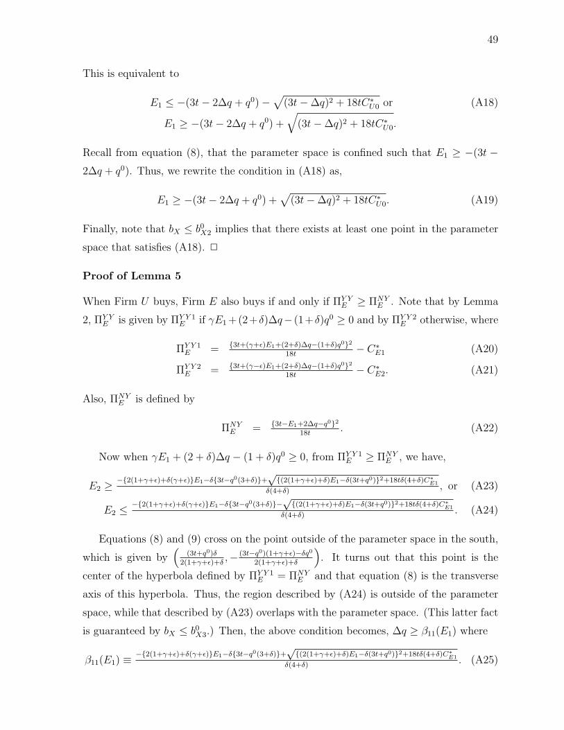
49
This is equivalent to
E1 ≤ −(3t− 2∆q + q0)−√
(3t−∆q)2 + 18tC∗U0 or (A18)
E1 ≥ −(3t− 2∆q + q0) +√
(3t−∆q)2 + 18tC∗U0.
Recall from equation (8), that the parameter space is confined such that E1 ≥ −(3t −2∆q + q0). Thus, we rewrite the condition in (A18) as,
E1 ≥ −(3t− 2∆q + q0) +√
(3t−∆q)2 + 18tC∗U0. (A19)
Finally, note that bX ≤ b0X2 implies that there exists at least one point in the parameter
space that satisfies (A18). 2
Proof of Lemma 5
When Firm U buys, Firm E also buys if and only if ΠY YE ≥ ΠNY
E . Note that by Lemma
2, ΠY YE is given by ΠY Y 1
E if γE1 +(2+δ)∆q− (1+δ)q0 ≥ 0 and by ΠY Y 2E otherwise, where
ΠY Y 1E = {3t+(γ+ε)E1+(2+δ)∆q−(1+δ)q0}2
18t− C∗
E1 (A20)
ΠY Y 2E = {3t+(γ−ε)E1+(2+δ)∆q−(1+δ)q0}2
18t− C∗
E2. (A21)
Also, ΠNYE is defined by
ΠNYE = {3t−E1+2∆q−q0}2
18t. (A22)
Now when γE1 + (2 + δ)∆q − (1 + δ)q0 ≥ 0, from ΠY Y 1E ≥ ΠNY
E , we have,
E2 ≥−{2(1+γ+ε)+δ(γ+ε)}E1−δ{3t−q0(3+δ)}+
√{(2(1+γ+ε)+δ)E1−δ(3t+q0)}2+18tδ(4+δ)C∗
E1
δ(4+δ), or (A23)
E2 ≤−{2(1+γ+ε)+δ(γ+ε)}E1−δ{3t−q0(3+δ)}−
√{(2(1+γ+ε)+δ)E1−δ(3t+q0)}2+18tδ(4+δ)C∗
E1
δ(4+δ). (A24)
Equations (8) and (9) cross on the point outside of the parameter space in the south,
which is given by(
(3t+q0)δ2(1+γ+ε)+δ
,− (3t−q0)(1+γ+ε)−δq0
2(1+γ+ε)+δ
). It turns out that this point is the
center of the hyperbola defined by ΠY Y 1E = ΠNY
E and that equation (8) is the transverse
axis of this hyperbola. Thus, the region described by (A24) is outside of the parameter
space, while that described by (A23) overlaps with the parameter space. (This latter fact
is guaranteed by bX ≤ b0X3.) Then, the above condition becomes, ∆q ≥ β11(E1) where
β11(E1) ≡−{2(1+γ+ε)+δ(γ+ε)}E1−δ{3t−q0(3+δ)}+
√{(2(1+γ+ε)+δ)E1−δ(3t+q0)}2+18tδ(4+δ)C∗
E1
δ(4+δ). (A25)

50
Finally, when γE1 + (2 + δ)∆q − (1 + δ)q0 < 0, from ΠY Y 2E ≥ ΠNY
E , we have,
E2 ≥−{2(1+γ−ε)+δ(γ−ε)}E1−δ{3t−q0(3+δ)}+
√{(2(1+γ−ε)+δ)E1−δ(3t+q0)}2+18tδ(4+δ)C∗
E1
δ(4+δ), or (A26)
E2 ≤−{2(1+γ−ε)+δ(γ−ε)}E1−δ{3t−q0(3+δ)}−
√{(2(1+γ−ε)+δ)E1−δ(3t+q0)}2+18tδ(4+δ)C∗
E1
δ(4+δ). (A27)
Similarly, equations (8) and (10) defines a point outside of the parameter space in the
south, which is given by(
(3t+q0)δ2(1+γ−ε)+δ
,− (3t−q0)(1+γ−ε)−δq0
2(1+γ−ε)+δ
)and turns out to be the center
of the hyperbola defined by ΠY Y 2E = ΠNY
E . Again, equation (8) is the transverse axis of
this hyperbola. Thus, the region described by (A27) is outside of the parameter space,
while that described by (A26) overlaps with the parameter space, by bX ≤ b0X3. Thus,
the above condition becomes, ∆q ≥ β12(E1) where
β12(E1) ≡−{2(1+γ−ε)+δ(γ−ε)}E1−δ{3t−q0(3+δ)}+
√{(2(1+γ−ε)+δ)E1−δ(3t+q0)}2+18tδ(4+δ)C∗
E1
δ(4+δ). (A28)
Thus follows the lemma. 2
Proof of Lemma 6
When Firm E buys, Firm U also buys if and only if ΠY YU ≥ ΠY N
U . Note that by proposition
1, ΠY YU is given by ΠY Y 1
U if γE1 +(2+δ)∆q− (1+δ)q0 ≥ 0 and by ΠY Y 2U otherwise, where
ΠY Y 1U = {3t−(γ+ε)E1−(2+δ)∆q+(1+δ)q0}2
18t− C∗
U2 (A29)
ΠY Y 2U = {3t−(γ−ε)E1−(2+δ)∆q+(1+δ)q0}2
18t− C∗
U1. (A30)
Also, ΠY NU is defined by
ΠY NU = {3t−(1+γ)E1−∆q}2
18t. (A31)
Now when γE1 + (2 + δ)∆q − (1 + δ)q0 ≥ 0, from ΠY Y 1U ≥ ΠY N
U , we have,
E2 ≥2{(1−γ−2ε)−δ(γ+ε)}E1+6t(1+δ)+2q0(2+δ)(1+δ)+
√{(2+γ−ε+δ(γ+1))E1−(3t−q0)(1+δ)}2+72t(3+δ)(1+δ)C∗
U2
2(3+δ)(1+δ), or(A32)
E2 ≤2{(1−γ−2ε)−δ(γ+ε)}E1+6t(1+δ)+2q0(2+δ)(1+δ)−
√{(2+γ−ε+δ(γ+1))E1−(3t−q0)(1+δ)}2+72t(3+δ)(1+δ)C∗
U2
2(3+δ)(1+δ).(A33)
By equations (7) and (9), one vertex in the north of the parameter space is given by((1+δ)(3t−q0)
2+γ−ε+δ(1+γ), 3t(1−ε)−q0(1+γ)(1+δ)
2+γ−ε+δ(1+γ)
). It also turns out that this point is the center of the
hyperbola defined by ΠY Y 1U = ΠY N
U and that equation (7) is the transverse axis of this
hyperbola. Thus, the region described by (A32) is outside of the parameter space, while

51
that described by (A33) overlaps with the parameter space. (This latter fact is guaranteed
by bX ≤ b0X4.) Therefore, the condition for ΠY Y 1
U ≥ ΠY NU becomes ∆q ≤ β21, where
β21(E1) ≡2{1−γ−2ε)−δ(γ+ε)}E1+6t(1+δ)+2q0(2+δ)(1+δ)−
√{(2+γ−ε+δ(γ+1))E1−(3t−q0)(1+δ)}2+72t(3+δ)(1+δ)C∗
U2
2(3+δ)(1+δ).(A34)
When γE1 + (1 + δ)∆q − (1 + δ)q0 < 0, from ΠY Y 2U ≥ ΠY N
U , we have,
E2 ≥2{1−γ+2ε)−δ(γ−ε)}E1++6t(1+δ)+2q0(2+δ)(1+δ)+
√{(2+γ+ε+δ(γ+1))E1−(3t−q0)(1+δ)}2+72t(3+δ)(1+δ)C∗
U2
2(3+δ)(1+δ), or(A35)
E2 ≤2{1−γ+2ε)−δ(γ−ε)}E1++6t(1+δ)+2q0(2+δ)(1+δ)−
√{(2+γ+ε+δ(γ+1))E1−(3t−q0)(1+δ)}2+72t(3+δ)(1+δ)C∗
U2
2(3+δ)(1+δ).(A36)
As above, ΠY Y 2U = ΠY N
U defines a hyperbola with the center(
(1+δ)(3t−q0)2+γ+ε+δ(1+γ)
, 3t(1+ε)−q0(1+γ)(1+δ)2+γ+ε+δ(1+γ)
)(which is outside, in the north of the parameter space) and equation (7) is again the
transverse axis of this hyperbola. Thus, the region described by (A35) is outside of the
parameter space, while that described by (A36) overlaps with the parameter space, by
bX ≤ b0X4. Therefore, the condition for ΠY Y 2
U ≥ ΠY NU becomes ∆q ≤ β22(E1), where
β22(E1) ≡2{1−γ+2ε)−δ(γ−ε)}E1++6t(1+δ)+2q0(2+δ)(1+δ)−
√{(2+γ+ε+δ(γ+1))E1−(3t−q0)(1+δ)}2+72t(3+δ)(1+δ)C∗
U2
2(3+δ)(1+δ).(A37)
This completes the proof. 2
Proof of Proposition 3
Suppose E1 < min{α1(∆q), α2(∆q)}. Then, by the first part of Lemma 4, Firm E has
no incentive to deviate from the NN scenario. Likewise, by the second part of Lemma 4,
Firm U does not have an incentive to deviate from the NN scenario. Thus, NN scenario
emerges as an equilibrium if E1 < min{α1(∆q), α2(∆q)}. 2
Proof of Proposition 4
We prove the proposition in three parts. First, we derive the condition for YN to be
observed in equilibrium. By Lemma 4, if E1 > α1(∆q), Firm E has no incentive to
deviate from the YN scenario. In addition, if ∆q ≥ β2(E1), by Lemma 6, Firm U does
not have an incentive to deviate from the YN scenario either. Thus, YN is observed when
both E1 > α1(∆q) and ∆q ≥ β2(E1) are satisfied.
Next, we prove the NY equilibrium. By Lemma 4, if E1 > α2(∆q), Firm U has no
incentive to deviate from NY scenario. Likewise, if ∆q ≤ β1(E1), by Lemma 5, Firm E
has no incentive to deviate from NY. Thus, we obtain the NY equilibrium when both
E1 > α2(∆q) and ∆q ≤ β1(E1) hold.

52
Finally, combining the results from Lemma 5 and Lemma 6, we obtain the YY equi-
librium if β2(E1) < ∆q < β1(E1).2
Proof of Proposition 5
First, by proposition 2, YY scenario emerges as an equilibrium as long as β2(E1) < ∆q <
β1(E1), even with additional condition on E1. Now, the defensive strategy is defined in
the text, as follows: (1) Firm E does not buy the keyword if Firm U also does not buy the
keyword, but (2) Firm E buys the keyword if Firm U buys the keyword. There conditions
are equivalent to (1): ΠNNE ≥ ΠY N
E and (2): ΠY YE ≥ ΠNY
E . Finally, to ensure that Firm U
buys the keyword in equilibrium so that Firm E’s defensive strategy is triggered, we need
an additional condition (3): ΠY YU ≥ ΠY N
U . By Lemma 5 and Lemma 6, the conditions
(1) and (3) are translated into β2(E1) < ∆q < β1(E1), and by Lemma 4, the second
condition is equivalent to E1 ≤ α1(∆q). 2
Proof of Proposition 6
The effective deterrence of purchase of Firm U by Firm E is defined as follows in the
text: (1) Firm U wants to buy the keyword without Firm E’s buying but (2) it does not
want to buy if Firm E buys. (3) Knowing this, Firm E buys the keyword if Firm U buys.
These conditions are translated as follows:
(1) ΠNYU ≥ ΠNN
U , which is equivalent to E1 > α2(∆q) by Lemma 4,
(2) ΠY NU ≥ ΠY Y
U , which is equivalent to ∆q > β2(E1) by Lemma 6, and
(3) ΠY YE ≥ ΠNY
E , which is equivalent to ∆q > β1(E1) by Lemma 5.
Therefore, we have E1 > α2(∆q) and ∆q > max{β1(E1), β2(E1)}. 2
Proof of Proposition 7
The proof here is similar to that of Proposition 6. The conditions are the same as in
Proposition 6, with Firm E and Firm U switched. Then the conditions are translated as
follows:
(1) ΠY NE ≥ ΠNN
E , which is equivalent to E1 > α1(∆q) (by Lemma 4),
(2) ΠNYE ≥ ΠY Y
E , which is equivalent to ∆q < β1(E1) (by Lemma 5), and
(3) ΠY YU ≥ ΠY N
U , which is equivalent to ∆q < β2(E1) (by Lemma 6).
Therefore, we have E1 > α1(∆q) and ∆q < min{β1(E1), β2(E1)}. 2

53
Proof of Proposition 8
The prisoner’s dilemma case is obtained when both firms make less profits in YY scenarios
than in NN scenario but both buy the keyword in equilibrium. Thus, the conditions are
given as follows:
(1) β1(E1) < ∆q < β2(E1), which ensures that in equilibrium both firms buy the keyword,
by Proposition 5 and Proposition 6,
(2-1) If γE1 + (2 + δ)∆q − (1 + δ)q0 ≥ 0: ΠY Y 1E ≤ ΠNN
E and ΠY Y 1U ≤ ΠNN
U , which are
respectively equivalent to β31(E1) ≤ ∆q ≤ β33(E1) and β43(E1) ≤ ∆q ≤ β41(E1), where
β31(E1) ≡−(2+δ)(γ+ε)E1+{3t+(δ+2)q0}(δ+1)−
√{(γ+ε)E1+(3t−q0)(1+δ)}2+18t(δ+1)(δ+3)C∗
U2
(δ+1)(δ+3),
β33(E1) ≡−(2+δ)(γ+ε)E1+{3t+(δ+2)q0}(δ+1)+
√{(γ+ε)E1+(3t−q0)(1+δ)}2+18t(δ+1)(δ+3)C∗
U2
(δ+1)(δ+3),
β43(E1) ≡−(2+δ)(γ+ε)E1−{3t−(δ+2)q0}(δ+1)−
√{(γ+ε)E1−(3t+q0)(1+δ)}2+18t(δ+1)(δ+3)C∗
E1
(δ+1)(δ+3),
β41(E1) ≡−(2+δ)(γ+ε)E1−{3t−(δ+2)q0}(δ+1)+
√{(γ+ε)E1−(3t+q0)(1+δ)}2+18t(δ+1)(δ+3)C∗
E1
(δ+1)(δ+3).
(2-2) If γE1 + (2 + δ)∆q − (1 + δ)q0 < 0: ΠY Y 2U ≤ ΠNN
U and ΠY Y 2E ≤ ΠNN
E , which are
respectively equivalent to β32(E1) ≤ ∆q ≤ β34(E1) and β44(E1) ≤ ∆q ≤ β42(E1), where
β32(E1) ≡−(2+δ)(γ−ε)E1+{3t+(δ+2)q0}(δ+1)−
√{(γ−ε)E1+(3t−q0)(1+δ)}2+18t(δ+1)(δ+3)C∗
E2
(δ+1)(δ+3),
β34(E1) ≡−(2+δ)(γ−ε)E1+{3t+(δ+2)q0}(δ+1)+
√{(γ−ε)E1+(3t−q0)(1+δ)}2+18t(δ+1)(δ+3)C∗
E2
(δ+1)(δ+3),
β44(E1) ≡−(2+δ)(γ−ε)E1−{3t−(δ+2)q0}(δ+1)−
√{(γ−ε)E1−(3t+q0)(1+δ)}2+18t(δ+1)(δ+3)C∗
U1
(δ+1)(δ+3),
β42(E1) ≡−(2+δ)(γ−ε)E1−{3t−(δ+2)q0}(δ+1)+
√{(γ−ε)E1−(3t+q0)(1+δ)}2+18t(δ+1)(δ+3)C∗
U1
(δ+1)(δ+3).
Now, observe β43(E1) < β31(E1) < β41(E1) < β33(E1) and β44(E1) < β32(E1) <
β42(E1) < β34(E1). Then, the condition in (2-1) becomes β31(E1) ≤ ∆q ≤ β41(E1), while
that in (2-2) becomes β32(E1) ≤ ∆q ≤ β42(E1). By defining β3(E1) and β4(E1) as in the
text, both conditions can be altogether written as β3(E1) ≤ ∆q ≤ β4(E1).
Therefore, max{β1(E1), β3(E1)} < ∆q < min{β2(E1), β4(E1)} defines the prisoner’s
dilemma. 2