The bivariate luminosity and mass functions of the local ...

Astronomy & Astrophysics manuscript no. Andreanietal-BLFBMF-astro-ph c©ESO 2018June 8, 2018

The bivariate luminosity and mass functions of the local HRSgalaxy sample

The stellar, dust, gas mass functions

P. Andreani1, 6, A. Boselli2, L. Ciesla2, R. Vio3, L. Cortese4, 5, V. Buat2, and Y. Miyamoto6, 7

1 European Southern Observatory, Karl-Schwarzschild-Straße 2, 85748 Garching, Germany, e-mail: [email protected] Laboratoire d’Astrophysique de Marseille - LAM, Université d’Aix-Marseille & CNRS, UMR7326, 38 rue F. Joliot-Curie, 13388

Marseille Cedex 13, France3 Chip Computers Consulting s.r.l., Viale Don L. Sturzo 82, S.Liberale di Marcon, 30020 Venice, Italy4 International Centre for Radio Astronomy Research, The University of Western Australia, 35 Stirling Hwy, Crawley, WA 6009,

Australia5 ARC Centre of Excellence for All Sky Astrophysics in 3 Dimensions (ASTRO 3D)6 Nobeyama Radio Observatory, NAOJ, Nobeyama, Minamimaki, Minamisaku, Nagano 384-1305, Japan7 NAOJ, Osawa, Mitaka, Tokyo 181-8588, Japan

Received .............; accepted ................

ABSTRACT

Aims. We discuss the results of the relationships between the K-band and stellar mass, far-infrared luminosities, star formation rate,dust and gas masses of nearby galaxies computing the bivariate K-band-Luminosity Function (BLF) and bivariate K-band-MassFunction (BMF) of the Herschel ? Reference Survey (HRS), a volume-limited sample with full wavelength coverage.Methods. We derive the BLFs and BMFs from the K-band and stellar mass, far-infrared luminosities, star formation rate, dust andgas masses cumulative distributions using a copula method which is outlined in detail. The use of the bivariate computed takinginto account the upper limits allows us to derive on a more solid statistical ground the relationship between the observed physicalquantities.Results. The analysis shows that the behaviour of the morphological (optically selected) subsamples is quite different. A statisticallymeaningful result can be obtained over the whole HRS sample only from the relationship between the K-band and the stellar mass,while for the remaining physical quantities (dust and gas masses, far-IR luminosity and star formation rate), the analysis is distinctfor late-type (LT) and early-type galaxies (ETG). However, the number of ETGs is small to perform a robust statistical analysis, andin most of the case results are discussed only for the LTG subsample. The Luminosity and Mass Functions (LFs, MFs) of LTGs aregenerally dependent on the K-band and the various dependencies are discussed in detail. We are able to derive the corresponding LFsand MFs and compare them with those computed with other samples. Our statistical analysis allows us to characterise the HRS, that,although non homogeneously selected and partially biased towards low IR luminosities, may be considered as representative of thelocal LT galaxy population.

Key words. Galaxies: luminosity function, mass function – Galaxies: nearby galaxies – Galaxies: physical process – Methods: dataanalysis – Methods: statistical

1. Introduction

The way we try to understand galaxy evolution is throughthe comparison of simulations, both hydrodynamics and semi-analytical, with the physical and statistical properties extractedfrom the observed galaxy samples. One of the extremely usefultool is the abundance matching between a theoretical galactichalo mass function and the observed luminosity and mass func-tions (LFs, MFs, respectively) of a given population of objectswhich provide stringent constrains on the fraction of baryonicmass converted into stars (e.g., see Shankar et al. 2006).Operationally, LFs and MFs are defined as the mean space den-sity of objects per unit luminosity/mass interval (Binggeli et al.1988; Blanton et al. 2001; Bell et al. 2003; Hill et al. 2010;

? Herschel is an ESA space observatory with science instruments pro-vided by European-led Principal Investigator consortia and with impor-tant participation from NASA.

Johnston 2011, and references therein). A key issue is then toobtain galaxy samples with well defined extracted statistical andphysical properties whose selection biases are well under con-trol. Such samples are difficult to build and require large invest-ment of observing time and of the interpretation of the extractedphysical observables.In the past decades many authors have used local samples se-lected at various wavelengths to estimate the local LFs and MFsof galaxies and their redshift evolution. These estimates (and cor-respondingly the total star formation rates and the local luminos-ity/mass density) contain some significant uncertainties mainlyderived from the lack of either the imaging of large fields, or therequired multi-wavelength homogeneous coverage and completeredshift information.Any astronomical sample is affected by selection effects and sys-tematic biases, therefore any statistically meaningful inferenceof the LF and MF needs a careful analysis of these issues. Even

Article number, page 1 of 24

arX

iv:1

806.

0256

7v1

[as

tro-

ph.G

A]

7 J

un 2

018

A&A proofs: manuscript no. Andreanietal-BLFBMF-astro-ph

with the best data sets the accurate construction of the LF/MFremains a tricky pursuit, since the presence of observational se-lection effects due to e.g. detection thresholds in apparent mag-nitude, colour, surface brightness or some combination thereofcan make any given galaxy survey incomplete and thus intro-duce biases in the LF/MF estimates. This is particularly criticalby investigating the LFs at other wavelengths than that used asprimary selection criterium of the sample. In this latter case theuse of the bivariate LFs (BLFs, and in the case of the mass func-tions, BMFs), if the statistical assumptions are correctly defined,may provide a powerful method of studying the LFs at wave-lengths different from the selection one.The Herschel Reference Survey (HRS) is a Herschel guar-anteed time key project, performing photometric observationswith the SPIRE cameras towards HRS galaxies (Boselli et al.2010a). The HRS is a volume-limited sample (i.e., 15< D <25Mpc) including late-type galaxies (LTGs) (Sa and later) with2MASS K-band magnitude ≤12 mag and early-type galaxies(ETGs) (S0a and earlier) with ≤ 8.7 mag. The survey selectioncriteria (magnitude- and volume-limited, see § 2), size and mul-tiwavelength coverage (from UV to radio wavelengths both inspectroscopy and photometry) together with the Herschel re-sults in the far-IR, sensitive to dust mass down to 104M�, haveshown that the HRS can be considered as a ’reference’ sample tocarry out statistical analysis in the local Universe (Boselli et al.2010a).Its use as a reference sample has been key to compare the pre-dicted scaling relations (dust-to-stellar mass ratios and gas frac-tion) (McKinnon et al. 2016; Davé et al. 2017) to provide ad-ditional constraints on feedback mechanisms and other physicalprocesses of galaxy formation in cosmological simulations (i.e.Lagos et al. 2016).With the above in mind, we use in this paper the HRS sampleto investigate the BLFs and the BMFs derived in the various fre-quency bands. The HRS sample is K-band selected and a di-rect derivation of the LF can be carried out only at this wave-length (Boselli et al. 2010a; Andreani et al. 2014), althoughwith a small statistical significance because of the small numberof sources. At wavelengths different from that of the selectionthere is no way to unbiasedly derive a LF or a MF (for a com-plete discussion see Johnston 2011).

In this paper we exploit the knowledge of the K-band LF,which is well established (Cole et al. 2001; Kochanek et al.2001) and use the BLF as a statistical tool in the presence of up-per limits which provides results that lie on more solid statisticalground than any other simpler tool, i.e. a linear regression test.The HRS is relative small to this aim and limited in statistics butit is the only sample with a complete and accurate multiwave-length coverage.Andreani et al. (2014) have already determined the BLF of theHRS sample but restricted to the monochromatic cases: K-band -250µm, K-band - 350µm, K-band - 500µm. Meanwhile with thecollection and the analysis of a larger multiwavelength dataset(Boselli et al. 2013, 2014a, 2015; Ciesla et al. 2014; Corteseet al. 2012a) we are able to extend our analysis. We make useof the total IR and the Hα luminosities, the stellar, dust and gasmasses to derive the bivariate functions with respect to the K-band luminosity, which is the band at which the sample is com-plete (Andreani et al. 2014). Our analysis is statistically cleanbecause of the accuracy of the employed statistical method andof the use of the whole data sets including the upper limits onthe observed fluxes (and therefore on the derived quantitied fromthese fluxes).We compare the derived functions to the ones computed for other

local samples, to understand how the selection criteria affect theoutcomes. These latter must be taken into account when com-paring simulations with observations. The distribution functionsin Hα, HI and H2 have been already studied in dedicated works(Boselli et al. 2014b, 2015) and their properties and differenceswith respect to other local samples discussed in those papers.The paper is organised as follows. The sample is briefly de-scribed in section 2. The mathematical tools and the method usedto compute the luminosity functions are described in section 3.Results are described in section 4 and discussed in section 5.Conclusions are summarised in section 6.

2. The data

The HRS is a volume-limited sample (i.e., 15< D <25 Mpc) in-cluding late-type galaxies (LTGs) (Sa and later) with 2MASS K-band magnitude ≤12 mag and early-type galaxies (ETGs) (S0aand earlier) with ≤ 8.7 mag. Additional selection criteria arehigh Galactic latitude (b > +55◦) and low Galactic extinction(AB<0.2 mag, (Schlegel et al. 1998)). The sample includes 322galaxies (260 LTGs and 62 ETGs), and the total volume overan area of 3649 sq.deg. is 4539 Mpc3. The selection criteria arefully described in Boselli et al. (2010a).The multiwavelength data used in this work have been takenfrom Boselli et al. (2011), Boselli et al. (2013), Boselli et al.(2015), Ciesla et al. (2012), Cortese et al. (2012a), Cortese etal. (2014). Morphological types and distances are taken fromCortese et al. (2012a).

This huge data set has been extensively used to derive anddiscuss the main physical properties of this sample. In this workwe make use of the stellar masses, determined from Li and g − i(Cortese et al. 2012a) following the prescription of Zibetti etal. (2009) based on the i-band luminosity and g − i mass-to-light ratio. For galaxies without SDSS g and i-band data, stellarmasses have been computed using the prescription of Boselli etal. (2009) based on the H-band luminosity and B − H mass-to-light ratio. The stellar mass range covered by this sample is8 < log(Mstar/M�) < 12. The total FIR Luminosity and the dustmasses are derived from the SED fit (Ciesla et al. 2014), thegas masses (from CO and HI observations, and the molecularmass given in Table 2 determined using a luminosity dependentvalue as explained in detail in Boselli et al. (2014a,b). A con-stant XCO factor, usually employed to convert the CO luminosityto molecular gas mass, underestimates the molecular content atstellar masses below 1010M�.

SFR are taken from Boselli et al. (2015) and are the averageof the values derived from Hα luminosities (from Boselli et al.(2015)) corrected using the Balmer decrement (from Boselli etal. (2013)) or the far-IR emission at 24 µm (from Bendo et al.(2012) and Ciesla et al. (2014)), from GALEX FUV luminosi-ties (from Cortese et al. (2012b)) still corrected for dust attenu-ation using the far-IR emission at 24 µm, and from 20 cm radioluminosities (collected mainly from the NVSS (see, Boselli etal. 2015)). The choice of using different tracers has been doneto minimise the observational errors and the uncertainty on thedust attenuation correction and to have at least one measure foreach galaxies (not all data are available for the whole sample).Details on the adopted calibrations and corrections can be foundin Boselli et al. (2015).

Because the stellar masses have been computed using aChabrier IMF, to use consistent values for stellar masses andSFR, we convert the SFR, which have been derived using aSalpeter IMF, to values compatible with a Chabrier IMF divid-ing the first SFR by 1.58.


Andreani, Boselli et al..: The stellar, dust, gas mass functions

The sample has a very limited luminosity coverage, the maxi-mum observed luminosity at 250µm is 109L�, and it contains theVirgo cluster which might introduce two biases. (1) Morphologysegregation effect (Dressler 1980): clusters are dominated byETGs compared to the field. The HRS contains a higher frac-tion of ETGs than one would normally find in a "blindly gener-ated" sample, as for instance the H-ATLAS (Vaccari et al. 2010)and the HerMES survey (Marchetti et al. 2016), where the frac-tion of cluster galaxies is only a few percent. (2) The LTGs inclusters are different compared to those in the field for multi-ple reasons. For instance they have a reduced star formation andtherefore a reduced far-infrared emission because they are poorerin gas (Boselli & Gavazzi 2006, 2014; Boselli et al. 2014c,d).Cortese et al. (2010, 2012b) have shown that the HRS LTGsin the VIRGO cluster have truncated dust discs and lower dustmasses. This might introduce a non homogenous K-band distri-bution for LTGs because of the presence of two types of LTs:cluster and field galaxies. However, as already shown in Boselliet al. (2010a) and in Andreani et al. (2014), the K-band LFcomputed on the HRS sample agrees within the errorbars withthe LFs computed on the parent sample (the 2MASS) (Kochaneket al. 2001; Cole et al. 2001) despite the limited range in lumi-nosities spanned from the HRS.Additional information about this sample may be found inBoselli et al. (2010a, 2015) and Cortese et al. (2012a).



Table 1. Logarithmic values of the luminosities, masses and the star formationrates of the HRS.

HRS L(Hα) L(K) L(IR) Mdust Mstar MHI MH2 SFR(ergs−1) (L�) (L�) (M�) (M�) (M�) (M�) (M�/yr)

(1) (2) (3) (4) (5) (6) (7) (8) (9)

1 39.17 9.83 8.48 5.93 9.10 — — 0.050102 39.84 9.96 9.08 6.23 9.11 8.42 — 0.192723 38.39 11.08 8.56 5.87 10.47 8.65 8.05 0.003794 38.55 11.5 9.9 7.41 10.63 8.98 9.17 0.752075 37.49 10.4 9.2 6.58 9.7 8.2 — 0.134436 — 9.9 8.21 6.92 9.08 8.89 — 0.025827 — 11.36 9.2 6.13 10.64 7.63 7.86 0.001318 38.18 11.04 9.19 7.46 10.16 9.66 8.39 0.178249 38.91 10.97 9.06 6.5 10.24 8.65 8.57 0.10294

10 38.98 10.06 8.83 6.19 9.2 8.76 — 0.1571611 38.86 10.56 9.38 6.9 9.71 8.79 8.43 0.3817212 39.01 9.69 8.42 5.72 8.85 8.23 — 0.0602413 39.46 11.44 10.16 7.54 10.54 9.32 8.80 1.8658314 — 11.08 8.61 5.45 10.2 7.79 7.78 0.000515 38.69 11.3 9.8 7.66 10.39 9.97 8.94 0.9965216 39.41 10.84 9.44 7.21 9.97 9.14 8.50 0.523417 38.58 10.75 9.67 7.15 9.87 9.42 8.93 0.8007318 38.8 10.71 9.11 6.54 9.93 8.54 — 0.136619 38.72 10.65 9.48 6.94 9.79 9.32 — 0.6092820 39.09 10.77 9.98 7.21 9.92 9.47 8.14 1.9057121 38.38 9.75 8.31 6.35 8.99 8.28 — 0.0145622 37.88 11.38 8.32 5.98 10.88 8.12 7.65 0.0045223 39.45 11.03 9.96 7.31 10.2 9.17 8.16 1.0384424 38.67 11.17 9.91 7.49 10.31 10.04 8.94 1.272225 39.13 10.92 10.03 7.04 10.0 9.24 8.72 1.4158226 — 9.96 8.69 6.24 9.15 8.56 — 0.0648627 39.63 10.28 9.47 6.49 9.44 8.62 9.06 0.5739828 38.75 10.39 9.3 6.72 9.48 8.85 — 0.3490129 — 10.07 8.91 6.56 9.27 8.54 — 0.0749630 38.85 10.18 8.99 6.67 9.4 9.12 — 0.1972631 38.03 11.08 9.78 6.97 9.94 9.77 8.32 1.0733232 — 10.49 7.4 5.97 9.75 7.92 7.58 0.0001533 38.76 10.83 9.45 7.01 9.96 9.41 8.61 0.5089934 37.37 10.45 9.27 7.11 9.76 9.14 8.64 0.2161135 38.99 10.64 9.34 6.71 9.81 — 7.69 0.0053036 39.17 11.35 10.35 7.44 10.49 8.74 9.25 2.9375637 38.99 10.64 9.34 6.71 9.81 8.84 8.62 0.4161838 — 10.28 8.99 6.59 9.4 9.0 8.30 0.2155439 — 10.13 8.75 6.7 9.36 9.13 — 0.0866840 38.7 10.49 9.48 6.67 9.61 9.02 — 0.5287841 37.82 10.24 8.71 6.55 9.45 8.54 — 0.045542 38.66 11.07 9.71 7.31 10.15 9.39 8.83 0.9268243 — 11.08 8.15 6.06 10.59 7.09 7.81 0.0009244 39.52 9.88 8.94 6.08 9.01 8.37 — 0.1740745 — 11.19 9.1 6.88 10.48 8.89 8.17 0.0549246 — 11.34 9.48 6.58 10.59 9.02 8.17 0.0938947 38.57 10.49 9.22 6.79 9.56 9.32 — 0.4538848 38.88 11.21 10.09 7.5 10.31 9.51 9.27 2.1029849 — 11.39 8.29 6.23 10.69 8.27 7.86 0.0008150 39.79 11.05 10.11 7.18 10.17 9.23 9.02 1.5647351 38.88 10.38 9.3 6.8 9.53 9.31 — 0.3664252 — 10.44 8.69 5.98 9.69 9.35 — 0.0907553 38.81 10.66 9.46 6.94 9.81 9.39 8.65 0.4113754 38.76 10.83 9.07 6.65 10.09 9.41 8.14 0.1882

Continued on next page. . .





(1) (2) (3) (4) (5) (6) (7) (8) (9)

55 38.91 10.69 9.51 7.04 9.82 9.27 8.72 0.5118656 39.48 11.27 10.06 7.84 10.57 9.06 9.15 0.9889857 39.05 11.14 9.71 7.24 10.22 8.91 8.82 0.7953158 38.88 10.1 8.79 6.32 9.27 8.29 — 0.1396559 38.78 11.0 9.51 7.24 10.26 9.24 8.65 0.3451460 39.15 10.95 9.47 6.84 10.14 9.47 8.72 0.2526561 — 9.83 8.44 6.2 8.95 9.01 — 0.0897262 38.7 10.47 9.24 7.04 9.59 9.65 — 0.4362963 38.35 11.22 9.54 7.46 10.3 9.34 8.67 0.4639364 — 10.19 8.71 6.59 9.38 8.76 — 0.0696665 — 10.29 9.03 6.56 9.46 9.27 — 0.2729566 39.38 11.04 10.12 7.3 10.15 9.40 9.07 1.8194967 — 10.14 8.76 6.57 9.27 8.96 — 0.1513568 — 9.97 8.97 5.87 9.16 8.01 — 0.1102569 38.74 11.4 9.0 7.14 10.65 9.49 8.05 0.0789770 38.92 10.18 9.11 6.55 9.28 8.92 — 0.3333371 — 11.43 8.94 7.22 10.55 — 8.09 0.00160472 — 10.2 9.15 6.51 9.27 9.23 — 0.3697973 38.09 11.44 10.01 7.77 10.73 9.40 9.32 0.7061874 39.14 10.81 9.78 6.92 9.9 9.12 8.85 0.9954675 — 9.87 8.11 6.39 9.17 8.65 — 0.0086876 38.37 9.78 8.43 6.07 8.96 8.63 — 0.1100877 39.4 11.65 10.5 7.96 10.82 9.82 9.29 3.8338178 38.96 10.3 9.0 6.61 9.46 9.23 8.74 0.2155279 38.1 10.04 8.93 6.31 9.15 9.12 — 0.2214380 38.89 10.5 8.69 6.61 9.47 8.53 — 0.0717581 38.36 10.93 9.86 7.12 10.18 9.08 9.15 0.6249682 — 9.87 8.56 5.83 8.79 8.07 — 0.0546183 — 9.8 8.4 5.82 8.93 8.09 — 0.0592384 39.49 10.43 8.97 6.42 9.76 8.52 8.39 0.1409285 38.37 11.28 9.92 7.32 10.4 9.38 9.04 0.8662586 38.19 10.27 9.45 7.21 9.75 9.54 8.67 0.6595387 — 10.92 8.72 6.25 10.31 7.34 — 0.0146488 38.36 11.21 9.8 7.44 10.03 9.58 8.81 1.0333289 38.52 10.72 9.69 7.55 10.02 9.63 8.41 0.9330290 — 11.17 8.29 6.49 10.51 7.80 7.85 0.0011791 38.61 11.71 10.17 7.88 10.93 9.70 9.07 0.9928192 38.02 10.13 8.93 6.57 9.4 8.85 — 0.0906693 — 11.34 9.0 6.54 10.86 9.44 7.98 0.0048294 37.81 10.58 9.18 7.26 9.86 9.44 8.59 0.1943595 38.95 10.59 9.55 6.64 9.92 8.65 8.46 0.2936596 39.02 11.18 9.96 7.35 10.36 8.98 8.99 0.9246897 38.62 11.79 9.79 8.06 11.04 9.33 8.84 0.00798 38.33 10.46 9.22 7.03 9.72 9.10 8.29 0.161999 38.8 9.88 8.69 6.03 9.19 7.85 — 0.07007100 38.81 10.92 9.67 7.08 10.16 8.37 9.00 0.29616101 — 11.19 8.22 5.65 10.59 7.34 7.62 0.00095102 39.1 11.57 10.69 8.05 10.81 9.72 9.73 7.20117103 37.88 11.23 8.85 6.61 10.76 7.73 8.76 0.00154104 36.54 9.66 7.58 5.43 8.80 — — 0.002261105 — 11.03 8.17 6.15 10.45 8.77 7.66 0.00216106 38.42 10.44 9.18 6.8 9.7 8.80 — 0.22798107 37.45 9.97 8.7 6.51 9.38 8.44 — 0.04226108 38.39 10.14 8.91 6.29 9.45 8.14 — 0.06854






(1) (2) (3) (4) (5) (6) (7) (8) (9)

109 37.28 10.42 9.1 6.78 9.72 9.20 — 0.10702110 38.41 10.51 9.48 6.92 9.71 9.31 8.06 0.57213111 38.91 11.05 9.84 7.4 10.32 9.09 9.07 0.56884112 38.25 10.86 8.85 6.35 10.21 7.86 8.18 0.01432113 38.31 11.25 9.92 7.73 10.6 9.35 9.14 0.38418114 39.05 11.62 10.69 7.94 10.86 9.76 9.63 7.68282115 38.08 10.04 8.67 6.05 9.41 7.74 — 0.0156116 — 10.43 8.37 6.2 9.83 7.49 — 0.00079117 37.97 11.17 9.56 7.35 10.53 8.22 8.97 0.01134118 38.51 9.92 8.71 6.31 9.17 9.16 — 0.22161119 37.29 10.8 9.47 6.85 10.14 8.12 9.1 0.00224120 37.79 11.01 9.32 6.98 10.37 8.05 8.75 0.00273121 38.29 10.94 9.7 7.28 10.29 9.08 8.45 0.28189122 38.71 11.8 10.61 8.16 11.01 9.52 9.55 4.89071123 38.23 11.0 8.99 6.69 10.31 8.79 7.78 0.05714124 37.37 10.6 9.21 7.08 9.82 8.67 8.72 0.1815125 — 11.25 8.5 6.68 10.76 7.88 7.92 0.00326126 — 11.14 8.01 5.81 10.41 7.30 7.91 0.00082127 38.59 11.06 9.57 7.17 10.4 8.84 9.06 0.17725128 38.24 10.25 8.87 6.81 9.59 8.44 — 0.09821129 — 11.27 8.7 5.55 10.29 7.42 7.78 0.00063130 37.97 10.33 8.99 6.56 9.56 8.58 8.31 0.08867131 38.22 10.24 8.85 6.62 9.53 8.35 — 0.08434132 38.33 10.18 9.11 6.42 9.47 8.94 — 0.32065133 38.24 10.52 8.88 7.01 9.6 9.23 8.39 0.11477134 37.91 10.84 9.18 6.77 10.12 8.06 — 0.00574135 — 12.04 8.97 6.72 11.54 8.13 8.31 0.01339136 — 10.92 9.32 6.78 10.29 7.95 8.53 0.00113137 — 11.3 8.24 6.39 10.78 7.46 7.97 0.00085138 37.64 11.82 8.77 5.58 11.15 7.50 8.00 0.00118139 38.17 10.21 9.1 6.66 9.46 8.89 — 0.32062140 38.61 11.0 9.05 7.09 10.37 8.90 8.28 0.08475141 38.03 11.33 9.54 7.49 10.6 8.51 8.66 0.28389142 38.87 10.62 9.81 6.73 9.76 9.48 8.56 1.08645143 38.13 10.84 9.73 7.34 10.02 9.53 — 0.65339144 38.47 11.22 10.06 7.17 10.42 8.71 8.64 0.88967145 38.62 10.44 9.27 7.01 9.69 8.96 8.75 0.3342146 38.63 10.45 9.27 6.9 9.7 8.76 — 0.16605147 37.51 10.98 9.02 7.0 9.62 8.72 — 0.04507148 38.48 10.27 9.27 7.09 9.53 9.05 8.74 0.37708149 39.26 11.03 9.89 7.47 10.36 8.72 9.23 0.57647150 38.02 11.95 8.81 6.78 11.19 7.95 7.52 0.00088151 38.4 10.49 9.2 6.77 9.79 8.33 8.49 0.1302152 38.99 10.48 9.53 6.48 9.71 8.40 8.59 0.52501153 38.52 10.33 9.2 6.76 9.6 8.46 8.44 0.22311154 38.06 10.58 9.23 7.17 9.75 9.42 8.26 0.32224155 — 11.36 8.4 6.32 10.76 7.74 7.87 0.00145156 37.86 11.3 9.86 7.19 10.59 7.99 8.94 0.12843157 39.03 10.54 9.54 6.85 9.73 8.89 8.61 0.58512158 38.03 10.12 9.03 6.99 9.41 9.27 9.28 0.21385159 38.19 11.09 9.72 6.77 10.35 8.64 8.79 0.1897160 38.9 10.92 9.58 7.3 10.13 8.92 8.71 0.55596161 38.46 11.68 9.28 6.3 11.17 7.52 8.45 0.00612162 — 11.46 9.22 6.37 10.66 7.29 8.34 0.00148






(1) (2) (3) (4) (5) (6) (7) (8) (9)

163 38.04 11.61 9.72 7.2 10.88 8.74 8.76 0.24571164 — 10.83 8.64 7.13 10.22 7.21 8.35 0.00056165 38.57 9.98 8.84 6.53 9.32 8.41 — 0.09959166 — 11.74 8.63 6.56 11.21 7.74 8.04 0.00265167 38.15 10.72 9.04 6.82 10.12 8.00 — 0.03628168 38.82 9.89 8.88 6.34 9.2 9.29 — 0.18107169 38.46 10.33 8.87 6.43 9.26 8.48 — 0.13606170 37.96 11.62 9.55 7.38 10.93 8.65 8.78 0.07806171 38.8 10.67 9.55 6.78 9.92 8.55 8.68 0.3173172 38.01 10.69 9.21 6.71 9.94 7.91 8.67 0.00681173 38.78 11.3 9.66 6.85 10.67 8.43 9.01 0.18459174 38.57 11.45 9.21 6.25 10.95 7.82 8.62 0.00191175 — 11.17 8.32 6.67 10.59 7.22 7.82 0.00081176 38.15 11.45 9.37 6.84 10.96 7.64 — 0.00446177 38.44 10.37 9.29 6.61 9.59 8.70 8.52 0.39342178 37.47 12.25 9.16 6.96 11.72 7.81 7.63 0.02393179 37.14 11.5 8.43 6.36 10.84 7.90 7.82 0.00126180 — 11.42 8.41 5.77 10.99 7.04 7.69 0.00085181 — 11.07 8.22 5.97 10.36 7.74 7.54 0.00087182 38.54 10.48 9.32 6.84 9.71 8.89 8.35 0.31738183 38.0 11.96 8.94 7.1 11.3 7.82 8.17 0.00245184 — 10.39 9.08 6.07 9.69 7.31 8.37 0.045185 38.36 10.71 8.73 6.71 10.07 7.62 8.33 0.01417186 — 10.48 8.49 5.1 10.83 7.78 8.22 0.00347187 38.33 10.64 9.7 7.3 9.79 9.47 8.61 1.06061188 38.37 10.57 9.33 6.99 9.75 9.12 8.39 0.37532189 38.68 10.07 8.99 6.53 9.34 8.39 — 0.17429190 39.35 11.94 10.51 8.09 11.24 9.30 9.50 2.52532191 38.21 9.71 8.44 5.88 8.94 8.20 — 0.0627192 37.68 10.24 8.35 5.73 9.6 7.21 — 0.00031193 38.44 10.15 9.23 6.67 9.36 8.44 8.16 0.33063194 38.41 11.45 10.17 8.11 10.7 9.97 9.13 1.22591195 — 10.47 7.85 5.83 9.78 7.97 8.44 0.00034196 38.68 10.49 9.64 6.99 9.72 9.50 8.37 0.91001197 38.6 10.5 9.32 6.9 9.73 8.69 9.02 0.27937198 38.21 10.4 8.85 6.89 9.62 8.82 8.26 0.11905199 38.5 10.13 8.77 6.25 9.38 7.91 — 0.0751200 39.16 11.81 9.8 7.01 11.14 7.44 8.99 0.00523201 39.51 11.62 10.45 7.96 11.01 9.87 9.41 2.17945202 — 9.86 8.56 6.32 9.28 7.50 — 0.03914203 39.19 10.6 9.85 7.0 9.8 9.45 8.40 1.40335204 38.81 11.49 10.29 7.97 10.81 9.69 9.33 2.93965205 38.89 11.37 10.44 7.66 10.64 9.71 9.25 3.62826206 38.23 10.14 9.1 6.41 9.56 7.98 8.96 0.15441207 38.87 10.68 9.38 6.92 9.94 8.50 8.69 0.17767208 38.29 11.54 9.79 7.71 10.9 8.84 8.61 0.41251209 — 11.34 8.17 6.46 10.57 8.25 7.49 0.00026210 — 10.92 7.91 5.36 10.28 7.97 7.82 0.00024211 37.28 11.69 8.65 7.36 11.21 7.72 8.08 0.01085212 38.64 10.27 9.05 6.43 9.35 9.4 8.80 0.26751213 38.51 12.22 10.43 8.38 11.29 10.28 9.23 1.42139214 — 11.24 8.12 6.08 10.69 7.95 7.86 0.00163215 39.33 11.03 9.85 7.22 10.2 9.03 9.67 0.57985216 39.0 11.38 10.28 7.68 10.65 9.23 9.23 1.66949






(1) (2) (3) (4) (5) (6) (7) (8) (9)

217 37.81 11.73 10.17 7.65 10.96 8.88 9.35 0.02413218 — 11.29 8.32 6.48 10.72 7.43 7.91 0.00107219 — 11.05 8.54 6.64 10.38 7.22 7.85 0.00071220 38.77 11.81 10.04 7.74 11.15 8.82 9.01 0.39101221 38.5 10.81 9.34 6.95 10.09 7.60 8.59 0.0843222 37.7 10.11 8.54 6.03 9.47 7.44 — 0.00269223 38.27 9.61 8.22 6.41 8.96 8.32 — 0.0277224 37.73 10.96 8.9 6.82 10.29 8.03 8.39 0.00116225 37.82 9.82 7.79 5.75 9.04 7.83 — 0.00799226 38.34 10.29 8.94 6.48 9.59 8.38 — 0.10411227 38.12 10.34 9.23 6.98 9.56 9.95 — 0.41618228 — 9.59 8.22 5.97 — — — 0.02221229 — 9.94 7.8 5.98 9.2 7.25 7.61 0.01798230 38.48 10.33 9.17 6.68 9.59 8.68 8.55 0.23401231 — 11.44 8.44 5.68 11.01 7.11 7.94 0.00082232 36.81 10.62 9.06 6.39 9.95 7.73 — 0.00108233 38.81 10.6 9.45 7.02 9.91 8.34 8.90 0.17121234 — 11.22 8.35 6.63 10.73 7.29 7.83 0.01427235 — 10.94 8.37 6.99 10.25 7.29 7.83 0.0006236 — 11.7 8.77 6.79 11.26 7.64 8.23 0.00799237 38.79 10.44 9.47 6.73 9.7 8.71 8.82 0.43022238 — 9.71 8.3 5.8 8.84 9.24 — 0.08862239 38.77 10.7 9.73 7.01 9.92 8.71 8.90 0.56742240 — 11.09 8.02 5.88 10.4 7.41 7.76 0.00057241 37.42 11.79 8.51 5.28 10.68 9.00 7.55 0.00163242 39.31 10.89 9.45 6.92 10.18 9.11 8.49 0.4054243 38.6 11.34 9.03 7.16 10.86 8.06 8.16 0.00324244 39.3 10.97 9.92 7.33 10.26 8.73 9.25 0.81302245 38.17 12.07 8.97 6.65 11.52 7.77 7.98 0.02284246 38.96 11.19 9.92 7.43 10.47 9.63 8.83 1.11254247 38.74 11.31 10.3 7.75 10.52 9.54 9.43 2.67483248 — 11.1 8.57 6.9 10.35 7.83 7.72 0.00066249 — 9.83 7.91 5.89 9.19 7.83 — 0.00083250 — 11.43 8.36 6.47 10.76 8.33 — 0.00076251 39.47 11.88 10.68 8.11 11.09 9.95 9.56 4.95298252 — 10.36 9.14 6.66 9.55 9.18 — 0.34431253 — 11.24 9.21 5.83 10.51 8.22 7.93 0.0712254 38.9 11.0 9.76 7.47 10.5 8.76 9.22 0.86308255 38.24 10.34 9.1 6.87 9.48 9.33 7.63 0.41334256 — 10.98 9.93 6.84 10.14 8.46 8.83 1.31365257 38.41 11.37 9.25 7.44 10.69 9.31 8.43 0.00207258 37.06 11.94 8.69 5.48 11.10 — 8.15 0.000641259 38.95 10.53 9.47 6.99 9.65 9.58 8.65 0.70417260 39.23 11.38 9.78 7.03 10.76 7.76 8.51 0.00252261 — 10.34 8.78 6.87 9.59 8.73 — 0.03521262 38.72 10.65 9.74 7.07 9.8 9.51 8.80 0.9488263 38.73 12.01 10.1 8.17 11.26 9.91 9.29 0.89124264 — 10.07 8.48 6.61 9.32 8.4 — 0.02631265 — 10.24 9.11 6.30 9.05 — — 0.25801266 37.95 10.78 9.74 7.56 9.9 10.15 8.69 1.37478267 38.19 10.56 9.4 6.88 9.87 9.28 — 0.30486268 39.11 10.6 9.75 7.01 9.77 9.08 8.65 0.71238269 — 11.43 8.79 7.22 10.85 7.50 — 0.00146270 — 11.79 9.58 7.06 11.02 8.09 8.24 0.00275






(1) (2) (3) (4) (5) (6) (7) (8) (9)

271 38.82 10.34 9.16 6.93 9.61 8.95 — 0.12211272 — 11.49 8.48 6.45 10.81 7.99 8.03 0.00154273 39.21 10.81 9.33 7.22 10.08 8.93 8.65 0.19931274 38.71 11.06 8.99 6.92 10.37 9.01 8.45 0.01968275 38.79 10.84 9.8 7.17 9.89 9.64 8.13 1.51157276 38.6 10.51 9.36 6.65 9.69 8.78 8.94 0.35483277 — 9.97 8.87 6.26 9.84 7.77 — 0.08273278 37.63 10.25 8.59 6.25 9.59 7.65 — 0.01246279 37.93 10.52 9.07 7.1 9.66 9.21 — 0.26801280 39.05 10.48 9.2 6.53 9.76 8.62 8.53 0.13179281 38.71 9.64 9.06 6.65 9.62 8.13 — 0.17645282 — 10.15 7.99 6.18 10.29 7.85 7.71 0.00136283 39.05 10.77 9.89 7.21 9.95 9.68 8.61 1.1173284 — 10.85 9.65 7.16 10.2 8.93 8.89 0.25598285 38.23 11.32 9.95 7.34 10.66 8.24 8.77 0.22755286 — 11.22 8.61 6.88 10.68 9.30 8.48 0.00371287 39.08 10.64 9.54 6.96 9.86 8.99 8.61 0.48475288 38.43 11.01 9.35 7.14 10.29 8.51 8.40 0.18297289 39.49 11.33 10.02 7.45 10.46 9.68 8.93 1.35923290 39.33 10.34 9.2 6.17 9.48 8.58 8.66 0.16195291 — 10.68 7.68 5.92 9.98 8.43 7.62 0.00057292 39.41 10.68 9.62 6.9 9.95 9.02 8.96 0.42406293 39.01 10.4 9.38 6.81 9.53 8.96 8.25 0.47436294 38.44 10.52 9.33 6.91 9.75 8.89 — 0.18826295 39.63 11.23 10.37 7.78 10.67 9.67 9.61 2.79919296 37.96 10.88 8.48 5.89 10.16 7.82 7.62 0.00045297 38.75 11.04 9.77 7.51 10.27 9.55 8.75 0.69257298 39.69 10.45 9.58 6.6 9.55 8.98 — 0.62548299 38.63 10.92 9.25 7.24 10.0 9.04 8.25 0.3715300 38.2 10.46 8.6 6.16 9.68 8.39 — 0.01081301 38.65 11.02 9.37 7.49 10.09 9.48 8.47 0.45455302 38.38 10.28 8.9 6.9 9.5 9.24 — 0.11592303 39.82 10.40 9.60 6.46 9.23 — — 0.568607304 38.02 10.66 9.25 7.16 9.95 8.64 8.62 0.08512305 38.13 9.99 8.16 5.97 9.28 7.60 — 0.01451306 — 11.6 9.12 6.63 11.04 8.06 8.57 0.00233307 38.74 11.42 9.86 7.84 10.69 9.59 8.44 1.08746308 39.46 9.43 7.61 5.22 8.71 7.89 — 0.00281309 38.29 9.99 8.81 6.3 9.11 9.08 — 0.16234310 38.57 10.74 9.63 7.01 9.99 9.01 8.84 0.42236311 38.76 11.64 9.69 7.61 10.92 9.08 8.81 0.13983312 — 11.46 8.35 6.1 10.74 7.45 7.99 0.00087313 38.4 10.69 9.26 7.22 9.89 9.05 8.32 0.20532314 38.6 10.39 9.18 6.82 9.49 9.27 — 0.38941315 37.36 9.89 8.56 6.37 9.08 9.30 — 0.13785316 — 11.39 8.29 6.4 10.66 7.96 7.84 0.00145317 — 9.97 8.46 6.41 9.2 8.82 — 0.05836318 38.68 10.67 9.42 6.91 9.77 9.29 8.52 0.47551319 38.52 10.67 9.5 7.26 9.86 9.53 8.37 0.80481320 38.72 10.8 9.73 7.52 10.0 9.68 8.35 1.25507321 — 10.41 9.34 6.5 9.55 8.66 — 0.36288322 38.43 11.41 9.08 7.4 10.66 9.85 — 0.16154323 39.16 10.89 9.64 7.16 10.09 9.36 8.72 0.32984



3. Mathematical tools

3.1. Estimation of a bivariate luminosity and mass functionusing a semi-parametric approach

To estimate the bivariate Probability Distribution Function(PDF), ψ(x, y), Andreani et al. (2014) have used a procedurebased on the copulas (see Schmidt 2007, for the mathematicaldefinition). The PDF is derived from a given a set of N observedquantities {xi}

Ni=1 and {yi}

Ni=1 such that ψ(x, y)dxdy is the proba-

bility that a random variable (in this case the luminosity or themass) takes values in the range [x, x + dx] and [y, y + dy].

The method requires the computation of the cumulative dis-tribution function (CDF) of the PDFs φ(x) and θ(y) (hereaftercalled marginals), defined from the following equations:

Φ(x) =

∫ x

x′min

φ(x′)dx′, (1)

Θ(y) =

∫ y

y′min

θ(y′)dy′, (2)

which are distributed according to a uniform distribution thattakes values in the range [0, 1]. Defining ux = Φ(x) and uy =

Θ(y), and if G−1(uz) is the inverse function of the standard Gaus-sian CDF G(z), the quantities zx and zy:

zx = G−1(ux), (3)

zy = G−1(uy), (4)

are distributed according to a standard Gaussian PDF, g(z);i.e., they are Gaussian variables. In other words, by means ofEqs. (1)-(4) the random variables x and y are Gaussianised. It isassumed that the joint PDF gΣ(zx, zy) of zx and zy is the bivariateGaussian PDF with covariance matrix Σ given by

Σ =

(1 ρρ 1

), (5)

where ρ is the linear correlation coefficient of the two randomvariables zx and zy (see Takeuchi (2010)).

The copula CΣ(ux, uy) of gΣ(zx, zy) is defined from the equa-tion (i.e. Schmidt 2007):

ψ (x, y) = c(ux, uy)φ (x) θ (y) , (6)

where x = Φ−1(ux) and y = Θ−1(uy) and

cΣ(ux, uy) =∂2CΣ(ux, uy)∂ux∂uy

. (7)

We recall that a d-dimensional copula C : [0, 1]d → [0, 1]is a CDF with uniform marginals. Copulas are used to describethe dependence between random variables, and their main use isto disentangle marginals and the dependence structure. In par-ticular, with the Gaussian copula the dependence structure isparametrised by a single parameter, the correlation coefficient.

It is possible to see that

CΣ(ux, uy) = GΣ(g−1(ux), g−1(uy)

), (8)

with GΣ the CDF of the bivariate Gaussian with covariance ma-trix Σ, from Eq. (7) it is

cΣ(ux, uy) =1|Σ|

exp{−

12

[G−T (Σ−1 − I)G−1

]}. (9)

Here, G−1≡

(G−1(ux),G−1(uy)

)T, G−T is the transpose of G−1, I

the identity matrix and |Σ| the determinant of Σ. In summary, toobtain a full description of the two variables together two ingre-dients are needed: the marginals and the type of interrelation.

Using the above results, a procedure for estimating the bi-variate PDF ψ(x, y) in the presence of possible left-censored data(upper limits) is the following.

1. Estimation of the marginals φ̂(x) and θ̂(y)2. Computation of the uniform random variates/upper limits

uxi = Φ̂(xi), ux j = Φ̂(x j), uyk = Θ̂(yk), and uyl = Θ̂(yl) bymeans of Eq. (1)-(2);

3. Computation of the standard Gaussian variates/upper limitszxi , zx j , zyk and zyl by means of Eqs. (3)-(4);

4. Maximum Likelihood estimation of the linear correlationcoefficient and then of matrix Σ;

5. Computation of ψ(x, y) for specific values of x and y bymeans of Eqs. (6)-(9).

The copula related to zxi , zx j , zyl , and zyk is the same as the onerelated to xi, x j, yk, and yl. This is due to the invariance prop-erty of copulas by which the dependence captured by a copulais invariant with respect to increasing and continuous transfor-mations of the marginal distributions (see page 13 in Trivedi &Zimmer 2005).

The procedure of this method, with its semi-parametric so-lution, as outlined in detail above it is extensively discussed inAndreani et al. (2014).

4. The bivariate luminosity and mass functions

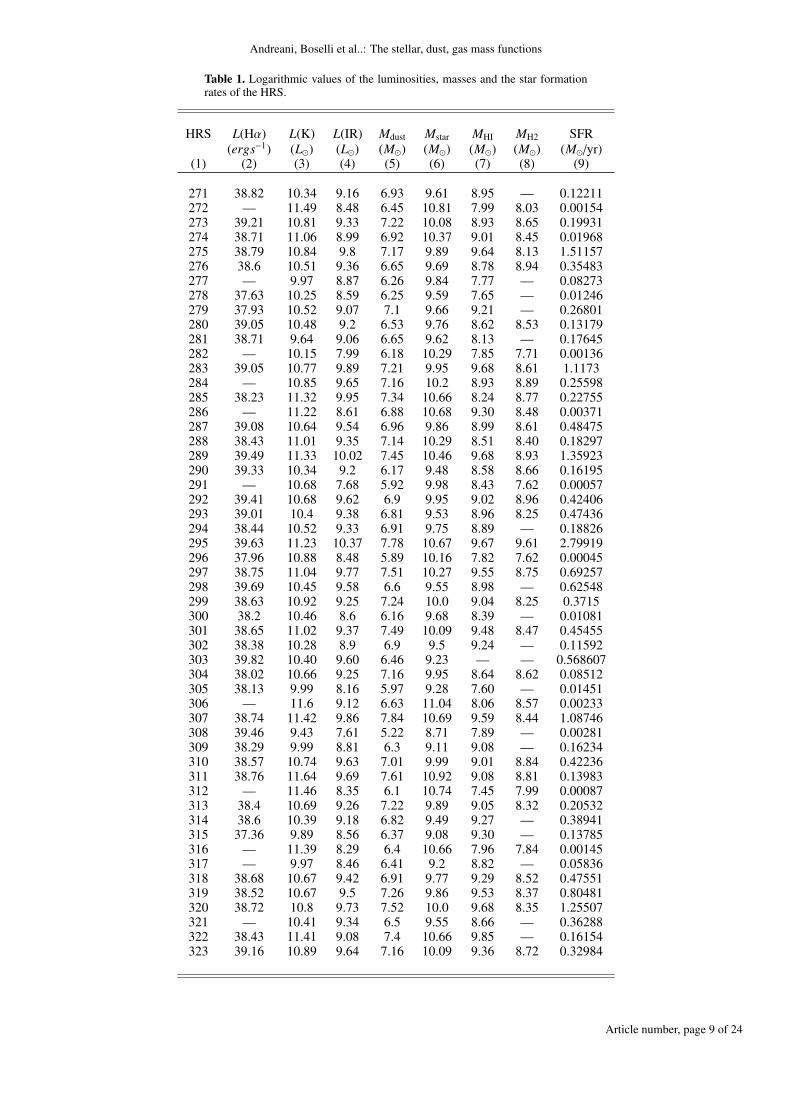
The first step in the above procedure is the estimation of themarginals. In absence of any a priori knowledge of the analyticalform of φ̂(x) and θ̂(y), a possible approach is represented by thesystem of three families, say SU, SB, SL, introduced by Johnson(1949) according to the fact that a random variable is unbounded(SU), bounded above and below (SB) or bounded only below(SL). A detailed description of such families as well of their usein practical application is given in Vio et al. (1994). Here, itis sufficient to say that the members of this system are charac-terised by four free parameters that allow them a great flexibilityin reproducing most of the classical PDFs. As described in Vioet al. (1994), a robust method to select the specific family andto estimate the corresponding parameters for a given set of datais based on the percentiles of their empirical distribution. In thepresent case, this method indicates the SB family

f (x) =η√

2π

λ

(x − ε)(λ − x + ε)exp−

{12

[γ + η ln

( x − ελ − x + ε

)]2}

(10)

with ε ≤ x ≤ λ + ε as the most suited to reproduce the PDF ofthe observed data. Table 2 shows the estimated parameters andFig. (1) the corresponding PDFs vs the experimental histograms.Finally, Figs (3)-(8) show the corresponding bivariate PDF ob-tained by means of Eq. (6).

It is important to stress here that, as explained in detail inAndreani et al. (2014), we have considered several PDFs tofit the K-band luminosities. All of them have a support of typeLmin < L < ∞ (or Mmin < M < ∞), a steep slope for L → Lmin



(or M → Mmin) and the possibility that φ(L), φ(M) → ∞. Butsince the Lmin (or Mmin) is unknown, the three-parameters ver-sion of such PDF has to be used. The fit of this kind of PDFs isa difficult problem since the maximum likelihood approach failsif φ(L), φ(M)→ ∞ when L→ Lmin (or M → Mmin).

This problem has been solved with the method described inAppendix A in Andreani et al. (2014).

4.1. Analysis of the bivariate LFs

Before discussing the outcomes of our analysis of the bivariatePDFs shown in Figs (3)-(8) we examine the distribution of thephysical quantities listed in Table 2 and plotted in Figure 2.

The green colours correspond to the galaxies classified asLT according to the classification in Cortese et al. (2012a),while blue to the ET1.

The same colour code is used in the diagonal inlayings whichcontain the histograms of the two populations. The first result isthat the histograms are quite distinct and clearly show in mostof the cases the existence of two distinct distributions for LTGsand ETGs. The two populations cover different values of lumi-nosities and masses. Atomic, molecular and total gas masses,infrared luminosities and SFR are much larger in LTGs, whilethe K-band luminosity and the stellar masses are larger in theETGs. The distribution of the dust mass is similar in LTGs andETGs, but the distribution is shifted to lower value in ETGs of0.5 dex. The relations among these variables are not affected bythe luminosity-distance relation, because the HRS is a volume-limited sample. The values of the correlation coefficients arelisted in the sixth column of Table 2.

The analysis of the correlations implies that a correct statisti-cal analysis for many physical quantities can only be carried overa subset of the sample: either containing only ET or only LT.We have then computed the bivariate functions over the wholesample only in one case (stellar mass) for which we cannot dis-tinguish the behaviour of the two populations. In the followingwe compute most of the bivariates for LTGs, and, because ofthe limited statistics, only the overall trends are discussed for theETGs in the sample.

Errorbars are computed with a bootstrap technique, itera-tively extracting the values of the marginal functions (see § 4above) when the variable changes within its errorbar.

4.1.1. The bivariate L(K) − Mstar

Both Figure 2 and the bivariate LF LK-Mstar in Figure 3 highlightthe tight relation between the K-band luminosity and the stellarmass (Gavazzi et al. 1996). The correlation coefficient is 0.965.This is not surprising as the stellar masses are derived from thei-band luminosity and g − i colour, close to the K-band (Corteseet al. 2012a; Boselli et al. 2009). Both ETGs and LTGs followthe same correlation, with the former objects containing largerstellar masses. A few sources can be identified both in Figure 2and Figure 3 as outliers because they deviate from the tight cor-relation. This deviation is clearly visible in Figure 3 where thevalues are on a linear scale.

The K-band magnitude of the HRS sample are taken fromthe 2MASS survey, these outliers may have not well derived val-

1 The original classification was a NED-based morphological typeclassification (Boselli et al. 2010a) which has been modifed for sev-eral galaxies after revision based on more recent literature and visualispection as discussed in Cortese et al. (2012a)

ues of the K-band mag due to their complex morphology andlow surface brightness (Kochanek et al. 2001), and closenessto the completion limit of the survey (Jarrett et al. 2000). In-deed, the errorbars on the photometry for the extended (and morenearby) and low surface brightness galaxies are more affected bysky fluctuations on large scale (see discussion in Appendix A inKochanek et al. 2001).

Overall this correlation confirms a well known result that theK-band mag is a fair tracer of the stellar mass. Figure 3 showsthe marginal function used to compute the bivariate in section 3representing the stellar mass distribution. This can be retrievedfrom the analytical form of equation (10) using the parameters inTable 2. Bearing in mind that a strict comparison with previousworks on the stellar mass function (SMF) of the local universe isnot straightforward because our different way of computing thisfunction, we draw in Figure 3 together with our derived marginalthe Schechter (Schechter 1976) functions whose parameters areextracted from the best fit of the SMFs by Baldry et al. (2012).These authors have characterised the SMF at z ∼ 0 down toM = 108M� using data from the GAMA surveys and fit theirdata with a double Schechter (Schechter 1976) function witha single value for the break mass, and provide a good fit to thedata for M > 108M�. They claim that this is approximately thesum of a single Schechter (Schechter 1976) function for the bluepopulation and double Schechter function for the red population.

The deviation of the marginal derived in this work with theSMFs computed by Baldry et al. (2012) at stellar mass lowerthan ∼ 3 × 109M� simply highlights the incompleteness of theHRS sample at low stellar mass, i.e. the lack of galaxies with lowstellar mass in the HRS sample. The HRS sample covers a smallvolume and lacks the necessary depth to detect K-band mag faintand/or low surface brigthness galaxies.The low end of the mass function is dominated by disc galaxies,i.e. the LTGs, (Thanjavur et al. 2016), which the HRS misses asdiscussed above.

The high-mass end of the SMF is in agreement among thedifferent samples and confirms previous findings that it is domi-nated by spheroidal galaxies. Thanjavur et al. (2016) show thatat masses lower than log(M/M�)=10.3 there is a preponderanceof disc galaxies, whereas increasing galaxy stellar mass, this discdominance gradually decreases with a corresponding increase inthe spheroidal contribution. Although the SMF of the disc com-ponents shows a steep increase at the faint end, their contributionto the total galaxy stellar mass density is only 37 per cent. Thisgradual change of the SMF from disc dominated to spheoridaldominated galaxies is linked to the physics and environmentalprocesses which drive the build-up of stellar mass in these twoprincipal galaxy components (Thanjavur et al. 2016). The lackof small disc galaxies could be also due to the environment andthis could be well the case for the HRS sample (Boselli et al.2014a, 2016). Changes on the shape of the local SMF (and in thevalue of M?) in the highest density environments, which containan enhancement of massive galaxies, are discussed in Blanton &Moustakas (2009).

4.1.2. The bivariate L(K) − L(IR)

The relation between the IR luminosity and the K-band lumi-nosity clearly highlights a dichotomy for the two morphologicaltypes (ET) and (LT), the relation is almost linear in logarithmicscale (L(K) ∼ α · L(IR), with α ∼ 10, 1000 for LT and ET re-spectively). The IR luminosity is fainter in ETGs, while LTGshave fainter values of the K-band luminosity. A closer look at theK-band/IR luminosity relation in Figure 2 shows that one tenth



Table 2. Coefficients of the PDFs of the SB family (eq. 10) for LTGs only and the whole sample

Variable η ε λ γ corrL(K) 0.6641 0.002039 2.658 2.521 1.000L(IR) 0.7509 -0.001622 8.233 2.705 0.790Mdust 0.7874 -0.000153 6.773 3.482 0.849Mstar 0.6974 0.003965 2.879 2.467 0.967SFR 0.6316 -0.001695 11.15 2.498 0.389MHI 0.6393 0.000966 2.519 2.277 0.431MH2 0.9067 0.007500 14.85 2.881 0.672Mb

star 0.6270 0.004132 8.343 2.682 0.965

b computed over the whole sample

of the objects have properties in between the relations definedfor ET and LT respectively. The majority of these objects host aweak AGN and/or are classified as ’retired galaxy’ by Gavazziet al. (2018). These galaxies have been star-forming in the pastand, although the nucleus is sterilised, there are still remnants ofstar formation in the outer region. They share most of the prop-erties of the ETGs, with less gas and very low specific SFR. Thelower left part of the L(K) − L(IR) plane is occupied mosty byobjects classified as LTGs dominated by HII regions (Gavazzi etal. 2018).

Because of the low number of ET objects and the distinctbehaviour of the ET and LT galaxies with respect to the IR Lu-minosity, Figure 4 shows the BLF for LTGs only. In spite ofthe relative good correlation measured (0.79) the BLF shows aspread at large values of the IR and K-band luminosities. The ob-jects responsible for this spread are galaxies of the Virgo Clusterand host a weak AGN and/or are classified as ’retired galaxy’ byGavazzi et al. (2018). These objects might be in migration fromthe blue cloud (star-forming) to the green valley (post-starburst)and eventually to the red sequence. Particulary those in the Virgocluster loose gas (mainly atomic) through ram pressure strippingand have more compact discs because of the further loss of dustand molecular gas (Boselli et al. 2014c, 2016).

In Andreani et al. (2014) a similar BLF has been computedlimited to the monochromatic luminosities in the far-IR (in theS PIRE bands at 250, 350 and 500µm). Andreani et al. (2014)discussed how for LTGs the dependence L(K) − L(IR) can beinterpreted as a physical connection between the cold componentof the dust – closely related to the galaxy dust mass – and thestellar mass – inferred from the K-band absolute luminosity –which is a tracer of the mass of the old stellar population.Figure 4 shows the analytical form (the marginal) computed insection 3 of the local IR luminosity function. To locate this find-ing in the context of other authors’ results, Figure 4 reports thebest fit of the modified Schechter function derived by Marchettiet al. (2016) using the Herschel HerMES survey. This latteris the most recent version of the local IRLF based on blindFIR/submm surveys (Vaccari et al. 2010; Negrello et al. 2013;Clemens et al. 2013; Wang et al. 2016) and computed using thetotal far-IR (3-1000µm) luminosity combined with models.

The agreement shown in Figure 4 is good with small devia-tions at low and large luminosities. While at large luminositiesthe HRS is statistically not complete because of the small sur-veyed area, the discrepancy at low IR luminosities can be at-tributed to the ways these samples have been selected: the HRSsample is a K-band selected and may miss very low IR lumi-nosity objects which are more easily detected in blind FIR sur-veys. There might be an additional factor related to the defi-nition of morphology/colour in the infrared and in the optical.

Marchetti et al. (2016) interpret the shape of the local far-IR LFas due to the contributions of red (possibly ET) and blue (possi-bly LT) galaxy populations, with their different Schechter forms,rapidly evolving already at low redshifts. However, the cut-offline between red and blue galaxies in this context is less sharpthan in the optical classification of the galaxy morphology, as inthe HRS sample, where among red galaxies there are red spiralgalaxies that could be the result of their highly inclined orien-tation and/or a strong contribution of the old stellar population(see also Dariush et al. 2016).

4.1.3. The bivariate Dust Mass Function (DMF),L(K) − Mdust, and the relation Mdust − Mstar

As shown in Figure 2 the variation of the K-band luminosityin ETGs is roughly constant with respect to the dust mass, and,considering also the upper limits, there is no correlation betweenthe star luminosity and the dust emission. For this reason andfor the low statistical significance of the number of ETGs wecompute the bivariate PDF LK − Mdust shown in Figure 5 onlyfor LTGs. The dependence of the K-band luminosity and the dustmass shows a very tight relation, with a correlation coefficient of0.849, slightly stronger than that between L(K) − L(IR). This isexpected as the dust thermal emission is the main contributor ofthe IR luminosities.

Stellar and dust masses seem to be in tight relationship,which could be interpreted as a relationship among the stel-lar mass, the cold dust mass, and the far-infrared luminosity inLTGs. This tightness can alse be due to the presence of old starswhich dominate the stellar mass and at the same time produc-ing the dust in their stellar winds (Dwek 1998; Zhukovska et al.2008, 2016). What is clear is that the distribution of the cold dustin the galaxy discs follows that of the stars.

The spread of this relation, due to the objects with largerdust mass and low K-band luminosity (small stellar mass), canbe ascribed to the fact that lower (stellar) mass galaxies havehigher dust mass fractions than their more massive counterparts(Cortese et al. 2012b; Clemens et al. 2013).

From this function, using equation (10) and Table 2, we canderive the DMF which is shown in Figure 5. In the same figurewe plot the DMFs obtained by Dunne et al. (2011), the best-fistmodel by Clemens et al. (2013) and the recent one by Beeston etal. (2017). Dunne et al. (2011) and Beeston et al. (2017) com-pute the DMF over a sample of Herschel selected galaxies, whileClemens et al. (2013) over a sample selected from the Plancksource catalogue. Clemens et al. (2013) claim agreement withthe Dunne et al. (2011) values because of the large uncertaintieson the derivations of the dust masses, which are mainly linked tothe assumed physical properties of the dust (see also De Vis et



al. 2017). All these models make use of SED fitting templatesto derive the physical parameters of the galaxies (therefore alsothe value of the dust mass). The mostly used MAGPHYS pack-age (Clemens et al. 2013; Beeston et al. 2017; Driver et al.2018) combines black bodies with different temperatures, keep-ing the energy balance between UV/optical and NIR while forHRS Ciesla et al. (2014) fitted the Draine and Li models onlyon the IR part.Although the accuracy of the dust mass values mainly dependson the quality of the fit (i.e. the number of photometric points), itis also largely depending on the dust model, which assumes dustabsorption coefficient differing up to a factor of two, among thedifferent models Other uncertainties may arise from the selectioncriteria and systematics which are not perfectly under control.

To overcome some of the discrepancies we make use of therecomputed values reported in Beeston et al. (2017) who haverescaled the DMFs at the same value of the dust absorption co-efficient. These rescaled DMFs are those shown in Figure 5.

The DMF computed for the HRS sample lies in between theDMF given by Clemens et al. (2013)’s and those derived byDunne et al. (2011); Beeston et al. (2017). We do not wantto overinterpret this result because of the difference on the dustmodels, the difference in the selection wavelengths (250µm and500µm), and in the catalogues (Herschel/SPIRE and Planck).We can claim that the Local DMF derived from the HRS isconsistent with the values found for far-IR/submm galaxies. Weneed to keep in mind, however, that the HRS may miss a numberof dusty galaxies because it targets K-band selected objects.

Herschel galaxy samples contain red galaxies which maycorrespond to the optical classification of both LTGs and ETGs(i.e. contain part of the ETGs of the HRS sample), withdust masses similar to the blue objects, i.e. normal spiral/star-forming systems. Some red ETGs keep the properties of opti-cal ETGs (lower mean dust-to-stellar mass ratios, lower meanstar-formation / specific-star-formation rates) but a populationof ETGs exists, containing a significant level of cold dust simi-lar to those observed in blue/star-forming galaxies. The origin ofdust in such ETGs it is still unclear. It could be of external origin(e.g. fuelled through mergers and tidal interactions, Dariush et al.(2016)) or long lived in galaxy discs, with late results favouringthis latter interpretation (Bassett et al. 2017), (see also Gomezet al. 2010; Cortese et al. 2012b; Smith et al. 2012; Agius et al.2015; Eales et al. 2018).

The tight relation between the K-band luminosity and thestellar mass (see Figure 2 and in Figure 3) allows to explore aswell the relation between the dust and the stellar masses. Thislatter is very tight for the LTGs, while no clear connection is de-tected in ET objects. This is expected as about half of the ETGsremain undetected in the Herschel bands (Cortese et al. 2012b;Smith et al. 2012), the corresponding IR luminosity and deriveddust masses have to be considered as upper limits (Ciesla et al.2014).

Cortese et al. (2012b) show that the spread in the relationbetween stellar and dust masses in the HRS may be attributed tothe variation of the dust content as a function of the environmentand of the HI content more than to the morphological (late versusearly) type.

4.1.4. The bivariate L(K)-SFR

The SFR BLF is displayed in Figure 6. The computed bivariatefunction shows a slight relation between the SFR and the K-bandluminosity, with this latter, as highlighted in Figure 2 and in Sec-tion § 4.1.1 strongly linked to the stellar mass.

Figure 6 displays the SFR functions derived in this workfrom the BLF and compares it with the values obtained fromother samples. The comparison is not straightforward becauseof the way the SFR has been computed in the different samples.The HRS SFR is the average value among that derived from thedust corrected Hα luminosity, the far-UV dust corrected lumi-nosity and the radio emission at 20cm (Boselli et al. 2015). SFRvalues in other samples have been obtained either from the Hαmeasurements alone (Bothwell et al. 2011; Gunawardhana et al.2013) or translating the IR luminosity to SFR (Clemens et al.2013).

It is straightforward to see that the SFR function is a strongfunction of the sample selection criteria. While the SFR functionextracted from the Hα is significantly lower than that computedfrom the IR luminosities the behaviour of the HRS SFR functionmisses large values of the SFR.

We are not at all astonished to see a large difference athigh star formation rates with the Planck derived Clemens et al.(2013)’s LF, which includes FIR selected starbursts known to betotally absent in the local universe (within 25 Mpc the most ex-treme case is M82, with ∼10M�/yr) and might be limited/biasedby confusion. Furthermore, the difference in the several pub-lished Hα selected SFR LF is huge (see Fig. 11 Boselli et al.2015), even within the same work once different samples areused. Gunawardhana et al. (2013) published two different SFRLFs derived from Hα, one from SDSS data, the second one fromGAMA data, which is higher at least at low SFR values. Boselliet al. (2016) have compared these Hα LF (GAMA and SDSS) tothe one derived using NUV data in the Virgo clusterv peripheryand they match pretty well. This means that the observed dif-ferences in the SFR LF between HRS and Gunawardhana et al.(2013)’s are mainly due to the sample, and not to the method toderive SFR.

In the past two decades a vast number of works have investi-gated the link between the SFR and the stellar mass (i.e. Eales etal. 2017, and references therein). Our interpretation of the SFRbivariate function is that the relation between the SFR and Mstaris a combination of at least two factors. On the one hand, thereis an effect due to the environment. Boselli et al. (2016) link thedecrease in the star formation activity in the main sequence re-lation to HI-deficiency, which may be due to ram pressure strip-ping (Boselli et al. 2015, 2016). The location of the galaxy mainsequence is different for objects which do show sign of perturba-tion from that drawn by unperturbed systems. Many of the HRSgalaxies show sign of perturbation due to the environment and alarge infall rate of star forming systems is observed in Virgo.

On the other hand, there is a selection effect. The HRS sam-ple contains most of the stellar mass in a specific volume of lo-cal Universe and, as discussed above in § 4.1.3, it should notbe biased towards galaxies with high star formation rates. Butit contains optically classified red galaxies that are red not onlybecause of the old stellar population but because of a fraction ofdust and gas which show that they are still forming stars. 30%of the red population classified as ET still contains a fraction ofdust and have a residual star formation rate (Eales et al. 2017).For very red objects, those with the lowest values of the SFR theredness is due to an old population and not to dust reddening andthe values of the ratio Mdust

Mstarare < 10−4.

We are not able to investigate further this issue using theBLF. The number of objects is low to split the sample and com-pute the BLF differently on the galaxies belonging to the clusterand those of the fields.



4.1.5. The bivariates L(K) − Mgas, atomic and molecular gas

In Figures 2, 7, 8, we report the values of the distributions of theatomic gas, and the molecular gas masses and the bivariate massfunctions. The amount of atomic and molecular gas is a strongfunction of the morphological type, where most of the ETGs areundetected in atomic and molecular gas (Boselli et al. 2014a).

The derived atomic gas function for LTGs only and thoseobtained by HI dedicated surveys (Zwaan et al. 2005; Martin etal. 2010; Hoppmann et al. 2015; Jones et al. 2018) are shownin Figure 7. Overplotted are also the predictions by Popping etal. (2014) and Lagos et al. (2011). The M(HI) − MF derivedfrom the HRS data differs substantially at values M(HI) > a few×109M�. The weak correlation of the HI mass with the K-bandluminosity (see Figure 7a and Table 2) does not allow to stronglyconstrain the bivariate and as a consequence the construction ofthe atomic gas mass function is poorly determined. This mayexplain the strong difference in shape observed in the HI MF.

The deficiency of large mass objects can be explainedtwofold: the HRS is a K-band luminosity selected, while theHI dedicated surveys are blindly selecting HI emitting galaxies(Zwaan et al. 2005; Martin et al. 2010; Hoppmann et al. 2015;Jones et al. 2018). The HRS sample therefore may miss mostof the HI-massive galaxies. Secondly, the HRS contains moreHI deficient objects as normal field galaxies (roughly half of thesample). This fact is attributed to the presence of the Virgo clus-ter and its gravitational effect on the gas. Through direct strip-ping of the ISM from the disc (e.g., ram pressure) the galaxydisc looses its atomic gas content as widely discussed in the var-ious HRS follow-up papers (Boselli et al. 2014c; Cortese et al.2016).

At variance with the HI mass the BLF of the H2 mass isrelatively strong correlated with the K-band luminosity (see Fig-ure 8 and Table 2). The correlation shown in Figure 8 reflectsthe relation between the stellar mass and the molecular gas masswithin the sample with the scatter due to the HI-deficient galax-ies (Boselli et al. 2014b). Boselli et al. (2014c) have used theM(H2) versus stellar mass, Mstar, scaling relation to define theH2-deficiency parameter as the difference, on logarithmic scale,between the expected and observed molecular gas mass for agalaxy of given stellar mass. This molecular hydrogen deficiencyis considered as a proxy for galaxy interactions with the sur-rounding cluster environment. The molecular gas and the exten-sion of the molecular disc are also affected by the presence ofthe cluster galaxies and on average these galaxies have a lowermolecular content than galaxies in the field. A similar findingis reported by Fumagalli et al. (2009) who find that moleculardeficient galaxies form stars at a lower rate or have dimmer farinfrared fluxes than gas rich galaxies, as expected if the star for-mation rate is determined by the molecular hydrogen content.A different view has been proposed by Mok et al. (2016) whoargue that Virgo galaxies have longer molecular gas depletiontimes compared to group galaxies, due to their higher H2 massesand lower star formation rates and suggest that the longer de-pletion times may be a result of heating processes in the clusterenvironment or differences in the turbulent pressure. This issuerequires further studies and is not settled yet.

Figure 8 displays the H2 MF derived from the BLF (Fig-ure 8) compared with the predictions by Lagos et al. (2011).At masses lower than 108M� the HRS sample may miss galax-ies with low content of molecular hydrogen. However, very fewsamples in the Local Universe are complete in molecular hydro-gen and the data of galaxies with very low molecular contentin unbiased samples are still scanty (i.e. Bothwell et al. 2016).

Previous molecular MFs of nearby galaxies have been derivedfrom the CO MF. Keres et al. (2003) used an incomplete COsample based on a far-IR selection and exploiting the correlationwith the 60µm luminosity. The resulting CO MF is, therefore,biased towards gas rich galaxies. An updated estimate of the H2MF, based on an empirical and variable CO-H2 conversion fac-tor, was presented by Obreschkow and Rawlings (2009). Weuse in Figure 8 the molecular mass function derived from theL′(CO) luminosity distribution of Saintonge et al. (2017) fromthe COLD GASS (CO legacy data base for GASS; Saintongeet al. (2011)) survey. This last survey, although biased towardsmassive galaxies (stellar mass, Mstar > a few 109M�, Saintongeet al. (2011, 2017)), i.e. it might not sample a sufficiently largedynamic range in Mstar to trace a fair distribution, is at present theonly survey with a large enough database to allow a fair recon-struction of the L′(CO) luminosity distribution. However, thissample too is not unbiased, i.e. it is not CO-selected.

The comparison shown in Figure 8 of the molecular massfunction derived from the HRS and that from the COLD GASSsample is only indicative. In addition to the issues discussedabove we lack the information about the galaxy properties to ap-ply the luminosity dependent conversion factor between L′(CO)and M(H2) equal to the one used by Boselli et al. (2014b). Whatwe show in Figure 8 is our derived H2 MF using a constant con-version factor (αCO = 3.6M�/(Kkms−1pc2). Moreover, the com-pleteness at low molecular masses is for both samples very poorand below log(M(H2)) = 8.4M� nothing can be inferred.

5. Discussion

The fundamental goal for theoretical models of galaxy formationand evolution is reproducing the observed statistical distributions(such as LFs, stellar and cold gas MFs) of the global propertiesof the galaxy populations at different cosmic epochs.

On the one hand, most of the models are not able to recon-struct the whole spectrum of data, commonly used to fix theparameters, and to predict the evolution at larger redshifts. Be-cause of the large uncertainties in the theory associated with thephysics of the SF, stellar and AGN feedback and environmentaleffects, key is tuning the multi-parameter space by fitting the ob-served physical properties of the galaxies in the Local Universe.In addition, many free parameters are frequently degenerate witheach other, and the tuned recipes make these models more or lesssuccessful in predicting the galaxy evolution over cosmic time.

On the other hand, from the observational side, the buildingup of samples sufficiently large to be statistically meaningful andwith a wide wavelength range to cover the whole spectrum ofobserved properties is laborious. But this would be the only wayto allow a fair comparison with models and to keep biases andsystematics fully under control.

We have discussed extensively the limitations of the HRSsample and constrained its biases and selection effects while dis-cussing the individual mass and luminosity functions. The sam-ple is strongly limited in statistical significance by the smallnumber of sources which does not allow to fully constrain theproperties of the various functions. However, it is the only lo-cal sample which has a large coverage in wavelengths for whichmany physical properties can be simultaneously studied. Thelarge number of observations and the original well defined se-lection in the K-band have been used to define several LFs andMFs presented in this work which can be used to constrain thegalaxy formation models.

At a first order, the BLF and BMF that we estimate are fairlycomparable to those derived in the literature given the wide va-



riety of functions published not always consistent one another.Just for an example, the SFR LF seems to be the most differentfrom those derived in the literature.

It is clear that the SMF and the atomic gas MF, are very welland better determined in much larger local samples, but in thecases as the dust and the molecular MF, for which data are eitherscanty or not well constrained, the functions determined fromthe HRS show good quality and at the same level or even betterthan those found in the literature.

Furthermore, the HRS is composed of galaxies located in awide range of environments, from the general field to the coreof the Virgo cluster, the largest concentration of galaxies in thenearby Universe. It is thus ideally defined to study in great de-tail environmental effects on the different galactic components(stars, gas, dust). Thanks to its proximity (∼ 20 Mpc) and to thequality of the multifrequency data gathered so far, this sampleis a unique laboratory for studying the role of mass and environ-mental quenching and feedback on galaxy evolution down to subkpc scales.

5.1. The local LFs, the IR luminosity and the SFR densities

The IR LF derived from the bivariate PDF LK-LIR is well inagreement with that extracted from blind far-IR survey, it de-viates mainly at low-IR luminosity where the HRS likely misseslow luminosity galaxies. The selection in the K-band, as dis-cussed in § 4.1.2, may miss low surface density objects, faintoptical galaxies and galaxies with IR luminosity larger than thatexpected for a given K-band luminosity. Overall the agreementwith the caveats mentioned above is good.

The present derivation of the luminosity functions allow usto derive the local extragalactic luminosity density. This latter iscomputed integrating the functional form of the LFs within thelimits where the function is defined L(IR) = 2×108÷6×1010L�.The density of the IR luminosity in the local Universe, mea-sured from the HRS IR LF shown in Figure 4 turns out tobe 1.5 107L�Mpc−3, a factor five lower than that reported inMarchetti et al. (2016), 8.3 107L�Mpc−3. The HRS misses star-burst galaxies because of the small sampled volume.

The SFR function derived from the bivariate PDF LK-SFR asdiscussed in § 4.1.4 shows a very different behaviour from thosederived from Hα surveys and from blind IR surveys mainly atlarge values of the SFRs. This reflects two problems. First, thelarge difference in sampling the local SFR from optical and IRsamples and secondly the inference of the SFR from the observ-ables with the optical values which are largely affected by theuncertainties on the attenuation correction factors. These latterdepend on parameters such as stellar mass and dust temperature,and our poor understanding of the relation between the IRX ra-tio (L(IR)/L(UV)) and the UV spectral slope (see for extensivediscussion, Wang et al. 2016).

Likely because the HRS SFR function misses large valuesof the SFR, due to the lack of starburst galaxies, the local SFRdensity computed on this sample is a factor of two below thatdetermined from other local surveys. The SFR density is inferredintegrating the derived SFR function shown in Figure 6 (withinthe integration limits S FR = 0.01÷15M�/year) and turns out tobe (1.6 ± 0.4)10−3M� yr−1 Mpc−3 which is a factor 2 lower thanthat derived from other optical (Gunawardhana et al. 2013) and5-10 times lower than that derived from IR suverys (see Clemenset al. 2013; Marchetti et al. 2016, and reference therein). Thisis not surprising as a large scatter in the local SFRD estimatesusing different SFR diagnostics is seen. In addition galaxies inthe Virgo cluster show a reduced SFR. The Hα measurements

present the largest scatter among different published results (seeFigure 11 in Boselli et al. 2015), (Marchetti et al. 2016, andreference therein).

5.2. The local mass functions and local mass densities

As discussed in section 4.1.1 the SMF of the HRS shows adeficit of small galaxies due to the limit in the original se-lection in the K-band and to the poor sampling of low sur-face brightness galaxies. The computed local stellar mass den-sity of the HRS (integrating the functional form over the rangeMstellar = 109 ÷ 2 × 1011M�) turns out to be 2.25 108M� Mpc−3,within a factor of 2 from that computed integrating the best fit ofthe SMF given by Baldry et al. (2012).

The dust mass function of the HRS sample follows closelythe same behaviour as those derived from other blind IR surveys.The large scatter shown among the different functions reflect theuncertainties related to the physical and chemical properties ofthe dust grains. The derived local dust mass density has a valueconsequently in between the value derived with the Dunne etal. (2011); Beeston et al. (2017)’s and Clemens et al. (2013)’smass functions. The dust mass local density ∼ 8 104M� Mpc−3,obtained integrating the functional form (Eq. 10) over the range105÷5 108M�, agrees within the uncertainties with those derivedfrom the other DMFs computed so far and rescaled by Beeston etal. (2017) at the same value of the dust absorption coeffecient, ∼1.5 105M� Mpc−3. Driver et al. (2018) report from their analysison the GAMA survey an average value of the local dust massdensity of ∼ 1.4 105M� Mpc−3.

Figure 7 shows the atomic gas function and highlights thatHI-MF derived from the HRS data differs substantially at val-ues M(HI) > a few ×109M�. This is due to the very weak cor-relation between the HI mass with the K-band luminosity (seeFigure 7 and Table 2) which does not allow to strongly constrainthe bivariate and as a consequence the construction of the atomicgas mass function is poorly determined. In particular we find adeficiency of large mass objects in the HRS survey because itsselection in the K-band misses galaxies with large values of theatomic gas found in HI dedicated blind surveys (Zwaan et al.2005; Martin et al. 2010; Hoppmann et al. 2015; Jones et al.2018). Moreover, the HRS contains more HI deficient objectsthan normal field galaxies, due to the presence of the Virgo clus-ter, and the likely direct stripping of ISM from the disc (e.g., rampressure) (Cortese et al. 2016; Boselli et al. 2014c).

The molecular mass function reported in Figure 8 is the firstfunction built on a complete sample, although the completenessis in the K-band. The H2 mass is relatively strong correlated withthe K-band luminosity due to relation between the stellar massand the molecular gas mass within the sample with the scatterdue to the HI-deficient galaxies. The derived H2 MF when com-pared with the predictions by Lagos et al. (2011), shows a deficitat masses lower than 108M� where the HRS sample may missgalaxies with low content of molecular hydrogen.

We have derived a very rough molecular mass function fromthe best-fit of the CO luminosity distribution by Saintonge et al.(2017) and compare this function to the one computed over theHRS sample. The comparision is only indicative. It shows over-all good agreement but at small molecular mass where neitherthe HRS nor the COLD GASS sample are complete and there-fore we cannot infer any meaningful conclusion. The molecularmass local density turns out to be 107M�Mpc−3.

Table 5.2 summarises the values of the local luminosity andmass density derived from our analysis.



Table 3. local luminosity and mass densities

Luminosity/Mass Local density value

IR luminosity 1.5 107L�Mpc−3

SFR 1.6 × 10−3M� yr−1 Mpc−3

Stellar mass 2.25 108M� Mpc−3

Dust mass 8 104M� Mpc−3

Molecular mass 107M�Mpc−3

6. Conclusions

The construction of the LFs and the MFs has made possible us-ing the bivariate based on the K-band selection. We have dis-cussed the LFs and MFs derived from the HRS and comparedwith the same LFs and MFs derived from local samples selectedin complete different ways. This comparison highlights the limitsand biases inherent to the HRS but also its strength as represen-tative sample of the Local Universe.

The analysis shows that the behaviour of the morphologi-cal (optically selected) subsamples is quite different and a sta-tistically meaningful result can be obtained over the whole HRSsample only from the relationship between the K-band and thestellar mass. The same analysis with the other physical quantities(dust and gas masses, far-IR luminosity and star formation rate)has to be restricted to the late-type galaxy (LTG) subsample. TheLFs, MFs of LTGs are generally dependent on the K-band andthe various dependencies are discussed in detail. We are able toderive the corresponding LFs and MFs and compare with thosecomputed with other samples and with results from galaxy for-mation simulations.

The analysis reported in this paper represents a fundamen-tal local benchmark to compare with models of galaxy evolu-tion. The HRS is designed to provide a concise view of the largegalaxies in our local Universe. The results found in this workcould therefore be representative for late type galaxies. The de-rived relations can be applied to a larger set of local galaxies andcan be compared with a similar analysis at higher redshift.Acknowledgements. This research has made use of data from the HRSproject. HRS is a Herschel Key Programme utilising guaranteed time fromthe SPIRE instrument team, ESAC scientists and a mission scientist. TheHRS data was accessed through the Herschel Database in Marseille (HeDaM- http://hedam.lam.fr) operated by CeSAM and hosted by the Laboratoired’Astrophysique de Marseille. We acknowledge financial support from Pro-gramme National de Cosmologie and Galaxies (PNCG) of CNRS/INSU, France.Parts of this research were conducted by the Australian Research Council Centreof Excellence for All Sky Astrophysics in 3 Dimensions (ASTRO 3D), throughproject number CE170100013. P.A. warmly thanks Ken Tatematsu-san for hiskind invitation to Japan and his hospitality at the Nobeyama Observatory. Shewarmly thanks NAOJ-Chile for her stay at Mitaka where this work has beencompleted. We thank an anonynous referee whose help has largely improved thereadability of the paper

ReferencesAgius N.K. et al., 2015, MNRAS 451, 3815Andreani P., Spinoglio L., Boselli A., Ciesla L., Vio R., et al.., 2014 A&A 566,

70Baldry I. K., 2012, MNRAS 421, 621Bassett R., et al., 2017, MNRAS 470, 1991Beesen R.A et al., 2017, arXiv:1712.07261Bendo G. et al. 2012, MNRAS 423, 197Binggeli B.A. , Sandage A., Tamman, G.A., 1988 ARA&A 26, 509BBlanton M.R., et al., 2001 AJ 121, 2358B

Blanton M.R., & Moustakas J., 2009, Ann. Rev. Astron. Astroph. 47, 159Bell E.R.. et al., 2003 ApJS 149, 289BBoselli A. , Gavazzi G., 2006, PASP 118, 517Boselli A. , Gavazzi G., 2014, A&A 570, 69Boselli A. et al.., 2009, ApJ 706, 1527Boselli A. et al.., 2010a, PASP 122, 261Boselli, A., Boissier, S., Heinis, S., et al.. 2011, A&A, 528, A107Boselli A., Hughes, T. M., Cortese, L., Gavazzi, G., and Buat, V. 2013, A&A

550, 114Boselli A., Cortese L., Boquien M., 2014a A&A 564, 65Boselli A., Cortese L., Boquien M., Boissier S., Catinella B., Lagos C., Saintonge

A. 2014b A&A 564, 66Boselli, A.; Cortese, L.; Boquien, M.; Boissier, S.; Catinella, B.; Gavazzi, G.;

Lagos, C.; Saintonge, A., 2014c, A&A 564, 67Boselli, A. et al., 2014d, A&A 570, 69Boselli A., Fossati M., Gavazzi G., Ciesla L., Buat V., Boissier S., Hughes T. M.

2015 A&A 579, 102Boselli A., Roehlly, Y., Fossati, M., Buat, V., Boissier, S., Boquien, M., Bur-

garella, D., Ciesla, L., Gavazzi, G., Serra, P. et al., 2016, A&A 596, 11Bothwell M.S. et al., 2011, MNRAS 415, 1815Bothwell M.S. et al., 2016, MNRAS 455, 1156Ciesla L. et al.., 2012, A&A 543, 161Ciesla L. et al.., 2014, A&A 565, A128Ciesla L. et al., 2016, A&A 585, A43Clemens M.S. et al.., 2013, MNRAS 433, 695Cole S., et al.., 2001, MNRAS 393, 681Cortese L., et al.., 2010, A&A 518, L49Cortese L., et al.., 2012b, A&A 544, 101Cortese L., et al.., 2012a, A&A 540, 52Cortese L., et al.., 2014, MNRAS 440, 942Cortese L., et al.., 2016, MNRAS 459, 3574Dariush A., et al., 2016, MNRAS 456, 2221Davé R., et al., 2017, MNRAS 467, 115Davidzon et al.., 2016 A&A 586, A23De Vis P., et al., 2017, MNRAS 471, 1743Dressler A., 1980, ApJ 236, 351Driver S., et al., 2018, MNRAS 475, 2891Dunne L. , 2011, MNRAS 417, 1510Dwek E., 1998 ApJ 501, 643Eales S., et al., 2017, MNRAS 465, 3125Eales S., et al., 2018, MNRAS 473, 3507Fumagalli M., et al., 2009, ApJ 697, 1811Gavazzi G., Pierini, D. & Boselli, A., 1996, A&A 312, 397Gavazzi G., et al., 2018, in pressGomez H. L. et al., 2010, A&A, 518, 45Gunawardhana M. L. P. et al., 2013, MNRAS 433, 27641Hill D.T., et al. 2010, MNRAS 404, 1215HHoppmann L., Staveley-Smith L., Freudling W., Zwaan M.A., Minchin R.F., Cal-

abretta M.R., 2015, MNRAS 452, 3726Jarrett T.H., et al., 2000, AJ 119, 2498Johnson, N.L. 1949, Biometrika, 36, 149Johnston R., 2011, A&ARv 19, 41Jones M.G., Haynes M.P., Giovanelli R., Moorman C., 2018, arXiv:1802.00053Keres et al, 2003, ApJ 582, 659Kochanek C.S., Pahre M.A., Falco E.E., Huchra J.P., Mader M., Jarrett T.H.,

Chester T., and Cutri R., Schneider S.E. 2001, ApJ 560, 566Lagos C. del P., et al., 2011, MNRAS 418, 1649Lagos C. del P., et al., 2016, MNRAS 459, 2632Marchetti L., et al.., 2016, MNRAS 456, 1999Martin A.M., et al., 2010, ApJ 723 , 1359McKinnon R., Torrey P., Vogelsberger M., 2016, MNRAS 457, 3775Moustakas J., Coil A.L., Aird J. et al., 2013, ApJ 767, 50Mok, A., Wilson, C. D., Golding, J., Warren, B. E., Israel, F. P. et al., 2016

MNRAS 456, 4384



Negrello M., 2013, MNRAS 429, 1309Obreschkow & Rawlings, 2009, MNRAS 394, 1857Popping G. et al., 2014, MNRAS 442, 2398Saintonge A. et al, 2011, MNRAS 415, 32Saintonge A. et al, 2017, ApJS 233, 22Schechter, P., 1976, ApJ 203, 297, 1976Schlegel, D.J., Finkbeiner, D.P., Davis M., 1998 ApJ Supplement 500, 525Schmidt T., in Copulas: From Theory to Application in Finance, Jörn Rank (Ed-

itor), published by Risk Books, 2007Shankar F., Lapi, A., Salucci, P., De Zotti, G., Danese, L., 2006 ApJ 643, 14Smith D. J. B., Dunne L., da Cunha E., Rowlands K., Maddox, S. J., Gomez

H. L., Bonfield D. G., Charlot S., Driver S. P., Popescu C. C., et al., 2012MNRAS 427, 703

Takeuchi T. T. 2010, MNRAS 406, 1830Thanjavur, Karun; Simard, Luc; Bluck, Asa F. L.; Mendel, Trevor, 2016, MN-

RAS 459, 44Trivedi P.K., & Zimmer D.M. 2005, Copula modelling: an introduction for prac-

titioners, now Publishers Inc., Hanover: USAVaccari M. et al.., 2010, A&A 510, 20Vio R., Fasano, G., Lazzarin, M., & Lessi, O. 1994, A&A, 289, 640Wang L., et al., 2016 A&A 592, L5Zibetti S., Charlot S., Rix H.-W. 2009, MNRAS 400, 1181Zhukovska S., Gail H.-P., Trieloff M., 2008 A&A 479, 453Zhukovska S., et al., 2016, ApJ 831, 147Zwaan M., et al. 2005, MNRAS 359, L30



0 0.5 1LK (# 1e+12)

0

5

10

15

Prob

abilit

y D

ensi

ty

SB

0 2 4LIR (# 1e+10)

0

0.5

1

1.5

2

2.5

3

3.5

Prob

abilit

y D

ensi

ty

SB

0 1 2 3MDust (# 1e+08)

0

2

4

6

8

Prob

abilit

y D

ensi

ty

SB

0 0.5 1 1.5LH, (# 1e+40)

0

5

10

15

Prob

abilit

y D

ensi

ty

SB

0 1 2MStar (# 1e+11)

0

2

4

6

8

10

Prob

abilit

y D

ensi

ty

SB

0 0.5 1MHI (# 1e+10)

0

2

4

6

8

10

12

Prob

abilit

y D

ensi

ty

SB

Fig. 1. Histograms of the data in table 2 and corresponding fitted Johnson PDF. In all cases the SB family has been selected. The best fit parametersof the equation 10 are reported on Table 2. These PDFs have been used to estimate the bivariate PDF shown in Figures (4)-(6).


Andreani,B

osellietal..:The

stellar,dust,gasm

assfunctions

8 9 10Log(MGas)

8 9Log(MHII)

8 10Log(MHI)

10Log(MStar)

38Log(LH,)

6 8Log(MDust)

8 9 10Log(LIR)

10 11 12Log(LK)

8

9

10

Log(MGas)

8

9

Log(MHII)

8

10

Log(MHI)

91011

Log(MStar)

373839

Log(L H

,)

6

8

Log(MDust)

8910

Log(L IR)

10

11

12

Log(L K)

10 11#####12##########8######9#####10#############6###############8#######37#######38#########39###9########10###########11#### 8############10######

Log(LK) Log(LIR) Log(Mdust) Log(LH!) Log(Mstar) Log(MHI) Log(MH2)

Log(M

H2)

Number#of#galaxies

Number#of#galaxies

Number#of#galaxies

Number#of#galaxies

Number#of#galaxies

Number#of#galaxies

Number#of#galaxies

Fig. 2. Scatterplots and histograms for the data. Blue dots correspond to the objects with morphological type < 3 (ET ), green dots to objects with morphological type ≥ 3 (LT ). Because of the lackof data at some wavelengths the various panels contain a different number of points.

Article

number,page

19of24


5e8 1e9 2e9 5e9 1e10 2e10 5e10 1e11 2e11M stellar (solar mass)

1e -5

1e -4

0.001

0.01

0.1

Stel

lar M

ass

Func

tion

(1/M

pc3/

dex)

1 0

2 0

3 0

; = 0.965

2 4 6 8 10 12 14 16LK #1011

0.5

1

1.5

2

2.5

3

3.5

4

4.5

5

MStar

#1011

1 2 3 4#1010

2

4

6

8

#109

Stellar Mass (log M⦿)

Stellar M

ass F

unction (M

pc-‐3dex-‐1)

K-‐band Luminosity (L⦿)

Stellar M

ass (M⦿)

Fig. 3. (a) Bivariate PDF LK-Mstar: estimated bivariate PDF shown in linear scale (and enlarged in the inset) for the K-band band with the stellarmasses. Contour lines correspond to the levels 0.1, 0.3, 0.5, 0.7, 0.9. These values correspond to the fraction of the peak value of the BLF that isset to one. (b) Reconstructed stellar mass function of the HRS sample (red line) shown together with the best fit of the galactic mass function givenby Baldry et al. (2012) for the GAMA survey (blue line).



1e8 2e8 5e8 1e9 2e9 5e9 1e10 2e10 5e10L(IR) solar luminosity

1e -6

1e -5

1e -4

0.001

0.01

0.1

IR L

F (1

/Mpc

3/de

x)

5

1 0

1 5

2 0

2 5

; = 0.79

2 4 6 8 10 12 14 16LK #1011

0.5

1

1.5

2

2.5

3

3.5

4

4.5

L IR

#1010

1 2 3 4#1010

1

2

3

4

#109


IR Lum

inosity (L

⦿)

IR Luminosity (log L⦿)

IR Lum

inosity Fun

ction (M

pc-‐3dex-‐1)

Fig. 4. (a) Bivariate PDF L(K)-L(IR) for LTGs only: estimated bivariate PDF shown in linear scale (and enlarged in the inset) for the K-band withthe infrared luminosities. Contour lines correspond to the levels 0.1, 0.3, 0.5, 0.7, 0.9. These values correspond to the fraction of the peak value ofthe BLF that is set to one. (b) Reconstructed IR luminosity function of the HRS sample (red line) shown together with the LF computed over localblind IR surveys (blue line) by Marchetti et al. (2016). Errobars are estimated through a bootstrapping technique.



1e5 1e6 1e7 1e8Dust mass (solar mass)

1e -6

1e -5

1e -4

0.001

0.01

0.1

Dus

t Mas

s Fu

nctio

n (M

pc-3

dex

-1)

5

1 0

1 5

2 0

2 5

3 0

3 5; = 0.849

2 4 6 8 10 12 14 16LK #1011

0.2

0.4

0.6

0.8

1

1.2

1.4

1.6

1.8

2

2.2

MDust

#108

1 2 3 4#1010

2

4

6

8

#106

K"band'Luminosity'(L⦿)

Dust'M

ass'(M⦿)

Dust'Mass'(log'M⦿)

10"1

10"2

10"3

10"4

10"5Du

st'M

ass'F

unction'(M

pc"3dex"1)

105 106 107 108

Fig. 5. (a) Bivariate PDF L(K)-Mdust, same as Figure 4 for the K-band luminosity and the dust mass. (b) Reconstructed Dust Mass Function of theHRS sample (red line) shown together with the DMFs computed over local blind IR surveys ((Dunne et al. 2011), green, (Beeston et al. 2017),blue, (Clemens et al. 2013) purple and grey).



0.005 0.01 0.02 0.05 0.1 0.2 0.5 1 2 5 1 0 2 0 5 0 100SFR (solar mass/year)

1e -6

1e -5

1e -4

0.001

0.01

0.1

1

SFR

Fun

ctio

n (1

/Mpc

3/de

x)

1 0

2 0

3 0

4 0

5 0

= 0.658

2 4 6 8 10 12 14 16LK 1011

1

2

3

4

5

6

7

8

9

LSFR

1 2 3 41010

0.2

0.4

0.6

0.8

Star Formation Rate (M⦿ /𝑦𝑟)

Star Formation Rate Fun

ctions (M

pc-‐3dex-‐1)


Star Formation Rate (M

⦿ /𝑦𝑟)

Fig. 6. (a) Bivariate PDF L(K)-SFR, same as Figure 3 for the K-band luminosity and the SFR. (b) Reconstructed SFR LF for the HRS sample(red) compared with that of Gunawardhana et al. (2013) (blue) and Clemens et al. (2013) (purple).



2e7 5e7 1e8 2e8 5e8 1e9 2e9 5e9 1e10 2e10 5e10M(HI) solar masses

1e -4

2e -4

5e -4

0.001

0.002

0.005

0.01

0.02

0.05

0.1

0.2

0.5

MH

I MF

(1/M

pc3/

dex)

1 0

2 0

3 0

; = 0.431

2 4 6 8 10 12 14 16LK #1011

2

4

6

8

10

12

14

16

18

MHI

#109

1 2 3 4#1010

0.5

1

1.5

#109


HI M

ass (M⦿)

HI Mass (log M⦿)

HI M

ass F

unction (M

pc-‐3dex-‐1)

Fig. 7. (a) Bivariate PDF Ł(K)-M(HI), same as Figure 4 for the K-band luminosity and the atomic gas mass. (b) Reconstructed atomic gas massfunction of the HRS sample (red curve) shown together with the gas mass computed in the local Universe by (Martin et al. 2010; Zwaan et al.2005) (blue and green curves respectively) and models (Popping et al. 2014; Lagos et al. 2011) (purple and grey points/lines)



7.6 7.8 8.0 8.2 8.4 8.6 8.8 9.0 9.2 9.4 9.6 9.8 10.0 10.2M(H2) solar mass

- 5

- 4

- 3

- 2

- 1

Mol

ecul

ar M

ass

Func

tion

(1/M

pc3/

dex)

5

1 0

1 5

2 0

; = 0.672

2 4 6 8 10 12 14 16LK #1011

1

2

3

4

5

6

7

MHII

#109

1 2 3 4#1010

0.5

1

1.5

#109


H2 M

ass (M⦿)

H2 Mass (log M⦿)

H2 M

ass F

unction (M

pc-‐3dex-‐1)

Fig. 8. (a) Bivariate PDF L(K)-M(H2), same as Figure 4 for the K-band luminosity and the molecular gas mass. (b) Reconstructed molecular gasmass function of the HRS sample shown together with the predicted ones by Lagos et al. (2011) (green and grey lines), and the molecular massfunction derived from the L′(CO) function from Saintonge et al. (2017) (blue line).


The bivariate luminosity and mass functions of the local ...

Documents

Transcript of The bivariate luminosity and mass functions of the local ...