The Big Mac Index 21 Years On:

An Evaluation of Burgereconomics

Kenneth W. Clements, Yihui Lan and Shi Pei Seah

UWA Business School The University of Western Australia

Abstract

The Big Mac Index, introduced by The Economist magazine 21 years ago, claims to provide the “true value” of a large number of currencies. This paper assesses the economic value of this index. We show that (i) the index suffers from a substantial bias; (ii) once the bias is allowed for, the index tracks exchange rates reasonably well over the medium to longer term in accordance with relative purchasing power parity theory; (iii) the index is at least as good as the industry standard, the random walk model, in predicting future currency values for all but short-term horizons; (iv) future nominal exchange rates are more responsive than prices to currency mispricing, but this split is difficult to determine precisely. While not perfect, at a cost of less than $US10 per year, the index seems to provide good value for money.

Acknowledgements

We would like to acknowledge the excellent research assistance of Ze Min Hu and Callum Jones, and helpful comments from Aimee Kaye. This research was supported in part by the ARC, ACIL Tasman, AngloGold Ashanti, WA Department of Industry and Resources and the UWA Business School. The views expressed herein are not necessarily those of the supporting bodies.

1

1. Introduction

In 1972, just prior to the collapse of the Bretton-Woods system of fixed exchange rates, the US dollar cost about 40 British pence. By 1985, the dollar had appreciated to 90 pence, but by the end of February 2006 it had fallen back to 57 pence. As such substantial changes in currency values over the longer term are commonplace in a world of floating exchange rates, the understanding of the valuation of currencies is a significant intellectual challenge and of great importance for economic policy, the smooth functioning of financial markets, and the financial management of many international companies. While exchange-rate economics is a controversial area, a substantial body of research now finds that over the longer term exchange rates are “anchored” by price levels. This idea is embodied in purchasing power parity (PPP) theory, which states that the exchange rate is proportional to the ratio of price levels in the two countries. To illustrate, Figure 1.1 uses annual data to plot the exchange rate (relative to the US dollar) of the United Kingdom and Japan and the ratio of their price level to that of the US. British prices increased relative to those in the US over the past 30 years, while those of Japan decreased. According to PPP theory, the British pound should have depreciated (an increase in the pound cost of the dollar), and the Japanese yen should have appreciated. This is what in fact happened. Even though at times the exchange rate deviates substantially from the price ratio, there is a distinct tendency for this ratio to play the role of the underlying trend, or anchor, for the exchange rate. That is to say, while the exchange rate meanders around the price ratio, over time it has a tendency to revert to this trend value, so the ratio can be thought of as the “underlying value” of the currency. Figure 1.1 thus provides some prima facie evidence in favour of PPP over the long term.

A new and simple way of making PPP comparisons was introduced in 1986 by The Economist magazine. This involves using the price of a Big Mac hamburger at home and abroad as the price ratio that reflects the underlying value of the currency. This price ratio is known as the “Big Mac Index” (BMI), which forms the basis for “burgernomics”. When compared to the actual exchange rate, the BMI purports to give an indication of the extent to which a currency is over- or under-valued according to the law of one price. “[Seeking] to make exchange-rate theory more digestible” (The Economist, 9th April 1998), the Index has been published for 21 years for an increasing number of currencies (now more than 30) and is claimed to be a successful new product from a number of perspectives. In the words of The Economist:

The [Big Mac] Index was first served up in September 1986 as a relatively simple way to calculate the over- and under-valuation of currencies against the dollar. It soon caught on. Such was its popularity that it was updated the following January, and has now become the best-known regular feature in The Economist.1

In an instructive metaphor, The Economist (26th August 1995) describes the approach underlying the BMI in the following terms:

Suppose a man climbs five feet up a sea wall, then climbs down twelve feet. Whether he drowns or not depends upon how high above sea-level he was when he started. The same problem arises in deciding whether currencies are under- or over-valued.”

1 From “Ten Years of the Big Mac Index”, published on The Economist web site (http://www.economist.com). The Economist also publishes other similar PPP gauges. The “Coca-Cola map” appeared in the magazine in 1997 and shows a strong positive correlation between per capita consumption of Coke in a country and that country’s quality of life. In 2004, the “Tall Latte Index” was proposed, which is based on the price of a cup of Tall Latte coffee at Starbucks in more than 30 countries. This index provides roughly similar, albeit not identical, results to the BMI. Inspired by such single-good indices, other institutions have devised similar indices, such as the “iTunes Index” featured in Business Review Weekly, an Australian business magazine, in August 2006, and the “iPod Index” compiled by CommSec Australia in January 2007 (James, 2007a, b).

2

The current exchange rate is analogous to the position of the man on the sea wall and the PPP rate is the sea-level, so that whether the currency is correctly priced by the market is determined by reference to its PPP value. The identification of the PPP value of a currency with the sea-level also accords with the idea that “water finds its own level”, so that over time the currency should tend to revert to its PPP value. While an informal currency pricing model, the BMI is rooted in PPP theory and provides a fascinating example of the productive interplay between fundamental economic research, journalism and financial markets. The literature on PPP in general is large and growing, and several good surveys are available, including Froot and Rogoff (1995), Lan and Ong (2003), MacDonald (2007), Rogoff (1996), Sarno and Taylor (2002), Taylor and Taylor (2004) and Taylor (2006). Early contributors to academic research on the BMI include Annaert and Ceuster (1997), Click (1996), Cumby (1996), Ong (1997) and Pakko and Pollard (1996), while more recent papers include Chen et al. (2005), Clements and Lan (2006), Lan (2006) and Parsley and Wei (2007); a comprehensive review of the burgernomics literature is provided later in the paper. As a way of illustrating professional interest in PPP, we conducted a keyword search for the term “purchasing power parity” or “PPP” in Factiva.2 As a basis for comparison, we also searched for four additional broad economic terms -- “inflation”, “unemployment”, “interest rate” and “exchange rate” -- and another relatively narrow term, “foreign direct investment” (or “FDI”), together with the “Big Mac Index”. Figure 1.2 plots, on the left-hand axis, the number of articles published on each topic in each of the past three decades. As this axis uses a logarithmic scale, the change in the height of the bars from one decade to the next indicates the exponential rate of growth for each topic. The right-hand vertical axis gives the average growth rate, on an annual basis, for each topic. It can be seen that PPP has grown at an average annual rate of 32 percent p.a., which ranks immediately below FDI, while the BMI has the highest annual growth rate of nearly 40 percent. Thus while PPP and the BMI are still smaller than the four broader areas, they are clearly of substantial professional importance and growing rapidly. This paper uses the occasion of the 21st anniversary of the introduction of the Big Mac Index to provide a broad evaluation of its workings and performance. We show that although it is not perfect, the Index offers considerable insight into the operation of currency markets. In Section 2, we set the scene by discussing PPP theory in some detail. Then follows in Section 3 an account of the workings of the BMI, where it is established that it is subject to a serious bias. Once the Index is adjusted for this bias, we show in Section 4 that exchange rates tend to revert to the mean, roughly speaking, after a period of about 4 years. Section 5 examines the predictive ability of the BMI and establishes that over-(under-) valued currencies subsequently appreciate (depreciate). How this effect is split between a future change in the nominal rate and inflation is discussed in Section 6. The possible role of the United Sates dollar in generating common shocks to all other currencies is explored in Section 7. Section 8 contains a survey of the literature on the Burgernomics and concluding comments are given in Section 9.

2. Three Versions of PPP

This section gives an account of PPP theory by presenting the three versions: (i) absolute PPP; (ii) relative PPP; and (iii) stochastic deviations from relative PPP. This material provides the theoretical underpinnings for the remainder of the paper.

Let iP denote the domestic price of good i in terms of domestic currency and *iP the price of the

same good in the foreign country in terms of foreign currency. With zero transaction costs and no barriers to international trade, arbitrage equalises the cost of the good expressed in terms of a common currency:

2 For an earlier analysis along these lines, see Lan (2002).

3

(2.1) *i iP SP=

where S is the spot exchange rate (the domestic currency cost of a unit of foreign currency). Equation (2.1) is known as the law of one price. The 2 2× structure of prices can be summarised as follows:

Location Currency

Home Foreign

Home iP *iSP

Foreign iP / S *iP

As prices in a given row are expressed in terms of the same currency, they are comparable “row-wise”, not “column-wise”.

Further, let iw and *iw denote the share of good i in the economy at home and abroad, with

*n ni 1 i 1i iw w 1,= == =∑ ∑ where n is the number of goods. Then multiplying both sides of equation (2.1) by

iw and summing over i 1, , n,= … we obtain n n *

i i i ii 1 i 1

w P S w P .= =

=∑ ∑

As the left-hand side of this equation is a share-weighted average of the n prices at home, it is interpreted as a price index, which we write as n

i 1 i iP w P .== ∑ But as the right-hand side of the above equation applies domestic weights to foreign prices, it is not a conventional price index. To make some progress, we need the simplifying assumption that the foreign and domestic weights coincide, so that

* * * *n ni 1 i 1i i i iw P w P P ,= == =∑ ∑ an index of the price level abroad. Thus we have

(2.2) *P SP ,= which is an economy-wide version of condition (2.1). We can interpret P as the domestic currency cost of a basket of goods at home, while *P is the cost of the same basket abroad. Thus *PS converts this

foreign currency cost into domestic currency units and the ratio )PS/(P * is a measure of the relative

price of the two baskets. Expressing equation (2.2) as *S P / P ,= we obtain the absolute version of PPP, whereby the exchange rate is the ratio of domestic to foreign prices. Using lowercase letters to denote logarithmic values of variables, we obtain (2.3) *s p p .= − Writing *r p p= − for relative prices, the above can be expressed as s r.=

Next, we define the home country’s real exchange rate as

(2.4) *

Pq log ,SP

=

which is the logarithmic relative price of the two baskets. According to absolute PPP, the real exchange rate *q p s p r s 0,= − − = − = and is constant. When q 0,> prices at home are too high relative to those abroad, and the currency is said to be “overvalued in real terms”, and vice-versa. If there is a tendency for the real rate to revert to it PPP value, a non-zero value of q signals some form of disequilibrium calling for future readjustments of prices and/or the exchange rate.

Before proceeding, it is worthwhile to emphasise the restrictive conditions under which absolute parity holds. The assumption of zero transport costs and other barriers to trade rules out a “wedge” between foreign and domestic prices. It also serves to exclude from PPP considerations all non-traded

4

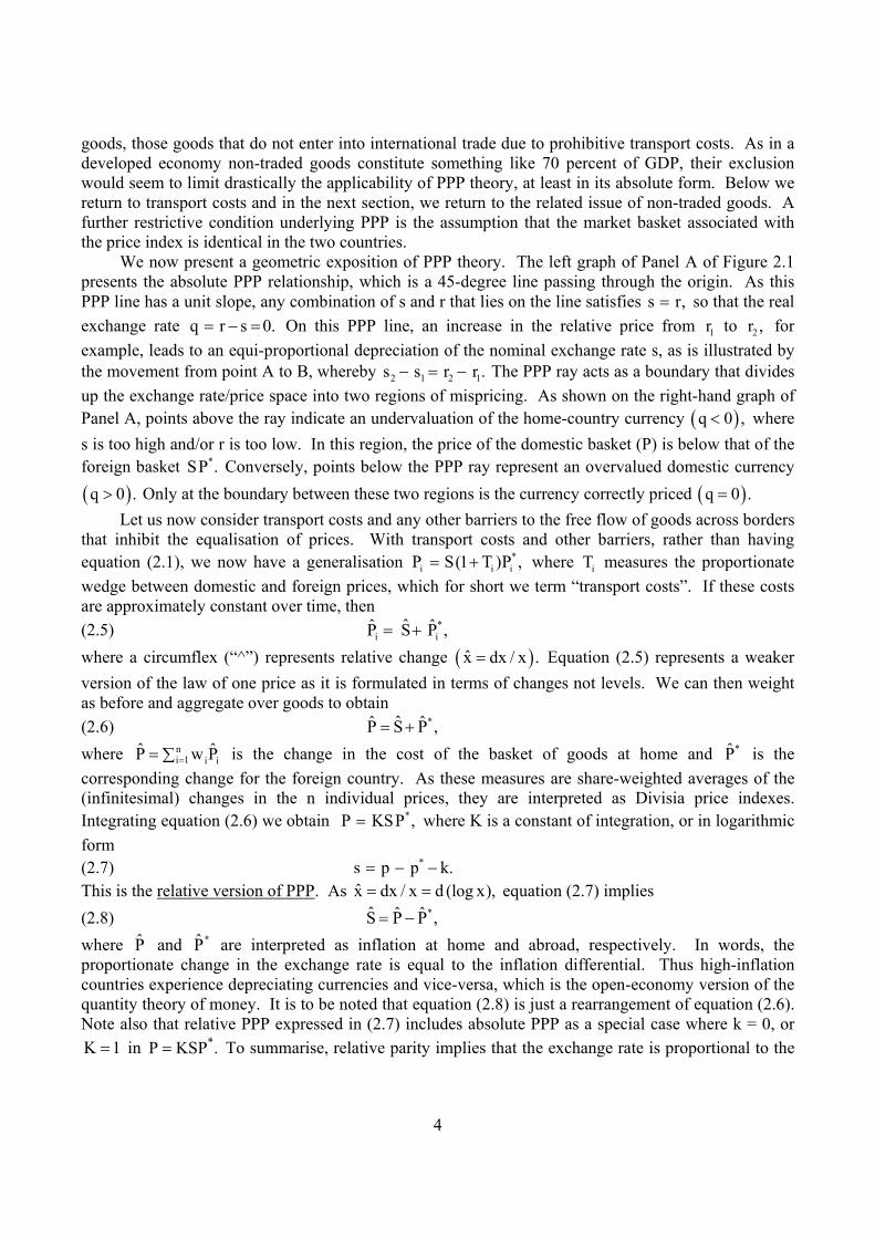
goods, those goods that do not enter into international trade due to prohibitive transport costs. As in a developed economy non-traded goods constitute something like 70 percent of GDP, their exclusion would seem to limit drastically the applicability of PPP theory, at least in its absolute form. Below we return to transport costs and in the next section, we return to the related issue of non-traded goods. A further restrictive condition underlying PPP is the assumption that the market basket associated with the price index is identical in the two countries.

We now present a geometric exposition of PPP theory. The left graph of Panel A of Figure 2.1 presents the absolute PPP relationship, which is a 45-degree line passing through the origin. As this PPP line has a unit slope, any combination of s and r that lies on the line satisfies s r,= so that the real exchange rate q r s 0.= − = On this PPP line, an increase in the relative price from 1r to 2r , for example, leads to an equi-proportional depreciation of the nominal exchange rate s, as is illustrated by the movement from point A to B, whereby 2 1 2 1s s r r .− = − The PPP ray acts as a boundary that divides up the exchange rate/price space into two regions of mispricing. As shown on the right-hand graph of Panel A, points above the ray indicate an undervaluation of the home-country currency ( )q 0 ,< where s is too high and/or r is too low. In this region, the price of the domestic basket (P) is below that of the foreign basket *SP . Conversely, points below the PPP ray represent an overvalued domestic currency

( )q 0 .> Only at the boundary between these two regions is the currency correctly priced ( )q 0 .= Let us now consider transport costs and any other barriers to the free flow of goods across borders

that inhibit the equalisation of prices. With transport costs and other barriers, rather than having equation (2.1), we now have a generalisation *

i i iP S(1 T )P ,= + where iT measures the proportionate wedge between domestic and foreign prices, which for short we term “transport costs”. If these costs are approximately constant over time, then (2.5) *

i iˆˆ ˆP S P ,= +

where a circumflex (“^”) represents relative change ( )x̂ dx / x .= Equation (2.5) represents a weaker version of the law of one price as it is formulated in terms of changes not levels. We can then weight as before and aggregate over goods to obtain (2.6) *ˆˆ ˆP S P ,= + where n

i 1 i iˆ ˆP w P== ∑ is the change in the cost of the basket of goods at home and *P̂ is the

corresponding change for the foreign country. As these measures are share-weighted averages of the (infinitesimal) changes in the n individual prices, they are interpreted as Divisia price indexes. Integrating equation (2.6) we obtain *P KSP ,= where K is a constant of integration, or in logarithmic form (2.7) *s p p k.= − − This is the relative version of PPP. As x̂ dx / x d (log x),= = equation (2.7) implies (2.8) *ˆ ˆ ˆS P P ,= − where P̂ and *P̂ are interpreted as inflation at home and abroad, respectively. In words, the proportionate change in the exchange rate is equal to the inflation differential. Thus high-inflation countries experience depreciating currencies and vice-versa, which is the open-economy version of the quantity theory of money. It is to be noted that equation (2.8) is just a rearrangement of equation (2.6). Note also that relative PPP expressed in (2.7) includes absolute PPP as a special case where k = 0, or K 1= in *P KSP .= To summarise, relative parity implies that the exchange rate is proportional to the

5

price ratio, with the factor of proportionality not necessarily equal to unity. Under absolute parity, the proportionality factor is unity so that the exchange rate equals the price ratio.3

Geometrically, under relative PPP the relationship between s and the relative price *ppr −= is a straight line of the form s r k,= − which is presented on the left graph of Panel B of Figure 2.1. Along this line, the real exchange rate is q r s k,= − = which is constant. This relative PPP line also has a unit slope, but an intercept k 0.− ≠ Again as we move up the line from A to B, an increase in the relative price still leads to an equiproportional depreciation in the nominal exchange rate, so that

2 1 2 1s s r r .− = − As before, points above the relative PPP line correspond to an undervaluation of the domestic currency ( )q k 0− < and those below the line correspond to an overvaluation ( )q k 0 ,− > but in comparison with absolute PPP, the boundary between the two regions is now “vertically displaced”, as indicated by the graph given on the right-hand side of Panel B in Figure 2.1.

Panel C for Figure 2.1 gives the case of stochastic PPP.4 If we denote the stochastic deviation from relative parity by e with 0)e(E = and variance 2 ,σ the real exchange rate is then the random variable ekq −= with 2var (q) 0,= σ > so that q is obviously not constant. Initially, suppose for simplicity that e is a discrete random variable and that 0e1 < and 0e2 > are its only possible values. When the shock is 1e 0,< we obtain a new, lower 45-degree line, 1s k e r,= − + + which has an intercept of 1k e ;− + similarly, 0e2 > results in the upper line on the left graph of Panel C. Consider the situation in which s is the exchange rate and r1 is the relative price, so that we are located at the point W on the left graph of Panel C. If there is now the same increase in the relative price as before, so that r rises from r1 to r2, then, in the presence of the shock e1, we move from W to the point X with the rate depreciating to s0. But if the shock is e2, the same relative price r2 leads to an exchange rate of s , as indicated by the point Y. More generally, if relative prices change within the range ]r,r[ 21 and if the shocks can now vary continuously within the range 1 2[ e , e ], then the exchange-rate/relative-price points lie somewhere in the shaded parallelogram WXYZ. Thus the relationship between the exchange rate and prices is s r k e,= − + which is the stochastic version of PPP. Due to the random shocks e, the exchange rate and prices are no longer proportionate. It is to be noted that the height of the shaded parallelogram exceeds its base, which accords with the idea that exchange rates are much more volatile than prices in the short run (Frenkel and Mussa, 1980). However in the long run, as

0)e(E = and thus E(s) r k,= − relative PPP holds and the expected value of the real exchange rate k)q(E = is constant. Here k is the long-run, or equilibrium value of the real exchange rate.

Therefore in the case of stochastic PPP, the real exchange rate q is not constant and fluctuates around k, so that exchange rates and prices are scattered around the 45-degree line. This is in contrast to relative PPP, in which q is a constant value for any combination of s and r and all (s, r) pairs locate exactly on the 45-degree line. In other words, stochastic PPP means that there exists a “neutral band” around the 45-degree line that contains values of the exchange rate and prices that identify the currency as being “correctly priced”. Under relative PPP, these points are interpreted as deviations from parity. Obviously, the width of the band is the key to this approach: if it is sufficiently wide, then all possible 3 A further issue about the distinction between absolute and relative PPP should be noted. Almost invariably statistical agencies publish information on the cost of a basket of goods in the form of a price index that has an arbitrary base, which determines the proportionality constant K. Such indexes can only be used for calculations of relative parity, not absolute. 4 For an earlier rendition of stochastic PPP, see Lan (2002). For related work, see MacDonald and Stein (1999). Note also that MacDonald (2007, p. 42) considers PPP within an environment in which there are transaction costs in moving goods from one country to another. According to this broader version of PPP, there exists a “neutral band” within which exchange rates and prices can fluctuate.

6

configurations of exchange rates and prices would be contained in the band, and the approach would be vacuous. On the other hand, if the band is sufficiently narrow, all observations would locate outside it, and the approach would always be rejected. One way to strike a balance between the “too wide” and “too narrow” band problems is to proceed probabilistically.

Consider the probability distribution of the real exchange rate q with k)q(E = and 2var(q) .=σ We commence with the symmetric case in which the probability of the exchange rate being undervalued ( )q k 0− < is 2α and the same 2α is the probability of the currency being overvalued

( )q k 0 ,− > where 0 1.< α < In other words, we can interpret 2α as the mass in each tail of the distribution, so that our task is to characterise the location of the tails. According to Chebyshev’s inequality

( )2

2Pr q k c ,cσ

− > ≤

where c is a positive constant. We interpret c as defining the boundary, so that 2 2/ c ,α = σ or 2c / .= σ α Thus the lower bound is 2k /− σ α and the upper bound is 2k / .+ σ α The region of

correct pricing is indicated in the area between the lines 'DD and 'FF on the right graph of Panel C, which is defined by (2.9) −k z q k z,≤ ≤ +

where z 2z / .= = σ α The points above the line DD ', which correspond to the case −< kq z, indicate that the currency is undervalued, while points below the line 'FF ( )q k z> + identify overvaluation. Statistically, if we have a number of observations on q, 100α× percent of these would lie outside the band and the remaining (1 ) 100−α × percent inside it. In the above situation, the deviations are symmetric around the mean, so that there are equal probabilities of currency undervaluation and overvaluation and z z.= In the more general case, the distribution of q is asymmetric and the long-run relative PPP line, EE ', does not lie mid-way between the two boundaries

'DD and FF '. The above analysis does not hinge on q following any particular probability distribution -- it is

distribution free. If we have information on the form of the distribution, then this additional information can be used to tighten the neutral band. Consider for the purpose of illustration the case of the normal distribution whereby 2q ~ N(k, )σ and 0.05.α = Under normality

q kPr 1.96 1.96 1 0.95,−⎡ ⎤− < < = −α =⎢ ⎥σ⎣ ⎦

so that the neutral band for q is [ ]k 1.96 , k 1.96 .− σ + σ Contrast the width of this band with that implied by the Chebyshev’s inequality, expression (2.9). With 0.05α = as before, we have z 2z / 20 4.47 ,= = σ α = σ = σ so that the neutral band is [ ]k 4.47 , k 4.47 .− σ + σ Thus the width of the band under normality is 2 1.96 ,× σ while under Chebyshev’s inequality, it is 2 4.47 ,× σ so that the additional information that the distribution is normal results in a shrinkage of the band by about 50 percent.

It is worth noting that this approach to currency valuation resembles hypothesis testing. To see this, imagine the existence of an unknown “true” state of the world in which the currency is either correctly or incorrectly priced, and we observe only whether or not the exchange-price configuration is located within the neutral band. There are four possible outcomes of the application of the approach:

7

(i) When the currency is in fact correctly priced and stochastic PPP identifies this situation accurately, i.e., the (s, r) point is located in the neutral band. As the inference is correct, the procedure works satisfactorily.

(ii) When the currency is in fact correctly priced, but stochastic PPP yields the conclusion that it is undervalued or overvalued. There is an 100α × percent probability of this incorrect inference being drawn, which is analogous to a Type I error.

(iii) When the currency is in fact incorrectly priced, but stochastic PPP indicates that the currency is correctly priced. This is similar to the case of a Type II error.

(iv) When the currency is in fact incorrectly priced, and stochastic PPP accurately indicates that the currency is incorrectly priced. In this situation, the correct inference is drawn.

The above taxonomy is summarised in the following table:

Does (s, r) lie in the neutral band? True currency pricing

Yes No

Correct Reliable inference Type I error

Incorrect Type II error Reliable inference

To conclude this section, consider an arbitrary combination of s and r, which is represented by the same point C in all three right-hand graphs of Figure 2.1. As C lies above the PPP ray in Panels A and B, both absolute and relative PPP indicate that the currency is undervalued. However, according to stochastic PPP (Panel C), the currency is correctly priced as the point C lies within the neutral band. This situation is likely to be frequently encountered in practice with many apparent departures from parity simply associated with the inherent volatility of currency markets. For example, some departures may be insufficient to justify the costs of moving goods internationally and/or taking a currency position, especially if they are expected to soon reverse themselves. Therefore, to value a currency, it is crucial that the proper distinction be made between the three versions of PPP.

3. The Workings of the Big Mac Index

The previous section highlighted the restrictive conditions under which absolute parity holds, viz., (i) the absence of barriers to international trade, which also implies the absence of nontraded goods; and (ii) identical baskets underlying the price indexes in the home and foreign countries. The weaker condition of relative PPP largely avoids the first problem, which accounts for its more frequent use in practice, but the problem of identical baskets remains. Surprisingly, the Big Mac Index (BMI) uses absolute parity in the context of a single-good basket, a Big Mac hamburger. In this section, we illustrate the workings of the BMI and as it purports to have much to say about the workings of the real-world currency markets, we assess how the Index deals with the above two restrictive conditions and how it performs in practice.

Though just a single good, a McDonald’s Big Mac hamburger has a variety of tradable ingredients such as ground beef, cheese, lettuce, onions, bread, etc., and non-tradable ingredients such as labour, rent, and electricity, as well as other ingredients such as cooking oil, pickles and sesame seeds. By estimating the Big Mac cost function using the prices of the various ingredients, Parsley and Wei (2007) recover the recipe in “broad” basket form. They find that the shares of important ingredients are:

Ingredient Cost share (%)

Tradable Beef 9.0 Cheese 9.4

8

Bread 12.1 30.5 Nontradable

Labour 45.6 Rent 4.6 Electricity 5.1 55.3

Other 14.2

Total 100.0

We can thus regard the price of a Big Mac as being the cost of a basket of inputs, just like P of the previous section is the cost of a market basket of goods. By comparing the price of a Big Mac in the US and other countries, The Economist magazine judges whether currencies are correctly priced based on the idea that a Big Mac should cost the same everywhere around the world when using a common currency. As the basket associated with the prices can be considered as being close to being identical in the home and foreign countries, the BMI cleverly avoids problem (ii) above associated with absolute PPP. But as transport costs and other trade barriers are not allowed when comparing prices, this is an application of absolute PPP. As discussed in the previous section, the arbitrage foundation of absolute parity applies to traded goods only. But non-traded goods prices can also be related across countries for at least two reasons. First, if there is substitution between traded and nontraded goods in production and consumption, then in a broad class of general equilibrium models, the change in the price of non-traded goods ( )NP̂ is a

weighted average of the changes in the prices of importables and exportables ( )X,Mˆ ˆP P :

( ) X1 ,= ω + −ωN Mˆ ˆ ˆP P P where 0 1≤ ω≤ . Thus if nontraded goods are good substitutes for importables,

the weight ω is large, so that the relative price N MP P is approximately constant, while a large value of 1−ω implies XNP P is approximately constant (see Sjaastad, 1980, for details). Provided the weight ω is approximately the same at home and abroad, if PPP equalises the prices of traded goods across countries, then there is at least a tendency for the same to be true for their weighted average, the price of non-traded goods. However, as this link is based on substitution in production and consumption, it could possibly take some time for these relative price changes to work themselves through the economy and for there to be full adjustment. Second, there is an expectations mechanism that may be quite rapid in its operation. If producers of non-traded goods know of the above link between their prices and those of traded goods, they may reasonably base their price expectations on it. This could then mean that in setting prices, these producers could employ as a short-cut the rule that they change their prices as soon as the exchange rate varies. An example is the plumber in Buenos Aires who puts up his prices as soon as the peso falls. These arguments provide a rationale for the inclusion of elements of the cost of non-traded goods in PPP calculations, such as the Big Mac Index.

Figure 3.1 reproduces the Big Mac article published in The Economist of 27th May 2006. As can be seen from column 3 of the table, the implied PPP of the dollar is just the ratio of the domestic Big Mac price in domestic currency (column 1) to that in the US in terms of dollars (first entry in column 1). This ratio is the purchasing power of one US dollar in terms of Big Macs. However, the actual exchange rate, presented in column 4, may not be the same as this PPP exchange rate. Column 5 is the percentage difference between the PPP exchange rate and the actual exchange rate, a positive (negative) value of which indicates over (under) -valuation of a currency. An overvalued currency indicates that domestic prices are higher than foreign prices [ *P /(SP ) 1> ], and vice-versa. Take as an

9

example Argentina, the second country from the top of the list in the table. The first and second entries in column 1 of the table within Figure 3.1 show that it costs US$3.10 to buy a Big Mac in the US, and 7.00 pesos in Argentina. Thus the implied PPP exchange rate is 7.00/3.10 = 2.26, as indicated by the second entry of column 3. As the actual exchange rate is 3.06, the Argentine peso is undervalued by ( )2 26 3 06 3 06 26. . .− = − percent (see the first entry in the last column of the table). Given the value of the peso and US prices, Argentine prices are too low, so that a movement towards parity would require some combination of a rise in Argentine prices and an appreciation of the peso.

Tables A1 and A2 contain the implied PPP exchange rates and nominal exchange rates of all countries that have their Big Mac data published at least once in The Economist since the inception of the Big Mac Index in 1986. Tables 3.1 and 3.2 are the companion tables for the 24 countries that have all data available over the period of 1994-2006; these data will be used in all computations that follow. In the previous paragraph, we showed that for Argentina in 2006 the BMI is as much as 26 percent below the market exchange rate. An element-by-element comparison of the first row of Table 3.1 with that of Table 3.2 reveals that there are similar large differences in most other years for this country. As will be discussed further below, the same problem of large deviations from parity occurs for most other countries. As under absolute parity these differences should be zero, this is not particularly encouraging for the proposition that BMI has economic content.

One other feature of Tables 3.1 and 3.2 is worthy of note. The last columns of these tables give the coefficients of variations of the implied PPPs and exchange rates in each country, and Figure 3.2 is the associated scatter. The points corresponding to Brazil, Poland and Russia are located far away from those for the other countries, due to the volatility of monetary conditions in these countries associated with currency redenominations. The left panel of Figure 3.2 shows that in 17 out of the remaining 21 countries, as the points lie above the 45-degree line, the implied PPPs are less volatile than the corresponding exchange rates. This difference between the behaviour of exchange rates and prices was noted long ago by Frenkel and Mussa (1980) who attributed it to the essential distinction between the nature of asset and goods markets. The exchange rate is the price of foreign money and as such, behaves like the prices of other assets traded in deep, organised markets such as shares, bonds and some commodities. The determination of asset prices tends to be dominated by expectations concerning the future course of events. As expectations change due to the receipt of new information, which is unpredictable, the net result is that changes in asset prices themselves are largely unpredictable, giving rise to the substantial volatility of these prices. By contrast, goods prices tend to be determined in flow markets in which expectations play a much less prominent role. It is for this reason that goods prices tend to be more tranquil over time, reflecting changes in the familiar microeconomic factors of incomes, supply conditions, etc. The Big Mac data reflect this difference between the volatility of asset and goods prices.

Under PPP, *P SP ,= or *P SP 1.= It is convenient to measure disparity logarithmically, so that for country c in year t, we define ( )*

ct ct ct tq log P S P ,= as in equation (2.4) where we referred to this

measure as the real exchange rate. This ctq , when multiplied by 100, is approximately the percentage difference between *

ct tP / P and ctS , the measure of disparity (or under- or over-valuation) used by The Economist (given in column 5 of the table in Figure 3.1). Under absolute PPP, ctq 0.= Table 3.3 and Figure 3.3 give ctq for each of the 24 countries over the 13-year period and as can be seen, there are frequent departures from absolute PPP. Additionally, in the majority of countries ctq fluctuates a lot around its mean over the 13-year period; the exceptions to this general rule are Britain, China, Hong Kong and Poland. One striking pattern is the one-sided nature of the disparities. Among the 24 countries under investigation, ten countries -- Australia, China, the Czech Republic, Hong Kong, Hungary, Malaysia, Poland, Russia, Singapore and Thailand -- always have undervalued currencies.

10

The currencies of Britain, Demark and Switzerland are always overvalued, while the Canadian dollar, the Mexican peso and the New Zealand dollar are undervalued in all but one year. Moreover, the Swedish krona is overvalued in all years except one. Thus for almost 10 3 3 1 17+ + + = cases out of a total of 24, the BMI declares the currencies to be continuously (or almost continuously) over- or under-valued for each of the 13 years. These strings of persistent disparities over a fairly lengthy period in two-thirds of the cases raise serious questions about the credibility of the BMI as a pricing rule for currencies. To assess the current value of a currency, it would seem desirable for a robust pricing rule to incorporate appropriately past mispricing. The sustained nature of the departures from PPP, departures that are distinctly one-sided, means that past mispricing is ignored by the BMI. Below, we explore further this problem.

To test the significance of the pattern of deviations from parity, we employ two tests, one based on a contingency table and the other a runs test. Consider again the signs of successive pricing errors. If these are independent, then the probability of the currency being over- or under-valued in year t 1+ is unaffected by mispricing in year t. To examine this hypothesis, in Table 3.4 we tabulate the mispricing for all currencies in all years, cross-classified by sign in consecutive years t and t 1.+ As the observed 2χ value is 183.8 (given in the last entry of the last column of the table), we reject the hypothesis of independence on a year-on-year basis. Next, we repeat this test with the horizon extended from 1 year to 2, 3, …, 12, and Table 3.5 reveals that independence is again rejected over most of these longer horizons whether or not overlapping observations are omitted.

Now consider a runs test. A run is a subsequence of consecutive numbers of the same sign, immediately preceded and followed by numbers of the opposite sign, or by the beginning or end of the sequence. If a currency is correctly priced, it is expected that the number of runs in the signs of the deviation is consistent with that of a random series. For example, the first row of Table 3.6 shows that for Argentina the signs of its q are + + + + − + − − − − − − − , which comprise four runs. If there are T observations and positive and negative values occur randomly, then the number of runs, R, is a random variable with mean ( ) ( )E R T 2T T T+ −= + and variance

( ) ( )2var R 2T T 2T T T T T 1 ,+ − + −= − − where T+ and T− are the total number of observations with positive and negative signs, respectively, with T T T.+ −+ = Asymptotically, the distribution of R is

normal and the test statistic ( )Z R E R var R ~ N(0,1).= −⎡ ⎤⎣ ⎦ The results, given in Table 3.6, show that the null of randomness is rejected for almost all of the 24 countries. Although this result is subject to the qualification that this test has only an asymptotic justification, the evidence against randomness seems to be reasonably compelling.

Next we test whether or not the disparities are significantly different from zero, which amounts to a test of bias in the BMI. The shaded regions of Figure 3.3 are the two-standard-error bands for the mean exchange rates. These bands include zero only for Argentina, Chile, Japan and South Korea, so we can reject the hypothesis that q 0= for the remaining 20 countries. In Figure 3.4 we present the mean real exchange rates with countries grouped into four regions. This figure reveals that all currencies except those for the five high-income European regions/countries -- the euro area, Britain, Sweden, Denmark and Switzerland -- are undervalued. It is notable that among the Asians, the currencies of China, Hong Kong, Malaysia and Thailand are all substantially undervalued.5 As exchange rates are expressed relative to the US dollar, some inferences about the value of the dollar can 5 The productivity-bias hypothesis of Balassa (1964) and Samuelson (1964) says that the currencies of rich (poor) countries are over (under) valued. While it is true that in Figure 3.4 the five countries (regions) with q 0> all have high incomes, countries with q 0< include Canada, Australia, New Zealand, Hong Kong and Singapore, all of which should probably also be classified as rich. Thus the evidence in Figure 3.4 does not provide unambiguous support for the productivity-bias hypothesis.

11

be drawn by averaging disparities over all non-dollar currencies, as is done in the third last row of Table 3.3. Thus we see that in 2006 on average the 24 currencies were undervalued by about 20 percent, which is equivalent to saying that the US dollar is overvalued by this amount. The value of the dollar over time is thus given by the entries of the third last row of Table 3.3 with the signs changed. Figure 3.5 plots these values of the dollar and as can be seen, it was most overvalued around 2001 and has been falling since then. The obvious qualification to this measure is that all 24 countries are equally weighted in valuing the dollar; more complex weighting schemes could be easily explored, but these would be unlikely to change the broad conclusion of an overvalued, but falling dollar.

Due to the 1997 Asian financial crisis, it is natural to divide the whole 13-year period into sub-periods, before and after 1997, as in Table 3.7. There are two notable features here. (i) In all but one country (Hong Kong, whose real exchange rate remains virtually unchanged), currencies become more undervalued (or less overvalued) following the Asian crisis. (ii) The changes in the means over the two periods are significant in 16 out of 24 countries. The results of testing the hypothesis that the real exchange rate is zero can be summarised as follows:

Period 1994-1997

(%) 1998-2006

(%) 1994-2006

(%) Significantly positive 38 17 21 Significantly negative 54 79 71 Insignificant 8 4 8 Total 100 100 100

Thus we see that sustained mispricing is almost the rule for the BMI. The BMI is meant to play the role of the long-term, or equilibrium exchange rate, to which the actual rate is attracted; in other words, an under- or overvaluation is meant to signal subsequent equilibrating adjustments of the exchange rate and/or prices. But lengthy periods of substantial, sustained and significant mispricing demonstrate that such a mechanism is not at work. In a fundamental sense the Big Mac Index fails, so that the Big Mac metric of currency mispricing cannot be taken at face value. In large part, the reason for this failure is that the BMI relies on absolute PPP, which ignores barriers to international trade. Fortunately, a simple modification to the BMI restores its predictive power, as is shown in the section after the next.

To summarise this section, we have established the following: • The BMI uses the cost of a Big Mac hamburger as the metric for judging whether or not the

currency is mispriced. As this product is made according to approximately the same recipe in all countries, the BMI avoids one of the major problems usually associated with absolute PPP. That problem is that the baskets underlying price indexes at home and abroad are likely to be substantially different, so that the ratio of the indexes reflects a combination of compositional disparities, as well as currency fundamentals.

• A well-known empirical regularity is that exchange rates are more volatile than prices. The Big Mac prices reflect this regularity.

• There are substantial, sustained and significant deviations of exchange rates from the BMI. The under- and over-valuations of currencies based on the BMI published by The Economist cannot be accepted as a reliable measure of mispricing. The BMI needs to be enhanced before it has substantial practical power.

4. The Bias-Adjusted BMI and the Speed of Adjustment

The above discussion implies that the BMI is a biased indicator of absolute currency values. Thus rather than absolute PPP holding in the form of *S P / P ,= we have ( )*S B P / P ,= where B is the

12

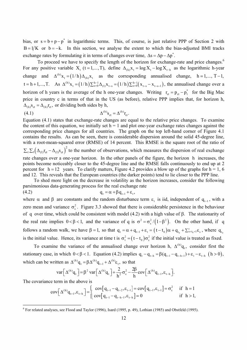
bias, or *s b p p= + − in logarithmic terms. This, of course, is just relative PPP of Section 2 with B 1 K= or b k.= − In this section, we analyse the extent to which the bias-adjusted BMI tracks exchange rates by formulating it in terms of changes over time, *s p p .Δ = Δ −Δ

To proceed we have to specify the length of the horizon for exchange-rate and price changes.6 For any positive variable tX (t 1,...,T),= define (h) t t t hx log X log X −Δ = − as the logarithmic h-year

change and ( )(h)t (h) tx 1/ h xΔ = Δ as the corresponding annualised change, h 1,..., T 1,= −

t h 1,...,T.= + As ( ) ( ) ( )(h) h 1 h 1s 0 s 0t (1) t s t s t s 1x 1/ h x 1/ h x x− −= =− − − −Δ = Δ = −∑ ∑ , the annualised change over a

horizon of h years is the average of the h one-year changes. Writing *ct ct tr p p= − for the Big Mac

price in country c in terms of that in the US (as before), relative PPP implies that, for horizon h, (h) ct (h) cts r ,Δ = Δ or dividing both sides by h,

(4.1) (h) (h)ct cts r .Δ = Δ

Equation (4.1) states that exchange-rate changes are equal to the relative price changes. To examine the content of this equation, we initially set h = 1 and plot one-year exchange rates changes against the corresponding price changes for all countries. The graph on the top left-hand corner of Figure 4.1 contains the results. As can be seen, there is considerable dispersion around the solid 45-degree line, with a root-mean-squared error (RMSE) of 14 percent. This RMSE is the square root of the ratio of

( )2c t (1) ct (1) ctr sΔ −Δ∑ ∑ to the number of observations, which measures the dispersion of real exchange

rate changes over a one-year horizon. In the other panels of the figure, the horizon h increases, the points become noticeably closer to the 45-degree line and the RMSE falls continuously to end up at 2 percent for h 12= years. To clarify matters, Figure 4.2 provides a blow up of the graphs for h = 1, 6 and 12. This reveals that the European countries (the darker points) tend to lie closer to the PPP line.

To shed more light on the decrease in volatility as the horizon increases, consider the following parsimonious data-generating process for the real exchange rate (4.2) t t 1 tq q ,−= α +β + ε where α and β are constants and the random disturbance term tε is iid, independent of t 1q − , with a zero mean and variance 2

εσ . Figure 3.3 showed that there is considerable persistence in the behaviour of q over time, which could be consistent with model (4.2) with a high value of .β The stationarity of the real rate implies 0 1,< β < and the variance of q is ( )2 2 2/ 1 .εσ = σ −β On the other hand, if q

follows a random walk, we have 1,β = so that t t 1 tq q −= α + + ε = ( ) 00

ts t 10 t st t q = +∑− α + + ε , where

0tq

is the initial value. Hence, its variance at time t is ( )2 2t 0t t εσ = − σ if the initial value is treated as fixed.

To examine the variance of the annualised change over horizon h, (h)tq ,Δ consider first the

stationary case, in which 0 1.< β < Equation (4.2) implies t t h t 1 t h 1 t t hq q (q q )− − − − −− = β − + ε − ε ( )h 0 ,>

which can be written as (h) (h) (h)t t 1 tq q ,−Δ = βΔ + Δ ε so that

(h) 2 (h) 2 (h)t t t 1 t h2

2 2var q var q cov q , .h hε − −

β⎡ ⎤ ⎡ ⎤ ⎡ ⎤Δ = β Δ + σ − Δ ε⎣ ⎦ ⎣ ⎦ ⎣ ⎦

The covariance term in the above is [ ] [ ][ ]

2t 1 t 2 t 1 t 1 t 1(h)

t 1 t ht 1 t h 1 t h

cov q q , cov q , if h 1cov q ,

cov q q , 0 if h 1,− − − − − ε

− −− − − −

⎧ − ε = ε = σ =⎪⎡ ⎤Δ ε = ⎨⎣ ⎦ − ε = >⎪⎩

6 For related analyses, see Flood and Taylor (1996), Isard (1995, p. 49), Lothian (1985) and Obstfeld (1995).

13

so that

(4.3)

2 22

(h)t

22 2

2(1 ) 2 if h 11 1

var q2 if h 1.

h (1 )

ε ε

ε

−β⎧ σ = σ =⎪ −β +β⎪⎡ ⎤Δ = ⎨⎣ ⎦⎪ σ >⎪ −β⎩

Therefore, we can see that (h)tvar q⎡ ⎤Δ⎣ ⎦ decreases when the horizon h increases for the stationary case.

This is represented in Panel A of Figure 4.3 by the point A and the reciprocal quadratic curve of the form (h) 2

tvar q 1/ h ,⎡ ⎤Δ ∝⎣ ⎦ with 0 6. .β =

If 1β = , equation (4.2) implies that ts t h 1t t h sq q h = − +−− = α + ε∑ . When divided by h, we have

(h) t1s t h 1t shq = − +Δ = α + ε∑ , so that

(4.4) 2t(h)

t s2s t h 1

1var q var ,h h

ε

= − +

σ⎡ ⎤⎡ ⎤Δ = ε =∑⎣ ⎦ ⎢ ⎥⎣ ⎦

which is represented in Panel A of Figure 4.3 by the reciprocal curve of the form (h)tvar q 1/ h⎡ ⎤Δ ∝⎣ ⎦ .

We can see that here (h)tvar q⎡ ⎤Δ⎣ ⎦ also declines, but at rate h, which is slower than the AR(1) case.

This contrast is more apparent by considering total volatility ( h )2 (h)

t tvar q h var q⎡ ⎤⎡ ⎤Δ = Δ⎣ ⎦ ⎣ ⎦ . From equations (4.3) for h 1> and (4.4), we have

(4.5) ( h )

22

t2

2 11var qh 1,

ε

ε

⎧ σ β <⎪⎡ ⎤ −βΔ = ⎨⎣ ⎦⎪ σ β =⎩

which is constant when 1β < and increases linearly when 1β = , as indicated in Panel B of Figure 4.3.

Equation (4.5) is a key result that shows that when the real rate is stationary, the total volatility is constant as the length of the horizon expands, while it increases in the non-stationary case. Although this is based on the simple AR(1) model, the implications carry over to more general cases. For a given horizon h, the RMSE of Figure 4.1 is the standard deviation of the annualised changes, or an estimate

of (h)tvar q⎡ ⎤Δ⎣ ⎦ . Thus h RMSE× is the standard deviation of the total changes, ( h ) tvar q⎡ ⎤Δ⎣ ⎦ , which

under stationarity will also be constant with respect to h. We use the RMSEs from Figure 4.1 in Figure 4.4 to plot h RMSE× against the horizon. As can be seen, total volatility first increases and after about 3 years fluctuates within a band that is less than 10 percentage points wide. It seems not unreasonable to interpret this evidence as saying real rates are stationary, that is, relative purchasing parity holds at longer horizons.

The above analysis shows that the speed of adjustment of exchange rates to prices is not rapid, which presumably reflects transaction costs, informational costs, sticky prices due to contracts and menu costs, etc. But over the medium-term of more than three years, the tendency for exchange rates to reflect PPP is clear. In the context of the discussion of Section 2, it seems that stochastic PPP with a relatively a high value of the variance 2σ is the way to think of the relationship between exchange rates and prices in the short term.

5. Does the BMI Predict Future Currency Movements?

In this section, we examine the predictive power of the Big Mac Index by asking the question, can a currency be expected to appreciate (depreciate) in the future if it is currently undervalued

14

(overvalued)? And if it does mean revert in this manner, how long does it take? For an early analysis along these lines, see Cumby (1996).

As our objective is to examine the information contained in the current BMI regarding future currency values, we start by defining the horizon for future changes in the real rate as (5.1) (h) t h t h tq q q ,+ +Δ = − which is the future change in q from the year t to t h.+ This total change in q over h years is just the sum of the corresponding h annual changes, ( )h 1 h 1

s 0 s 0(h) t h (1) t h s t h s t h s 1q q q q .− −= =+ + − + − + − −Δ = Δ = −∑ ∑

Regarding current mispricing, the use of tq would not be satisfactory due to the bias identified above. Instead we use (5.2) t td q q,= − with q the sample mean, which can be interpreted as the equilibrium exchange rate. Thus now the currency is over (under) valued if td 0 ( 0).> < Under PPP, deviations from parity die out, so that if

td 0 ( 0),> < the future value t hq + decreases (increases) relative to the current value tq . To examine whether this is the case, we plot in Figure 5.1 the subsequent changes (h) t hq +Δ against td using the 24-country Big Mac data for horizons of h 1,...,12= years. PPP predicts that the points lie in the second and fourth quadrants of the graphs, and Figure 5.1 shows this is indeed mostly the case with the pattern becoming more pronounced as the horizon increases. To examine the statistical significance of this pattern, we first carry out a 2χ -test of the independence of (h) t hq +Δ and td . 7 The test statistic is contained in the top box of each graph in Figure 5.1, and is significant for all horizons except 11 and 12 years (for which there are few observations), so we can reject independence. Figure 5.2 plots the test statistic against the horizon h and it can be seen that a maximum is reached for a horizon of h 5 or 6,= so that in this sense the current deviation best predicts subsequent changes over a five- or six-year horizon.

In each panel of Figure 5.1 we also report the least-squares estimates of the predictive regression (5.3) h h h

(h) t h t tq d u ,+Δ = η + φ +

where, for horizon h, hη is the intercept, hφ the slope and htu a zero-mean disturbance term. Panel A

of Table 5.1 reproduces the estimates of this regression in the first line for each horizon, while column 6 reproduces the 2χ values discussed in the previous paragraph; the information in column 7 will be discussed subsequently. To examine the effect of inclusion of an intercept, we report for each horizon the slope coefficient when the intercept is suppressed, and the results are qualitatively similar. Panel B of Table 5.1 redoes the analysis with non-overlapping observations only, and in all four sets of results -- overlapping and non-overlapping, with and without an intercept -- the slope coefficient is significantly negative, indicating that the adjustment goes in the expected direction.

To further interpret equation (5.3), we combine equations (5.1), (5.2) and (5.3) to obtain (5.4) ( ) ( )h h h h

t+h t tq = q + 1 q + u .η −φ φ +

Under PPP, t+hq converges to the equilibrium value q, so that (5.5) 0, 1h h .η = φ = − A test of restriction (5.5) reveals whether or not there is full adjustment to mispricing over horizon h. The F-statistics for (5.5) are presented in column 7 of Table 5.1 for the overlapping and non-overlapping cases. For the purposes of testing, the results for the non-overlapping case are more

7 This test is based on a 2 2× contingency table with rows the sign of td and columns the sign of t+h(h)Δ q .

15

reliable and as can be seen from Panel B, the F-statistic is minimised for a three-year horizon and is not significant. The F-statistic is also not significant for a five- and six-year horizons, but is significant for all other horizons. These results point to the conclusion that roughly speaking, over a period of three to six years there is more or less full adjustment of the rate to mispricing.

Figure 5.3 plots the estimated intercepts and slopes, h ,h andη φ against the horizon when overlapping observations are omitted. Three comments can be made. First, the intercepts are negative for most horizons, but many of the 95-percent confidence intervals include zero. Second, the slope generally decreases with h and the 95-percent confidence interval includes -1 for horizons 3 to 6 years. As the absolute value of hφ is the fraction of the total adjustment that occurs over horizon h, it is reasonable for a larger share of the adjustment to be completed over a longer horizon. Third, we should possibly pay more attention to the estimated slope, rather than the intercept. If, for some reason, the equilibrium rate differs from the mean q , then the difference would be absorbed into the intercept which becomes non-zero even if PPP holds.

Next, consider as an illustrative example the AR(1) case, equation (4.2), t t 1 tq q −= α +β + ε , so that

(5.6) h 1 hh h j

t h t t jj 1

(1 )q q .1

−−

+ +=

α −β= +β + β ε∑

−β

Equating the intercepts and slopes of the right-hand-sides of equations (5.4) and (5.6), we have ( ) ( ) ( )h h h 1q 1 1 ,−η − φ = α −β −β ( )h h1 ,φ + = β or

(5.7) h h 1q 1 ,⎛ ⎞η = β −⎜ ⎟β⎝ ⎠

h h 1.φ = β −

We use q 0.2,= − the grand average from the Big Mac data, and 0.6,β = as before, in equation (5.7) to plot the intercept hη and slope hφ against h, and Figure 5.4 gives the results. As these plots do not match those of Figure 5.3 too well, it seems that the actual data generation process is more complex than the simple AR(1) model.

Since the work of Meese and Rogoff (1983a,b), the random walk model has become the gold standard by which to judge the forecast performance of exchange-rate models. Accordingly, we compare the forecasts from the Big Mac Index and the bias-adjusted BMI with those from a random walk. Under the BMI, absolute parity holds and the forecast real exchange rate at any horizon h is zero, t hq 0;+ = the bias-adjusted BMI, as represented by equations (5.3) and (5.5), implies t hq q;+ = and the random walk predicts no change, t h tq q .+ = We compute the root-mean-squared error of the forecasts over all currencies and years for horizons h 1,...,12= , and Figure 5.5 shows that the random walk model outperform the BMI for all horizons, which is the familiar Meese-Rogoff result.8 However 8 Note that in addition to the RMSEs of Figure 5.5, earlier we presented another set in Figure 4.1. These are related as follows. For simplicity, suppose there are T realisations of one exchange rate, which we forecast for all horizons by sample mean q . Denote this for horizon h by

h 2Tt 11 t hRMSE (1/ T) (q q) ,= +

= −∑ which is a simplified expression for the RMSEs presented in Figure 5.5 associated with the bias-adjusted BMI. The corresponding simplified expression for the RMSEs of Figure 4.1 is

( ) ( ) ( )2h Tt 12 t h tRMSE 1 h 1/ T q q .= +

= −∑

If tq does not deviate too much from q, ( )h h2 1RMSE 1 h RMSE .≈ While this is only an approximation, this relationship

is likely to be the main reason that the RMSEs of Figure 4.1 decrease substantially with the horizon h, while those of Figure 5.5 do not exhibit this pattern.

16

the figure also reveals that beyond one-year horizons the bias-adjusted BMI beats the random walk. For example, for a 4-year horizon, the RMSE is about 40 percent for the BMI, 30 percent for the random walk and something less than 20 percent for the bias-adjusted BMI. This is an encouraging result for the bias-adjusted BMI.

This section can be summarised as follows: • The direction of future changes in currency values is clearly not independent of current

deviations from parity: Over-valued currencies subsequently depreciate, while under-valued ones appreciate.

• The adjustment to deviations from parity tends to be more or less fully complete over a period of three to six years.

• The bias-adjusted Big Max Index beats the random walk model for all but one-year horizons, demonstrating that it has considerable predictive power regarding future currency values.

6. The Split Between the Nominal Rate and Prices

In this section, we examine the relationship between mispricing and the two components of the real exchange rate -- the nominal exchange rate and inflation. We first examine empirically the behaviour of the two components over different horizons in the future, and then develop a simple geometric framework that highlights the relative flexibility of the exchange rate and prices.

From the definition of the real exchange rate, ( )t t t tq log P S P ,∗= and using the previous change

notation of ( )(h) t h t h tx log X X+ +Δ = we have the identity (6.1) (h) t h (h) t h (h) t hq s r ,+ + +Δ = −Δ + Δ

where, e. g., (h) t hr +Δ = (h) t h (h) t hp p∗+ +Δ − Δ is the cumulative inflation differential over h years in the

future. Equation (6.1) decomposes the future change in the real rate into the corresponding changes in the nominal rate and the inflation differential. A positive value of (h) t hq +Δ means that the inflation differential exceeds the nominal depreciation of the exchange rate, which amounts to a real appreciation over an h-year horizon.

To examine the mean-reverting behaviour of the two components over different horizons, consider predictive regressions analogous to equation (5.3): (6.2) h h h

(h) t+h s s t st-Δ s d u ,= η + φ + h h h(h) t+h r r t rtΔ r d u ,= η + φ +

In the AR(1) case, j

j 0t t 1 t t jq q q ∞=− −

∑= α + β + ε = + β ε , and the simplified expression for the first version of the of the square of the RMSE is

( ) ( ) ( )h

1

2T2 j

t h jt 1 j 0

RMSE AR(1)| 1 T∞

+ −= =

= ∑ ∑ β ε , with ( )h

1

2

2

2

RMSE AR(1)1

E | .ε=− β

σ⎡ ⎤⎣ ⎦

The corresponding second version is

( ) ( )( ) ( )h

2

2T2 2 j

t h j t jt 1 j 0

RMSE AR(1)| 1 h 1 T∞

+ − −= =

= ∑ ∑ β ε − ε⎡ ⎤⎢ ⎥⎣ ⎦

, with ( ) ( )h

2 2

2

2

h 22 21

RMSE AR(1) .1

Eh

| ε− β

− β

σ=⎡ ⎤

⎣ ⎦

As ( ) ( ) ( )h h

2 1

2 2h 2RMSE AR(1) RMSE AR(1)E E| 2 1 2 h | ,= − β⎡ ⎤ ⎡ ⎤⎡ ⎤⎣ ⎦⎣ ⎦ ⎣ ⎦i there is a similar relationship between the two

measures whereby the first is independent of the horizon, while the second declines with h.

17

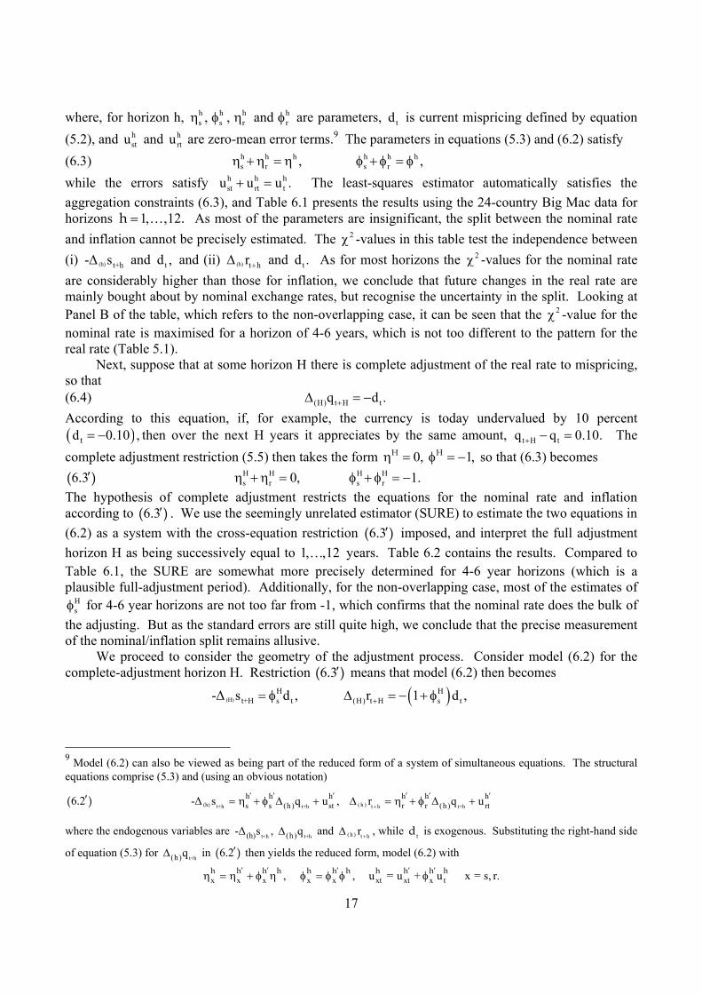
where, for horizon h, h hs s, ,η φ h

rη and hrφ are parameters, td is current mispricing defined by equation

(5.2), and hstu and h

rtu are zero-mean error terms.9 The parameters in equations (5.3) and (6.2) satisfy (6.3) h h h

s r ,η +η = η h h hs r ,φ + φ = φ

while the errors satisfy h h hst rt tu u u .+ = The least-squares estimator automatically satisfies the

aggregation constraints (6.3), and Table 6.1 presents the results using the 24-country Big Mac data for horizons 1, ,12= …h . As most of the parameters are insignificant, the split between the nominal rate and inflation cannot be precisely estimated. The 2χ -values in this table test the independence between (i) (h) t+h-Δ s and td , and (ii) (h) t hr +Δ and td . As for most horizons the 2χ -values for the nominal rate are considerably higher than those for inflation, we conclude that future changes in the real rate are mainly bought about by nominal exchange rates, but recognise the uncertainty in the split. Looking at Panel B of the table, which refers to the non-overlapping case, it can be seen that the 2χ -value for the nominal rate is maximised for a horizon of 4-6 years, which is not too different to the pattern for the real rate (Table 5.1).

Next, suppose that at some horizon H there is complete adjustment of the real rate to mispricing, so that (6.4) (H) t H tq d .+Δ = − According to this equation, if, for example, the currency is today undervalued by 10 percent ( )d 0 10 ,t .= − then over the next H years it appreciates by the same amount, t H tq q 0.10.+ − = The complete adjustment restriction (5.5) then takes the form 0, 1,H Hη = φ = − so that (6.3) becomes 6 3( . )′ H H

s r 0,η +η = H Hs r 1.φ + φ = −

The hypothesis of complete adjustment restricts the equations for the nominal rate and inflation according to 6 3( . )′ . We use the seemingly unrelated estimator (SURE) to estimate the two equations in (6.2) as a system with the cross-equation restriction 6 3( . )′ imposed, and interpret the full adjustment horizon H as being successively equal to 1,…,12 years. Table 6.2 contains the results. Compared to Table 6.1, the SURE are somewhat more precisely determined for 4-6 year horizons (which is a plausible full-adjustment period). Additionally, for the non-overlapping case, most of the estimates of

Hsφ for 4-6 year horizons are not too far from -1, which confirms that the nominal rate does the bulk of

the adjusting. But as the standard errors are still quite high, we conclude that the precise measurement of the nominal/inflation split remains allusive.

We proceed to consider the geometry of the adjustment process. Consider model (6.2) for the complete-adjustment horizon H. Restriction 6 3( . )′ means that model (6.2) then becomes

(H)H

t+H s t-Δ s d ,= φ ( )H(H) t H s tr 1 d ,+Δ = − + φ

9 Model (6.2) can also be viewed as being part of the reduced form of a system of simultaneous equations. The structural equations comprise (5.3) and (using an obvious notation)

6 2( . )′ t+h t+h(h)h h hs s (h) st-Δ s q u ,′ ′ ′= η + φ Δ + t h t+h( h )

h h hr r (h) rtr q u

+

′ ′ ′Δ = η + φ Δ +

where the endogenous variables are t+h t+h(h) (h)-Δ s , qΔ and t h( h ) r +Δ , while td is exogenous. Substituting the right-hand side

of equation (5.3) for t+h(h)qΔ in 6 2( . )′ then yields the reduced form, model (6.2) with

x x x x x xt xt x t, , u = u + u x = s, r.h h h h h h h h h h h′ ′ ′ ′ ′η = η + φ η φ = φ φ φ

18

where for simplicity we have suppressed the intercepts and set the disturbances at their expected values of zero. The above equations can be written as (6.5) ( )(H) t H t (H) t H ts d , r 1 d ,+ +Δ = γ Δ = − − γ

where Hsγ = −φ . If the currency is undervalued ( )td 0 ,< then prices at home are too low relative to

those abroad, that is, t t tp s p q.∗< + + Thus we expect td 0< to be associated with (i) a future nominal appreciation, (H) t Hs 0,+Δ ≤ implying that 0,γ ≥ and/or (ii) a rise in relative inflation, (H) t Hr 0,+Δ ≥

implying ( )1 0.− − γ ≤ Accordingly, 0 1,≤ γ ≤ which means that the nominal rate changes by a fraction γ of the mispricing, while relative inflation changes by the remainder 1− γ . When the nominal rate does most of the adjusting, the parameter 0 5.γ > , and we have the ranking of changes

(H) t H (H) t H tr s d .+ +Δ < Δ < In words, the change in the rate is bracketed by the change in relative inflation and the initial mispricing.

Combining the two equations in (6.5) to eliminate td yields

(6.6) (H) t H (H) t Hs r .1+ +

⎛ ⎞γΔ = − Δ⎜ ⎟− γ⎝ ⎠

As the parameter γ is a positive fraction, the ratio ( )1−γ − γ on the right-hand side of the above falls in the range [ ]- ,0 .∞ Equation (6.6) describes the simultaneous adjustment of the exchange rate and prices in the future to current mispricing, with ( )1−γ − γ the elasticity of the rate with respect to the

price ratio *P P along the adjustment path. It is to be noted that as equation (6.6) deals with the equilibrating adjustments to mispricing, or a deviation from parity, this equation does not describe a PPP-type of relation whereby the rate and prices move proportionally. It follows from the way in which the deviation from equilibrium is defined, t td q q,= − together with the definition of the real exchange rate, *q p p s,= − − that a deviation of either sign results in equilibrating adjustments in the nominal rate and inflation that are negatively correlated. This is the reason why the elasticity in equation (6.6), ( )1−γ − γ , is negative. This elasticity characterises the trade-off between a higher nominal rate and a lower price level, and vice-versa, required to return the real rate back to its equilibrium value q.

The schedule FF in Figure 6.1 corresponds to equation (6.6). This schedule passes through the origin and has slope ( )1 0− γ − γ < that reflects the nature of the flexibility of the monetary side of the economy, that is, the relative flexibility of the rate as compared to prices. Going back to equation (6.5), when the nominal rate bears all of adjustment to mispricing, and relative inflation remains unchanged,

1γ = and 1 0,− γ = and the FF schedule is vertical. In the opposite extreme where the rate is fixed, 0,γ = 1 1− γ = and FF coincides with the horizontal axis. In a fundamental sense, the slope of FF

reflects the relative cost of changes in the exchange rate, as compared to price changes. Related considerations include whether or not the country pursues inflation targeting as the objective of monetary policy, and the extent to which the value of the currency is “managed” by the monetary authorities.

One way to obtain some additional information regarding the split between the nominal rate and inflation is to employ the signal extraction technique (Lucas, 1973). Write the real exchange rate as the sum of its two components as (6.7) q r x= + ,

19

where *r p p= − is the relative price and x s q r= − = − is the negative nominal rate, the logarithmic foreign currency cost of a unit of domestic currency.10 Assume that (i) r is normally distributed with mean r and variance 2

rσ ; (ii) x is normal with mean x and variance 2xσ ; and (iii) r and x are

orthogonal. Our objective is to forecast x given q. We start with a linear conditional forecast of r, (6.8) fr q= θ+ κ , where the subscript “f” denotes the forecast. Minimisation of the mean squared error, defined as

2fE(r r)− , gives

(6.9) (1 ) r xθ = − κ − κ , 2r

2 2x r

.σκ =

σ +σ

Substituting the first member of (6.9) into (6.8) yields fr (1 ) r (q x)= − κ + κ − . Based on equation (6.7), we then have (6.10) f f fE(x | r ) q r (1 )(q r ) x= − = − κ − + κ . The above equation shows that the conditional forecast of the nominal rate is a weighted average of (i) the deviation of the real rate from the long-run relative price and (ii) the historical mean of the nominal rate. If 2 2 2

x s rσ = σ σ (as seems to be the case empirically), the second member of (6.9) gives 0κ ≈ , so that the real rate term in (6.10) is accorded most of the weight in forecasting the nominal rate. That is, expression (6.10) becomes f fE(x | r ) q r≈ − , which implies f fE( x | r ) qΔ ≈ Δ . In words, the future change in the real rate is almost entirely brought about by the nominal rate adjusting. In the context of the full-adjustment horizon H, we can then write equation (6.4) as (H) t H ts d+Δ ≈ , which from equation (6.5), means 1γ ≈ and the FF schedule in Figure 6.1 is near vertical in this case.

To be able to say where the economy locates on FF, we need more information regarding the link between mispricing, the change in the exchange rate and inflation. This is provided by combining equation (6.4) and identity of (6.1) for h H := (6.11) (H) t H t (H) t Hs d r .+ +Δ = + Δ To interpret this equation, first consider the overvaluation case, so that td 0.> Equation (6.11) then gives the combinations of the future nominal depreciation and higher inflation at home required to eliminate the overvaluation. These combinations are represented by the schedule OO (for overvaluation) in Figure 6.1. This schedule has a slope of 45-degrees and an intercept on the vertical axis of td 0.> As the schedule indicates, the initial overvaluation could lead to (i) an equiproportional

nominal depreciation with inflation unchanged ( )(H) t H t (H) t Hs d , r 0 ;+ +Δ = Δ = (ii) no change in the

nominal rate, with all of the adjustment falling on inflation ( )(H) t H (H) t H ts 0, r d ;+ +Δ = Δ = − or (iii) any combination thereof. The overall equilibrium is given by the point E in Figure 6.1, the intersection of the OO and FF schedules. As can be seen, the overvaluation leads to a sharing of the adjustment between a depreciation and a slowing of inflation. It is to be noted that the point E is uniquely determined by (i) the initial overvaluation, which gives the location of OO; and (ii) the degree of relative flexibility of the exchange rate, as measured by the slope of FF.11

10 In this paragraph, for notational simplicity we suppress subscript t for q, r and x (or s). 11 The intercepts in the two equations in (6.2), ,h h

s randη η represent the changes in the rate and relative inflation that occur for reasons other than mispricing. For simplicity of exposition, in the above we set the intercepts to zero. When these terms are nonzero, equation (6.6) becomes

20

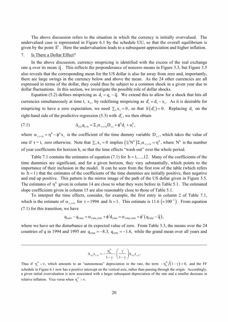
The above discussion refers to the situation in which the currency is initially overvalued. The undervalued case is represented in Figure 6.1 by the schedule UU, so that the overall equilibrium is given by the point E′ . Here the undervaluation leads to a subsequent appreciation and higher inflation.

7. Is There a Dollar Effect?

In the above discussion, currency mispricing is identified with the excess of the real exchange rate q over its mean q . This reflects the preponderance of nonzero means in Figure 3.3, but Figure 3.5 also reveals that the corresponding mean for the US dollar is also far away from zero and, importantly, there are large swings in the currency below and above the mean. As the 24 other currencies are all expressed in terms of the dollar, they could thus be subject to a common shock in a given year due to dollar fluctuations. In this section, we investigate the possible role of dollar shocks.

Equation (5.2) defines mispricing as t td q q.= − We extend this to allow for a shock that hits all currencies simultaneously at time t, tx , by redefining mispricing as t t td d x .′ = − As it is desirable for mispricing to have a zero expectation, we need tx 0t∑ = , so that ( )tE d 0.′ = Replacing td on the right-hand side of the predictive regression (5.3) with td′ , we then obtain

(7.1) h h(h) t h , h ,t t tq D d u ,+ τ τ τ+ τΔ = Σ α + φ +

where h h, h xτ τ+ τα = η −φ is the coefficient of the time dummy variable ,tDτ , which takes the value of

one if τ = t, zero otherwise. Note that tx 0t∑ = implies ( )h h, h1 N τ τ τ+Σ α = η , where hN is the number

of year coefficients for horizon h, so that the time effects “wash out” over the whole period.

Table 7.1 contains the estimates of equation (7.1) for 1, ,12.h = … Many of the coefficients of the time dummies are significant, and for a given horizon, they vary substantially, which points to the importance of their inclusion in the model. It can be seen from the first row of the table (which refers to 1h = ) that the estimates of the coefficients of the time dummies are initially positive, then negative and end up positive. This pattern is the mirror image of the path of the US dollar given in Figure 3.5. The estimates of hη given in column 14 are close to what they were before in Table 5.1. The estimated slope coefficients given in column 15 are also reasonably close to those of Table 5.1.

To interpret the time effects, consider, for example, the first entry in column 2 of Table 7.1, which is the estimate of , hτ τ+α for 1994τ = and 1h = . This estimate is 11.6 ( )1100−× . From equation (7.1) for this transition, we have

( )1 11995 1994 1994,1995 1994 1994,1995 1994q q d q q ,− = α + φ = α + φ −

where we have set the disturbance at its expected value of zero. From Table 3.3, the means over the 24 countries of q in 1994 and 1995 are 1994 1995q 8.3, q 1.6,= − = − while the grand mean over all years and

H

( H ) t H ( H ) t Hss r

1 1.

+ +

η γΔ = − − Δ

− γ − γ

⎛ ⎞⎜ ⎟⎝ ⎠

Thus if 0H

s <η , which amounts to an “autonomous” depreciation in the rate, the term ( )Hs 1 0,−η − γ > and the FF

schedule in Figure 6.1 now has a positive intercept on the vertical axis, rather than passing through the origin. Accordingly, a given initial overvaluation is now associated with a larger subsequent depreciation of the rate and a smaller decrease in relative inflation. Vice versa when 0

H

s >η .

21

currencies is ( )119 9 100q . all .−= − × Using these values, together with the estimate from Table 7.1 of 1φ of -0.4 (first entry of column 15), we have

(7.2) ( ) ( ) ( )1 11994,1995 1995 1994 1994q q q q 1.6 8.3 0.4 8.3 19.9 11.3 all 100 ,−α = − −φ − = − + + − + = ×

which is sufficiently close to the estimated intercept of 11.6 percent. Accordingly, the coefficient of the time dummy measures the cross-currency average of the change in q over the relevant horizon, after adjusting for the initial mispricing as measured by the term h

tdφ . Note that if 1 1,φ = − as it is under the hypothesis of full adjustment, then equation (7.2) simplifies to 1994,1995 1995q q,α = − which is just the deviation of q in the relevant year from the grand mean. As the estimated slope coefficient for 3h = in Panel A of Table 7.1 is very close to -1, we consider this case to illustrate this point. Column 2 of the table below contains the estimated coefficients of the time dummies, from the third row of Panel A of Table 7.1, corresponding to 3h = ; column 3 below contains the cross-currency means from Table 3.3; and column 4 contains the deviations from the grand mean of -19.86:

Year t+3 Estimated time effect

Cross-currency

mean

Deviation of cross-currency

mean from grand mean

(1) (2) (3) (4)

1997 9.73 -10.11 9.75 1998 -5.12 -24.94 -5.08 1999 -1.78 -21.61 -1.75 2000 -7.07 -26.90 -7.04 2001 -11.93 -31.80 -11.94 2002 -10.95 -30.81 -10.95 2003 -7.57 -27.44 -7.58 2004 -7.10 -26.98 -7.12 2005 -4.49 -24.37 -4.51 2006 0.79 -19.08 0.78

Note: All entries are to be divided by 100.

The close agreement of columns 2 and 4 confirms the interpretation of the time effects as the deviations from the grand mean under the condition 1hφ = − . This is why the time effects mirror the path of the dollar, mentioned in the paragraph above.

Next, we add time effects to the analysis of the split between the nominal rate and prices. In broad outline, this extension reveals little change from the results of Section 6 where the time effects are omitted. The detailed results are contained in Tables A4-A6 of the Appendix. In particular, we continue to find that it is difficult to quantity the split in a precise manner.

To summarise, the persistent swings of the dollar play a role in the adjustment to mispricing of non-dollar currencies. But even when these effects are allowed for, in broad outline the results of Sections 5 and 6 continue to hold: Within a period of three to six years, currency mispricing is more or less eliminated; but the split between changes in the nominal rate and relative prices in the adjustment process cannot be precisely estimated.

8. The Burgernomics Literature

22

This section reviews the literature on the Big Mac Index. Cumby (1996) is widely known as the first Burgernomics paper and was originally a 1995 Georgetown University working paper. Almost at the same time however, Ong (1995) was presented at the ANU/UWA PhD Conference in Economics and Business in Perth and later published as Ong (1997). As far as we are aware, there are in total eighteen academic papers and one book on the Big Mac Index/Burgernomics. Table 9.1 lists these publications in chronicle order. These papers can be broadly grouped into two categories, (i) the basic foundations and (ii) “adventurous” applications.

Regarding basic foundations, Cumby (1996) finds out that half-life of deviations from the Big Mac parity is about one year, and these deviations provide significant information for forecasting exchange rates and Big Mac prices. Lutz (2001) applies Cumby’s methodology to 12 price series published by the bank UBS as well as aggregate CPI data. Click (1996), Fujiki and Kitamura (2003) and Caetano et al. (2004) find country incomes to be important in explaining deviations from Big Mac PPP. Yang (2004) uses the BMI to evaluate the Chinese yuan and finds that currencies of low-income countries are overvalued due to the insufficient weight accorded to nontradables. Ong (1997) finds that Big Macs are surprisingly accurate in tracking exchange rates over the long run. She also proposes the “No-Frills Index” by excluding nontradable components from the Big Mac Index, and establishes that this performs better than the BMI. Using Big Mac prices, Ong (1998a) analyses the Asian currency crisis, while Ong (1998b), Ong and Mitchell (2000), and Ashenfelter and Jurajda (2001) compare wages in different countries. Ong (2003) is the only book on Burgernomics, and this comprises a series of papers by her and coauthors. Chen et al. (2005) compare the behaviour of Big Mac prices with CPIs and find that the BMI supports the validity of PPP better than the CPI does. Pakko and Pollard (1996, 2003) conclude that Big Macs are a useful but flawed PPP measure as deviations from absolute PPP are persistent while those from relative PPP are transitory. Parsley and Wei (2007) relate the price of a Big Mac to the costs of its ingredients and find that the speed of convergence of the overall Big Mac real exchange rate is bracketed by that for its tradable and nontradable inputs.

Annaert and Ceuster (1997) pursue of different line of research in one of the first adventurous applications of Burgernomics. They construct currency portfolios selected on the basis of the Big Mac Index whereby undervalued currencies are bought and undervalued ones sold, and their results show that Big Macs can serve as a useful international asset allocator. Given their volatility, exchange rates are notoriously difficult to forecast. As the previous US Fed Chairman, Alan Greenspan (2004), puts it, “despite extensive efforts on the part of analysts, to my knowledge, no model projecting directional movements in exchange rates is significantly superior to tossing a coin.” There is now an emerging stream of Burgernomics that investigates whether the BMI can be used to forecast exchange rates. Lan (2006) uses Big Mac prices to forecast the whole distribution of future exchange rates, employing a novel iterative approach to adjust for econometric problems associated with the estimation of dynamic panel models where the number of observations is not large. The provision of the whole distribution emphasises forecast uncertainty that enables users to make financial decisions in an informed manner with the appropriate degree of caution. Clements and Lan (2006) extend Lan (2006) and use Monte Carlo simulations to provide real-time exchange-rate forecasts for any horizon into the future.

9. Concluding Comments

The Economist magazine advocates as a currency pricing rule the formula *S = P P , where S is the exchange rate (the domestic currency cost of one US dollar), P is the price of a Big Mac hamburger in the country in question and P∗ is the price in the US. Thus an increase in the domestic price, relative to the US price, leads to a depreciation of the domestic currency. The rule is a precise, numerical relationship between the exchange rate and the relative price that can be used to identify mispricing of the currency in a quick and convenient way. This is a novel and controversial application

23

of the purchasing power parity theory of exchange rates that is known as the Big Mac Index and is published annually by The Economist for a large number of currencies.

The cost of a full-page advertisement in The Economist must be something like $US50,000. For the magazine to continue to publish an article on the Big Mac Index each year for 21 years means that it is worth this opportunity cost, at least in the mind of the editor. This paper assessed the broader value of the BMI by analysing its properties and ability to track exchange rates. The major findings of the paper are:

• The index is a biased predictor of currency values. • Once the bias is allowed for, the index tracks exchange rates reasonably well over the

medium to longer term in accordance with relative purchasing power parity theory. • The index is at least as good as the industry standard, the random walk model, in predicting

future currency values for all but short-term horizons. • Future nominal exchange rates are more responsive than prices to currency mispricing, but

this split is difficult to determine precisely. Thus, while it is not perfect, as the cost of the magazine is less than $US10, the index seems to provide good value for money. In showing that relative prices act as an “attractor” or “anchor” for exchange rates over the longer term, our results also have implications for exchange-rate economics: As currencies of high (low)-inflation countries depreciate (appreciate), over longer horizons economic fundamentals tend to dominate currency pricing.

24

APPENDIX

The Big Mac Data

The Economist magazine has been publishing the Big Mac index on an annual basis since 1986. The data presented in Tables A1, A2 and A3 are compiled from a number of issues of the magazine from 1986 to 2006. They consist of, respectively, the implied PPP exchange rates, nominal exchange rates and real exchange rates of all countries that have appeared at least once in The Economist during the 21-year period.

We have made adjustments for three discrepancies found in the published data. First, Chile’s 1999 Big Mac price and its corresponding implied PPP exchange rate are given as Peso 1,25 and 518, respectively, in The Economist. As the prices for this country in other years are about 1,250 pesos, we suspect the price should be 1,250 (rather than 1,25). Then we recompute the implied PPP exchange rate as 514.4 and use that in our table (rather than the published value 518). Second, the implied PPP exchange rate for Brazil in 1986 is given as 7.8 in The Economist. As this is inconsistent with our own calculation using the published Big Mac prices, the implied PPP exchange rate of 1.562 is used instead. Finally, the published PPP exchange rate for Denmark in 1998 is 9.28, while we have computed the rate at 9.297 using the published Big Mac prices; here again we use our internally-consistent figure.

In the text of the paper, we use the Big Mac data for 24 countries/areas over the period of 1994 to 2006, so that the total number of observations is 24 13 312.× = Tables 3.1-3.3 show the respective implied PPP exchange rates, nominal exchange rates and real exchange rates. In four instances, Big Mac prices and nominal exchange rates are missing: New Zealand (1994), China (1996), Hungary (1996), and the Czech Republic (1999). For these cases, nominal exchange rates are taken from the International Financial Statistics database published by the International Monetary Fund. The Big Mac prices are computed on the basis of the one-year percentage change in the Consumer Price Index (hereafter CPI), also taken from the IFS database. For example, we compute the price of a Big Mac hamburger in China in April 1996 as follows:

c,1997c,1996

c,1997

P 9.7P 9.39936,1 1 3.19847 /100

= = =+ π +

where c,1997π is the percentage change in the CPI from 1996 to 1997 in China. As the euro was not introduced until 1999, official data are unavailable for this currency from

1994 to 1998. However, the Big Mac data for the six member countries included in our data -- Belgium, France, Germany, Italy, Holland, and Spain -- exist for the pre-euro period. To calculate the implied PPP exchange rate of the euro during this period, we first convert the prices of the Big Mac hamburger to euros for these six countries using the exchange rates given on the InforEuro website.12 We define “the” euro price of a Big Mac as the unweighted average of the euro prices for these six countries. We then divide it by the US price of a Big Mac hamburger in US dollars to obtain the implied PPP exchange rate for Euroland. We obtain the corresponding “€/$” nominal exchange rates as follows. First, we calculate the “€/$” exchange rate for each member country by dividing the “DC/$” rate by the “DC/€” rate, where DC denotes the domestic currency so that, for example, DC/$ is the domestic currency cost of one US dollar. Second, as these “€/$” rates are not necessarily the same in the six countries, we take the unweighted average. The required nominal exchange rates are from both The Economist and the InforEuro website.

Additional Results with Time Effects

12 http://europa.eu.int/comm/budget/inforeuro/index.cfm?fuseaction=dsp_html_monthly_rates&Language=en.

25

Tables 6.1 and 6.2 of the text give the results for the predictive regressions when the real rate is decomposed into the nominal rate and relative inflation components. Tables A4-A6 of this appendix give the corresponding results when time effects are added.

26

REFERENCES Annaert, J., and M. J. K. Ceuster (1997). “The Big Mac: More than a Junk Asset Allocator?”

International Review of Financial Analysis 6: 79-192. Ashenfelter, O., and S. Jurajda (2001). “Cross-country Comparison of Wage Rates: The Big Mac

Index.” Unpublished paper, available at http://economics.uchicago.edu/download/bigmac.pdf. Balassa, B. (1964). “The Purchasing Power Parity Doctrine: A Reappraisal.” Journal of Political

Economy 72: 584-96. Caetano, S., G. Moura and S. Da Silva (2004). “Big Mac Parity, Income and Trade.” Economics

Bulletin 6: 1-8. Chen, C.-F., C.-H. Shen and C.-A. Wang (2005). “Does PPP hold for Big Mac Prices or the Consumer

Price Index? Evidence from Panel Cointegration.” Unpublished manuscript, National Dong Hwa University, Taiwan.

Clements, K. W., and Y. Lan (2006). “A New Approach to Forecasting Exchange Rates.” Discussion Paper No. 06.29, Economics Program, The University of Western Australia.

Paper presented to the 19th Australasian Finance and Banking Conference, 13-15 December, Sydney, Australia.

Click, R. W. (1996). “Contrarian MacParity.” Economics Letters 53: 209-12. Cumby, R. E. (1996). "Forecasting Exchange Rates and Relative Prices with the Hamburger Standard:

Is What You Want What You Get with McParity?" NBER Working Paper 5675. Flood, R., and M. Taylor (1996). “Exchange Rate Economics: What’s Wrong with the Conventional

Macro Approach?” In J. Frankel, G. Galli and A. Giocannini (eds) The Microstructure of Foreign Exchange Markets. Chicago: The University of Chicago Press. Pp. 261-94.

Frenkel, J. A., and M. L. Mussa (1980). “The Efficiency of the Foreign Exchange Market and Measures of Turbulence.” American Economic Review 70: 374-81.

Froot, K. A., and K. Rogoff (1995). “Perspectives on PPP and Long-Run Real Exchange Rates.” In G. Grossman and K. Rogoff (eds) Handbook of International Economics. Volume 3. Amsterdam: North-Holland. Pp. 1647-88.

Fujiki, H., and Y. Kitamura (2003). “The Big Mac Standard: The Statistical Illustration.” Discussion Paper 446, Institute of Economic Research, Hitotsubashi University.

Greenspan, A. (2004). “Remarks.” Panel discussion on “The Euro in Wider Circles”, European Banking Congress 2004, Frankfurt, November 19.

Isard, P. (1995). Exchange Rate Economics. Cambridge: Cambridge University Press. James, C. (2007a). “The CommSec iPod Index: Global Comparisons.” CommSec Economic

Insight, 18 January 2007. James, C. (2007b). “The CommSec iPod Index: Consumers Win as Prices Fall: Global Comparisons

and Currency Changes.” CommSec Economic Insight, 18 May 2007. Available at http:// images.comsec.com.au/ipo/UploadedImages/ipodindexe771774183be45349abe6efea3d52610.pdf. Consulted on 10 September 2007.

Lan, Y. (2002). “The Explosion of Purchasing Power Parity.” In M. Manzur (ed) Exchange Rates, Interest Rates and Commodity Prices. Elgar: Cheltenham, UK. Pp. 9-38.

Lan, Y. (2006). “Equilibrium Exchange Rates and Currency Forecasts: A Big Mac Perspective.” International Economics and Finance Journal 1: 291-311.

Lan, Y., and L. L. Ong (2003). “The Growing Evidence on Purchasing Power Parity.” In L. L. Ong The Big Mac Index: Applications of Purchasing Power Parity. UK: Palgrave MacMillan. Pp. 29-50.

Lothian, J. R. (1985). “Equilibrium Relationships Between Money and Other Economic Variables.” American Economic Review 75: 828-35.

27

Lucas, R. E. (1973). “Some International Evidence on Output-Inflation Tradeoffs.” American Economic Review 63: 326-34.

Lutz, M. (2001). “Beyond Burgernomics and MacParity: Exchange-Rate Forecasts Based on the Law of One Price.” Unpublished manuscript, University of St. Gallen.

MacDonald, R. (2007). Exchange Rate Economics: Theories and Evidence. Milton Park, UK: Routledge.

MacDonald, R., and J. L. Stein (1999). “Introduction: Equilibrium Exchange Rates.” In R. MacDonald and J. L. Stein (eds) Equilibrium Exchange Rates. Boston: Kluwer.

Meese, R. A. and K. Rogoff (1983a). “Empirical Exchange Rate Models of the Seventies: Do They Fit Out of Sample?” Journal of International Economics 14: 3-24.

Meese, R. A. and K. Rogoff (1983b). “The Out-of-Sample Failure of Empirical Exchange Rates: Sampling Error or Misspecification?” In J. A. Frenkel (ed) Exchange Rates and International Macroeconomics. Chicago: University of Chicago Press.

Obstfeld, M. (1995). “International Currency Experience: New Lessons and Lessons Relearned.” Brookings Papers on Economic Activity 1: 119-220.

Ong, L. L. (1995). “Burgernomics: the Economics of the Big Mac Standard.” Presented at the ANU/UWA PhD Conference in Economics and Business, The University of Western Australia.

Ong, L. L. (1997). “Burgernomics: the Economics of the Big Mac Standard.” Journal of International Money and Finance 16: 865-78.

Ong, L. L. (1998a). “Burgernomics and the ASEAN Currency Crisis.” Journal of the Australian Society of Security Analysts 1: 15-16.

Ong, L. L. (1998b). “Big Mac and Wages to Go, Please: Comparing the Purchasing Power of Earnings around the World.” Australian Journal of Labor Economics 2: 53-68.

Ong, L. L. (2003). The Big Mac Index: Applications of Purchasing Power Parity. Houndmills: Palgrave Macmillan.

Ong, L. L., and J. D. Mitchell (2000). "Professors and Hamburgers: An International Comparison of Real Academic Salaries.” Applied Economics 32: 869-76.

Pakko, M. R., and P. S. Pollard (1996). “For Here to Go? Purchasing Power Parity and the Big Mac.” Federal Reserve Bank of St. Louis Review 78: 3-21.

Pakko, M. R., and P. S. Pollard (2003). “Burgernomics: A Big Mac Guide to Purchasing Power Parity.” Federal Reserve Bank of St. Louis Review 85: 9-27.

Parsley, D., and S. Wei (2007). “A Prism into the PPP Puzzles: The Micro-Foundations of Big Mac Real Exchange Rates.” Economic Journal 117: 1336-56.

Rogoff, K. (1996). “The Purchasing Power Parity Puzzle.” Journal of Economic Literature 34: 647-668.

Samuelson, P. A. (1964). “Theoretical Notes on Trade Problems”. Review of Economics and Statistics 46: 145-54.

Sarno, L., and M. P. Taylor (2002). The Economics of Exchange Rates. Cambridge: Cambridge University Press.

Sjaastad, L. A. (1980). “Commercial Policy ‘True Tariffs’ and Relative Prices.” In J. Black and B. V. Hindley (eds) Current Issues in Commercial Policy and Diplomacy. London: Macmillan.

Taylor, A. M., and M. P. Taylor (2004). “The Purchasing Power Parity Debate.” Journal of Economic Perspectives 18: 135-58.

Taylor, M. P. (2006). “Real Exchange Rates and Purchasing Power Parity: Mean Reversion in Economic Thought.” Applied Financial Economics 16: 1-17.

Yang, J. (2004). “Nontradables and the Valuation of RMB: An Evaluation of the Big Mac Index.” China Economic Review 15: 353-59.

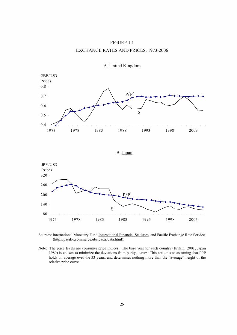
28

FIGURE 1.1

EXCHANGE RATES AND PRICES, 1973-2006

A. United Kingdom

0.4

0.5

0.6

0.7

0.8

1973 1978 1983 1988 1993 1998 2003

GBP/USD Prices

B. Japan

80

140

200

260

320

1973 1978 1983 1988 1993 1998 2003

JPY/USD Prices

Sources: International Monetary Fund International Financial Statistics, and Pacific Exchange Rate Service (http://pacific.commerce.ubc.ca/xr/data.html).

Note: The price levels are consumer price indices. The base year for each country (Britain 2001, Japan

1980) is chosen to minimize the deviations from parity, S-P/P* . This amounts to assuming that PPP holds on average over the 33 years, and determines nothing more than the “average” height of the relative price curve.

*P P

S

S

*P P

29

FIGURE 1.2

THE GROWTH OF ECONOMIC RESEARCH

Source: Factiva (http://global.factiva.com/sb/default.aspx?NAPC=S&fcpil=en). Keyword search conducted in January 2007.

30

s

E (e) = 0

-k

r1 r2 r

-k + e2

-k + e1

s

s

s0

W X

Z

Y

FIGURE 2.1

THE GEOMETRY OF PPP A. Absolute PPP

B. Relative PPP

C. Stochastic PPP

s

r

45o

r 2

s1

s2

A

r 1

B

s

r

45o

q=k Correctly priced q<k

Undervalued

q>k Overvalued

C

s

r 45o

q<0 Undervalued

q=0 Correctly priced

q>0 Overvalued

C

s

r

F

F′

D

E

k − z zkq +≤≤ Correctly priced

D′

E′ q < k − z Undervalued

zkq +> Overvalued

C

s

r

-k > 0 45o

r 2

s2

A

B

r 1

s1

31

FIGURE 3.1

EXAMPLE OF BIG MAC ARTICLE

Source: The Economist, 27 May 2006, p.70.

TABLE 3.1

IMPLIED PPP EXCHANGE RATES FOR 24 COUNTRIES, 1994 TO 2006

Country Year 1994 1995 1996 1997 1998 1999 2000 2001 2002 2003 2004 2005 2006

Mean SD CV (×100)

Argentina 1.565 1.293 1.271 1.033 0.977 1.029 0.996 0.984 1.004 1.513 1.500 1.550 2.258 1.306 0.36 27.40Australia 1.065 1.056 1.059 1.033 1.035 1.091 1.032 1.181 1.205 1.107 1.120 1.060 1.048 1.084 0.05 4.94Brazil 652.2 1.043 1.250 1.227 1.211 1.214 1.175 1.417 1.446 1.679 1.860 1.930 2.065 51.51 173.40 336.64Britain 0.787 0.750 0.758 0.748 0.719 0.782 0.757 0.783 0.799 0.734 0.649 0.613 0.626 0.731 0.06 8.22Canada 1.243 1.194 1.212 1.190 1.090 1.230 1.135 1.311 1.337 1.181 1.100 1.070 1.135 1.187 0.08 6.59Chile 412.2 409.5 402.5 495.9 488.3 514.4 502.0 496.1 562.2 516.6 483.0 490.0 503.2 482.8 45.12 9.35China 3.913 3.879 3.983 4.008 3.867 4.074 3.944 3.898 4.217 3.653 3.590 3.430 3.387 3.834 0.24 6.21Czech Republic 21.74 21.55 21.61 21.90 21.09 21.63 21.66 22.05 22.60 20.87 19.50 18.40 19.05 21.05 1.22 5.79Denmark 11.20 11.53 10.91 10.64 9.297 10.19 9.861 9.744 9.940 10.24 9.570 9.070 8.952 10.09 0.77 7.65Euro Area 1.091 1.077 1.073 1.032 0.960 1.037 1.020 1.012 1.072 1.000 0.943 0.952 0.948 1.017 0.05 5.02Hong Kong 4.000 4.095 4.195 4.091 3.984 4.198 4.064 4.213 4.498 4.244 4.140 3.920 3.871 4.116 0.16 3.80Hungary 73.48 82.33 96.79 112.0 101.2 123.0 135.1 157.1 184.3 180.8 183.0 173.0 180.6 137.1 39.83 29.05Japan 170.0 168.5 122.0 121.5 109.4 121.0 117.1 115.7 105.2 96.68 90.30 81.70 80.65 115.4 26.86 23.28Malaysia 1.639 1.621 1.593 1.599 1.680 1.860 1.801 1.780 2.024 1.860 1.740 1.720 1.774 1.745 0.12 6.84Mexico 3.522 4.698 6.314 6.157 6.992 8.189 8.327 8.622 8.795 8.487 8.280 9.150 9.355 7.453 1.73 23.23New Zealand 1.236 1.272 1.250 1.343 1.348 1.399 1.355 1.417 1.586 1.458 1.500 1.450 1.435 1.388 0.10 7.04Poland 13478 1.466 1.610 1.777 2.070 2.263 2.191 2.323 2.369 2.325 2.170 2.120 2.097 1039 3591 345.61Russia 1261 3491 4025 4545 4688 13.79 15.74 13.78 15.66 15.13 14.50 13.70 15.48 1394 1908 136.89Singapore 1.296 1.272 1.292 1.240 1.172 1.317 1.275 1.299 1.325 1.218 1.140 1.180 1.161 1.245 0.06 4.95South Korea 1000 991.4 974.6 950.4 1016 1235 1195 1181 1245 1218 1103 817.0 806.5 1056 146.03 13.83Sweden 11.09 11.21 11.02 10.74 9.375 9.877 9.562 9.449 10.44 11.07 10.30 10.10 10.65 10.37 0.63 6.08Switzerland 2.478 2.543 2.500 2.438 2.305 2.428 2.351 2.480 2.530 2.325 2.170 2.060 2.032 2.357 0.17 7.05Taiwan 26.96 28.02 27.54 28.10 26.56 28.81 27.89 27.56 28.11 25.83 25.90 24.50 24.52 26.95 1.34 4.97Thailand 20.87 20.69 20.34 19.30 20.31 21.40 21.91 21.65 22.09 21.77 20.30 19.60 19.35 20.74 0.94 4.51

Notes: 1. The implied PPP exchange rate for country c in year t is defined as *ct tP P , where ctP is the price of a Big Mac hamburger in country c during t

and *tP is the corresponding price in the US.

2. SD stands for standard deviation, and CV is the coefficient of variation.

Source: The Economist. See Appendix for details.

TABLE 3.2

NOMINAL EXCHANGE RATES FOR 24 COUNTRIES, 1994 TO 2006

Country Year 1994 1995 1996 1997 1998 1999 2000 2001 2002 2003 2004 2005 2006

Mean SD CV (×100)

Argentina 1.000 1.000 1.000 1.000 1.000 1.000 1.000 1.000 3.130 2.880 2.941 2.870 3.060 1.760 0.96 54.75Australia 1.420 1.350 1.270 1.290 1.510 1.590 1.680 1.980 1.860 1.610 1.436 1.293 1.330 1.509 0.22 14.39Brazil 949.0 0.900 0.990 1.060 1.140 1.730 1.790 2.190 2.340 3.070 3.153 2.474 2.300 74.78 252.37 337.48Britain 0.685 0.621 0.662 0.613 0.602 0.621 0.633 0.699 0.690 0.633 0.560 0.548 0.532 0.623 0.05 8.24Canada 1.390 1.390 1.360 1.390 1.420 1.510 1.470 1.560 1.570 1.450 1.375 1.244 1.120 1.404 0.12 8.37Chile 414.0 395.0 408.0 417.0 455.0 484.0 514.0 601.0 655.0 716.0 644.0 590.4 530.0 524.9 103.36 19.69China 8.700 8.540 8.331 8.330 8.280 8.280 8.280 8.280 8.280 8.280 8.349 8.366 8.030 8.333 0.15 1.78Czech Republic 29.70 26.20 27.60 29.20 34.40 35.59 39.10 39.00 34.00 28.90 26.71 24.53 22.10 30.54 5.20 17.04Denmark 6.690 5.430 5.850 6.520 7.020 6.910 8.040 8.460 8.380 6.780 6.214 6.047 5.820 6.782 0.94 13.92Euro Area 0.881 0.742 0.793 0.873 0.927 0.926 1.075 1.136 1.124 0.909 0.835 0.814 0.781 0.909 0.12 13.65Hong Kong 7.730 7.730 7.740 7.750 7.750 7.750 7.790 7.800 7.800 7.800 7.811 7.840 7.750 7.772 0.03 0.44Hungary 103.0 121.0 150.9 178.0 213.0 237.0 279.0 303.0 272.0 224.0 210.3 203.5 206.0 207.8 56.89 27.38Japan 104.0 84.20 107.0 126.0 135.0 120.0 106.0 124.0 130.0 120.0 112.9 106.1 112.0 114.4 12.95 11.32Malaysia 2.690 2.490 2.490 2.500 3.720 3.800 3.800 3.800 3.800 3.800 3.783 3.822 3.630 3.394 0.57 16.85Mexico 3.360 6.370 7.370 7.900 8.540 9.540 9.410 9.290 9.280 10.53 11.50 10.89 11.30 8.868 2.16 24.36New Zealand 1.736 1.510 1.470 1.450 1.820 1.870 2.010 2.470 2.240 1.780 1.630 1.394 1.620 1.769 0.31 17.36Poland 22433 2.340 2.640 3.100 3.460 3.980 4.300 4.030 4.040 3.890 3.875 3.312 3.100 1729 5977 345.68Russia 1775 4985 4918 5739 5999 24.70 28.50 28.90 31.20 31.10 29.00 28.54 27.10 1819 2451 134.76Singapore 1.570 1.400 1.410 1.440 1.620 1.730 1.700 1.810 1.820 1.780 1.727 1.662 1.590 1.635 0.14 8.63South Korea 810.0 769.0 779.0 894.0 1474 1218 1108 1325 1304 1220 1173 1009 952.0 1080 220.10 20.38Sweden 7.970 7.340 6.710 7.720 8.000 8.320 8.840 10.28 10.30 8.340 7.574 7.426 7.280 8.162 1.05 12.84Switzerland 1.440 1.130 1.230 1.470 1.520 1.480 1.700 1.730 1.660 1.370 1.284 1.248 1.210 1.421 0.19 13.29Taiwan 26.40 25.70 27.20 27.60 33.00 33.20 30.60 32.90 34.80 34.80 33.64 31.01 32.10 31.00 3.10 10.00Thailand 25.30 24.60 25.30 26.10 40.00 37.60 38.00 45.50 43.30 42.70 40.60 40.83 38.40 36.02 7.43 20.63

Notes: 1. The nominal exchange rate is the domestic currency cost of one US dollar. An increase thus implies a depreciation of the domestic currency and vice versa.

2. SD stands for standard deviation, and CV is the coefficient of variation.

Source: The Economist. See Appendix for details.

0

20

40

60

0 20 40 60

FIGURE 3.2

THE VOLATILITY OF EXCHANGE RATES AND PRICES

(Coefficients of variation; percentages)

0

100

200

300

400

0 100 200 300 400 Implied

PPP Implied PPP

Exchange rate

Exchange rate

Poland

Russia

Brazil

45o

45o

TABLE 3.3

REAL EXCHANGE RATES FOR 24 COUNTRIES, 1994 TO 2006

Country Year 1994 1995 1996 1997 1998 1999 2000 2001 2002 2003 2004 2005 2006

Mean SE t-value

Argentina 44.80 25.70 24.00 3.25 -2.37 2.84 -0.40 -1.59 -113.70 -64.38 -67.33 -61.62 -30.39 -18.55 12.69 -1.46 Australia -28.75 -24.56 -18.14 -22.21 -37.76 -37.71 -48.74 -51.66 -43.42 -37.46 -24.85 -19.85 -23.79 -32.22 3.11 -10.35 Brazil -37.51 14.76 23.32 14.65 6.04 -35.42 -42.07 -43.51 -48.15 -60.35 -52.76 -24.85 -10.80 -22.82 8.02 -2.84 Britain 13.89 18.86 13.57 19.81 17.66 23.02 17.90 11.36 14.74 14.86 14.84 11.33 16.26 16.01 0.93 17.13 Canada -11.14 -15.20 -11.53 -15.53 -26.46 -20.47 -25.82 -17.39 -16.04 -20.54 -22.31 -15.08 1.37 -16.63 2.01 -8.27 Chile -0.44 3.60 -1.35 17.32 7.06 6.09 -2.36 -19.19 -15.27 -32.64 -28.77 -18.63 -5.18 -6.90 4.13 -1.67 China -79.90 -78.91 -73.80 -73.15 -76.13 -70.92 -74.16 -75.35 -67.48 -81.83 -84.40 -89.16 -86.32 -77.81 1.76 -44.33 Czech Republic -31.20 -19.53 -24.47 -28.76 -48.91 -49.82 -59.06 -57.04 -40.83 -32.53 -31.47 -28.77 -14.86 -35.94 3.90 -9.23 Denmark 51.49 75.30 62.33 48.98 28.09 38.80 20.41 14.13 17.07 41.23 43.18 40.55 43.05 40.36 4.87 8.29 Euro Area 21.39 37.17 30.17 16.77 3.50 11.33 -5.28 -11.61 -4.67 9.53 12.22 15.70 19.39 11.97 3.89 3.08 Hong Kong -65.88 -63.54 -61.25 -63.89 -66.53 -61.32 -65.07 -61.60 -55.05 -60.87 -63.49 -69.31 -69.42 -63.63 1.07 -59.60 Hungary -33.77 -38.51 -44.40 -46.34 -74.45 -65.55 -72.55 -65.69 -38.90 -21.42 -13.93 -16.25 -13.13 -41.92 6.16 -6.80 Japan 49.14 69.39 13.15 -3.65 -21.05 0.82 9.99 -6.89 -21.15 -21.61 -22.31 -26.14 -32.84 -1.01 8.46 -0.12 Malaysia -49.54 -42.94 -44.65 -44.68 -79.51 -71.44 -74.68 -75.87 -62.99 -71.45 -77.65 -79.85 -71.59 -65.14 3.99 -16.32 Mexico 4.70 -30.44 -15.47 -24.93 -20.00 -15.27 -12.23 -7.46 -5.37 -21.57 -32.85 -17.44 -18.89 -16.71 2.83 -5.90 New Zealand -33.93 -17.19 -16.21 -7.67 -30.05 -29.01 -39.46 -55.54 -34.50 -19.98 -8.34 3.92 -12.09 -23.08 4.42 -5.22 Poland -50.95 -46.79 -49.44 -55.66 -51.36 -56.44 -67.41 -55.10 -53.36 -51.48 -57.98 -44.63 -39.10 -52.28 1.92 -27.28 Russia -34.20 -35.61 -20.03 -23.32 -24.67 -58.31 -59.39 -74.07 -68.91 -72.06 -69.31 -73.40 -55.97 -51.48 5.78 -8.90 Singapore -19.21 -9.62 -8.71 -14.98 -32.38 -27.29 -28.78 -33.16 -31.72 -37.96 -41.55 -34.25 -31.42 -27.00 2.93 -9.22 South Korea 21.07 25.40 22.40 6.12 -37.25 1.35 7.58 -11.50 -4.63 -0.19 -6.19 -21.07 -16.59 -1.04 5.05 -0.21 Sweden 33.01 42.32 49.58 33.05 15.86 17.15 7.85 -8.43 1.37 28.32 30.75 30.75 38.00 24.58 4.66 5.27 Switzerland 54.29 81.12 70.93 50.59 41.62 49.50 32.40 36.03 42.14 52.88 52.47 50.08 51.85 51.22 3.63 14.09 Taiwan 2.09 8.63 1.25 1.79 -21.70 -14.19 -9.28 -17.71 -21.34 -29.81 -26.14 -23.57 -26.95 -13.61 3.63 -3.75 Thailand -19.25 -17.31 -21.83 -30.20 -67.76 -56.37 -55.05 -74.25 -67.31 -67.36 -69.31 -73.40 -68.51 -52.92 6.16 -8.59 Mean -8.32 -1.58 -4.19 -10.11 -24.94 -21.61 -26.90 -31.80 -30.81 -27.44 -26.98 -24.37 -19.08 -19.86 2.86 -6.94 SE 7.83 8.73 7.61 6.79 7.04 7.29 7.03 6.64 7.01 7.53 7.75 7.70 7.40 6.77 2.10 - t-value -1.06 -0.18 -0.55 -1.49 -3.54 -2.96 -3.83 -4.79 -4.40 -3.64 -3.48 -3.16 -2.58 -2.93 - -9.47

Notes: 1. The real exchange rate for country c in year t is defined as ( )*c,t c,t c,t tq = log P S P , where c,tP is the price of a Big Mac hamburger in country c during t,

*tP is the corresponding price in the US and c,tS is the nominal exchange rate, defined as the domestic currency cost of $US1. A positive value of c,tq

implies that the domestic currency is overvalued in real terms and vice versa. 2. All entries, except those in the last row and column, are to be divided by 100. 3. SE is standard error of the mean, which is a multiple 1/ k of the corresponding standard deviation, where k=13 is the number of observations for the

row means and k=24 for the columns means. The t-values provide a test of the hypothesis that the means are zero. 4. The second to last entry in the second to last row/column is the standard error of the grand average, calculated as the standard deviation of all 24×13=312

observations divided by 312 . The corresponding t-value is presented in the right-bottom entry of the table. Source: Derived from Tables 3.1 and 3.2.

FIGURE 3.3

BIG MAC REAL EXCHANGE RATES FOR 24 COUNTRIES, 1994-2006

(Mean indicated by dashed-dotted lines; two standard-error band shaded; all × 100)

(continued on next page)

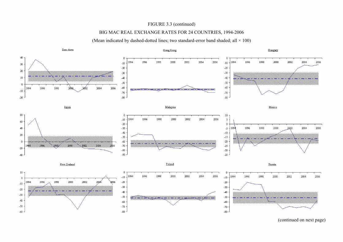
FIGURE 3.3 (continued)

BIG MAC REAL EXCHANGE RATES FOR 24 COUNTRIES, 1994-2006

(Mean indicated by dashed-dotted lines; two standard-error band shaded; all × 100)

(continued on next page)

FIGURE 3.3 (continued)

BIG MAC REAL EXCHANGE RATES FOR 24 COUNTRIES, 1994-2006

(Mean indicated by dashed-dotted lines; two standard-error band shaded; all × 100)

39

TABLE 3.4 CONTINGENCY TABLE TEST OF

SERIAL INDEPENDENCE OF MISPRICING, ONE YEAR HORIZON

Mispricing Mispricing in year t+1 in year t Undervalued Overvalued

Total

I. Observed Undervalued 192 10 202 Overvalued 14 72 86

Total 206 82 288

II. Expected under independence Undervalued 144 58 202 Overvalued 62 24 86

Total 206 82 288

III. Squared deviations Undervalued 15.6 39.3 54.9 Overvalued 36.7 92.2 128.9

Total 52.3 131.5 183.8

Note: The (i, j)th element of Panel III is 2ij ij ij(O E ) / E− , where ijO

and ijE are the corresponding observed and expected values.

TABLE 3.5 TESTS OF SERIAL INDEPENDENCE

OVER VARIOUS HORIZONS

Observed 2χ value, with overlapping observations Horizon

(Years) Included Excluded

1 183.8 183.8 2 142.2 75.7 3 104.4 41.6 4 82.1 24.1 5 68.4 23.5 6 54.9 18.0 7 43.5 4.8 8 37.8 6.7 9 27.1 8.8

10 18.5 8.8 11 10.2 5.7 12 5.7 5.7

Notes: Under the null of independence, the test statistic follows a 2χ distribution with 1 degree of freedom. The critical value of ( )2

.05χ 1 is 3.8 and ( )2.01χ 1 is 6.6.

40

TABLE 3.6

RUNS TESTS FOR ABSOLUTE PARITY

Number of runs Country Sequence of signs of disparities Observed R Expected

( )E R

Standard deviation

var R

Test statistic

Z

Argentina + + + + − + − − − − − − − 4 7.15 1.63 -1.94 Australia − − − − − − − − − − − − − 1 1.00 0.00 +∞ Brazil − + + + + − − − − − − − − 3 6.54 1.45 -2.44 Britain + + + + + + + + + + + + + 1 1.00 0.00 +∞ Canada − − − − − − − − − − − − + 2 2.85 0.36 -2.35 Chile − + − + + + − − − − − − − 4 6.54 1.45 -1.75 China − − − − − − − − − − − − − 1 1.00 0.00 +∞ Czech Republic − − − − −− − − − − −− − 1 1.00 0.00 +∞ Denmark + + + + + + + + + + + + + 1 1.00 0.00 +∞ Euro Area + + + + + + − − − + + + + 3 5.62 1.18 -2.22 Hong Kong − − − − −− − − − − −− − 1 1.00 0.00 +∞ Hungary − − − − − − − − − − − − − 1 1.00 0.00 +∞ Japan + + + − − + + − − − − − − 4 7.15 1.63 -1.94 Malaysia − − − − −− − − − − −− − 1 1.00 0.00 +∞ Mexico + − − − − − − − − − − − − 2 2.85 0.36 -2.35 New Zealand − − − − − − − − − − − − + 2 2.85 0.36 -2.35 Poland − − − − −− − − − − −− − 1 1.00 0.00 +∞ Russia − − − − −− − − − − −− − 1 1.00 0.00 +∞ Singapore − − − − − − − − − − − − − 1 1.00 0.00 +∞ South Korea + + + + − + + − − − − − − 4 7.46 1.71 -2.02 Sweden + + + + + + + − + + + + + 2 2.85 0.36 -2.35 Switzerland + + + + + + + + + + + + + 1 1.00 0.00 +∞ Taiwan + + + + − − − − − − − − − 2 6.54 1.45 -3.14 Thailand − − − − −− − − − − −− − 1 1.00 0.00 +∞

FIGURE 3.4

THE GEOGRAPHY OF MONEY

OVER/UNDER-VALUATION OF CURRENCIES, 1994-2006 AVERAGES

-100

-80

-60

-40

-20

0

20

40

60

Bra

zil

Arg

entin

a

Mex

ico

Can

ada

Chi

le

Pola

nd

Rus

sia

Hun

gary

Cze

ch R

epub

lic

Euro

Are

a

Brit

ain

Swed

en

Den

mar

k

Switz

erla

nd

Aus

tralia

New

Zea

land

Chi

na

Mal

aysi

a

Hon

g K

ong

Thai

land

Sing

apor

e

Taiw

an

Sout

h K

orea

The Americas Europe Oceania Asia

Mean Real Exchange Rate

( 100)× O

verv

alua

tion

Und

erva

luat

ion

Grand Average

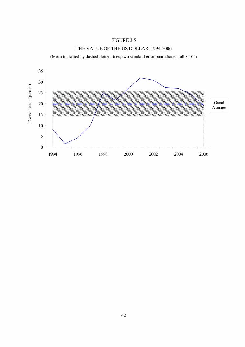
42

FIGURE 3.5

THE VALUE OF THE US DOLLAR, 1994-2006

(Mean indicated by dashed-dotted lines; two standard error band shaded; all × 100)

0

5

10

15

20

25

30

35

1994 1996 1998 2000 2002 2004 2006

Ove

rval

uatio

n (p

erce

nt)

Grand Average

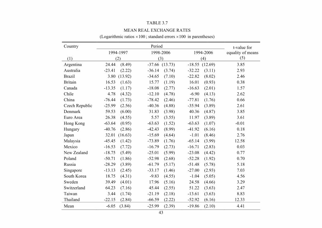
43

TABLE 3.7

MEAN REAL EXCHANGE RATES (Logarithmic ratios 100× ; standard errors 100× in parentheses)

Country Period 1994-1997 1998-2006 1994-2006

t-value for equality of means

(1) (2) (3) (4) (5) Argentina 24.44 (8.49) -37.66 (13.73) -18.55 (12.69) 3.85 Australia -23.41 (2.22) -36.14 (3.74) -32.22 (3.11) 2.93 Brazil 3.80 (13.92) -34.65 (7.10) -22.82 (8.02) 2.46 Britain 16.53 (1.63) 15.77 (1.19) 16.01 (0.93) 0.38 Canada -13.35 (1.17) -18.08 (2.77) -16.63 (2.01) 1.57 Chile 4.78 (4.32) -12.10 (4.78) -6.90 (4.13) 2.62 China -76.44 (1.73) -78.42 (2.46) -77.81 (1.76) 0.66 Czech Republic -25.99 (2.56) -40.36 (4.88) -35.94 (3.89) 2.61 Denmark 59.53 (6.00) 31.83 (3.98) 40.36 (4.87) 3.85 Euro Area 26.38 (4.55) 5.57 (3.55) 11.97 (3.89) 3.61 Hong Kong -63.64 (0.95) -63.63 (1.52) -63.63 (1.07) -0.01 Hungary -40.76 (2.86) -42.43 (8.99) -41.92 (6.16) 0.18 Japan 32.01 (16.63) -15.69 (4.64) -1.01 (8.46) 2.76 Malaysia -45.45 (1.42) -73.89 (1.76) -65.14 (3.99) 12.58 Mexico -16.53 (7.72) -16.79 (2.73) -16.71 (2.83) 0.03 New Zealand -18.75 (5.49) -25.01 (5.99) -23.08 (4.42) 0.77 Poland -50.71 (1.86) -52.98 (2.68) -52.28 (1.92) 0.70 Russia -28.29 (3.89) -61.79 (5.17) -51.48 (5.78) 5.18 Singapore -13.13 (2.45) -33.17 (1.46) -27.00 (2.93) 7.03 South Korea 18.75 (4.31) -9.83 (4.55) -1.04 (5.05) 4.56 Sweden 39.49 (4.01) 17.96 (5.16) 24.58 (4.66) 3.29 Switzerland 64.23 (7.16) 45.44 (2.55) 51.22 (3.63) 2.47 Taiwan 3.44 (1.74) -21.19 (2.18) -13.61 (3.63) 8.83 Thailand -22.15 (2.84) -66.59 (2.22) -52.92 (6.16) 12.33 Mean -6.05 (3.84) -25.99 (2.39) -19.86 (2.10) 4.41

44

FIGURE 4.1

SCATTER PLOTS OF EXCHANGE RATES AND PRICES, 24 COUNTRIES, 1994-2006

(Annualised logarithmic changes 100× )

1-year Horizon

-100

-80

-60

-40

-20

0

20

40

60

80

100

-100 -80 -60 -40 -20 0 20 40 60 80 100

Exchange Rate

Inflation

RMSE = 14.39%

2-year Horizon

-100

-80

-60

-40

-20

0

20

40

60

80

100

-100 -80 -60 -40 -20 0 20 40 60 80 100

Exchange Rate

Inflation

RMSE = 9.70%

3-year Horizon

-100

-80

-60

-40

-20

0

20

40

60

80

100

-100 -80 -60 -40 -20 0 20 40 60 80 100

Exchange Rate

Inflation

RMSE = 7.84%

4-year Horizon

-100

-80

-60

-40

-20

0

20

40

60

80

100

-100 -80 -60 -40 -20 0 20 40 60 80 100

Exchange Rate

Inflation

RMSE = 6.73%

(continued on next page)

45

FIGURE 4.1 (continued)

SCATTER PLOTS OF EXCHANGE RATES AND PRICES, 24 COUNTRIES, 1994-2006

(Annualised logarithmic changes 100× )

5-year Horizon

-100

-80

-60

-40

-20

0

20

40

60

80

100

-100 -80 -60 -40 -20 0 20 40 60 80 100

Exchange Rate

Inflation

RMSE = 5.63%

6-year Horizon

-100

-80

-60

-40

-20

0

20

40

60

80

100

-100 -80 -60 -40 -20 0 20 40 60 80 100

Exchange Rate

Inflation

RMSE = 5.03%

7-year Horizon

-100

-80

-60

-40

-20

0

20

40

60

80

100

-100 -80 -60 -40 -20 0 20 40 60 80 100

Exchange Rate

Inflation

RMSE = 4.45%

8-year Horizon

-100

-80

-60

-40

-20

0

20

40

60

80

100

-100 -80 -60 -40 -20 0 20 40 60 80 100

Exchange Rate

Inflation

RMSE = 4.07%

(continued on next page)

46

FIGURE 4.1 (continued)

SCATTER PLOTS OF EXCHANGE RATES AND PRICES, 24 COUNTRIES, 1994-2006

(Annualised logarithmic changes 100× )

9-year Horizon

-100

-80

-60

-40

-20

0

20

40

60

80

100

-100 -80 -60 -40 -20 0 20 40 60 80 100

Exchange Rate

Inflation

RMSE = 3.49%

10-year Horizon

-100

-80

-60

-40

-20

0

20

40

60

80

100

-100 -80 -60 -40 -20 0 20 40 60 80 100

Exchange Rate

Inflation

RMSE = 3.27%

11-year Horizon

-100

-80

-60

-40

-20

0

20

40

60

80

100

-100 -80 -60 -40 -20 0 20 40 60 80 100

Exchange Rate

Inflation

RMSE = 3.14%

12-year Horizon

-100

-80

-60

-40

-20

0

20

40

60

80

100

-100 -80 -60 -40 -20 0 20 40 60 80 100

Exchange Rate

Inflation

RMSE = 2.47%

Notes: 1. To facilitate presentation, the cases in which the annualised logarithmic changes ( 100× ) exceeded 100% have been omitted. These cases are included in the computation of the RMSEs.

2. The dark dots refer to the 9 European countries, while the lighter ones refer to the other countries.

47

FIGURE 4.2

BLOW-UP OF SCATTER PLOTS OF EXCHANGE RATES AND PRICES, 24 COUNTRIES, 1994-2006

(Annualised logarithmic changes 100× )

1-year Horizon

-100

-80

-60

-40

-20

0

20

40

60

80

100

-100 -80 -60 -40 -20 0 20 40 60 80 100

Exchange Rate

Inflation

RMSE = 14.39%

1-year Horizon

-20

-15

-10

-5

0

5

10

15

20

-20 -15 -10 -5 0 5 10 15 20

Exchange Rate

Inflation

RMSE = 14.39%

6-year Horizon

-100

-80

-60

-40

-20

0

20

40

60

80

100

-100 -80 -60 -40 -20 0 20 40 60 80 100

Exchange Rate

Inflation

RMSE = 5.03%

6-year Horizon

-20

-15

-10

-5

0

5

10

15

20

-20 -15 -10 -5 0 5 10 15 20

Exchange Rate

Inflation

RMSE = 5.03%

(continued on next page)

48

FIGURE 4.2 (continued)

BLOW-UP OF SCATTER PLOTS OF EXCHANGE RATES AND PRICES, FOR 24 COUNTRIES, 1994-2006

(Annualised logarithmic changes 100× )

12-year Horizon

-100

-80

-60

-40

-20

0

20

40

60

80

100

-100 -80 -60 -40 -20 0 20 40 60 80 100

Exchange Rate

Inflation

RMSE = 2.47%

12-year Horizon

-20

-15

-10

-5

0

5

10

15

20

-20 -15 -10 -5 0 5 10 15 20

Exchange Rate

Inflation

RMSE = 2.47%

Notes: 1.To facilitate presentation, the cases in which the annualised logarithmic changes ( 100× ) exceeded 20% have been omitted. These cases are included in the computation of the RMSEs.

2. The dark dots refer to the 9 European countries, while the lighter ones refer to the other countries.

49

FIGURE 4.3

VARIANCES OF EXCHANGE RATE CHANGES

A. Annualised changes B. Total changes

1 2 3 4 5 6 7 8 9 10 11 12

Stationary

Non-stationary

1 2 3 4 5 6 7 8 9 10 11 12

Stationary

Non-stationary

FIGURE 4.4

TOTAL VOLATILITY AND THE HORIZON

0

10

20

30

40

0 2 4 6 8 10 12

(h)tvar q⎡ ⎤Δ⎣ ⎦

22

1εσ

+β

Horizon h

A

(h) tvar q⎡ ⎤Δ⎣ ⎦

Horizon h

Standard deviation

(h×RMSE×100)

Horizon

50

FIGURE 5.1

SCATTER PLOTS OF FUTURE REAL EXCHANGE RATES AGAINST CURRENT DEVIATIONS FROM PARITY, 24 COUNTRIES, 1994-2006

(Logarithmic changes 100× )

1-year Horizon

-80

-60

-40

-20

0

20

40

60

80

-40 -30 -20 -10 0 10 20 30 40dc,t

Chi Square = 12.56

y = -0.92 -0.35x (0.76) (0.04)

qc,t+1 - qc,t

2-year Horizon

-80

-60

-40

-20

0

20

40

60

80

-40 -30 -20 -10 0 10 20 30 40

dc,t

Chi Square = 22.39

y = -2.83 -0.66x (0.93) (0.05)

qc,t+2 - qc,t

3-year Horizon

-80

-60

-40

-20

0

20

40

60

80

-40 -30 -20 -10 0 10 20 30 40

dc,t

Chi Square = 34.42

y = -4.63 -0.93x (1.00) (0.05)

qc,t+3 - qc,t

4-year Horizon

-80

-60

-40

-20

0

20

40

60

80

-40 -30 -20 -10 0 10 20 30 40

dc,t

Chi Square = 78.21

y = -5.84 -1.14x (1.01) (0.05)

qc,t+4 - qc,t

(continued on next page)

51

FIGURE 5.1 (continued)

SCATTER PLOTS OF FUTURE REAL EXCHANGE RATES AGAINST CURRENT DEVIATIONS FROM PARITY, 24 COUNTRIES, 1994-2006

(Logarithmic changes 100× )

5-year Horizon

-80

-60

-40

-20

0

20

40

60

80

-40 -30 -20 -10 0 10 20 30 40

dc,t

Chi Square = 101.01

y = -5.28 -1.27x (1.05) (0.06)

qc,t+5 - qc,t

6-year Horizon

-80

-60

-40

-20

0

20

40

60

80

-40 -30 -20 -10 0 10 20 30 40dc,t

Chi Square = 93.86

y = -4.63 -1.39x (1.16) (0.06)

qc,t+6 - qc,t

7-year Horizon

-80

-60

-40

-20

0

20

40

60

80

-40 -30 -20 -10 0 10 20 30 40

dc,t

Chi Square = 70.23

y = -3.73 -1.39x (1.36) (0.07)

qc,t+7 - qc,t

8-year Horizon

-80

-60

-40

-20

0

20

40

60

80

-40 -30 -20 -10 0 10 20 30 40

dc,t

Chi Square = 47.33

y = -1.50 -1.44x (1.56) (0.08)

qc,t+8 - qc,t

(continued on next page)

52

FIGURE 5.1 (continued)

SCATTER PLOTS OF FUTURE REAL EXCHANGE RATES AGAINST CURRENT DEVIATIONS FROM PARITY, 24 COUNTRIES, 1994-2006

(Logarithmic changes 100× )

9-year Horizon

-80

-60

-40

-20

0

20

40

60

80

-40 -30 -20 -10 0 10 20 30 40

dc,t

Chi Square = 13.96

y = 0.92 -1.40x (1.89) (0.09)

qc,t+9 - qc,t

10-year Horizon

-80

-60

-40

-20

0

20

40

60

80

-40 -30 -20 -10 0 10 20 30 40dc,t

Chi Square = 10.57

y = 2.54 -1.41x (2.21) (0.10)

qc,t+10 - qc,t

11-year Horizon

-80

-60

-40

-20

0

20

40

60

80

-40 -30 -20 -10 0 10 20 30 40

dc,t

Chi Square = 1.03

y = 5.10 -1.47x (2.33) (0.10)

qc,t+11 - qc,t

12-year Horizon

-80

-60

-40

-20

0

20

40

60

80

-40 -30 -20 -10 0 10 20 30 40dc,t

Chi Square = 1.36

y = 6.41 -1.49x (2.70) (0.13)

qc,t+12 - qc,t

Note: 1. To facilitate presentation, the cases in which the annualised logarithmic changes ( 100× ) exceeded 80% have been omitted.

These cases are included in the regression and the chi square value.

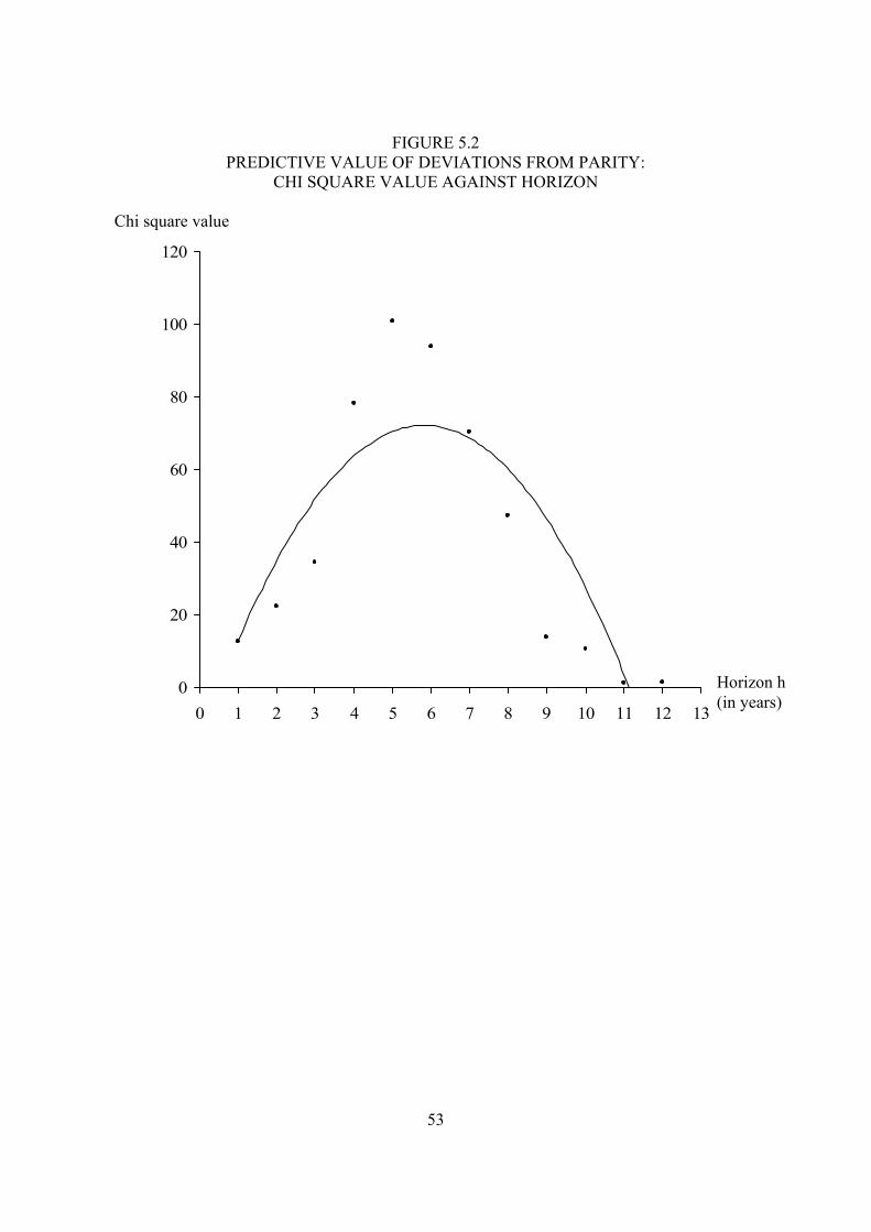
53

FIGURE 5.2 PREDICTIVE VALUE OF DEVIATIONS FROM PARITY:

CHI SQUARE VALUE AGAINST HORIZON

0

20

40

60

80

100

120

0 1 2 3 4 5 6 7 8 9 10 11 12 13

Chi square value

Horizon h (in years)

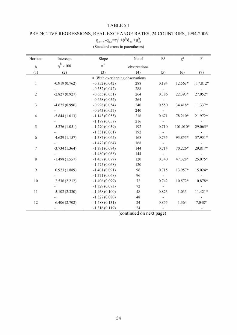
54

TABLE 5.1

PREDICTIVE REGRESSIONS, REAL EXCHANGE RATES, 24 COUNTRIES, 1994-2006 h h h

c,t+h c,t c,t c,tq -q = + d +uη φ (Standard errors in parentheses)

Horizon Intercept Slope No of R² χ² F

h hη 100× hφ observations

(1) (2) (3) (4) (5) (6) (7) A. With overlapping observations

1 -0.919 (0.762) -0.352 (0.042) 288 0.194 12.563* 117.812* - -0.352 (0.042) 288 - -

2 -2.827 (0.927) -0.655 (0.051) 264 0.386 22.393* 27.052* - -0.658 (0.052) 264 - -

3 -4.625 (0.996) -0.928 (0.054) 240 0.550 34.418* 11.337* - -0.943 (0.057) 240 - -

4 -5.844 (1.013) -1.143 (0.055) 216 0.671 78.210* 21.972* - -1.178 (0.058) 216 - -

5 -5.276 (1.051) -1.270 (0.059) 192 0.710 101.010* 29.065* - -1.331 (0.061) 192 - -

6 -4.629 (1.157) -1.387 (0.065) 168 0.735 93.855* 37.951* - -1.472 (0.064) 168 - -

7 -3.734 (1.364) -1.391 (0.074) 144 0.714 70.226* 29.817* - -1.480 (0.068) 144 - -

8 -1.498 (1.557) -1.437 (0.079) 120 0.740 47.328* 25.075* - -1.475 (0.068) 120 - -

9 0.923 (1.889) -1.401 (0.091) 96 0.715 13.957* 15.024* - -1.371 (0.068) 96 - -

10 2.536 (2.212) -1.406 (0.099) 72 0.742 10.572* 10.878* - -1.329 (0.073) 72 - -

11 5.102 (2.330) -1.468 (0.100) 48 0.823 1.033 11.421* - -1.327 (0.080) 48 - -

12 6.406 (2.702) -1.488 (0.131) 24 0.855 1.364 7.048* - -1.316 (0.119) 24 - -

(continued on next page)

55

TABLE 5.1 (continued)

PREDICTIVE REGRESSIONS, REAL EXCHANGE RATES, 24 COUNTRIES, 1994-2006

Horizon Intercept Slope No of R² χ² F

h hη 100× hφ observations

(1) (2) (3) (4) (5) (6) (7) B. Without overlapping observations

1 -0.919 (0.762) -0.352 (0.042) 288 0.194 12.563* 117.812* - -0.352 (0.042) 288 - - -

2 -2.130 (1.375) -0.673 (0.073) 144 0.373 12.355* 11.324* - -0.670 (0.074) 144 - - -

3 -1.187 (1.509) -0.904 (0.091) 96 0.514 19.703* 0.795 - -0.911 (0.090) 96 - - -

4 -5.246 (2.050) -1.106 (0.102) 72 0.628 23.074* 3.639* - -1.087 (0.105) 72 - - -

5 -4.643 (1.973) -0.958 (0.124) 48 0.565 19.368* 2.851 - -1.047 (0.123) 48 - - -

6 -2.846 (1.970) -1.129 (0.111) 48 0.691 30.857* 1.960 - -1.149 (0.112) 48 - - -

7 -15.246 (3.000) -0.713 (0.145) 24 0.524 8.291* 13.447* - -1.124 (0.174) 24 - - -

8 -2.773 (4.186) -1.709 (0.202) 24 0.764 13.029* 11.116* - -1.784 (0.166) 24 - - -

9 -3.228 (3.237) -1.378 (0.156) 24 0.779 8.539* 6.907* - -1.465 (0.130) 24 - - -

10 -1.370 (3.257) -1.499 (0.157) 24 0.805 5.874* 8.491* - -1.536 (0.128) 24 - - -

11 2.991 (2.722) -1.651 (0.132) 24 0.877 0.758 14.234* - -1.570 (0.110) 24 - - -

12 6.406 (2.702) -1.488 (0.131) 24 0.855 1.364 7.048* - -1.316 (0.119) 24 - - -

Notes: 1. The2

χ statistics of column 6 test the hypothesis of the independence of q q

c,t+h c,t- and c,td . Under the null,

2χ has 1

degree of freedom. 2. The F statistics of column 7 test the joint hypothesis of

h=0η and

h =-1φ . Under the null, F has degrees of freedom equal to 2 and N-2, where N is the number of observations.

3. An asterisk (*) indicates significant at the 5 percent level.

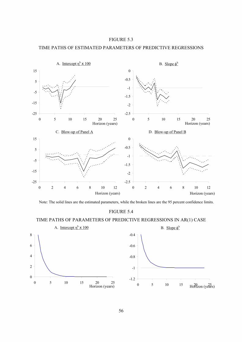
56

FIGURE 5.3

TIME PATHS OF ESTIMATED PARAMETERS OF PREDICTIVE REGRESSIONS

A. Intercept ηh x 100 B. Slope φh

-25

-15

-5

5

15

0 5 10 15 20 25

-2.5

-2

-1.5

-1

-0.5

0

0 5 10 15 20 25

C. Blow-up of Panel A D. Blow-up of Panel B

-25

-15

-5

5

15

0 2 4 6 8 10 12

-2.5

-2

-1.5

-1

-0.5

0

0 2 4 6 8 10 12

Note: The solid lines are the estimated parameters, while the broken lines are the 95 percent confidence limits.

FIGURE 5.4

TIME PATHS OF PARAMETERS OF PREDICTIVE REGRESSIONS IN AR(1) CASE A. Intercept ηh x 100 B. Slope φh

0

2

4

6

8

0 5 10 15 20 25

-1.2

-1

-0.8

-0.6

-0.4

0 5 10 15 20 25

Horizon (years) Horizon (years)

Horizon (years)Horizon (years)

Horizon (years) Horizon (years)

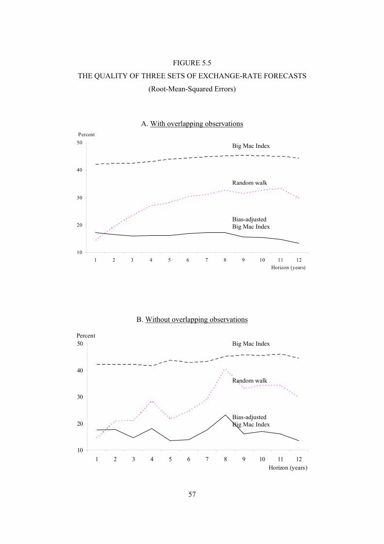
57

FIGURE 5.5

THE QUALITY OF THREE SETS OF EXCHANGE-RATE FORECASTS

(Root-Mean-Squared Errors)

A. With overlapping observations

10

20

30

40

50

1 2 3 4 5 6 7 8 9 10 11 12Horizon (years)

Percent

B. Without overlapping observations

10

20

30

40

50

1 2 3 4 5 6 7 8 9 10 11 12Horizon (years)

Percent

Random walk

Bias-adjusted Big Mac Index

Big Mac Index

Random walk

Bias-adjusted Big Mac Index

Big Mac Index

TABLE 6.1

MORE PREDICTIVE REGRESSIONS, 24 COUNTRIES, 1994-2006

(Standard errors in parentheses)

(i) Negative change in nominal exchange rate (ii) Inflation differential h h h

c,t+h c,t s s ct s,ct- )-(s s =η + d +uφ h h h hc,t+h c,t r r ct r,ct=η + d +ur -r φ

Horizon Intercept Slope No of R² χ² Intercept Slope No of R² χ²

h hsη ×100 h

sφ observations hrη ×100 h

rφ observations (1) (2) (3) (4) (5) (6) (7) (8) (9) (10) (11)

A. With overlapping observations

1 5.603 (4.511) -0.123 (0.251) 288 0.001 1.343 -6.522 (4.408) -0.229 (0.245) 288 0.003 7.660 - -0.124 (0.251) 288 - - -0.227 (0.245) 288 -

2 6.045 (5.343) -0.207 (0.294) 264 0.002 8.727 -8.873 (5.217) -0.449 (0.287) 264 0.009 8.038 - -0.200 (0.294) 264 - - -0.458 (0.288) 264 -

3 6.500 (6.292) -0.245 (0.344) 240 0.002 21.502 -11.125 (6.184) -0.683 (0.338) 240 0.017 1.968 - -0.224 (0.344) 240 - - -0.720 (0.339) 240 -

4 7.461 (7.434) -0.347 (0.402) 216 0.003 44.172 -13.305 (7.307) -0.795 (0.395) 216 0.019 0.101 - -0.303 (0.399) 216 - - -0.875 (0.394) 216 -

5 9.732 (8.639) -0.428 (0.484) 192 0.004 41.741 -15.009 (8.618) -0.842 (0.483) 192 0.016 0.224 - -0.316 (0.474) 192 - - -1.015 (0.475) 192 -

6 11.027 (10.177) -0.561 (0.568) 168 0.006 42.624 -15.655 (10.243) -0.826 (0.572) 168 0.012 0.193 - -0.358 (0.537) 168 - - -1.114 (0.542) 168 -

7 14.509 (12.398) -0.683 (0.671) 144 0.007 25.299 -18.244 (12.506) -0.708 (0.677) 144 0.008 1.389 - -0.340 (0.605) 144 - - -1.139 (0.612) 144 -

8 21.578 (15.410) -0.850 (0.777) 120 0.010 26.138 -23.076 (15.581) -0.587 (0.786) 120 0.005 0.049 - -0.300 (0.673) 120 - - -1.175 (0.681) 120 -

9 35.426 (20.626) -1.466 (0.996) 96 0.023 7.484 -34.502 (21.007) 0.065 (1.015) 96 0.000 0.269 - -0.325 (0.750) 96 - - -1.046 (0.763) 96 -

10 51.533 (25.606) -2.029 (1.148) 72 0.043 3.733 -48.997 (26.223) 0.623 (1.176) 72 0.004 0.429 - -0.458 (0.860) 72 - - -0.870 (0.877) 72 -

11 74.744 (33.705) -2.810 (1.451) 48 0.075 2.987 -69.642 (34.129) 1.342 (1.470) 48 0.018 0.009 - -0.744 (1.158) 48 - - -0.582 (1.164) 48 -

12 119.198 (55.326) -4.498 (2.674) 24 0.114 1.698 -112.792 (55.255) 3.009 (2.671) 24 0.055 0.084 - -1.287 (2.389) 24 - - -0.029 (2.365) 24 -

(continued on next page)

TABLE 6.1 (continued)

MORE PREDICTIVE REGRESSIONS, 24 COUNTRIES, 1994-2006

(Standard errors in parentheses)

(i) Negative change in nominal exchange rate (ii) Inflation differential h h h

c,t+h c,t s s ct s,ct- )-(s s =η + d +uφ

h h h hc,t+h c,t r r ct r,ct=η + d +ur -r φ

Horizon Intercept Slope No of R² χ² Intercept Slope No of R² χ²

h hsη ×100 h

sφ observations hrη ×100 h

rφ observations (1) (2) (3) (4) (5) (6) (7) (8) (9) (10) (11)

B. Without overlapping observations

1 5.603 (4.511) -0.123 (0.251) 288 0.001 1.343 -6.522 (4.408) -0.229 (0.245) 288 0.003 7.660 - -0.124 (0.251) 288 - - -0.227 (0.245) 288 - 2 11.087 (8.912) -0.269 (0.475) 144 0.002 3.334 -13.217 (8.669) -0.404 (0.462) 144 0.005 9.017 - -0.285 (0.476) 144 - - -0.386 (0.464) 144 - 3 17.733 (13.229) -0.542 (0.795) 96 0.005 5.783 -18.920 (13.005) -0.362 (0.781) 96 0.002 2.597 - -0.435 (0.794) 96 - - -0.476 (0.782) 96 - 4 21.921 (17.500) -0.349 (0.870) 72 0.002 7.276 -27.167 (17.166) -0.758 (0.853) 72 0.011 0.629 - -0.430 (0.871) 72 - - -0.657 (0.860) 72 - 5 37.162 (25.496) -1.588 (1.601) 48 0.021 11.622 -41.804 (25.494) 0.630 (1.600) 48 0.003 0.022 - -0.872 (1.541) 48 - - -0.175 (1.550) 48 - 6 36.518 (24.186) -1.272 (1.365) 48 0.019 16.326 -39.364 (24.561) 0.143 (1.386) 48 0.000 0.167 - -1.011 (1.372) 48 - - -0.139 (1.398) 48 - 7 90.569 (56.799) -3.373 (2.745) 24 0.064 1.407 -105.816 (56.558) 2.660 (2.734) 24 0.041 0.873 - -0.933 (2.354) 24 - - -0.191 (2.390) 24 - 8 96.846 (55.734) -4.258 (2.694) 24 0.102 2.476 -99.619 (56.782) 2.548 (2.744) 24 0.038 0.505 - -1.649 (2.333) 24 - - -0.136 (2.379) 24 - 9 102.990 (54.605) -4.233 (2.639) 24 0.105 2.906 -106.218 (55.870) 2.855 (2.700) 24 0.048 0.017 - -1.458 (2.310) 24 - - -0.007 (2.366) 24 -

10 108.263 (54.282) -4.290 (2.624) 24 0.108 2.274 -109.633 (55.682) 2.791 (2.691) 24 0.047 0.126 - -1.374 (2.315) 24 - - -0.162 (2.370) 24 -

11 115.903 (54.983) -4.413 (2.657) 24 0.111 1.698 -112.912 (55.574) 2.762 (2.686) 24 0.046 0.003 - -1.291 (2.366) 24 - - -0.280 (2.377) 24 -

12 119.198 (55.326) -4.498 (2.674) 24 0.114 1.698 -112.792 (55.255) 3.009 (2.671) 24 0.055 0.084 - -1.287 (2.389) 24 - - -0.029 (2.365) 24 -

Notes: The χ² statistics in columns 6 and 11 test the hypotheses of the independence between c,t+h c,t- )-(s s and ctd , and c,t+h c,tr -r and ctd , respectively. Under the null, χ² has 1 degree of freedom.

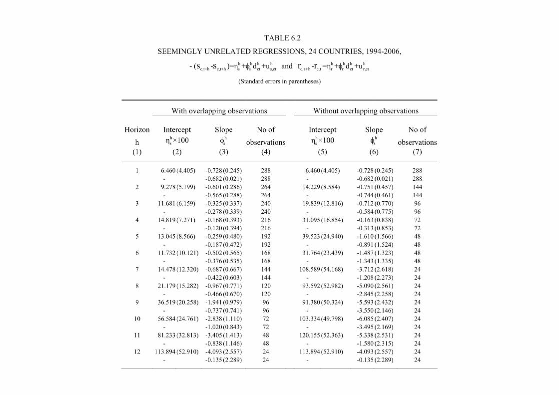
TABLE 6.2

SEEMINGLY UNRELATED REGRESSIONS, 24 COUNTRIES, 1994-2006, h h h h

c,t+h c,t+h s s ct s,ct- ( - )=η + d +us s φ and h h h hc,t+h c,t r r ct r,ct- =η + d +ur r φ

(Standard errors in parentheses)

With overlapping observations Without overlapping observations Horizon Intercept Slope No of Intercept Slope No of

h hsη ×100 h

sφ observations hsη ×100 h

sφ observations(1) (2) (3) (4) (5) (6) (7)

1 6.460 (4.405) -0.728 (0.245) 288 6.460 (4.405) -0.728 (0.245) 288 - -0.682 (0.021) 288 - -0.682 (0.021) 288 2 9.278 (5.199) -0.601 (0.286) 264 14.229 (8.584) -0.751 (0.457) 144 - -0.565 (0.288) 264 - -0.744 (0.461) 144 3 11.681 (6.159) -0.325 (0.337) 240 19.839 (12.816) -0.712 (0.770) 96 - -0.278 (0.339) 240 - -0.584 (0.775) 96 4 14.819 (7.271) -0.168 (0.393) 216 31.095 (16.854) -0.163 (0.838) 72 - -0.120 (0.394) 216 - -0.313 (0.853) 72 5 13.045 (8.566) -0.259 (0.480) 192 39.523 (24.940) -1.610 (1.566) 48 - -0.187 (0.472) 192 - -0.891 (1.524) 48 6 11.732 (10.121) -0.502 (0.565) 168 31.764 (23.439) -1.487 (1.323) 48 - -0.376 (0.535) 168 - -1.343 (1.335) 48 7 14.478 (12.320) -0.687 (0.667) 144 108.589 (54.168) -3.712 (2.618) 24 - -0.422 (0.603) 144 - -1.208 (2.273) 24 8 21.179 (15.282) -0.967 (0.771) 120 93.592 (52.982) -5.090 (2.561) 24 - -0.466 (0.670) 120 - -2.845 (2.258) 24 9 36.519 (20.258) -1.941 (0.979) 96 91.380 (50.324) -5.593 (2.432) 24 - -0.737 (0.741) 96 - -3.550 (2.146) 24

10 56.584 (24.761) -2.838 (1.110) 72 103.334 (49.798) -6.085 (2.407) 24 - -1.020 (0.843) 72 - -3.495 (2.169) 24

11 81.233 (32.813) -3.405 (1.413) 48 120.155 (52.363) -5.338 (2.531) 24 - -0.838 (1.146) 48 - -1.580 (2.315) 24

12 113.894 (52.910) -4.093 (2.557) 24 113.894 (52.910) -4.093 (2.557) 24 - -0.135 (2.289) 24 - -0.135 (2.289) 24

61

FIGURE 6.1

IMPLICATIONS OF MISPRICING

Subsequent change in nominal rate (H) t Hs +Δ

0td > •

E •

•0td− <

• E′

F

F

O

O

U

U

Subsequent inflation t+Hr(H)Δ

(Currently overvalued)

(Currently undervalued)

45o

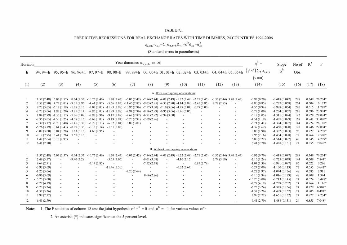
TABLE 7.1

PREDICTIVE REGRESSIONS FOR REAL EXCHANGE RATES WITH TIME DUMMIES, 24 COUNTRIES,1994-2006 h h

, h ,tc,t+h c,t c,t c,tDq -q = + d +uτ τ τ+ τ∑ α φ

(Standard errors in parentheses)

Horizon Year dummies , hτ τ+α ( 100)× hη = Slope No of R2 F

h 94, 94+h 95, 95+h 96, 96+h 97, 97+h 98, 98+h 99, 99+h 00, 00+h 01, 01+h 02, 02+h 03, 03+h 04, 04+h 05, 05+h ( )hτ τ,τ+h1 N α∑ hφ Obs.

( )100× (1) (2) (3) (4) (5) (6) (7) (8) (9) (10) (11) (12) (13) (14) (15) (16) (17) (18)

A. With overlapping observations

1 11.57 (2.48) 5.03 (2.57) 0.64 (2.53) -10.75 (2.46) 1.20 (2.43) -6.03 (2.42) -7.84 (2.44) -4.01 (2.49) -1.22 (2.48) -2.71 (2.45) -0.37 (2.44) 3.40 (2.43) -0.92 (0.70) -0.418 (0.047) 288 0.349 76.234* 2 12.52 (2.90) 4.77 (3.01) -9.35 (2.96) -4.41 (2.87) -5.66 (2.83) -11.46 (2.82) -9.03 (2.85) -4.33 (2.90) -4.14 (2.89) -2.45 (2.85) 2.72 (2.85) - -2.80 (0.85) -0.727 (0.058) 264 0.504 16.173* 3 9.73 (3.05) -5.12 (3.19) -1.78 (3.13) -7.07 (3.03) -11.93 (2.98) -10.95 (2.96) -7.57 (3.00) -7.10 (3.06) -4.49 (3.04) 0.79 (3.00) - - -4.55 (0.94) -0.998 (0.064) 240 0.615 11.787* 4 -2.73 (3.06) 1.97 (3.20) -3.85 (3.14) -9.95 (3.03) -11.99 (2.98) -7.94 (2.96) -8.56 (2.99) -6.95 (3.06) -1.46 (3.05) - - - -5.72 (1.00) -1.204 (0.067) 216 0.696 23.974* 5 1.84 (2.99) -1.35 (3.17) -7.06 (3.09) -7.92 (2.96) -9.17 (2.89) -7.67 (2.87) -6.71 (2.92) -2.94 (3.00) - - - - -5.12 (1.05) -1.311 (0.074) 192 0.728 28.024* 6 -2.35 (3.05) -4.50 (3.25) -4.58 (3.16) -3.62 (3.01) -9.19 (2.94) -5.23 (2.91) -2.09 (2.96) - - - - - -4.51 (1.19) -1.407 (0.079) 168 0.741 33.090* 7 -7.39 (3.17) -3.75 (3.40) -1.41 (3.30) -3.28 (3.13) -6.52 (3.04) 0.08 (3.01) - - - - - - -3.71 (1.41) -1.394 (0.087) 144 0.724 26.101* 8 -5.76 (3.19) 0.64 (3.43) -0.07 (3.33) -0.13 (3.14) -1.51 (3.05) - - - - - - - -1.37 (1.62) -1.450 (0.090) 120 0.746 22.094* 9 -3.07 (3.00) 0.04 (3.28) 1.63 (3.16) 4.60 (2.95) - - - - - - - - 0.80 (1.90) -1.392 (0.093) 96 0.727 14.298*

10 -2.12 (2.95) 3.41 (3.26) 7.57 (3.13) - - - - - - - - - 2.95 (2.16) -1.434 (0.098) 72 0.764 12.500* 11 1.42 (2.64) 10.18 (2.97) - - - - - - - - - - 5.80 (2.22) -1.514 (0.097) 48 0.845 14.799* 12 6.41 (2.70) - - - - - - - - - - - 6.41 (2.70) -1.488 (0.131) 24 0.855 7.048*

B. Without overlapping observations

1 11.57 (2.48) 5.03 (2.57) 0.64 (2.53) -10.75 (2.46) 1.20 (2.43) -6.03 (2.42) -7.84 (2.44) -4.01 (2.49) -1.22 (2.48) -2.71 (2.45) -0.37 (2.44) 3.40 (2.43) -0.92 (0.70) -0.418 (0.047) 288 0.349 76.234* 2 12.49 (3.17) - -9.40 (3.28) - -5.65 (3.06) - -9.01 (3.08) - -4.10 (3.15) - 2.74 (3.09) - -2.16 (1.24) -0.725 (0.079) 144 0.509 7.844* 3 9.64 (2.91) - - -7.14 (2.85) - - -7.52 (2.78) - - 0.85 (2.79) - - -1.04 (1.36) -0.991 (0.097) 96 0.622 0.296 4 -3.92 (3.69) - - - -11.46 (3.50) - - - -0.32 (3.67) - - - -5.24 (2.00) -1.100 (0.113) 72 0.655 3.641* 5 -1.25 (3.06) - - - - -7.20 (2.64) - - - - - - -4.22 (1.97) -1.044 (0.136) 48 0.585 2.911 6 -6.86 (3.09) - - - - - 0.66 (2.86) - - - - - -3.10 (1.94) -1.016 (0.129) 48 0.709 1.344 7 -15.25 (3.00) - - - - - - - - - - - -15.25 (3.00) -0.713 (0.145) 24 0.524 13.447* 8 -2.77 (4.19) - - - - - - - - - - - -2.77 (4.19) -1.709 (0.202) 24 0.764 11.116* 9 -3.23 (3.24) - - - - - - - - - - - -3.23 (3.24) -1.378 (0.156) 24 0.779 6.907*

10 -1.37 (3.26) - - - - - - - - - - - -1.37 (3.26) -1.499 (0.157) 24 0.805 8.491* 11 2.99 (2.72) - - - - - - - - - - - 2.99 (2.72) -1.651 (0.132) 24 0.877 14.234*

12 6.41 (2.70) - - - - - - - - - - - 6.41 (2.70) -1.488 (0.131) 24 0.855 7.048*

Notes: 1. The F statistics of column 18 test the joint hypothesis of hη 0= and h 1φ = − for various values of h.

2. An asterisk (*) indicates significant at the 5 percent level.

63

TABLE 9.1

THE BURGERNOMICS LITERATURE

Author Key Results

1. Cumby (1996) Deviations from Big Mac PPP tend to die out; half-life is about 1 year; the Big Mac is a useful exchange-rate predictor

2. Click (1996) PPP holds in time-series dimension; departure is due to the productivity bias

3. Pakko and Pollard

(1996) Deviations from absolute PPP are persistent and those from relative PPP are transitory; Big Macs are a useful but flawed PPP measure

4. Annaert and Ceuster (1997)

Relative Big Mac PPP is a valuable international asset allocator

5. Ong (1997) BMI surprisingly accurate in tracking exchange rates over the long term (revision of Ong, 1995)

6. Ong (1998a) BMI good indicator of currency devaluations

7. Ong (1998b) Significant relationship between Big Mac real wages and the productivity bias, market status and location

8. Ong and Mitchell (2000)

Big Mac academic real wages and quality-of-life indices useful for relocation decisions

9. Ashenfelter and Jurajda (2001)

McWages highly correlated with other wage measures

10. Lutz (2001) Results similar to Cumby (1996) obtained using UBS price series and aggregate CPI data, but are not robust

11. Fujiki and Kitamura (2003)

Big Mac PPP sensitive to different models, sample periods and countries

12. Pakko and Pollard (2003)

BMI useful but imperfect PPP measure

13. Ong (2003) Long-run PPP supported by BMI. BMI works as well as other board price indices

14. Caetano et al. (2004)

Income and trade openness explain failure of Big Mac PPP

15. Yang (2004) Big Mac PPP overestimates currency values of low-income countries

16. Chen et al. (2005) BMI supports PPP more than does CPI

17. Lan (2006) BMI used to construct entire distribution of future exchange rates

18. Clements and Lan (2006)

Real-time exchange-rate forecasts derived from BMI; these beat random walk over medium and longer horizons

19. Parsley and Wei (2007)

Speed of adjustment for Big Mac PPP slower than that for tradable inputs, but faster than that for nontradable inputs

TABLE A1

IMPLIED PPP EXCHANGE RATES, 1986 TO 2006

Country Year 1986 1987 1988 1989 1990 1991 1992 1993 1994 1995 1996 1997 1998 1999 2000 2001 2002 2003 2004 2005 2006 Argentina 1.507 1.579 1.565 1.293 1.271 1.033 0.977 1.029 0.996 0.984 1.004 1.513 1.500 1.550 2.258 Aruba 0.940 1.513 1.410 1.620 1.597 Australia 1.094 0.816 1.040 1.045 1.089 1.160 1.075 1.065 1.056 1.059 1.033 1.035 1.091 1.032 1.181 1.205 1.107 1.120 1.060 1.048 Austria 14.78 16.81 14.05 13.28 Bahrain 0.341 0.314 Belarus 915.7 904.1 1021 Belgium 56.25 56.25 37.66 44.55 44.09 44.44 49.32 47.81 47.39 46.98 46.19 45.04 42.58 Brazil 1.562 1735 33772 652.2 1.043 1.250 1.227 1.211 1.214 1.175 1.417 1.446 1.679 1.860 1.930 2.065 Britain 0.688 0.706 0.498 0.624 0.636 0.742 0.795 0.785 0.787 0.750 0.758 0.748 0.719 0.782 0.757 0.783 0.799 0.734 0.649 0.613 0.626 Bulgaria 1.100 1.030 0.980 0.965 Canada 1.181 0.858 1.064 0.995 1.044 1.260 1.211 1.243 1.194 1.212 1.190 1.090 1.230 1.135 1.311 1.337 1.181 1.100 1.070 1.135 Chile 412.2 409.5 402.5 495.9 488.3 514.4 502.0 496.1 562.2 516.6 483.0 490.0 503.2 China 2.877 3.728 3.913 3.879 4.008 3.867 4.074 3.944 3.898 4.217 3.653 3.590 3.430 3.387 Colombia 2289 2288 2241 2124 2097 Costa Rica 351.4 417.0 390.0 369.0 364.5 Croatia 5.984 5.498 5.140 4.870 4.839 Czech Republic 21.74 21.55 21.61 21.90 21.09 21.66 22.05 22.60 20.87 19.50 18.40 19.05 Denmark 13.44 9.519 12.25 11.59 11.89 12.44 11.29 11.20 11.53 10.91 10.64 9.297 10.19 9.861 9.744 9.940 10.24 9.570 9.070 8.952 Dominican Rep 20.08 22.14 20.70 19.60 19.35 Egypt 2.952 3.450 2.940 3.065 Estonia 11.45 10.89 10.20 9.640 9.516 Euro Area 1.037 1.020 1.012 1.072 1.000 0.943 0.952 0.948 Fiji 1.470 1.390 1.500 France 10.25 10.87 7.238 8.762 8.045 8.000 8.265 8.114 8.043 7.974 7.415 7.231 6.836 3.498 7.371 7.283 Georgia 1.347 1.260 1.190 1.339 Germany 1.911 2.055 2.018 2.000 2.069 2.076 2.025 1.934 2.037 1.988 2.008 Greece 269.6 Guatemala 6.426 5.904 5.520 5.470 5.565 Holland 2.719 2.812 2.029 2.525 2.386 2.333 2.443 2.390 2.370 2.349 2.309 2.252 2.129 2.243 Honduras 9.576 12.40 11.70 11.60 Hong Kong 4.750 3.180 3.762 3.909 3.956 4.064 3.947 4.000 4.095 4.195 4.091 3.984 4.198 4.064 4.213 4.498 4.244 4.140 3.920 3.871

(continued on next page)

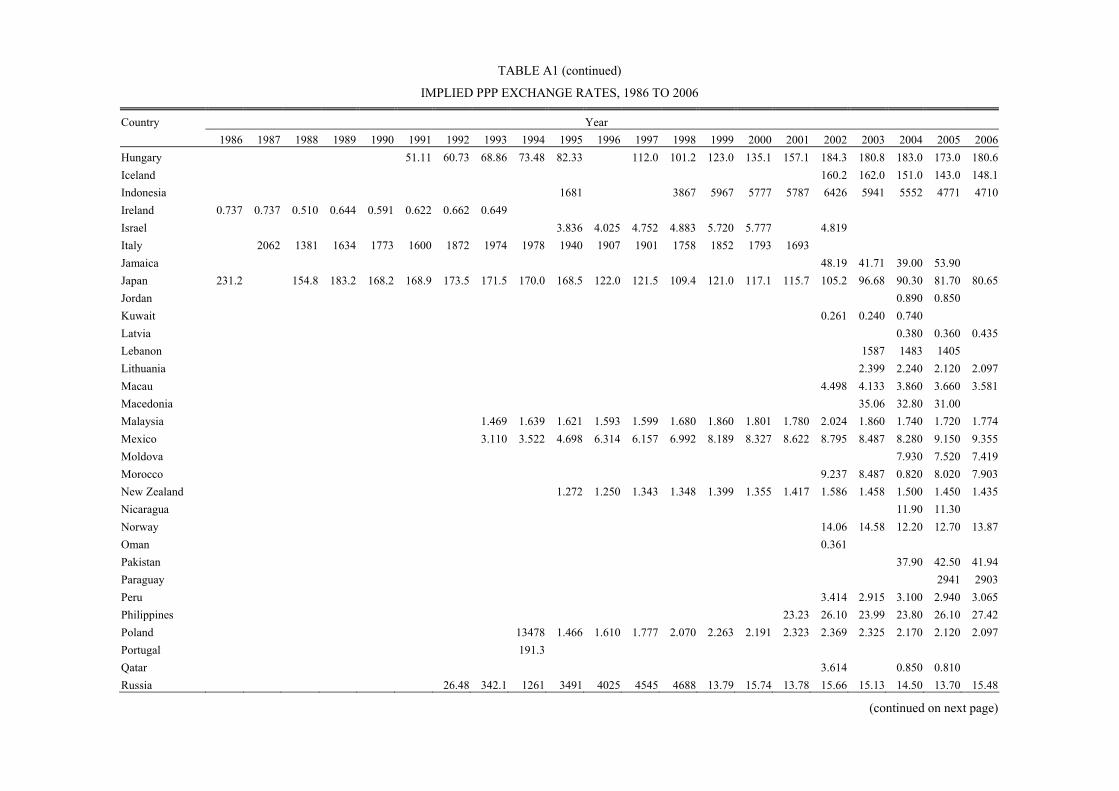
TABLE A1 (continued)

IMPLIED PPP EXCHANGE RATES, 1986 TO 2006

Country Year 1986 1987 1988 1989 1990 1991 1992 1993 1994 1995 1996 1997 1998 1999 2000 2001 2002 2003 2004 2005 2006 Hungary 51.11 60.73 68.86 73.48 82.33 112.0 101.2 123.0 135.1 157.1 184.3 180.8 183.0 173.0 180.6 Iceland 160.2 162.0 151.0 143.0 148.1 Indonesia 1681 3867 5967 5777 5787 6426 5941 5552 4771 4710 Ireland 0.737 0.737 0.510 0.644 0.591 0.622 0.662 0.649 Israel 3.836 4.025 4.752 4.883 5.720 5.777 4.819 Italy 2062 1381 1634 1773 1600 1872 1974 1978 1940 1907 1901 1758 1852 1793 1693 Jamaica 48.19 41.71 39.00 53.90 Japan 231.2 154.8 183.2 168.2 168.9 173.5 171.5 170.0 168.5 122.0 121.5 109.4 121.0 117.1 115.7 105.2 96.68 90.30 81.70 80.65 Jordan 0.890 0.850 Kuwait 0.261 0.240 0.740 Latvia 0.380 0.360 0.435 Lebanon 1587 1483 1405 Lithuania 2.399 2.240 2.120 2.097 Macau 4.498 4.133 3.860 3.660 3.581 Macedonia 35.06 32.80 31.00 Malaysia 1.469 1.639 1.621 1.593 1.599 1.680 1.860 1.801 1.780 2.024 1.860 1.740 1.720 1.774 Mexico 3.110 3.522 4.698 6.314 6.157 6.992 8.189 8.327 8.622 8.795 8.487 8.280 9.150 9.355 Moldova 7.930 7.520 7.419 Morocco 9.237 8.487 0.820 8.020 7.903 New Zealand 1.272 1.250 1.343 1.348 1.399 1.355 1.417 1.586 1.458 1.500 1.450 1.435 Nicaragua 11.90 11.30 Norway 14.06 14.58 12.20 12.70 13.87 Oman 0.361 Pakistan 37.90 42.50 41.94 Paraguay 2941 2903 Peru 3.414 2.915 3.100 2.940 3.065 Philippines 23.23 26.10 23.99 23.80 26.10 27.42 Poland 13478 1.466 1.610 1.777 2.070 2.263 2.191 2.323 2.369 2.325 2.170 2.120 2.097 Portugal 191.3 Qatar 3.614 0.850 0.810 Russia 26.48 342.1 1261 3491 4025 4545 4688 13.79 15.74 13.78 15.66 15.13 14.50 13.70 15.48

(continued on next page)

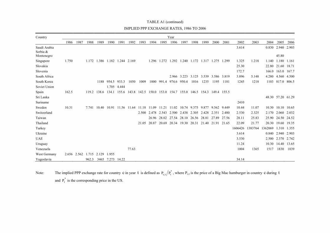
TABLE A1 (continued)

IMPLIED PPP EXCHANGE RATES, 1986 TO 2006

Country Year 1986 1987 1988 1989 1990 1991 1992 1993 1994 1995 1996 1997 1998 1999 2000 2001 2002 2003 2004 2005 2006 Saudi Arabia 3.614 0.830 2.940 2.903 Serbia & Montenegro 45.80 Singapore 1.750 1.172 1.386 1.182 1.244 2.169 1.296 1.272 1.292 1.240 1.172 1.317 1.275 1.299 1.325 1.218 1.140 1.180 1.161 Slovakia 25.30 22.80 21.60 18.71 Slovenia 172.7 166.0 163.0 167.7 South Africa 2.966 3.223 3.125 3.539 3.586 3.819 3.896 5.148 4.280 4.560 4.500 South Korea 1188 954.5 933.3 1050 1009 1000 991.4 974.6 950.4 1016 1235 1195 1181 1245 1218 1103 817.0 806.5 Soviet Union 1.705 4.444 Spain 162.5 119.2 138.6 134.1 155.6 143.8 142.5 150.0 153.0 154.7 155.0 146.5 154.3 149.4 155.5 Sri Lanka 48.30 57.20 61.29 Suriname 2410 Sweden 10.31 7.741 10.40 10.91 11.56 11.64 11.18 11.09 11.21 11.02 10.74 9.375 9.877 9.562 9.449 10.44 11.07 10.30 10.10 10.65 Switzerland 2.500 2.478 2.543 2.500 2.438 2.305 2.428 2.351 2.480 2.530 2.325 2.170 2.060 2.032 Taiwan 26.96 28.02 27.54 28.10 26.56 28.81 27.89 27.56 28.11 25.83 25.90 24.50 24.52 Thailand 21.05 20.87 20.69 20.34 19.30 20.31 21.40 21.91 21.65 22.09 21.77 20.30 19.60 19.35 Turkey 1606426 1383764 1362069 1.310 1.355 Ukraine 3.614 0.840 2.940 2.903 UAE 3.530 2.500 2.370 2.742 Uruguay 11.24 10.30 14.40 13.65 Venezuela 77.63 1004 1365 1517 1830 1839 West Germany 2.656 2.562 1.715 2.129 1.955 Yugoslavia 962.3 3465 7.273 14.22 34.14

Note: The implied PPP exchange rate for country c in year t is defined as *ttc, PP , where Pc,t is the price of a Big Mac hamburger in country c during t

and *tP is the corresponding price in the US.

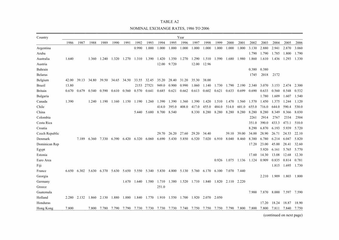
TABLE A2

NOMINAL EXCHANGE RATES, 1986 TO 2006

Country Year 1986 1987 1988 1989 1990 1991 1992 1993 1994 1995 1996 1997 1998 1999 2000 2001 2002 2003 2004 2005 2006 Argentina 0.990 1.000 1.000 1.000 1.000 1.000 1.000 1.000 1.000 1.000 3.130 2.880 2.941 2.870 3.060 Aruba 1.790 1.790 1.785 1.800 1.790 Australia 1.640 1.360 1.240 1.320 1.270 1.310 1.390 1.420 1.350 1.270 1.290 1.510 1.590 1.680 1.980 1.860 1.610 1.436 1.293 1.330 Austria 12.00 9.720 12.00 12.96 Bahrain 0.380 0.380 Belarus 1745 2018 2172 Belgium 42.00 39.13 34.80 39.50 34.65 34.50 33.55 32.45 35.20 28.40 31.20 35.30 38.00 Brazil 13.80 2153 27521 949.0 0.900 0.990 1.060 1.140 1.730 1.790 2.190 2.340 3.070 3.153 2.474 2.300 Britain 0.670 0.679 0.540 0.590 0.610 0.560 0.570 0.641 0.685 0.621 0.662 0.613 0.602 0.621 0.633 0.699 0.690 0.633 0.560 0.548 0.532 Bulgaria 1.780 1.609 1.607 1.540 Canada 1.390 1.240 1.190 1.160 1.150 1.190 1.260 1.390 1.390 1.360 1.390 1.420 1.510 1.470 1.560 1.570 1.450 1.375 1.244 1.120 Chile 414.0 395.0 408.0 417.0 455.0 484.0 514.0 601.0 655.0 716.0 644.0 590.4 530.0 China 5.440 5.680 8.700 8.540 8.330 8.280 8.280 8.280 8.280 8.280 8.280 8.349 8.366 8.030 Colombia 2261 2914 2767 2334 2504 Costa Rica 351.0 390.0 433.3 473.1 510.0 Croatia 8.290 6.870 6.193 5.939 5.720 Czech Republic 29.70 26.20 27.60 29.20 34.40 39.10 39.00 34.00 28.90 26.71 24.53 22.10 Denmark 7.189 6.360 7.330 6.390 6.420 6.320 6.060 6.690 5.430 5.850 6.520 7.020 6.910 8.040 8.460 8.380 6.780 6.214 6.047 5.820 Dominican Rep 17.20 23.00 45.00 28.41 32.60 Egypt 5.920 6.161 5.765 5.770 Estonia 17.60 14.30 13.08 12.68 12.30 Euro Area 0.926 1.075 1.136 1.124 0.909 0.835 0.814 0.781 Fiji 1.815 1.695 1.730 France 6.650 6.302 5.630 6.370 5.630 5.650 5.550 5.340 5.830 4.800 5.130 5.760 6.170 6.100 7.070 7.440 Georgia 2.210 1.909 1.803 1.800 Germany 1.670 1.640 1.580 1.710 1.380 1.520 1.710 1.840 1.820 2.110 2.220 Greece 251.0 Guatemala 7.900 7.870 8.000 7.597 7.590 Holland 2.280 2.132 1.860 2.130 1.880 1.880 1.840 1.770 1.910 1.550 1.700 1.920 2.070 2.050 Honduras 17.20 18.24 18.87 18.90 Hong Kong 7.800 7.800 7.780 7.790 7.790 7.730 7.730 7.730 7.730 7.740 7.750 7.750 7.750 7.790 7.800 7.800 7.800 7.811 7.840 7.750

(continued on next page)

TABLE A2 (continued)

NOMINAL EXCHANGE RATES, 1986 TO 2006

Country Year 1986 1987 1988 1989 1990 1991 1992 1993 1994 1995 1996 1997 1998 1999 2000 2001 2002 2003 2004 2005 2006 Hungary 75.12 79.70 88.18 103.0 121.0 178.0 213.0 237.0 279.0 303.0 272.0 224.0 210.3 203.5 206.0 Iceland 96.30 75.80 72.95 65.60 72.00 Indonesia 2231 8500 8725 7945 10855 9430 8740 9102 9542 9325 Ireland 0.740 0.698 0.620 0.710 0.630 0.620 0.610 0.649 Israel 2.950 3.170 3.380 3.700 4.040 4.050 4.790 Italy 1342 1229 1382 1230 1239 1233 1523 1641 1702 1551 1683 1818 1799 2088 2195 Jamaica 47.40 56.70 60.00 61.25 Japan 154.0 124.0 133.0 159.0 135.0 133.0 113.0 104.0 84.20 107.0 126.0 135.0 120.0 106.0 124.0 130.0 120.0 112.9 106.1 112.0 Jordan 0.706 0.714 Kuwait 0.310 0.300 0.292 Latvia 0.551 0.571 0.550 Lebanon 1512 1513 1511 Lithuania 3.150 2.872 2.789 2.690 Macau 8.030 8.030 8.042 7.957 7.990 Macedonia 55.80 51.25 50.00 Malaysia 2.580 2.690 2.490 2.490 2.500 3.720 3.800 3.800 3.800 3.800 3.800 3.783 3.822 3.630 Mexico 3.100 3.360 6.370 7.370 7.900 8.540 9.540 9.410 9.290 9.280 10.53 11.50 10.89 11.30 Moldova 11.84 12.53 13.20 Morocco 11.53 9.820 9.111 9.011 8.710 New Zealand 1.510 1.470 1.450 1.820 1.870 2.010 2.470 2.240 1.780 1.630 1.394 1.620 Nicaragua 15.87 16.38 Norway 8.560 7.160 6.816 6.414 6.100 Oman 0.390 Pakistan 57.42 59.86 60.10 Paraguay 6257 5505 Peru 3.430 3.460 3.483 3.267 3.260 Philippines 50.30 51.00 52.50 55.35 54.38 52.60 Poland 22433 2.340 2.640 3.100 3.460 3.980 4.300 4.030 4.040 3.890 3.875 3.312 3.100 Portugal 174.0 Qatar 3.640 3.696 3.682 Russia 98.95 686.0 1775 4985 4918 5739 5999 24.70 28.50 28.90 31.20 31.10 29.00 28.54 27.10

(continued on next page)

TABLE A2 (continued)

NOMINAL EXCHANGE RATES, 1986 TO 2006

Country Year 1986 1987 1988 1989 1990 1991 1992 1993 1994 1995 1996 1997 1998 1999 2000 2001 2002 2003 2004 2005 2006 Saudi Arabia 3.750 3.773 3.769 3.750 Serbia & Montenegro 67.35 Singapore 2.150 2.000 1.960 1.880 1.770 1.650 1.570 1.400 1.410 1.440 1.620 1.730 1.700 1.810 1.820 1.780 1.727 1.662 1.590 Slovakia 46.80 33.53 31.76 29.50 Slovenia 253.0 200.0 194.0 189.0 South Africa 4.260 4.430 5.040 6.220 6.720 8.130 10.90 7.560 6.688 6.609 6.600 South Korea 666.0 707.0 721.0 778.0 796.0 810.0 769.0 779.0 894.0 1474 1218 1108 1325 1304 1220 1173 1009 952.0 Soviet Union 0.600 1.740 Spain 133.0 111.0 117.0 106.0 103.0 102.0 114.0 138.0 124.0 126.0 144.0 156.0 155.0 179.0 189.0 Sri Lanka 98.57 100.4 103.0 Suriname 2179 Sweden 6.870 5.890 6.410 6.100 6.040 5.930 7.430 7.970 7.340 6.710 7.720 8.000 8.320 8.840 10.28 10.30 8.340 7.574 7.426 7.280 Switzerland 1.450 1.440 1.130 1.230 1.470 1.520 1.480 1.700 1.730 1.660 1.370 1.284 1.248 1.210 Taiwan 26.40 25.70 27.20 27.60 33.00 33.20 30.60 32.90 34.80 34.80 33.64 31.01 32.10 Thailand 25.16 25.30 24.60 25.30 26.10 40.00 37.60 38.00 45.50 43.30 42.70 40.60 40.83 38.40 Turkey 1324500 1600500 1530415 1.379 1.540 Ukraine 5.330 5.319 5.043 5.050 UAE 3.670 3.652 3.675 3.670 Uruguay 16.80 29.43 24.00 23.90 Venezuela 60.63 857.0 1598 2975 2614 2630 West Germany 2.020 1.887 1.660 1.890 1.680 Yugoslavia 1400 9001 11.72 15.12 67.80

Note: The nominal exchange rate is the domestic currency cost of one US dollar. An increase thus implies a depreciation of the domestic currency and vice

versa.

TABLE A3

REAL EXCHANGE RATES, 1986 TO 2006

Country Year 1986 1987 1988 1989 1990 1991 1992 1993 1994 1995 1996 1997 1998 1999 2000 2001 2002 2003 2004 2005 2006 Argentina 42.01 45.68 44.80 25.70 24.00 3.25 -2.37 2.84 -0.40 -1.59 -113.70 -64.38 -67.33 -61.62 -30.39 Aruba -64.43 -16.82 -23.57 -10.54 -11.42 Australia -40.51 -51.09 -17.63 -23.32 -15.39 -12.18 -25.74 -28.75 -24.56 -18.14 -22.21 -37.76 -37.71 -48.74 -51.66 -43.42 -37.46 -24.85 -19.85 -23.79 Austria 20.85 54.78 15.77 2.45 Bahrain -10.72 -19.19 Belarus -64.49 -80.30 -75.50 Belgium 29.21 36.29 7.89 12.04 24.10 25.33 38.52 38.75 29.74 50.34 39.23 24.37 11.38 Brazil -217.84 -21.58 20.47 -37.51 14.76 23.32 14.65 6.04 -35.42 -42.07 -43.51 -48.15 -60.35 -52.76 -24.85 -10.80 Britain 2.58 3.90 -8.12 5.56 4.23 28.17 33.21 20.27 13.89 18.86 13.57 19.81 17.66 23.02 17.90 11.36 14.74 14.86 14.84 11.33 16.26 Bulgaria -48.16 -44.63 -49.43 -46.79 Canada -16.27 -36.86 -11.16 -15.30 -9.63 5.74 -4.01 -11.14 -15.20 -11.53 -15.53 -26.46 -20.47 -25.82 -17.39 -16.04 -20.54 -22.31 -15.08 1.37 Chile -0.44 3.60 -1.35 17.32 7.06 6.09 -2.36 -19.19 -15.27 -32.64 -28.77 -18.63 -5.18 China -63.71 -42.11 -79.90 -78.91 -73.15 -76.13 -70.92 -74.16 -75.35 -67.48 -81.83 -84.40 -89.16 -86.32 Colombia 1.24 -24.19 -21.07 -9.43 -17.75 Costa Rica 0.12 6.69 -10.54 -24.85 -33.58 Croatia -32.60 -22.28 -18.63 -19.85 -16.73 Czech Republic -31.20 -19.53 -24.47 -28.76 -48.91 -59.06 -57.04 -40.83 -32.53 -31.47 -28.77 -14.86 Denmark 62.55 40.32 51.38 59.55 61.62 67.74 62.25 51.49 75.30 62.33 48.98 28.09 38.80 20.41 14.13 17.07 41.23 43.18 40.55 43.05 Dominican Rep 15.48 -3.81 -77.65 -37.11 -52.14 Egypt -69.58 -57.98 -67.33 -63.28 Estonia -43.03 -27.28 -24.85 -27.44 -25.66 Euro Area 11.33 -5.28 -11.61 -4.67 9.53 12.22 15.70 19.39 Fiji -21.07 -19.85 -14.27 France 43.27 54.56 25.13 31.89 35.70 34.78 39.82 41.84 32.18 50.76 36.84 22.75 10.25 -55.61 4.16 -2.13 Georgia -49.52 -41.55 -41.55 -29.61 Germany 13.49 22.55 24.45 15.67 40.50 31.19 16.90 4.96 11.27 -5.95 -10.04 Greece 7.14 Guatemala -20.66 -28.74 -37.11 -32.85 -31.04 Holland 17.60 27.70 8.71 17.00 23.85 21.60 28.34 30.05 21.56 41.58 30.63 15.95 2.81 8.99 Honduras -58.57 -38.57 -47.80 -48.84 Hong Kong -49.60 -89.73 -72.65 -68.95 -67.77 -64.30 -67.21 -65.88 -63.54 -61.25 -63.89 -66.53 -61.32 -65.07 -61.60 -55.05 -60.87 -63.49 -69.31 -69.42

(continued on next page)

TABLE A3 (continued)

REAL EXCHANGE RATES, 1986 TO 2006

Country Year 1986 1987 1988 1989 1990 1991 1992 1993 1994 1995 1996 1997 1998 1999 2000 2001 2002 2003 2004 2005 2006 Hungary -38.51 -27.18 -24.73 -33.77 -38.51 -46.34 -74.45 -65.55 -72.55 -65.69 -38.90 -21.42 -13.93 -16.25 -13.13 Iceland 50.92 75.95 72.75 77.93 72.10 Indonesia -28.30 -78.75 -37.99 -31.87 -62.89 -38.36 -38.60 -49.43 -69.31 -68.31 Ireland -0.34 5.49 -19.44 -9.82 -6.41 0.36 8.20 -0.04 Israel 26.27 23.89 34.07 27.74 34.78 35.51 0.61 Italy 43.01 11.64 16.73 36.55 25.57 41.76 25.92 18.69 13.07 20.65 12.17 -3.37 2.90 -15.24 -25.97 Jamaica 1.66 -30.70 -43.08 -12.78 Japan 40.65 22.19 32.01 5.61 22.40 26.59 41.71 49.14 69.39 13.15 -3.65 -21.05 0.82 9.99 -6.89 -21.15 -21.61 -22.31 -26.14 -32.84 Jordan 23.11 17.40 Kuwait -17.19 -22.38 92.82 Latvia -37.11 -46.20 -23.35 Lebanon 4.85 -2.02 -7.26 Lithuania -27.25 -24.85 -27.44 -24.91 Macau -57.96 -66.42 -73.40 -77.65 -80.26 Macedonia -46.48 -44.63 -47.80 Malaysia -56.30 -49.54 -42.94 -44.65 -44.68 -79.51 -71.44 -74.68 -75.87 -62.99 -71.45 -77.65 -79.85 -71.59 Mexico 0.31 4.70 -30.44 -15.47 -24.93 -20.00 -15.27 -12.23 -7.46 -5.37 -21.57 -32.85 -17.44 -18.89 Moldova -40.05 -51.08 -57.61 Morocco -22.17 -14.59 -240.79 -11.65 -9.72 New Zealand -17.19 -16.21 -7.67 -30.05 -29.01 -39.46 -55.54 -34.50 -19.98 -8.34 3.92 -12.09 Nicaragua -28.77 -37.11 Norway 49.60 71.08 58.22 68.31 82.15 Oman -7.60 Pakistan -41.55 -34.25 -35.99 Paraguay -75.50 -63.98 Peru -0.48 -17.14 -11.65 -10.54 -6.18 Philippines -77.26 -66.97 -78.34 -84.40 -73.40 -65.15 Poland -50.95 -46.79 -49.44 -55.66 -51.36 -56.44 -67.41 -55.10 -53.36 -51.48 -57.98 -44.63 -39.10 Portugal 9.48 Qatar -0.70 -146.97 -151.41 Russia -131.81 -69.58 -34.20 -35.61 -20.03 -23.32 -24.67 -58.31 -59.39 -74.07 -68.91 -72.06 -69.31 -73.40 -55.97

(continued on next page)

TABLE A3 (continued)

REAL EXCHANGE RATES, 1986 TO 2006

Country Year 1986 1987 1988 1989 1990 1991 1992 1993 1994 1995 1996 1997 1998 1999 2000 2001 2002 2003 2004 2005 2006 Saudi Arabia -3.68 -151.41 -24.85 -25.59 Serbia & Montenegro -38.57 Singapore -20.59 -53.48 -34.64 -46.42 -35.23 27.35 -19.21 -9.62 -8.71 -14.98 -32.38 -27.29 -28.78 -33.16 -31.72 -37.96 -41.55 -34.25 -31.42 Slovakia -61.50 -38.57 -38.57 -45.53 Slovenia -38.19 -18.63 -17.44 -11.93 South Africa -36.20 -31.80 -47.80 -56.39 -62.81 -75.56 -102.89 -38.43 -44.63 -37.11 -38.30 South Korea 57.88 30.02 25.81 30.00 23.69 21.07 25.40 22.40 6.12 -37.25 1.35 7.58 -11.50 -4.63 -0.19 -6.19 -21.07 -16.59 Soviet Union 104.41 93.78 Spain 20.03 7.17 16.95 23.51 41.23 34.37 22.35 8.34 21.03 20.50 7.33 -6.29 -0.44 -18.07 -19.50 Sri Lanka -71.33 -56.21 -51.91 Suriname 10.06 Sweden 40.62 27.32 48.36 58.13 64.88 67.48 40.90 33.01 42.32 49.58 33.05 15.86 17.15 7.85 -8.43 1.37 28.32 30.75 30.75 38.00 Switzerland 54.47 54.29 81.12 70.93 50.59 41.62 49.50 32.40 36.03 42.14 52.88 52.47 50.08 51.85 Taiwan 2.09 8.63 1.25 1.79 -21.70 -14.19 -9.28 -17.71 -21.34 -29.81 -26.14 -23.57 -26.95 Thailand -17.82 -19.25 -17.31 -21.83 -30.20 -67.76 -56.37 -55.05 -74.25 -67.31 -67.36 -69.31 -73.40 -68.51 Turkey 19.30 -14.55 -11.65 -5.13 -12.81 Ukraine -38.84 -184.57 -53.95 -55.36 UAE -3.89 -37.90 -43.87 -29.15 Uruguay -40.15 -104.98 -51.08 -56.05 Venezuela 24.71 15.83 -15.74 -67.33 -35.67 -35.77 West Germany 27.38 30.61 3.29 11.89 15.14 Yugoslavia -37.49 -95.45 -47.72 -6.12 -68.62

Notes: 1. The real exchange rate for country c in year t is defined as ( )*ct ct tctq log P S P= , where Pct is the price of a Big Mac hamburger in country

c during t , *tP is the corresponding price in the US and ctS is the nominal exchange rate, defined as the domestic currency cost of $US1. A positive

value of c,tq implies that the domestic currency is overvalued in real terms and vice versa. 2. All entries are to be divided by 100.

TABLE A4

PREDICTIVE REGRESSIONS WITH TIME DUMMIES, CHANGES IN NOMINAL EXCHANGE RATES, 24 COUNTRIES,1994-2006 h h

s, , h s, ,tc,t+h c,t s c,t s,ct- ) D-(s s = + d +uτ τ τ+ τ∑ α φ

(Standard errors in parentheses)

Horizon Year dummies s, , hτ τ+α ( 100)× hsη = Slope No of R2

h 94, 94+h 95, 95+h 96, 96+h 97, 97+h 98, 98+h 99, 99+h 00, 00+h 01, 01+h 02, 02+h 03, 03+h 04, 04+h 05, 05+h ( )hτ s,τ,τ+h1 N α∑ h

sφ Obs.

( )100× (1) (2) (3) (4) (5) (6) (7) (8) (9) (10) (11) (12) (13) (14) (15) (16) (17)

A. With overlapping observations

1 70.13 (15.73) 1.13 (16.30) -1.64 (16.05) -9.58 (15.63) 18.18 (15.42) -4.18 (15.36) -9.77 (15.49) -7.56 (15.76) 3.09 (15.70) 2.30 (15.52) 4.05 (15.50) 0.94 (15.41) 5.59 (4.43) -0.304 (0.301) 288 0.073 2 65.81 (18.00) -5.10 (18.71) -14.03 (18.40) 10.24 (17.87) 14.48 (17.61) -11.83 (17.53) -13.77 (17.70) -1.24 (18.04) 7.60 (17.96) 8.45 (17.73) 6.30 (17.70) - 6.08 (5.28) -0.314 (0.360) 264 0.062 3 59.31 (20.40) -17.78 (21.29) 5.58 (20.90) 6.52 (20.23) 6.89 (19.92) -15.74 (19.81) -7.28 (20.03) 3.45 (20.45) 13.90 (20.35) 10.82 (20.06) - - 6.57 (6.28) -0.307 (0.428) 240 0.046 4 48.60 (23.11) 4.85 (24.21) 4.42 (23.73) 0.44 (22.90) 2.16 (22.50) -9.59 (22.37) -3.79 (22.64) 7.78 (23.16) 14.48 (23.04) - - - 7.70 (7.52) -0.466 (0.508) 216 0.024 5 69.62 (24.92) 3.25 (26.39) -1.45 (25.75) -2.39 (24.63) 8.02 (24.10) -5.17 (23.92) 1.64 (24.28) 8.76 (24.99) - - - - 10.28 (8.74) -0.578 (0.613) 192 0.042 6 66.37 (26.65) -3.74 (28.39) -4.83 (27.64) 4.39 (26.31) 12.45 (25.68) 0.99 (25.47) 3.71 (25.90) - - - - - 11.33 (10.44) -0.613 (0.690) 168 0.040 7 58.66 (28.92) -7.80 (31.01) 1.49 (30.10) 8.92 (28.51) 18.71 (27.74) 3.32 (27.48) - - - - - - 13.88 (12.89) -0.606 (0.789) 144 0.033 8 56.17 (31.69) 0.91 (34.12) 8.05 (33.07) 16.36 (31.21) 20.39 (30.32) - - - - - - - 20.38 (16.11) -0.730 (0.891) 120 0.027 9 69.39 (33.12) 16.27 (36.19) 23.49 (34.87) 24.41 (32.51) - - - - - - - - 33.39 (20.98) -1.319 (1.027) 96 0.042 10 79.69 (35.36) 31.52 (39.06) 33.54 (37.48) - - - - - - - - - 48.25 (25.90) -1.813 (1.170) 72 0.061 11 94.53 (40.42) 47.50 (45.56) - - - - - - - - - - 71.02 (34.04) -2.560 (1.481) 48 0.091 12 119.20 (55.33) - - - - - - - - - - - 119.20 (55.33) -4.498 (2.674) 24 0.114

B. Without overlapping observations

1 70.13 (15.73) 1.13 (16.30) -1.64 (16.05) -9.58 (15.63) 18.18 (15.42) -4.18 (15.36) -9.77 (15.49) -7.56 (15.76) 3.09 (15.70) 2.30 (15.52) 4.05 (15.50) 0.94 (15.41) 5.59 (4.43) -0.304 (0.301) 288 0.073 2 68.69 (22.42) - -10.12 (23.19) - 13.21 (21.67) - -15.53 (21.84) - 4.86 (22.33) - 4.52 (21.85) - 10.94 (8.78) -0.564 (0.557) 144 0.067 3 72.12 (28.20) - - 17.35 (27.60) - - -15.11 (26.87) - - 2.39 (27.00) - - 19.19 (13.12) -1.418 (0.937) 96 0.057 4 52.87 (32.45) - - - 0.27 (30.78) - - - 10.42 (32.25) - - - 21.19 (17.59) -0.837 (0.992) 72 0.022 5 99.45 (38.59) - - - - -9.70 (33.25) - - - - - - 44.87 (24.88) -3.165 (1.718) 48 0.108 6 91.99 (37.63) - - - - - -11.94 (34.81) - - - - - 40.02 (23.61) -2.835 (1.565) 48 0.091 7 90.57 (56.80) - - - - - - - - - - - 90.57 (56.80) -3.373 (2.745) 24 0.064 8 96.85 (55.73) - - - - - - - - - - - 96.85 (55.73) -4.258 (2.694) 24 0.102 9 102.99 (54.60) - - - - - - - - - - - 102.99 (54.60) -4.233 (2.639) 24 0.105 10 108.26 (54.28) - - - - - - - - - - - 108.26 (54.28) -4.290 (2.624) 24 0.108 11 115.90 (54.98) - - - - - - - - - - - 115.90 (54.98) -4.413 (2.657) 24 0.111 12 119.20 (55.33) - - - - - - - - - - - 119.20 (55.33) -4.498 (2.674) 24 0.114

TABLE A5

PREDICTIVE REGRESSIONS WITH TIME DUMMIES, INFLATION DIFFERENTIALS, 24 COUNTRIES,1994-2006 h h

r, , h r, ,tc,t+h c,t r c,t r,ct-r Dr = + d +uτ τ τ+ τ∑ α φ

(Standard errors in parentheses)

Horizon Year dummies r, , hτ τ+α ( 100)× hrη = Slope No of R2

h 94, 94+h 95, 95+h 96, 96+h 97, 97+h 98, 98+h 99, 99+h 00, 00+h 01, 01+h 02, 02+h 03, 03+h 04, 04+h 05, 05+h ( )hτ r,τ,τ+h1 N α∑ h

rφ Obs.

( )100× (1) (2) (3) (4) (5) (6) (7) (8) (9) (10) (11) (12) (13) (14) (15) (16) (17)

A. With overlapping observations

1 -58.56 (15.57) 3.91 (16.13) 2.28 (15.88) -1.17 (15.46) -16.97 (15.26) -1.85 (15.19) 1.93 (15.33) 3.55 (15.59) -4.31 (15.53) -5.01 (15.35) -4.43 (15.33) 2.46 (15.24) -6.51 (4.38) -0.114 (0.297) 288 0.052 2 -53.28 (17.78) 9.87 (18.48) 4.68 (18.17) -14.65 (17.64) -20.14 (17.39) 0.37 (17.31) 4.73 (17.48) -3.09 (17.81) -11.74 (17.73) -10.90 (17.51) -3.59 (17.48) - -8.88 (5.22) -0.413 (0.355) 264 0.047 3 -49.59 (20.22) 12.66 (21.10) -7.36 (20.72) -13.59 (20.05) -18.82 (19.74) 4.79 (19.63) -0.29 (19.85) -10.55 (20.26) -18.39 (20.16) -10.03 (19.88) - - -11.12 (6.22) -0.691 (0.425) 240 0.044 4 -51.33 (22.74) -2.87 (23.82) -8.27 (23.35) -10.39 (22.53) -14.15 (22.14) 1.64 (22.02) -4.77 (22.28) -14.73 (22.79) -15.94 (22.67) - - - -13.42 (7.40) -0.738 (0.500) 216 0.037 5 -67.78 (24.96) -4.60 (26.43) -5.61 (25.79) -5.53 (24.67) -17.19 (24.14) -2.50 (23.96) -8.35 (24.32) -11.70 (25.03) - - - - -15.41 (8.76) -0.733 (0.614) 192 0.045 6 -68.73 (26.85) -0.76 (28.60) 0.25 (27.85) -8.01 (26.51) -21.64 (25.87) -6.22 (25.66) -5.80 (26.09) - - - - - -15.84 (10.52) -0.794 (0.695) 168 0.045 7 -66.05 (29.10) 4.05 (31.20) -2.90 (30.29) -12.20 (28.69) -25.23 (27.91) -3.24 (27.66) - - - - - - -17.60 (12.97) -0.788 (0.794) 144 0.038 8 -61.94 (31.98) -0.27 (34.43) -8.12 (33.37) -16.49 (31.50) -21.91 (30.60) - - - - - - - -21.74 (16.26) -0.720 (0.899) 120 0.026 9 -72.45 (33.68) -16.23 (36.79) -21.86 (35.45) -19.82 (33.06) - - - - - - - - -32.59 (21.34) -0.073 (1.044) 96 0.023

10 -81.81 (36.11) -28.11 (39.89) -25.97 (38.27) - - - - - - - - - -45.30 (26.45) 0.379 (1.195) 72 0.029 11 -93.12 (40.80) -37.32 (45.98) - - - - - - - - - - -65.22 (34.35) 1.046 (1.495) 48 0.041 12 -112.79 (55.25) - - - - - - - - - - - -112.79 (55.25) 3.009 (2.671) 24 0.055

B. Without overlapping observations

1 -58.56 (15.57) 3.91 (16.13) 2.28 (15.88) -1.17 (15.46) -16.97 (15.26) -1.85 (15.19) 1.93 (15.33) 3.55 (15.59) -4.31 (15.53) -5.01 (15.35) -4.43 (15.33) 2.46 (15.24) -6.51 (4.38) -0.114 (0.297) 288 0.052

2 -56.20 (22.11) - 0.72 (22.87) - -18.86 (21.37) - 6.51 (21.54) - -8.97 (22.02) - -1.78 (21.54) - -13.10 (8.65) -0.160 (0.549) 144 0.044 3 -62.48 (27.96) - - -24.49 (27.37) - - 7.59 (26.65) - - -1.55 (26.77) - - -20.23 (13.01) 0.427 (0.929) 96 0.038 4 -56.80 (31.86) - - - -11.74 (30.22) - - - -10.74 (31.67) - - - -26.43 (17.28) -0.264 (0.974) 72 0.029 5 -100.70 (38.79) - - - - 2.51 (33.42) - - - - - - -49.10 (25.01) 2.121 (1.727) 48 0.083 6 -98.86 (38.04) - - - - - 12.61 (35.19) - - - - - -43.12 (23.87) 1.819 (1.582) 48 0.082 7 -105.82 (56.56) - - - - - - - - - - - -105.82 (56.56) 2.660 (2.734) 24 0.041 8 -99.62 (56.78) - - - - - - - - - - - -99.62 (56.78) 2.548 (2.744) 24 0.038 9 -106.22 (55.87) - - - - - - - - - - - -106.22 (55.87) 2.855 (2.700) 24 0.048

10 -109.63 (55.68) - - - - - - - - - - - -109.63 (55.68) 2.791 (2.691) 24 0.047 11 -112.91 (55.57) - - - - - - - - - - - -112.91 (55.57) 2.762 (2.686) 24 0.046 12 -112.79 (55.25) - - - - - - - - - - - -112.79 (55.25) 3.009 (2.671) 24 0.055

TABLE A6

SEEMINGLY UNRELATED REGRESSIONS WITH TIME DUMMIES, 24 COUNTRIES, 1994-2006 h h

s, , h s, ,tc,t+h c,t s c,t s,ct- ) D-(s s = + d +uτ τ τ+ τ∑ α φ and h hr, , h r, ,tc,t+h c,t r c,t r,ct-r Dr = + d +uτ τ τ+ τ∑ α φ

(Standard errors in parentheses)

Horizon Year dummies s, , hτ τ+α ( 100)× hsη = Slope No of

h 94, 94+h 95, 95+h 96, 96+h 97, 97+h 98, 98+h 99, 99+h 00, 00+h 01, 01+h 02, 02+h 03, 03+h 04, 04+h 05, 05+h ( )hτ s,τ,τ+h1 N α∑ h

sφ Obs.

( )100× (1) (2) (3) (4) (5) (6) (7) (8) (9) (10) (11) (12) (13) (14) (15) (16)

A. With overlapping observations

1 62.16 (15.23) -2.34 (15.78) -2.08 (15.54) -2.17 (15.12) 17.35 (14.93) -0.03 (14.86) -4.37 (15.00) -4.80 (15.26) 3.93 (15.19) 4.17 (15.02) 4.31 (15.00) -1.40 (14.91) 6.23 (4.29) -0.705 (0.291) 288 2 55.49 (17.38) -9.03 (18.07) -6.33 (17.77) 13.87 (17.25) 19.14 (17.01) -2.39 (16.93) -6.32 (17.09) 2.33 (17.42) 11.01 (17.34) 10.47 (17.12) 4.06 (17.10) - 8.39 (5.10) -0.539 (0.347) 264 3 51.41 (19.76) -13.62 (20.61) 7.02 (20.24) 12.26 (19.59) 16.58 (19.29) -6.84 (19.18) -1.13 (19.39) 9.22 (19.80) 17.55 (19.70) 10.18 (19.43) - - 10.26 (6.08) -0.309 (0.415) 240 4 51.85 (22.21) 2.50 (23.27) 9.00 (22.81) 12.29 (22.01) 16.43 (21.63) -0.13 (21.51) 6.39 (21.76) 16.05 (22.27) 16.21 (22.14) - - - 14.51 (7.23) -0.223 (0.489) 216 5 68.85 (24.30) 3.82 (25.74) 1.51 (25.12) 0.93 (24.02) 11.86 (23.50) -1.96 (23.33) 4.45 (23.68) 9.99 (24.37) - - - - 12.43 (8.53) -0.448 (0.598) 192 6 66.64 (26.03) -3.23 (27.73) -4.31 (26.99) 4.80 (25.70) 13.49 (25.08) 1.58 (24.87) 3.95 (25.29) - - - - - 11.85 (10.20) -0.567 (0.674) 168 7 59.69 (28.22) -7.28 (30.26) 1.68 (29.38) 9.38 (27.82) 19.62 (27.07) 3.31 (26.82) - - - - - - 14.40 (12.58) -0.551 (0.770) 144 8 55.50 (30.91) 0.98 (33.27) 8.04 (32.25) 16.35 (30.44) 20.22 (29.57) - - - - - - - 20.22 (15.71) -0.783 (0.868) 120 9 66.33 (32.08) 16.32 (35.05) 25.11 (33.77) 28.99 (31.49) - - - - - - - - 34.19 (20.32) -1.709 (0.995) 96

10 76.21 (33.91) 37.13 (37.46) 45.97 (35.94) - - - - - - - - - 53.10 (24.84) -2.525 (1.122) 72 11 95.64 (39.07) 55.42 (44.03) - - - - - - - - - - 75.53 (32.90) -2.960 (1.432) 48 12 113.89 (52.91) - - - - - - - - - - - 113.89 (52.91) -4.093 (2.557) 24

B. Without overlapping observations

1 62.16 (15.23) -2.34 (15.78) -2.08 (15.54) -2.17 (15.12) 17.35 (14.93) -0.03 (14.86) -4.37 (15.00) -4.80 (15.26) 3.93 (15.19) 4.17 (15.02) 4.31 (15.00) -1.40 (14.91) 6.23 (4.29) -0.705 (0.291) 288 2 56.60 (21.59) - -1.02 (22.33) - 18.67 (20.87) - -6.80 (21.03) - 8.83 (21.51) - 1.87 (21.04) - 13.03 (8.45) -0.831 (0.536) 144 3 61.61 (27.23) - - 25.13 (26.66) - - -6.91 (25.95) - - 1.47 (26.08) - - 20.33 (12.67) -1.428 (0.905) 96 4 59.37 (30.87) - - - 19.26 (29.28) - - - 10.95 (30.68) - - - 29.86 (16.74) -0.671 (0.944) 72 5 99.21 (37.37) - - - - -11.09 (32.20) - - - - - - 44.06 (24.09) -3.174 (1.664) 48 6 85.78 (36.32) - - - - - -11.34 (33.60) - - - - - 37.22 (22.79) -2.849 (1.511) 48 7 108.59 (54.17) - - - - - - - - - - - 108.59 (54.17) -3.712 (2.618) 24 8 93.59 (52.98) - - - - - - - - - - - 93.59 (52.98) -5.090 (2.561) 24 9 91.38 (50.32) - - - - - - - - - - - 91.38 (50.32) -5.593 (2.432) 24

10 103.33 (49.80) - - - - - - - - - - - 103.33 (49.80) -6.085 (2.407) 24 11 120.15 (52.36) - - - - - - - - - - - 120.15 (52.36) -5.338 (2.531) 24 12 113.89 (52.91) - - - - - - - - - - - 113.89 (52.91) -4.093 (2.557) 24