The Best of Rules and Discretion: A Case for Nominal GDP Targeting in India

Pranjul Bhandari and Jeffrey Frankel

CID Working Paper No. 284 July 2014

Copyright 2014 Bhandari, Pranjul; Frankel, Jeffrey; and the President and Fellows of Harvard College

at Harvard University Center for International Development Working Papers

1

The Best of Rules and Discretion: A Case for Nominal GDP Targeting in India

Pranjul Bhandari and Jeffrey Frankel, Harvard Kennedy School

Updated Aug.6 2014

Abstract

The recent revival of interest in nominal GDP (NGDP) targeting has come in the context of large advanced economies. We argue that the case for NGDP targeting is even more appealing for mid-sized developing countries, because they tend to be more susceptible to supply shocks and terms of trade shocks. For India, in particular, one major exogenous supply shock is the monsoon rains. NGDP targeting splits the impact of supply shocks automatically between inflation and real GDP growth. In the case of inflation targeting (IT), by contrast, the full impact of an adverse supply shock or terms of trade shock is felt as a loss in real GDP alone. NGDP targeting arguably achieves the best of both worlds: it automatically accommodates supply shocks as most central banks with discretion would do anyway, while retaining the advantage of anchoring expectations as rules are designed to do. We outline a simple theoretical model and derive the conditions under which an NGDP targeting regime would dominate other regimes such as IT for achieving objectives of output and price stability. We go on to estimate for the case of India the main parameters needed to ascertain whether these conditions hold, most notably the slope of the aggregate supply curve. We find that under certain plausible conditions, nominal GDP targeting is indeed better placed than IT, especially in the face of the supply shocks that developing countries tend to experience.

JEL numbers: F41, E52

Keywords: central bank, developing, emerging markets, GDP, income, India, inflation, monetary policy, monsoon, nominal, shock, supply, target, terms of trade

2

The Best of Rules and Discretion: A Case for Nominal GDP Targeting in India

India’s central bank is contemplating a move from its current multi-indicator monetary policy approach, towards a simple credibility-enhancing nominal rule. As of 2014, it seems to favor a flexible inflation target, which it hopes will help lower inflation expectations that have been high and sticky since 20101.

In the paper we evaluate whether nominal GDP (NGDP) might be a good alternative for a monetary policy target for India, especially in the face of supply shocks that it faces and the varying macroeconomic situations that it experiences2. We outline a simple model to compare NGDP targeting with other nominal rules. We find that under certain simplifying assumptions and plausible conditions, NGDP targeting can indeed dominate Inflation targeting (IT).

Exhibit 1: Elevated inflation expectations in India

The paper is organized as follows. Section I discusses the origins and resurgence of NGDP targeting. The proposal has surfaced several times in the last few decades – though not always as a solution to the same probem -- suggesting its all-weather-friend characteristics. Section II highlights a simple theoretical model which compares alternative nominal monetary policy rules in terms of their ability to minimize a quadratic loss function that captures the objectives of price stability and output stability. We set out the conditions necessary for one regime to dominate the other. Section III discusses the

1 RBI (2014). Mohan and Kapur (2009) see drawbacks to inflation targeting for India. 2 Ranging from high growth and low inflation in 2003-2006 to high growth and high inflation in 2010-11 to low growth and high inflation in the 2011-2014 period.

0.0

2.0

4.0

6.0

8.0

10.0

12.0

14.0

16.0

18.0

Mar

-07

Jun-

07Se

p-07

Dec-

07M

ar-0

8Ju

n-08

Sep-

08De

c-08

Mar

-09

Jun-

09Se

p-09

Dec-

09M

ar-1

0Ju

n-10

Sep-

10De

c-10

Mar

-11

Jun-

11Se

p-11

Dec-

11M

ar-1

2Ju

n-12

Sep-

12De

c-12

Mar

-13

Jun-

13Se

p-13

Dec-

13M

ar-1

4

Current 3-month ahead

1 year ahead WPI Inflation

CPI Inflation

% yoy Household Inflation Expectations

Source: RBI; based on mean inflation rate reported by 4,000 households

3

evolution of monetary policy in India since independence in 1947 and the central bank’s desire to adopt a nominal rule. Section IV visits the different supply side shocks to which the country seems susceptible and the appropriateness of NGDP targeting to deal with them. Section V empirically tests the conditions outlined in section II to ascertain if indeed NGDP targeting would be appropriate in India in the sense of minimizing the quadratic loss function. We use two-stage-least-squares to estimate the parameters of the supply curve. Section VI addresses some practical concerns in implementing a NGDP rule. Operational complications arise from revisions in the nominal GDP statistics; but we find that inflation targeting has similar limitations. Section VIII concludes with thoughts on further research.

I. Origins and resurgence of NGDP targeting and relevance for developing countries:

The earliest proponents of nominal GDP targeting were Meade (1978) and Tobin (1980), followed by other economists in the 1980s. The historical context was a desire to earn credible monetary discipline and lower inflation rates. The early 1980s saw monetarism as the official policy regime in some major countries. It was soon frustrated, however by an unstable money demand function.

NGDP targeting had been designed specifically to counter such velocity shocks. Nevertheless it was not adopted. The concept was on the backburner for several decades. Instead, the dominant approach for many smaller and developing countries between the mid-1980s and mid-1990s was a return to exchange rate targets.

A series of speculative attacks in the late 1990s forced many countries to abandon exchange rate anchors and move to some form of floating exchange rates. Another reason mid-sized open countries may want to have a floating exchange rate is to accommodate terms of trade shocks and other real shocks. But if the exchange rate is not to be the anchor for monetary policy, what is? The 2000s saw the spread of IT from some advanced economies to many emerging market countries. Over the last two decades, it is believed to have contributed to bringing down inflation across many countries and to have anchored expectations.

The Global Financial Crisis (GFC) of 2008-09 provoked concerns over shortcomings of IT, analogous perhaps to the frustrations with exchange rate targets that had resulted from the currency crises of the 1990s. Criticisms of Inflation Targeting include its narrow focus, lack of attention to asset market bubbles, failure to hit announced targets, and mistaken tightening in response to supply shocks such as the mid-2008 oil price spike.

Meanwhile, interest in NGDP targeting revived, as an alternative to inflation targeting3. But it has been focused on advanced economies such as the US, UK, Japan and Euroland, where interest rates have been constrained by ‘zero lower bound’. The motive for NGDP targeting in this literature is to achieve a credible monetary expansion and higher inflation rates, which are quite the opposite of what Meade (1978) and Tobin (1980) had in mind. This flexibility of NGDP targeting, as a practical way to achieve the

3 E.g. Woodford’s (2012) theoretical analysis, Hatzius’ (2011) market viewpoint and Scott Sumner’s blog posts

4

goal of the day, be it monetary easing or tightening, and its focus on stabilizing demand are longstanding advantages.

Attention to developing and middle income countries in the NGDP targeting literature is scant4. And yet they may be the ones who can benefit the most from an NGDP target.

Developing countries have some characteristics that differ from advanced countries when it comes to setting monetary policy5. First, many developing countries have more acute need of monetary policy credibility. Some are newly born with an absence of well-established institutions, some have recently moved to a new monetary policy setting, some have a checkered past with central banks accommodating government debt, and some have had periods of hyperinflation.

The need for credibility amplifies the need to choose a nominal target which the central bank does not keep missing repeatedly. Central banks should choose targets ex ante that they will be willing to live with ex post and that they have relatively higher ability to achieve. For instance, announcing a strict inflation target that is then repeatedly missed would tend to erode credibility. One study showed that IT central banks in emerging market countries miss declared targets by much more than do industrialized countries (Fraga, Goldfajn and Minella, 2003).6

Second, developing and middle income countries tend to be more exposed to trade shocks (because they are more likely to export commodities and be price takers on world markets) and supply shocks (because of the importance of agriculture, social instability and productivity changes). Productivity shocks are likely to be larger in developing countries: during a boom, the country does not know in real time whether rapid growth is a permanent increase in productivity growth (it is the next Asian tiger) or temporary (the result of a transitory fluctuation in commodity markets or domestic demand).7

Weather disasters and terms of trade shocks are particularly useful from an econometric viewpoint, because these supply shocks are both exogenous and measureable. Exhibit 2 below shows that they tend to be bigger in emerging markets and low-income countries than in advanced economies.

The best choice of target variable depends on the type of shock to which the country is susceptible. If supply shocks are rife, NGDP targeting may be the right prescription. It splits the effects between inflation and GDP growth rather than suffering adverse supply shocks in the form of lost GDP alone.

Three categories of supply or trade shocks are relevant in particular:

a. Pure supply shock – Natural disasters (such as an earthquake, hurricane, cyclone, tidal wave, or flood), other weather-related events (drought or severe winter), social disruption (labor strike or

4 The few studies available include Frankel (1995b), McKibbin and Singh (2003), and Frankel, Smit and Sturzenegger (2008) for East Asia, India and South Africa respectively. 5 A thorough survey is available in Frankel (2011). 6 In part this may be because central banks in developing countries have a harder time hitting any target than in advanced economies: the monetary transmission mechanism usually works poorly due to oligopolistic banks and undeveloped financial markets. Mishra and Montiel (2012). For India: Aleem (2010) and Mohanty (2012). 7 The trend growth rate in emerging market countries is highly variable: Aguiar and Gopinath (2007).

5

0

2

4

6

8

10

12

14

16

18

20

Advanced Economies Emerging Markets Low-Income Countries

Terms of Trade Shock

Natural Disaster

Frequency of Shocks Across Country Groups(1970 - 2007)Probability (in %

of country years

social unrest), and other productivity shocks (technological progress) fall under this category. For India, a poor monsoon is a good example. A fixed exchange rate by definition prevents the currency from depreciating and thereby moderating the fall in the trade balance and GDP. A CPI target, if interpreted literally, implies that monetary policy must be tightened enough to choke off any increase in the price level, leading again to lower GDP growth. Only in case of NGDP targeting can the currency respond to an adverse supply or terms of trade shocks by depreciating, helping the trade balance and splitting the adverse impact of the shock between inflation and growth.

b. Rise in import price. One form of terms of trade shocks is an increase in the world price of importable goods. For India, oil prices are a good example. In the case of an exchange rate target, by definition the currency is prevented from depreciating, with adverse implications for the trade balance and GDP. In the case of CPI targeting, if interpreted literally, the currency must actually appreciate to prevent a rise in CPI inflation, with even worse implications for the trade balance and growth. In case of NGDP targeting, by contrast, the currency is not led to appreciate. Again the adverse shock is split between between inflation and GDP growth rather than growth alone.

c. Fall in export price. Many developing countries export commodities that undergo large price swings on world markets. In the case of exchange rate targeting the currency cannot adjust. In the case of CPI targeting, depreciation is also limited as it would boost inflation. Thus the trade balance worsens, as does GDP growth. For the nominal GDP target, the currency depreciates, helping the trade balance as well as GDP growth to improve and moderating the economic contraction. Exhibit 2: Emerging markets and low income countries are more susceptible to supply shocks

Source: IMF, 2011

6

Some theoretical models developed originally for advanced countries do not allow for comparing nominal rules in the face of exogenous balance of payments shocks. The advanced country models tend to assume that financing temporary trade deficits internationally is not a problem as international capital markets function well enough to smooth consumption in the face of external shocks. However, it is well documented by now that for developing countries, international capital markets can indeed exacerbate external shocks or even start them off. Capital inflow booms followed by sudden stops, sharp reversals, sharp depreciation and prolonged recessions are common in developing markets8.

NGDP targeting could potentially bring in the benefits of discretion without incurring the cost of inflation bias. In the model below, we formalize this intuition and probe further on when an NGDP target would dominate.

II. Theoretical underpinnings: Comparing discretion with four alternative nominal rules:

It is well established that a credible nominal target eliminates the inflationary bias that discretion otherwise allows in a Barro-Gordon (1983) type model of dynamic inconsistency. But it makes a difference what is the choice of nominal target, because the economy is vulnerable to short run shocks (Rogoff, 1985; Fischer, 1990). The impact of the shocks depends on the variable chosen to be the nominal target.

Using a simple model outlined by Frankel (1995a,b)9, we compare five alternative nominal policy rules in the conduct of monetary policy: full discretion by the central banker, rigid money supply rule, rigid exchange rate rule, rigid price level rule and rigid nominal GDP rule, respectively.

Our investigation of these policy rules is predicated on the argument that one wants to announce some simple variable to which the central bank will commit. Credible commitment to a nominal target, for example, is a means of defeating the inflation bias from Barro-Gordon dynamic inconsistency. The desire for transparency and accurate communication is not limited, however, to the Barro-Gordon argument for credible commitment to disinflation. It includes also the recent arguments for credible commitment to higher inflation. It is not even limited to a choice among alternative nominal anchors like M1 or inflation; the desire to offer forward guidance has included other intermediate targets such as the unemployment rate.10

The various Taylor rules are not members of this set of nominal-target commitments. One could view the Taylor rules as writing down what discretion would do. Or, as in "Flexible Inflation Targeting," one 8 E.g. Reinhart and Reinhart (2009); Reinhart and Rogoff (2011); Mendoza and Terrones (2012). 9 An inflation target for an open economy, which was not covered in Frankel (1995a,b), is also derived here. 10 The Federal Reserve and Bank of England attempted to carry forward guidance a step further in 2012-13 by declaring specific unemployment thresholds that were to be attained before interest rates would raised. These thresholds had to be abandoned in early 2014, however, arguably because of an unexpected fall in the labor force participation rate in the US and in productivity growth in the UK. A threshold expressed in terms of NGDP would have been more robust.

7

could view them as an intermediate (say monthly) means toward achieving a one-year or two-year target. Either way, Taylor rules do not compete directly with IT, NGDP, etc.

Our model includes the money supply, an important variable in our view in thinking about the question of sterilization and allowing authorities the possibility to affect exchange rates. This is another departure from some of the advanced country models that have done away with the money supply on the grounds that money demand is unstable and central banks tend to use interest rates as their main policy instruments.

Inflation targeting and NGDP targeting can be formulated in terms of either levels or rates of change. A possible advantage of targeting a level is a faster return to the goal. If the regime is credible, an incipient shortfall in the NGDP level during the course of the year engenders expectations of a coming monetary expansion and higher inflation, thus contributing to lower real interest rates and an accelerated move towards the goal.11 The disadvantage of targeting a level is that the public may not fully understand, comprehend or believe a target in levels as it would a target in growth rates. For our model, the distinction between levels and growth may not be important. Targets are set each year; announcing it in levels or growth would amount to the same thing.

While we show derivations for different nominal rules here, our primary question of interest is CPI inflation targeting versus NGDP targeting. The former is the rule the RBI is currently considering and the latter is the rule we focus on.

To simplify the analysis, we assume rigid rules in our theoretical analysis, keeping in mind that welfare ranking for rigid rules in theory might be different than that for flexible rules (Rogoff, 1985). We start with the closed economy model and then move on to an open economy set-up.

The aggregate supply relationship is assumed to be:

(1) y = ȳ + b(p – pe) + u,

where y is real output, ȳ is potential output, p is the price index, pe is the expected price index (all variables can be in log levels or annual growth rate), and u is a supply disturbance.

A. Closed economy objective function:

We assume objectives captured by the quadratic loss function:

(2) L = ap2 + (y – ŷ)2 ,

where a is the weight assigned to the inflation objective and ŷ is the desired level of output.

11 Indeed that is the very argument for targeting NGDP level for advanced economies constrained by a zero-lower-bound (Woodford, 2012).

8

In order to build an expansionary bias to discretionary policy making, the ŷ > ȳ condition is imposed, as in Barro and Gordon (1983). For simplicity we have assumed that the preferred level of inflation is zero. Substituting (1) into (2),

(3) L = ap2 + [ȳ - ŷ + b(p – pe) + u]2 .

(i) Discretionary policy:

Under full discretion, the policy maker chooses aggregate demand so as to minimize the loss function every period (i.e. dL/dp = 0) giving:

(4) p = [- b(ȳ - ŷ) + b2pe – bu] / [a + b2].

Under rational expectations,

(5) pe = Ep =(ŷ - ȳ)b/a.

This term reflects the inflationary bias that Barro and Gordon (1983) attribute to discretion. Central banks have to inflate just to keep up with expectations, even without achieving higher output. The aim of a credible nominal target is to remove this inflationary bias. However, the economy will still be vulnerable to short run shocks, the impact of which will depend on the variable it chooses as the nominal target (Rogoff, 1985; Fischer, 1990).

Combining (5) and (4) gives the solution for inflation under discretion:

(6) p = (ŷ - ȳ) [b/a] – ub/[a+b2].

Combining (6) and (2) gives the value of the expected loss function:

(7) EL = (1 + b2/a)(ȳ - ŷ)2 + [a/(a + b2)] var(u)

The first term represents the inflationary bias while the second represents the impact of supply disturbance after authorities have chosen the optimal split between inflation and output.

(ii) Money rule:

The money market equilibrium condition is given as –

(8) m = p + y – v,

where v represents velocity shocks. We assume that v is uncorrelated with u. If authorities pre-commit to a money growth rule to reduce expected inflation in the long run equilibrium, they must give up on affecting y. The optimal money growth rate is the one that sets Ep = 0; thus setting money supply, m, at Ey, which in this case is ȳ. The aggregate demand equation thus becomes:

(9) p + y = ȳ + v.

9

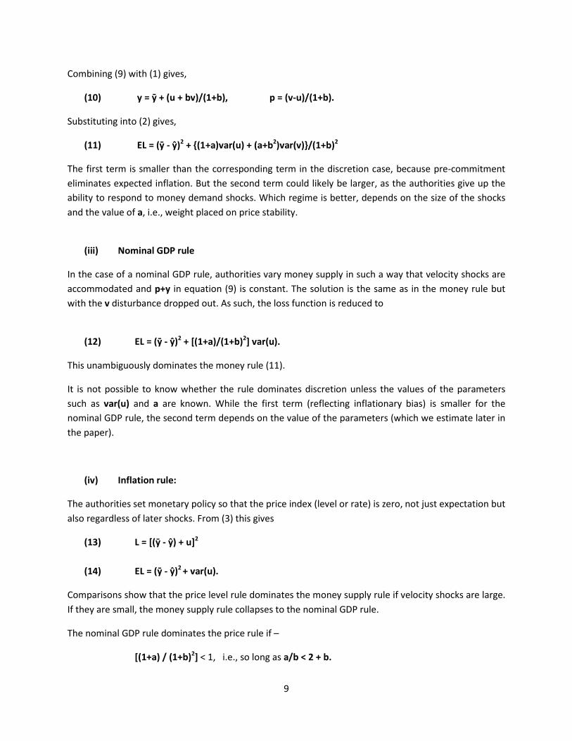
Combining (9) with (1) gives,

(10) y = ȳ + (u + bv)/(1+b), p = (v-u)/(1+b).

Substituting into (2) gives,

(11) EL = (ȳ - ŷ)2 + {(1+a)var(u) + (a+b2)var(v)}/(1+b)2

The first term is smaller than the corresponding term in the discretion case, because pre-commitment eliminates expected inflation. But the second term could likely be larger, as the authorities give up the ability to respond to money demand shocks. Which regime is better, depends on the size of the shocks and the value of a, i.e., weight placed on price stability.

(iii) Nominal GDP rule

In the case of a nominal GDP rule, authorities vary money supply in such a way that velocity shocks are accommodated and p+y in equation (9) is constant. The solution is the same as in the money rule but with the v disturbance dropped out. As such, the loss function is reduced to

(12) EL = (ȳ - ŷ)2 + [(1+a)/(1+b)2] var(u).

This unambiguously dominates the money rule (11).

It is not possible to know whether the rule dominates discretion unless the values of the parameters such as var(u) and a are known. While the first term (reflecting inflationary bias) is smaller for the nominal GDP rule, the second term depends on the value of the parameters (which we estimate later in the paper).

(iv) Inflation rule:

The authorities set monetary policy so that the price index (level or rate) is zero, not just expectation but also regardless of later shocks. From (3) this gives

(13) L = [(ȳ - ŷ) + u]2

(14) EL = (ȳ - ŷ)2 + var(u).

Comparisons show that the price level rule dominates the money supply rule if velocity shocks are large. If they are small, the money supply rule collapses to the nominal GDP rule.

The nominal GDP rule dominates the price rule if –

[(1+a) / (1+b)2] < 1, i.e., so long as a/b < 2 + b.

10

The conclusion is NGDP targeting dominates IT except in the presence of a very steep supply curve and/or a very high weight on the price stability objective in the quadratic loss function.

The condition can be simplified further if one is willing to infer an estimate a, the weight on price stability, from the Taylor Rule. The original Taylor Rule, which is still widely used, gives equal weights to output and price stability in setting its real interest rate policy instrument, implying a = 1. Then the condition a/b < 2 + b collapses to b > √𝟐 – 1. This implies that for the nominal GDP rule to dominate the price rule, the AS curve must be flat enough that its slope (1/b) is less than 2.414.

B. Open economy objective function:

The conduct of monetary policy in an open economy accounts for the exchange rate. To account for the central bank’s objective of having a stable exchange rate, we include it directly in the loss function along with output and inflation.12 The intention is to err on the side of exchange rate targeting and to understate the case for NGP targeting.

The open economy loss function (equivalent to equation 2 from above) now looks as follows:

(15) L = ap2 + (y – ŷ)2 + cs2 ,

Where s is the spot rate measured relative to some equilibrium or target value and c is the weight placed on exchange rate stability. We assume here that the central bank would like to minimize volatility in the exchange rate around its average value.

Rather than specifying a full-fledged model for a free floating exchange rate, we attribute the bulk of the variation to an error term that we call e here. This is in line with the fact that much of the variation in exchange rate (even ex post) is hard to explain. We also include the money supply, to allow authorities the possibility of affecting the exchange rate. (If the exchange rate is fixed, then e can be interpreted as a balance of payments shock, which shows up in the money supply.) Our equation is as follows:

(16) s = m – y + e .

We assume that e is uncorrelated with the supply disturbance u.

We have specified above that m = p + y – v. Combining equations (8) and (16) gives:

(17) s = p – v + e .

Combining with the aggregate supply equation (1), we can write the loss function (15) as:

(18) L = ap2 + [ȳ - ŷ + b (p - pe) + u]2 + c(p – v + e)2 .

12 The exchange rate could also have been included indirectly via the consumer price index or the trade balance, but here we choose to deal with it directly.

11

We consider the alternative nominal rules below.

(i) Discretionary policy

As in the closed economy case, authorities can set dL/dp = 0. This gives:

(19) p = [-(ȳ - ŷ)b + b2pe – bu + c(v-e)] / [a+b2+c].

Rationally expected p is given by pe = Ep:

(20) pe = [-b(ȳ - ŷ)] / (a+c).

Similar to the closed economy case, this term reflects the inflationary bias that Barro and Gordon (1983) attribute to discretion.

Combining (19) and (20) gives:

(21) p = - (ȳ - ŷ) [b/(a+c)] + [c(v-e) – bu] / [a+b2+c] .

The loss function works out as:

(22) EL = [ȳ - ŷ]2 (a+b2+c) / (a+c) + {(a+c) var(u) + c(a + b2) [var(v) + var(e)]} / (a+b2+c) .

(ii) Money rule

As in the closed economy case, expected inflation is zero and the authorities set m at ȳ, giving the condition p + y = ȳ + v as shown above. This gives the solutions for y and p as outlined in (10). Combining the solution of p with (17) gives the value for s:

(23) s = e – [(u+bv) / (1+b)] .

The values for p, y and s are now inserted in the open economy loss function to give:

(24) EL = [ȳ - ŷ]2 + [(1+a+c) / (1+b2)] var(u) + [(a + b2 + cb2) / (1 + b)2] var(v) + [c] var(e) .

The comparison with discretion, as in the closed economy case, depends on the various magnitudes.

(iii) Nominal GDP rule

As in the closed economy case, the monetary authorities are able to vary m so as to keep p+y constant. The velocity shocks, v, therefore drop out and the expected loss function becomes:

(25) EL = [ȳ - ŷ]2 + [(1+a+c) / (1+b2)] var(u) + [c] var(e).

12

As before, this unambiguously dominates the money rule.

(iv) Exchange rate rule

The authorities peg the exchange rate in such a way that Ep = 0, because (17) then implies that s = 0. The ex post price level is given by:

(26) p = v – e.

From (1), it follows that

(27) y = ȳ + b(v – e) + u .

From (14), it follows that:

(28) EL = (a+b2) var(v-e) + [ȳ - ŷ]2 + var(u).

Assume that v and e are uncorrelated, so that var(v – e) can be replaced with var(v) + var(e)13. The coefficient on var(e) is (a+b2), which is likely to be larger than c, the coefficient on var(e) in the nominal GDP targeting rule (25)14. Arguing that e shocks tend to be larger than u shocks15, and v shocks lie somewhere between e and u shocks in magnitude, it can be inferred that the expected loss from fixing the exchange rate is greater than the expected loss from fixing nominal GDP.

(v) Inflation rule

With the inflation variable set to zero, it can be inferred from (18) that the expected loss will be:

(29) L = [(ȳ - ŷ) + u]2 + c(-v + e]2 and

(30) EL = [ȳ - ŷ]2 + var(u) + c var(e) + c var(v) .

Comparing (30) with (28) shows that the price rule dominates the exchange rate rule if c < a + b2. This is easily met if c < a, meaning just that central bankers perceive price level fluctuations as more damaging than similar-magnitude exchange rate fluctuations.

From (25), it can be inferred that the nominal GDP rule dominates the price rule if the following condition holds:

a + c < b2.

13 This assumption is relaxed in Frankel (1995a, b). We have not considered this relaxation in this paper because it primarily affects the comparison of exchange rate targeting and NGDP targeting, which is not our main concern here. 14 Even in the very conservative case of a=c, a+b2 > c. 15 It is common for the exchange rate to move 10% or more a year, but similar movements in other macro variables are relatively rare.

13

(Velocity shocks add further to the relative superiority of NGDP targeting.) If c is indeed less than a, then a sufficient condition is a < b2/2 and the answer again depends on the magnitude of b relative to a. If we take a=1 from the Taylor Rule, the condition becomes simply b > √2 . Again, a very steep supply curve and/or a very high weight on the price stability objective could result in IT dominating NGDP targeting. To ascertain whether NGDP targets dominate inflation targets, we will need to estimate b.

We re-cap the key conditions, which depend on magnitudes of parameters that will be revisited in a later section:

Closed economy condition: For nominal GDP targeting to dominate price or inflation targeting, the condition is a < (2 + b)b. For a = 1, as in the original Taylor rule, this inequality boils down to a flat AS curve: 1/b < 2.414.

Open economy condition: For nominal GDP targeting to dominate price targeting, the condition is a + c < b2. For c < a and a = 1, the inequality is 1/b < 1/√2 = .707.

Having discussed the theoretical underpinnings, we will need some parameter estimates to ascertain whether the condition for NGDP targeting dominating IT is likely to hold for the case of India. We first discuss the evolution of monetary policy making in India before evaluating its suitability to a NGDP target.

III. Evolution of Monetary Policy making in India

A Brief history

India’s monetary policy framework has undergone several significant transformations. Starting with an exchange rate anchor after independence in 1947, it moved to the use of credit aggregates as the nominal anchor in 1957. Changes in the Bank rate and Cash Reserve Ratio were the main policy instruments supporting its credit allocation functions and ‘social control’ over channeling credit to ‘priority sectors’ (RBI, 2014).

Monetization of fiscal deficit, its inflationary consequence and crowding out of private sector credit called for a change in the monetary regime, leading to a new era of monetary targeting in 1985. Broad money was the intermediate target and reserve money was the main operating instrument. However this policy framework was also fraught with problems. Unconstrained credit to the government fuelled inflation. Capital flows (following the 1991 liberalization) further eroded control over monetary aggregates. Meanwhile, structural reforms in the 1990s led to a shift in financing patterns for the government. Gradually, interest rates and exchange rate started to become more market determined and the RBI was able to move from direct to more indirect market based instruments.

14

In 1998, the RBI moved to a ‘multiple indicators approach’, whereby it considered many variables – growth, inflation, exchange rates, credit growth, capital flows, fiscal position, trade, etc. This approach worked well for the next decade, with inflation rate (WPI and CPI-IW) falling from 8-9% to 5-6% over the ten years.16

Call for a new approach

However, the period 2010 - 2013 raised questions on the efficacy of the multiple indicators approach. Inflation was high and sticky and growth had fallen substantially for an extended period of time. Several commentators questioned the effectiveness of the approach, calling for a well-defined nominal target which would provide clarity with respect to what the RBI should do.

The RBI governor set up a committee of experts to recommend the way forward. The committee in its January 2014 report recommended a “flexible inflation target” for the conduct of monetary policy with the nominal anchor, the combined CPI inflation, set at 4% with a +/- 2% band17.

Exhibit 3 and 4: Inflation has been high and sticky and growth slowing in the 2010 to 2013 period

Source: CEIC

The report noted that India has one of the highest inflation rates amongst G-20 countries and that elevated inflation was creating macroeconomic vulnerabilities. (High inflation distinguishes those countries that were most hit by the rise in US interest rates in the “taper tantrum” of May-June 2013.18) The report emphasized that “high inflation itself becomes a risk to growth” and “limits the space for

16 E.g., Mohan (2009). 17 It also laid out a transition path: “The transition path to the target zone should be graduated to bringing down inflation from the current level of 10 per cent to 8 per cent over a period not exceeding the next 12 months and to 6 per cent over a period not exceeding the next 24 month period before formally adopting the recommended target of 4 percent inflation with a band of +/- 2 per cent”. 18 Klemm, Meier and Sosa (2014).

0.0

2.0

4.0

6.0

8.0

10.0

12.0

14.0GDP at Market Price

GDP at Factor Cost

India's GDP Growth% chg yoy

4

6

8

10

12

14

16

CPI Inflation Measures

CPI Industrial Workers

CPI Combined

% chg yoy

Long term average

15

accommodating growth concerns”19 implying that the current situation of stagflation would benefit from enhanced price stability.

It stated that –

“Stabilizing and anchoring inflation expectations – whether they are rational or adaptive – is critical for ensuring price stability on an enduring basis, so that monetary policy re-establishes credibility visibly and transparently, that deviations from desirable levels of inflation on a persistent basis will not be tolerated.”

IV. Vulnerability to supply shocks

Before moving on to discuss the suitability of NGDP targeting for India, we discuss the supply shocks to which the country is prone. In the January 2014 RBI report (referred to in the previous section), the central bank explicitly acknowledged “the vulnerability of the Indian economy to supply/external shocks …” and its impact on monetary policy. As argued in sections above, nominal GDP targeting is likely to dominate alternative rules when a country is vulnerable to supply shocks. Furthermore, we need exogenous and measureable supply shocks if we are to identify movements along the aggregate demand curve. (The productivity shocks so beloved of advanced-country macro models probably will not meet these criteria.)

India imports much of the oil and gas it consumes. It has recently also begun to import coal for fuelling its electricity plants. Thus it is susceptible to changes in global prices of fossil fuels. The World Bank’s index for the net barter terms of trade shows India as typical of emerging markets in the volatility of its terms of trade (exhibit 5).

India over the last few decades has faced natural disasters ranging from earthquakes and tsunamis, to super-cyclones and floods, often causing huge disruptions. It also suffers chronically from annual uncertainty regarding rains during the monsoon season. Data show that these rains have an important bearing on inflation and growth nationally, and not merely regionally. No doubt productivity shocks are also important in India as well, but they are neither as easily measured nor as clearly exogenous as weather events and terms of trade shocks.

The estimated aggregate demand relationship will incorporate whatever reaction function the monetary authorities follow during the sample period. If they target m, we are estimating equation (8). If they target inflation, then the weather and oil shocks should in theory show no effect on the price index. If they are already targeting nominal GDP, even if only implicitly, then the weather and oil shocks should have equiproportionate effects on output (negative) and the price level (positive).

19 Referring to Friedman (1977), Fischer (1993) and Barro (1995) .

16

Exhibit 5: India experiences terms-of-trade shocks like other Emerging Market countries

Source: World Bank, WDI

Exhibit 6 and 7: Association between monsoon rains and inflation/GDP growth

-25

-20

-15

-10

-5

0

5

10

15

0

2

4

6

8

10

12

Real GDP Growth Monsoon rains (RHS)% chg yoy% departure from normal

Monsoon Rains and Real GDP Growth

17

Source: CEIC

V. Estimating India’s aggregate supply curve

To undertake an evaluation of NGDP targeting versus inflation targeting, one must know a few key parameters, partially the slope of the AS curve (see section II.A.4). In principle, these parameters can be estimated, so long as we have good instrumental variables to identify the two equations. Our structure of equations for deriving these estimates is related to seminal work on estimating the New Keynesian Philips Curve (Roberts, 1995). The system of equations can be estimated in a 2SLS framework, i.e., using Instrumental Variables.

In one version of the equations, possible exogenous instruments to identify shifts in the Aggregate Supply curve include natural disasters such as droughts, hurricanes and earthquakes20 and increases in world prices of import commodities. Possible exogenous instruments to identify shifts in the Aggregate Demand curve include fluctuations in the incomes of major trading partners and military spending21.

For India, the supply shocks we used were fluctuations in terms of trade and the weather. The demand shocks we used were income among trading partners and shocks due to specific government-related spending. Each of them is described below.

We also tried a different method, the “triangle model” for estimating the Philips curve (Gordon, 2013), which emphasizes the role of inertia, uses the output gap/unemployment rate as the demand side indicator, and includes supply shock variables explicitly in the OLS equation. However, the productivity

20 Cavallo and Noy (2011).. 21 See Frankel (2013).

-30-25-20-15-10-5051015-8

-6

-4

-2

0

2

4

6

8

Misery Index Monsoon rains (RHS, inverted)ppts% departure from normal

Monsoon Rains and Misery Index (MI),MI = CPI Inflation rate - Real GDP growth rate

18

term shows up with the wrong sign, suggesting perhaps the problem of endogeneity in output. Instruments on the demand side may indeed be necessary.

Variables and data sources:

The data in the model span the 70 quarters from June 1996 (when India’s quarterly GDP data series started) to December 2013. As we are using quarterly data, the series are seasonally adjusted using the X-12 method.

Two measures for inflation are used – the Wholesale Price Index and the GDP deflator22. The WPI has been the most widely used measure of inflation in India over many years. It also feeds into the estimation of GDP accounts thereby correlating well with the GDP deflator. We do not include the new combined-CPI measure because for one thing with about three years-worth of data, it has an insufficient history23.

For the supply curve model, we use the actual annual inflation rate minus the expected annual inflation rate. The latter is calculated using a simple ARMA (1 1) model. Both WPI and GDP deflation annual inflation rates were checked for stationarity using the Augmented Dickey Fuller test. The Akaike Information criteria (AIC) and Bayesian Information Criteria (BIC) were used to choose the lag structure. The two dependent variables of actual inflation minus expected inflation are labelled WINARM and GINARM respectively. We also tried a random walk version where expected inflation is the previous period’s inflation rate. These are referred to as WINRW and GINRW respectively.

The output gap (OGAP) is calculated using real GDP at market prices for actual output, and a Hodrick-Prescott filtered series of real GDP at market price for potential output. The smoothing parameter of the HP filter is set at 1600 as is typical in quarterly data. The output gap is actual minus potential output, expressed as a percentage of potential output.

Central to our estimates are the exogenous instruments for demand and supply. For demand shocks we use world growth (WG) as an indicator of global demand for exports of goods and services.

We also try a domestic policy shock variable centered on the National Rural Employment Guarantee scheme (NREG). This social security scheme began in February 2006 as a flagship social security program of the then ruling United Progressive Alliance (UPA) government. This scheme guaranteed a minimum daily wage and employment to all rural Indians for hundred days a year. The multiplier effect of this program was far more than the actual fiscal expenditure incurred by the government. Several studies24 have documented that this social security scheme gave a new wave of bargaining power to rural Indians

22Derived from the series for GDP at market prices. 23Also, the CPI includes import prices, but supply decisions are made by domestic producers. If we think import prices enter the objective function and should be accounted for, our "open economy" version of the objective function applies (Section II.B). But P should refer to domestically determined prices. As such, WPI and GDP deflators are probably the right inflation indicators to use. 24 See Mann, Pande and Shah, 2012.

19

and was an important factor in increasing their prosperity which fed into inflation (through routes such as demand for more expensive protein-rich food items). Because the program did not originate as a response to lower growth, but rather had its roots in the political ideology of the ruling party, we find it exogenous and apt as a domestic policy shock variable. For our analysis, we use a dummy variable which takes the value zero before February 2006 and the value of the ratio of districts where it was rolled out after February 2006. So for instance it takes the value of 0.33 in the period the policy was launched in a third of India’s districts, moving to 0.5 when half the country was covered and finally 1.0 when it was universally rolled out.

For supply shock instruments, we use an international terms-of-trade indicator and a domestic weather-related indicator. The international terms of trade indicator is based on the US$ price of oil converted to Rupees using the spot USDINR exchange rate. The value of oil per bbl in (per 100) Rupees is then deflated by WPI inflation to get the real price of oil. The actual indicator used (OIL) is the quarter-over quarter change in the real price of oil. A 2-quarters lag worked best, attributable to fixed-price advance contracts on oil imports, which take time to renegotiate. This indicator reflects the vulnerability of India to oil imports.

The second supply shock is based on the monsoon rains (RAINS) in India between June and September every year. This is the main rainfall season and is key in determining the main Kharif (Summer) crop of the country. It also replenishes the water tables and is also associated with a good Rabi (Winter crop). Thus its impact on agricultural output and spillover into the rest of the economy lasts through the year. For our model, we use the monsoon rains’ percentage departure from normal series across four successive quarters. For instance if the percentage departure for monsoon rains is 2.3% from normal in 2003, we label the quarters ending June ’03, September ’03, Dec ’03 and Mar ’04 (when the winter crop is finally harvested), as 2.3%.

All GDP and WPI data are taken from the national Central Statistical Office (CSO) and the CEIC database. World growth is taken from IMF’s WEO. Oil price and exchange rate are taken from the CEIC database and monsoon deviation from normal data from the Indian Meteorological Department.

We try to keep the model as parsimonious as possible, given that there are only 70 observations (due to a short series for quarterly GDP in India). We are aware that our regressions may suffer from low statistical power and we will discuss this issue where appropriate.

Estimation results:

We report our main regressions in table 1 below. The upper half of the table shows the results from the first stage, and the second half shows the result from the second stage of the 2SLS framework. Regression 1 has the right sign for all variables. In the first stage regression, the demand shock variables - higher world growth and the NREGA scheme - have a positive effect on the output gap. In the second stage, the inverted aggregate supply curve, an increase in the oil price variable has a positive impact on inflation, while higher rains (implying a good crop) lower inflation.

20

Table 1: Estimation of Supply Relationship First Stage Dependent Variable: output gap Second Stage (Inverted supply equation) Dependent Variable: inflation surprises (winarm/ginarm/ginrw)

Note: First stage non-instrument variables have not been shown in the table. Memo: List of variables with brief description WINGAP and GINGAP: Annual actual minus expected inflation rate derived from an ARMA model for WPI inflation and GDP deflator respectively GINRW: Annual inflation rate minus expected inflation rate derived from a random walk assumption OGAP: Output gap based on GDP data with potential calculated by passing through the HP filter Aggregate demand instruments: WG: World annual GDP growth NREG: Dummy variable =0 when the program had not started and takes the value of ratio of districts covered when it was operating Aggregate supply shocks: OIL (-2): This terms of trade variable is calculated as US$ price of a barrel of oil x USDINR exchange rate, to get the Rupee value of oil; then deflated by WPI inflation index to convert to real terms. Quarterly change in the real value of oil. A two quarter lag worked best.

1 2 3 4VARIABLES ogap ogap ogap ogapFirst-stage regressionswg 0.541*** 0.495*** 0.558*** 0.561***

(0.109) (0.107) (0.109) (0.109)nreg 0.006a 0.006* 0.007*

(0.004) (0.004) (0.004)constant -0.019*** -0.015*** -0.020*** -0.020***

(0.005) (0.004) (0.004) (0.005)

R-squared 0.396 0.371 0.422 0.416Prob > F 0.000 0.000 0.000 0.000

VARIABLES winarm winarm ginarm ginrwSecond-stage regressionsogap 0.666*** 0.562*** 0.384** 0.533**

(0.203) (0.202) (0.182) (0.265)oil (-2) 0.093* 0.096* 0.074b 0.138*

(0.053) (0.05) (0.049) (0.071)rains -0.065** -0.057** -0.041* -0.081**

(0.026) (0.025) (0.024) (0.034)constant -0.003 -0.002 -0.002 -0.003

(0.002) (0.002) (0.002) (0.003)

Observations 70 70 65 66Standard errors in parentheses

*** p<0.01, ** p<0.05, * p<0.1ap=0.11, bp=0.135

21

RAINS: Percentage deviation of monsoon rains from normal. The data-point for each year’s monsoon rain (e.g. 2003) are applied for four consecutive quarters (ending June ’03, Sep ’03, Dec ’03 and Mar ’04)

Except for NREG, the others are significant in the 5 -10% level of significance. While at p=11%, NREG is not too far off from the accepted significance mark, we run regression 2 without the NREG variable. All main variables in Regression 2 are right signed and significant. The estimated slope of the supply curve is 0.56. Although we will discuss the range of estimates for important variables, regression 2 is our base case for this exercise. In general, given that we have more observations with a WPI based regression, we prefer it over the GDP-deflator based regression.

In regression 3, we use the GDP deflator instead of WPI. All variables are right signed though OIL is only significant at the 14% level. This could partly be due to lack of statistical power in the dataset. The slope of the AS curve is 0.38 under this specification. In regression 4, we try the random walk assumption for inflation expectations. We find an estimated AS curve slope of 0.53.

We also tried another set of regressions using lagged output gap as an additional instrument for output gap. Instrumenting with lagged values is a common empirical strategy in the New Keynesian Phillips Curve literature. The reasoning is that if expectations are rational, the rational expectations forecast error must be uncorrelated with past information (Gali & Gertler, 1999). In this vein, if one thinks that variables influencing inflation are mostly news shocks that are uncorrelated with past information, then instrumenting with lagged variables makes perfect sense. (In fact, it's the only thing that makes sense, because news shocks will presumably be correlated with most contemporaneous variables). But if one isn’t willing to assume that the omitted variables are news shocks, then lagged variables may fail the exclusion restriction.

This contentious issue is beyond the scope of this paper. But we have run regression 2 along with lagged output gap as an instrument for the output gap. All variables have the right sign and are significant at the 5% level of significance. The estimated slope of the supply curve is 0.34, which is a dash lower than some of the results in table 1.

Implications of the supply slope estimate:

The estimated short run aggregate supply curve slope (1/b) ranges from 0.4 to 0.6. It is statistically significant at the 95% to 99% confidence level. This is broadly in line with other research. Patra and Kapur (2010) point to an AS curve slope in the 0.3 to 0.6 range for India over a one-year horizon. Recall that the necessary condition for nominal GDP targeting to minimize the quadratic loss function, if a=1, is 1/b < 2.414 (section II.A). This condition is easily met: all four estimates are at least seven standard errors below 2.4.

22

Some later versions of the Taylor Rule (Taylor 1999) assign a smaller weight of a = 0.5 to inflation. This would make the condition a < (2 + b)b that was derived in section II easier to satisfy; a sufficient condition would be an AS slope less than 10. Thus there are grounds for believing that NGDP targets accommodate supply shocks better than does Inflation Targeting.

Table 2: NGDP targeting dominates discretion and inflation targeting in a closed economy setting

The parameters also allow us to test if nominal rules dominate discretionary policy in the context of the Barro-Gordon-Rogoff model25. Table 2 with our base case assumptions suggests that NGDP targeting indeed may dominate, not just inflation targeting, but discretionary policy as well. When we use a range of estimates, for instance include estimates of b and var(u) as per the other (non-base case) regressions we have run, we continue to get the same outcome: NGDP targeting dominates.

Moving on to the open economy, for nominal GDP targeting to dominate price targeting, the condition a + c < b2 must be met (section II.B). The table below shows the different combinations of a, c and AS slope 1/b for which it dominates. We conservatively assume below that the objective function puts equal weight on price fluctuations and exchange rate fluctuations. (In reality, the value of c should probably be much lower than a26.) In fact, empirical estimation suggests that exchange rate movements do not play a significant role in policy setting and typically evoke only lagged quantity adjustments (Patra and Kapur, 2012). In table 3, any lower value of c will only make it easier to satisfy the condition.

Thus there are grounds for believing that NGDP targeting accommodates supply shocks better than does Inflation Targeting.

25 Although India does not admit to having a discretionary policy, the rather opaque multi indicator approach could be interpreted as essentially discretionary policy making. 26 Certainly if one were to go by the RBIs stated policy priorities.

Base case (based on regression 2)Parameter and variable valuesa 1.00b 1.781/b 0.56Var(u) 0.0002OutputNGDP targeting dominates discretionary policyNGDP targeting dominates price targeting

23

Table 3: In an open economy setting, estimated parameters satisfy the condition for NGDP targeting to dominate inflation targeting

VI. Practical application of the NGDP targeting rule

Several issues and arguments have been raised as to why it would not be practical to target NGDP. We discuss some of the main concerns and discuss what it would mean operationally in India. An occasional misunderstanding arises when it is presumed that a single number for the NGDP growth target would be set for all time. This is not the proposal. Rather the target would be set regularly, perhaps annually. A variety of factors would lead to different growth targets over time: long run revisions in the estimated rate of growth of potential output, aspirations to bring the steady-state rate of inflation gradually down over time, a temporary desire for either enhanced monetary discipline (as in most countries in the 1980s and perhaps India still today) or enhanced monetary stimulus (as in large industrialized countries in the aftermath of the Global Financial Crisis of 2008-09). Ease of targeting a band

One objection to nominal GDP targeting is that the monetary authorities would not be able to hit the target, even if a new target is set on an annual basis. Of course, nobody has proposed announcing a precise target for nominal GDP growth and creating an expectation that it can be hit, any more than is the case with price inflation under IT. In both cases, one strategy is to announce the forecast for the nominal variable in question. In both cases, another strategy is to announce a target range, perhaps setting it two years ahead. The range could be wide, for example wide enough that the authorities could expect to hit it say 2/3 of the time, allowing the public to hold the central bank accountable by means of statistical testing of the range of ex post outcomes.

a c AS slopeDoes NGDP targeting

dominate?1.0 1.0 0.7 yes1.0 1.0 0.6 yes1.0 1.0 0.5 yes1.0 1.0 0.4 yes1.0 1.0 0.3 yes1.0 1.0 0.2 yes0.5 0.5 0.7 yes0.5 0.5 0.6 yes0.5 0.5 0.5 yes0.5 0.5 0.4 yes0.5 0.5 0.3 yes0.5 0.5 0.2 yes

24

Exhibit 8: Real GDP growth and inflation are negatively correlated over several periods

Source: CEIC, author’s calculations

How wide would the range for nominal GDP growth have to be, compared for example to the range for an inflation target? In countries where supply shocks dominate on an annual basis, unexpected changes in the price level should be negatively correlated with unexpected changes in real output, with the implication that the uncertainty around nominal GDP should be less than the uncertainty around the price level. This is because nominal GDP changes are the sum of real output changes and changes in the GDP deflator (in log or percentage terms); if the latter two variables are negatively correlated, they should cancel out to some extent when adding up to changes in the sum of the two27. On the other hand, in countries where aggregate demand shocks dominate, the price level should be positively correlated with real output, with the implication that the uncertainty around nominal GDP should be greater than the uncertainty around inflation. That assumes that the monetary authorities are not already trying to stabilize nominal GDP or, if trying, are failing.

As India forges ahead with reducing oil subsidies so that actual international changes in oil prices become reflected in domestic inflation even in the short run, the effect of supply shocks may rise to

27 var(Δ NGDP) = var(Δ RGDP) + var(Δ GDP Deflator) + 2 * cov(Δ RGDP, Δ GDP Deflator)

-0.020

-0.015

-0.010

-0.005

0.000

0.005

0.010

0.015

0.020

Real GDP annual growth (actual - forecast)

GDP Deflator annual growth (actual - forecast)

Poly. (Real GDP annual growth (actual - forecast))

Poly. (GDP Deflator annual growth (actual - forecast))

Polynomial Trend Line of Actual-Minus-ARIMA-Forecast

Actual-Minus-ARIMA-Forecast Growth

25

exceed that of demand shocks. Then NGDP targeting would become more easily implemented relative to inflation targeting. Patterns in data revisions: Another practical issue is how the central bank can target an economic statistic that is regularly revised. This can also be a problem with IT if the price index in question is revised. A relevant question is whether the revisions in NGDP are greater than or smaller than the revisions in prices. To answer this, we start by comparing the change between first and final estimate for both nominal GDP and the deflator. Data on this is limited as the Central Statistical Organization in India only began issuing a press release with quarterly GDP data from March 2007. All quarterly data prior to then be released in one block and there was no distinction between first and final estimate. A regular press release is necessary to make a series of first estimates which can be compared to the final estimate. We have 20 observations for which both the first and the final estimate is available. Using these data we find that on average, the change between the first and final estimate of nominal GDP was 0.7% while that in GDP deflator was a slightly higher 0.8%. The variance of the revisions in nominal GDP was 1.7, while that in the GDP deflator was slightly higher at 1.8. This suggests that hitting the nominal GDP target may not be any harder than hitting the GDP deflator target, when considering revisions in data. However, revisions in the combined Consumer Price Index data (which RBI has suggested as the inflation index to target if inflation targeting is to be employed), are small compared to revisions in GDP deflator, and could therefore have implementation advantages over both GDP deflator targeting and nominal GDP targeting. So the difficulty in targeting precisely might work out to be a drawback to NGDP targeting relative to CPI inflation targeting. But just because CPI inflation is not prone to revisions, does not necessarily mean that it is a more accurate indicator of price movements than the GDP deflator. Most importantly, on a conceptual level, getting close to the target is not necessarily an advantage if it is the wrong target. CPI inflation gives the wrong policy response for terms of trade shocks. To repeat, the ideal response to a fall in the export price is currency depreciation, mitigating the fall in the trade balance and output. CPI targeting constrains depreciation as it would raise import prices, which enter the CPI. A rule like nominal GDP targeting may already characterize India’s monetary policy: In their 2012 paper, RBI staff members Michael Patra and Muneesh Kapoor show that a hybrid McCallum Taylor Rule (where policy interest rates react to deviations of nominal income growth from its

26

time varying trend growth rate) is strongly supported by data in explaining the conduct of Indian monetary policy. The rule that they find superior to all is a forward looking Taylor rule with the effective policy interest rate reacting to inflation and two period ahead output gap. The McCallum Taylor Rule is akin to the NGDP targeting that we propose, suggesting that it may already be a part of India’s policy setting and could be formalized with relative ease and bringing home the advantages of both a rule and discretion. As Charlie Bean (2013) has argued, NGDP targeting may be a way to bring greater transparency and credibility to what the central bank is doing anyway.

VII. Operationalizing NGDP targeting in India … in baby steps

The current mix of high inflation and low growth in India warrants a greater emphasis on inflation. In such a situation, the central bank can adjust its one-to-two year NGDP target accordingly.

The RBI can ease into this dual mandate gradually. The first step would be reporting NGDP forecasts in its quarterly Macroeconomic and Monetary Developments document which comes along with the quarterly policy statement. This could be an easy addition given that the document already carries real GDP and inflation forecasts28. Over time, it might increasingly emphasize discussion of the future path of NGDP. Such discussion would likely be less vulnerable to future shocks than are the projections for the inflation rate (or for real GDP), to the extent that the supply shocks or trade shocks render the latter out of date. Even under a complete transition to formal NGDP targets, the central bank could continue to indicate its best guesses as to the levels of inflation and real growth that would correspond. But the fundamental point is that, in the event of a supply or trade shock, the authorities could remind everyone that the nominal GDP target is the one to which it is committed, not CPI inflation.

VIII. Conclusion

NGDP targets automatically break down the pain from adverse supply shocks between lower growth and higher inflation, rather than suffering lower growth alone. It is versatile enough to address varying macroeconomic episodes, from circumstances calling for disinflation (as in advanced countries in the 1980s and many developing countries still today) to circumstances call for monetary stimulus (as in the aftermath of a big negative demand shock), to circumstances calling for holding the course steady. It can automatically bring about a desired policy response to situations varying from high inflation and low growth (akin to India’s macroeconomic situation in 2011-13) to low inflation and high growth (a conceivable outcome of productivity enhancing structural reforms). In the former, it will avoid an excessively tight monetary policy response and in the latter it will avoid an excessively loose policy response.

28 One will have to be careful, however, to distinguish GDP at factor cost vs. market price. Market price estimates are likely to be more appropriate here.

27

For practical feasibility it is better if NGDP data are relatively reliable and not susceptible to revisions as large as those that now regularly occur. While some revision is normal (and done globally), to the extent the Central Statistical Organization can improve and update its data collection mechanism, NGDP targeting would be more successful.

India has data peculiarities, for instance divergence between the different measures of inflation and between GDP in market prices and at factor costs. A good understanding of these episodes of divergence will be helpful before embarking on any nominal targeting regime. Finally, our model is a simple and intuitive framework. More sophisticated analysis, keeping in mind the peculiarities in emerging markets vis-à-vis advanced countries, would be useful.

References:

Aguiar, Mark, and Gita Gopinath, 2007: "Emerging Market Business Cycles: The Cycle Is the Trend," Journal of Political Economy, 115, pp 69-102.

Aleem, Abdul, 2010, "Transmission Mechanism of Monetary Policy in India," Journal of Asian Economics 21,no.2: 186-197.

Barro, Robert, and David Gordon, 1983: “A Positive Theory of Monetary Policy in a Natural Rate Model,” Journal of Political Economy 91(4), 589–610.

Bean, Charles, 2013, “Nominal Income Targets: An Old Wine in a New Bottle,” Bank of England Deputy Governor’s speech at the Institute for Economic Affairs Conference on the State of the Economy, London, Feb. 27.

Broda, Christian, 2004: "Terms of Trade and Exchange Rate Regimes in Developing Countries," Journal of International Economics, 63, no.1, pp. 31-58 Céspedes, Luis Felipe, and Andrés Velasco, 2012: “Macroeconomic Performance During Commodity Price Booms and Busts,” NBER Working Paper No.18569, November. Christensen, Lars, 2013: “In India, Inflation is Everywhere and Always a Rainy Phenomenon,” The Market Monetarist, Jan. 24. Edwards, Sebastian, and Eduardo Levy Yeyati, 2005, “Flexible Exchange Rates as Shock Absorbers,” European Economic Review, Vol. 49, Issue 8, November, pp. 2079-005.

Fischer, Stanley, 1977, “Stability and Exchange Rate Systems in a Monetarist Model of the Balance of Payments,” in The Political Economy of Monetary Reform, Robert Aliber, ed. (Allanheld, Osmun and Co. Publishers Inc.: NY), pp.

28

59–73. --- 1990, "Rules Versus Discretion in Monetary Policy," in: B. M. Friedman & F. H. Hahn (ed.), Handbook of Monetary Economics, edition 1, volume 2, chapter 21, pages 1155-1184 Elsevier.

Fraga, Arminio, Ilan Goldfajn and Andre Minella, 2003: “Inflation targeting in Emerging Market economies,” NBER Working Paper 10019, October. Frankel, Jeffrey, 1995a: “The Stabilizing Properties of a Nominal GNP Rule”, Journal of Money, Credit and Banking, Vol. 27, No. 2, May.

--- 1995b, “Monetary Regime Choices for a Semi-Open Country,” in Sebastian Edwards, ed., Capital Controls, Exchange Rates and Monetary Policy in the World Economy, (Cambridge University Press). --- 2004: "Experience of and Lessons from Exchange Rate Regimes in Emerging Economies," Monetary and Financial Integration in East Asia: The Way Ahead, Asian Development Bank, ed. (Palgrave Macmillan), 91-138.

--- 2011: “Monetary Policy in Emerging Markets: A Survey”, Handbook of Monetary Economics, edited by Benjamin Friedman and Michael Woodford (Elsevier: Amsterdam).

--- 2012: “Inflation Targeting is Dead: Long Live Nominal GDP Targeting,” VoxEU, 19 June.

--- 2013a: "Nominal-GDP Targets, Without Losing the Inflation Anchor," in Is Inflation Targeting Dead: Central Banking After the Crisis, Lucrezia Reichlin and Richard Baldwin, eds. (CEPR: London), pp. 90-94. --- 2013b, "Exchange Rate and Monetary Policy for Kazakhstan in Light of Resource Exports," Harvard Kennedy School, December.

Frankel, Jeffrey, Ben Smit and Federico Sturzenegger, 2008: "Fiscal and Monetary Policy in a Commodity Based Economy," Economics of Transition 16, Issue 4, pp. 679-713, Oct. Gordon, Robert J., 2013: “The Philips Curve is Alive and Well: Inflation and the NAIRU During the Slow Recovery”, NBER Working Paper No. 19390, August. Hatzius, Jan, 2011: “The Case for a Nominal GDP Level Target”, US Economics Analyst, Goldman Sachs Global ECS Research, October. International Monetary Fund, 2011: “Managing Volatility: A Vulnerability Exercise for Low-Income Countries”, prepared by the Strategy, Policy, and Review, Fiscal Affairs, and Research Departments in consultation with Area Departments, March. ISI Emerging Markets: CEIC Database.

Klemm, Meier and Sebastian Sosa, 2014, “Taper Tantrum or Tedium: How U.S. Interest Rates Affect Financial Markets in Emerging Economies,” International Monetary Fund, May 22 McKibbin, Warwick J. and Kanhaiya Singh, 2003: “Issues in the Choice of a Monetary Regime for India”, Brookings Discussion Paper in International Economics, No. 154, September.

29

Mendoza, Enrique G. and Marco E. Terrones, 2012: “An Anatomy of Credit Booms and their Demise”, NBER Working Paper 18379, September. Mann, Neelakshi, Varad Pande and Mihir Shah, 2012, “MGNREGA Sameeksha: An Anthology of Research Studies on the Mahatma Gandhi National Rural Employment Guarantee Act, 2005”. Mishra, Prachi, and Peter Montiel, 2012, “How Effective is Monetary Transmission in Low-Income Countries? A Survey of the Empirical Evidence,” IMF Working Paper 12/143. Mohan, Rakesh, 2009, "Capital Account Liberalization and Conduct of Monetary Policy: the Indian Experience," Macroeconomics and Finance in Emerging Market Economies 2, no. 2: 215-238. Mohan, Rakesh, and Muneesh Kapur, 2009, “Managing the Impossible Trinity: Volatile Capital Flows and Indian Monetary Policy,” Available at SSRN 1861724.

Mohanty, Deepak, 2012, "Evidence of Interest Rate Channel of Monetary Policy Transmission in India," RBI Working Paper Series, 6/2012.

Patra, Michael Debabrata and Muneesh Kapur, 2012: “Alternative Monetary Policy Rules for India,” IMF Working Paper, April. Patra, Michael Debabrata and Muneesh Kapur, 2010: “A Monetary Policy Model Without Money for India”, IMF Working Paper, August. Rafiq, M.S., 2011, “Sources of Economic Fluctuations in Oil-Exporting Economies: Implications for Choice of Exchange Rate Regimes,” International Journal of Economics and Finance vol.16, 1, Jan., 70-91. Ramcharan, Rodney, 2007, “Does the Exchange Rate Regime Matter for Real Shocks? Evidence from Windstorms and Earthquakes,” Journal of International Economics, vol. 73, no. 1, pp. 31–47.

Reinhart, Carmen, and Vincent Reinhart, 2009, “Capital Flow Bonanzas: An Encompassing View of the Past and Present,” in J.Frankel and C.Pissarides, eds., NBER International Seminar in Macroeconomics 2008 (Chicago: University of Chicago Press).

Reinhart, Carmen, and Kenneth Rogoff, 2011: This Time is Different, Princeton University Press.

Reserve Bank of India, 2014: “Report of the Expert Committee to Revise and Strengthen the Monetary Policy Framework“, January.

Roberts, John M., 1995: “New Keynesian Economics and the Philips Curve”, Journal of Money, Credit and Banking, Vol. 27, Part 1, November.

Rogoff, Kenneth, 1985: “The Optimal Degree of Commitment to an Intermediate Monetary Target”, Quarterly Journal of Economics, 1169-1189, November.

Tobin, James, 1980, “Stabilization Policy Ten Years After,” Brookings Papers on Economic Activity 1: 19-72.

Woodford, Michael, 2012: “Policy Methods of Accommodation at the Interest-Rate Lower Bound”, presented at the Jackson Hole Symposium (Federal Reserve Bank of Kansas City), August.