The Association between Changes in Interest Rates, Earnings, and Equity Values*

DORON NISSIM, Columbia University Graduate School of Business

3022 Broadway, Uris Hall 604 New York, NY 10027

(212) 854-4249, dn75@columbia.edu

STEPHEN H. PENMAN, Columbia University Graduate School of Business

3022 Broadway, Uris Hall 612 New York, NY 10027

(212) 854-9151, shp38@columbia.edu

May 2003

* We received helpful comments from Peter Easton, Paul Fischer, Trevor Harris, Scott Richardson, Abbie Smith, Ira Weiss, Paul Zarowin, two anonymous referees, and seminar participants at the University of California at Berkeley, Columbia University, University of Michigan, New York University, Ohio State University, Penn State University, Rutgers University and Tel Aviv University.

The Association between Changes in Interest Rates, Earnings, and Equity Values

Abstract Numerous studies have documented that stock returns are negatively related to changes in interest rates, but there has been little corroborating research on the information in interest rate changes about the fundamentals which the stock market prices. The negative correlation is often attributed to changes in the discount rate, a denominator effect in a valuation model. However, there may also be a numerator effect on the expected payoffs that are discounted. This paper shows that changes in interest rates are positively related to subsequent earnings, but the change in earnings is typically not large enough to cover the change in the required return. Hence the net (numerator and denominator) effect on equity value is negative, consistent with the results of the research on interest rates and stock returns. Keywords Interest rates; Expected inflation; Earnings; Equity Valuation

1

The Association between Changes in Interest Rates, Earnings, and Equity Values

1. Introduction

A considerable amount of empirical research documents that stock returns are negatively related

to changes in interest rates, but there has been relatively little corroborating research on the

relationship between interest rates and the fundamentals that the stock market prices. Stock

valuation involves discounting expected payoffs, and interest rates affect discount rates. Thus,

the negative correlation can be attributed to changes in the discount rate, the so-called

denominator effect in a valuation model. But expected payoffs, the numerator in a valuation

model, may also be related to interest rates. This paper investigates the information in changes in

interest rates about expected payoffs to holding stocks.

We start the analysis by examining the relationship between changes in interest rates and

subsequent earnings. We find that unexpected changes in interest rates are positively related to

unexpected earnings in the year of the interest rate change and in the subsequent year. This

relationship is due to a positive association between interest rates and operating income, which is

only partially offset by the positive association between interest rates and net interest expense

(earnings equal operating income minus net interest expense). The positive relationship with

operating income is due to a large positive effect on revenues, which is partially offset by a

positive effect on operating expenses. These results indicate that unexpected changes in interest

rates should revise expectations of current and near future revenues, expenses and earnings in the

direction of the interest rate change.

We next investigate whether the net effect of changes in interest rates on equity value is

negative, consistent with the negative association between stock returns and changes in interest

rates. Specifically, we examine whether the change in expected earnings due to a change in

2

interest rates is large enough to offset the negative value effect of the change in discounts rates.

To address this question, we refer to the residual income valuation model which expresses equity

value as the sum of current book value and discounted expected residual earnings. Residual

earnings are earnings in excess of a charge, at the required return, on the book value of the

investment involved in generating the earnings. Interest rates may affect earnings but also affect

the rate at which earnings are charged and discounted. Hence, the net effect of interest rate

changes on equity value can be non-negative only if the effect on earnings is large enough to

compensate for changes in the required earnings on book value and the discount rate. The effect

on discount rates is unambiguous, but the net effect on earnings and required earnings is not.

Accordingly, we investigate the relationship between changes in interest rates and subsequent

residual earnings.

We find that changes in interest rates are negatively and significantly related to residual

earnings in the following five years. We therefore conclude that the net effect of changes in

interest rates on equity value is negative, consistent with the documented negative association

between changes in interest rate and contemporaneous stock returns. The required earnings

component of residual earnings involves the spot interest rate. As interest rates are

autocorrelated, a current increase in interest rates implies higher subsequent spot rates and

therefore larger required earnings. Empirically, this effect is stronger than the effect of changes

in interest rates on subsequent earnings, so the effect on subsequent residual earnings (i.e.,

earnings minus required earnings) is negative.

To gain further understanding of the relationship between changes in interest rates and

subsequent residual earnings, we also examine the determinants of residual earnings:

Profitability and the required return (which together determine excess profitability), and growth

3

in book value (which determines the book value base used in calculating residual earnings). We

find that an increase in the one-year interest rate predicts a similar increase in same year

profitability, but the change in profitability is less persistent than the interest rate change.

Consequently, changes in interest rates are negatively related to subsequent excess profitability

and residual earnings.

The negative relationship with residual earnings holds for changes in both components of

nominal interest rates, expected inflation and real interest rates. So our findings are contrary to

the Fisher (1930) hypothesis that payoffs to claims against real assets, such as stocks, should

fully adjust for inflation. Modigliani and Cohn (1979) argue that investors do not understand that

equity earnings provide a hedge against inflation and incorrectly reduce the market values of

equities when expectations of inflation (and hence interest rates) rise. Our analysis indicates that

equities do not provide a complete hedge against changes in inflation (nor, indeed, against

changes in real interest rates), and therefore challenges the interpretation that the negative

relation between changes in interest rates and stock returns is due to market inefficiency.

The evidence provided by the study has practical implications. As valuation models

incorporate interest rates, valuations based on those models must respond to changes in interest

rates. Revising discount rates in response to changes in interest rates is a relatively

straightforward matter, but one must also understand how changes in interest rates change

expectations of payoffs, and build those changes in expectations into the valuation. Otherwise,

one might miscue. Valuation spreadsheets typically build expected inflation rates into sales and

earnings forecasts, but we suspect that the forecasting does not always reflect that earnings can

be damaged by inflation, as our results and the research on stock returns and nominal interest

rates indicate.

4

The paper proceeds as follows. Section 2 provides background and reviews prior research

on the relationship between interest rates and equity value. Section 3 investigates the information

in interest rates about subsequent earnings, and Section 4 examines the effect on equity value.

Section 5 summarizes the findings and provides suggestions for future research.

2. Background and prior research

Economic theory demonstrates that equity value is equal to the present value of expected risk-

adjusted dividends, calculated using the term structure of risk-free interest rates. The risk

adjustment to expected payoffs incorporates information about the desirability of payoffs in the

different states of nature, and the discounting reflects the time value of money.1 Thus, holding

constant expected risk-adjusted payoffs (the numerator of the valuation formula), an increase in

interest rates (the denominator) reduces equity value. Indeed many studies have documented that

stock returns are negatively related to changes in interest rates.2 But changes in interest rates may

also revise expectations of future payoffs, as interest rates affect (and are affected by) economic

activity. This paper investigates the information in changes in interest rates about expected

payoffs to holding stocks.

Our investigation is concerned with changes in expectations that are indicated by

historical correlations; we are not concerned with causation. However, to demonstrate that

changes in interest rates are a priori likely to revise expectations of future payoffs, we review the

theory on the effects of changes in interest rates on payoffs and on equity value. In the tradition

of Fisher (1930), nominal interest rates are viewed as being determined by real rates and

expected inflation, so we discuss the effects of changes in each of these components.3

5

Changes in expected inflation

Much of the discussion of the effects of interest rates in the literature has focused on changes in

nominal rates due to changes in anticipated inflation. The traditional theory--expounded in Fisher

(1930) and Williams (1938, Chapter IX)--claims that the numerator effect should cancel the

denominator effect to leave the value of equity unaffected: Stocks are claims on real assets and

nominal earnings on real assets should adjust to inflation to yield the same real return.

Thus it is with some surprise that empiricists have documented a negative relationship

between changes in expected inflation and stock returns. The two standard historical references

are the low stock returns in the 1970s when inflationary expectations increased, and the high

stock returns in the 1990s when expectations of inflation declined. But the negative association

has been documented more thoroughly in many studies including Lintner (1975), Bodie (1976),

Fama and Schwert (1977), and more recently, in Hess and Lee (1999).

Two explanations are offered in the literature. The first maintains that inflation has real

effects on firms’ earnings or is correlated with factors that have real effects. Feldstein (1980)

argues that inflation results in increases in real corporate taxes because historical cost

depreciation and FIFO cost of goods sold, unlike revenues, do not adjust immediately to

inflation, so real taxable income increases in times of inflation. Fama (1981) argues that higher

expected inflation forecasts lower real economic activity that reduces corporate earnings. Geske

and Roll (1983) argue that stock returns forecast exogenous shocks in real output which, in turn,

affect the expected rate of monetary expansion and thus the current level of expected inflation. In

support of these conjectures about real effects (or association with real effects), Bernard (1986)

reports that cross-sectional differences in the association of stock returns with unexpected

inflation are partially explained by differences in the sensitivity of cash flow from operations to

6

unexpected inflation. In addition, Sharpe (2001) finds that revisions in stock prices that are

related to revisions in expectations of inflation are also related to revisions in analysts’ forecasts

of expected real earnings growth.

The second explanation by Modigliani and Cohn (1979) attributes the negative

correlation with stock returns to market inefficiency. They implicitly assume the numerator

effect conjectured by Fisher and Williams but maintain that investors do not appreciate this

effect on earnings. So investors capitalize earnings at nominal interest rates without recognizing

the growth in earnings that arises with changes in expectations of inflation. This is equivalent to

forecasting negative growth in real earnings. Thus, according to Modigliani and Cohn, investors

implicitly embrace the conjecture that inflation has real effects and irrationally lower stock prices

when expected inflation increases (as in the 1970s) and increase stock prices when expected

inflation declines (as in the 1990s).4

Changes in real interest rates

If the effect of the expected inflation component of interest rates on stock values is unclear, more

so the effect of changes in real interest rates. Real interest rates represent the price of current

consumption in terms of future consumption. Thus, all else equal, changes in real interest rates

should have a negative effect on current consumption and a positive effect on future

consumption. As the business sector supplies consumption goods and services, one expects

changes in real interest rates to be negatively (positively) related to current (future) earnings.

In making investment decisions, firms select projects with internal rates of return greater

than the corresponding hurdle rates. Hurdle rates are determined in part by the risk free rate.

Thus, when interest rates rise, the resultant increase in hurdle rates causes firms to select fewer

projects, with higher expected returns on average. Accordingly, a rise in interest rates forecasts

7

higher rates of return on investment, but lower investment and earnings. Multiplier effects

exacerbate the negative effect on economic activity and firms’ profits.

Viewing interest rates as endogenous, rates change from demand shocks to consumption

(due to changes in expected wealth or in preferences for current consumption relative to future

consumption) and from supply shocks (due to changes in technology or in resources). These

effects might be captured in formal models like ISLM analysis, but economists differ on the

structure of the models and on the elasticities of current and future consumption and investment.

This discussion does not resolve the issue of how equity values are related to real rates.

As with the issue of the association between expected inflation and equity values it remains an

empirical question, and we treat it as such.

3. Interest rates and subsequent earnings

To examine the information in changes in interest rates about expected payoffs to stockholders,

we need a proxy for the payoffs. While dividends may seem a natural candidate, they are often

unrelated to long-term potential payout (for example, many firms have zero payout). Further,

according to the Miller and Modigliani (1961) dividend irrelevance notion, investors can, under

certain conditions, “undo” dividends in the short term such that dividends do not affect their

wealth. Thus, investigating any effect that changes in interest rates might have on expected

payout over a future finite period gives little indication for the effect on value. To invoke a

much-stated dictum, we wish to examine the information in changes in interest rates on the

creation of value (from which dividends will be ultimately paid), not on the distribution of value.

Measures of value creation within the firm are based on either cash flow or earnings

information. Although cash flow measures (e.g., free cash flow, cash flow from operations) have

8

some advantages over earnings, in our context they are likely to produce biased inference. In the

short-term, these measures are negatively affected by investments in fixed assets (free cash flow)

and working capital (both measures). Thus, if changes in interest rates affect investment, they

would have opposite effects on near- and long-term cash flows.5 Earnings, in contrast, are not

affected by investments in working capital, and they reflect an allocated portion of the cost of

fixed assets each period. Accordingly, near-term earnings are likely to capture the effect of

interest rate changes on long-term payoffs better than cash flows. We therefore use earnings as a

proxy for payoffs and examine the information in interest rate changes on subsequent earnings.

In a robustness section, we examine the sensitivity of our results to measurement issues in

earnings (e.g., due to conservative accounting).

Methodology

To examine the information in interest rate changes on subsequent earnings, we run time-series

regressions of the cross-sectional mean of unexpected earnings on the unexpected change in

interest rates. We run separate regressions for unexpected earnings in the year of the interest rate

change (t = 0) and in each of the subsequent five years (t = 1, 2, …, 5). As our data cover the

period from 1964 through 2001, the number of observations for the regression of unexpected

earnings in year t on the unexpected change in interest rates in year 0 is 38–t.

We estimate the cross-sectional mean of unexpected earnings in year t (UE[Et]) using the

following approach. First, we construct a set of instruments for expected earnings based on

information that is available at the beginning of the interest rate change year. Next, using the full

panel data sample, we regress earnings in year t (deflated by book value at the beginning of year

0) on the instruments for expected earnings. Finally, for each of the 38–t years, we calculate the

mean value of the regression residual across all firms in that year. This approach allows us to use

9

firm-specific information in estimating an economy-wide variable (mean unexpected earnings),

which is likely to improve precision.

We use the same steps in estimating the unexpected change in interest rates in year 0

(UE[∆r0]). Specifically, using the full panel data sample, we regress the change in the one-year

interest rate on the instruments for expected earnings. Then, for each sample year, we estimate

the unexpected change in interest rates as the mean value of the regression residual across all

firms in that year. This approach is likely to remove much of the expected component of the

interest rate change because, as discussed below, the instruments for expected earnings include

interest rates of different maturities, measured at the beginning of the interest rate change year.

We orthogonalize UE[∆r0] with respect to all the instruments for expected earnings to mitigate

potential biases. Skipping this step could result in unpredictable biases if the measurement error

in the interest rate variable is correlated with any of the instruments for expected earnings.

An alternative approach (which we also conducted) regresses earnings on the instruments

for expected earnings and on the proxy for the change in interest rates in the same stage.

However, the t-statistics from such regressions are likely to be inflated due to cross-sectional

correlation in the residuals, and indeed the t-statistics obtained were substantially larger than

those reported below. Under the approach here, in contrast, the t-statistics for the second stage

time-series regression (which is the focus of the analysis) are not affected by any cross-sectional

correlation in the residuals. Moreover, as we orthogonalize the explanatory variable of the

second stage with respect to the instruments in the first stage, our approach is essentially

equivalent to the one-step approach in terms of the estimated second-stage coefficients (but the t-

statistics are substantially smaller).6

10

We specify the following instruments for expected earnings: (1) earnings in the year prior

to the interest rate change (E-1); (2) the book value of common equity at the beginning of the year

of the interest rate change (CE-1); (3) the market value of common equity at the beginning of the

year of the interest rate change (MVCE-1); (4) the term structure of interest rates at the beginning

of the interest rate change year as proxied for using the one, five, and ten year rates (r1-1, r5-1 and

r10-1, respectively); (5) the growth rate in the industrial production index in the year prior to the

interest rate change (EA-1); and (6) the rate of inflation in the year prior to the interest rate change

(INF-1). The justification for these instruments is as follows.

Many studies have established that earnings, book value and market value of equity

contain information about future earnings incremental to each other (for a review of this

literature, see Kothari (2001)). We therefore specify earnings in the year prior to the interest rate

change and the book and market values of common equity at the beginning of the interest rate

change year as instruments for subsequent earnings.

If changes in interest rates are associated with future earnings, past changes in interest

rates should be associated with current and future earnings. We therefore control for the levels of

the one-, five- and ten-year interest rates at the beginning of the year. We include all three rates

because we examine earnings several years into the future, and also since the slope of the term

structure contains information about expected economic growth (e.g., Fama and French 1989).

We include proxies for economic activity and inflation because expected profits vary

over the business cycle, and nominal measures of economic activity (such as earnings) are

affected by inflation. Consistent with previous studies (e.g., Fama 1990), we use the growth rate

in the Total Industrial Production Index as a proxy for economic conditions, and we measure

inflation as the rate of change in the Consumer Price Index.7

11

We deflate all the firm-specific variables by the book value of common equity at the

beginning of the interest rate change year.8 To assure that the deflation of these variables does

not induce bias, we include the deflation factor (i.e., the inverse of the book value) as an

additional explanatory variable.

The first stage earnings regression model is:

151413

1

12

1

110

1

1051 −−−−

−

−

−

−

+++++= rrrCE

MVCECEE

CEEt αααααα

εααα ++++−

−−1

817161

CEINFEA , (1)

for t =1, 2, …, 5, and the second stage model is:

UE[Et / CE-1] = β0 + β1 UE[∆r0] + ε, (2)

for t =1, 2, …, 5, where all variables are measured as described above.

Empirical results

The empirical analysis covers all firm-year observations on the combined COMPUSTAT

(Industry and Research) files for any of the 38 years from 1964 to 2001 that satisfy the following

requirements: (1) The company was listed on the NYSE or AMEX; (2) the company was not a

financial institution (SIC codes 6000-6999); (3) the company’s fiscal year ended in December;

and (4) the book value of common equity at the beginning of the interest rate change year (i.e.,

CE-1, the deflator in the first-stage regressions) is positive.9 Financial firms are omitted because

their revenues and expenses are directly affected by changes in interest rates, and consequently

the sensitivity of earnings to changes in interest rates is likely to be different from that of

industrial firms.10 The restriction of December fiscal year is set since, as discussed above, our

empirical approach involves cross-sectional aggregation. The measurement of the variables is

described in Appendix 2.

12

Table 1 presents the first stage regressions that are used to measure unexpected earnings

in years 0 through 5.11 The instruments for expected earnings have the expected sign and are

highly significant, in particular past earnings (E-1) and the market value of common equity

(MVCE-1).12 Past earnings are especially significant in the near future regressions, while the

market value is highly significant for all six years. The high significance of past earnings and

market value confirms the advantage of using firm-specific information in estimating economy-

wide measures of unexpected earnings. In a similar vain, we estimate the first stage regression

for the change in interest rates (results not reported).

[Insert Table 1 here]

Next we calculate the cross-sectional means of the residuals from the first stage panel

data regressions, and run the second stage time-series regressions of mean unexpected earning in

year t (the annual average residual from the earnings regression) on the unexpected change in

interest rates in year 0 (the annual average residual from the change in interest rates regression).

As reported in Panel A of Table 2, the estimated coefficient on the unexpected change in interest

rates (β1) is positive and significant for the current (t = 0) and subsequent year (t = 1) and is

insignificant for the years t = 2, 3, 4 and 5. These results indicate that unexpected changes in

interest rates should revise expectations of current and near future earnings in the direction of the

interest rate change.

[Insert Table 2 here]

For most non-financials companies, the only direct effect of increases in interest rates is

to increase net interest expense (i.e., interest expense minus interest income). This implies a

negative effect on net income (net income equals operating income minus net interest expense),

but the empirical relationship in Panel A is positive. To distinguish the direct effect on interest

13

expense from the indirect (information) effect on operating income, we rerun the analysis

substituting operating income and net interest expense for net income. In the first stage

regressions, we use the same instruments as for expected earnings, except that we now

decompose earnings and book value into the related operating and financing components.

The second stage results for operating income (net interest expense) are reported in Panel

B (Panel C) of Table 2. As shown, changes in interest rates are positively and strongly related to

subsequent operating income (t = 0 and 1) and net interest expense (t = 0, 1 and 2). However, the

change in net interest expense is substantially smaller than the change in operating income

(compare the β1 coefficients from Panel B with the corresponding coefficients in Panel C), which

explains the positive relation with net income (in Panel A). We thus conclude that, for non-

financial firms, the effect of changes in interest rates on expected operating income is on average

stronger than the (offsetting) effect on net interest expense.

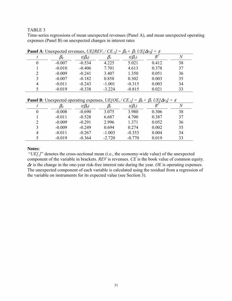
The positive relationship between changes in interest rates and operating income could be

due to a positive effect on revenues or a negative effect on operating expenses. We next rerun the

analysis substituting revenues and operating expenses for operating income. In the first stage

regressions, we use the same instruments as for expected operating income, except that we now

decompose operating income into revenues and operating expenses. The results of the second

stage regressions are presented in Table 3. Similar to the operating-financing decomposition, we

observe positive relations for both revenues and expenses, but the coefficients on revenues are

larger. Thus, unexpected changes in interest rates should revise expectations of current and near

future revenues, expenses and earnings in the direction of the interest rate change.

14

4. Interest rates and equity value

Primary analysis

The results of the previous section suggest that changes in interest rate have a positive effect on

expected payoffs to holding stocks. They do not reveal, however, the extent to which the change

in expected payoffs offsets the negative discount rate effect. We next investigate the net effect of

changes in interest rates on equity value. To this end, we refer to the residual income valuation

model (see Appendix 1) which expresses equity value as the sum of current book value and

discounted expected risk-adjusted residual earnings (that is, earnings in excess of required

earnings on the book value of the investment involved in generating the earnings). Under this

model, changes in interest rates may affect value by changing either expected residual earnings

or the rate at which the residual earnings are discounted.13 Because they have a positive effect on

the discount rate, changes in interest rates may have a non-negative effect on equity value only if

their effect on expected residual earnings is positive and large enough to fully offset the discount

rate effect. Accordingly, we investigate the relationship between changes in interest rates and

subsequent residual earnings.

To preface the analysis, we first replicate the research on stock returns and interest rates

for our sample. Monthly excess returns (over the risk-free interest rate) for a value-weighted

portfolio of all NYSE and AMEX stocks from 1964 to 2001 are regressed on contemporaneous

changes in interest rates. Four measures of interest rates are used: the artificial yields on Treasury

discount bonds with one and five years to maturity, and the yields on constant maturity Treasury

bonds with ten and thirty years to maturity.14 An implicit assumption in these regressions is that

the expected change in interest rates during the month is zero. To examine whether this

assumption is a reasonable approximation, we also regress the excess market return on the

15

unexpected change in the one-year Treasury rate, estimated using the one year rate at the end of

the month and the term structure at the beginning of the month.

The results are reported in Table 4. As the mean values of changes in interest rates are

relatively small, the intercepts approximate the average monthly market risk premium over the

risk-free rate (about 6 percent annually). The results for the total and unexpected change in the

one-year interest rate are similar, indicating that changes in interest rates are largely unexpected.

The slope estimates are negative for all maturities (and significantly so): Stock returns, in the

aggregate, are negatively related to changes in interest rates. Is this relationship consistent with

fundamentals?

[Insert Table 4 here]

To examine the information in interest rate changes about expected residual earnings, we

re-estimate the two-stage model described in Section 3, substituting residual earnings for

earnings. Panel A of Table 5 report the second stage estimation results. The estimated coefficient

on the unexpected change in interest rates (β1) is positive and significant for the current year (t =

0) but negative for all subsequent years (significant for t = 2 and 3).

[Insert Table 5 here]

To assess the overall effect of changes in interest rates on expected residual earnings, we

re-estimate the first and second stage regressions substituting the sum of residual earnings in

years 0 through t for residual earnings in year t. Panel B of Table 5 reports the results of the

second stage regressions. As shown, the slope coefficient in the second stage regressions is

negative from t = 2, and significant from t = 4. These results indicate that the positive current

year effect only partially offsets the negative future years effect, and so the overall effect of

changes in interest rates on subsequent residual earnings is negative.

16

These findings are consistent with the negative association between changes in interest

rates and stock returns. Interest rates are negatively related to stock prices not only because they

have a positive effect on the discount rates used in the (market) capitalization of residual

earnings, but also because they are negatively related to residual earnings.

Residual operating income and residual Interest expense

In the previous section, we have shown that changes in interest rates are negatively related to

subsequent residual earnings, and interpreted this result as indicating that interest rate changes

have a negative effect on equity value. This inference assumes that the riskiness of residual

earnings remains unchanged (see Appendix 1). However, to the extent that changes in interest

rates trigger changes in financial leverage, the riskiness of residual earnings is likely to change.

In particular, if an increase in interest rates leads to a decrease in financial leverage, the riskiness

of residual earnings will decrease. Thus, the negative effect of interest rate changes on residual

earnings documented in the previous section may not imply a negative effect on expected risk-

adjusted residual earnings.

To address this concern, we examine the effect of changes in interest rates on the values

of operations and net financial obligations separately. Specifically, we re-estimate the two-stage

regression model with residual operating income (operating income minus the book value of net

operating assets charged by the risk-free rate) and residual interest expense (net interest expense

minus net financing debt times the risk-free rate).15 In contrast to residual earnings, the riskiness

of residual operating income and residual interest expense is not directly affected by changes in

financial leverage. We focus on the effect on cumulative residual operating income and

cumulative residual interest expense. The results of the second stage regressions are reported in

Table 6.

17

[Insert Table 6 here]

It is evident that unexpected changes in interest rates are negatively related to unexpected

residual operating income over the six years (Panel A, the t = 5 regression). Thus, increases in

interest rates indicate smaller residual operating income and larger discount rates, both implying

a negative effect on the value of operations. In contrast, the overall effect of changes in interest

rates on residual interest expense is insignificant (Panel B, the t = 5 regression). Since the mean

value of residual interest expense is very small (0.2% of the book value of equity), the discount

rate effect on the value of net financing debt is also likely to be small (zero divided by any non-

zero number is zero).16 Therefore, we conclude that the change in the value of debt is

substantially smaller (in magnitude) than the change in the value of operations, consistent with

the results of the residual earnings analysis in Table 5.

Profitability, excess profitability and growth

Residual earnings in year t can be decomposed as follows:

REt ≡ Et – rt-1 × CEt-1

= (ROCEt – rt-1) × CEt-1

= (ROCEt – rt-1) × GROWTH-1,t-1 × CE-1,

where ROCEt ≡ Et / CEt-1 is return on common equity in year t; rt-1 is the risk-free spot rate at the

beginning of year t; ROCEt – rt-1 is excess profitability in year t; and GROWTH-1,t-1 ≡ CEt-1/ CE-1

is one plus the growth rate in the book value of common equity from the beginning of the interest

rate change year (time –1) through the beginning of year t (time t–1). Thus, changes in interest

rates may revise expectations of residual earnings by changing expected excess profitability,

expected growth, or the covariance between them. Changes in excess profitability could be due

18

to changes in profitability or in the expected spot rate. In this section, we examine the

information in interest rate changes about these determinants of residual earnings.

We use the same two-stage approach developed in Section 3. Table 7 presents estimation

results for the second stage. As shown in Panel A, unexpected changes in interest rates in year 0

are positively and significantly related to unexpected ROCE in years 0 and 1 and insignificantly

related to unexpected ROCE in years 3, 4 and 5. Moreover, the coefficient for year 0 is

approximately one, suggesting that changes in the one-year interest rate are fully offset by a

corresponding change in ROCE in the same year. In contrast, excess ROCE in Panel B is

negatively related to changes in interest rates in all future years (significant relations for t = 2, 3

and 4). The regressions in Panel C, which examine the information in changes in the one-year

spot rate for its future levels, help explain these results. Changes in interest rates are on average

more permanent than changes in profitability (compare the β1 coefficients in Panel C with those

in Panel A), and are therefore negatively related to subsequent excess profitability (in Panel B).

[Insert Table 7 here]

In Panel D of Table 7, we report the results for cumulative growth. Unexpected

cumulative growth in book value for t = 1, 2 and 3 is positively and significantly related to

unexpected changes in interest rates in year 0. This is not surprising. Growth in common equity

may be related to ROCE, which is positively related to changes in interest rates. Thus, the

positive relationship between changes in interest rates and unexpected earnings documented in

Table 2 is due to positive effects on both profitability and growth in book value.

Distinguishing effects of real interest rates and expected inflation

According to Fisher (1930), changes in nominal interest rates are due to changes in expected

inflation and/or to changes in the real rate of interest. Section 2 indicates that changes in interest

19

rates due to changes in expected inflation may have different effects on expected current and

future earnings than those due to changes in the real rate of interest. To distinguish the two

effects, therefore, we decompose the unexpected change in nominal rates into expected inflation

and real rate components, and re-run the regressions. We measure expected inflation using the

mean expected growth in the consumer price index over the next 12-months from the Livingston

survey.17 We use this series to estimate the change in the expected inflation and real rate

components of the one-year interest rate. Next, to remove the expected component of these

variables, we orthogonalize them with respect to the first stage instruments.

Table 8 presents the results of estimating the following second-stage equation with the

cross-sectionally averaged variables:

UE[�t

jRE0

/ CE-1] = β0 + β1 UE[∆rr0] + β2 UE[∆E(INF)0] + ε (3)

for t = 0, 1, 2, 3, 4, 5, where UE[∆rr0] (UE[∆E(INF)0]) measures the unexpected change in the

real rate (expected inflation) component of the one-year interest rate during year 0.

[Insert Table 8 here]

The overall effect of changes in expected inflation and real rates on residual earnings is

negative (the t = 5 regression). As the discount rate effect of both changes is also negative, we

conclude that changes in interest rates have a negative effect on equity value independent of

whether they are due to changes in expected inflation or changes in real rates. However,

compared with real rates, changes in expected inflation have a relatively delayed, less negative

and less significant relationship with expected residual earnings.18

20

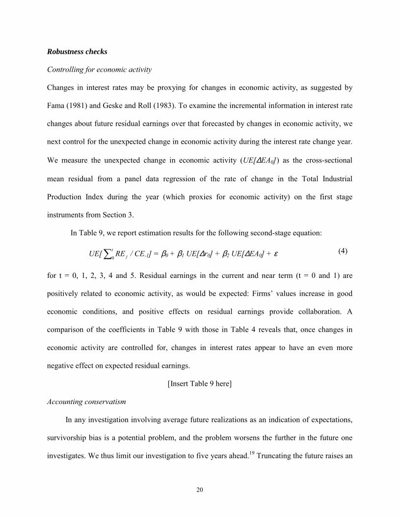
Robustness checks

Controlling for economic activity

Changes in interest rates may be proxying for changes in economic activity, as suggested by

Fama (1981) and Geske and Roll (1983). To examine the incremental information in interest rate

changes about future residual earnings over that forecasted by changes in economic activity, we

next control for the unexpected change in economic activity during the interest rate change year.

We measure the unexpected change in economic activity (UE[∆EA0]) as the cross-sectional

mean residual from a panel data regression of the rate of change in the Total Industrial

Production Index during the year (which proxies for economic activity) on the first stage

instruments from Section 3.

In Table 9, we report estimation results for the following second-stage equation:

UE[�t

jRE0

/ CE-1] = β0 + β1 UE[∆r0] + β2 UE[∆EA0] + ε (4)

for t = 0, 1, 2, 3, 4 and 5. Residual earnings in the current and near term (t = 0 and 1) are

positively related to economic activity, as would be expected: Firms’ values increase in good

economic conditions, and positive effects on residual earnings provide collaboration. A

comparison of the coefficients in Table 9 with those in Table 4 reveals that, once changes in

economic activity are controlled for, changes in interest rates appear to have an even more

negative effect on expected residual earnings.

[Insert Table 9 here]

Accounting conservatism

In any investigation involving average future realizations as an indication of expectations,

survivorship bias is a potential problem, and the problem worsens the further in the future one

investigates. We thus limit our investigation to five years ahead.19 Truncating the future raises an

21

additional issue, however. To the extent that interest rate changes are associated with investment,

the regression estimates may be biased due to conservative accounting, which reduces earnings

during the early years following investments and increases them subsequently.20 We therefore

rerun the analysis excluding firms that typically apply conservative accounting. We use three

variables to identify such firms: (1) the ratio of research and development (R&D) plus

advertising expenses to sales in the year prior to the interest rate change; (2) the price-to-book

ratio at the beginning of the year of the interest rate change; and (3) the rate of growth in book

value in the year prior to the interest rate change. R&D and advertising costs are expensed as

incurred and so firms with high levels of R&D and advertising costs are more strongly affected

by conservative accounting. High price-to-book ratios are indicative of conservative accounting

because assets are excluded from the balance sheet. Growth serves as a filter because

conservative accounting has a greater effect on earnings during growth periods.

Accordingly, we re-estimate the regressions excluding all firm-year observations for

which the R&D and advertising were more than 2% of sales, the price-to-book ratio was above

the 75th percentile in each year, or growth in NOA was greater than 20%. The results were

similar to those obtained with the full sample. We obtained similar results also when excluding

firm-year observations with any R&D or advertising expense, and for all price-to-book quartiles.

Hence we conclude that our inferences are not due to the effects of conservative accounting.

Alternative measurements

In all the analyses thus far, we have focused on the change in the one-year interest rate. This

choice makes it easier to interpret the results because we measure earnings and profitability using

annual data. To check the sensitivity of the results to the use of alternative interest rates, we

rerun the analyses measuring the change in interest rates using each of the following three

22

variables instead of the change in the one year rate: (1) the change in the five year spot rate, (2)

the change in the yield on constant maturity Treasury bonds with ten years to maturity, and (3)

the difference between the one-year Treasury rate at the end of the year and the corresponding

forward rate at the beginning of the year. In all cases, we obtain results similar to those reported.

To construct the second stage variables, we calculated the cross-sectional means of the

residuals from the first stage panel data regressions. This approach assigns the same weight to

each firm. To check the robustness of the results, we rerun all the analyses using cross-sectional

weighted means of the first stage residuals. That is, each residual is given a weight proportional

to the value of a weight variable. We use three alternative weight variables: the market and book

values of equity, and the book value of total assets, measured at the beginning of the interest rate

change year. In all cases, we obtain results similar to those reported above.

5. Conclusion and discussion

This paper has examined the relationship between changes in interest rates, earnings and

equity value. Changes in interest rates are positively related to unexpected earnings, but this

effect only partially offsets the negative value effect of the change in required returns. Hence, the

overall effect of changes in interest rates on equity value is negative, consistent with the negative

correlation between changes in interest rates and stock returns.

The analysis yields further interesting insights. Interest rates are positively related to

revenues, operating expenses and net interest expense, but the effect on revenue is the dominant

one. Also, an increase in the one-year interest rate predicts a similar increase in same year

profitability, but the change in profitability is less persistent than the interest rate change.

Consequently, changes in interest rates are negatively related to subsequent excess profitability

23

and residual earnings. These findings have implications for practitioners and researchers who

forecast or use forecasts of earnings for equity valuation, performance evaluation or other

objectives. Changes in interest rates convey information about subsequent revenues, expenses,

earnings and profitability, and should therefore be incorporated in such analyses.

The negative relationship between changes in interest rates and residual earnings is not

due to interest rates proxying for economic activity; after controlling for changes in economic

activity, the relationship becomes even more negative. In addition, the directional effects are

similar for changes in the expected inflation and real components of nominal interest rates.

Accordingly, our analysis indicates that contrary to the traditional view, equities do not provide a

complete hedge against changes in inflation (nor against changes in real interest rates).

Our tests cover only five years after the interest rate change, so the inference that the

effect on future residual earnings is negative is made with some reservation.21 We expect that, as

firms make new investments, they would do so to cover the hurdle rates demanded by the

changed interest rates. Accordingly one can interpret the negative relationship between changes

in interest rates and residual earnings over the subsequent five years as due to the effect on

investment in place.22 This inference is supported by the pattern of the relationship between

residual earnings and interest rates. Between years 2 and 5 after the interest rate change, the

effect on residual earnings becomes gradually weaker, consistent with the increase in the

proportion of new investments (which do not generate negative residual earnings).

The results are for all firms, on average. In the vein of Bernard (1986), further research

may find varying sensitivities to changes in expected inflation and real interest rates among

firms. For example, the negative effect of changes in expected inflation on subsequent residual

earnings may be delayed for firms with mostly fixed costs, which reflect inflation with a lag. On

24

the other hand, such firms typically have many long-term assets in place, which are costly to

reallocate in response to interest rate shocks. Future research may also decompose earnings to

identify which components are particularly sensitive to interest rate changes (e.g., cost of goods

sold, SG&A or income taxes), and in which circumstances. Such research would broaden our

knowledge of the association between changes in interest rates and value drivers and help in the

application of fundamental valuation techniques to specific firms.

25

Appendix 1: Valuation models and stochastic interest rates

The dividend discount model prices expected dividends at the present date, t, on the basis of information at that date as

�∞

+=

+=1tτ tτ

ττtτtt R

)Q~,d~(Cov)d~(EP ,

where dτ is net dividends (dividends plus share repurchases and minus share issues) paid in period τ; Rtτ is the riskless return on a dollar invested from date t through date τ (one plus the risk free rate of return, rtτ), which captures the time value of money; Et and Covt are expectations and covariances, respectively, from a fixed set of beliefs at date t; and τQ~ is an index that captures the relative desirability of payoffs in the different states of nature.23

Feltham and Ohlson (1999) show that the expression of price in terms of expected dividends can be restated in terms of the current book value of common equity (CEt), and the expected stream of future residual earnings (REτ, τ > t). Residual earnings are earnings (E) charged by the product of the beginning-of-period book value and the (uncertain) risk free spot rate, r (i.e., REτ ≡ Eτ – rτ CEτ-1). Given clean-surplus accounting such that dτ = Eτ – (CEτ – CEτ-1) for every state in which dividends are realized at each future date τ,

�∞

+=

++=1tτ tτ

ττtτttt R

)Q~,(RECov)(REECEP ,

provided ( ) ∞→→ τas 0RCEE tττt .

Both models accommodate stochastic interest rates. The denominator effect of changes in interest rates reduces the present value of expected risk-adjusted dividends or residual earnings. The numerator effect, on which we focus, changes the levels of expected risk-adjusted dividends or residual earnings.24 We focus on expected residual earnings. We assume that the only effect on the covariance term is due to the change in the magnitude of residual earnings.25 Hence, the change in the numerator is proportional to the change in expected residual earnings, and the directional effect on the numerator is the same as that on expected residual earnings. In more standard terminology, we assume that changes in interest rates do not affect the “risk premium” over the risk-free rate (or the discount for risk).26 In Section 4, we address the possibility of a change in the covariance due to a change in leverage by examining effects on operations separately from effects on financial items.

26

Appendix 2: Notation and variables measurement

This appendix describes how the variables are measured.

Financial assets = cash and short-term investments (Compustat #1) plus investments and advances-other (#32).

Financial liabilities = debt in current liabilities (#34) plus long-term debt (#9) plus preferred stock (#130) minus preferred treasury stock (#227) plus preferred dividends in arrears (#242) plus minority interest (#38). (Minority interest is treated as an obligation here; for an alternative minority sharing treatment (that considerably complicates the presentation), see Nissim and Penman (2001). Tests show that the treatment has little effect on the results.)

Net Financing debt = financial liabilities minus financial assets.

Common equity (CE) = common equity (#60) plus preferred treasury stock (#227) minus preferred dividends in arrears (#242).

Net operating assets = net financing debt plus common equity.

Net interest expense (NIE) = after-tax interest expense (#15 × (1 – marginal tax rate)) plus preferred dividends (#19) minus after-tax interest income (#62 × (1 – marginal tax rate)) plus minority interest in income (#49) minus the change in marketable securities adjustment (change in #238). (See comment regarding the treatment of minority interest in the calculation of Financial Obligations above.)

Earnings (E, comprehensive net income) = net income (#172) minus preferred dividends (#19) plus the change in marketable securities adjustment (change in #238) plus the change in cumulative translation adjustment (change in #230).

Operating income (OI) = net interest expense plus earnings.

Marginal tax rate = the top statutory federal tax rate plus 2% average state tax rate. The top federal statutory corporate tax rate was 52% in 1963, 50% in 1964, 48% in 1965-1967, 52.8% in 1968-1969, 49.2% in 1970, 48% in 1971-1978, 46% in 1979-1986, 40% in 1987, 34% in 1988-1992 and 35% in 1993-2001.

27

References

Ang, A., and J. Liu. 2001. A general affine earnings valuation model. Review of Accounting Studies 6 (4): 397-425.

Beaver, W., and S. Ryan. 2000. Biases and lags in book value and their effects on the ability of the book-to-market ratio to predict book return on equity. Journal of Accounting Research 38 (1): 127-148.

Bernard, V. L. 1986. Unanticipated inflation and the value of the firm. Journal of Financial Economics 15 (3): 285-321.

Bodie, Z. 1976. Common stocks as a hedge against inflation. Journal of Finance 31 (2): 459-470.

Campbell, J. Y., and J. Ammer. 1993. What moves the stock and bond markets? A variance decomposition for long-term asset returns. Journal of Finance 48 (1): 3-37.

Domian, D. L., J. E. Gilster, and D. A. Louton. 1996. Expected inflation, interest rates, and stock returns. The Financial Review 31 (4): 809-830.

Ewing, B. T., J. E. Payne, and S. M. Forbes. 1998. Co-movements of the prime rate, CD rate, and the S&P financial stock index. The Journal of Financial Research 21 (4): 469-482.

Fama, E. F. 1981. Stock returns, real activity, inflation, and money, American Economic Review 71 (4): 545-565.

Fama, E. F. 1990. Stock returns, expected returns, and real activity. Journal of Finance 45 (4): 1089-1108.

Fama, E. F., and K. R. French. 1989. Business conditions and expected returns on stock and bonds. Journal of Financial Economics 25 (1): 23-49.

Fama, E. F., and G. W. Schwert. 1977. Asset returns and inflation. Journal of Financial Economics 5 (2): 115-146.

Feldstein, M. 1980. Inflation, tax rules and the stock market. Journal of Monetary Economics 6 (3): 309-331.

Feltham, G. A., and J. A. Ohlson. 1995. Valuation and clean surplus accounting for operating and financial activities. Contemporary Accounting Research 11(2): 689-731.

Feltham, G. A., and J. A. Ohlson. 1999. Residual earnings valuation with risk and stochastic interest rates. The Accounting Review 74 (2): 165-183.

Fisher, I. 1930. The Theory of Interest. New York: McMillan.

Flannery, M. J., and C. M. James. 1984. The effect of interest rate changes on the common stock returns of financial institutions. Journal of Finance 39 (4): 1141-1153.

28

Geske, R., and R. Roll. 1983. The fiscal and monetary linkage between stock returns and inflation. Journal of Finance 38 (1): 1-33.

Gode, D., and J. Ohlson. 2002. Accounting-based valuation with changing interest rates. Working paper, New York University.

Hess P. J., and B. Lee. 1999. Stock returns and inflation with supply and demand disturbances. Review of Financial Studies 12 (5): 1203-1218.

Huang, C., and R. H. Linzenberger. 1988. Foundations for Financial Economics. New York: North-Holland.

Kothari, S. P. 2001. Capital markets research in accounting. Journal of Accounting and Economics 31 (1-3): 105-231.

Lintner, J. 1975. Inflation and security returns. Journal of Finance 30 (2): 259-280.

Lucas Jr., R. E. 1978. Asset prices in an exchange economy. Econometrica 46 (6): 1429-1446.

Miller, M. H., and F. Modigliani. 1961. Dividend Policy, Growth and the Valuation of Shares. Journal of Business 34 (4): 411-433.

Modigliani, F., and R. A. Cohn. 1979. Inflation, rational valuation and the market. Financial Analyst Journal 35 (2): 24-44.

Nissim, D., and S. H. Penman. 2001. Ratio analysis and equity valuation: From research to practice. Review of Accounting Studies 6 (1): 109-154.

Ohlson, J.A. 1999. Conservative accounting and risk. Working paper, New York University.

Penman, S. H., and T. Sougiannis. 1998. A comparison of dividend, cash flow, and earnings approaches to equity valuation. Contemporary Accounting Research 15 (3): 343-383.

Ritter, J. R., and R. S. Warr. 2001. The decline of inflation and the bull market of 1982 to 1999. Journal of Financial and Quantitative Analysis (forthcoming).

Sharpe, S. A. 2001. Reexamining stock valuation and inflation: The implications of analysts’ earnings forecasts. The Review of Economics and Statistics (forthcoming).

Shiller, R. J., and A. E. Beltratti. 1992. Stock prices and bond yields: Can their comovements be explained in terms of present value models? Journal of Monetary Economics 30 (1): 25-46.

Williams, J. 1938. The Theory of Investment Value. Cambridge: Harvard University Press.

Zhang, X-J. 2000. Conservatism, growth, and the analysis of line items in earnings forecasting and valuation. Working paper, University of California, Berkeley.

29

TABLE 1 Panel data regressions of earnings on instruments for expected earnings

εααααααααα +++++++++=−

−−−−−−

−

−

−

− 181716151413

1

12

1

110

1

11051CE

INFEArrrCE

MVCECEE

CEEt

t α0 α1 α2 α3 α4 α5 α6 α7 α8 R2 N 0 -0.005 0.468 0.019 -1.092 1.643 -0.799 0.303 0.851 -0.037 0.262 36,687 -1.421 89.115 40.154 -8.426 4.295 -2.720 15.830 20.450 -2.484 1 0.030 0.364 0.020 -1.816 1.302 -0.088 0.250 1.008 0.074 0.142 34,010 7.101 52.019 34.034 -10.836 2.687 -0.241 10.478 19.187 3.960 2 0.017 0.320 0.024 -3.883 3.352 -0.333 0.376 1.597 0.122 0.110 31,586 3.276 35.906 32.770 -19.395 5.724 -0.750 13.224 25.470 5.405 3 0.022 0.292 0.030 -5.615 7.082 -2.705 0.350 2.180 0.162 0.103 29,298 3.613 26.153 33.334 -24.170 10.554 -5.337 10.659 29.820 6.206 4 0.053 0.283 0.037 -4.917 6.863 -3.333 0.180 2.133 0.265 0.094 27,201 7.341 20.459 33.865 -17.876 8.743 -5.657 4.705 24.678 8.647 5 0.061 0.330 0.042 -5.796 12.375 -7.999 0.178 2.383 0.322 0.095 25,286 7.217 19.657 32.647 -18.132 13.540 -11.660 4.006 23.808 8.951

Notes: t-statistics are reported below the coefficient estimates. E is earnings (comprehensive net income to common equity). CE is the book value of common equity. MVCE is the market value of common equity. r1 and r5 measure the artificial yield on Treasury discount bonds with one and five years to maturity, respectively. r10 measures the yield on constant maturity Treasury bonds with ten years to maturity. EA is the growth rate in the industrial production index during the year. INF is the rate of inflation during the year. N is the number of firm-year observations in the pooled time series and cross-sectional regressions.

30

TABLE 2 Time-series regressions of mean unexpected earnings (Panel A), mean unexpected operating income (Panel B), and mean unexpected net interest expense (Panel C) on unexpected changes in interest rates Panel A: Unexpected earnings, UE[Et / CE-1] = β0 + β1 UE[∆r0] + ε

t β0 t(β0) β1 t(β1) R2 N 0 0.001 0.473 1.015 5.275 0.436 38 1 0.002 0.322 0.835 2.406 0.142 37 2 0.002 0.361 0.154 0.399 0.005 36 3 0.002 0.374 -0.140 -0.388 0.005 35 4 0.000 0.047 -0.466 -1.029 0.032 34 5 -0.001 -0.136 -0.639 -1.449 0.063 33

Panel B: Unexpected operating income, UE[OIt / CE-1] = β0 + β1 UE[∆r0] + ε

t β0 t(β0) β1 t(β1) R2 N 0 0.001 0.206 1.089 6.021 0.502 38 1 0.001 0.107 1.056 2.989 0.203 37 2 0.001 0.166 0.381 0.902 0.023 36 3 0.001 0.208 0.064 0.156 0.001 35 4 0.000 -0.003 -0.241 -0.483 0.007 34 5 -0.001 -0.086 -0.541 -1.115 0.039 33

Panel C: Unexpected net interest expense, UE[NIEt / CE-1] = β0 + β1 UE[∆r0] + ε

t β0 t(β0) β1 t(β1) R2 N 0 -0.001 -0.740 0.083 1.679 0.073 38 1 -0.001 -0.693 0.255 3.564 0.266 37 2 -0.001 -0.457 0.270 2.703 0.177 36 3 0.000 -0.196 0.166 1.379 0.055 35 4 0.000 0.010 0.132 0.958 0.028 34 5 0.000 0.119 0.090 0.597 0.011 33

Notes: “UE[.]” denotes the cross-sectional mean (i.e., the economy-wide value) of the unexpected component of the variable in brackets. E is earnings (comprehensive net income to common equity). CE is the book value of common equity. OI is operating income. ∆r is the change in the one-year risk-free interest rate during the year. NIE is net interest expense. The unexpected component of each variable is calculated using the residual from a regression of the variable on instruments for its expected value (see Section 3).

31

TABLE 3 Time-series regressions of mean unexpected revenues (Panel A), and mean unexpected operating expenses (Panel B) on unexpected changes in interest rates Panel A: Unexpected revenues, UE[REVt / CE-1] = β0 + β1 UE[∆r0] + ε

t β0 t(β0) β1 t(β1) R2 N 0 -0.007 -0.534 4.225 5.021 0.412 38 1 -0.010 -0.406 7.701 4.613 0.378 37 2 -0.009 -0.241 3.407 1.350 0.051 36 3 -0.007 -0.182 0.858 0.302 0.003 35 4 -0.011 -0.243 -1.001 -0.315 0.003 34 5 -0.019 -0.338 -3.224 -0.815 0.021 33

Panel B: Unexpected operating expenses, UE[OEt / CE-1] = β0 + β1 UE[∆r0] + ε

t β0 t(β0) β1 t(β1) R2 N 0 -0.008 -0.690 3.075 3.980 0.306 38 1 -0.011 -0.528 6.687 4.700 0.387 37 2 -0.009 -0.291 2.996 1.371 0.052 36 3 -0.009 -0.249 0.694 0.274 0.002 35 4 -0.011 -0.267 -1.003 -0.353 0.004 34 5 -0.019 -0.364 -2.720 -0.770 0.019 33

Notes: “UE[.]” denotes the cross-sectional mean (i.e., the economy-wide value) of the unexpected component of the variable in brackets. REV is revenues. CE is the book value of common equity. ∆r is the change in the one-year risk-free interest rate during the year. OE is operating expenses. The unexpected component of each variable is calculated using the residual from a regression of the variable on instruments for its expected value (see Section 3).

32

TABLE 4 Regressions of monthly excess market return on changes in interest rates

Intercept ∆r1 UE_∆r1 ∆r5 ∆r10 ∆r30 R2 N

0.005 -1.513 0.035 456 2.320

-4.072

0.005 -1.580 0.038 456 2.193

-4.247

0.005 -2.516 0.050 456 2.378

-4.870

0.005 -3.824 0.072 456 2.434

-5.936

0.006 -3.431 0.057 297 2.510 -4.242

Notes: t-statistics are reported below the coefficient estimates. The dependent variable, excess market return, is the difference between the monthly value-weighted return including all distributions on NYSE and AMEX firms and the yield (bid-ask average) on the one-month Treasury issue at the beginning of the month. ∆r1 and ∆r5 measure the monthly change in the artificial yield on Treasury discount bonds with one and five years to maturity, respectively. UE_∆r1 is the unexpected change during the month in the one-year Treasury rate calculated using the one-year rate at the end of the month and the term structure at the beginning of the month. ∆r10 and ∆r30 measure the monthly change in the yield on constant maturity Treasury bonds with ten and thirty years to maturity, respectively. The period covers January 1964 through December 2001. The thirty years rate is available only since March 1977.

33

TABLE 5 Time-series regressions of economy-wide unexpected residual earnings on unexpected changes in interest rates Panel A: Unexpected residual earnings in year t, UE[REt / CE-1] = β0 + β1 UE[∆r0] + ε

t β0 t(β0) β1 t(β1) R2 N 0 0.001 0.494 1.058 5.300 0.438 38 1 0.002 0.358 -0.304 -0.886 0.022 37 2 0.002 0.451 -0.842 -2.502 0.156 36 3 0.001 0.259 -0.828 -2.326 0.141 35 4 -0.001 -0.198 -0.710 -1.430 0.060 34 5 -0.002 -0.208 -0.538 -1.024 0.033 33

Panel B: Unexpected cumulative residual earnings from year 0 through year t, UE[�

tjRE

0/ CE-1] = β0 + β1 UE[∆r0] + ε

t β0 t(β0) β1 t(β1) R2 N 0 0.001 0.494 1.058 5.300 0.438 38 1 0.003 0.412 0.659 1.235 0.042 37 2 0.005 0.449 -0.287 -0.378 0.004 36 3 0.006 0.423 -0.887 -0.977 0.028 35 4 0.003 0.196 -2.000 -1.847 0.096 34 5 0.002 0.099 -2.838 -2.632 0.183 33

Notes: “UE[.]” denotes the cross-sectional mean (i.e., the economy-wide value) of the unexpected component of the variable in brackets. RE is residual earning, calculated as comprehensive income to common equity minus the one-year risk-free interest rate at the beginning of the year multiplied by the book value of common equity (CE) at the beginning of the year. ∆r is the change in the one-year risk-free interest rate during the year. The unexpected component of each variable is calculated using the residual from a regression of the variable on instruments for its expected value (see Section 3).

34

TABLE 6 Time-series regressions of mean unexpected cumulative residual operating income (Panel A) and unexpected cumulative residual interest expense (Panel B) on unexpected changes in interest rates Panel A: Unexpected cumulative residual operating income from year 0 through year t, UE[�

tjROI

0/ CE-1] = β0 + β1 UE[∆r0] + ε

t β0 t(β0) β1 t(β1) R2 N 0 0.001 0.269 1.160 6.082 0.507 38 1 0.002 0.242 0.302 0.575 0.009 37 2 0.003 0.308 -0.991 -1.373 0.053 36 3 0.003 0.241 -1.963 -2.237 0.132 35 4 0.000 -0.021 -2.787 -2.438 0.157 34 5 -0.002 -0.123 -3.325 -2.737 0.195 33

Panel B: Unexpected cumulative residual interest expense from year 0 through year t, UE[�

tjRNIE

0/ CE-1] = β0 + β1 UE[∆r0] + ε

t β0 t(β0) β1 t(β1) R2 N 0 0.000 -0.691 0.090 1.937 0.094 38 1 -0.001 -0.643 -0.289 -2.616 0.164 37 2 -0.001 -0.520 -0.681 -3.513 0.266 36 3 -0.002 -0.474 -0.933 -2.907 0.204 35 4 -0.003 -0.468 -0.792 -1.696 0.083 34 5 -0.004 -0.464 -0.573 -1.029 0.033 33

Notes: “UE[.]” denotes the cross-sectional mean (i.e., the economy-wide value) of the unexpected component of the variable in brackets. ROI is residual operating income, calculated as operating income minus the one-year risk-free interest rate at the beginning of the year multiplied by the book value of net operating assets at the beginning of the year. CE is the book value of common equity. ∆r is the change in the one-year risk-free interest rate during the year. RNIE is residual interest expense, calculated as net interest expense minus the one-year risk-free interest rate at the beginning of the year multiplied by the book value of net financing debt at the beginning of the year. The unexpected component of each variable is calculated using the residual from a regression of the variable on instruments for its expected value (see Section 3).

35

TABLE 7 Time-series regressions of mean unexpected values of determinants of residual earnings on unexpected changes in interest rates

Panel A: Unexpected profitability in year t, UE[ROCEt] = β0 + β1 UE[∆r0] + ε t β0 t(β0) β1 t(β1) R2 N 0 0.001 0.473 1.015 5.275 0.436 38 1 0.002 0.383 0.631 2.083 0.110 37 2 0.002 0.425 -0.009 -0.030 0.000 36 3 0.001 0.371 -0.286 -1.143 0.038 35 4 0.000 0.004 -0.418 -1.504 0.066 34 5 -0.001 -0.170 -0.359 -1.424 0.061 33

Panel B: Unexpected excess profitability in year t, UE[ROCEt – rt-1] = β0 + β1 UE[∆r0] + ε

t β0 t(β0) β1 t(β1) R2 N 1 0.002 0.389 -0.340 -1.120 0.035 37 2 0.002 0.470 -0.784 -2.914 0.200 36 3 0.001 0.237 -0.713 -2.654 0.176 35 4 -0.001 -0.201 -0.564 -1.720 0.085 34 5 -0.001 -0.221 -0.329 -1.027 0.033 33

Panel C: Unexpected spot rate at t-1, UE[rt-1] = β0 + β1 UE[∆r0] + ε t β0 t(β0) β1 t(β1) R2 N 1 N/A N/A 1.000 N/A N/A N/A 2 0.000 0.008 0.784 4.419 0.365 36 3 0.000 0.157 0.440 2.014 0.109 35 4 0.001 0.332 0.137 0.641 0.013 34 5 0.000 0.148 -0.043 -0.202 0.001 33

Panel D: Unexpected cumulative growth in book value from –1 through t–1, UE[GROWTH-1,t-1] = β0 + β1 UE[∆r0] + ε

t β0 t(β0) β1 t(β1) R2 N 1 -0.001 -0.303 1.061 4.642 0.381 37 2 -0.001 -0.155 1.330 2.287 0.133 36 3 0.000 0.026 1.568 1.804 0.090 35 4 0.003 0.160 1.409 1.277 0.048 34 5 0.004 0.189 0.447 0.316 0.003 33

Notes: “UE[.]” denotes the cross-sectional mean (i.e., the economy-wide value) of the unexpected component of the variable in brackets. ROCE is return on common equity, calculated as earnings divided by the book value of common equity (CE) at the beginning of the year. r is the one-year risk-free interest rate, and ∆r is the change in this rate during the year. GROWTHi,j is one plus the cumulative growth in CE from i to j. The unexpected component of each variable is calculated using the residual from a regression of the variable on instruments for its expected value (see Section 3).

36

TABLE 8 Time-series regressions of mean unexpected cumulative residual earnings on unexpected changes in expected inflation and real interest rates UE[�

tjRE

0/ CE-1] = β0 + β1 UE[∆rr0] + β2 UE[∆E(INF)0] + ε

t β0 t(β0) β1 t(β1) β2 t(β2) R2 N 0 0.002 0.501 0.994 4.163 1.234 3.038 0.442 38 1 0.003 0.437 0.325 0.512 1.483 1.483 0.068 37 2 0.005 0.458 -0.517 -0.566 0.285 0.196 0.011 36 3 0.006 0.423 -0.988 -0.901 -0.642 -0.373 0.029 35 4 0.004 0.240 -2.605 -2.037 -0.463 -0.228 0.119 34 5 0.002 0.115 -3.075 -2.383 -2.216 -1.054 0.186 33

Notes: “UE[.]” denotes the cross-sectional mean (i.e., the economy-wide value) of the unexpected component of the variable in brackets. RE is residual earning, calculated as comprehensive income to common equity minus the one-year risk-free interest rate at the beginning of the year multiplied by the book value of common equity (CE) at the beginning of the year. ∆rr is the change in the one-year risk-free real interest rate during the year. ∆E(INF) is the change in expected inflation during the year. The unexpected component of each variable is calculated using the residual from a regression of the variable on instruments for its expected value (see Section 3).

37

TABLE 9 Time-series regressions of mean unexpected cumulative residual earnings on unexpected changes in interest rates, controlling for unexpected changes in economic activity UE[�

tjRE

0/ CE-1] = β0 + β1 UE[∆r0] + β2 UE[∆EA0] + ε

t β0 t(β0) β1 t(β1) β2 t(β2) R2 N 0 0.001 0.364 0.620 2.843 0.322 3.393 0.577 38 1 0.002 0.301 -0.181 -0.321 0.740 2.910 0.233 37 2 0.004 0.360 -1.216 -1.444 0.822 2.154 0.127 36 3 0.004 0.344 -1.792 -1.734 0.784 1.688 0.108 35 4 0.002 0.148 -2.554 -2.017 0.481 0.854 0.117 34 5 0.000 0.020 -3.773 -3.019 0.798 1.417 0.234 33

Notes: “UE[.]” denotes the cross-sectional mean (i.e., the economy-wide value) of the unexpected component of the variable in brackets. RE is residual earning, calculated as comprehensive income to common equity minus the one-year risk-free interest rate at the beginning of the year multiplied by the book value of common equity (CE) at the beginning of the year. ∆r is the change in the one-year risk-free interest rate during the year. ∆EA is the rate of change in the total industrial production index during the year. The unexpected component of each variable is calculated using the residual from a regression of the variable on instruments for its expected value (see Section 3).

38

Endnotes 1 Appendix 1 presents and discusses the model. This formulation, which applies the risk adjustment to expected payoffs in the numerator, contrasts to traditional textbook formulas where the risk adjustment is to the discount rate in the denominator. Risk-adjusted discount rates lack an interpretation that is consistent with no arbitrage. 2 See, for example, Fama and Schwert (1997), Schiller and Beltratti (1992), Campbell and Ammer (1993), and Domian, Gilster and Louton (1996). 3 Lucas (1978) identifies a third determinant of nominal interest rates: a risk premium for the covariance between inflation and consumption growth. 4 Ritter and Warr (2001) and Sharpe (2001) provide some support for the Modigliani and Cohn conjecture. 5 Note also that cash flow from operations, unlike earnings or free cash flow, does not reflect the cost of investment in fixed assets in any period. 6 Due to the aggregation, our estimated coefficients are not exactly identical to those of the one-step approach, but the differences are very small. 7 The consumer price index (all urban, all items) and the total industrial production index were extracted from Standard & Poor’s DRI. 8 Thus, the coefficient on the book value of equity is no longer identifiable (it becomes part of the intercept). 9 This criterion resulted in a loss of approximately 1.9% of the observations. The percentage is larger for the latter years (0.5% for 1964 through 1982 versus 3.2% for 1983 through 2001). 10 Studies have documented that interest rates play an important role in determining financial sector stock prices (e.g., Flannery and James, 1984; Ewing, Payne and Forbes, 1998). 11 In each of the panel data regressions, we delete observations for which any of the firm-specific variables lies outside the 1% to 99% of the pooled distribution. 12 We note that the t-statistics from these regressions are likely overstated, especially those for the macro variables. 13 Changes in interest rates may also change the risk premium. However, we show below that changes in the risk premium due to changes in leverage are not likely to affect our inference. 14 Artificial yields on Treasury discount bonds with one and five years to maturity are extracted from the Fama and Bliss Bond Yield File in CRSP. Yields on treasury securities at constant maturity of 10 and 30 years are extracted from Standard & Poor’s DRI. 15 As with the operating income model in Section 3, we decompose residual earnings and book value into the related operating and financing components.

39

16 In contrast, the mean value of residual operating income (residual earnings) is 4.7% (4.5%) of the book value of equity. 17 This series is available on the web site of the Federal Reserve Bank of Philadelphia (http://www.phil.frb.org/files/liv/datai.html). 18 The delay in the negative effect is not surprising. In periods of inflation, revenues increase contemporaneously with inflation while expenses increase with a lag (e.g., depreciation and amortization, cost of goods sold due to existing inventory, prepaid expenses). 19 Note also that the length of the time-series and hence the efficiency of estimation decrease in the number of future years. 20 See Feltham and Ohlson (1995), Beaver and Ryan (2000), and Zhang (2000) for explanations of how conservative accounting affects accounting profitability. Note that accrual-accounting residual-income valuation (that books investment to the balance sheet) typically mitigates these problems that are extreme with discounted cash flow analysis (that “expenses” all investments). See Penman and Sougiannis (1998). However, GAAP accounting applies cash accounting to expenditures on many “intangible” assets. 21 Extending the analyses to more subsequent years would introduce unacceptable survivorship bias. 22 This argument is perhaps more easily illustrated with bonds. An increase in interest rates lowers the value of a bond held today but does not affect the expected (zero) excess return on a bond to be acquired at the changed interest rate in the future. Similarly, an increase in interest rates results in a capital loss on investments now in place, but is not expected to cause firms to depart from the rule of choosing only those future investments that are expected to cover their required return. In other words, the effect of interest rates changes on excess rates of return from the marginal investment is different from that on the average investments that we document. 23 See Huang and Litzenberger (1988, chapter 7) for a derivation and discussion of the model. 24 Gode and Ohlson (2002) further model the incorporation of stochastic discount rates in accounting-based valuation models. But they model the discount rate, not the numerator effect. Ang and Liu (2001) provide an earnings valuation model with stochastic interest rates that have both numerator and denominator effects. 25 That is, we allow for a scale effect on the covariance, but not for other changes in the distribution of RE. The scale effect is proportional to the change in expected RE because Cov(a×REτ, τQ~ ) = a×Cov(REτ, τQ~ ).

26 One could envision accounting measurements such that “conservative” earnings measurement discounts for risk, and value is given by discounting certainty-equivalent earnings, so measured, without a risk adjustment. See Ohlson (1999).