The Amazon business model, the ... - bohuecon.github.io
188
The Amazon business model, the platform economy and executive compensation: Three essays in search theory
Transcript of The Amazon business model, the ... - bohuecon.github.io

The Amazon business model, the platformeconomy and executive compensation:Three essays in search theory

ISBN: 978 90 361 0563 7
Cover design: Crasborn Graphic Designers bno, Valkenburg a.d. Geul
This book is no. 743 of the Tinbergen Institute Research Series, established through cooperationbetween Rozenberg Publishers and the Tinbergen Institute. A list of books which already ap-peared in the series can be found in the back.

VRIJE UNIVERSITEIT
THE AMAZON BUSINESS MODEL, THE PLATFORM ECONOMY AND EXECUTIVE
COMPENSATION: THREE ESSAYS IN SEARCH THEORY
ACADEMISCH PROEFSCHRIFT
ter verkrijging van de graad Doctor of Philosophy aande Vrije Universiteit Amsterdam,op gezag van de rector magnificus
prof.dr. V. Subramaniam,in het openbaar te verdedigen
ten overstaan van de promotiecommissievan de School of Business and Economicsop donderdag 27 juni 2019 om 11.45 uur
in de aula van de universiteit,De Boelelaan 1105
door
Bo Hu
geboren te Yanzhou, China

promotor: prof.dr. P.A. Gautier
copromotor: dr. M. Watanabe

Acknowledgements
Whenever I think back, I marvel at how right the decision of studying in the Nether-
lands was. It became an unforgettable and enjoyable experience in my life. It is a seven-
year-long journey, but soon I will (and hope to) have my first time of being called Dr.
Hu. Let me take this opportunity to express my gratitude towards the very people who
made it so.
First and foremost, I would like to express my deepest gratitude to my supervisors
Makoto Watanabe and Pieter Gautier. I cannot thank Makoto enough for the supervis-
ing and the coauthoring. I greatly appreciate the time and the energy he invested in
guiding me through my Ph.D. and my job market. I have learned so much from those
hour-long discussions, from he revising my draft, correcting my proofs, etc. He is al-
ways considerate and patient, which makes the Ph.D. life a great memory. I want to
thank Pieter for providing me an inspiring and encouraging environment, and sharing
with me his research networks. With his help, I got the chance to visit the University of
Bristol. His door is always open to whatever questions. His comments and guidance
are reflected everywhere in the chapters. I have learned a lot from him, not only his
infinite knowledge in this field but also his efficiency and concentration.
I would like to express my sincere gratitude to Jose Luis Moraga for his support
from the very beginning to the job market. At a certain point, he acted as a supervisor,
nudging me to participate in seminars, to talk to speakers, telling me the way a good
researcher should follow. He introduced me to the consumer search and switching
workshop in Groningen which opened a new world for me.
Further, I would like to thank Sebastian Gryglewicz, Albert Menkveld, Florian Pe-
ters, Randolph Sloof and Tanja Artiga-Gonzalez for reading and commenting papers
v

vi
that form chapters of this thesis and for their support in my process of searching for
jobs. Randolph was in my Master’s thesis committee. His comments back then in-
spired Chapter 2 of this thesis. Sebastian guided me several times. Albert led me to the
world of market microstructure which is closely related to the topic of the thesis. He
also recommended me in the job market. Tanja suggested that in Chapter 4, I should
use “labor market incentives” rather than “market-based incentives” to refer to the in-
centives of better offers in the managerial labor market. All of the committee members
shared valuable thoughts and comments that significantly improved the thesis.
During my Ph.D. study, I have greatly benefited from my peers, Shuo Xia, Zichen
Deng and Pascal Golec in particular. Special thanks go to Shuo for brainstorming any
time and for sharing his knowledge in Corporate Finance and CEO compensation; to
Zichen for the “two-person reading group” on structure estimation, and for dozens of
research proposals we tried; to Pascal for sharing his thoughts on structure estimation
and his Julia code.
I also benefited a lot from interactions with the economics faculty at the Vrije Uni-
versiteit Amsterdam: Sabien Dobbelaere, Evgenia Motchenkova, Stefan Hochguertel,
Roland Iwan Luttens and Wouter Zant helped me improve my teaching skills; Eric Bar-
telsman and Aico van Vuuren recommended me in the job market; Bas van der Klaauw
and Bjorn Brugemann guided me with their expertise; Maarten Lindeboom gave me
the refereeing opportunity; Chris Elbers offered me a chance to work in field experi-
ments; and Mauro Mastrogiacomo, Xiaoming Cai, Cindy Chen, Iulian Ciobica, Piotr
Denderski, Xinying Fu, Nynke de Groot, Patrick Hullegie, Nadine Ketel, Philipp Kol-
lenda, Simas Kucinskas, Yue Li, Emil Mihaylov, Paul Muller, Florian Sniekers, Sandor
Sovago, Yajie Sun, Jurre Thiel, Coen van de Kraats, Martin Wiegand, Jochem Zweerink
and others for fun chats. I would like to thank Jochem in particular for translating the
summary of the thesis into Dutch.
I would also like to thank Gregory Jolivet, Helene Turon and Gerard van den Berg
for hosting my visit to the University of Bristol where I started my job market paper
(Chapter 4). Ingolf Dittmann from Erasmus University helped me to improve my job
market paper. All staff members of the Tinbergen Institute (TI) and the Economics de-
partment of Vrije Universiteit provided friendly supports which make it an enjoyable

vii
environment to study, research and grow. In particular, I would like to thank Christina
Mansson and Arrianne de Jong for their assistance in my job market; Judith van Kro-
nenburg, Ester van de Bragt, Carolien Stolting, Pienke Dekkers and Trudi Heemskerk
helped me a lot since the very beginning.
I cherish the great memories with all my friends that have not been mentioned
above. Thank you — Hao Fang for all the healing with food and hiking, and for bring-
ing my daughter a gift every time you and Yajing visited us; Albert Jan Hummel, Junze
Sun, Rex Wang, Annti Yang for fighting side by side with me on the job market in
Naples and Atlanta; Wei Li and Heng Ma for so many meals; Wenqian Huang and
Yuan Gu for working through the first year TI homework; Xiao Yu for being my driving
coach; Zhenxing Huang for the guidance on job market; Yuyu Zeng, Yu Gao, Ning Liu,
Simin He, Shihao Yu, Xiao Xiao, Yang Liu, Chen Li, Vitalie Spinu, Jiangyu Ji, Zhiling
Wang, Tong Wang, Yuhao Zhu, Chen Wang, Rui Cai, Tianshi Wang, Junwen Yang,
Yunyu Huang, Xiaona Liu, Qing Wu and Minghui Li for the help and funs throughout
the years. Thanks all for making me feel home here.
My parents, many thanks for the support over the years. You are not only my
parents but also my best friends. You gave me the chance to fly as I wish. I love you.
Yannan, a special big thank you goes to you. Thank you for always being there, which
is so important to me. For so many days and nights that you took care of our daughter
while I was away for conferences or visiting. You supported me firmly in my last two
years while I had no income. You know my ups and downs the best, and you always
support me no matter what decision I make. Muke, each of your smiles is a wonderful
gift for me. Your growth makes me realize how time flies and how slow my research
moves forward. However, since you are growing up so fast, I won’t be too slow.
Sincerely, Bo, in Rotterdam, April 2019

Contents
1 Introduction 1
2 Marketmaking Middlemen 9
2.1 Introduction . . . . . . . . . . . . . . . . . . . . . . . . . . . . . . . . . . . 9
2.2 A basic model with single-market search . . . . . . . . . . . . . . . . . . 15
2.2.1 The framework . . . . . . . . . . . . . . . . . . . . . . . . . . . . . 16
2.2.2 Directed search equilibrium . . . . . . . . . . . . . . . . . . . . . . 20
2.2.3 Participation equilibrium . . . . . . . . . . . . . . . . . . . . . . . 23
2.2.4 Optimal intermediation mode . . . . . . . . . . . . . . . . . . . . 24
2.3 Multi-market search . . . . . . . . . . . . . . . . . . . . . . . . . . . . . . 26
2.3.1 Equilibrium values in the D market . . . . . . . . . . . . . . . . . 27
2.3.2 Directed search equilibrium under multi-market search . . . . . . 28
2.3.3 Intermediation mode . . . . . . . . . . . . . . . . . . . . . . . . . . 31
2.4 Extensions . . . . . . . . . . . . . . . . . . . . . . . . . . . . . . . . . . . . 33
2.4.1 Matching functions . . . . . . . . . . . . . . . . . . . . . . . . . . . 34
2.4.2 Endowment economy . . . . . . . . . . . . . . . . . . . . . . . . . 36
2.4.3 Cost functions . . . . . . . . . . . . . . . . . . . . . . . . . . . . . . 41
2.5 Examples . . . . . . . . . . . . . . . . . . . . . . . . . . . . . . . . . . . . . 43
2.6 Empirical evidence . . . . . . . . . . . . . . . . . . . . . . . . . . . . . . . 47
2.7 Conclusion . . . . . . . . . . . . . . . . . . . . . . . . . . . . . . . . . . . . 49
2.A Omitted proofs . . . . . . . . . . . . . . . . . . . . . . . . . . . . . . . . . 51
2.B Participation fees . . . . . . . . . . . . . . . . . . . . . . . . . . . . . . . . 60
2.C Empirical examination . . . . . . . . . . . . . . . . . . . . . . . . . . . . . 65
3 Competing Intermediaries 71
3.1 Introduction . . . . . . . . . . . . . . . . . . . . . . . . . . . . . . . . . . . 71
viii

CONTENTS
ix
3.2 Setup . . . . . . . . . . . . . . . . . . . . . . . . . . . . . . . . . . . . . . . 75
3.3 Single-market Search . . . . . . . . . . . . . . . . . . . . . . . . . . . . . . 79
3.4 Multi-market Search . . . . . . . . . . . . . . . . . . . . . . . . . . . . . . 80
3.4.1 Directed search equilibrium at incumbent intermediary . . . . . . 81
3.4.2 The best response of the incumbent . . . . . . . . . . . . . . . . . 83
3.4.3 Equilibrium candidate with a pure mode incumbent . . . . . . . 86
3.4.4 The best response of the entrant . . . . . . . . . . . . . . . . . . . 87
3.4.5 Equilibrium analysis . . . . . . . . . . . . . . . . . . . . . . . . . . 90
3.5 Conclusion . . . . . . . . . . . . . . . . . . . . . . . . . . . . . . . . . . . . 94
3.A Omitted proofs . . . . . . . . . . . . . . . . . . . . . . . . . . . . . . . . . 95
3.B The game with a pure middleman entrant . . . . . . . . . . . . . . . . . . 101
4 Managerial Labor Market Competition and Incentive Contracts 103
4.1 Introduction . . . . . . . . . . . . . . . . . . . . . . . . . . . . . . . . . . . 103
4.2 Literature review . . . . . . . . . . . . . . . . . . . . . . . . . . . . . . . . 108
4.3 Motivating facts . . . . . . . . . . . . . . . . . . . . . . . . . . . . . . . . . 111
4.3.1 Size pay-growth premium . . . . . . . . . . . . . . . . . . . . . . . 112
4.3.2 Size incentive premium . . . . . . . . . . . . . . . . . . . . . . . . 114
4.4 The model . . . . . . . . . . . . . . . . . . . . . . . . . . . . . . . . . . . . 116
4.4.1 Ingredients . . . . . . . . . . . . . . . . . . . . . . . . . . . . . . . 117
4.4.2 Optimal contracting problem . . . . . . . . . . . . . . . . . . . . . 122
4.4.3 Equilibrium definition . . . . . . . . . . . . . . . . . . . . . . . . . 124
4.4.4 Contract characterization . . . . . . . . . . . . . . . . . . . . . . . 124
4.4.5 Explaining the size pay-growth premium . . . . . . . . . . . . . . 126
4.4.6 Explaining the size incentive premium . . . . . . . . . . . . . . . 128
4.5 Empirical evidence . . . . . . . . . . . . . . . . . . . . . . . . . . . . . . . 133
4.5.1 Data . . . . . . . . . . . . . . . . . . . . . . . . . . . . . . . . . . . 133
4.5.2 Job-to-job transitions . . . . . . . . . . . . . . . . . . . . . . . . . . 136
4.6 Estimation . . . . . . . . . . . . . . . . . . . . . . . . . . . . . . . . . . . . 141
4.6.1 Numerical method . . . . . . . . . . . . . . . . . . . . . . . . . . . 141
4.6.2 Model specification and parameters . . . . . . . . . . . . . . . . . 141
4.6.3 Moments and identifications . . . . . . . . . . . . . . . . . . . . . 142

xCONTENTS
4.6.4 Estimates . . . . . . . . . . . . . . . . . . . . . . . . . . . . . . . . 144
4.6.5 Predicting firm-size premiums . . . . . . . . . . . . . . . . . . . . 145
4.6.6 Decomposition . . . . . . . . . . . . . . . . . . . . . . . . . . . . . 147
4.7 The long-run trend in executive compensation . . . . . . . . . . . . . . . 147
4.8 The spillover effect and policy implications . . . . . . . . . . . . . . . . . 150
4.9 Conclusions . . . . . . . . . . . . . . . . . . . . . . . . . . . . . . . . . . . 152
4.A Model appendices . . . . . . . . . . . . . . . . . . . . . . . . . . . . . . . . 154
4.B Empirical appendices . . . . . . . . . . . . . . . . . . . . . . . . . . . . . . 157
4.C Estimation . . . . . . . . . . . . . . . . . . . . . . . . . . . . . . . . . . . . 161
Summary 163
Samenvatting (Summary in Dutch) 165
Bibliography 166

List of Figures
2.1 Timing and decisions in single-market search environment . . . . . . . . 19
2.2 Size of middleman sector xm
B (Left) and Price elasticity z(B) (Right) with
Non-linear matching function . . . . . . . . . . . . . . . . . . . . . . . . . 36
2.3 Values of xm − K with single-market search in endowment economy . . 39
2.4 Values of xm − K with multi-market search in endowment economy . . . 40
3.1 Equilibrium under multi-market search . . . . . . . . . . . . . . . . . . . 92
3.2 Comparative Statics w.r.t. λb . . . . . . . . . . . . . . . . . . . . . . . . . . 93
3.3 Comparative Statics w.r.t. B . . . . . . . . . . . . . . . . . . . . . . . . . . 93
4.1 Size premium in performance-based incentives decreases with age . . . 117
4.2 Timing . . . . . . . . . . . . . . . . . . . . . . . . . . . . . . . . . . . . . . 120
4.3 Compare labor market incentives . . . . . . . . . . . . . . . . . . . . . . . 130
4.4 Job-to-job transition rate over age . . . . . . . . . . . . . . . . . . . . . . . 136
4.5 Exit rate over age . . . . . . . . . . . . . . . . . . . . . . . . . . . . . . . . 137
4.6 Distribution of the change of firm size upon job-to-job transitions . . . . 137
4.7 Job-to-job transition rates across firm size . . . . . . . . . . . . . . . . . . 138
4.8 Fraction of market incentives is higher in smaller firms . . . . . . . . . . 148
4.9 Compare higher bids from small/medium firms and from large firms . . 151
4.10 log(delta) over firm size and total compensation . . . . . . . . . . . . . . 157
xi

List of Tables
2.1 Regressions for Amazon’s intermediation mode . . . . . . . . . . . . . . 48
2.2 Summary Statistics . . . . . . . . . . . . . . . . . . . . . . . . . . . . . . . 66
2.3 Correlations among proxy variables . . . . . . . . . . . . . . . . . . . . . 67
2.4 Regressions for Amazon’s intermediation mode using the raw eBay search
results . . . . . . . . . . . . . . . . . . . . . . . . . . . . . . . . . . . . . . . 68
2.5 Regressions for Amazon’s intermediation mode using first 60 characters
to search eBay offers . . . . . . . . . . . . . . . . . . . . . . . . . . . . . . 69
4.1 Pay-growth increases with firm size . . . . . . . . . . . . . . . . . . . . . 113
4.2 Performance-based incentives increase with firm size . . . . . . . . . . . 115
4.3 Summary statistics . . . . . . . . . . . . . . . . . . . . . . . . . . . . . . . 134
4.4 Change of firm size upon job-to-job transitions . . . . . . . . . . . . . . . 139
4.5 Job-to-job transitions and firm size . . . . . . . . . . . . . . . . . . . . . . 140
4.6 Parameters . . . . . . . . . . . . . . . . . . . . . . . . . . . . . . . . . . . . 142
4.7 Moments and estimates . . . . . . . . . . . . . . . . . . . . . . . . . . . . 144
4.8 Predictions on size premiums . . . . . . . . . . . . . . . . . . . . . . . . . 146
4.9 Long-run trend in executive compensation . . . . . . . . . . . . . . . . . 149
4.10 Size incentive premium decreases with executive age . . . . . . . . . . . 158
xii

1Introduction
Why search frictions?
Economics is all about gains from trade. But before gains from trade can be real-
ized, people must meet first. Search frictions characterize the barriers to meet. The
existence of buyers and sellers, who can in principle agree on a price, is not sufficient
for immediate transactions. Agents need to get involved in a costly search process to
find matching partners, and ultimately must decide whether or not to trade now rather
than betting for better trading opportunities in the future.
Most real-world transactions are characterized by these forms of imperfections,
referred as search frictions — consumers search for goods online and offline, workers
search for vacancies, investors search for financial products in an exchange or over the
counter, etc. Search frictions are derived from various sources, including imperfect
information about trading partners, heterogeneous demand and supply, coordination
failures, etc.
1

2
This thesis is among the intellectual efforts to explain the real-world phenomena
through the lens of search theory. However, I leave the comfort zone of search theorists
somewhat and explain issues that are rarely touched. In three chapters, I explore top-
ics ranging from the Amazon business mode (Chapter 2 and Chapter 3) to executive
compensation (Chapter 4).
Why does Amazon combine a middleman and a marketmaker?
Among millions of products available on Amazon, some are sold by Amazon itself,
some are sold by so-called third-party sellers, and the majority are sold by both. This
means, Amazon is a middleman, who specializes in buying and reselling products in its
name, as well as a market-maker, who offers a marketplace (platform) for fees, where
the participating buyers and sellers can search and trade with each other. We thus
call Amazon a Marketmaking Middleman. It is not just Amazon that adopts this hybrid
model. A similar business model has been observed in financial markets. For example,
the New York Stock Exchange (NYSE) took an expanded platform “NYSE Arca” after a
severe market share drop around the year of 2008. In housing markets, the Trump Or-
ganization established a luxury residential real estate brokerage firm, competing with
thousands of housing brokers in New York City.
Why do intermediaries use a hybrid mode? Why has the middleman sector or the
platform not become the exclusive avenue of trade, despite the recent technological
advancements? What determines the position of an intermediary’s optimal mode in
the spectrum spanning from a pure marketmaker mode to a pure middleman mode?
These are the questions answered in Chapter 2 and Chapter 3.
Chapter 2 develops a directed search framework to explain these puzzles. In the
framework, buyers and sellers can search for counter-parties either through an interme-
diated market which is operated by a monopolistic intermediary or via a decentralized
market. The intermediary, who corresponds to a real-world hybrid-mode intermedi-
ary, e.g., Amazon, can make use of both a middleman and a marketmaker sector. The
decentralized market represents an individual’s outside option that creates competitive
pressure on the overall intermediated market.
There exist search frictions in both the intermediated market and the decentral-

CHAPTER 1. INTRODUCTION
3
ized market. While it is not surprising to see a search-frictional decentralized market,
for the intermediated market, one might argue that search frictions should vanish in
a platform-type intermediary like Amazon who provides all sorts of search tools and
price/capacity/review information. Indeed, search frictions in the traditional sense
may fade, but coordination frictions always exist. Burdett et al. (2001) described such
coordination frictions precisely: “(Consider a market where) first sellers set prices, and then
each buyer chooses which seller to visit. There is no search problem in the traditional sense be-
cause buyers know the price and the capacity of each seller with certainty. Still, in equilibrium,
there is a chance that more buyers will show up at a given location than the seller can accommo-
date, in which case some customers get rationed; simultaneously, fewer buyers may show up at
another location than the seller there can accommodate, in which case the seller gets rationed.”
This is the way we model frictions in the intermediated market.
With this framework, the intermediary faces the following trade-off between the
middleman mode and market-maker mode. Compared to an individual seller, a mid-
dleman can hold a larger amount of inventory on the one hand, which reduces out-
of-stock risk and delivers more transactions. On the other hand, activating a platform
attracts sellers to trade in the intermediated market, and ultimately leads to fewer sell-
ers available in the decentralized market. Buyers thus expect a lower outside value
and they are willing to accept less favorable trading terms at the intermediated market.
Accordingly, the intermediary can charge higher price/fees. In a nutshell, the interme-
diary has a trade-off between a larger transaction volume by operating as a middleman
and a higher price/fee by acting as market-maker. This trade-off determines the opti-
mal intermediation mode, and eventually a marketmaking middleman such as Amazon,
who adopts a mixture of these two intermediation modes, can be profit-maximizing.
There are two roles that search frictions play in this trade-off. First, search fric-
tions in the intermediated market highlight the advantage of middleman mode. A
middleman with a much larger inventory can significantly decrease the coordination
frictions — it can simply accommodate the uncertain demands from uncoordinated
buyers. This is perhaps why Amazon invested heavily in building warehouses and
expanding its network of delivery in the passing decades. Second, search frictions in
the decentralized market highlight the advantage of the market-maker mode. Suppose
we assume away search frictions in the decentralized market where there are abundant

4
sellers. Then whatever the intermediated market structure is, with or without an ac-
tive market-maker sector, buyers’ outside value does not change. Hence, the trade-off
between middleman and market-maker modes would not exist.
Our theory is not merely a thought experiment, it has strong real-world support.
We examine the implications of our theory empirically. We take Amazon as the in-
termediated market and eBay as the decentralized market and collect data from both
markets. For our chosen product category, Amazon acts as a marketmaking middle-
man: for 32% of the sample, Amazon acts as a middleman; for the other 68%, Amazon
acts as a platform. Our empirical evidence strongly supports the model’s prediction
that Amazon is more likely to sell the product as a middleman when the chance that a
buyer to meet a seller in eBay is low, the buyers’ bargaining power is low, or the total
demand is high.
Chapter 3 provides an important extension to the baseline model of Chapter 2 on
competing intermediaries. We consider a Bertrand competition game between an in-
cumbent intermediary who can mix a middleman mode and a marketmaker mode,
and an entrant intermediary who is restricted to be a marketmaker. We find that the
entrant faces the choice of being a second-source of intermediation service with high
prices/fees versus being a sole active source with low prices/fees. However, either op-
tion would indicate a positive outside value for buyers, which determines the terms of
trade a buyer is willing to accept at the incumbent. Therefore, the trade-off about inter-
mediation modes in Chapter 2 continues to hold for an intermediary (the incumbent)
in a duopoly. We show that for a reasonable set of parameters, there exists a pure strat-
egy equilibrium where a hybrid incumbent emerges. In this equilibrium, the optimal
(incumbent) intermediation mode features a larger middleman sector when the chance
of a buyer to meet a seller at the entrant intermediary is low, or the total demand is
high. We also show there exists a mixed strategy equilibrium where the incumbent in-
termediary activates its market-maker mode with positive probability. These analyses
serve as theoretical robustness checks for Chapter 2.
Furthermore, the duopoly framework gives a number of new insights. First, we
show that the intermediation structure of the incumbent is an equilibrium result, where
the strategy of the entrant (or outside) intermediary also plays a role. In other words,

CHAPTER 1. INTRODUCTION
5
what shapes the Amazon structure is not only Amazon itself but also other fee-setting
intermediaries such as eBay. Second, the first-mover advantage of the incumbent does
not necessarily lead to a higher market share. In the mixed strategy equilibrium, the
entrant intermediary might be able to undercut and become the sole source for some
category of goods. As a real-world example, the new clothing and fashion online plat-
form Zalando can defeat incumbents like Amazon and eBay and becomes the leading
online shop.
Why do larger firms pay executives more for performance?
Chapter 4 turns to another highly debated issue, the incentive compensation of top
executives. Executives are highly paid, with the majority of their wealth coming from
performance-related rewards, including options and stocks. In this chapter, I aim to
explain a newly documented empirical fact: The firm-size incentive premium. I show
that the executive job ladder which stems from the search frictions in the managerial la-
bor market has a point in explaining the firm-size incentive premium both qualitatively
and quantitatively.
The firm-size incentive premium refers to the fact that the fraction of incentives in
the executive compensation contract increases with firm size. This fact is based on the
executive compensation data in S&P 1500 firms. The contract incentives are measured
by pay-for-performance sensitivity, i.e., for one percent increase in firm value, how
much wealth the executive receives from the compensation package (mainly through
options and stocks). These incentives are believed to be necessary to motivate the ex-
ecutive’s effort and align the interests with that of shareholders.
The chapter starts with a theoretical explanation. In a framework of on-the-job
search, an executive is poached by outside firms. A dynamic incentive contract is de-
signed to deal with both the moral hazard problem inside the firm and the competition
from the external executive labor market. The competition for executives increases total
compensation, and more importantly, it generates a new source of incentives for exec-
utives to exert effort, called labor market incentives, which substitutes for performance-
based incentives embedded in bonus, stocks, options, etc. In the extreme case that
labor market incentives are so large, executives would have the aligned interest with

6
shareholders and take the effort without any incentive pay in the contract. I show that
labor market incentives decrease with firm size. As a result, more performance-based
incentives are required in larger firms.
Why do labor market incentives decrease with firm size? There are two channels in
the model. Here I would like to emphasize the job ladder channel. There is a job ladder
where executives climb from small towards larger firms through job-to-job transitions.
This is so in the data that job-hopping is prevalent and most job-hopping is towards
larger firms. In the model, this happens as the executive auctions his/her labor to
competing firms and the larger firm can bid higher (Postel-Vinay and Robin, 2002).
Now think of an executive in Amazon, who is probably at the top of the job ladder,
and hence he/she receives very little incentives from the labor market. In contrast, an
executive of Netflix should be lower on the job ladder, because he/she can be poached
by larger firms including Amazon, so he/she has larger labor market incentives. Briefly
speaking, the position on the job ladder determines how much labor market incentive
one can get. Executives of larger firms are higher on the job ladder; hence they receive
less from the labor market by climbing the job ladder. If so, then larger firms need to
provide more incentives via the contract to assure the skin in the game. Therefore, the
job ladder effect explains the firm-size incentive premium.
If search frictions are assumed away, this chapter would be a classical career con-
cern story where the executives are motivated to take the effort by his/her labor market
perspective, and this motivation is identical for everyone of the same age (Gibbons and
Murphy, 1992). Indeed, every executive (and every one of us) has a career concern. But
the effect of search frictions clarifies that career concerns are heterogeneous, and are de-
creasing along the job ladder. Through the lens of search frictions, we see that even the
corporate multi-millionaire class is layered, and this structure speaks to the firm-size
incentive premium.
At the end of this chapter, I structurally estimate the theoretical model by the sim-
ulated method of moments. Then I simulate data based on the estimated model and
predict the firm-size incentive premium using the simulated data. I find the prediction
of the model is very close to the incentive premium in the real data. Since there is noth-
ing mechanically to force them to be the same, this shows the model captures some

CHAPTER 1. INTRODUCTION
7
essential feature in the real world.

8

If you can’t beat them, join them.
proverb
2Marketmaking Middlemen
2.1 Introduction
This chapter is based on the working paper co-authored by Pieter Gautier and
Makoto Watanabe.1 It develops a framework in which market structure is determined
by the intermediation service offered to customers. There are two representative modes
of intermediation that are widely used in real-life markets. In one mode, an interme-
diary acts as a middleman (or a merchant), who is specialized in buying and selling for
his own account and typically operates with inventory holdings (e.g. supermarkets,
traditional brick and mortar retailers, and dealers in financial and steel markets). In
the other mode, an intermediary acts as a marketmaker, who offers a marketplace for
fees, where the participating buyers and sellers can search and trade with each other
1We thank seminar and conference participants at U Essex, U Bern, U Zurich, Goergetown U, Albany,the Symposium on Jean Tirole 2014, the Search and Matching workshop in Bristol, SaM network annualconference 2015/2016 in Aix-en-Provence/Amsterdam, Toulouse School of Economics, Tokyo, Rome, the2015 IIOC meeting in Boston, the EARIE 2015 in Munich, the 16th CEPR/JIE conference on Applied Indus-trial Organization, Workshop of the Economics of Platform in Tinbergen Institute, and the 2016 SummerWorkshop on Money, Banking, Payments and Finance in Chicago FED for useful comments.
9

102.1. INTRODUCTION
and at least one side of the market pays a fee for using the platform (e.g. auction sites,
brokers in goods or financial markets, and many real estate agencies).
The market-making mode became more appropriate since new advanced Internet
technology facilitated the use of online platforms in the late 1990s and early 2000s. In fi-
nancial markets, an expanded platform sector is adopted in a specialist market, i.e., the
New York Stock Exchange (NYSE),2 and even in a typical dealers’ (i.e., middlemen’s)
market, i.e the NASDAQ. In goods and service markets, the electronic retailer Ama-
zon.com and the online hotel/travel reservation agency Expedia.com, who have been
a pure middleman, also act as a marketmaker, by allowing other suppliers to partici-
pate in their platform as independent sellers. In housing markets, some entrepreneurs
run a dealer company (developing and owning luxury apartments and residential tow-
ers) and a brokerage company simultaneously in the same market.
Common to all the above examples is that intermediaries operate both as a mid-
dleman and a marketmaker at the same time. This is what we call a marketmaking
middleman. Hence, the first puzzle is to explain the emergence of marketmaking mid-
dlemen, i.e., why the middleman or the platform sector has not become the exclusive
avenue of trade, despite the recent technological advancements.
We also observe considerable differences in the microstructure of trade in these
markets. The NASDAQ is still a more “middlemen-based” market relative to the
NYSE. While some intermediaries in housing markets are marketmaking middlemen,
many intermediaries are brokers. Other online intermediaries, such as eBay and Book-
ing.com, are pure marketmakers, who do not buy and sell on their own accounts, like
Amazon.com and Expedia.com do. They solely concentrate on their platform business.
So the second puzzle is to explain what determines the position of an intermediary’s
optimal mode in the spectrum spanning from a pure marketmaker mode to a pure
middleman mode.
We consider a model in which the intermediated-market structure is determined
endogenously as a result of the strategic choice of a monopolistic intermediary. In our
2In the finance literature, the following terminologies are used to classify intermediaries: brokers referto intermediaries who do not trade for their own accounts, but act merely as conduits for customer orders,akin to our marketmakers; dealers refer to intermediaries who do trade for their own accounts, akin toour middlemen/merchants. The marketmakers (or specialists) in financial markets quote prices to buyor sell assets as well as take market positions, so they may correspond broadly to our market-makingmiddlemen.

CHAPTER 2. MARKETMAKING MIDDLEMEN
11
model, there are two markets open to agents, one is an intermediated market operated
by the intermediary, and the other is a decentralized market where buyers and sellers
search individually. The intermediated market combines two business modes: as a
middleman, the intermediary is prepared to serve many buyers at a time by holding
inventories; as a marketmaker, the intermediary offers a platform and receives fees.
The intermediary can choose how to allocate the attending buyers among these two
business modes.
We formulate the intermediated market as a directed search market in order to
feature the intermediary’s technology of spreading price and capacity information ef-
ficiently – using the search function offered in the NYSE Arca or Expedia/Amazon
website or in the web-based platform for house hunters. For example, one can receive
instantly all relevant information such as prices, the terms of trade and stocks of indi-
vidual sellers. In this setting, each individual seller is subject to an inventory capacity
of discrete units (normalized to one unit in the model), whereas the middleman is sub-
ject to an inventory capacity of a mass K. Naturally, the middleman is more efficient
in matching demands with supplies in a directed search equilibrium. The decentral-
ized market represents an individual seller’s outside option that determines the lower
bound of his market utility.
With this set up, we consider two situations, single-market search versus multiple-
market search. Under single market search, agents have to choose which market to
search in advance, either the decentralized market or the intermediated market. This
implies that the intermediary needs to subsidize buyers with their expected value in
the decentralized market, but once they participate, the intermediated market oper-
ates without fear of competitive pressure outside. Given that the middleman mode
is more efficient in realizing transactions, the intermediary uses the middleman-mode
exclusively when agents search in a single market.
When agents are allowed to search in multiple markets, attracting buyers becomes
less costly compared to the single-market search case — the intermediary does not
need to subsidize buyers to induce participation. However, the prices/fees charged
in the intermediated market must be acceptable relative to the available option in the
decentralized market. Otherwise, buyers and sellers can easily switch to the outside

122.1. INTRODUCTION
market. Thus, under multiple-market search, the outside option creates competitive
pressure to the overall intermediated market. In deciding the optimal intermediation
mode, the intermediary takes into account that a higher middleman capacity induces
more buyers to buy from the middleman, and fewer buyers to search on the platform.
This has two opposing effects on its profits. On the one hand, a higher capacity of the
middleman leads to more transactions in the intermediated market, and consequently
to larger profits. On the other hand, sellers are less likely to trade on a smaller-scaled
platform and buyers are more likely to trade with a larger scaled middleman, so that
more sellers are available when a buyer attempts to search in the decentralized market.
Accordingly, buyers expect a higher value from the less tight decentralized market.
This causes cross-markets feedback that leads to competitive pressure on the price/fees
that the intermediary can charge, and a downward pressure on its profits. Hence, the
intermediary trade-offs a larger quantity against lower price/fees to operate as a larger-
scaled middleman. This trade-off determines the middleman’s selling capacity and
eventually the intermediation mode.
Single-market search may correspond to the traditional search technology for local
supermarkets or brick and mortar retailers. Over the course of a shopping trip, con-
sumers usually have to search, buy and even transport the purchased products during
a fixed amount of time. Given the time constraint, they visit a limited number of shops
— typically one supermarket — and appreciate the proximity provided by its inven-
tory. In contrast, multi-market search is related to the advanced search technologies
that are available in the digital economy. It allows the online-customers to search and
compare various options easily. Multiple market search is also relevant in the market
for durable goods such as housing or expensive items where customers are exposed to
the market for a sufficiently long time to ponder multiple available options.
We show that a marketmaking middleman can emerge in a directed search equi-
librium. The marketmaking middleman can outperform either extreme intermediation
mode. Relative to a pure market-maker, its inventory holdings can reduce the out-
of-stock risk, while relative to a pure middleman its platform can better exploit the
surplus of intermediated trade. It is this trade-off that answers the two puzzles above.
Somewhat surprisingly, our result suggests that an improvement in search technolo-
gies induces the intermediary to generate inefficiencies to improve profits. This occurs

CHAPTER 2. MARKETMAKING MIDDLEMEN
13
via the use of the frictional platform that generates unmatched buyers who then search
again but are also unmatched in the frictional decentralized market.
We offer various extensions to our baseline model. First, we introduce non-linear
matching functions in the decentralized market, which increases the profitability of
middleman even with multi-market search. Second, we introduce the aggregate re-
source constraint and frictions in the wholesale market, which increases the profitabil-
ity of using an active platform even with single-market search. Third, we introduce a
convex inventory-holding cost function, which reduces the profitability of a middle-
man, and sellers’ purchase/production costs that accrue prior to entering the platform,
which reduce the profitability of marketmaker. However, these extensions do not alter
our main insight on the emergence of marketmaking middlemen.
Finally, we examine empirically the implication of our theory. Just like in the last
extension of competing intermediaries, we take Amazon as the centralized market and
eBay as the decentralized market. For our chosen product category, Amazon acts as a
marketmaking middleman: for 32% of the sample, Amazon acts as a middleman; for
the other 68%, Amazon acts as a platform. Our empirical evidence strongly supports
the model’s prediction that Amazon is more likely to sell the product as a middleman
when the chance of buyers to meet a seller in eBay is low, the buyers’ bargaining power
is low, and total demand is high.
This paper is related to the literature of middlemen developed by Rubinstein and
Wolinsky (1987).3 Using a directed search approach, Watanabe(2010, 2018a, 2018b) pro-
vides a model of an intermediated market operated by middlemen with high inventory
holdings. The middleman’s high selling-capacity enables them to serve many buyers
at a time, thus to lower the likelihood of stock-out, which generates a retail premium
of inventories. This mechanism is adopted by the middleman in our model. Hence,
if intermediation fees were not available, then our model would be a simplified ver-3Rubinstein and Wolinsky (1987) show that an intermediated market can be active under frictions,
when it is operated by middlemen who have an advantage in the meeting rate over the original suppli-ers. Given some exogenous meeting process, two main reasons have been considered for the middle-men’s advantage in the rate of successful trades: a middleman may be able to guarantee the quality ofgoods (Biglaiser 1993, Li 1998), or to satisfy buyers’ demand for a variety of goods (Shevchenko 2004).While these are clearly sound reasons for the success of middlemen, the buyers’ search is modeled asan undirected random matching process, implying that the middlemen’s capacity cannot influence buy-ers’ search decisions in these models. See also Duffie et al. (2005), Lagos and Rocheteau (2009), Lagoset al. (2011), Weill (2007), Johri and Leach (2002), Masters (2007), Watanabe (2010), Wright and Wong(2014), Geromichalos and Jung (2018), Lagos and Zhang (2016), Awaya and Watanabe (2018b), Awayaand Watanabe (2018a), Nosal et al. (2015).

142.1. INTRODUCTION
sion of Watanabe where we added an outside market. It is worth mentioning that in
Watanabe(2010, 2018a, 2018b), the middleman’s inventory is modeled as an indivisible
unit, i.e., a positive integer, so that the middlemen face a non-degenerate distribution
of their selling units as other sellers do. In contrast, here we model the inventory as
a mass, assuming more flexible inventory technologies, so that the middleman faces a
degenerate distribution of sales. This simplification allows us to characterize the mid-
dleman’s profit-maximizing choice of inventory holdings — in Watanabe(2010, 2018b)
the inventory level of middlemen is determined by aggregate demand-supply balanc-
ing, and in Watanabe (2018a) it is treated as an exogenous parameter. More recently,
Holzner and Watanabe (2016) study a labor market equilibrium using a directed search
approach to model a job-brokering service offered by Public Employment Agencies,
but the choice of intermediation mode is not the scope of their paper.
Our paper is also related to the two-sided market literature.4 The critical feature of
a platform is the presence of a cross-group externality, i.e., the participants’ expected
gains from a platform depend positively on the number of participants on the other
side of it. Caillaud and Jullien (2003) show that even when agents have a pessimistic be-
lief on the intermediated market, the intermediary can make profits by using “divide-
and-conquer” strategies, namely, subsidizing one group of participants in order to at-
tract another group and extract the ensuing benefits. To be consistent with this liter-
ature, we develop an equilibrium with an intermediary based on similar pessimistic
beliefs. Broadly speaking, if there were no middleman mode, our model would be
a directed search version of Caillaud and Jullien (2003) in combination with a decen-
tralized market. Further, our result that the intermediary sometimes induces agents
to search more than they like is related to the idea of search diversion in Hagiu and
Jullien (2011). They pursue this idea in a model of an information platform that has
superior information about the match between consumers and stores and that could
direct consumers first to their least preferred store.
4See, e.g. Rochet and Tirole (2003), Rochet and Tirole (2006), Caillaud and Jullien (2001), Caillaudand Jullien (2003), Rysman (2009), Armstrong (2006), Hagiu (2006), (Weyl, 2010). Related papers fromother aspects can be found in Baye and Morgan (2001), Rust and Hall (2003), Parker and Van Alstyne(2005), Nocke et al. (2007), Galeotti and Moraga-Gonzalez (2009), Loertscher and Niedermayer (2008),Edelman et al. (2015), Hagiu and Wright (2014), Condorelli et al. (2018), and Rhodes et al. (2017). Earliercontributions of this strand of literature are, e.g., Stahl (1988), Gehrig (1993), Yavas (1994), Yavas (1996),Spulber (1996), and Fingleton (1997). For platform studies emphasizing matching heterogeneity, see e.g.,Bloch and Ryder (2000), Damiano and Li (2008) and De Fraja and Sakovics (2012).

CHAPTER 2. MARKETMAKING MIDDLEMEN
15
Rust and Hall (2003) develop a search model which features the coexistence of
different intermediation markets.5 They consider two types of intermediaries, one
is “middlemen” whose market requires costly search and the other is a monopolis-
tic “market maker” who offers a frictionless market. They show that agents segment
into different markets depending on heterogeneous production costs and consumption
values, thus these two types of intermediaries can coexist in equilibrium. Their model
is very different from ours in many respects. For instance, selling capability and inven-
tory do not play any role in their formulation of a search rule, but it is the key ingredient
in our model. As Rust and Hall (2003) state: “An important function of intermediaries
is to hold inventory to provide a buffer stock that offers their customers liquidity at
times when there is an imbalance between supply and demand. In the securities busi-
ness, liquidity means being able to buy or sell a reasonable quantity of shares on short
notice. In the steel market, liquidity is also associated with a demand for immediacy so
that a customer can be guaranteed of receiving shipment of an order within a few days
of placement. Lacking inventories and stock-outs, this model cannot be used to analyze the
important role of intermediaries in providing liquidity (page 401; emphasis added).” This is
exactly what we emphasize in our model which incorporates Rust and Hall’s observa-
tion. We show that intermediaries can pursue different types of intermediation modes
even when faced with homogeneous agents.
The rest of the paper is organized as follows. Section 2 presents our model of in-
termediation and the benchmark case of single-market search. Section 3 extends the
analysis to allow for multiple-market technologies and presents the key finding of our
paper. Section 4 discusses modeling issues. Section 5 discusses some real-life applica-
tions of our theory. Section 6 presents the empirical evidence. Finally, section 7 con-
cludes. Omitted proofs are in the Appendix A. Appendix B and C contain the extension
to allow for unobservable capacity and participation fees, and additional details on the
empirical analysis.
2.2 A basic model with single-market search
This section studies the choice of intermediation mode for single-market technolo-
gies that serves as a benchmark of our economy. We start with the environment in
5See Ju et al. (2010) who extend the Rust and Hall model by considering oligopolistic market makers.

162.2. A BASIC MODEL WITH SINGLE-MARKET SEARCH
which the monopolistic intermediary operates.
2.2.1 The framework
Agents. We consider a large economy with two populations, a mass B of identical buy-
ers and a mass S of identical sellers. Each buyer has unit demand for a homogeneous
good, and each seller is able to sell one unit of that good. The consumption value for
buyers is normalized to 1. Sellers can purchase the good from a competitive wholesale
market at a price equal to the marginal cost c.
Retail markets. Buyers and sellers can only meet each other in a retail market. There
are two retail markets, a centralized/intermediated market (C market), which is operated
by a monopolistic intermediary, and a decentralized market (D market), which serves as
the outside option for agents. Retail services can be exclusive or non-exclusive. By
exclusive, we mean that agents can only visit one market, C or D, while with non-
exclusive services, agents are allowed to visit both markets. Accordingly, we consider
two search technologies that correspond to those two cases. This section spells out the
details of single-market search where agents can attend only one market, while Section
3 discusses multi-market search where agents can attend both markets sequentially.
Below we describe price formation and the trading mechanisms in each market.
Matching and price formation in the decentralized market. The decentralized market
is featured by random matching and bilateral bargaining. Denote the population of
buyers and sellers that actually participate in the D market by BD and SD, respectively,
and let the buyer-seller ratio of the D market be xD = BD
SD . We assume that if all buyers
and sellers participate in the D market (BD = B, SD = S), then a buyer meets a seller
with probability λb and a seller meets a buyer with probability λs = xDλb. If only a
subset of buyers BD ≤ B and sellers SD ≤ S participate, then the matching probabilities
are given by λb × SD
S and λs × BD
B , respectively.6 Matched partners follow an efficient
bargaining process, which yields a linear sharing of the total surplus, with a share of
β ∈ (0, 1) for the buyer and a share of 1− β for the seller.
6The idea behind λb × SD
S is that if a buyer visits a seller but the seller is not available, i.e., he chose to
offer his product in the C market, then the meeting fails. A similar interpretation applies to λs × BD
B . It iseasy to verify that the number of matched buyers is equal to the number of matched sellers, BDλb SD
S =
SDλs BD
B . This matching technology, which is linear in the participants on the other side of the market,is a simplified way to formulate the outside option of agents. In Section 5.1, we show that our maininsight is valid with general non-linear matching functions where the meeting rate (and the expectedvalue) depends on the relative measures of buyers and sellers.

CHAPTER 2. MARKETMAKING MIDDLEMEN
17
Below, we refer to a buyer’s value in market i by Vi and a seller’s value by W i. In
the D market, the expected value for a buyer is given by VD,
VD = λb SD
Sβ(1− c), (2.1)
and a sellers’ expected value is given by WD,
WD = λs BD
B(1− β)(1− c). (2.2)
Matching and price formation in the centralized market. The centralized market is
operated by a monopolistic intermediary whose profit-maximizing mode is the focus
of the model. The intermediary can perform two different intermediation activities.
As a middleman, he purchases a good of mass K ≥ 0 from the wholesale market at
a cost c, and resells it to buyers at a price of pm ∈ [c, 1]. As a market-maker, he does
not buy and sell but instead provides a platform where buyers and sellers can interact
with each other for trade after paying fees. The transaction fees that are charged to
buyers and sellers are denoted by f b, f s ∈ [0, 1], respectively, and the sum of the fees
are denoted by f satisfying f ≡ f b + f s ≤ 1.7 Denote the choice of the intermediary by
a vector P = (pm, K, f b, f s). In the subgame where the intermediary only activates the
middleman (or platform), P = (pm, K)(
or P = ( f b, f s))
.
One of the key features of modern intermediaries is that they have the informa-
tional technologies to spread price and capacity information among the participants.
To capture this, we consider a directed search game for trading in the C market. A
directed search game has two stages: (1) In the first stage, sellers simultaneously post
a price. Owing to the advanced matching technology from the intermediary, the prices
and capacities of all the suppliers are publicly observable within the C market; (2) In
the second stage, buyers simultaneously decide which supplier to visit. As is standard
in the literature, we assume that each buyer can visit at most one supplier, either one
of the sellers or the middleman.
Buyers cannot coordinate which supplier to visit. This is captured by only con-
sidering symmetric equilibria where buyers play identical mixed strategies. Therefore,
there is a chance that more buyers show up at a given supplier than the supplier can
7Allowing for participation fees/subsidies, which accrue irrespective of transactions in the C market,will not affect our main result. In Appendix B, we offer such an extended model.

182.2. A BASIC MODEL WITH SINGLE-MARKET SEARCH
accommodate, in which case some buyers get rationed. Alternatively, fewer buyers
may show up at a supplier than the supplier can accommodate, in which case the sup-
plier is rationed. That is, the advance in information technology does not eliminate all
frictions.
Suppose that a mass of BC > 0 buyers and SC > 0 sellers participate in the C
market. As before, we denote the buyer-supplier ratio in a (sub)market by x ≥ 0, refer
to it as the expected queue.
Matching with the middleman Suppose that a measure xm buyers visit the middle-
man. Since the middleman has capacity K, its expected profit is given by min{K, xm}pm.
The expected value for a buyer who visits the middleman is given by Vm,
Vm(xm,P) = min{ Kxm , 1}(1− pm),
where min{ Kxm , 1} is the matching probability of a buyer at the middleman. When
K ≥ xm, the matching probability becomes 1. This is how the advance inventory tech-
nologies of the intermediary help to improve the matching efficiency.
Matching with an individual seller on the platform The realized number of matches
is a function of the expected queue. In a large market with many buyers and sellers,
the number of buyers visiting an individual seller is a random variable, denoted by N,
which follows a Poisson distribution, Prob[N = n] = e−xxn
n! , with an expected queue
x ≥ 0.8 With a limited selling capacity, each seller is able to serve only one buyer. A
seller with an expected queue xs ≥ 0 has a probability 1− e−xs(= Prob[N ≥ 1]) of
successfully selling, while each buyer has a probability ηs(xs) = 1−e−xs
xs of successfully
buying. Hence, the expected value of a seller on the platform with a price ps and an
expected queue xs is given by WC,
WC(xs, ps,P) = xsηs(xs)(ps − f s − c),
and the expected value of a buyer who visits a seller on the platform is given by Vs,
Vs(xs, ps,P) = ηs(xs)(1− ps − f b).
8This follows from the coordination frictions. Suppose there are b buyers and s sellers. If each buyervisit each seller with equal probability, any seller gets a buyer with probability 1− (1− 1
s )b. Taking the
limit as b and s go to infinity and xs = b/s fixed, in a large market as we propose here, a fraction 1− e−xs
of sellers get a buyer. This process is called an urn-ball matching function. See for example Butters et al.(1977).

CHAPTER 2. MARKETMAKING MIDDLEMEN
19
As for the intermediation mode in the C market, we adopt the following terminology.
Definition 2.1 (Intermediation Mode). Suppose BC ∈ (0, B] buyers and SC ∈ [0, S] sellers
participate in the C market. Then we say that the intermediary acts as:
• a pure middleman if xm = BC;
• a market-making middleman if xm ∈ (0, BC);
• a pure market-maker if xm = 0.
Intermediary
Buyers
Sellers
The intermediary chooses P = {pm,K, f b, fs}
join C join D
join C
join Cjoin D join D
Sellers each post ps
Buyers choose to visit either the middleman
Sellers
Buyers
or one of the sellers on the platform
Figure 2.1: Timing and decisions in single-market search environment
Note: The figure depicts the timing and nature of decisions in the single-market search environment. Inthe first stage, the intermediary announces P = {pm, K, f b, f s}. Observing P , buyers and sellers simulta-neously decide which market to join in the second stage. In the final stage, buyers and sellers trade in theC or D market.

202.2. A BASIC MODEL WITH SINGLE-MARKET SEARCH
Timing and equilibrium concept. The timing of decisions by the buyers, the sellers
and the intermediary are as follows.
1. Announcement stage. The intermediary announces its intermediation mode and
associated plans P .
2. Market participation stage. Observing P , buyers and sellers simultaneously decide
which market to participate in, the C or the D market. This gives a distribution of
participation in the C market denoted by N = {BC, SC}, BC ∈ (0, B], SC ∈ [0, S].
Under single-market search, agents choose either the C or the D market, thus
BD = B− BC and SD = S− SD.
3. Trade stage. Matching in the D market is random and prices are determined by
Nash bargaining. Trade in the C market follows a directed search game, where
sellers first simultaneously post a price. Buyers observe the posted prices of sell-
ers and the announced price of the middleman in P , and they simultaneously
decide which supplier to visit, either the middleman or one of the sellers on the
platform.
With a continuum of agents on each side of the market, the setting does not corre-
spond to a game. Nevertheless, Figure 2.1 clearly illustrates the timing and decisions.
The set-up is in the spirit of four subgames, two correspond to the directed search stage,
and two correspond to the announcement and participation stages. Therefore, the equi-
librium concept is in the spirit of a subgame perfect Nash equilibrium. In equilibrium,
we require all players (buyers, sellers, and the intermediary) to make the decision(s)
that maximize(s) their individual utilities at every stage, given their expectations of the
future realizations of the variables that impact their utility. We also require that ex-
pectations are rational. Below, we discuss the equilibrium concept for all “subgames”.
Working backward, we start with the equilibrium in the directed search game.
2.2.2 Directed search equilibrium
Each individual seller (if any) announces an equilibrium price ps and faces a cor-
responding expected queue xs of buyers. The middleman announces a price pm and
faces a corresponding queue xm of buyers. Since the number of buyers visiting indi-
vidual sellers SCxs and the middleman xm should sum up to the total population of

CHAPTER 2. MARKETMAKING MIDDLEMEN
21
participating buyers BC, we have a standard accounting identity,
SCxs + xm = BC. (2.3)
In equilibrium all trading decisions are optimal given the intermediary’s announce-
ment P and the measure of participating agents N = {BC, SC}.
Definition 2.2 (Directed search equilibrium). GivenP andN , a directed search equilibrium
is a triple (xs, xm, ps) such that:
• Buyers choose which supplier to visit in order to maximize expected utility;
• Sellers post a price ps to maximize profits subject to providing all visiting buyers their
market utility;
• The queues xs and xm satisfy the accounting identity (2.3).
Buyers’ equilibrium strategy In equilibrium, buyers search optimally and only visit
suppliers who offer them their market utility, implying that
xm =
BC if Vm(BC) ≥ Vs(0)
(0, BC) if Vm(xm) = Vs(xs)
0 if Vm(0) ≤ Vs( BC
SC ),
(2.4)
where Vi(xi) is the equilibrium value of buyers in the C market of visiting a seller if
i = s and the middleman if i = m. Accordingly, a buyer’s market utility is defined by
VC = max{Vs, Vm}.
Note that the third case in (2.4) happens only if SC > 0. Combining (2.3) and (2.4) gives
the counterpart for xs ∈ [0, BC
SC ].
Sellers’ equilibrium strategy To derive the equilibrium price ps, we follow the stan-
dard procedure in the directed search literature. Suppose that a seller deviates to a
price p 6= ps that attracts an expected queue x 6= xs of buyers. Note that given the lim-
ited selling-capacity, this deviation has measure zero and does not affect the expected
utility in the C market denoted by VC. Since buyers must be indifferent between visit-
ing any seller (including the deviating seller), the equilibrium market-utility condition

222.2. A BASIC MODEL WITH SINGLE-MARKET SEARCH
holds on and off the equilibrium path and satisfies
ηs (x)(
1− p− f b)= VC, (2.5)
where ηs (x) ≡ 1−e−x
x is the probability that a buyer is served by this deviating seller.
Given market utility VC, (2.5) determines the relationship between x and p, which we
denote by x = x(
p|VC). This standard directed search logic yields a downward slop-
ing demand curve faced by the seller: when the seller raises his price p, the expected
queue length of buyers x becomes smaller and this corresponds to a lower trading
probability, and vice versa.
Given the search behavior of buyers described above and the market utility VC, the
seller’s optimal price must satisfy
ps(
VC)= arg max
p
(1− e−x(p|VC)
)(p− f s − c)
Substituting out p using (2.5), the sellers’ objective function can be written as
Ws(x) =(1− e−x) (1− f − c)− xVC,
where x = x(
p|VC) satisfies (2.5). Since choosing a price is isomorphic to choosing a
queue, the first order condition is
∂Ws(x)∂x
= e−x (1− f − c)−VC = 0.
The second order condition can be easily verified. Arranging the first order condition
using (2.5) and evaluating it at xs = x(
ps|VC), we obtain the equilibrium price ps =
ps (VC) which can be written as
ps = f s + c +(
1− xse−xs
1− e−xs
)(1− f − c) . (2.6)
Accordingly, the buyer’s expected value can be written as
Vs(xs) = e−xs(1− f − c), (2.7)
and the seller’s expected value can be written as
WC(xs) = (1− e−xs − xse−xs)(1− f − c).
Given these expected values, we now turn to the buyers’ and sellers’ participation de-

CHAPTER 2. MARKETMAKING MIDDLEMEN
23
cisions.
2.2.3 Participation equilibrium
Following the intermediary’s announcement, each infinitesimal agent has expecta-
tions about how all agents will participate in the C market, and in equilibrium those
expectations are correct. Our definition of the participation equilibrium is therefore a
rational expectation equilibrium which is consistent with Caillaud and Jullien (2003)
and Hagiu (2006).
Definition 2.3 (Participation equilibrium). A participation equilibrium given P is a pair
N = (BC, SC) such that
BC = B · I{VC(P ,N ) ≥ VD(N )}
and
SC = S · I{WC(P ,N ) ≥WD(N )}.
A participation allocation is a mapping N (·) that maps each intermediary announcement P
into a participation equilibrium N (P).
Note that in the definition, we make it explicit that the buyers/sellers’ values ul-
timately depend on the intermediary announcement P and the distribution of par-
ticipation N . We also make the usual tie-breaking assumption that agents choose to
participate in C market if they are indifferent between the C and the D market.
Given the network externalities, it is not surprising that for each P , there will in
general exist multiple participation equilibria. For instance, there may exist an equilib-
rium based on pessimistic beliefs, where no agents join the C market (N (·) = {0, 0}),
and another equilibrium based on optimistic beliefs, where all agents join the C market
(N (·) = {B, S}). As in Caillaud and Jullien (2003), we assume agents hold pessimistic
beliefs on the participation decision of other agents. For a pure platform such as the
one considered by Caillaud and Jullien (2003), a divide-and-conquer strategy is the
only way to get a positive market share. In our model, however, even without the
participation of sellers, there is supply in the C market — the inventory K of the mid-
dleman can be announced. Therefore, to break the pessimistic beliefs, the intermediary
must convince buyers that if they do join the C market, they have the access to the

242.2. A BASIC MODEL WITH SINGLE-MARKET SEARCH
middleman inventory and the expected value is higher than if they join the D market.
Thus, we refine the participation equilibrium as follows.
Definition 2.4. We say a participation allocationN (·) is based on pessimistic beliefs ifN (·) =
{B, SC} where SC ∈ {0, S} only when K = B and 1− pm ≥ λbβ(1− c). Otherwise, N (·) =
{0, 0}.
The intuition is that buyers compare joining the C market to a nonempty D market
to make the participation decision. The expectation of an empty platform in the C
market and a nonempty outside D market reflects that agents are pessimistic about
the intermediary. Notice that although SC is not specified in the definition, it follows
naturally that whenever BC = B and the platform is activated SC = S, and when the
platform is not activated, SC = S.9
2.2.4 Optimal intermediation mode
We now move to the optimal choice of intermediation mode. Given the directed
search equilibrium and the participation rule under pessimistic beliefs, the intermedi-
ary chooses inventory capacity K, price/fees pm, f b and f s to tune its business mode,
and ultimately maximize its profits.
In what follows, we show that if agents have a single-market search technology,
then the intermediary will not open the platform, inducing SC = 0, and will serve
all buyers BC = B as a pure middleman with K = B and xm = B. This leads to the
following pure middleman profits,
Π = B(pm − c),
subject to the participation constraint of buyers in the C market,
Vm(xm) = 1− pm ≥ λbβ(1− c). (2.8)
The middleman sets pm = 1 − λbβ(1 − c). Note that the outside value of buyers is
given by λbβ(1− c), which is supported by their belief that the D market is non-empty.
Now, we show that under single-market search, creating an active platform is not
profitable. Suppose that the intermediary deviates and opens a platform with interme-
diation fees f = f b + f s ≤ 1. Then, the platform generates a non-negative trade surplus9Sellers are not able to join the platform if the intermediary only activates the middleman sector.

CHAPTER 2. MARKETMAKING MIDDLEMEN
25
1− f ≥ 0. Notice to break the pessimistic beliefs, intermediary still needs to hold an
inventory of K = B and post a price pm ≤ 1− λbβ(1− c). According to Definition 2.3,
given all buyers join the C market, all sellers would find it more profitable to join the C
market as well: SC = S. The optimal search behavior of buyers implies the following
condition for the platform to be active:
Vs(xs) ≥ Vm = 1− pm ≥ λbβ(1− c),
where the first inequality guarantees the activeness of the platform in accordance to
condition (2.4), and the second inequality follows directly from (2.8). Inserting (2.7) in
to this expression, we have
f = f s + f b < (1− λbβ)(1− c).
Then, the intermediary’s expected profits consist of the revenue of platform fees,
S(1− e−xs) f , and the revenue of inventory sales minus inventory cost, min{B, xm}pm−
Bc. Without going into the details of the optimization problem, observe that
Π(xm, f , pm, B) = S(1− e−xs) f + min{B, xm}pm − Bc
< Sxs f + xm pm − Bc
≤ (Sxs + xm)max{ f , pm} − Bc
< B(1− λbβ)(1− c) = Π,
for all xs ∈ (0, BS ]. Hence, opening the platform is not profitable.
The intuition behind the occurrence of a pure middleman mode is as follows. Given
the frictions on the platform, a larger middleman sector creates more transactions. To
achieve the highest possible number of transactions, the intermediary shuts down the
platform. In a nutshell, the middleman’s capacity is the most efficient way to distribute
the good and, if agents search within a single market, the intermediary is guaranteed
the highest possible surplus by choosing this mode. The allocation characterized here
serves as a benchmark for the rest of our analysis.
Proposition 2.1 (Pure middleman). Given single-market search technologies, the intermedi-
ary will not open the platform and will act as a pure middleman with xm = K = B, serving all
buyers for sure.

262.3. MULTI-MARKET SEARCH
2.3 Multi-market search
In this section, we extend our analysis to multiple-market search technologies where
agents can search in both the C and the D market. To facilitate the presentation of our
key idea, we make the assumption that the C market opens prior to the D market.10
Apart from the fact that this appears to be the most natural setup in our economy, it
can be motivated by the first mover advantage of the intermediary: its expected profit
is higher if the C market opens before the D market. Hence, this sequence arises en-
dogenously if the intermediary is allowed to select the timing of the market sequence.11
Formally, the timing in the multi-market search set-up is adapted as follows.
1. The intermediary announces P .
2. Observing P , buyers and sellers simultaneously decide which market to partic-
ipate in, the C and/or the D market. This gives a distribution of participation
denoted by N = {BC, SC, BD, SD}.12
3. The C market opens first where trade follows a directed search game. Then the
D market opens where matching is random and prices are determined by Nash
bargaining.
Under multi-market search, participating in the C market does not rule out the
possibility of trading in the D market. Formally, we have VC(P ,N ) ≥ VD(N ) and
WC(P ,N ) ≥WD(N ) satisfied for any configuration of P and any participation distri-
bution N . According to definition 2.3, the only participation equilibrium is all agents
first visit the C market and then the D market.
While inducing participation is easy, the more difficult part for the intermediary
is to convince agents that trade in the C market is better than continuing to search in
the D market. The complications come from the fact that the terms of trade that the
monopolist commits to in the C market affect the market utility of buyers and sellers
10If the two markets opened at the same time, we would have to deal with the agents’ beliefs aboutwhat other agents would choose when they turn out to be matched in both markets. This would give riseto the multiplicity of equilibria which complicates the analysis significantly. Our sequential setup avoidsthis issue. In an infinite horizon model, one can construct a stationary equilibrium relatively easily wherethe order of the markets does not matter (see Watanabe 2018a).
11In a recent study without intermediation, Armstrong and Zhou (2015) show that a seller often makesit harder or more expensive to buy its product later than at the first opportunity.
12Extending N with BD and SD is required, since agents may participate in multiple markets, BC +BD ≥ B and SC + SD ≥ S.

CHAPTER 2. MARKETMAKING MIDDLEMEN
27
in the D market. The intermediary takes this into account when maximizing its profits.
This is the reason for it to adopt a hybrid mode of marketmakers and middlemen.13
In this section, we derive an equilibrium under multi-market search where buyers
and sellers choose to visit the C and D market sequentially, and the intermediary opti-
mally operates as a marketmaking middleman. We work backward and start with the
equilibrium value in the D market.
2.3.1 Equilibrium values in the D market
Suppose in equilibrium, all agents join the C market (BC = B, SC = S) and the
intermediary’s prices/fees make it more profitable to trade in the C market than con-
tinuing searching in the D market (we shall derive a condition for this to hold below).
Then, the agents who ultimately join the D market are those who failed to trade in the
C market.
To derive BD and SD in equilibrium, we assume such an equilibrium exists. Denote
the expected queue at the middleman by xm, and the expected queue at an individual
seller by xs. Both satisfy the accounting identity (2.3). Then the population of matched
sellers in the C market is Sxsηs(xs) = S(1− e−xs). Hence, those who are not matched
join the D market,
SD = S− S(1− e−xs) = Se−xs
.
The population of matched buyers in the C market consists of two groups, the buyers
matched with the middleman, min{K, xm}, and the buyers matched with one of the
sellers on the platform, Bηs(xs) = S(1− e−xs). Hence, the measure of buyers joining
the D market is given by
BD = B−min{K, xm} − S(1− e−xs).
Inserting BD and SD into (2.1) and (2.2), we get the equilibrium values for buyers in the
D market,
VD = λbe−xsβ (1− c) ,
13Note further that irrespective of agents’ belief, an empty D market cannot occur in equilibrium. Thisis because even when buyers are extremely pessimistic about the D market so that sellers are indifferentbetween entering and not entering, there will always be sellers who fail to sell in the C market and theywill be automatically present in the D market.

282.3. MULTI-MARKET SEARCH
and for sellers,
WD = λsξ (xm, K) (1− β) (1− c) ,
where e−xsis the probability that a seller fails to trade in the C market, and ξ (xm, K) is
the probability that a buyer fails to trade in the C market and it is given by
ξ (xm, K) ≡ 1− 1B
(min {K, xm}+ S
(1− e−
B−xmS
)). (2.9)
The buyer visits the middleman sector with probability xm
B and is served with prob-
ability min{ K
xm , 1}
, or he visits the platform with probability Sxs
B and is served with
probability ηs(xs) = 1−e−xs
xs . Hence, the second term of ξ (xm, K) represents the proba-
bility of the buyer to trade in the C market.
2.3.2 Directed search equilibrium under multi-market search
In this section, we derive the directed search equilibrium for the C market. Relative
to single-market search, what is new here is that agents always expect a non-negative
value of visiting the D market when deciding whether or not to accept an offer in the
C market. Therefore, the prices/fees in the C market must be low enough to induce
buyers to visit and trade.
Incentive constraints to trade in the C market Whenever the platform is active, it
must satisfy the following incentive constraints:
1− ps − f b ≥ VD, (2.10)
ps − f s − c ≥ WD. (2.11)
Condition (2.10) states that the offered price/fee on the platform is acceptable for a
buyer only if the offered payoff, 1− ps − f b, weakly exceeds the expected value that
buyers can obtain in the D market, VD = λbe−xsβ (1− c). The outside payoff is β(1− c)
if the buyer matches with a seller who has failed to trade in the C market. This happens
with probability λbe−xs. Hence, the larger the platform size xs, the higher the chance
that a seller trades in the C market, and the lower the chance that a buyer can trade
successfully in the D market and the lower his expected outside payoff VD is.
Condition (2.11) is the incentive constraint for sellers to trade in the C market,
which states that the payoff in the C market ps − f s − c should be no less than the ex-
pected payoff in the D market, WD = λsξ (xm, K) (1− β) (1− c). This payoff depends

CHAPTER 2. MARKETMAKING MIDDLEMEN
29
on a seller’s chance of finding a trading partner in the D market λsξ (xm, K). A similar
participation constraint must be satisfied in order for buyers to visit the middleman
sector:
1− pm ≥ VD, (2.12)
where the middleman’s price must be acceptable for buyers relative to the expected
payoff in the D market. Under conditions (2.10) to (2.12), agents are weakly better off
trading in the C market. Hence, under the tie-breaking assumption, an agent chooses
to trade in the C market whenever he is matched there.
Equilibrium values Given the outside option that buyers can obtain in the D market,
the equilibrium value of buyers in the C market equals VC = max{Vs(xs), Vm(xm)},
where
Vs (xs) = ηs(xs)(
1− ps − f b)+ (1− ηs(xs))VD (2.13)
for an active platform xs > 0 and
Vm (xm) = min{ Kxm , 1} (1− pm) +
(1−min{ K
xm , 1})
VD (2.14)
for an active middleman sector xm > 0. In this case, if a buyer visits a seller (or a
middleman), then he gets served with probability ηs(xs) (or ηm(xm)) and his payoff is
1− ps − f b (or 1− pm). If not served in the C market, he enters the D market and finds
an available seller with probability λbe−xs, and obtains a payoff of β(1− c).
Similarly, the equilibrium value of active sellers in the platform is given by
WC(xs) = xsηs(xs) (ps − f s − c) + (1− xsηs (xs))WD. (2.15)
A seller trades successfully in the C market platform with probability xsηs(xs) and
if this occurs, he receives ps − f s − c. If not successful in the C market, the seller
can meet a buyer in the D market with probability λsξ (xm, K) and obtains a payoff
of (1− β) (1− c).
In equilibrium, buyers search optimally and only visit a supplier who offers their
market utility. Sellers set an equilibrium price ps that maximizes profits. Condition
(2.4) in the previous section continues to characterize buyers’ optimal search strategy.
To derive equilibrium price ps, we again follow the standard procedure in the directed
search literature.

302.3. MULTI-MARKET SEARCH
Consider a seller who deviates to a price p 6= ps and attracts an expected queue
x 6= xs of buyers, subject to the equilibrium market-utility condition which holds on
and off the equilibrium path and satisfies,
VC = ηs (x)(
1− p− f b)+ (1− ηs (x))VD, (2.16)
where ηs (x) ≡ 1−e−x
x is the probability that a buyer is served by this deviating seller.
If not served, which occurs with probability 1− ηs (x), he receives VD. Given market
utility VC, (2.16) determines how the expected queue varies with the price, which we
denote by x = x(
p|VC). Hence, the seller’s optimal price must satisfy
ps (V) = arg maxp
{(1− e−x(p|VC)
)(p− f s − c) + WD
}.
Substituting out p using (2.16), the sellers’ objective function can be written as
W(x) =(1− e−x) (v (xm, K)− f )− x
(VC −VD
)+ WD,
where x = x(
p|VC) satisfies (2.16) and
v (xm, K) ≡ 1− c−VD −WD
is the intermediated trade surplus, i.e., the total trading surplus in the C market net of
the outside options. The first order condition is
∂W(x)∂x
= e−x (v (xm, K)− f )−(
VC −VD)= 0.
Arranging the first order condition using (2.16) and evaluating it at xs = x(
ps|VC), we
obtain the equilibrium price ps = ps (VC) which can be written as
ps − f s − c =(
1− xse−xs
1− e−xs
)(v(xm, K)− f ) + WD. (2.17)
The second order condition is also satisfied.
Incentive constraints revisited We can now rewrite the incentive constraints (2.10)
and (2.11) by substituting in (2.17). This yields
f ≤ v(xm, K), (2.18)
which states that for the platform to be active (xs > 0), the total transaction fee f should
not be greater than the intermediated trade surplus, v (xm, K). Whenever (2.10) and

CHAPTER 2. MARKETMAKING MIDDLEMEN
31
(2.11) are satisfied, (2.18) must hold, and whenever (2.18) is satisfied, (2.10) and (2.11)
must hold. Hence, (2.18) is a sufficient condition for an active platform.
Observe that for K < xm, we have
v (xm, K) =
[1− λbe−
B−xmS β− λs
(1− K + S(1− e−
B−xmS )
B
)(1− β)
](1− c) ,
which is decreasing in xm. This occurs because a larger sized platform (i.e., a lower xm)
crowds out the D market transactions and lowers the outside option of the buyers.
2.3.3 Intermediation mode
Our next step is to determine the profit for each intermediation mode, denoted by
Π(xm).
Pure middleman: If the intermediary does not open the platform then xm = B and
any encountered seller in the D market is always available for trade. Hence, as before,
the middleman selects capacity K = B, serves all buyers at a price pm = 1− λbβ(1− c),
satisfying (2.12) and wholesale price (or unit cost) c, and makes profits
Π(B) = B(1− λbβ)(1− c). (2.19)
Pure market-maker: When the middleman sector is not open, xs = BS . Given that the
equilibrium price ps at the platform is given by (2.17), the intermediary charges a fee
f = f b + f s in order to maximize
S(
1− e−BS
)f ,
subject to the constraint (2.18). The constraint is binding and this yields:
f = v (0, 0) =[1− λbe−xs
β− λsξ (0, 0) (1− β)](1− c) .
where ξ (0, 0) = 1− ηs(xs) according to (2.9). The profit for the market-maker mode is
Π(0) = S(1− e−BS )v(0, 0). (2.20)
Market-making middleman: If the intermediary is a market-making middleman, then
xm ∈ (0, B) and xs ∈(0, B
S
), satisfying the condition that buyers must be indiffer-
ent between visiting the middleman or the platform Vm (xm) = Vs (xs). Using the

322.3. MULTI-MARKET SEARCH
equilibrium values: (2.13), (2.14), and (2.17), this indifference condition generates the
following expression for the price pm = pm (xm):
pm = 1− λbe−xsβ (1− c)− xme−xs
min {K, xm} (v (xm, K)− f ) . (2.21)
Together with (2.3), this equation defines the relationship between pm and xm. Apply-
ing this expression, we can see that the condition (2.12) is eventually reduced to (2.18).
The profit for the marketmaking middleman mode is
Π(xm) = maxxm, f ,K
Π (xm, f , K) = S(1− e−xs) f + min {K, xm} pm − Kc
subject to (2.18) and xm ∈ (0, B). Note that K > xm cannot be profitable since it is a
mere increase in capacity costs. Profit maximization requires the following.
Lemma 2.1. The market-making middleman sets: K = xm and f = v(xm, K).
Proof. See the Appendix.
The above conditions imply that the intermediary’s capacity should satisfy all the forth-
coming demands, and the intermediation fee should be set to extract the full interme-
diation surplus.
Profit-maximizing intermediation mode: We are now in the position to derive the
profit-maximizing intermediation mode. To do so, it is important to observe that rela-
tive to the pure middleman mode, an active platform with multiple-market search can
undermine the D market by lowering the available supply. This influences the mid-
dleman’s price in the following way. With v(·) = f , the incentive constraint (2.12) is
binding, and the middleman’s equilibrium price is given by
pm = 1− λbe−xsβ(1− c)
for any xs ≥ 0 (see (2.21)). This shows that pm decreases with xm: the outside option
of buyers depends positively on the size of the middleman sector, since a larger scale
of the middleman crowds out the platform and increases the chance that a buyer can
find an active seller in the D market (who was unsuccessful at the platform). Hence, in
order to extend the size of the middleman sector, the intermediary must lower the price
pm. In other words, a larger platform allows for a price increase by reducing agents’
outside trade opportunities.

CHAPTER 2. MARKETMAKING MIDDLEMEN
33
Proposition 2.2 (Market-making middleman/Pure Market-maker). Given multi-market
search technologies, there exists a unique directed search equilibrium with active intermediation.
The intermediary will open a platform and act as:
• a market-making middleman if λbβ ≤ 12 or if λbβ > 1
2 and BS ≥ x ∈ (0, ∞);
• a pure market-maker if λbβ > 12 and B
S < x.
Proof. See the Appendix.
With multiple-market search technologies, there is a cross-market feedback from
the D market to the C market, which makes using the platform as part or all of its inter-
mediation activities profitable. Additionally, the intermediary must decide whether or
not it wants to operate as a pure market maker. Our results show that the equilibrium
mode of the intermediary depends on parameter values. If λbβ ≤ 12 then the buyers’
outside option is low. In this case, the middleman sector generates high enough profits
for the market-making middleman mode to be adopted for any value of BS . If instead
λbβ > 12 then the buyers’ outside option is high, and attracting buyers to the middle-
man sector is costly. In this case, the intermediary will only act as a market-making
middleman if BS is high, since the D market is tight for buyers and they expect a low
value from it. The intermediary acts as a a pure market maker if BS is low, since the
buyers expect a high value from the D market. Indeed, the same logic applies to the
following comparative statics result.
Corollary 2.1 (Comparative statics). Consider a parameter space in which the market-making
middleman mode is profit-maximizing. Then, an increase in buyer’s bargaining power β or
buyer’s meeting rate λb in the D market, or a decrease in the buyer-seller population ratio, BS ,
leads to a smaller middleman sector xm and a larger platform xs.
Proof. See the Appendix.
2.4 Extensions
This section considers extensions of the model. As we show below, our main in-
sight, that the profit of using a platform as part or all of the intermediation business

342.4. EXTENSIONS
is relatively large when agents can search in multiple markets rather than in a single
market only, is robust to these extensions.14
2.4.1 Matching functions
So far, we have assumed a linear matching function in the D market. In this sec-
tion, we allow for a more general matching function. As is standard in the literature
we assume that the matching function is homogeneous of degree one in BD and SD,
M(1, 1xD ) =
M(BD ,SD)BD and M(xD, 1) = M(BD ,SD)
SD , where xD = BD
SD is the buyer-seller ratio
in the D market. Then, we allow for the dependence of the individual match probabil-
ities on the buyer-seller ratio.
λb(xD) = M(1,1
xD ) and λs(xD) = M(xD, 1) = xDλb(xD) (2.22)
where λb(xD) is strictly concave and decreasing in xD.
With single-market search technologies, the result will not be affected by this ex-
tension (for instance, if we use the pessimistic belief assumption, then the matching
probability in the D market is simply replaced by another constant λi(xD), i = b, s, with
xD = BS ). Therefore, we only consider multi-market search technologies. As mentioned
before, we let agents exit if they have traded successfully in the C market, because if
agents stayed in the D market as in the previous section, then again the analysis would
remain essentially unchanged. Then, the population in the D market is given by
BD = B−min{xm, K} − S(1− e−xs) and SD = Se−xs
.
With this modification, the buyers’ probability to meet an available seller changes from
λbe−xsto λb(xD), and the sellers’ probability to meet an available buyer changes from
λsξ(xm, K) to λs(xD) = xDλb(xD).
In what follows, we derive a condition for a pure middleman mode to be selected
under multi-market search technologies. This is the case when, for example, λb ′(xD) =
0, i.e., when there is no feedback from the D-market to the intermediary’s decision in
the C market. We proceed with the following steps. First, note that, as before, there is
no gain from having excess capacity K > xm. In addition, a pure middleman wants to
14For expositional simplicity, we let c = 0 and make the tie-breaking assumption that when the middle-man is indifferent between K = xm and K > xm we set K = xm.

CHAPTER 2. MARKETMAKING MIDDLEMEN
35
avoid stockouts K < xm if
dΠ(K)dK
=d
dKK(
1− λb(xD)β)= 1− λb(xD)β +
KS
λb ′(xD)β > 0,
for any xD = B−KS ≥ 0, which states that the elasticity of the middleman’s price pm =
1− λb(xD)β should satisfy
z(K) ≡ −∂pm/∂Kpm/K
= − Kλb ′(xD)β
S(1− λb(xD)β)≤ 1.
This condition guarantees that a pure middleman should satisfy all the forthcoming
demand K = xm.
Second, when all buyers are served by the middleman xm = K = B, the marginal
gain of allocating buyers to the platform, measured by the intermediation fee,
f = 1− λb(xD)β− xDλb(xD)(1− β),
can not exceed the marginal opportunity cost, measured by the lost revenue in the
middleman sector,
1− λb(0)β− Kλb ′(0)βdxD(K, xs(K))
dK|xs(K)=0,
where xs(K) = B−KS and
dxD(K, xs(K))dK
|xs(K)=0=d
dKB− K− S(1− e−xs(K))
Se−xs(K)|xs(K)=0=
−S + (B− K− S)S2e−xs(K)
|K=B= 0.
Hence, the intermediary can be a pure middleman even with multiple-market search
technologies.
Proposition 2.3. With a non-linear matching function in the D market outlined above, a pure
middleman mode can be profitable even with multi-market search technologies if the middle-
man’s price is inelastic at full capacity xm = K = B. Otherwise, the intermediary would
choose to be a marketmaking middleman or a pure market maker.
Proof. See the Appendix.
Figure 2 plots the size of the middleman sector xm
B and the elasticity of the middle-
man’s price with respect to capacity, evaluated at xm = K = B.15 It shows that when a
15The figures is drawn with S = 1 and λb(xD) = 1−e−xD
xD .

362.4. EXTENSIONS
pure middleman mode is selected xm
B = 1 the price is inelastic, z(B) < 1, whereas when
an active platform is used the price is elastic, z(B) > 1. This confirms that given the
appropriate restriction on the meeting rate λb(xD), our main conclusion in the baseline
model is valid with an alternative assumption that agents exit after successful trade in
the C market. It is intuitive that when the middleman’s price is elastic, there is strong
enough negative feedback from the D market on the price that makes the exclusive use
of the middleman sector not profitable.
Figure 2.2: Size of middleman sector xm
B (Left) and Price elasticity z(B) (Right) withNon-linear matching function
2.4.2 Endowment economy
In our baseline model, we have simplified the middleman’s inventory stocking by
assuming that the good is supplied by a competitive frictionless wholesale market. In
this section, we study the implication of wholesale-market frictions in an endowment
economy. Suppose that each seller owns one unit of endowment. In total, a mass of
S commodities are available. In the wholesale market, the middleman can access a
fraction α of sellers, where we assume that α ∈ (0, 1) is an exogenous parameter. Then,
the middleman’s inventory should satisfy the aggregate resource constraint,
K ≤ αS. (2.23)
In a world with unlimited production capacity, sellers are willing to supply as long
as the wholesale price, denoted by pw, is enough to compensate for the marginal cost;

CHAPTER 2. MARKETMAKING MIDDLEMEN
37
whereas in an endowment economy, sellers are only willing to supply if pw is high
enough to compensate for trading opportunities they lose in other channels. Once
contacted by the middleman, sellers choose among selling the endowment to the mid-
dleman, or joining the C market platform and/or joining the D market. To simplify the
analysis, we abstract from the influence of what sellers can expect from the D market
on the determination of the wholesale price, and assume that sellers in the D market
receive zero trade share, β = 1. Our main conclusion does not depend on this sim-
plification. Then, the middleman’s offer to buy from sellers is accepted if and only
if
pw ≥W(xs), (2.24)
where W(xs) is the expected value of sellers to operate in the C market platform.
Single-market search: The determination of the intermediation mode depends on the
available resources. If B ≤ αS, then the middleman can stock the full inventory to
cover the entire population of buyers. In this case, by closing the platform SC = 0, the
middleman makes the highest possible profit, Π = B(1− λb), with the wholesale price
pw = 0, just like in the baseline model. If B > αS, then the middleman’s inventory will
not be enough to cover all buyers, and so the intermediary may wish to use a platform
even under a single-market search technology. With the wholesale price pw determined
by the binding constraint (2.24), the fee f and the price pm determined by the binding
participation constraint of buyers, V = max{Vs(xs), Vm(xm)} = λb, the intermediary’s
problem can be written as the choice of the size of its inventory K and the allocation xm
that maximizes
Π (xm, f , K) = (S− K)(1− e−xs) f + min {K, xm} pm − Kpw
where xs = B−xm
S−K , subject to the resource constraint (2.23). To guarantee non-negative
price/fees/profits, we shall assume sufficiently low values of λb whenever necessary
(see the proof of Proposition 2.4).
As expected, the solution is characterized by the binding resource constraint (2.23)
and an active platform (xs > 0) when B > αS. Note that the intermediary could
deactivate the platform since it would lead to the lowest wholesale price of middleman
pw = 0. However, it turns out that the benefit of fee revenue from the active platform

382.4. EXTENSIONS
outweighs the cost savings in the middleman sector. Hence, even with single-market
technologies, the aggregate resource constraint can be one reason for the intermediary
to open the platform sector in the endowment economy.
Proposition 2.4. Consider the endowment economy outlined above with single-market search
technologies, and the zero trade share of sellers in the D market. The intermediation chooses to
be:
• a pure middleman if B ≤ αS;
• a market-making middleman with K = αS ≤ xm if B > αS.
Proof. See the Appendix.
The result xm ≥ K occurs because, in line with the previous setup, an excess inventory
means extra costs in the middleman sector and lost revenues on the platform. Figure
3 demonstrates that when B > αS, it is possible that the intermediary attracts an ex-
cessive number of buyers to the middleman sector xm > K, resulting in stockouts, in
order to lower the wholesale price in the middleman sector.16 When this occurs, the
resource constraint is tight and the outside value of agents is high so that economizing
on stocking costs is relatively important.
Multi-market search: With multi-market search technologies, the participation con-
straint of agents is not the issue but the intermediation fee and the middleman’s price
should be acceptable relative to the outside value. Hence, the intermediary faces the
incentive constraints (2.10) – (2.12) with an appropriate modification of the match prob-
ability in the D market (see the details in the proof of Proposition 2.5). As before, these
conditions are reduced to f ≤ v(xm, K).
To be consistent, we maintain the assumption of a zero trade share of sellers, β = 1,
in the D market. This assumption now implies that sellers are fully exploited in the C
market, thus pw = W(xs) = 0 for any xs ≥ 0.
With the multi-market search setup, the buyers’ outside option value depends pos-
itively on the number of sellers available in the D market. This has the following con-
sequences. First, just as in the baseline setup, a pure middleman mode can never be
16The figures in this subsection are drawn with B = 0.8 and S = 1. We cut out the region where negativeprofits result for high values of λb.

CHAPTER 2. MARKETMAKING MIDDLEMEN
39
Figure 2.3: Values of xm − K with single-market search in endowment economy
profit maximizing. Second, in our endowment economy, the intermediary may wish
to stock more inventories than the number of buyers visiting the middleman sector.
This is because a larger K will crowd out the supply available in the D market, which
will eventually lower the outside value of buyers and increase the profit. Therefore,
unlike in all the previous setups, the solution here allows for an excess inventory in the
middleman sector.
Proposition 2.5. Consider the endowment economy outlined above with multi-market search
technology, and the zero trade share of sellers in the D market. The intermediation chooses to be
a market-making middleman or a pure market-maker with xm ≤ K = αS.
Proof. See the Appendix.
Figure 4 shows the occurrence of excess inventory holdings in the middleman sector
with high values of λb and α. This confirms our intuition that the crowding-out effect
of excess inventory is stronger when the agents outside value in the D market is higher.
Comparing Proposition 2.4 and 2.5, we can summarize the implication of search
frictions in wholesale markets represented by α and the agents’ search technologies in
retail markets on the choice of intermediation mode in our endowment economy as

402.4. EXTENSIONS
Figure 2.4: Values of xm − K with multi-market search in endowment economy
follows.
• For αS ≥ B, the middleman can stock the full inventory that satisfies all the
buyers’ demand. As in the benchmark setup, the intermediary chooses to be
a pure middleman with single-market search, but uses an active platform with
multi-market search. Unlike in the previous setups, the middleman holds an
excessive amount of inventory.
• For αS < B, the full inventory is not possible due to the aggregate resource con-
straint. The intermediary uses a platform irrespective of whether agents search
in a single or in multiple markets. Our main insight is still valid. Namely, the
intermediation mode is further away from the pure middleman mode when agents search
in multiple markets, rather than in a single market. The size of the middleman sec-
tor, measured by xm, is smaller with multi-market search than with single-market
search technologies.
CHAPTER 2. MARKETMAKING MIDDLEMEN
41
2.4.3 Cost functions
Inventory Costs. In the baseline model, we assumed zero inventory costs of the mid-
dleman. In this section, we consider a convex inventory-cost function C(K) that
C′(K) ≥ 0; C′′(K) ≥ 0; C(0) = 0; C′(K) < 1− λb.
The last condition guarantees that C(B) < B(1− λb). We assume β = 1 for simplicity.
With positive inventory costs, it may be profitable to activate a platform even with
single-market search. Still, we show that our main insight is valid.
As in the baseline model, profit maximization requires K = xm. With single-market
search, the problem of a market-making middleman can be described as
maxxm, f
Π(xm) = S(1− e−xs) f (xs) + xm pm − C(xm). (2.25)
subject to pm = 1−λb and f (xs) = 1−λbexs. The first constraint is given by the buyers’
participation constraint in the C market, i.e., Vm = 1 − pm ≥ λb, while the second
constraint is given by the buyers’ indifference condition, i.e., Vm = Vs = e−xs(1− f ) (a
formal derivation can be found in the Appendix): the platform fee f = f (xs) is strictly
decreasing (increasing) in xs (xm). Intuitively, the tighter the platform, the lower the fee
that the intermediary needs to offer, in order to make buyers indifferent between the
platform and the middleman sector. The negative dependence of the platform fee on
the platform size favors the middleman mode. The first order condition becomes
∂Π(xm)
∂xm = −e−xs+ λbexs
+ 1− λb − C′(xm) ≡ ΘS f oc(xm) = 0. (2.26)
With multiple-market search, the objective function is the same as in (2.25), but the
constraints are pm(xs) = f (xs) = 1− λbe−xs(by (2.21) and v(·) = f as in Lemma 1). As
before, the positive dependence of the middleman’s price and the platform fee on the
platform size favors the market-maker mode. Observe that
∂Π(xm)
∂xm = (1− e−xs)(1− 2λbe−xs
)− λbxme−xs
S− C′(xm) (2.27)
< (1− e−xs)(1− 2λbe−xs
)− C′(xm)
= ΘS f oc(xm)− λb[2e−xs
(1− e−xs) + exs − 1
]< ΘS f oc(xm),

422.4. EXTENSIONS
implying that the marginal profit of increasing the size of the middleman sector is
smaller with multi-market search than with single-market search. The logic behind
this is essentially the same as in the baseline model, and is generalized as follows.
Proposition 2.6. Consider the convex inventory costs of a middleman defined above. Then, a
platform is activated even under a single-market search technology. Still, the size of the platform
with multi-market search is larger than or equal to that with single-market search.
Proof. See the Appendix.
Prior production/purchase before joining the platform. In real-life markets, sellers
sometimes need to prepare (produce or purchase) their product for sale prior to market
entry. For example, online sellers find it important to display their product’s image
and keep it ready for delivery before actual transactions occur. A similar issue arises
when asset holders are required to commit to their portfolio before trading with their
brokers. In these situations, because sellers incur costs irrespective of their success in
the platform, attracting sellers to the platform is costly and so the relative profitability
of the market-maker mode is reduced. We show, however, that our insight remains
valid in such a setting. Interestingly, we also find that a platform can be activated even
when the net profit obtained from the platform business is negative.
The only modification that is required now is to introduce a participation constraint
for sellers to operate on a platform. Under single-market search, this is irrelevant be-
cause the pure middleman mode remains profit maximizing. With multiple-market
search, the participation constraint is given by
W(xs)− fp ≥ cE, (2.28)
where cE ≥ 0 represents entry costs of sellers to the platform, fp ≥ 0 (or fp ≤ 0), a plat-
form participation fee (or subsidy) to each individual seller, and W(xs) = η(xs)(pm −
f ) the equilibrium value of sellers who participate in the platform. With β = 1, i.e.,
zero payoff in the D market for sellers, the intermediary sets f = pm = 1− λbe−xs, sat-
isfying the incentive constraint (6) (note that the participation in the D market does not
require prior production/purchase as before), and fp = −cE. That is, the intermediary

CHAPTER 2. MARKETMAKING MIDDLEMEN
43
should subsidize the entry cost and fully extract the trade surplus in the platform. The
profit of a market-making middleman is
Π(xm) = S[(1− e−xs
) f − cE
]+ xm pm,
while the profit of a middleman is
Π(B) = B(1− λb).
Comparing these profits, one can find a value of xm < B (e.g. imagine a neighborhood
of xm = B− Sxs ≈ B) and cE > 0 for which the platform profit is negative but Π(xm) >
Π(B). This leads to the following result.
Proposition 2.7. Suppose sellers incur production/purchasing costs prior to platform entry.
Then, an active platform can be profit maximizing even when the platform entry cost is higher
than the platform fee revenue.
For the intermediary, one benefit of having an active platform is to reduce compe-
tition so that it can set a higher price in the middleman sector. This benefit can be the
major source of profits for market-making middlemen even when the platform-entry
costs are so high that the net profit from the platform business is negative.
2.5 Examples
Our analysis shows that a marketmaking middleman is more likely to emerge with
multi-market search technologies than with single-market technologies. In this section,
we offer some real market examples.
Online retailers. The electronic commerce company Amazon.com is traditionally an
online retailer, who mainly aims at selling its inventories to customers. In the late
1990s, Amazon was facing fierce competition from local brick and mortar rivals, as
well as chain stores such as Walmart, Sears, etc., and especially from eBay. According
to the book, The Everything Store: Jeff Bezos and the Age of Amazon, Jeff Bezos worried that
eBay may become the leading online retailer who attracts the majority of customers. In
the summer of 1998, he invited eBay’s management team and suggested the possibility
of a joint venture or even of buying out their business. This is perhaps Amazon’s first
attempt to set up an online marketplace. In the end, this trial failed. After several more

442.5. EXAMPLES
trials and errors, however, Amazon finally launched their own marketplace in the early
2000s.17
Amazon’s launch of the platform business influenced significantly the book indus-
try. On the one hand, Amazon attracts many of its competitors to join their platform.
Indeed, Amazon drove physical book and record stores out of business, and many
bookstore owners re-launched their business on the Amazon-website platform. On
the other hand, Amazon lowers the chance of buyers to trade outside. As local book-
stores disappeared, it became the habit for most book buyers to start their everyday
online-shopping using Amazon as the prime site (De los Santos et al. 2012). Overall,
these observed phenomena are in line with our theory.1819 Not surprisingly, Amazon
promoted this shopping pattern to customers in other product categories.
The general picture of the online travel agency industry is similar. Before the rise
of Internet, most intermediaries in this industry acted as a pure middleman. In the
middleman mode, hotels sell rooms to a middleman in bulk at discounted prices. The
middleman then sells them to customers at a markup price. With the online reser-
vation system, a market-making mode became popular, wherein hotels pay a market
maker (e.g. Booking.com) commission fees upon successful reservations. The hotels
post their services and prices on the platform. Expedia used to be a pure middleman
but is nowadays a representative market-making middleman who employs both of
these intermediation modes.17The entry version of our model in Chapter 3 captures well Amazon’s reaction to the entry by eBay.18Nowadays, most buyers and sellers use Amazon as the main website (the first one to visit). On the
seller side, according to a survey on Amazon sellers conducted in 2016, more than three-quarters of par-ticipants sell through multiple channels, online marketplaces, web-stores and bricks-and-mortar stores.The second most popular channel, after Amazon, is eBay, with 73% selling through this marketplace. Onthe buyer side, according to a recent Reuters/Ipsos poll, 51 percent of consumers plan to do most of theirshopping on the Amazon.com.
19An alternative (or complementary) to our theory would be a product selection story where Amazonuses the platform for third-party sellers to add new products with the demands too small for Amazonto offer. Once a product is “tested” to be popular enough, Amazon starts to also offer it through themiddleman sector. This would be certainly a valid explanation but by far not the exclusive one. First, if thisexplanation were correct, we should eventually observe that most popular products are listed by Amazon,and most not-so-popular products are listed by independent sellers. In reality, however, many high-demand products are listed by both Amazon and third-party sellers at the same time, and importantly,they are competing with each other. This competition goes against the proposed explanation, but is morein line with our theory. In fact, Amazon could avoid fierce competition with strong competitors operatingin the Amazon marketplace, such as GreenCupboards or independent sellers who own ‘Buy Boxes’, bygiving up dealing with such a product in the middleman sector, which should in turn increase their feerevenue.

CHAPTER 2. MARKETMAKING MIDDLEMEN
45
Specialist markets. The New York Stock Exchange (NYSE) is a specialist market,
which is defined as a hybrid market that includes an auction component (e.g., a floor
auction or a limit order book) together with one or more specialists (also called des-
ignated market makers). The specialists have some responsibility for the market: as
brokers, they pair executable customer orders; and as dealers, they post quotes with
reasonable depth (Conroy and Winkler, 1986).
As for their role as dealers in the exchanges, our model suggests that, at least for
less active securities (represented by smaller outside option values in the model), the
specialists’ market can provide predictable immediacy and increase the trading volume
and liquidity. This is consistent with the trend to adopt hybrid markets in derivative
exchanges and stock markets around the world, especially for thinly-traded securi-
ties. For example, several European stock exchanges implemented a program which
gives less active stocks an option of accompanying a designated dealer in the auction
market. These initiatives were effective not only in enhancing the creation of hybrid
specialist markets, but also in increasing trade volumes and reducing liquidity risks
(Nimalendran and Petrella 2003, Anand et al. 2009, Menkveld and Wang 2013, and
Venkataraman and Waisburd 2007.)
Another prediction from our analysis is related to the changing competitive envi-
ronment faced by securities exchanges. As a broader implication, our result that the
increased outside pressure goes hand in hand with more decentralized trades, cap-
tures the background trend in general: the market for NYSE-listed stocks was highly
centralized in the year of 2007 with the NYSE executing 79% of volume in its listings;
in 2009, this share dropped to 25% (Securities and Exchange Commission 2010); today,
the order-flow in NYSE-listed stocks is divided among many trading venues – 11 ex-
changes, more than 40 alternative trading systems, and more than 250 broker-dealers in
the U.S. (Tuttle 2014). As a more specific implication, we show that the increased pres-
sure from outside markets will scale up the platform component. This is indeed the
case. Starting from 2006, the NYSE adopted the new hybrid trading system featuring
an expanded platform sector “NYSE Arca”, which allows investors to choose whether
to trade electronically or by using traditional floor brokers and specialists. The new
system is further supplemented by several dark pools, akin to platforms, owned by the
NYSE. These strategies are also adopted by NASDAQ which has been thought of as a

462.5. EXAMPLES
typical dealers’ market. In addition, the use of fees is widely adopted, as is consistent
with our theory. For instance, in 2014, the NYSE offered banks a discount of trading
costs by more than 80% conditional on their agreement to stay away from the outside
dark pools and other off-exchange venues.20
Real estate agencies. While intermediaries in housing markets are mostly thought
of as brokers, i.e., platforms, the business mode employed by the Trump family is a
marketmaking middleman. The Trump Organization holds several hundred thousand
square feet of prime Manhattan real estate in New York City (NYC) and some more
in other big cities. Besides developing and owning residential real estate, the Trump
family operates a brokerage company that deals with luxury apartments, the Trump
International Realty. Both of these companies target the same market in NYC. Indeed,
the Trump’s business mode is a marketmaking middleman – both owning his own
residential towers, and offering broker services. According to Forbes, the latter portion
of Trump’s empire becomes by far his largest business with a valuation of 562 million in
2006. Another example is Thor Equities, a large-scale real estate company, which owns
and redevelops retail properties in Soho, Madison Avenue, and Fifth Avenue, and also
runs brokerage agencies, Thor Retail Advisors and Town Residential.
In the endowment economy version of our model, we show that the marketmaking
middleman over-invests in inventory with multi-market search, up to the point where
the resource constraint is binding. Perhaps, the real estate market in NYC is an appro-
priate example of this since it is well known to be competitive and tight for house/a-
partment hunters. In addition, most new developments in big cities are renovations of
old houses, and so we can roughly regard the total supply as fixed. Notably, top real
estate firms in NYC attempt to expand their business by being engaged in many new
joint projects with developers. Mapped into our model, these efforts are aimed at relax-
ing their resource constraint and increasing their inventory. For example, Nest Seekers,
a real estate brokerage and marketing firm in NYC, works tightly with constructors on
new developments. They work together from the very early stage of layout design and
fund raising (in some cases Nest Seekers offers their own capital) to the later marketing
stage. Nest Seekers provides qualified sales and administrative staff to the sales office,
20See a report “NYSE Plan Would Revamp Trading” in the Wall Street Journal, 2014.http://www.wsj.com/articles/intercontinental-exchange-proposing-major-stock-market-overhaul-1418844900.

CHAPTER 2. MARKETMAKING MIDDLEMEN
47
prepares pricing schedules, manages all contracts with the brokerage community, and
is eventually in charge of the entire marketing process. This co-development business
is one step beyond the middleman mode formulated in our theory, but is considered
as an alternative way to secure their inventory.21 This business mode is adopted in
many other big real-estate companies in NYC, such as Douglas Elliman, Stribling, and
Corcoran.
Finally note that some intermediaries do not only help to promote market new de-
velopments, but also manage apartment complexes, which constitutes another source
of “inventory”. For example, Brown Harris Stevens provides the residential manage-
ment service for its customers since cooperative apartments were first introduced to
NYC. These cooperative apartments usually contain hundreds of units in one building,
and Brown Harris Stevens is then in charge of listing these properties when they are
for rent or on sale.
2.6 Empirical evidence
The model’s predictions on the choice of intermediation mode can be empirically
tested. We take Amazon as the centralized market and eBay as the decentralized mar-
ket. Our model predicts that Amazon is more likely to sell the product as a middleman
when the chance of buyers to meet a seller in the decentralized market, λb, is low, the
buyers’ bargaining power β is low, and the total demand B is high. That is,
Pr(Amazon’s middlemen mode is active) = f (λb, β, B− − +
),
where − (+) indicates a negative (positive) correlation.
We collected data from www.amazon.com and www.ebay.com, focusing on one prod-
uct category, namely pans. We think this product choice is appropriate not only be-
cause there are many observations for both eBay and Amazon but also because pans
require some minimum consideration and search before a purchase decision is made.
In addition, we analyze the theoretically most relevant case where Amazon acts as a
21Strictly speaking, Nest Seekers does not own properties, but becomes the exclusiveagent of projects. So far, they have co-developed/marketed more than 30 projects. Seehttps://www.nestseekers.com/NewDevelopments. A report titled “Inside the fight for Manhattans mostvaluable new development exclusives” by The Real Deal introduces more detailed information on howbrokers cooperate with developers, which is available in http://therealdeal.com/2016/03/15/inside-the-fight-for-manhattans-most-valuable-new-development-exclusives/ (visited on July 15, 2016).

482.6. EMPIRICAL EVIDENCE
marketmaking middleman for this product category: For 32% of the sample, Amazon
acts as a middleman; for the other 68%, Amazon acts as a market maker. Our data
matches each product on sale at Amazon to a list of the offers at eBay. Using the in-
formation on individual prices and sellers, we construct proxies for key parameters in
the model: λb, β and B as explained below (see Appendix C for more details). Since
our data are not experimental, our evidence should be interpreted as suggestive rather
than causal.
Table 2.1: Regressions for Amazon’s intermediation mode
(1) (2) (3) (4)Linear Linear Probit Probit
sellersEbayRelative -0.00630∗∗∗ -0.00778∗∗∗
(0.000765) (0.00119)
sellersEbayRefined -0.00159∗∗ -0.00156∗
(0.000595) (0.000698)
sellersAmazon -0.000552 -0.000669(0.000917) (0.000996)
log(rank) -0.103∗∗∗ -0.107∗∗∗ -0.105∗∗∗ -0.110∗∗∗
(0.00442) (0.00463) (0.00500) (0.00517)
priceDiff 0.105∗∗∗ 0.111∗∗∗ 0.124∗∗∗ 0.133∗∗∗
(0.00820) (0.00830) (0.0107) (0.0111)
log(price) 0.0390∗∗∗ 0.0406∗∗∗ 0.0484∗∗∗ 0.0510∗∗∗
(0.00608) (0.00613) (0.00680) (0.00688)
listedDays 0.0602∗∗∗ 0.0660∗∗∗ 0.0717∗∗∗ 0.0784∗∗∗
(0.00480) (0.00486) (0.00599) (0.00604)
Observations 6457 6457 6457 6457Adjusted R2 0.136 0.130
Note: Columns (1) and (2) use linear probability models, and columns (3) and(4) use Probit models. For Probit models, the marginal effects evaluated at thesample mean are reported. sellersEbayRefined is the number of sellers on a re-fined list of sellers on eBay by matching the title of offers with the Amazonproduct title and restricting the price of offers between 0.5 and 1.5 times theAmazon price. sellersAmazon is the number of third-party sellers on Amazon.Robust standard errors are reported in parentheses. Finally, ∗ denotes p < 0.05,∗∗ denotes p < 0.01, and ∗∗∗ denotes p < 0.001.
Table 2.1 summarizes various cross-sectional regressions of Amazon’s intermedia-
tion mode, represented by sellByAmazon, which is a dummy variable that takes a value
of 1 if the product is sold by Amazon. It is an indicator that Amazon is an active mid-

CHAPTER 2. MARKETMAKING MIDDLEMEN
49
dleman for that product. Other variables we use for the linear regression in Column 1
are discussed below. sellersEbayRelative is a proxy for λb and is defined as the number
of sellers on eBay divided by the number of third-party sellers on Amazon. rank is a
proxy for total demand B and is defined a the sales rank within the product category.
Rankings are negatively correlated with sales (e.g., a product with a rank value of 100
is associated with more sales than a product with a rank value 200). priceDiff is a proxy
for β and is defined as the log of the median price of eBay offers minus the log of the
Amazon price. listedDays controls for the number of days since the product was first
listed on Amazon. Our theoretical model predicts that sellByAmazon is negatively cor-
related to sellersEbayRelative, negatively correlated to log(rank) and positively correlated
to priceDiff. As shown in Table 2.1, all explanatory variables have the expected signs
and are statistically significant in all the specifications (including those where we use
alternative proxies and probit regressions).22 To quantify the effect of available options
in eBay, we find that the chance that Amazon acts as a middleman decreases by 3.7
percent for a one-standard deviation increase in sellersEbayRelative (λb), and increases
by 0.1 percent for a one percent increase in the median eBay price relative to the Ama-
zon price (proxied by priceDiff, β). In Appendix C , we give more detailed information
on the data and we experiment with a number of different specifications, but none of
them alters our main results.
2.7 Conclusion
This paper developed a model in which market structure is determined endoge-
nously by the choice of intermediation mode. We considered two representative busi-
ness modes of intermediation that are widely used in real-life markets: a market-
making mode and a middleman mode. We derived conditions for a mixture of the
two modes, a marketmaking middleman to emerge.
One implication of our theory is that intermediaries can use a platform to reduce
22Recent work by Zhu and Liu (2018) also examines empirically the product choice by Amazon. Whiletheir approach is very different from ours, it is interesting to note that both share some common evidence.For instance, we find that the number of sellers on Amazon is negatively associated with the likelihoodof Amazon to act as a middleman. This may reflect a crowding out effect of Amazon on third-partysellers. Similarly, Zhu and Liu (2018) find that Amazon’s entry could discourage third-party sellers andeventually force them to leave the platform. Also, our evidence suggests that Amazon is more likely to sellmore established products with higher prices. This is also consistent with Zhu and Liu (2018)’s findingsthat Amazon may be targeting on successful products to exploit the surplus from third-party sellers.

502.7. CONCLUSION
competition with sellers in the decentralized market. However, this is done by induc-
ing consumers to search excessively and so generates inefficiencies. For future research,
it would be interesting to examine this issue from the viewpoint of a regulator.

CHAPTER 2. MARKETMAKING MIDDLEMEN
51
2.A Omitted proofs
Proof of Lemma 2.1
Using K ≤ xm and (2.21), the intermediary’s problem can be written as
maxxm, f ,K
Π (xm, f , K) = S(1− e−xs) f + min {K, xm} pm − Kc
= S(1− e−B−xm
S ) f + K(1− λbe−B−xm
S β)(1− c)− xme−B−xm
S (v(xm, K)− f )
subject to (2.18) and
0 < K ≤ xm < B.
Observe that: limxm→B Π (xm, f , K) = Π(B) and limxm→0 Π (xm, f , K) = Π(0), whereΠ(B) = B(1−λbβ)(1− c) is the profit for the pure middleman mode (2.19) and Π(0) =S(1− e−
BS ) f is the profit for the pure market-maker mode (2.20). Hence, we can com-
pactify the constraint set and set up a general problem to pin down a profit-maximizingintermediation mode using the following Lagrangian:
L = Π (xm, f , K) + µk(xm − K) + µb(B− xm) + µv (v(xm, K)− f ) + µ0K,
where the µ’s ≥ 0 are the Lagrange multiplier of each constraint. In the proof of Propo-sition 2.2, we show that the following first order conditions are necessary and sufficient:
∂L∂xm =
∂Π (xm, f , K)∂xm + µk − µb + µv
∂v (xm, K)∂xm = 0, (2.29)
∂L∂ f
=∂Π (xm, f , K)
∂ f− µv = 0, (2.30)
∂L∂K
=∂Π (xm, f , K)
∂K− µk + µ0 + µv
∂v (xm, K)∂K
= 0. (2.31)
The solution is characterized by these and the complementary slackness conditions ofthe four constraints.
We now prove the claims in the lemma. First, (2.30) implies that we must have
µv = S(1− e−xs) + xme−xs
> 0,
which implies the binding constraint (2.18),
f = v (xm, K) =[
1− λbe−B−xm
S β− λs{
1− KB− S
B(1− e−
B−xmS )
}(1− β)
](1− c).
Second, applying µv from (2.30) into (2.31) gives
µk =[1− λbe−
B−xmS β + λb
(1− e−
B−xmS
)(1− β)
](1− c) + µ0 > 0,
which implies that K = xm. This completes the proof of Lemma 2.1. �

522.A. OMITTED PROOFS
Proof of Proposition 2.2⊙Active platform. First of all, we show that the platform will always be active
(i.e., xm < B) in equilibrium. Substituting µk, µv into (2.29),
(1− c)−1(µb − µ0) = −e−B−xm
S
[1− λbe−
B−xmS β− λb
{BS− (1− e−
B−xmS )
}(1− β)
]−λb xm
Se−
B−xmS + 1− λbβ + λb(1− e−
B−xmS )2
≡ φ(xm | B, S, β, λb). (2.32)
Suppose that the solution is xm = B. Then, (2.32) yields φ(B | ·) = (1 − c)−1µb =− B
S λbβ < 0, which contradicts µb ≥ 0. Hence, the solution must satisfy xm < B (whichimplies µb = 0).⊙
Market-making middleman or pure market-maker. Second, we derive the conditionfor a pure market-maker xm = 0 or a market-making middleman xm > 0. Since φ(B |·) < 0, if φ(0 | ·) > 0, there exists xm ∈ (0, B) that satisfies φ(xm | ·) = 0, i.e. amarket-making middleman. Further,
∂φ(xm | ·)∂xm |φ=0= −
1S
[1− λbβ + λb(1− e−
B−xmS )2λb(1− e−
B−xmS )e−
B−xmS
]−λb
Se−
B−xmS (1− e−
B−xmS ) < 0.
This implies that the allocation of the middleman sector xm ∈ (0, B) is unique (if itexists), and that if φ(0 | ·) < 0 then φ(xm | ·) < 0 for all xm ∈ [0, B] and the solutionmust be a pure market maker, xm = 0.
Now, we need to investigate the sign of it:
φ(0 | B, S, β, λb) = −e−x[1− λbe−xβ− λb (x− 1 + e−x) (1− β)
]+1− λbβ + λb(1− e−x)2
≡ Θ(x),
where x ≡ BS . Observe that:
Θ(0) = 0 < 1− λbβ + λb = Θ(∞),
and
∂Θ(x)∂x
= e−x[1− λbx + λbβ(x− 2) + 4λb(1− e−x)
].
This derivative has the following properties: ∂Θ(x)∂x |x=0= 1− 2λbβ;
∂Θ(x)∂x
|Θ(x)=0= 1− λbβ(1 + e−x) + λb(1− e−x)(1 + 2e−x) ≡ Υ(x).
There are two cases.
• When λbβ ≤ 12 , we have ∂Θ(x)
∂x |x=0≥ 0 and ∂Θ(x)∂x |Θ(x)=0> 0, implying that no x ∈
(0, ∞) exists such that Θ(x) = 0. Hence, Θ(x) = φ(0 | ·) > 0 for all x ∈ (0, ∞).
• When λbβ > 12 , we have ∂Θ(x)
∂x |x=0< 0. Hence, there exists at least one x ∈ (0, ∞)such that Θ(x) < 0 for x < x and Θ(x) ≥ 0 for x ≥ x. Below we show that such

CHAPTER 2. MARKETMAKING MIDDLEMEN
53
a value has to be unique. For this purpose, observe that:
Υ(0) = 1− 2λbβ < 0 < 1 + λb(1− β) = Υ(∞),∂Υ(x)
∂x= λbe−x(4e−x − 1 + β),
∂Υ(x)∂x
|x=0= λb(3 + β) > 0,∂2Υ(x)
∂x2 | ∂Υ(x)∂x =0
= −4e−xλbe−x < 0.
These properties imply that there exists an x′ ∈ (0, ∞) such that Υ(x) < 0 for allx < x′ and Υ(x) ≥ 0 for all x ≥ x′. This implies that x is unique.
To summarize, we have shown that if λbβ ≤ 12 then the solution is a market-making
middleman xm ∈ (0, B) for all x = BS ∈ (0, ∞). If λbβ > 1
2 then there exists a uniquecritical value x ∈ (0, ∞) such that the solution is a market-making middleman for x ≥ xand is a pure market-maker xm = 0 for x < x.⊙
Second order condition. Finally, we verify the second order condition. Define X ≡[xm, f , K] and write the binding constraints as
h1 (X) = v (xm, K)− f , h2 (X) = xm − K.
The solution characterized above is a maximum if the Hessian of Lwith respect to X atthe solution denoted by (X∗, µ∗) is negative definite on the constraint set
{w : Dh (X∗)w = 0}
with h ≡ [h1(X), h2(X)]. This can be verified by using the bordered Hessian matrix,denoted by H.
H ≡[
0 Dh (X∗)Dh (X∗)T D2
XL (X∗, µ∗)
]
=
0 0 ∂h1∂xm
∂h1∂ f
∂h1∂K
0 0 ∂h2∂xm
∂h2∂ f
∂h2∂K
∂h1∂xm
∂h2∂xm
∂2L(X∗,µ∗)∂xm2
∂2L(X∗,µ∗)∂ f ∂xm
∂2L(X∗,µ∗)∂K∂xm
∂h1∂ f
∂h2∂ f
∂2L(X∗,µ∗)∂xm∂ f
∂2L(X∗,µ∗)∂ f 2
∂2L(X∗,µ∗)∂K∂ f
∂h1∂K
∂h2∂K
∂2L(X∗,µ∗)∂xm∂K
∂2L(X∗,µ∗)∂ f ∂K
∂2L(X∗,µ∗)∂K2
=
0 0 −λb
S e−xs(1− c) −1 λs
B (1− β) (1− c)0 0 1 0 −1
−λb
S e−xs(1− c) 1 ∂2L(X∗,µ∗)
∂xm2xm
S e−xs ∂2L(X∗,µ∗)∂xm∂K
−1 0 xm
S e−xs0 0
λs
B (1− β) (1− c) −1 ∂2L(X∗,µ∗)∂xm∂K 0 0
with
∂2L (X∗, µ∗)
∂xm2 = − 1S
e−xsv
+
(xm
S2 λbe−xsβ + 2
(1 +
xm
S
)e−xs λb
Se−xs − λb
S
(1− e−xs
)e−xs
)(1− c) ,
∂2L (X∗, µ∗)
∂xm∂K= −
(λb
Se−xs
β +
(1 +
xm
S
)e−xs λs
B(1− β)
)(1− c) .

542.A. OMITTED PROOFS
The determinant is given by
|H| = − 1S
[e−xs
v (xm, K∗) +xm
Sλbe−xs
β (1− c) + 3λbe−xs(
1− e−xs)(1− c)
]< 0.
Thus, the sufficient condition is satisfied. This completes the proof of Proposition 2.2.�
Proof of Corollary 2.1
In (2.32), we have:
∂φ (xm | ., ., β, .)∂β
|(φ(xm|·)=0) = −λb(1− e−2xs)− λbe−xs
(BS− 1 + e−xs
)< 0,
∂φ (xm | B, ., ., .)∂B
|(φ(xm|·)=0) =1S
[1 + λb(1− β)− λbe−2xs
+ λbe−xs(1− e−xs
)]> 0
∂φ (xm | ., S, ., .)∂S
|(φ(xm|·)=0) = −xs
S
[1 + λb(1− β)− λbe−2xs
+ λbe−xs(
Bxs − e−xs
)
]< 0
∂φ(
xm | ., ., ., λb)∂λb |(φ(xm|·)=0) = −
1− e−xs
λb < 0.
Hence, since ∂φ(xm|·)∂xm |(φ(xm|·)=0)< 0 (see the proof of Proposition 2.2), it follows that:
∂xm
∂β < 0; ∂xm
∂B < 0; ∂xm
∂S > 0; ∂xm
∂λb < 0. This completes the proof of Corollary 2.1. �
Proof of Proposition 2.3
The proof takes steps that are very similar to the ones we made in the proof ofProposition 2.1. With the non-linear matching function, the intermediary’s profit func-tion is modified to
Π (xm, f , K) = S(1− e−xs) f + min {K, xm} pm
= S(1− e−B−xm
S ) f + K(1− λb(xD)β)− xme−B−xm
S (v(xm, K)− f ) ,
where xD = max{B−min{xm,K}−S(1−e−xs),0}
Se−xs , and the surplus function to
v (xm, K) = 1− λb(xD)β− λs(xD)(1− β).
With these profit and surplus functions, the constraints and the Lagrangian remainunchanged, and the first orders are given by (2.29) – (2.31) (the second order conditionsare presented below). As before, (2.30) implies that we must have
µv = S(1− e−xs) + xme−xs
> 0,
and the binding constraint (2.18). Further, substituting µv from (2.30) into (2.31) gives
µk = µ0 + 1− λb(xD)β +K
Se−xs λb ′(xD)β
+1− e−xS
e−xs
(λb ′(xD)β + (λb(xD) + xDλb ′(xD))(1− β)
). (2.33)

CHAPTER 2. MARKETMAKING MIDDLEMEN
55
Substituting µk, µv into (2.29) gives,
µb = µ0 − e−xs(
1− λb(xD)β− λb(xD)xD(1− β))+ 1− λb(xD)β
+B− K
SK
Se−xs λb ′(xD)β
+B− K
S1− e−xS
e−xs
(λb ′(xD)β + (λb(xD) + xDλb ′(xD))(1− β)
). (2.34)
Suppose now that xm = B and K > 0. Then, µk > 0 in (2.33) if and only if
1− λb(xD)β +KS
λb ′(xD)β > 0,
and µb ≥ 0 in (2.34) if and only if
B− KS
[(1− β)λb(xD) +
KS
λb ′(xD)β
]≥ 0,
with xD = B−KS . Both of these conditions are satisfied only when K = B (which implies
xD = 0, satisfying the latter condition) and
1− λb(0)β +BS
λb ′(0)β > 0 (2.35)
(satisfying the former condition with xD = 0). Under this condition, the solution isunique, K = B = xm, xs = 0 and f = v(B, B). Hence, we have shown that the solutioncan be a pure middleman xs = 0 only if (2.35) holds and otherwise the solution mustbe xs > 0 (either a marketmaking middleman or a pure marketmaker).
Finally, we verify the second order condition. With the modified profit and surplusfunctions, as before, the bordered Hessian matrix is given by
H ≡[
0 Dh (X∗)Dh (X∗)T D2
XL (X∗, µ∗)
]
=
0 0 ∂h1∂xm
∂h1∂ f
∂h1∂K
0 0 ∂h2∂xm
∂h2∂ f
∂h2∂K
∂h1∂xm
∂h2∂xm
∂2L(X∗,µ∗)∂xm2
∂2L(X∗,µ∗)∂ f ∂xm
∂2L(X∗,µ∗)∂K∂xm
∂h1∂ f
∂h2∂ f
∂2L(X∗,µ∗)∂xm∂ f
∂2L(X∗,µ∗)∂ f 2
∂2L(X∗,µ∗)∂K∂ f
∂h1∂K
∂h2∂K
∂2L(X∗,µ∗)∂xm∂K
∂2L(X∗,µ∗)∂ f ∂K
∂2L(X∗,µ∗)∂K2
=
0 0 ∂v(X∗)
∂xm −1 ∂v(X∗)∂K
0 0 1 0 −1∂v(X∗)
∂xm 1 ∂2L(X∗,µ∗)∂xm2
BS
∂2L(X∗,µ∗)∂xm∂K
−1 0 BS 0 0
∂v(X∗)∂K −1 ∂2L(X∗,µ∗)
∂xm∂K 0 0
with
∂2L (X∗, µ∗)
∂xm2 = − 1S
f − B∂2λb
∂xm2 (X∗)β− (2 +
BS)
∂v(X∗)∂xm ,
∂2L (X∗, µ∗)
∂xm∂K= − ∂λb
∂xm β− B∂2λb
∂xm∂Kβ− B
S∂v(X∗)
∂K.
562.A. OMITTED PROOFS
The determinant is |H| = − 1S (1− λb(0)β)− B
S2 λb ′(0)β < 0. This completes the proofof Proposition 2.3. �
Proof of Proposition 2.4
As stated in the main text, for αS ≥ B the intermediary can achieve the highestpossible profit by choosing to be a pure middleman. What remains here is to provethe proposition for αS < B. Applying the analysis in the previous section, we derivethat the seller value equals W(xs) = (1 − e−xs − xse−xs
)(1 − f ) and the indifferentcondition for buyers becomes, Vm(xm) = Vs(xs) where Vm(xm) = min{ K
xm , 1}(1− pm)
and Vs(xs) = e−xs(1 − ps). The binding participation constraint for buyers implies
that pm = 1− λb
min{ Kxm ,1} and f = 1− λb
e−xs , and the binding condition (2.24) implies that
pw = (1− e−xs − xse−xs) λb
e−xs .
To guarantee f ≥ 0, it is sufficient to assume that
λb ≤ e−B−αS
S .
This also guarantees pm − pw = 1− λb(1− 1−e−xs−xse−xs
e−xs ) > 0 and that profits are nonnegative.
Using all these expressions of prices and fee, we can write the profit function as
Π(xm, K) = (S− K)(1− e−xs)(1− λb
e−xs )
+min{K, xm} − xmλb − K(1− e−xs − xse−xs)
λb
e−xs ,
where xs = B−xm
S−K . Differentiation yields
∂Π(xm, K)∂xm =
SS− K
1− e−xs
e−xs λb +∂ min{K, xm}
∂xm − e−xs, (2.36)
which is positive if min{K, xm} = xm. Hence, the solution has to satisfy xm ≥ K.
Observe that: limxm→B Π(xm, K) = Π and limxm→0 Π(xm, K) = Π(0), where Π =
αS− Bλb is the profit for the pure middleman mode and Π(0) = S(1− e−BS )(1− λb
e−BS)
is the profit for the pure market-maker mode. Hence, as before, we can find a profit-maximizing intermediation mode using the following Lagrangian:
L = Π(xm, K) + µk(xm − K) + µb(B− xm) + µ0K + µs(αS− K).
The first order conditions are
∂L∂xm =
∂Π(xm, K)∂xm + µk − µb = 0, (2.37)
∂L∂K
=∂Π(xm, K)
∂K− µk + µ0 − µs = 0, (2.38)
where
∂Π(xm, K)∂K
= e−xs+ xse−xs − S
S− K1− e−xs
e−xs λbxs.
Suppose xm = B. Then, we must have µk = 0 (since B > αS ≥ K) and so (2.37) implies

CHAPTER 2. MARKETMAKING MIDDLEMEN
57
we also must have ∂Π(xm,K)∂xm |(xm=B)= µb ≥ 0. However, ∂Π(xm,K)
∂xm |(xm=B)= −1 < 0, acontradiction. Hence, the solution must satisfy xm < B (and µb = 0), i.e., an activeplatform.
Summing up the two first order conditions with µb = 0,
µs − µ0 =∂Π(xm, K)
∂K+
∂Π(xm, K)∂xm
= xse−xs+ (1− xs)
SS− K
1− e−xs
e−xs λb
= −xs ∂Π(xm, K)∂xm +
SS− K
1− e−xs
e−xs λb > 0,
where the last inequality follows from (2.37) and µb = 0 that implies ∂Π(xm,K)∂xm = −µk ≤
0. This implies µs > 0, i.e., the binding resource constraint (2.23), which implies K =αS. This completes the proof of Proposition 2.4. �
Proof of Proposition 2.5
In our endowment economy, the middleman’s inventory purchase influences mar-ket tightness not only in the C market platform, but also in the D market. Given allsellers are in the D market, the probability that a buyer meets a seller who is avail-able for trading in the D market changes from λbe−xs
to λb S−KS e−xs
. With this changeand using the analysis of multi-market search shown in the previous section, the valueof sellers, W(xs) = (1− e−xs − xse−xs
)(v(xm, K)− f ) and the middleman’s price, pm =
1−λb S−KS e−xs − xme−xs
min{xm,K} (v(xm, K)− f ), where v(xm, K) = 1−λb S−KS e−xs
. Substitutingthese expressions into the profit function, it becomes immediate that the profit is strictlyincreasing in the fee f . Hence, the incentive constraints are binding, f = v(xm, K). Us-ing this result, we can write the profit function as
Π(xm, K) = (S− K)(1− e−xs)(1− λb S− K
Se−xs
) + min{K, xm}(1− λb S− KS
e−xs),
where xs = B−xm
S−K . Differentiation yields
∂Π(xm, K)∂xm = −e−xs
(1− λb S− K
Se−xs − λb S− K
S(1− e−xs
)
)− min{K, xm}
Sλbe−xs
+∂ min{K, xm}
∂xm
(1− λb S− K
Se−xs
),
which is negative if min{K, xm} = K. Hence, the solution has to satisfy xm ≤ K.
Suppose xm = B. Then,
∂Π(xm, K)∂xm |xm=B= −
BS
λb < 0.
Hence, the solution has to be xm < B, i.e., an active platform.
The Lagrangian the becomes,
L = Π(xm, K) + µ0xm + µk(K− xm) + µs(αS− K).

582.A. OMITTED PROOFS
The first order conditions are
∂L∂xm =
∂Π(xm, K)∂xm + µ0 − µk = 0, (2.39)
∂L∂K
=∂Π(xm, K)
∂K+ µk − µs = 0, (2.40)
where
∂Π(xm, K)∂K
= xse−xs(
1− λb S− KS
e−xs+ xsλb S− K
S(1− e−xs
)
)+
xsxm
Sλbe−xs
+(
1− e−xs)(
1− 2λb S− KS
e−xs)+
xm
Sλbe−xs
.
Combining (2.39) and (2.40),
∂Π(xm, K)∂xm +
∂Π(xm, K)∂K
= xse−xs[(
1− λb S− KS
e−xs)+
S− KS
(1− e−xs)λb +
xm
Sλb]
= µs − µ0,
we have µs > 0 and K = αS. This completes the proof of Proposition 2.5. �
Proof of Proposition 2.6
� Single-market search. Note K = xm in equilibrium. With single-market search,the problem of a middleman can be described as
Π(K) = maxpm,K
min{K, B}pm − C(K) s.t. Vm = 1− pm ≥ λb.
The solution is pm = 1− λb and K = B (as C′(K) < 1− λb for K < B), and so themiddleman’s profit is Π(B) = B(1− λb)− C(B). When a platform is open, individualsellers solve:
maxx
(1− e−x)(p− f s) s.t. Vs =1− e−x
x(1− p− f b),
The optimal solution is described as Vs = e−x(1− f ) with f ≡ f b + f s. In an equilib-rium with a market-making middleman, it has to hold that x = xs and Vs = Vm =1− pm ≥ λb, which implies pm = 1− λb and f = 1− λbexs
. Hence, the problem of amarket-making middleman is given by (2.25), with limxm→B Π(xm) = Π(B). Observein (2.26) that: ΘS f oc(B) = −C′(B) < 0 and Θ′S f oc(xm) = − 1
S (e−xs
+ λbexs)− C′′(xm) <
0. Therefore, a market-making middleman is profit-maximizing if
ΘS f oc(0) = 1− e−BS + λb(e
BS − 1)− C′(0) > 0. (2.41)
Otherwise, the pure market-maker mode is selected.
�Multi-market search. Note K = xm in equilibrium. With multi-market search, theonly modification is to introduce the marginal inventory cost C′(xm) in the first ordercondition. Using (2.27), we can write the first order condition as:
ΘM f oc(xm) ≡ (1− e−xs)(1− 2λbe−xs
)− λbxme−xs
S− C′(xm) = 0.

CHAPTER 2. MARKETMAKING MIDDLEMEN
59
Observe that: ΘM f oc(B) = −λbBS − C′(B) < 0 and
Θ′M f oc(xm) = − e−xs
S
[1− λbe−xs
+ 3λb(1− e−xs)]− λbxme−xs
S2 − C′′(xm) < 0.
Therefore, a market-making middleman is profit-maximizing if
ΘM f oc(0) = (1− e−BS )(1− 2λbe−
BS )− C′(0) > 0. (2.42)
Otherwise, a pure market-maker is selected.
� Comparison. Comparing (2.41) and (2.42),
ΘM f oc(0) = ΘS f oc(0)− λb[2e−xs
(1− e−xs) + exs − 1
]< ΘS f oc(0),
implying that whenever a middleman sector is active, i.e. xm > 0, with multi-marketsearch, it has to be active with single-market search as well. Further, whenever amarket-making middleman mode is selected, since Θ′M f oc(xm) = ∂2Π(xm)
∂xm2 < 0, the com-
parison given in the main text implies that the platform sector xs (= B−xm
S ) is alwayslarger with multi-market search than single-market search. This completes the proof ofProposition 2.6. �
602.B. PARTICIPATION FEES
2.B Participation feesIn this Appendix, we show that our main result does not change in a version of our
model where the middleman’s supply is not observable in the participation stage, butinstead the intermediary can use participation fees/subsidy. Suppose now that in thefirst stage the intermediary announces a set of fees F ≡
{f b, f s, gb, gs} for the platform,
where f b, f s ∈ [0, 1] is a transaction fee charged to a buyer or a seller, respectively, andgb, gs ∈ [−1, 1] is a registration fee charged to a buyer or a seller, respectively. Withoutloss of generality, we assume inventory cost c = 0. All analysis remains the same witha c > 0.
As is consistent with the main analysis, we follow the literature of two-sided mar-kets and assume that agents hold pessimistic beliefs on the participation decision ofagents on the other side of the market (Caillaud and Jullien, 2003). Agents believe thatthe intermediary would never supply anything at all unless the C market attracts somebuyers. This is the worst situation for the intermediary. A pessimistic belief of sellersmeans that sellers believe the number of buyers participating in the C market is zerowhenever
λbβ > −gb,
where λbβ is the expected payoff of buyers in the D market and−gb is the payoff buyersreceive in the C market (it is a participation subsidy when gb < 0).
Single-market search: To induce the participation of agents under those beliefs, thebest the intermediary can do is to use a divide-and-conquer strategy, denoted by h. Todivide buyers and conquer sellers, referred to as h = DbCs, it is required that
Db : −gb ≥ λbβ, (2.43)Cs : W − gs ≥ 0. (2.44)
The divide-condition Db tells us that the intermediary should subsidize the participat-ing buyers so that they receive at least what they would get in the D market, even if theC market is empty. This makes sure buyers will participate in the C market whateverhappens to the other side of the market. The conquer-condition Cs guarantees the par-ticipation of sellers, by giving them a nonnegative payoff – the participation fee gs ≥ 0should be no greater than the expected value of sellers in the C market, W = W(xs).Observing that the intermediary offers buyers enough to participate, sellers under-stand that all buyers are in the C market, the D market is empty, and so the expectedpayoff from the D market is zero. Here, the expected value of sellers in the C marketW is defined under the sellers’ belief that the intermediary will select the capacity leveloptimally given the full participation of buyers.
Similarly, a strategy to divide sellers and conquer buyers, referred to as h = DsCb,requires that
Ds : −gs ≥ λs(1− β), (2.45)Cb : V − gb ≥ 0. (2.46)
where V = max{Vs(xs), Vm(xm)} is the expected value of buyers in the C market.
Given the participation decision of agents described above, the intermediary’s prob-lem of determining the intermediation fees F = { f b, f s, gb, gs} for h = {DbCs, DsCb} isdescribed as
Π = maxF,h{Bgb + Sgs + max
pm,KΠ(pm, f , K)},

CHAPTER 2. MARKETMAKING MIDDLEMEN
61
subject to (2.43) and (2.44) if h = DbCs, or (2.45) and (2.46) if h = DsCb. Here, Bgb andSgs are participation fees from buyers and sellers, respectively, and Π(·) is the expectedprofit in the C market described above. Under either of the divide-and-conquer strate-gies, the choice of participation fees gi, i = b, s, does not influence anyone’s behaviorsin the C market. The choice of transaction fees affects the expected value of agents andthus the participation fees and intermediary’s profits. However, it does not alter theoriginal solution, a pure middleman, remains optimal.
Proposition 2.8. With unobservable capacity and with participation fees, the intermediary sets
f > 1, pm = 1 and K = B. All the buyers buy from the middleman, xm = B, and the platform
is inactive, xs = 0. The intermediary makes profits,
Π = B−min{Bλbβ, Sλs(1− β)},
guaranteeing the participation of agents by h = DbCs if β < 12 and h = DsCb if β > 1
2 .
Proof. Consider first h = DbCs. Then, by (2.43) and (2.44), gb = −λbβ and gs = W.For f > 1, no buyers go to the platform xs = 0 and all buyers are in the middlemansector xm = B, yielding gs = W = 0. By selecting K = B and pm = 1, the intermediarymakes profits,
Π = −Bλbβ + Π(pm, 1, B) = (−λbβ + 1)B.
To show that this is indeed the maximum profit, we have to check two possible cases.Suppose f = f b + f s ≤ 1 and K = 0. Then, xs = B
S and xm = 0, and gs = W(B/S) ≥ 0,if there is a non-negative surplus in the platform for buyers, f b + ps ≤ 1, and for sellers,f s ≤ ps. The resulting profit satisfies
Bgb + Sgs + Π(pm, f , 0) = −Bλbβ + S(1− e−BS )(ps − f s) + S(1− e−
BS ) f
= −Bλbβ + S(1− e−BS )( f b + ps)
< −Bλbβ + B = Π
for all f b + ps ≤ 1. Hence, this is not profitable.
Suppose f = f b + f s ≤ 1 and K ∈ (0, B], and both sectors have a non-negativesurplus to buyers, i.e., pm ≤ 1 and f b + ps ≤ 1. This leads to xm ∈ (0, B) and xs ∈ (0, B
S )that satisfy the add-up requirement (2.3) and the indifferent condition (2.4). Then, gs =W(xs) ≥ 0, and the resulting profit is
Bgb + Sgs + Π(pm, f , K)= −Bλbβ + S(1− e−xs
)(ps − f s) + S(1− e−xs) f + min{K, xm}pm
< −Bλbβ + Sxs( f b + ps) + xm pm
≤ −Bλbβ + (Sxs + xm)max{ f b + ps, pm}≤ −Bλbβ + B = Π
for all f b + ps ≤ 1 and pm ≤ 1. Hence, this is not profitable either. All in all, nodeviation is profitable for h = DbCs.
Consider next h = DsCb. Then, by (2.45) and (2.46), gs = −λs(1− β) and gb = V.When f > 1, no one go to the platform xs = 0 and all buyers are in the middleman

622.B. PARTICIPATION FEES
sector xm = B as long as pm ≤ 1. This yields gb = V = Vm(B) ≥ 0 and Π(pm, f , B) =Bpm with K = B. The profits are
Π = −Sλs(1− β) + B(1− pm) + Π(pm, f , K) = −Sλs(1− β) + B.
To show that this is indeed the maximum profit, we have to check two possible cases.Suppose f = f b + f s ≤ 1 and K = 0. Then, xs = B
S and xm = 0, and gb = V =
Vs(B/S) ≥ 0, if there is a non-negative surplus in the platform for buyers, f b + ps ≤ 1,and for sellers, f s ≤ ps. This leads to
Sgs + Bgb + Π(pm, f , 0) = −Sλs(1− β) + B1− e−
BS
BS
(1− ps − f b) + S(1− e−BS ) f
= −Sλs(1− β) + S(1− e−BS )(1− ps + f s)
< −Sλs(1− β) + B = Π
for all f s ≤ ps. Hence, this is not profitable.
Suppose f = f b + f s ≤ 1 and K ∈ (0, B], and both sectors have a non-negativesurplus to buyers, i.e., pm ≤ 1 and f b + ps ≤ 1. This leads to xm ∈ (0, B) and xs ∈ (0, B
S )that satisfy the add-up constraint (2.3), Sxs + xm = B, and the indifferent condition(2.4), Vs(xs) = Vm(xm). Then, gb = V = Vs(xs), and the resulting profit is
Sgs + Bgb + Π(pm, f , K)
= −Sλs(1− β) + B1− e−xs
xs (1− ps − f b) + S(1− e−xs) f + min{K, xm}pm.
There are two cases. Suppose K ≥ xm. Then, the indifferent condition (2.4) implies that
pm = 1− 1− e−xs
xs (1− ps − f b).
Applying this expression to the profits, we get
Sgs + Bgb + Π(pm, f , K)
= −Sλs(1− β) + B1− e−xs
xs (1− ps − f b) + S(1− e−xs) f
+xm(
1− 1− e−xs
xs (1− ps − f b)
)= −Sλs(1− β) + (B− xm)
1− e−xs
xs (1− ps − f b) + S(1− e−xs) f + xm
= −Sλs(1− β) + S(1− e−xs)(1− ps + f s) + xm
< −Sλs(1− β) + B
for all f s ≤ ps. Suppose K < xm. Then, the indifferent condition implies that
pm = 1− xm
K1− e−xs
xs (1− ps − f b).

CHAPTER 2. MARKETMAKING MIDDLEMEN
63
Applying this expression to the profits, we get
Sgs + Bgb + Π(pm, f , K)
= −Sλs(1− β) + B1− e−xs
xs (1− ps − f b) + S(1− e−xs) f
+K(
1− xm
K1− e−xs
xs (1− ps − f b)
)= −Sλs(1− β) + (B− xm)
1− e−xs
xs (1− ps − f b) + S(1− e−xs) f + K
= −Sλs(1− β) + S(1− e−xs)(1− ps + f s) + K
< −Sλs(1− β) + B
for all f s ≤ ps. Hence, any deviation is not profitable for h = DsCb.
Finally, since the intermediary makes the maximum revenue B for either h, whichside should be subsidized is determined by the required costs: noting Bλb = Sλs, wehave Bλbβ R Sλs(1− β)⇐⇒ β R 1
2 . This completes the proof of Proposition 2.8. �
Multi-market search: With multiple-market search, any non-positive registration feecan ensure that agents are in the C market, since the participation to the C market isnot exclusive. Hence, attracting one side of the market becomes less costly. By contrast,conquering the other side becomes more costly, since the conquered side still holds thetrading opportunity in the D market. The DsCb condition with multiple-market searchis
Ds : − gs ≥ 0,Cb : max {Vs(xs), Vm(xm)} − gb ≥ λbe−xs
β (1− c) .
The divide-condition Ds tells that now a non-positive fee is sufficient to convince oneside to participate. The conquer-condition Cb now needs to compensate for the outsideoption in the D market. Similarly, the DbCs condition becomes
Db : − gb ≥ 0,Cs : W(xs)− gs ≥ λsξ (xs, xm) (1− β) (1− c) .
Participation fees are designed to induce buyers and sellers’ participation. Once agentsjoin the C market, the participation fees become sunk costs, and will not influence theirtrading decision.
The intermediary’s problem of choosing F ={
f b, f s, gb, gs} together with h ={DbCs, DsCb} and pm, K ∈ [0, B] are described as
Π = maxF,h,K
{Bgb + Sgs + max
pmΠ(pm, f , K)
}, (2.47)
where Π(pm, f , K) = S(1 − e−xs) f + min {K, xm} pm − Kc. Besides the divide-and-
conquer constraints, this maximization problem is also subject to the incentive con-straints as described in the main text.
Proposition 2.9. In the extended problem described in (2.47) with unobservable capacity, par-
ticipation fees and multiple-market search, the determination of the profit-maximizing interme-
diation mode is identical to the one described in Proposition 2.2, with gi = 0, i = s, b.

642.B. PARTICIPATION FEES
Proof. It suffices to prove that the solution is gi = 0, i = s, b for each interme-diation mode, since then the problem (2.47) will become identical to the one we havealready solved in the main text. For a pure middleman mode (xm = B), the inter-mediary sets gb = 0 to divide buyers, with pm = 1 − λbβ(1 − c) satisfying (2.12).For a pure market-maker mode (xs = 0), either with DbCs or DsCb, the intermediarysets the transaction fee to satisfy the binding incentive constraint (2.18), f = v(0, 0) =[1− λbe−B/S − λsξ(0, 0)
](1− c), and gb = gs = 0.
For a hybrid mode, the intermediary’s problem is subject to the incentive constraint(2.18), and pm satisfying (2.21) so that buyers are indifferent between the two modes.We can rewrite the maximization problem (2.47) as a two-stage problem over a vectorX ≡ (xm, f , K) ∈ X, where X ≡ [0, B]× [0, 1]× [0, K]:
Stage 1: max( f ,K)
Bgb (X) + Sgs (X) + Π(xm( f , K), f , K) (2.48)
s.t. 0 ≤ f ≤ v(xm( f , K), K), 0 ≤ K ≤ B.
Stage 2: maxxm
Π(xm, f , K)
s.t. f ≤ v(xm, K), 0 ≤ xm ≤ B,
where gb(X) and gs(X) are given by the binding divide-and-conquer conditions,
gb (X) = 0, gs (X) =(
1− e−xs − xse−xs)(v (xm, K)− f ) ,
if h = DbCs, orgs (X) = 0, gb (X) = e−xs
(v (xm, K)− f ) .
if h = DsCb. As our objective is to prove gi(X) = 0, i = s, b, all that remains here isto show that f = v(xm, K) at the solution. However, it is immediate that the objectivefunction in (2.48) is strictly increasing in f and any change in f (< v(xm, K)) does notinfluence the other constraints. Hence, as in the original problem, we must have f =v(xm, K). This completes the proof of Proposition 2.9. �

CHAPTER 2. MARKETMAKING MIDDLEMEN
65
2.C Empirical examinationData and Variables. From www.amazon.com and www.ebay.com, we retrieve all pagi-nated results listed in the category of Amazon called: “All Pans”, which is a subcate-gory of “Home & Kitchen: Kitchen & Dining: Cookware”. This subcategory includes 400pages of more than 9000 products as of August 2018.23 For each pan, we obtain theprice (price), the sales rank in the category “Home & Kitchen” (rank), the listing dayssince the first listed date on Amazon by either Amazon or some other sellers on Ama-zon’s market-maker platform (listedDays), the number of third-party sellers that sellthis product on Amazon (sellersAmazon), whether the product is sold by Amazon itself(sellByAmazon) and the title of the product.
Sellers could offer various prices for a product on Amazon. We obtain price infor-mation from the default page Amazon displays when users search for a product. Thisgives us the price at which the majority of transactions are processed. Amazon doesnot publish sales data but does provide a sales ranking for each product. Since rank-ing information is provided at different levels of categories, in order to make the salesranking as comparable as possible, we adopt the ranking at the highest possible level“Home & Kitchen”. This gives us the variable rank.
The title of the product is used to link each product on Amazon to the outsideoption available at eBay as the theory develops. For each product collected on Ama-zon, we search its “Amazon product name” on eBay to obtain all related offers. As aproxy for the buyers’ matching probability in the decentralized market λb, we countthe number of all the offers shown in eBay’s raw search result. We call this variablesellersEbayAll. Admittedly, this is a very noisy measure. EBay tends to provide a longlist with offers that are only loosely related to the product. For example, in some casesa pan offered on eBay only matches with some key features of a pan offered on Ama-zon such as size but it does not match other features such as materials. In this case, wecompare the similarity between the eBay product title and the Amazon product title.In some other cases, the titles are similar but the products turn out to be different. Forexample, searching a pan on eBay only yields an offer of the lid of the same pan onAmazon. To solve this issue, we use the following two-step procedure. We first selectoffers with product names similar to the Amazon product name.24 We then refine thelist by restricting the offer price between 0.5 and 1.5 times the Amazon price. The ra-tionale for this procedure is that if the offer price is far away from the Amazon offer,the product is likely to vary in quality or could even be a distinct product. Countingthe number of sellers in this refined list leads to another proxy for λb, sellersEbayRefined.This is a more precise measure for the relevant number of sellers on eBay. We will usesellersEbayRefined in our main regressions, and use sellersEbayAll as a robustness check.
As an alternative proxy for λb, we could use the number of sellers on eBay relativeto that of Amazon,25
sellersEbayRelative =sellersEbayRefined
sellersAmazon.
This measure proxies the relative success probability of meeting a seller on eBay ver-sus Amazon. It is constructed based on a typical buyer’s online shopping experience.
23The URL of the list of all pans is https://www.amazon.com/pans/b?node=3737221 (visited on August 24,2018).
24Here, we use the Fuzzy String Matching Library in Python which computes a score between 0 and100, with 100 indicating the exact matching. The function fuzz.token set ratio() computes the scoreand only selects offers with a score higher than 80. We also tried other criteria scores such as 60 and 90.The results are robust.

662.C. EMPIRICAL EXAMINATION
When a buyer discovers dozens of sellers on Amazon, it is relatively less likely that hecan find even better offers outside Amazon, so the perceived outside value of going toeBay is low. In contrast, for a buyer who observes only few sellers on Amazon, the ex-pected payoff of searching on the outside market is high. sellersEbayRelative is thereforelikely to be positively correlated with λb.
As a proxy for buyers’ bargaining power in the outside market, β, we compute theprice difference between eBay and Amazon. For each product, we find the medianprice in the refined eBay offer list and compute the log of this price minus the logof Amazon price. This defines the variable priceDiff. We expect this variable to benegatively correlated with β (recall that a higher β implies a larger share of the surplusfor the buyer so a lower price in the decentralized market).
Descriptive Analysis. We collected information for 9066 products on Amazon andfound matched eBay offers for 7944 of them. Variables may have missing values lead-ing to a smaller sample size. For example, ranking information might be providednot in the aggregate category “Home & Kitchen” but in some subcategories with incom-plete ranking. We did try different (sub)categories to extract ranking information, andit turned out that “Home & Kitchen” gave us the largest valid sample with 7942 ob-servations. In the regressions below, we exclude products without any matched eBayoffers to avoid missing priceDiff, and exclude products without any third-party sellerson Amazon to avoid missing sellersEbayRelative. Finally, we only collect offers for brandnew products.
Table 2.2: Summary Statistics
Variables Obs. Mean Std. Min. Max.
sellByAmazon 9066 0.32 0.46 0.00 1.00listedDays 8168 1759.54 1458.12 8.00 6864.00price 8856 64.03 107.00 0.01 2118.83rank 7942 440711 314288 28 2581111sellersAmazon 9066 3.70 5.36 0.00 77.00sellersEbayAll 9066 14.69 14.13 0.00 60.00sellersEbayRefined 9066 6.53 8.05 0.00 43.00sellersEbayRelative 8487 3.30 5.35 0.00 43.00priceDiff 7944 0.07 0.74 -5.08 6.86sellersEbayAll 60 9066 20.88 15.87 0.00 62.00sellersEbayRefined 60 9066 10.54 10.53 0.00 48.00sellersEbayRelative 60 8487 5.59 7.69 0.00 44.00priceDiff 60 8349 0.07 0.72 -5.08 6.66
Note: The table reports summary sample statistics for the merged scraped datafrom www.amazon.com and www.ebay.com. The last four variables sellersEbayAll 60,sellersEbayRefined 60, sellersEbayRelative 60, priceDiff 60 are defined on a dataset con-structed by searching only the first 60 characters of Amazon product title in eBay’ssearch engine. They are used in robustness checks. Finally, we calculate the statisticsof each variable with all valid observations in the dataset.
Table 2.2 presents summary statistics for our main variables of interest. For 32%of the products in our sample, Amazon acts as a middleman; for the other 68% prod-ucts, Amazon acts as a pure platform. On average, the products have been on sale atAmazon for almost 5 years, although this varies across products from several days to
25We use the number of third-party sellers (that is excluding Amazon if Amazon sells) in the denomi-nator.

CHAPTER 2. MARKETMAKING MIDDLEMEN
67
18 years. There is a large variation in the price and ranking. The maximum price is ashigh as $2118.83. The mean price is $64, the 25th percentile is $18.9, the 75th percentileis $72.9. The number of third-party sellers for a product ranges from 0 to 77 with amean of 3.7 sellers. The number of sellers on eBay is much larger with a mean of 14.69for sellersEbayAll and a mean of 6.53 for sellersEbayRefined. On average, the number ofsellers on eBay is more than three times as high as the number of sellers on Amazon.Finally, variables with suffix 60 come from another dataset constructed for robustnesschecks and will be discussed later.
Table 2.3: Correlations among proxy variables
logRank priceDiff sellerEbayRefined
sellerEbayAll
sellerEbayRelative
logRank 1.0000
priceDiff -0.1359 1.0000
sellersEbayRefined
-0.1462 -0.0901 1.0000
sellersEbayAll
-0.0595 -0.0797 0.7063 1.0000
sellersEbayRelative
0.06839 -0.1203 0.6790 0.4866 1.0000
In table 2.3, the linear correlations among proxies are very weak. Correlationsamong proxies for different parameters are around 0.1.
Robustness Checks. We shall pursue a number of robustness checks. A first concern isthat our result could be driven by the way that we count the number of eBay offers. Toaddress this issue, instead of refining the list of eBay offers, we use the raw list of eBayoffers to calculate the number of sellers, sellersEbayAll, and replace sellersEbayRelativeby sellersEbayAll/sellersAmazon. Our results are robust to this change as shown in Table2.4: although the coefficients of sellersEbayAll and sellersEbayRelative become smaller,they remain negative. The coefficient of sellersEbayAll now becomes non-significant,while sellersEbayRelative is still statistically significant. Relative to the result summa-rized in Table 2.1, the coefficients of the other variables remain almost the same.
A second concern is a bias caused by using the eBay search engine. We find that thenumber of offers provided by the eBay search engine is negatively correlated with thelength of search text. In general, the longer the search text is, the lower the number ofresults that the eBay search engine can provide. Hence, the longer the product name is,the less likely it can find good matches in its database. This implies that we may ignoregood matches if we provide a very long product name with too much information.For example, the same product may have different product titles by different sellersemphasizing different product features, such as size and color of the pan. In somecases, eBay can not give any offer when searching the whole Amazon product title,but does give the right offers when searching part of the Amazon product title. Moreimportantly, there exists anecdotal evidence showing that the product title on Amazonis longer if it is registered by Amazon itself rather than by third-party sellers. If thisis true, we may have spurious correlations. To solve this issue, we construct a seconddataset by searching on eBay using the first 60 characters of the product name shown

682.C. EMPIRICAL EXAMINATION
Table 2.4: Regressions for Amazon’s intermediation mode using the raweBay search results
(1) (2) (3) (4)Linear Linear Probit Probit
sellersEbayRelative -0.00354∗∗∗ -0.00478∗∗∗
(0.000428) (0.000613)
sellersEbayAll -0.000226 -0.000439(0.000382) (0.000426)
sellersAmazon -0.000691 -0.000765(0.000915) (0.000996)
log(rank) -0.101∗∗∗ -0.106∗∗∗ -0.102∗∗∗ -0.108∗∗∗
(0.00444) (0.00461) (0.00500) (0.00513)
priceDiff 0.100∗∗∗ 0.112∗∗∗ 0.122∗∗∗ 0.136∗∗∗
(0.00844) (0.00847) (0.0111) (0.0112)
log(price) 0.0346∗∗∗ 0.0402∗∗∗ 0.0440∗∗∗ 0.0503∗∗∗
(0.00614) (0.00622) (0.00689) (0.00698)
listedDays 0.0606∗∗∗ 0.0664∗∗∗ 0.0719∗∗∗ 0.0788∗∗∗
(0.00479) (0.00485) (0.00596) (0.00604)
Observations 6457 6457 6457 6457Adjusted R2 0.135 0.129
Note: This table reports the robustness check using the raw eBay search resultsreflected in sellersEbayAll and sellersEbayRelative. Except for this change, thespecification is the same as before.

CHAPTER 2. MARKETMAKING MIDDLEMEN
69
on Amazon.26
The variables sellersEbayAll 60, sellersEbayRefined 60, sellersEbayRelative 60 and priceD-iff 60 are constructed in this new dataset. As shown in the last four rows in the sum-mary statistics of Table 2.2, the average number of sellers for each product becomeslarger. For example, in terms of the length of the raw search list, the average increasesfrom 14.69 to 20.88. However, the relative prices between eBay and Amazon do notchange much. The results using this new dataset are reported in Table 2.5 and yieldsimilar relationships as our main ones. There are more observations in the regres-sions because some Amazon product titles which had no eBay offer before can nowbe matched. As in our previous regressions, the coefficients of other variables remainalmost unchanged.
Table 2.5: Regressions for Amazon’s intermediation mode using first 60characters to search eBay offers
(1) (2) (3) (4)Linear Linear Probit Probit
sellersEbayRelative -0.00450∗∗∗ -0.00488∗∗∗
(0.000595) (0.000816)
sellersEbayRefined -0.000352 -0.000170(0.000499) (0.000556)
sellersAmazon -0.00587∗∗∗ -0.00708∗∗∗
(0.000847) (0.00112)
log(rank) -0.101∗∗∗ -0.0950∗∗∗ -0.102∗∗∗ -0.0984∗∗∗
(0.00423) (0.00460) (0.00468) (0.00515)
priceDiff 0.114∗∗∗ 0.126∗∗∗ 0.134∗∗∗ 0.146∗∗∗
(0.00819) (0.00849) (0.0105) (0.0106)
log(price) 0.0431∗∗∗ 0.0503∗∗∗ 0.0529∗∗∗ 0.0586∗∗∗
(0.00602) (0.00614) (0.00658) (0.00667)
listedDays 0.0611∗∗∗ 0.0646∗∗∗ 0.0741∗∗∗ 0.0747∗∗∗
(0.00449) (0.00480) (0.00566) (0.00576)
Observations 6822 6822 6822 6822Adjusted R2 0.138 0.100
Note: This table reports the robustness check based on eBay search results usingonly the first 60 characters of the Amazon product title. Except for using new vari-able reflecting this change, sellersEbayAll 60, sellersEbayRefined 60, sellersEbayRela-tive 60 and priceDiff 60, the specification remains the same as before.
26In our data, the median length of product title is 65, the minimum is 9, and the maximum is 245. Wealso tried to cut the first 50 or 80 characters. The results are similar.

702.C. EMPIRICAL EXAMINATION

3Competing Intermediaries
3.1 Introduction
This chapter is an extension of Chapter 2 on competing intermediaries. We con-
sider the competition between an intermediary who operates as a pure marketmaker
(platform) and an intermediary who can adopt a hybrid mode, i.e., a mixture of the
middleman mode and the marketmaker mode. We are inspired by the real-world ob-
servation that the rise of a marketmaking middleman is often driven by competing
intermediaries. For example, Amazon’s marketplace is, at least partly, due to the com-
petition with eBay. NYSE’s platform sector is clearly caused by the decentralized equity
trading — the order-flow in NYSE-listed stocks today is divided among many trading
venues.1
Chapter 2 shows that in the presence of outside markets, a marketmaking middle-
men mode can be profit-maximizing for a monopolistic intermediary. This is because a
middleman with its large inventory holdings can reduce the out-of-stock risk, while a
marketmaker with its enrolled third-party sellers can reduce the outside option value
of buyers and lower the outside competition pressure. It is not clear, though, whether
this intuition holds when the outside market is not passive but is operated by another
strategic player. The current paper fills this gap by explaining the emergence of mar-
ketmaking middlemen in a duopoly.
1See more details in the section of examples in Chapter 2.
71

723.1. INTRODUCTION
In our model, there is a continuum of buyers and sellers who can only meet by
using an intermediary. There are two intermediaries open to agents, call them an in-
cumbent and an entrant. We assume the entrant is restricted to be a pure market-maker,
while the incumbent can combine two business modes: as a middleman, it is prepared
to serve many buyers at a time by holding inventories; as a marketmaker, it offers a
platform and charges transaction fees. Both intermediaries rely on a transaction fee
paid ex-post when a trade takes place between two matched parties. Besides, the in-
cumbent has an additional pricing instrument, the price of its inventory which affects
the allocation of the attending buyers among two business modes.
We formulate the incumbent market as a directed search market to feature the in-
termediary’s technology of spreading price and capacity information efficiently. In this
setting, each seller is subject to an inventory capacity of discrete units (normalized to
one unit in the model), whereas the middleman has continuous access to production.2
Naturally, the middleman is more efficient in matching demands with supplies in a
directed search equilibrium.
With this setup, we investigate a Bertrand duopoly competition game. A key dif-
ference between the two intermediaries is that agents hold an optimistic (pessimistic)
belief towards the incumbent (entrant). That is, agents are willing to visit and trade
at the incumbent whenever possible. It is in this sense that the incumbent is more es-
tablished. Based on the pessimistic beliefs about the entrant, we analyze the existence
and sustainability of the market structure in two situations, single-market search and
multiple-market search.
Under single-market search, agents have to choose which intermediary to visit in
advance. Since the entrant platform faces pessimistic beliefs, it is a classical result that
in the equilibrium all agents only visit and trade at the incumbent. Hence, market mo-
nopolization is the only equilibrium. Given that the middleman mode is more efficient
in realizing transactions, the incumbent uses the middleman-mode exclusively when
agents search in a single market. This conclusion is consistent with that of Chapter 2.
In multi-market search, we allow for the possibility that agents search sequentially
2Or equivalently, the middleman is subject to an inventory capacity of a mass K, and assuming a lowinventory cost, then the optimal K is chosen to satisfy all demands. Essentially, the out-of-stock risk iszero at the middleman, as is shown in Chapter 2.

CHAPTER 3. COMPETING INTERMEDIARIES
73
and assume that the incumbent opens prior to the entrant. Accordingly, a pessimistic
expectation against the entrant means that agents are willing to first visit and trade at
the incumbent whenever possible. This changes the nature of competitive strategies —
the prices/fees charged by the incumbent must be acceptable relative to the available
option at the entrant; otherwise, buyers and sellers can easily switch to the entrant.
Thus, under multiple-market search, the entrant represents an outside trading option
for agents.
Consistent with Chapter 2, the incumbent faces a trade-off between trading quan-
tity and marginal trading profit. On the one hand, a larger middleman sector leads to
more transactions and consequently to larger profits. On the other hand, sellers are less
likely to trade on a smaller-scaled platform, so more sellers are available when a buyer
attempts search at the entrant market, a downward restriction on the price/fees that
the incumbent can charge. This trade-off determines the middleman scale and even-
tually the intermediation mode of the incumbent. Besides the results in Chapter 2, we
show that a pure middleman incumbent is profitable only when the entrant charges a
fee at the monopoly level so that a buyer’s expected value at the entrant is zero.
An important difference between Chapter 2 and this chapter is that the entrant in-
termediary in our framework also faces strategic choices.3 It can either act as a “second
source”, set a relatively high fee, wait for the leftover agents who are not matched at
the incumbent market, or undercut the incumbent fiercely with a transaction fee low
enough in order to break the pessimistic beliefs. In the latter case, the entrant, despite
the pessimistic beliefs, becomes the sole active source. Therefore, how costly the un-
dercutting is determines how profitable a sole source can be. And this, in turn, gives
different equilibria.
We first show that a marketmaking middleman incumbent emerges in the equilib-
ria of multi-market search. A pure middleman incumbent can not exist in an equilib-
rium of pure strategies because the entrant has an incentive to undercut the incumbent,
leading to a positive buyer’s value at the entrant. It is then profitable for the incumbent
to activate its platform whenever a buyer’s outside value at the entrant is positive. On
the other hand, a pure market-making incumbent can not be in equilibrium either. This
3In the model of Chapter 2, the decentralized market, a counterpart of the entrant intermediary here,is passive.
743.1. INTRODUCTION
follows the logic of Varian (1980): The entrant has an incentive to undercut the incum-
bent for a discrete jump in total transactions as long as transaction fee is positive; at the
fee of zero, the entrant would rather increase the fee to the highest level, extract full
surplus and work as a second source.
We then show that there exists a pure strategy equilibrium when undercutting the
incumbent is costly. In the equilibrium, the incumbent works as a market-making mid-
dleman and is the first source to implement transactions, and the entrant is a second
source. Both make positive profits. Moreover, we extend the insights of Chapter 2
to the duopoly: As the buyers’ outside value becomes larger, the incumbent operates
a smaller middleman sector and a larger platform sector in the equilibrium. Finally,
when undercutting the incumbent is profitable, we show there exists a mixed strat-
egy equilibrium. Still, in this equilibrium, the market-maker sector is activated with
positive probability.
Literature review This paper is related to the middleman literature and the two-sided
market literature that has been discussed extensively in Chapter 2. Our model is in
particular, closely related to Caillaud and Jullien (2003) who examine a Bertrand com-
petition game between two pure market-makers. They considered a rich set of contract-
ing possibilities including a “divide-and-conquer” strategy. Using pessimistic beliefs,
they characterized various equilibria assuming both intermediaries are pure market-
makers. Compared to them, we abstract from the possibility of using negative partici-
pation fees for breaking the pessimistic beliefs and focus on the endogenous intermedi-
ation structure out of the market competition. A “divide-and-conquer” strategy would
be useful for the entrant to break the disadvantageous beliefs. It is not clear whether
the “divide-and-conquer” strategy would reinforce or undermine our results. We leave
it for future research.
Our paper is also related to the vast literature of discontinuous games, see Das-
gupta and Maskin (1986) for example. In our model, an equilibrium of pure strategies
exists simply because cutting the transaction fee slightly is not enough to for the en-
trant to get a discrete jump in demands. As the entrant’s fee decreases, a buyer finds it
more appealing to visit the incumbent platform, since even he is unmatched, the out-
side option value — to trade at the entrant — is now higher. Consequently, more sellers

CHAPTER 3. COMPETING INTERMEDIARIES
75
are successfully matched at the incumbent platform, leaving fewer sellers available at
the entrant. As a result, buyers’ expected value at the entrant does not increase with a
decreasing transaction fee there. This would be the case as long as the incumbent is of
a mixed mode. This barrier to an undercutting strategy makes a pure strategy equilib-
rium possible. When indeed undercutting is more profitable for the entrant, we make
use of Proposition 5 in Dasgupta et al. (1986) to show the existence of a mixed strategy
equilibrium.
The plan of the chapter is as follows. Section 2 introduces the model. In Section 3,
we consider the case of single-market search, which serves as a benchmark for our
subsequent analysis. Section 4 contains our main results about multi-market search.
Finally, Section 5 concludes. The more technical proofs are relegated to Appendix A.
Appendix B contains our extension to the case that the entrant intermediary is a pure
middleman.
3.2 Setup
We work in a similar environment as Chapter 2. To make the chapter self-contained,
we give a full description of the set-up.
Agents There are two populations — a mass B of buyers and a mass S of sellers.
Agents of each type are homogeneous. Each buyer has unit demand for a homoge-
neous good, and each seller is able to sell one unit of that good. The consumption
value for the buyers is normalized to 1. Sellers can purchase the good from a wholesale
market. We assume the wholesale market is competitive, the demand of all suppliers
is always satisfied with a price equal to the marginal cost which is normalized to zero.
Intermediaries Buyers and sellers can only meet by using intermediaries. There are
two intermediaries in the economy, an incumbent I, and an entrant E. Both have some
matching technology to facilitate trading. The names “incumbent” and “entrant” are
not related to strategic entry deterrence. Instead, they reflect two advantages of I over
E: First, the matching technology of I is more advanced in the sense that pricing and
capacity information can be spread within the scope of I; Second, I faces favorable
beliefs from agents. We will discuss each feature in details, starting with the matching
technology.

763.2. SETUP
Matching and price formation at intermediary E Intermediary E is a pure market-
maker, or equivalently a platform, and it makes profits by extracting a transaction fee
denoted by f e ∈ [0, 1].4 E owns an inferior matching technology. It is “inferior” be-
cause E is not able to spread price and stock information, and a buyer only receives
such information after meeting a seller. We characterize this matching technology by
random matching and bilateral bargaining. In particular, here we employ a simple lin-
ear matching function as follows. Suppose all buyers and sellers participate in E, then
a buyer finds a seller with probability λb and a seller finds a buyer with probability
λs, satisfying Bλb = Sλs. If a subset of buyers BE ≤ B and sellers SE ≤ S participate,
then the meeting probabilities are λb SE
S and λs BE
B . Matched partners follow an efficient
bargaining process, which yields a linear sharing of the total surplus, with a share of
β ∈ [0, 1] for the buyer and a share of 1− β for the seller. In this chapter, we focus on
the case of β = 1, i.e., the buyer gets the full trading surplus.
Matching and price formation at intermediary I Intermediary I can work as a mar-
ketmaking middleman. As a marketmaker, I can extract transaction fees from platform
trade. As a middleman, I purchases a good from the wholesale market and resells it to
buyers. I has a more advanced matching technology — the prices and capacities of all
the individual suppliers are publicly observable — and hence buyers can make use of
this information to “direct” their search. Still, given that individual buyers cannot co-
ordinate their search activities, the limited selling capacity of individual sellers creates
a possibility that some units remain unsold while at the same time some demands are
not satisfied. In this sense, I is subject to coordination frictions.
Compared to a seller, the middleman sector of I has an inventory advantage — he
is able to hold more inventory, precisely a continuum of inventory, to lower the out-
of-stock risk. For simplicity, we consider an extreme of flexible inventory technologies:
A continuous access to production. That is, the middleman can produce as he gets an
order from some buyer. Effectively, the out-of-stock probability is zero.5
Now let’s describe how the directed search works in I. Given a mass of BI ∈ (0, B]
4Without loss of generality, we assume the transaction fee is imposed on the seller.5An alternative interpretation of the inventory technologies is that individual sellers have to produce
in advance (up to the inventory constraint normalized to 1 unit) whereas middlemen can produce to orders.Suppose the middleman has to “produce in advance” and holds a mass K of inventory. Given a zeroinventory cost, it is a weakly dominant strategy to have K larger or equal to the mass of visiting buyers.This gives a zero out-of-stock probability.

CHAPTER 3. COMPETING INTERMEDIARIES
77
buyers and a mass of SI ∈ (0, S] sellers have decided to participate in I, the match-
ing process in I is specified by a directed search game which consists of the following
stages. In the first stage, all the sellers post a price. Observing the prices and the ca-
pacities, all buyers simultaneously decide which supplier to visit in the second stage.
As is standard in the literature, we assume that each buyer can visit one supplier, one
of the sellers or the middleman. Assuming buyers cannot coordinate their actions over
which supplier to visit, we investigate a symmetric equilibrium where all buyers use
an identical strategy for any configuration of the announced prices. Each individual
seller (if any) has an expected queue xs of buyers with an equilibrium price of ps, and
the middleman has an expected queue xm of buyers with an equilibrium price of pm.
These quantities should satisfy two requirements that have been discussed in Chapter
2. The first one is a standard accounting identity:
SI xs + xm = BI . (3.1)
The second requirement is that buyers search optimally:
xm =
BI if Vm(BI) ≥ Vs(0)
(0, BI) if Vm(xm) = Vs(xs)
0 if Vm(0) ≤ Vs( BI
SI ),
(3.2)
where Vi(xi) is the equilibrium value of buyers at I of visiting a seller if i = s and the
middleman if i = m (yet to be specified below). As for the definition of intermediation
modes, we follow from the previous chapter.
Definition 3.1 (Intermediation Mode). Suppose BI ∈ (0, B] buyers and SI ∈ [0, S] sellers
participate in intermediary I. Then, given the equilibrium search conditions (3.1) and (3.2),
we say that the intermediary acts as a pure middleman if xm = BI ; acts as a market-making
middleman if xm ∈ (0, BI); and acts as a pure market-maker if xm = 0.
Timing The situations we consider in the following sections all have the same timing
structure.
1. Two intermediaries setting fees/prices. Intermediary I decides whether or not to
activate the middleman sector and/or the platform, and announces a transaction
fee f I ∈ [0, 1] charged to a seller, a price pm ∈ [0, 1] charged to a buyer on its own

783.2. SETUP
inventory. Intermediary E announces a transaction fee f E ∈ [0, 1] charged to a
seller. Let’s denote these prices/fees by P = { f I , pm, f E}.6
2. Observing P, buyers and sellers simultaneously decide whether to participate
in the two (or one out of two) intermediaries, yielding a distribution of buyer-
s/sellers across intermediaries.
3. In the I market, the participating buyers, sellers and the middleman are engaged
in a directed search game as has been specified. In the E market, agents search
randomly and follow the efficient sharing rule for the trade surplus.
LetN = {BI , BE, SI , SE, xm} denote a distribution of buyers/sellers across interme-
diaries with BI (BE) the mass of buyers visiting I (E), SI (SE) the mass of sellers visiting
I (E), and xm the mass of buyers visiting the middlemen.7 A market allocation is a
mapping N (·) that associates to each price/fee P an equilibrium distribution of buy-
ers/sellers N (P). Hence, N (·) generates a reduced-form price-setting game among
intermediaries where a Nash equilibrium can be defined.
Definition 3.2. An equilibrium of the game with a market allocation N (·) is a price vector
P∗ = { f I∗, pm∗, f E∗} and an associated distribution of buyers and sellersN (P∗) where neither
intermediary I nor E has an incentive to deviate under N (·).
Some regularities on N (·) are necessary to proceed. First, we impose a tight struc-
ture onN (·) according to pessimistic beliefs about E which reflects yet another advan-
tage of I relative to E. A pessimistic market allocation differs slightly under single/multi-
market search. In the single-market search, we impose N (·) such that buyers and sell-
ers coordinate on a distribution with zero market share for E as long as it is in their
interests to do so.
Definition 3.3 (Pessimistic Expectations in Single-market Search). Under single-market
search, a pessimistic market allocation against E, N (·), is that N = {B, 0, S, 0, xm} as long
as max{Vm(N , P), Vs(N , P)} ≥ 0, for some xm ∈ [0, B] that satisfies (3.1) and (3.2); and
N = {0, B, 0, S, 0} otherwise.
6Here we assume that transaction fees are charged to sellers for simplicity. But as is shown in Chapter2, the results hold if the fee is charged on buyers or split between a matched pair.
7xm is meaningful if there are buyers visiting the I intermediary, BI > 0. If BI = 0, xm is trivially zero.

CHAPTER 3. COMPETING INTERMEDIARIES
79
The interpretation is as follows. In the single market search, agents decide which
intermediary to join under the expectation that all others visit I. A buyer or a seller
only chooses to join E if the fees of I are so high that he would rather visit E. Since he
expects no counterparts at E, the expected value at E is 0. We defer a formal definition
of pessimistic expectations under multi-market search to Section 3.4.
3.3 Single-market Search
In this section, we show that, under single-market search, I chooses to be a pure
middleman in equilibrium. We start by analyzing the best response of I. For any offers
from E, buyers have an expected value of VE = 0 under favorable beliefs towards I.8
Given f I , pm ≤ 1, the expected value of an agent at I is non-negative. Thus, for any P,
we have the market allocation that all agents only join I: BI = B, SI = S, BE = SE = 0.
Suppose I is a pure middleman, the best response involves setting pm = 1−VE = 1
which gives a profit of B. Since this is the whole trading surplus, it is tempting to
speculate that the pure middleman mode is the optimal response. This is indeed true:
Even I can also get the full surplus for each transaction through the platform, as long
as there is some matching frictions that deliver fewer transactions, using a platform is
dominated.
We now derive the matching function of I’s platform. Suppose I has an active
platform with S sellers, B − xm buyers, and an intermediation fee f I ≤ 1. As has
been explained in Chapter 2, a seller with an expected queue xs ≥ 0 has a probability
1− e−xsof successfully selling, while each buyer has a probability ηs(xs) = 1−e−xs
xs of
successfully buying. Hence, the expected value of a seller on the platform with a price
ps and an expected queue xs is given by
W(xs) = xsηs(xs)(ps − f I),
while the expected value of a buyer who visits the seller is
Vs(xs) = ηs(xs)(1− ps).
And the platform as a whole generates an expected trading volume of S(1 − e−xs).
8E faces a chicken and egg problem. To get a positive market share despite pessimistic beliefs, E mustadopt a divide and conquer strategy. This is analyzed in Caillaud and Jullien (2003).

803.4. MULTI-MARKET SEARCH
However, the resulting profit of I is lower than a pure middleman profit:
S(1− e−xs) f I + xm pm < (Sxs + xm)max{ f I , pm} ≤ B.
The second inequality follows from f I , pm ≤ 1, and the first inequality follows directly
from the matching function of the platform. In a nutshell, the pure middleman mode
dominates any other modes with an active platform, and in the equilibrium, I is able
to gain a monopoly profit B.
Proposition 3.1 (Pure Middleman). Given single-market search technologies, in the equi-
librium with a pessimistic market allocation against E, I acts as a pure middleman, setting
f I = pm = 1, all buyers and sellers join intermediary I, and E is inactive with f E ∈ [0, 1].
3.4 Multi-market Search
This section is devoted to the analysis of competition between two intermediaries
who offer non-exclusive services, so that users may engage in the multi-market search.
We assume that intermediary I opens prior to intermediary E, and there are pessimistic
beliefs against E. The pessimistic beliefs can be understood as the common beliefs in
the economy and reflect the fact that the incumbent has been well-established in the
market. Under such beliefs, when fees/prices of I are comparable to that of E, buyers
and sellers will indeed firstly visit I and trade there (so I is a first source). It is only
when E’s fees are much lower than that of I that buyers and sellers will forgo trading
opportunities of I and trade at E instead. Then, I becomes inactive, and E is the only
active intermediary, called the sole source.9
We start by examining the directed search equilibrium at intermediary I (section
3.4.1) and the best response of I assuming that I is the first source (section 3.4.2). This
analysis is enough to show that an equilibrium with I of a pure mode does not exist
(section 3.4.3). We then turn to the best response analysis of E (section 3.4.4) and the
existence of an equilibrium with I of a hybrid mode (section 3.4.5). We show that un-
der certain conditions, there exists a pure strategy equilibrium that features (1) both
intermediaries are active; (2) agents meet and trade first at I and then E, i.e. I is the
first source; and (3) I is a marketmaking middleman. Moreover, we show there ex-
9A formal definition of the pessimistic beliefs under multi-market search will be given in Definition3.4.

CHAPTER 3. COMPETING INTERMEDIARIES
81
ists a mixed strategy equilibrium where the market-maker sector of I is activated with
positive probability.
3.4.1 Directed search equilibrium at incumbent intermediary
We work backward and first describe the directed search equilibrium at intermedi-
ary I, given that such an equilibrium exists with some P = { f I , pm, f E}.10 Compared
to the single-market search, when deciding whether or not to accept an offer in the I
market, in multi-market search, buyers expect a non-negative value at E, defined by
VE(xm, f E) = λbe−xs(1− f E).
VE can be understood as follows: The outside payoff is 1− f E if the buyer is matched
with a seller who has failed to trade in the I market. This happens with probability
λbe−xs. Hence, the larger the platform size xs, the higher the chance that a seller trades
in the I market, and the lower the chance that a buyer can trade successfully in the E
market and the lower his expected payoff at E.
Whenever I’s platform is active xs > 0, it must satisfy the incentive constraints:
1− ps ≥ VE(xm, f E), (3.3)
ps − f I ≥ 0. (3.4)
The constraint of buyers (3.3) states that the offered price/fee in the platform is ac-
ceptable only if the offered payoff, 1− ps, is no less than the expected value in the E
market VE(xm, f E). The constraint of sellers (3.4) states that the payoff in the I market
ps − f I should be no less than the expected payoff in the E market which in principle
depends on a seller’s chance of engaging in a trade in the I market. However, since the
bargaining power of sellers is zero, so a seller’s expected payoff at E is reduced to zero.
We have a similar condition of buyers for the middleman sector:
1− pm ≥ VE(xm, f E), (3.5)
meaning that the middleman’s price must be acceptable for buyers relative to the ex-
pected payoff in the E market.
10This section is a simplified version of the directed search equilibrium assuming seller’s bargainingpower at E is zero. For a full analysis, see the multi-market search analysis in Chapter 2

823.4. MULTI-MARKET SEARCH
We can further write down the equilibrium value of buyers in the I market, which
is by V = max{V(xs), V(xm)} where
Vs (xs) = ηs(xs) (1− ps) + (1− ηs(xs))VE(xm, f E) (3.6)
for an active platform xs > 0 and
Vm (xm) = 1− pm (3.7)
for an active middleman sector xm > 0. Here, if a buyer visits a seller (or a middleman),
then he gets served with probability ηs(xs) (or probability 1) and his payoff is 1− ps
(or 1− pm). If not served at intermediary I, then he enters the E market and he can
find an available seller with probability λbe−xs, and gets a payoff 1− f E. Similarly, the
equilibrium value of active sellers in the platform is given by
W(xs) = xsηs(xs) (ps − f s − c) . (3.8)
A seller trades successfully on I’s platform with probability xsηs(xs) and receives ps −
f I . If not successful, he enters E’s platform where he meets a buyer with some proba-
bility and get an expected value of 0 as the seller’s bargaining parameter is assumed to
be zero.
We now proceed to determined the equilibrium price ps taking as given the first-
stage price/fees P = { f I , pm, f E}. Suppose a seller deviates to a price p 6= ps that
attracts an expected queue x 6= xs of buyers. The seller’s optimal price should satisfy
ps (V) = arg maxp
(1− e−x(p|V)
) (p− f I
),
where x = x (p|V) is the relationship between x and p, determined by (3.9) given
market utility V,
V = ηs(x)(1− p) + (1− ηs(x))VE, (3.9)
Following the same procedure in Chapter 2, we obtain the equilibrium price ps =
ps (V) which can be written as
ps − f I =
(1− xse−xs
1− e−xs
)(1−VE − f I
). (3.10)
For the platform to be active, the price and fees must satisfy the incentive con-

CHAPTER 3. COMPETING INTERMEDIARIES
83
straints (3.3) and (3.4). Substituting in (3.10) yields
f I ≤ 1−VE(xm, f E), (3.11)
which states that for the platform to be active xs > 0, the transaction fee f I should not
be greater than the intermediated trade surplus, 1−VE(xm, f E).
3.4.2 The best response of the incumbent
For a given fee f E ∈ [0, 1], we analyze the most profitable choice of intermediation
mode and price/fee { f I , pm} by I. We impose a “bad expectation” market allocation
against E, which has been discussed extensively and is formally defined as follows.
Definition 3.4 (Pessimistic Expectations in Multi-market Search). Under multi-market
search, a pessimistic market allocation against E, N (·), is
N = {B, B− xm − S(
1− e−xs)
, S, Se−xs, xm}
for some xm ∈ [0, B] satisfying (3.1) and (3.2), as long as
max{Vm(N , P), Vs(N , P)} ≥ VE(N , P). (3.12)
Otherwise, the distribution follows that all users forgo the trading opportunity at I and only
visit E, N = {0, B, 0, S, 0}.
Therefore, under the pessimistic expectation allocation, buyers/sellers first visit
and trade at I and then E whenever possible. There are two observations from the def-
inition. First, in the definitions, we do not impose restrictions on xm. The equilibrium
xm is determined by conditions (3.1) and (3.2). Second, the pessimistic expectation
condition (3.12) is directly implied by incentive constraints (3.5) and (3.11). Hence,
whenever I optimizes its profits obeying the incentive constraints, we have that buy-
ers/sellers first pursuing trading opportunities at I. Our next step is to determine the
profit of each intermediation mode, denoted by Π(xm).
Pure Middleman: If I does not open the platform, then xm = B and any encountered
seller at E is always available for trade. Hence, the middleman serves all buyers at the
highest possible price pm = 1− λb(1− f E) with a binding incentive constraint (3.5)

843.4. MULTI-MARKET SEARCH
and makes profits
ΠI(B) = B(1− λb(1− f E)). (3.13)
Pure Market-maker: When the middleman sector is not open, xs = BS . Given the
equilibrium price ps in the platform in (3.10), the intermediary charges a fee f I in order
to maximize S(
1− e−BS
)f I , subject to the constraint (3.11). The constraint is binding
and it yields: f I = VE(0, f E) = 1− λbe−BS (1− f E). The profit for the market-maker
mode is
ΠI(0) = S(1− e−BS )(1− λbe−
BS (1− f E)). (3.14)
Market-making middleman: If the intermediary is a market-making middleman, then
xm ∈ (0, B) and xs ∈(0, B
S
), satisfying Vm (xm) = Vs (xs). Applying (3.6), (3.7), and
(3.10), this indifference condition generates an expression for the price pm = pm (xm):
pm(xm) = 1−VE(xm, f E)− e−xs(1−VE(xm, f E)− f I). (3.15)
Together with (3.1), this equation defines the relationship between pm and xm. Apply-
ing this expression, we can see that the condition (3.5) is eventually reduced to (3.11).
The profit for the marketmaking middleman mode is
Π(xm) = maxxm, f I
Π (xm, f , K) = maxxm, f I
{S(1− e−xs
) f I + xm pm}
subject to (3.11) and xm ∈ (0, B).
A comparison of these profits gives the profit-maximizing intermediation mode,
which is summarized in the following proposition.
Proposition 3.2 (Market-making middleman/Pure Market-maker). Given multi-market
search technologies, there exists a unique directed search equilibrium with active intermediation
of I. In particular, I will act as
• a pure middleman xm∗ = B if f E = 1;
• a pure market-maker xm∗ = 0 if λbe−B/S ≥ 12 and f E ≤ 1− 1
2λbe−B/S ;
• a market-making middleman xm∗ ∈ (0, B) if λbe−B/S < 12 , or λbe−B/S ≥ 1
2 and f E >

CHAPTER 3. COMPETING INTERMEDIARIES
85
1− 12λbe−B/S , and xm∗ is characterized by f E = bI(xm∗), where bI(xm) is defined by
bI(xm) ≡ 1− S(1− e−xs)
(2S(1− e−xs) + xm)λbe−xs . (3.16)
And in all cases, the optimal prices are set at pm∗ = f I∗ = 1− λbe−xs∗(1− f E).
Proof. See the Appendix.
When f E = 1, we are essentially back to the single-market search scenario where
agents do not have outside options. So the pure middleman with pm∗ = 1 is optimal.
Whenever f E < 1, with multiple-market search technologies, there is cross-market
feedback from E to I, which makes using the platform as part or all of I’s interme-
diation activities profitable. Additionally, I must decide whether it wants to operate
as a pure market maker. Our result shows that it depends on parameter values. If
λbe−B/S < 12 , then the buyers’ outside option value is low. In this case, the middleman
sector generates high enough profits for the market-making middleman mode to be
adopted for any value of f E. If instead λbe−B/S ≥ 12 then the buyers’ outside option
value is high, and attracting buyers to the middleman sector is costly. In this case, the
intermediary will act as a market-making middleman if f E > 1− 12λbe−B/S , where buy-
ers expect a low value from E market, and as a pure market maker if f E ≤ 1− 12λbe−B/S ,
where buyers expect a high value from the E market.
When the mixed mode is activated, bI(·) in equation (3.16) characterizes the opti-
mal intermediation structure that I is willing to pursue (“b” for best response function).
It is essentially the best response of I in facing a transaction fee f E. It is easy to check
that bI(xm) is monotonically increasing in xm, implying that as f E decreases, I moves
towards the pure platform mode. Eventually, as f E approaches 1 − 12λbe−B/S (if it is
positive), I becomes a pure market-maker.11 Being different from the optimal interme-
diation structure shown by Chapter 2, the pure middleman can be the optimal mode.
Moreover, it is not clear which intermediation mode will show up in an equilibrium
which we now turn to.11This is so because limxm→0 bI(xm) = 1− 1
2λbe−B/S , limxm→B bI(xm) = 1. And if 1− 12λbe−B/S < 0, then
lim f E→0 xm > 0.

863.4. MULTI-MARKET SEARCH
3.4.3 Equilibrium candidate with a pure mode incumbent
Armed with the characterization in Proposition 3.2, we can now perform the equi-
librium analysis. Doing so, we shall also derive the best responses of E. We start by
ruling out any pure strategy equilibrium where I acts as a pure middleman or a pure
market-maker. A pure middleman intermediary I does not arise in an equilibrium be-
cause, given Proposition 3.2, I only adopts a pure middleman mode with pm = 1 when
f E = 1. But facing pm = 1, E would rather set f E = 1− ε, for some ε > 0 to become the
only active intermediary and makes a profit of Bλb f E > 0.12
Turn to the case when I is a pure market-maker. Under pessimistic expectations
against E, when
VE = λbe−B/S(1− f E) ≤ 1− f I ,
E is the second source. Otherwise, I becomes inactive and E is the sole active source.
Consider an equilibrium candidate where E sets a fee f Ec ∈ [0, 1] (“c” for candidate)
and a pure market-maker I sets a fee f Ic ≡ 1− λbe−B/S(1− f Ec).13 In this proposed
equilibrium, E wants to undercut I whenever possible, or deviate to f Ed = 1 to get the
whole trading surplus from its transactions (“d” for deviation). In the case that f Ec > 0,
it is profitable to undercut f Ic by setting f Ed = f Ec − ε. As such, E becomes the sole
source and makes a profit of Bλb f Ed. On the other hand, if f Ec = 0, then E would rather
take the full surplus of each transaction by f Ed = 1 and makes a profit of Bλbe−B/S > 0.
We summarize these observations in the following lemma.
Lemma 3.1. There does not exist a pure strategy equilibrium where I operates in a pure (mid-
dleman or marketmaker) mode.
In Chapter 2, the pure middleman mode is suboptimal with a passive outside plat-
form. Lemma 3.1 shows the same conclusion holds in an environment when the out-
side market is operated by another strategic player. E has an incentive to undercut I,
and this gives a positive outside value for buyers. To lower buyers’ outside value, I
activates the market-maker mode. Lemma 3.1 asserts an even stronger claim: The pure12The best response analysis of E when I is a pure middleman is as follows. When I is a pure middle-
man, E can only make transactions by setting a fee f E low enough so that buyers’ incentive constraintto trade at I, condition (3.5), is violated, i.e., 1 − pm < λb(1 − f E). That is, to undercut I by settingf E = 1− 1−pm
λb − ε for some ε > 0, as long as this leads to a non-negative f E. In this way, I becomesinactive and E makes a profit of Bλb f E.
13According to Proposition 3.2, f Ic is required to satisfy the best response of I. Any f I 6= f Ic wouldlead to a deviation of I.

CHAPTER 3. COMPETING INTERMEDIARIES
87
market-maker mode can neither be in equilibrium. This follows the intuition of the
classical Bertrand-Edgeworth game. Since the matching probability is less than one at
the market-maker sector, it is a profitable deviation for E to set f E = 1 to abstract full
trading surplus from agents that are not matched at I.
3.4.4 The best response of the entrant
Now we turn to the existence of an equilibrium with I of a mixed mode. According
to Proposition 3.2, as a market-making middleman, I’s optimal strategy features pm =
f I . Let’s denote the level by ψ, i.e., ψ = pm = f I . To construct the equilibrium, we first
analyze the most profitable fee choice of E taking ψ as given.
Under pessimistic beliefs against E, for any f E ∈ [0, 1], if there exists an xm ∈ [0, B]
such that buyers and sellers are willing to first search in I before turning to transaction
opportunities in E, as stated in (3.12), then E remains to be the second source. This
means E may play as two alternative roles in the multi-market search environment:
(1) E can work as a second source following pessimistic beliefs; or (2) E can break the
beliefs and act as a sole source by undercutting I.
E works as a sole source Let’s first explore the possibility of E being a sole source.
Insert Vm = 1− ψ and Vm = e−xs(1− VE − ψ) + VE, the condition to maintain a bad
market allocation (3.12) becomes f E ≥ 1− 1λbe−xs (1− ψ), for all xs ∈ [0, B/S]. The right
hand side takes the minimum value at xs = B/S. Therefore, as long as
f E ≥ 1− 1λbe−B/S (1− ψ), (3.17)
E is a second source.
To become the sole source, E can set f E slightly lower than the right hand side of
(3.17) and make profits of
ΠEsole(ψ) = Bλb
(1− 1
λbe−B/S (1− ψ)− ε)
. (3.18)
Obviously, if ψ < 1− λbeB/S, then ΠEsole < 0.

883.4. MULTI-MARKET SEARCH
E works as a second source To be a second source, E has to choose an f E ≥ 1 −1
λbe−B/S (1− ψ) to satisfy (3.17). That is, E’s profit maximization problem is
ΠE2nd(ψ) = max
f E∈[1− 1λbe−B/S (1−ψ),1]
(B− xm − S(1− e−xs
))
λbe−xsf E, (3.19)
subject to the equilibrium constraint (3.1) and (3.2). As I, it is in E’s interest to have
Vm = Vs. On the one hand, Vm > Vs leads to a pure middleman incumbent, leaving
zero market share to E. On the other hand, Vm < Vs means E needs to set f E unneces-
sarily low — E could increase f E without changing the distribution of agents and make
higher profits. This is formally stated in the following lemma.
Lemma 3.2. Given pm = f I = ψ, the optimal solution of problem (3.19) features
Vm(pm) = Vs(xm, f I , f E). (3.20)
Proof. Let { f E, xm} denote the optimum. Suppose at the optimum Vm(pm) > Vs(xm, f I , f E),then xm = B. It follows that
Vs(xm, f I , f E) = 1− f I = 1− pm = Vm(pm).
And we have reached a contradiction.
Suppose at the optimum, Vm(pm) < Vs(xm, f I , f E), or
Vs = e−B/S(1− f I) + (1− e−B/S)λbe−B/S(1− f E) > 1− pm.
This implies that f E < 1− 1−ψ
λbe−B/S . But then E gains a higher profit by deviating to f E =
1− 1−ψ
λbe−B/S . At f E, E maintains xm while extracting higher fees from each transaction.
Inserting the expression of Vi, i = m, s, E, into constraint (3.20), we have
λbe−xs(1− f E) = 1− ψ. (3.21)
Constraint (3.21) states the trade-off that E faces: increasing f E leads to less favor-
able outside option for buyers on I’s platform, hence more buyers visit I’s middleman
sector (xm increases), and there are more unmatched sellers left for E (e−xsincreases).
Substituting for f E from (3.21) and inserting into (3.19) yields
ΠE2nd(ψ) = max
xm∈[0,B]
(B− xm − S(1− e−xs
))(
λbe−xs − (1− ψ))
. (3.22)
Facing a ψ, by choosing an f E, E essentially chooses an xm to balance its demand and
supply. A higher xm implies less buyers join E after trading at I, i.e., B− xm − S(1−

CHAPTER 3. COMPETING INTERMEDIARIES
89
e−xs) decreases in xm. At the same time, more sellers join E since the matching proba-
bility is now lower for sellers at I’s platform, i.e., e−xsincreases in xm. So the interme-
diation structure at I affects the supply and demand at intermediary E.
This trade-off crucially depends on the benefit E has by marginally increasing xm,
which is determined by the equilibrium price level ψ. When ψ is high, it is profitable
to have more buyers at I’s platform by decreasing xm and ultimately increase partici-
pating buyers to E. E can achieve this by decreasing f E. When ψ is low, E finds it less
profitable to have more participating buyers, and the optimal f E should be higher. So
ψ and f E are strategic substitutes via market structure xm. From this point of view, this
is a quantity competition. Meanwhile, there is an aspect that ψ and f E are strategic
complements. Holding xs constant, (3.21) implies a Bertrand type price competition.
In a nutshell, the game we characterize has both a price competition element (when
holding xs constant) and a quantity competition element (when tracing the change due
to xs).
Finally, to have these trade-offs, there much be some space for E to manipulate f E.
Notice when ψ < 1− λb, there does not exist an xm ∈ [0, B] that gives positive profits
for E operates either as a second or a sole source. Hence, such a ψ will not exist in a
pure strategy equilibrium.
Lemma 3.3. There does not exist a pure strategy equilibrium where ψ ≤ 1− λb.
Proof. Suppose in the equilibrium, ψ ≤ 1− λb, then
Vm = 1− ψ ≥ e−xs(1− ψ) + (1− e−xs
)λb(1− f E) = Vs,
for all xm ∈ [0, B] and f E ∈ [0, 1], where equality only holds when xm = B, and f E = 0.
This means xm∗ = B. According to Proposition 3.2, this is consistent with I’s optimal
choice only when f E∗ = 1. But given f E∗ = 1., I would rather set ψ = 1, and this
contradicts with ψ ≤ 1− λb.
For our equilibrium analysis, we focus on ψ > 1− λb. The following proposition
then characterizes the best response of E for a ψ ∈ (1− λb, 1].
Proposition 3.3. Given multi-market search technologies, and f I = pm = ψ ∈ (1− λb, 1],
intermediary E’s optimal strategy has the following property:

903.4. MULTI-MARKET SEARCH
• For ψ ∈ (1− λb, 1− λbe−B/S], E works as the second source (ΠE2nd > 0 ≥ ΠE
sole), and
the optimal xm∗ ∈ (0, B) satisfies
1− ψ = λbe−xs∗(
1− B− xm − S(1− e−xs)
S(1− e−xs)
); (3.23)
Define φ(B, S, λb) ≡ λbe−B/S(
1− B−S(1−e−B/S)S(1−e−B/S)
),
• if φ(B, S, λb) ≥ 0, we have
– for ψ ∈ (1− λbe−B/S, 1− φ(B, S, λb)), E may work as a second or a sole source
since both deliver positive profits (ΠE2nd, ΠE
sole > 0), and if E works as the second
source, xm∗ ∈ (0, B) satisfies (3.23),
– for ψ ∈ [1− φ(B, S, λb), 1], E undercuts I to become the sole source since ΠEsole >
ΠE2nd > 0;
• if φ(B, S, λb) < 0, then for ψ ∈ (1− λbe−B/S, 1], E may work as a second or a sole
source since both deliver positive profits (ΠE2nd, ΠE
sole > 0), and if E works as a second
source, xm∗ ∈ (0, B) satisfies (3.23).
Equation (3.23) is the best response function of E. It indicates for a given ψ, the
optimal market structure, represented by xm, that E would like to choose. Consider a
range of [xm, B] where the right hand side of (3.23) is non-negative. It then follows that
∂ψ
∂xm = − 1S
(1− ψ +
λbe−xs(1− e−xs − xse−xs
)
S2(1− e−xs)2
)< 0,
for xm ∈ [xm, B]. This corresponds exactly to the intuition above: as ψ increases, E finds
it’s more profitable to compete, and it lowers f E to make the middleman sector of I less
favorable and xm decreases.
3.4.5 Equilibrium analysis
The equilibrium should jointly solve the optimal responses of two intermediaries,
(3.16) and (3.23), together with the equilibrium conditions (3.1) and (3.21). Inserting the
equilibrium condition (3.21) into (3.23) gives an alternative form of the best response
function of E that facilitates our analysis:
f E = bE(xm) ≡ B− xm − S(1− e−xs)
S(1− e−xs). (3.24)

CHAPTER 3. COMPETING INTERMEDIARIES
91
The equilibrium xm∗ ∈ (0, B) if it exists should solve bI(xm) = bE(xm). Proposition 3.4
gives a sufficient condition for the existence and uniqueness of the equilibrium.
Proposition 3.4. There exists a unique equilibrium that features a market-making middleman
I as a first source, and a second source market-maker E, if
1− λbe−B/S ≥ ψ > 1− λb, (3.25)
where ψ∗ = 1− λbe−xs∗(
1− B−xm∗−S(1−e−xs∗)
S(1−e−xs∗ )
), xs∗ = B−xm∗
S , and xm∗ ∈ (0, B) solves
B− xm
S(1− e−xs)=
S(1− e−xs)
λbe−xs(2S(1− e−xs + xm). (3.26)
The equilibrium is characterized by a distribution of buyers and sellers N ∗ = {B, B− xm∗ −
S(1 − e−xs∗), S, Se−xs∗
, xm∗}, and P∗ that f I∗ = pm∗ = ψ∗, f E∗ = 1 − 1−ψ∗
λbe−xs∗ . And both
intermediaries make positive profits.
The equilibrium, if it exists, features a first source intermediary I of a mixed mode
serving all agents, and a second source intermediary E that serves the rest of agents
who are not matched at I. In equilibrium, the intermediary structure of I, xm∗, is de-
rived by bI(xm) = bE(xm) indicated by (3.26), which together with ψ∗ ≤ 1− λbe−B/S
guarantees xm∗ is mutually the best response.
Figure 3.1 demonstrates an equilibrium by two variables, the price/fee level rep-
resented by f E, and the market structure represented by xm. It plots the two best re-
sponse functions bI(xm) in (3.16) and bE(xm) in (3.24), and we have marked values as
xm approaches 0 and B.14 The interaction of the two best responses gives the equilib-
rium { f E∗, xm∗}. The equilibrium distribution and price variables can be accordingly
derived, as stated in the proposition.
The figure illustrates the comparative statics. Let’s consider exogenous changes of
the buyer’s meeting rate λb and the buyer population B. As λb increases to λb′, bI(xm)
14We make use of the following observations:
limxm→0
bI(xm) = 1− 12λbe−B/S , lim
xm→BbI(xm) = 1,
limxm→0
bE(xm) =B− S(1− e−B/S)
S(1− e−B/S), lim
xm→BbE(xm) = 0.
We have plotted one particular scenario that 1− 12λbe−B/S > 0 and B−S(1−e−B/S)
S(1−e−B/S)< 1. But these restrictions
are not required for the existence of an equilibrium.

923.4. MULTI-MARKET SEARCH
1
B−S(1−e−B/S)S(1−e−B/S)
1− 12λbe−B/S
0
fE
xm
fE∗
xm∗ B
bI(xm)
bE(xm)
Figure 3.1: Equilibrium under multi-market search
moves upward while bE(xm) does not move, leading to a smaller xm∗. This is illustrated
in Figure 3.2. Now consider an exogenous change of B, it follows that
∂bE(xm)
∂B=
1− e−xs − xse−xs
S(1− e−xs)> 0,
∂bI(xm)
∂B= − λbxme−2xs
S2(1− e−xs)2 < 0.
That is, as the population of buyers B increases, bI(xm) moves down while bE(xm)
moves upward, leading to a higher xm∗. This is illustrated in Figure 3.3 (the mass of
buyers increases from B to B′). Similar comparative statics can be done on the seller
population S. We summarize these observations in Corollary 3.1.
Corollary 3.1 (Comparative statics). Consider a parameter space in which a pure strategy
equilibrium exists. Then, an increase in the buyer’s meeting rate λb at intermediary E, or a
decrease in the buyer-seller population ratio B/S, leads to a smaller middleman sector xm and
a larger platform xs of intermediary I.
Numerically, it is easy to verify that sufficient condition (3.25) is satisfied in some
parameter space. For example, taking B = S = 1, and setting a grid of λb with two
decimals from 0.01 to 0.99, then (3.25) holds for all λb grid points smaller than 0.95. For
λb grid points between 0.95 and 0.98, despite the sufficient condition (3.25) is violated,

CHAPTER 3. COMPETING INTERMEDIARIES
93
1
B−S(1−e−B/S)S(1−e−B/S)
1− 12λbe−B/S
0
fE
xm
fE∗′
xm∗ B
bIλb(xm)
bE(xm)
1− 12λb′e−B/S
bIλb′ (x
m)
xm∗′
Figure 3.2: Comparative Statics w.r.t. λb
1
B−S(1−e−B/S)S(1−e−B/S)
1− 12λbe−B/S
0
fE
xm
fE∗
xm∗ B
bIB′(xm)
bEB(xm)
bIB(xm)
bEB′(xm)
B′−S(1−e−B′/S)
S(1−e−B′/S)
1− 12λbe−B′/S
fE∗′
xm∗′
Figure 3.3: Comparative Statics w.r.t. B

943.5. CONCLUSION
it can be verified that being the second source is still more profitable than being a sole
source for E, so a pure strategy equilibrium continues to exist. For the grid point λb =
0.99, E finds it more profitable to undercut I and become the sole source. Then there
does not exist a pure strategy equilibrium.
Equilibrium of mixed strategies When the pure strategies equilibrium does not exist,
by applying Theorem 5∗ of Dasgupta et al. (1986), we show that because ΠI (ΠE) is
bounded and weakly lower semi-continuous in f and pm (in f E), and ΠI + ΠE is upper
semi-continuous, there exists a mixed strategy equilibrium.
Proposition 3.5. There exists a mixed strategy equilibrium under multi-market search.
Given that in the mixed strategy equilibrium f E < 1 happens with positive proba-
bility, according to Proposition 3.2, I activates its platform with positive probability in
equilibrium.
Corollary 3.2. In the mixed strategies equilibrium, I’s platform is activated with positive prob-
ability.
3.5 Conclusion
This paper has proposed a framework to analyze imperfect competition between
two intermediaries, with a particular focus on the intermediation mode. We considered
two representative business modes of intermediation that the incumbent can adopt: a
market-making mode and a middleman mode. We show that the incumbent faces a
trade-off between more transactions by using the middleman mode and more profits
per transaction by using the market-making mode. This trade-off determines its inter-
mediation model in the competition game with the entrant. Therefore, the main insight
of Chapter 2 holds with competing intermediaries.

CHAPTER 3. COMPETING INTERMEDIARIES
95
3.A Omitted proofs
Proof for proposition 3.2
Using (3.15), the intermediary’s problem can be written as
Π(
xm, f I)
= maxxm, f I
S(1− e−xs) f I + xm pm
= maxxm, f I
S(1− e−B−xm
S ) f I + xm(1−VE(xm, f E))− xme−xs(1−VE(xm, f E)− f I)
subject to (3.11) and 0 < xm < B.
Observe that: limxm→B Π(xm, f I) = Π(B) and limxm→0 Π (xm, f , K) = Π(0), where
Π(B) is the profit for the pure middleman mode (3.13) and Π(0) is the profit for thepure market-maker mode (3.14). Hence, we can compactify the constraint set and setup a general problem to pin down a profit-maximizing intermediation mode using thefollowing Lagrangian:
L = Π(
xm, f I)+ µ0xm + µb(B− xm) + µ f
(1−VE(xm, f E)− f I
),
where the µ’s ≥ 0 are the lagrange multiplier of each constraint. The following firstorder conditions are necessary:
∂L∂xm =
∂Π(
xm, f I)∂xm + µ0 − µb − µ f
∂VE (xm, f I)∂xm = 0, (3.27)
∂L∂ f I =
∂Π(
xm, f I)∂ f I − µ f = 0, (3.28)
The solution is characterized by these and the complementary slackness conditions ofthe three constraints.
First, (3.28) implies that we must have
µ f = S(1− e−xs) + xme−xs
> 0,
which implies the binding constraint (3.11),
f I = VE(
xm, f E)
. (3.29)
Second, we show that the pure middleman mode is optimal if f E = 1. Givenf E = 1, then VE(xm, f E = 1) = 0. Using (3.29) and (3.15), the intermediary’s problemcan be written as Π (xm) = maxxm S(1− e−xs
) + xm, where Π(xm, f I) is concave in xm.
The first order condition with respect to xm is 1− e−xs= 0. Therefore, at the optimal
xm∗ = B.
Next, given f E < 1, we show that I’s platform is active, i.e., xm < B at the optimum.Substituting µ f into (3.27), we have
µb − µ0 = (1− e−xs)(1− λbe−xs
(1− f E))− (xm + S(1− e−xs))
λb
Se−xS
(1− f E)
≡ φ(xm | B, S, λb, f E). (3.30)
Suppose that the solution is xm∗ = B. Then, (3.30) yields φ(B | ·) = µb = − BS λb(1−
f E) < 0, which contradicts to µb ≥ 0. Hence, the solution must satisfy xm∗ < B

963.A. OMITTED PROOFS
(which implies µb = 0). Suppose that the solution is xm∗ = 0. Then, (3.30) yieldsφ(0 | ·) = −µ0 = (1− e−B/S)(1− 2λbe−B/S(1− f E)), which requires
f E ≤ 1− 12λbe−B/S .
This leads to the conditions in the proposition. Set µb = µ0 = 0, we have φ(xm |B, S, λb, f E) = 0 according to (3.30). Since xm < B, we have 1− e−xs
> 0. This givescondition (3.16).
Finally, it is straightforward to verify the second order condition using the Hessianof L with respect to [ f I , xm].�
Proof for proposition 3.3
First, from (3.18) and (3.22), it is straightforward to see that if ψ ≤ 1 − λb, thenΠE
2nd ≤ 0; and if ψ ≤ 1− λbe−B/S, then ΠEsole ≤ 0. These observations give the signs of
the profits in all three cases of the proposition.
Second, the first order condition of ΠE2nd with respect to xm is
∂ΠE2nd(xm, ψ)
∂xm |xm = −S(1− e−xs)(λbe−xs − (1− ψ)) + (B− xm − S(1− x−xS
))λbe−xS= 0.
(3.31)
Since ΠE2nd(xm) is continuously differentiable on [0, B], the maximum point is among
xm = 0, xm = B or an xm such that ∂ΠE2nd(xm,ψ)
∂xm |xm = 0. Under ψ > 1 − λb, xm =
B is not a maximum point since ΠE2nd(xm = B) = 0. When ∂ΠE
2nd∂xm |xm=0 > 0, that is
1− λbe−B/S(
1− B−S(1−e−B/S)S(1−e−B/S)
)> ψ, xm = 0 is not a maximum point. The following
discussion depends on the sign of φ(B, S, λb) ≡ λbe−B/S(
1− B−S(1−e−B/S)S(1−e−B/S)
).
If φ(B, S, λb) ≥ 0, then for ψ ∈ [1− φ(B, S, λb), 1], as a second source E choosesxm∗ = 0, which is strictly dominated by being the first source (lowering f E slightly bysome ε > 0)
ΠE2nd(ψ) = (B−S(1− e−B/S)(λbe−B/S− (1−ψ)) < B(λbe−B/S− (1−ψ)− ε) = ΠE
sole(ψ).
For ψ ∈ (1− λbe−B/S, 1− φ(B, S, λb)), E compares ΠEsole and ΠE
2nd to decide which ismore profitable.
If φ(B, S, λb) < 0, then for ψ ∈ [1− λbe−B/S, 1], one needs to compare the profitof being the second source and that of the sole source. These observations give that0 < xm∗ < B in the first two bullet points of the proposition.
Finally, rearranging (3.31) gives (3.23). �
Proof for proposition 3.4
Defineg(xm) ≡ bI(xm)− bE(xm).

CHAPTER 3. COMPETING INTERMEDIARIES
97
First, notice g(xm) is continuous differentiable with respect to xm. Taking the limits ofxm to 0 and B, we have
limxm→0
g(xm) = limxm→0
bI(xm)− limxm→0
bE(xm)
= 1− 12λbe−xs −
B− S(1− e−B/S)
S(1− e−B/S)
= − 12λbe−xs −
BS(1− e−B/S)
< 0;
limxm→B
g(xm) = limxm→B
bI(xm)− limxm→B
bE(xm)
= 1− 0 > 0.
According to the Intermediate Value Theorem, there exists an xm∗ ∈ (0, B) such thatbI(xm∗) = bE(xm∗).
Second, xm∗ is unique. This is because g is monotone increasing in xm on (0, B).Taking the first order derivate with respect to xm, we have
g′(xm) = bI ′(xm)− bE ′(xm) > 0,
where
bI ′(xm) =(1 + 2(1− e−xs
))S(1− e−xs) + xm
(2S(1− e−xs) + xm)2λbe−xs > 0,
bE ′(xm) = − 1S3(1− e−xs)2 (1− exs − xse−xs
) < 0.
Thirdly, if ψ = 1 − λbe−xs∗(
1 − B−xm∗−S(1−e−xs∗)
S(1−e−xs∗ )
)∈ (1 − λb, 1 − λbe−B/S), then
according to Proposition 3.3, E has no incentive to deviate to the sole source sinceΠE
sole < 0.
Finally, according to Proposition 3.2 and Proposition 3.3, both intermediaries makepositive profits. �
Proof for corollary 3.1
Let’s consider a marginal increase in λb, B and S in turns.
Consider an increase in λb: λb′ = λb + ε with ε > 0. We show the equilibrium marketstructure under λb′ follows xm∗′ < xm∗, where xm∗ is the equilibrium queue lengthunder λb and xm∗′ is the equilibrium queue length under λb′. We denote the bestresponse function under λb by bi
λb(xm) and that under λb′(xm) by biλb′(xm), i = I, E.
Since ∂bE(xm)∂λb = 0, ∂bI(xm)
∂λb > 0, for xm ∈ (0, B), we have bEλb′(xm) = bE
λb(xm), andbI
λb′(xm) > bIλb(xm).
Suppose xm∗′ = xm∗, then
bIλb′(xm∗′) > bI
λb(xm∗′) = bIλb(xm∗) = bE
λb(xm∗) = bEλb′(xm∗) = bE
λb′(xm∗′).
But bIλb′(xm∗′) > bE
λb′(xm∗′) implies that xm∗′ = xm∗ is not in an equilibrium.
Suppose xm∗′ > xm∗, then
bIλb′(xm∗′) > bI
λb(xm∗′) > bIλb(xm∗) = bE
λb(xm∗) = bEλb′(xm∗) > bE
λb′(xm∗′).

983.A. OMITTED PROOFS
Again, bIλb′(xm∗′) > bE
λb′(xm∗′) implies that xm∗′ > xm∗ can not be in an equilibrium.
Consider an increase in B: B′ = B + ε with ε > 0. We show the equilibrium market struc-ture under B′ follows xm∗′ > xm∗. Since
∂bE(xm)
∂B=
1− e−xs − xse−xs
S(1− e−xs)> 0,
∂bI(xm)
∂B= − 2S(1− e−xs
)2 + xm
(2S(1− e−xs) + xm)2λbe−xs < 0,
for xm ∈ (0, B), we have bEB′(xm) > bE
B(xm), and bIB′(xm) < bI
B(xm).
Suppose xm∗′ = xm∗, then
bIB′(xm∗′) < bI
B(xm∗′) = bIB(xm∗) = bE
B(xm∗) < bEB′(xm∗) = bE
B′(xm∗′).
But bIB′(xm∗′) < bE
B′(xm∗′) implies that xm∗′ = xm∗ can not be in an equilibrium.
Suppose xm∗′ < xm∗, then
bIB′(xm∗′) < bI
B(xm∗′) < bIB(xm∗) = bE
B(xm∗) < bEB′(xm∗) < bE
B′(xm∗′).
Again, bIB′(xm∗′) < bE
B′(xm∗′) implies that xm∗′ < xm∗ can not be in an equilibrium.
Consider an increase in S: S′ = S + ε with ε > 0. We show the equilibrium market struc-ture under S′ follows xm∗′ < xm∗. Since
∂bE(xm)
∂S= − (1− e−xs − xse−xs
)xs
S(1− e−xs)2 < 0,
∂bI(xm)
∂S=
xs[2(1− e−xs
)2 + xm
S (1− 1−e−xs
xs )]
S(2(1− e−xs) + xm/S)2λbe−xs > 0,
for xm ∈ (0, B), we have bES′(xm) < bE
S (xm), and bIS′(xm) > bI
S(xm).
Suppose xm∗′ = xm∗, then
bIS′(xm∗′) > bI
S(xm∗′) = bIS(xm∗) = bE
S (xm∗) > bES′(xm∗) = bE
S′(xm∗′).
Sut bIS′(xm∗′) > bE
S′(xm∗′) implies that xm∗′ = xm∗ can not be in an equilibrium.
Suppose xm∗′ > xm∗, then
bIS′(xm∗′) > bI
S(xm∗′) > bIS(xm∗) = bE
S (xm∗) > bES′(xm∗) > bE
S′(xm∗′).
Again, bIS′(xm∗′) > bE
S′(xm∗′) implies that xm∗′ > xm∗ can not be in an equilibrium. Thiscompletes the proof of corollary 3.1.�
Proof for proposition 3.5
Consider a game between I, who selects ( f , pm) ∈ [0, f ]× [0, p] with a payoff ΠI =ΠI( f , pm | f E), and E, who selects f E ∈ [0, 1] with a payoff ΠE = ΠE( f E | f , pm). Here,we set f , p > 1 and f > 1 (p > 1) leads to an inactive platform (middleman sector). Weapply Theorem 5 of Dasgupta and Maskin (1986) to show there exists a mixed strategyequilibrium.
Given Theorem 5 of Dasgupta et al. (1986), it is sufficient to show that ΠI (ΠE) isbounded and weakly lower semi-continuous in f and pm (in f E), and ΠI + ΠE is uppersemi-continuous. Clearly, ΠI (ΠE) is bounded in ( f , pm) ∈ [0, f ]× [0, p] (in f E ∈ [0, 1]).

CHAPTER 3. COMPETING INTERMEDIARIES
99
Both of the profit functions are continuous except at
min{ f , pm} = 1−VE( f E), (3.32)
where VE( f E) is evaluated at xm = 0. So we shall pay attention to this discontinuitypoint.
First, we show that ΠI( f , pm | f E) is weakly lower semi-continuous in ( f , pm). Givethe discontinuous point in (3.32), we have
ΠI( f , pm | f E) =
{S(1− e−xs
) f + xm pm, if min{ f , pm} ≤ 1−VE( f E)
0 otherwise,
where in the second situation, the price/fee of I is not competitive to the fee of E, henceagents will trade via E, rather than I, and so I will become inactive. Consider somefε ∈ [0, 1], and some f , pm > 0 such that min{ f , pm} = 1− VE( f E). For any sequence{( f (j), pm(j))} converging to ( f , pm) such that no two f (j)’s, and no two pm(j)’s are thesame, and f (j) ≤ f , pm(j) ≤ pm, we must have min{ f (j), pm(j)} ≤ 1−VE( f E). Hence,
limj→∞
ΠI( f (j), pm(j) | f E) = ΠI( f , pm | f E),
satisfying the definition of weakly lower semi-continuity (see Definition 6 in page 13 ofDasgupta and Maskin, 1986, or condition (9) in page 384 of Maskin, 1986).
Second, we shall show that ΠE( f E | f , pm) is lower semi-continuous in f E. Con-sider a potential discontinuity point f0 ∈ (0, 1) satisfying (3.32) such that
ΠE( f E | f , pm) =
{Bλb f E, if f E < f0
(B− xm − S(1− e−xs))λb f E if f E ≥ f0.
Clearly, this function is lower semi-continuous, since for every ε > 0 there exists aneighborhood U of f0 such that ΠE( f E | ·) ≥ ΠE( f0 | ·)− ε for all f E ∈ U.
Finally, we prove the upper semi-continuity of ΠI + ΠE. For this purpose, considerall sequences of { f (j), pm(j), f E(j)} that converges to { f , pm, f E} that satisfies min{ f , pm} =1−VE( f E).
Consider first an extreme in which case min{ f (j), pm(j)} ≤ 1− VE( f E(j)) for all j.As the equilibrium is that I is visited prior to E, we must have
limj→∞
ΠI( f (j), pm(j) | f E(j)) + ΠE( f E(j) | f (j), pm(j)) = ΠI( f , pm | f E) + ΠE( f E | f , pm).
Consider next the other extreme in which min{ f (j), pm(j)} > 1 − VE( f E(j)) for all j.Then, in the equilibrium only E is active and we must have
limj→∞
ΠI( f (j), pm(j) | f E(j)) + ΠE( f E(j) | f (j), pm(j)) = Bλb f E.
If f ≥ pm, then
ΠI( f , pm | f E) + ΠE( f E | f , pm) = Bpm = B(1− λb(1− f E)) > Bλb f E.

1003.A. OMITTED PROOFS
If f < pm, then
ΠI( f , pm | f E) + ΠE( f E | f , pm) = B(1− e−BS ) f + Bλbe−
BS f E
> B[(1− e−BS ) + λbe−
BS ] f E > Bλb f E.
Thus,
limj→∞
ΠI( f (j), pm(j) | f E(j)) + ΠE( f E(j) | f (j), pm(j)) < ΠI( f , pm | f E) + ΠE( f E | f , pm).
As these two extreme cases give the upper and lower bounds, respectively, all othersequences give some limits in between. Therefore,
limj→∞
ΠI( f (j), pm(j) | f E(j)) + ΠE( f E(j) | f (j), pm(j)) ≤ ΠI( f , pm | f E) + ΠE( f E | f , pm),
for any of the sequences converging to { f , pm, f E}, and so ΠI + ΠE is upper semi-continuous. This completes the proof of Proposition 3.5. �

CHAPTER 3. COMPETING INTERMEDIARIES
101
3.B The game with a pure middleman entrant⊙Single-market search. First of all, suppose E is a middleman with a price pE, then
VE = 1− pE. If I is a pure middleman, then it makes a profit of Bpm with price pm =1−VE. If I activates a platform, it must satisfy the participation constraints,
ηs(xs)(1− ps) ≥ VE,
ps − f I ≥ 0.
Under these conditions, it holds that
f I ≤ 1−VE.
Hence, the resulting profit of I satisfies S(1− e−xs) f I + xm pm < (Sxs + xm)max{ f I , pm} ≤
B(1−VE). That is, the pure middleman mode dominates any other modes with an ac-tive platform. Therefore, under single-market search, I must be a pure middleman inall possible equilibria.⊙
Multi-market search: E is a pure middleman. With multi-market search, when E is apure middleman, an active platform of I has to satisfy the incentive constraints,
1− ps ≥ 1− pE
ps − f I ≥ 0.
These constraints imply: f I ≤ pE. Similarly, an active middleman sector has to satisfypm ≤ pE. Then, if max{pm, f I} ≤ pE, then I can be a market-making middleman, andif
min{pm, f } ≤ pE,
then trade can occur in either one of the sectors, and so I can be an active intermediary.The profit of I is
S(1− e−xs) f + xm pm.
Noting xs = B−xm
S , we see from this expression that the profit maximization requiresthat xm = B with pm = f = pE. Hence an active platform is not profitable. Then,since the two intermediaries compete with price, any equilibrium must be subject tothe Bertrand undercutting, leading to pm = pE = 0 and zero profits.

1023.B. THE GAME WITH A PURE MIDDLEMAN ENTRANT

4Managerial Labor Market Competition and
Incentive Contracts
4.1 Introduction
Executives are incentivized by having their compensation closely tied to firm per-
formance in the form of bonuses, stocks, options, etc. Traditionally, it is believed that
incentive contracts are designed to align the interests of executives with those of share-
holders. In recent decades, however, we have seen that competition for executives is
increasingly influential in shaping incentive contracts. For example, in the “battle for
talent”, IBM targets the 50th percentile of both cash and equity compensation among a
large group of benchmark companies. The contract of individual executives is further
adjusted according to “the skills and experience of senior executives that are highly
sought after by other companies and, in particular, by our (IBM’s, added) competi-
tors.” Similarly, Johnson & Johnson compare “salaries, annual performance bonuses,
long-term incentives, and total direct compensation to the Executive Peer Group com-
panies” who compete with Johnson & Johnson “for executive talent”.1
Despite its relevance for the industry, a characterization of how heterogeneous
firms compete for executives is still missing in the literature, and the consequences
for executive contracts have remained unclear. For example, in the assignment models
1See detailed compensation policy in IBM and Johnson & Johnson proxy statements, whichare accessible at https://www.ibm.com/annualreport/2017/assets/downloads/IBM_Proxy_2018.pdf andhttp://www.investor.jnj.com/gov/annualmeetingmaterials.cfm (visited on Oct 27, 2018).
103

1044.1. INTRODUCTION
(e.g., Gabaix and Landier 2008, Edmans et al. 2009), equilibria are static and dynamic
features such as career concerns or job ladder effects are absent. In the multiple-period
models (e.g., Holmstrom 1999, Oyer 2004, Giannetti 2011), it is usually assumed that all
companies compete with the same spot market wage, and executives cannot transit to
potentially more productive companies. Other dynamic models concentrate more on
the firm/rank choice of executives rather than competition between firms (e.g., Gayle
et al. 2015).
This chapter focuses on the competition between heterogeneous firms in a tractable
framework that combines dynamic moral hazard and equilibrium labor search. In par-
ticular, I allow executives to search on-the-job along a hierarchical job ladder towards larger
firms as in Postel-Vinay and Robin (2002). This feature, which is missing in the existing
studies on managerial labor markets, drives the key results.2 The model considers two
types of agents: executives and firms. Executives are heterogeneous in the general man-
agerial productivity, which evolves stochastically depending on their current and past
effort. Firms are heterogeneous in time-invariant asset size.3 As in Gabaix and Landier
(2008), the marginal impact of an executive’s productivity increases with the value of
the firm under his or her control. While output is observable, the effort is not. Thus, a
moral hazard problem arises. To resolve the problem, the firm and the executive sign
a long-term incentive contract. Moreover, the executive has limited commitment to the
relationship and may encounter outside poaching offers from an external labor market.
By making use of poaching offers, the executive can renegotiate with the current firm
or transit to a larger poaching firm, where the compensation contract is determined in
a sequential auction. Essentially, the current and the poaching firms are engaged in a
Bertrand competition for the executive.
The competition from poaching offers impacts executive incentive contracts via
two channels. First, as in Postel-Vinay and Robin (2002), competition from outside
offers increases total compensation. When the poaching firm is smaller than the current
2The executive job ladder exists in the real world. The career path of Richard C. Notebaert is a goodexample as is described by Giannetti (2011): “Notebaert led the regional phone company Ameritech Cor-poration before its 1999 acquisition by SBC Communication Inc.; after, he held the top job at Tellabs Inc., atelecom-equipment maker; finally, in 2002, he became CEO of Qwest Communications International Inc.”This anecdotal description is consistent with the data evidence in the literature. Huson et al. (2001) reportthat the fraction of outsider CEOs increased from 15.3% in the 1970s to 30.0% at the beginning of the 1990s.A similar pattern is reported by Murphy and Zabojnik (2007).
3I measure firm size by market capitalization (value of debt plus equity).

CHAPTER 4. LABOR MARKET INCENTIVES
105
firm, the executive may use the offer to negotiate with the current firm for higher pay.
When the poaching firm is larger, it can always outbid the current firm since firm size
contributes to the production. Thus, the executive uses the current firm as a threat
point to negotiate with the poaching firm and transits to the poaching firm. In either
case, the executive climbs up the job ladder towards a higher compensation level and
(or) a larger firm size. Second, poaching offers generate a new source of incentives and
consequently reduce the need for performance-based incentives. Poaching firms are
willing to bid more for more productive executives. Meanwhile, the productivity of an
executive is stochastically determined by his or her past effort. Together, these factors
imply that effort today will lead to a more favorable offer from the same poaching firm
in the future. This potential gain from labor market competition becomes what I call
labor market incentives in this paper. Firms can take advantage of these labor market
incentives and give fewer performance-based incentives to executives, but still resolve
the moral hazard issue.
These two channels enable the model to shed light on two puzzling facts: the firm-
size pay-growth premium and the firm-size incentive premium. As far as I am aware, this
paper is the first one that document these facts. The firm-size pay-growth premium refers
to the empirical finding that starting with the same total compensation, the executive
of a larger firm experiences a higher compensation growth. Based on the data for U.S.
listed firms, I find that for a 1% increase in firm size, the annual pay-growth rate in-
creases by 15.4%. This big gap in pay-growth rate significantly contributes to the pay
differentials between small and large firms. My explanation for this premium is as
follows. Executive compensation grows because firms desire to retain executives in re-
sponse to poaching offers. Due to a firm-size effect in production, larger firms are more
capable of countering poaching offers; hence, their executive compensation tends to
grow faster.
The firm-size incentive premium refers to the empirical fact that performance-based
incentives embedded in bonuses, stocks, options, etc. increase with firm size after con-
trolling for total compensation. As will be elaborated in Section 3, a 1% increase in
firm size leads to a 0.35% increase in performance-based incentives.4 This incentive
4Performance-based incentives are measured by the dollar change in firm-related wealth per percent-age change in firm value. It is an ex-ante measure of incentives in the compensation package, before the re-alization of firm performance. Consistent with the literature (Jensen and Murphy 1990, Hall and Liebman

1064.1. INTRODUCTION
premium has excluded the size differentials in pay levels, and it reflects that larger
firms tend to allocate a higher fraction of the compensation package to performance-
related pay. My explanation for this premium is based on labor market incentives. In
the model, an executive is motivated by two sources of incentives which substitute for
each other: performance-based incentives and labor market incentives. I show that la-
bor market incentives decrease with firm size. To motivate executives in larger firms,
the performance-based incentives are required to be higher.
There are two reasons why executives in larger firms receive less labor market in-
centives. The first reason lies in the job ladder. Executives from larger firms are located
“higher” on the job ladder. Consequently, the chance of receiving an outside offer that
beats the current value is lower. Thus, labor market incentives for larger firms are
smaller. Indeed, for individuals that are at the bottom of the job ladder, labor mar-
ket incentives can be large enough that no performance-related pay is required, which
goes back to the original model of Postel-Vinay and Robin (2002). The second reason
is based on a wealth effect. Executives of larger firms are expected to receive higher
compensation in the future, i.e., the size premium in pay-growth; thus, the certainty
equivalents of their future expected utilities are higher. Given a diminishing marginal
utility, at a higher certainty equivalent, the utility gain from a more favorable poaching
offer is smaller. As a result, labor market incentives are smaller as firm size increases.
To provide empirical evidence and structurally estimate the model, I assembled
a new dataset on executive job turnovers by merging the ExecuComp and BoardEX
databases. ExecuComp is the standard data source for executive compensation stud-
ies. It contains annual records on top executives’ compensation in firms comprising
the S&P 500, MidCap, and SmallCap indices. BoardEX contains detailed executive em-
ployment history, and it helps to identify the employment status after executives leave
the S&P firms. For executives that are not identified in BoardEX, I further searched for
executive profiles and biographies using LinkedIn and Bloomberg. In the final data
sample, there are 35,088 executives and a total of 218,168 executive-year observations
spanning the period 1992 to 2016.
I first provide reduced-form evidence to support the model set-up and implica-
1998), I use all firm-related wealth instead of only current compensation to calculate performance-basedincentives. See Section 3 for more details on motivating facts.

CHAPTER 4. LABOR MARKET INCENTIVES
107
tions. Using the merged data, I document a job-to-job transition rate of around 5%,
which is stable over the years and across industries. Moreover, there is a job ladder in
the firm-size dimension: about 65% of job-to-job transitions are towards larger firms.
This justifies the hierarchical job ladder featured in the model. Second, I test whether
the job ladder “position” of an executive matters for his/her chance of job-to-job tran-
sitions. Specifically, using a Cox model, I find that executives in larger firms are less
likely to experience job-to-job transitions, which is in line with the model’s prediction.
Finally, using the variation across industries, I find that firm-size premiums in both
pay-growth and incentives are higher in industries where the managerial labor mar-
ket is more active. I proxy the activeness of an executive labor market by the job-to-job
transition rate, the fraction of outside CEOs and the average of the general ability index
(Custodio et al. 2013).
It is difficult to numerically solve for the optimal contract in the presence of an in-
centive compatibility constraint, limited-commitment constraints, and shocks of large
support, as one needs to solve for the promised value in each state of the world. I
address this issue by using the recursive Lagrangian approach (Marcet and Marimon
2017), under which I only need to solve for one Lagrangian multiplier to find the op-
timal contract. This multiplier represents the weight of the executive in a constructed
Pareto problem, and it keeps track of various constraints and job-to-job transitions.
Based on this multiplier, the optimal incentive pay and promised values can be solved.
Using the simulated method of moments (SMM), I estimate the model by target-
ing data moments on executive compensation, incentives, and turnovers, as well as on
firm size and profitability. Importantly, I do not explicitly target the firm-size premiums
in compensation growth and performance-based incentives. Yet, the estimated model
quantitatively captures both. The predictions of the estimated model are very close to
the premium estimates from the data, which corroborates that the model mechanism
plays an essential role in explaining both premiums. A counter-factual decomposi-
tion shows that labor market incentives account for more than 40% of total incentives
among small-firm executives, around 15% for medium-firm executives and less than
5% for large-firm executives.
Based on the structural estimation, I use a counterfactual exercise to quantitatively

1084.2. LITERATURE REVIEW
account for the sharp increases in executive compensation since the mid-1970s. I show
that with an exogenous rise in the arrival rate of poaching offers, the model generates
increases in total compensation and performance-based incentives, more inequality of
compensation across executives, and a higher correlation between compensation and
firm size. Quantitatively, the above changes in model-simulated data match well with
the data facts documented by Frydman and Saks (2010). The intuition is that the man-
agerial labor market was much thinner before the 1970s, which is supported by the
evidence presented in Frydman (2005) and Murphy and Zabojnik (2007).
Finally, there is a clear policy implication of the model regarding how to regulate
the compensation of highly paid executives, especially in large firms. Rather than only
focusing on large firms, it is important to lower the bids for executives from small and
medium firms. This could be achieved via various reforms such as more independent
compensation committees, greater mandatory pay (or pay ratio) disclosure or say-on-
pay legislation. In this way, the competitive pressure in the overall managerial labor
market will decrease. In the model, there is a spillover effect whereby higher bids from
a set of firms boost executive pay not only in those firms but also in all firms that are
higher on the job ladder. In a comparative static analysis, I show that, compared to an
increase in the bids from large firms, the same increment in those of small and medium
firms has a similar effect on the compensation of large firms, and has a more substantial
impact on the compensation of the whole managerial market.
The rest of the paper is organized as follows. In Section 2, I provide a detailed
literature review. In Section 3, I present the motivating facts of the firm-size pay-growth
premium and incentive premium. I further show that both premiums significantly
increase when the executive labor market is more active. I then set up the model in
Section 4, where I characterize the optimal contract and explain the premiums. Section
5 presents reduced-form evidence and Section 6 estimates the model. Section 7 explains
the sharp increase in executive pay since the mid-1970s. Section 8 discusses the policy
implications of the research. Finally, Section 9 concludes.
4.2 Literature review
This paper contributes to two strands of literature in understanding pay differen-
tials between small and large firms. The first strand explains the differentials using

CHAPTER 4. LABOR MARKET INCENTIVES
109
assignment models. Gabaix and Landier (2008), Tervio (2008) and Eisfeldt and Kuhnen
(2013) present competitive assignment models to explain why total compensation in-
creases with firm size. Consistent with these studies, I use a multiplicative production
function to characterize the contribution of executives. My model provides a simi-
lar prediction of the relationship between total compensation and firm size. Since my
model is dynamic, it also captures the growth of total compensation, which is absent
in the existing literature. More importantly, it affords a different view of the pay dif-
ferentials between small and large firms. In this paper, executives are paid much more
in larger firms not because they are more talented (e.g., Gabaix and Landier 2008) but
because they are lucky to be matched with a firm whose size makes it better able to
counter outside offers. Further along this strand of research, Edmans et al. (2009) and
Edmans and Gabaix (2011) add a moral hazard problem to the assignment framework
and explain why performance-based incentives increase with firm size. Their explana-
tion is based on the notation that total compensation increases with firm size. Yet, these
models do not explain why, after controlling for total compensation, a firm-size incen-
tive premium still exists. My model is a dynamic and search-frictional version of their
framework and highlights a hierarchical job ladder. Besides the explanation given in
Edmans et al. (2009), the job ladder in my model gives rise to labor market incentives,
which contributes to the understanding of the firm-size incentive premium.
The second strand of literature explains the pay differentials using agency prob-
lems. Margiotta and Miller (2000) derive and estimate a multi-period principal-agent
model with moral hazard. Based on this model, Gayle and Miller (2009) show that
large firms face a more severe moral hazard problem, so that higher equity incentives
are needed to satisfy the incentive compatibility condition. Gayle et al. (2015) embed
the model developed by Margiotta and Miller (2000) into a generalized Roy model.
They find that the quality of the signal is unambiguously poorer in larger firms, and
this explains most pay differentials between small and larger firms. In contrast to my
focus on managerial labor market competition, Gayle et al. (2015) find that the career
concern channel does not explain the size premium in their estimation. The critical
difference between the model used by Gayle et al. (2015) and my model is that in their
model job-to-job transitions are based on a Roy model and are in general not directed
towards larger firms, whereas the driving force of my explanation is a hierarchical job

1104.2. LITERATURE REVIEW
ladder where executives move from small to large firms. The different approach to
modeling job-to-job transitions explains why labor market incentives contribute much
less in the framework of Gayle et al. (2015). Using executives’ job-to-job transition data,
I show that the hierarchical job ladder does exist.
This paper also contributes to the literature explaining the rise of executive com-
pensation in recent decades. My paper is closest in spirit to the explanation based on
executive mobility. The literature shows that the increases in compensation coincide
with the increased occupational mobility of executives, which is brought about by an
increased importance of executives general managerial skills in comparison to firm-
specific knowledge (Frydman 2005, Frydman and Saks 2010, Murphy and Zabojnik
2007). Giannetti (2011) develops a model to show that job-hopping opportunities can
help explain not only the increase in total pay, but also the structure of managerial con-
tracts. In Section 7, I provide a counterfactual analysis showing that with an exogenous
increase of poaching offer arrival rate from 5% to 40% per year, my model can account
for the sharp increase in total compensation and performance-based incentives, as well
as a much higher correlation between firm size and total compensation.
The fourth stream of the literature to which I contribute is the one on executive
turnovers, see e.g., Taylor (2010), Jenter and Kanaan (2015), Kaplan and Minton (2012)
and Peters and Wagner (2014). In particular, on the incentive effect of turnovers, Reme-
sal et al. (2018) estimate a dynamic moral hazard model allowing for endogenous com-
pensation and dismissals. Their estimation shows that dismissal threats play a small
role in CEO incentives, whereas the bulk of CEO incentives comes from the flow and
deferred compensation. These results justify my focus on performance-related com-
pensation. Wang and Yang (2016) study the optimal termination in a dynamic contract
with moral hazard and stochastic market value shocks. The model generates rich in-
sights on voluntary and involuntary dismissals, and termination plays distinct roles
depending on the level of market values. Their analysis, however, is abstract from
firm size, and the market value shocks are homogeneous to all executives. In contrast,
poaching offers in my model are heterogeneous across executives.
Finally, this paper is closely related to the work of Abraham et al. (2016), who aim
to explain wage inequality in the general labor market by combining repeated moral

CHAPTER 4. LABOR MARKET INCENTIVES
111
hazard and on-the-job search. Besides the differences in topics, there is a critical dif-
ference that distinguishes the two papers: The productivity of agents is independent
over time in the model of Abraham et al. (2016), while it is persistent in my model.
Therefore, in my model, working hard today rewards the agent in the future. It is this
feature that gives rise to labor market incentives and explains the firm-size incentive
premium. This feature is absent in their model.
In terms of modeling, this paper links two strands of literature. One strand is
the extensive literature on optimal long-term contracts with private information and
commitment frictions, e.g., Townsend (1982), Rogerson (1985), Spear and Srivastava
(1987), Phelan and Townsend (1991), Harris and Holmstrom (1982), Thomas and Wor-
rall (1990) and Phelan (1995). I build on this literature by embedding an optimal con-
tracting problem with moral hazard and two-sided limited commitment into an equi-
librium search model. In doing so, the outside environment is endogenized, which
significantly changes the optimal contract. Another important strand of literature uses
structural search models to evaluate wage dispersions. Postel-Vinay and Robin (2002),
Cahuc et al. (2006) and Lise et al. (2016) among others estimate models with job ladders
and sequential auctions. Compared to this literature, I add a dynamic moral hazard
problem, which allows me to understand how search frictions influence a long-term
contract. The model of Postel-Vinay and Robin (2002) is a special case of my model
when the moral hazard problem is absent. In addition, the managerial labor market
is an appropriate environment for their framework. In real life, it happens very often
that executives are contacted and ”auctioned” by competing firms for promotion, as is
described by Khurana (2004).
4.3 Motivating facts
This section describes the two firm-size premiums: the pay-growth premium and
the incentive premium. Then I show that both premiums are larger in industries where
the managerial labor market is more active. The primary data source for the analyses
is Standard & Poor’s ExecuComp database. Variables about executive labor markets
come from a newly assembled dataset on executive turnovers and other two datasets
provided by Custodio et al. (2013) and Martijn Cremers and Grinstein (2013). All nom-
inal quantities are converted into constant 2016 dollars using GDP deflator. Section 5

1124.3. MOTIVATING FACTS
presents a statistical description of the data.
4.3.1 Size pay-growth premium
I measure firm size by market capitalization, defined by the common shares out-
standing times the fiscal year close price. The executive annual compensation-growth
rate is measured by the first-order difference of log(tdc1) where tdc1 is the total com-
pensation including the sum of salary and bonus, the value of restricted stocks and
options granted, and the value of retirement and long-term compensation schemes.
Column (1) in table 4.1 presents a regression of ∆ log(tdc1) on firm size, controlling for
lagged log(tdc1) and dummies on tenure, age and year times industry. The estimation
indicates that starting from the same level of total compensation, for a 100 percentage
point increase in firm value, the annual compensation-growth rate increases by 11.2
percentage points. The premium is slightly larger with an estimate of a 15.4 percent-
age point increase in column (2) after adding more control variables including operating
profitability, market-book ratio, annualized stock return, title dummies such as director, CEO,
CFO, etc. Definitions of these variables are provided in the note of table 4.1.5
To link the size pay-growth premium with managerial labor markets, I explore the
variation across industries. An industry is an appropriate sub-labor market since more
than 60% of executive job-to-job transitions are within the industry (see details in Sec-
tion 5). As a direct test of whether size pay-growth premium is related to a more active
managerial labor market, I use four proxies to measure the labor market thickness and
test if the interactions between these proxies and firm size are significant. The first two
proxies are job-to-job transition rates on the industry-year level (Fama-French 48 indus-
tries and fiscal years). EE90 is the job-to-job transition rate where a job-to-job transition
is defined by that an executive leaves the current firm and starts to work in another
firm within 90 days. Similarly, EE190 is the job-to-job transition rate where a job-to-job
transition is defined with a gap between the two jobs of no more than 190 days. The
third proxy gai is the mean of the general ability index of CEOs at the industry-year
level. The general ability index itself is the first principal component of five proxies
that measure the generality of a CEO’s human capital based on his or her lifetime work
5As an alternative interpretation, comparing an executive from a firm of size at the 25th percentile($598.919 million) to another executive from a firm at the 75th percentile ($5169.379 million), the latter hasa 33.2 percentage point increase in annual compensation growth rate.

CHAPTER 4. LABOR MARKET INCENTIVES
113
Table 4.1: Pay-growth increases with firm size
∆ log(tdc1)(1) (2) (3) (4) (5) (6)
log(firm size)−1 0.112∗∗∗ 0.154∗∗∗ 0.110∗∗∗ 0.110∗∗∗ 0.141∗∗∗ 0.111∗∗∗(0.00903) (0.0129) (0.00183) (0.00189) (0.00177) (0.00489)
log(firm size)−1 0.0711∗× EE90 (0.0403)
log(firm size)−1 0.0759∗∗× EE190 (0.0353)
log(firm size)−1 0.0233∗∗∗× gai (0.00546)
log(firm size)−1 -0.0232∗∗∗× inside CEO (0.00696)
log(tdc1)−1 -0.290∗∗∗ -0.390∗∗∗ -0.251∗∗∗ -0.251∗∗∗ -0.304∗∗∗ -0.253∗∗∗(0.0200) (0.0262) (0.00173) (0.00173) (0.00267) (0.00173)
other controls X X X X X
tenure dummies X X X X X X
age dummies X X X X X X
year dummies X X X X X X
industry X X
year × industry X X
Observations 129,068 106,819 106,820 106,820 58,188 106,820adj. R2 0.157 0.216 0.260 0.260 0.233 0.262
Note: This table presents firm-size pay-growth premium and its correlation with the activeness of executivelabor markets. The dependent variable is the first-order difference of log(tdc1) where tdc1 is the total com-pensation including the sum of salary and bonus, the value of restricted stocks and options granted, and thevalue of retirement and long-term compensation schemes. Firm size is measured by the market capitaliza-tion, defined by the common shares outstanding times the fiscal year close price. I control for lagged tdc1.Whenever possible, I also control for age, tenure, and year times industry dummies. Other controls includeoperating profitability, market-book ratio, annualized stock return, director, CEO, CFO and interlock. director is adummy which equals 1 if the executive served as a director during the fiscal year. CEO and CFO are dum-mies defined by whether the executive served as a CEO (and CFO) during the fiscal year. interlock is a dummywhich equals 1 if the executive is involved in an interlock relationship. An interlocking relationship generallyinvolves one of the following situations: (1) The executive serves on the board committee that makes his orher compensation decisions; (2) the executive serves on the board of another company that has an executiveexecutive serving on the compensation committee of the indicated executive’s company; (3) the executiveserves on the compensation committee of another company that has an executive executive serving on theboard of the indicated executive’s company. I use four variables to measure the activeness of an executivelabor market. Each labor market is defined on the industry or industry-year level. EE90 is the industry-yearlevel job-to-job transition rate where a job-to-job transition is defined by an executive leaves the current firmand starts to work in another firm within 90 days. EE190 defines a job-to-job transition with a gap of no morethan 190 days. gai is the mean of general ability index of CEOs at the industry-year level. The original datais provided by Custodio et al. (2013). insider CEO is the industry level percentage of internally promotednew CEOs between 1993 and 2005. The original data on this variable is provided by Martijn Cremers andGrinstein (2013). For all variables, an industry is based on Fama-French 48 categories, a year is based onfiscal years. Standard errors clustered on the firm × fiscal-year level are shown in parentheses, and I denotesymbols of significance as follow: ∗ refers to p < 0.05, ∗∗ refers to p < 0.01 and ∗∗∗ refers to p < 0.001.

1144.3. MOTIVATING FACTS
experience (Custodio et al. 2013).6 The last proxy, inside CEO, is the industry-level
percentage of the CEOs who are promoted inside the firm (Martijn Cremers and Grin-
stein 2013). It accounts for all new CEOs between 1993 and 2005 using Fama-French
48-industry categories.
The picture that emerges in the last four columns of table 4.1 is not ambiguous:
All four interaction terms are statistically and economically significant, and the signs
confirm that the size growth premium is larger in industries/years where the executive
labor market is more active. Specifically, the coefficient of 0.0759 on the interaction
with EE190 and a standard deviation of 0.0224 for EE190, imply that a one-standard-
deviation increase in job-to-job transition measured by EE190 gives a 0.17 percentage
point increase in pay-growth premium. Similarly, a one-standard-deviation increase in
EE90, gai and inside CEO gives a 0.14 percentage point increase, 0.59 percentage point
increase and 0.28 percentage point decrease in pay-growth premium, respectively.7
4.3.2 Size incentive premium
I measure performance-based incentives in executive contracts by “delta”. By defi-
nition, delta is the dollar increase in executives’ firm-related wealth for a percentage in-
crease in firm value. It measures incentives before firm performance is realized. Thus,
it is ex ante.8 As has been documented in Edmans et al. (2009) and is replicated in
table 4.2 column (1), delta is positively correlated with firm size: For a 1% increase in
firm size, measured by market capitalization, performance-based incentives increase
by 0.59%. Edmans et al. (2009) argued that because executives in larger firms are paid
higher, they require more incentives to induce effort.
However, the level of total compensation does not explain the entire size incentive
premium. The positive correlation between performance-based incentives and firm
6The five proxies to measure the general ability of CEO’s are: the number of positions that CEO per-formed during his/her career, the number of firms where a CEO worked, the number of industries at thefour-digit SIC level where a CEO worked, a dummy variable that equals one if a CEO held a CEO positionat another firm, and a dummy variable that equals one if a CEO worked for a multi-division firm.
7The standard deviations of EE90, gai and inside CEO are 0.0194, 0.253 and 0.122, respectively.8delta is also known as “the value of equity at stake” or “dollar-percentage incentives”. Empirical
studies of pay-to-performance have used a wide range of specifications to measure this relationship. Twocommon alternatives are the dollar change in executive wealth per dollar change in firm value (the Jensen-Murphy statistic) and the dollar amount of wealth that an executive has at risk for a 1% change in the firmsvalue (the value of equity at stake or delta). As commented by Edmans et al. (2009), the Jensen-Murphystatistic is the correct measure of incentives for activities whose dollar impact is the same regardless offirm size, and the value of equity at stake is appropriate for actions whose value scales with firm size. Thelatter is the modeling approach of this paper.

CHAPTER 4. LABOR MARKET INCENTIVES
115
Table 4.2: Performance-based incentives increase with firm size
log(delta)(1) (2) (3) (4) (5) (6)
log(firm size) 0.585∗∗∗ 0.360∗∗∗ 0.315∗∗∗ 0.316∗∗∗ 0.325∗∗∗ 0.316∗∗∗(0.0141) (0.0247) (0.0029) (0.0029) (0.0036) (0.0029)
log(firm size) 0.772∗× EE90 (0.1228)
log(firm size) 0.716∗∗× EE190 (0.1054)
log(firm size) 0.055∗∗∗× gai (0.0112)
log(firm size) -0.087∗∗∗× inside CEO (0.0196)
log(tdc1) 0.609∗∗∗ 0.693∗∗∗ 0.692∗∗∗ 0.687∗∗∗ 0.684∗∗∗(0.035) (0.046) (0.046) (0.056) (0.046)
other controls X X X X X X
tenure dummies X X X X X X
age dummies X X X X X X
year dummies X X X X X X
industry X X
year× industry X X
Observations 146,747 128,006 128,006 128,006 79,476 128,006adj. R2 0.442 0.482 0.486 0.487 0.482 0.485
Note: This table presents firm-size incentive premium and its correlation with the activeness of exec-utive labor markets. The dependent variable is log(delta) where delta is the dollar change in firm re-lated wealth for a percentage change in firm value. Firm size is measured by the market capitalization,defined by the common shares outstanding times the fiscal year close price. tdc1 is the total compen-sation including the sum of salary and bonus, the value of restricted stocks and options granted, andthe value of retirement and long-term compensation schemes. Whenever possible, I control for age,tenure, and year times industry dummies. Other controls include operating profitability, market-bookratio, annualized stock return, director, CEO, CFO and interlock. director is a dummy which equals 1 if theexecutive served as a director during the fiscal year. CEO and CFO are dummies defined by whetherthe executive served as a CEO (and CFO) during the fiscal year. interlock is a dummy which equals 1if the executive is involved in an interlocking relationship. Please refer to the footnote of table 4.1 fora definition of interlock. I use four variables to measure the activeness of the executive labor marketat the industry or industry-year level. EE90 is the industry-year level job-to-job transition rate wherea job-to-job transition is defined by an executive leaves the current firm and starts to work in anotherfirm within 90 days. EE190 defines a job-to-job transition with a gap of no more than 190 days. gaiis the mean of general ability index of CEOs at the industry-year level. The original data is providedby Custodio et al. (2013). insider CEO is the industry level percentage of internally promoted newCEOs. The original data on this variable is provided by Martijn Cremers and Grinstein (2013). For allvariables, an industry is based on Fama-French 48 categories, a year is based on fiscal years. Standarderrors clustered on the firm × fiscal-year level are shown in parentheses, and I denote symbols ofsignificance by ∗ p < 0.05, ∗∗ p < 0.01 and ∗∗∗ p < 0.001.
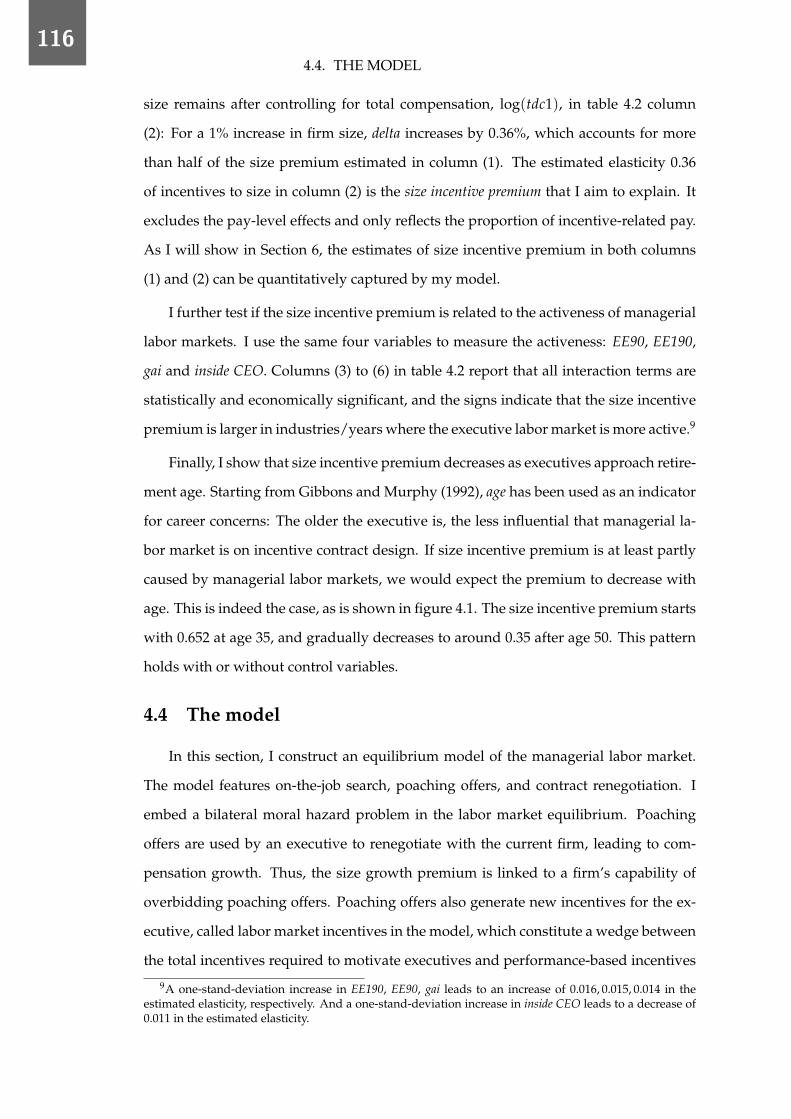
1164.4. THE MODEL
size remains after controlling for total compensation, log(tdc1), in table 4.2 column
(2): For a 1% increase in firm size, delta increases by 0.36%, which accounts for more
than half of the size premium estimated in column (1). The estimated elasticity 0.36
of incentives to size in column (2) is the size incentive premium that I aim to explain. It
excludes the pay-level effects and only reflects the proportion of incentive-related pay.
As I will show in Section 6, the estimates of size incentive premium in both columns
(1) and (2) can be quantitatively captured by my model.
I further test if the size incentive premium is related to the activeness of managerial
labor markets. I use the same four variables to measure the activeness: EE90, EE190,
gai and inside CEO. Columns (3) to (6) in table 4.2 report that all interaction terms are
statistically and economically significant, and the signs indicate that the size incentive
premium is larger in industries/years where the executive labor market is more active.9
Finally, I show that size incentive premium decreases as executives approach retire-
ment age. Starting from Gibbons and Murphy (1992), age has been used as an indicator
for career concerns: The older the executive is, the less influential that managerial la-
bor market is on incentive contract design. If size incentive premium is at least partly
caused by managerial labor markets, we would expect the premium to decrease with
age. This is indeed the case, as is shown in figure 4.1. The size incentive premium starts
with 0.652 at age 35, and gradually decreases to around 0.35 after age 50. This pattern
holds with or without control variables.
4.4 The model
In this section, I construct an equilibrium model of the managerial labor market.
The model features on-the-job search, poaching offers, and contract renegotiation. I
embed a bilateral moral hazard problem in the labor market equilibrium. Poaching
offers are used by an executive to renegotiate with the current firm, leading to com-
pensation growth. Thus, the size growth premium is linked to a firm’s capability of
overbidding poaching offers. Poaching offers also generate new incentives for the ex-
ecutive, called labor market incentives in the model, which constitute a wedge between
the total incentives required to motivate executives and performance-based incentives
9A one-stand-deviation increase in EE190, EE90, gai leads to an increase of 0.016, 0.015, 0.014 in theestimated elasticity, respectively. And a one-stand-deviation increase in inside CEO leads to a decrease of0.011 in the estimated elasticity.

CHAPTER 4. LABOR MARKET INCENTIVES
117
35 40 45 50 55 60 65age
0.3
0.4
0.5
0.6
0.7
0.8siz
e pr
emiu
m
Figure 4.1: Size premium in performance-based incentives decreases with age
Note: The figure depicts the size premium in performance-based incentives at each age from 35 to 65.Each point is one estimated coefficient of the interaction term between one age dummy and log(firmsize) in the following regression,
log(delta)it = Φ′age dummiesit × log(firm size)it + Ψ′Xit + εit,
where i denotes an executive, t denotes the fiscal year, age dummies is a set of 31 dummies for each agefrom 35 to 65, firm size is measured by market capitalization by the end of the fiscal year, calculatedby a firm’s common shares outstanding times the close price by fiscal year, X denotes a vector ofcontrol variables including a constant term. I control for total compensation log(tdc1) and dummiesof executive tenure, age, and fiscal year time industry. A 95% confidence interval is plotted using thestandard error clustered on firm times fiscal year. The full regression result is provided in AppendixB.
provided by firms. Thus, the size incentive premium is also linked to labor market
incentives. I now formally introduce the model.
4.4.1 Ingredients
Agents There is a fixed measure of individuals: They are either employed as exec-
utives or not hired as executives but are looking for executive jobs. I call the latter
“executive candidates”. Individuals die with some probability. Once an individual
dies, a new-born enters the economy. Individuals want to maximize expected lifetime
utility,
E0Σ∞t=0(β× (1− η))t(u(wt)− c(et)),
where β ∈ (0, 1) is the discount factor, η ∈ (0, 1) is the death probability, utility of
consumption u : R → R is increasing and concave and c(·) is the dis-utility of effort.
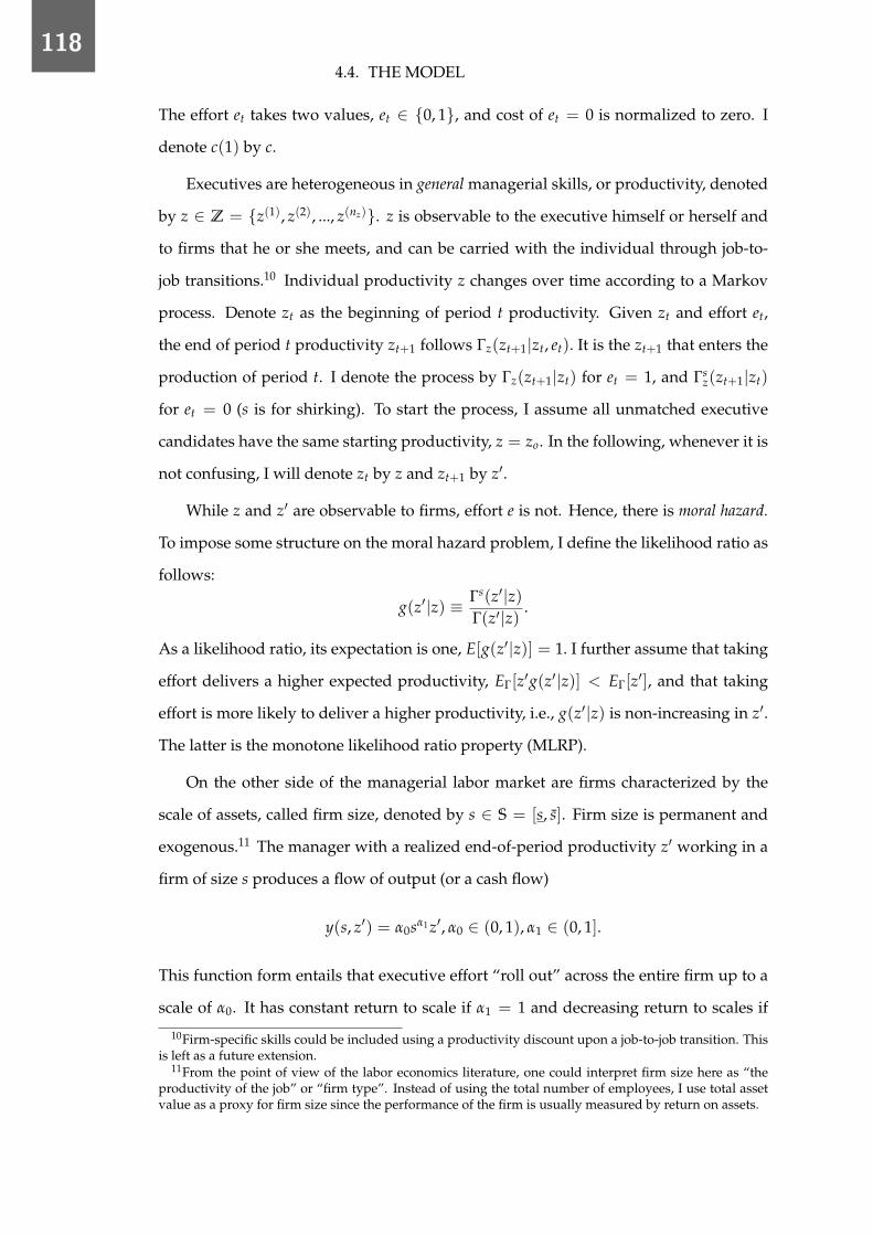
1184.4. THE MODEL
The effort et takes two values, et ∈ {0, 1}, and cost of et = 0 is normalized to zero. I
denote c(1) by c.
Executives are heterogeneous in general managerial skills, or productivity, denoted
by z ∈ Z = {z(1), z(2), ..., z(nz)}. z is observable to the executive himself or herself and
to firms that he or she meets, and can be carried with the individual through job-to-
job transitions.10 Individual productivity z changes over time according to a Markov
process. Denote zt as the beginning of period t productivity. Given zt and effort et,
the end of period t productivity zt+1 follows Γz(zt+1|zt, et). It is the zt+1 that enters the
production of period t. I denote the process by Γz(zt+1|zt) for et = 1, and Γsz(zt+1|zt)
for et = 0 (s is for shirking). To start the process, I assume all unmatched executive
candidates have the same starting productivity, z = zo. In the following, whenever it is
not confusing, I will denote zt by z and zt+1 by z′.
While z and z′ are observable to firms, effort e is not. Hence, there is moral hazard.
To impose some structure on the moral hazard problem, I define the likelihood ratio as
follows:
g(z′|z) ≡ Γs(z′|z)Γ(z′|z) .
As a likelihood ratio, its expectation is one, E[g(z′|z)] = 1. I further assume that taking
effort delivers a higher expected productivity, EΓ[z′g(z′|z)] < EΓ[z′], and that taking
effort is more likely to deliver a higher productivity, i.e., g(z′|z) is non-increasing in z′.
The latter is the monotone likelihood ratio property (MLRP).
On the other side of the managerial labor market are firms characterized by the
scale of assets, called firm size, denoted by s ∈ S = [s, s]. Firm size is permanent and
exogenous.11 The manager with a realized end-of-period productivity z′ working in a
firm of size s produces a flow of output (or a cash flow)
y(s, z′) = α0sα1 z′, α0 ∈ (0, 1), α1 ∈ (0, 1].
This function form entails that executive effort “roll out” across the entire firm up to a
scale of α0. It has constant return to scale if α1 = 1 and decreasing return to scales if
10Firm-specific skills could be included using a productivity discount upon a job-to-job transition. Thisis left as a future extension.
11From the point of view of the labor economics literature, one could interpret firm size here as “theproductivity of the job” or “firm type”. Instead of using the total number of employees, I use total assetvalue as a proxy for firm size since the performance of the firm is usually measured by return on assets.

CHAPTER 4. LABOR MARKET INCENTIVES
119
α1 < 1.12
Managerial labor market The managerial labor market is search-frictional. Execu-
tives and firms are imperfectly informed about executive types and location of firms.
The search friction precludes the optimal assignments assumed in Gabaix and Landier
(2008). Agents are only informed about each other’s types when they meet. Search is
random; executives and executive candidates all sample from the same, exogenous job
offer distribution F(s). Unmatched candidates meet firms with probability λ0, while
on-the-job executives meet firms with probability λ1. I treat these parameters as exoge-
nous.13
When a candidate meets a firm, they bargain on a contract. Suppose the continua-
tion value of an unmatched executive candidate is W0. Then, the firm ultimately offers
a contract with a continuation value of W0, for there is no other credible threat. The
individual then enters the next period as an employed executive.
When an on-the-job executive meets an outside firm, a compensation renegotiation
is triggered. Otherwise, the executive has an interest in transiting to the outside firm. I
allow the incumbent firm to respond to outside offers: A sequential auction is played
between the executive and both firms as in Postel-Vinay and Robin (2002). If the poach-
ing firm is larger, the executive moves to the alternative firm, for the poaching firm can
always pay more than the current one can match. Alternatively, if the poaching firm is
smaller, then the executive may use the outside offer to negotiate up his/her compen-
sation. This sequential auction mechanism characterizes labor market competition in
this paper.
Timing Time is discrete, indexed by t, and continues forever. The period of an exec-
utive candidate is simple — he or she is matched to a firm with some probability and
starts with a contract of continuation value W0. An on-the-job executive enters a pe-
riod with beginning-of-period productivity z and current firm of size s. The timing is
12There has been some discussion in this literature on the appropriate production function of execu-tives, see e.g., Edmans et al. (2017). Take s as firm size and z as the executive’s per unit contribution toshareholder values. An additive production function such as y(s, z) = s + z implies that the effect of exec-utives on firm value is independent of firm size. This specification is appropriate for perk consumption.A multiplicative production function such as y(s, z) = sz is appropriate for executives’ actions that canroll out across the entire firm and thus have a greater effect in a larger company. The latter is the functionform adopted here.
13So we are in a “partial” equilibrium, in contrast to the “general” equilibrium where the labor markettightness is determined in the equilibrium.

1204.4. THE MODEL
shown in figure 4.2.
Figure 4.2: Timing
1. Compensation: The current firm of size s gives a compensation of w for this
period, in accordance with the contract value that are promised before.
2. Production: The executive chooses an effort level, e ∈ {0, 1} and his/her produc-
tivity z′ is then realized according to Γ(z′|z, e) where z is the beginning-of-period
productivity level. The firm only observes the output y(z′, s), which is a func-
tion of productivity z′ and firm size s, not the effort e. This is the moral hazard
problem. z′ becomes the beginning-of-period productivity of the next period.
3. Labor market: With probability η the executive dies; otherwise, with probability
λ1, a job offer from a firm with size s ∼ F(s) arrives. The renegotiation game is
triggered. The executive may stay in the current firm and receive higher compen-
sation, or transit to the poaching firm. The value of the contract to the executive
is determined by a sequential auction between the current and poaching firms.
The compensation w, effort choice e and job-to-job transitions in future periods are
stipulated in the contract between the firm and the executive, defined on a proper state
of the world, which we now turn to.
Contractual environment A contract defines the transfers and actions of the executive
and the firm in a matched pair for all future histories, where a history summarizes the
past states of the world. I define a history as follows. Call ht = (z′t, st) the state of the
world by the end of period t, where z′t is the realized productivity by the end of t and
st is the size of a poaching firm. Let s = so if there is no poaching firm. The history
of productivity and the poaching firm up to period t, denoted by ht = (h1, h2, .., ht), is
common knowledge to the executive and the firm, and is fully contractible.

CHAPTER 4. LABOR MARKET INCENTIVES
121
The two elements included in the history — productivity and poaching firm —
correspond to the frictions I have in the contracting problem, namely moral hazard and
search frictions. First, while productivity is included in the history and is contractible,
the executive’s effort is not and needs to be induced by incentives. Hence, an incentive
compatibility constraint is required. Second, by including poaching firms in the history,
I allow a contract to stipulate whether and how to counter poaching offers. That is,
competing for executives is involved in the contracting problem.
Countering outside offers is optimal (or subgame perfect in game terminology);
it is, therefore, necessary to allow limited commitment for both sides — to terminate
the contract when the surplus is negative. Firms cannot commit to the relationship if
the profits are negative. When the outside offer comes from a larger firm, the firm’s
participation constraint binds, and the match separates. Likewise, executives cannot
commit to the match if the current firm cannot provide more than the outside value, be
the unmatched value W0 or the offer value of a poaching firm. In the former case, the
executive is fired by the board. In the latter case, the executive transits to the poaching
firm.
Given the information structure, I define a feasible contract as a plan that defines
compensation wt(ht−1), a recommended effort choice et(ht−1) and whether to terminate
the contract It(ht) in every future history, represented by
{et(ht−1), wt(ht−1), It(ht)}∞t=0,
that satisfies the participation constraints of both sides and an incentive compatibility
constraint.
To further simplify, I impose two assumptions. First, I assume taking effort, e = 1,
is optimal. This assumption is consistent with Gayle et al. (2015) and in accordance with
the fact that almost all executives in my data are provided with an incentive package.
Secondly, I assume a reasonable support of productivity z such that the profits of a firm
are always non-negative at the unmatched value W0. As a result, firing is excluded,
and It(ht) = 1 is equivalent to a job-to-job transition.14
14If I allow a large domain of z such that for some z the profit is negative at promised continuation valueW0, then firing happens. This is left as an extension in the future.

1224.4. THE MODEL
A simplified contract state space To recursively write up the contracting problem, I
use the executive’s beginning-of-period expected utility, denoted by V, as a co-state
variable to summarize the history of productivities and outside offers. A dynamic
contract, defined recursively, is
σ ≡ {e(V), w(V), W(z′, s, V)|z′ ∈ Z, s′ ∈ S and V ∈ Φ},
where e is the effort level suggested by the contract (optimal level is assumed to be
1), w is the compensation, W is the promised value given for a given state (z′, s), and
Φ is the set of feasible and incentive compatible expected utilities that can be derived
following Abreu et al. (1990).15
4.4.2 Optimal contracting problem
In this section, I first characterize the participation constraints derived from the
sequential auction, then I describe the contracting problem.
Sequential auction Here I illustrate the sequential auction using value functions.16 Let
Π(z, s, V) denote the discounted profit of a firm with size s, executive of beginning-of-
period productivity z and a promised value to the executive V. The maximum bidding
values W(z, s) are defined by
Π(z, s, W) = 0.
The firm would rather fire the executive (normalizing the vacancy value to 0) if he or
she demands a value higher than W. I let W(z, so) ≡ W0, meaning that when there is
no outside offer, the executive’s outside value is simply W0. I call W(z, s) the bidding
frontier to highlight that it is a function (frontier) in terms of z and s.
The sequential auction works as follows. When the executive from a firm of size
s (hereafter firm s) meets a poaching firm of size s (hereafter firm s), both firms enter
a Bertrand competition won by the larger one. Since it is willing to extract a positive
marginal profit out of every match, the best firm s can do is to provide a promised
15Promised utilities as co-states have been used extensively in models with incentive or participationconstraints. Among others, Phelan and Townsend (1991) studied a model of risk-sharing with incentiveconstraints, Kocherlakota (1996) analyzed the risk-sharing model with two-sided limited commitment,Hopenhayn and Nicolini (1997) studied a model of unemployment insurance, and Alvarez and Jermann(2000) studied a decentralized version of the above risk-sharing model with debt constraints.
16What distinguishes this model from the original sequential auction framework is that here the wageis not flat. Firms compete on a stream of wages contingent on all possible future histories. At each period,the contract defines a wage on each state (z, s).

CHAPTER 4. LABOR MARKET INCENTIVES
123
utility W(z′, s). When s > s, the executive moves to a potentially better match with
firm s, if the latter offers at least the W(z′, s). Any less generous offer on the part of
firm s is successfully countered by firm s. If s is smaller than s, then W(z′, s) > W(z′, s),
in which case firm s will never raise its offer up to this level. Rather, the executive will
stay at his or her current firm, and be promoted to the continuation value W(z′, s) that
makes him/her indifferent between staying and joining firm s.
The above argument defines outside values of the executive contingent on the state
(z′, s),
W(z′, s) ≥ min{W(z′, s), W(z′, s)}.
This is the participation constraint of the executive in a contracting problem.
The contracting problem In designing the contract, the firm chooses a wage w and
a set of promised values W(z′, s) depending on the state (z′, s). For ease of notation, I
denote an effective discount factor, β = β(1− η), and write the mixture distribution of
outside offers as follows:
F(s) = I(s = so)(1− λ1) + I(s 6= so)λ1F(s).
The expected profit of the firm can be expressed recursively as
Π(z, s, V) = maxw,W(z′,s)
∑z′∈Z
[y(s, z′)− w + β ∑
s≤sΠ(z′, s, W(z′, s))F(s)
]Γ(z′|z). (BE-F)
subject to the promise-keeping constraint,
V =u(w)− c + β ∑z′∈Z
∑s∈S
W(z′, s)F(s)Γ(z′|z), (PKC)
the incentive compatibility constraint,
β ∑z′∈Z
∑s∈S
W(z′, s)F(s)(1− g(z, z′))Γ(z′|z) ≥ c. (IC)
and the participation constraints of the executive and the firm,
W(z′, s) ≥ min{W(z′, s), W(z′, s)} (PC-E)
W(z′, s) ≤W(z′, s). (PC-F)
The objective function (Bellman Equation of the Firm, BE-F) includes a flow profit
of y(s, z′)−w, plus the continuation value taking into account that the match may sep-

1244.4. THE MODEL
arate either because the executive dies, which happens with probability η, or transits
to another firm, which happens with probability ∑s>s F(s).
The promise-keeping constraint (PKC) makes sure that the choices of the firm honor
the promise made in previous periods to deliver a value V to the executive, and the
promised value V contains all the relevant information in the history. The right-hand
side of the constraint is the lifetime utility of the executive given the choices made by
the firm. (PKC) is also the Bellman equation of an executive with state (z, s, V).
The incentive compatibility constraint (IC) differentiates itself from the promise-
keeping constraint by the term 1 − g(z′|z). It asserts that the continuation value of
effort is higher than no effort. This creates incentives for the executive to pursue the
shareholders’ interests rather than his or her own.
Finally, the participation constraints are stated in (PC-E) and (PC-F). The firm com-
mits to the relationship as long as the promised value is no more than W(z′, s). The
sequential auction pins down the outside value of the executive, which is the minimum
of bidding frontier of the poaching firm, W(z′, s), and of the current firm, W(z′, s).
4.4.3 Equilibrium definition
Before turning to the characterization of the optimal contract, I define the equilib-
rium. An equilibrium is an executive unemployment value W0, a value function of
employed executives W that satisfies (PKC), a profit function of firms Π and an opti-
mal contract policy σ = {w, e, W(z′, s)} for z′ ∈ Z and s ∈ S that solves the contracting
problem (BE-F) with associated constraints (PKC), (IC), (PC-E) and (PC-F), a stochastic
process of executive productivity Γ that follows the optimal effort choice, and a distri-
bution of executives across employment states evolving according to flow equations.
The proof of the existence of the equilibrium is an exercise applying Schauder’s fixed
point theorem, as shown by Menzio and Shi (2010) and Lentz (2014). Here I base my
results on the existence of the equilibrium without giving the proof.
4.4.4 Contract characterization
In this section, I derive a characterization of the optimal contract. The characteriza-
tion builds on and extends the dynamic limited commitment literature, pioneered by
Thomas and Worrall (1988) and Kocherlakota (1996), the dynamic moral hazard liter-

CHAPTER 4. LABOR MARKET INCENTIVES
125
ature, pioneered by Spear and Srivastava (1987), and related literature in labor search
such as Lentz (2014).
Proposition 4.1. Π(z, s, V) is continuous differentiable, decreasing and concave in V, and
increasing in z and s. An optimal contract evolves according to the following updating rule.
Given the beginning-of-period state (z, s, V), the current period compensation is given by w∗,
∂Π(z, s, V)
∂V= − 1
u′(w∗), (4.1)
and the continuation value W∗(z′, s) follows
W∗(z′, s) =
W(z′, s) if W(z′, s) ≥W(z′, s) or W(z′) > W(z′, s)
W(z′, s) if W(z′, s) > W(z′, s) > W i(z′)
W(z′) if W(z′, s) ≥W i(z′) ≥W(z′, s)
(4.2)
where W(z′) satisfies
∂Π(z′, s, W(z′))∂W(z′)
− ∂Π(z, s, V)
∂V= −µ(1− g(z, z′)). (4.3)
Proof. The properties of Π(z, s, V) follow immediately from the proof of Lentz (2014).To characterize the optimal contract, I assign Lagrangian multipliers λ to (PKC), µ to(IC), βµ0(z′, s) to (PC-E) and βµ1(z′, s) to (PC-F). The first order condition w.r.t w gives
u′(w) =1λ
,
and the envelop theorem gives
−∂Π(z, s, V)
∂V= λ.
They together give (4.1). Participation constraints (PC-E) and (PC-F) can be simplified.If W(z′, s) ≥ W(z′, s), we have W(z; , s) = W(z′, s). This is the first case in line 1 of(4.2). If W(z′, s) ≥ W(z′, s), the participation constraints become W(z′, s) ≤ W(z; , s) ≤W(z′, s). Use this to derive the first order condition w.r.t W(z′, s):
−∂Π(z′, s, W(z′, s))∂W(z′, s)
= λ + µ(1− g(z, z′)) + µ0(z′, s)− µ1(z′, s).
If µ0(z′, s) = µ1(z′, s) = 0, W(z′, s) = W(z′) defined by (4.3). This is the case in line 3of (4.2). If µ0(z′, s) > µ1(z′, s) = 0, W(z′, s) = W(z′, s). This is the case in line 2 of (4.2).Finally, if µ1(z′, s) > µ0(z′, s) = 0, W(z′, s) = W(z′, s). This is the second condition inline 1 of (4.2).
Proposition 4.1 states that, if one abstracts from the participation constraints, an

1264.4. THE MODEL
optimal contract inherits the essential properties of the classical infinite repeated moral
hazard model (Spear and Srivastava 1987). Equation (4.1) states that the current period
compensation w∗ is directly linked to the promised continuation utility V, by equat-
ing the principal’s and agent’s marginal rates of substitution between the present and
future compensation. Equation (4.3) says, abstract from participation constraints, the
continuation utility W(z′) only changes to induce the executive effort. In the extreme
case that the IC constraint is not binding (µ = 0, µ is the multiplier of the IC constraint),
W(z′) = V remains constant. Thus, the pay is also constant over time. Generally speak-
ing, a higher V induces a higher W(z′). That is, an optimal dynamic contract has some
memory.
When outside offers are realized such that the participation constraint is binding,
the contract is no longer dependent on history, and the continuation value depends
only on the current state. This is what Kocherlakota (1996) calls amnesia. More precisely,
when the outside firm is larger s ≥ s, the continuation value equals the bidding frontier
of the current firm W(z′, s) = W(z′, s); when the outside firm is smaller, s < s, the
continuation value depends on whether the bidding frontier of the outside firm W(z′, s)
can improve upon W(z′).
Even when the participation constraint is binding, amnesia of the optimal contract
is not “complete” — although W does not depend on the previously promised utility
V, it does depend on the executive’s productivity z′, which is stochastically determined
by past effort. Therefore, the boundaries of participation constraints carry the memory
of the prior effort choice. This is where the incentives from the labor market come into
effect.
4.4.5 Explaining the size pay-growth premium
With the characterization of the optimal contract, we are ready to explain the size
premium in pay-growth and incentives. I start by defining two sets of poaching firms
s: larger or smaller than the current firm.
M1(s) ≡ {s ∈ S|s > s},
M2(z, s, W) ≡ {s ∈ S|W(z, s) > W(z, s), W < W(z, s)}.

CHAPTER 4. LABOR MARKET INCENTIVES
127
Given a poaching firm that belongs to the setM1, the executive will transit to such a
firm and receive the full surplus of his or her previous job W(z, s). Given a poaching
firm in M2, the executive will stay in the current firm but use the outside offer to
renegotiate up to W(z, s). Any poaching firm that is not inM1 orM2 is not competitive
in the sense that it cannot be used to negotiate compensation with the incumbent firm.
Accordingly, the Bellman equation of executives can be written as:17
V = u(w)− c + β ∑z′
[λ1 ∑
s′∈M1
F(s′)W(z′, s) + λ1 ∑s′∈M2
F(s′)W(z′, s′)
+(
1− λ1 ∑s′∈M1∪M2
F(s′))
W(z′)
]Γ(z′|z), (PKC’)
(PKC’) shows that compensation grows mainly in two cases: i) There is a poaching firm
from set M2 and total compensation increases without a job turnover; ii) There is a
poaching firm from setM1 and total compensation grows upon a job-to-job transition.
The firm-size pay-growth premium observed in the data refers to the growth in the
former case. In the latter case, compensation may also decrease if an executive is willing
to make sacrifices on his or her current pay for the sake of higher pay in the future.18
To understand the firm-size pay-growth premium, consider two executives from a
small firm s1 and a large firm s2, s2 > s1. For simplicity, suppose they have the same
continuation value W(z′). Since the firm s2 has a higher output and is more capable
of overbidding outside offers, the corresponding setM2 is larger. That is, there exist
poaching firms with a size between s1 and s2 such that the firm s2 can overbid and
retain the executive with compensation growth while the firm s1 cannot overbid and
consequently lose the executive. Therefore, the total pay increases faster in the larger
firm s2.17We can similarly rewrite the Bellman equations of firms using the optimal continuation value, and
this equation is consistent with Postel-Vinay and Robin (2002):
Π(z, s, V) = maxw,W(z′)
∑z′
[y(s)z′ − w + β
(λ1 ∑
s′∈M2
F(s′)Π1(z′, s, W(z′, s′)
+(
1− λ1 ∑s′∈M1∪M2
F(s′))
Π1(z′, s, W(z′))
)]Γ(z′|z). (BE-F’)
18Where compensation information is available in both the original and target firms, it would be in-teresting to examine whether there is also a firm-size compensation-growth premium in job-to-job transi-tions. This is, however, not possible with the current dataset.

1284.4. THE MODEL
4.4.6 Explaining the size incentive premium
To explain the firm-size incentive premium, I define “performance-based incen-
tives” and “labor market incentives” in the model. Using these definitions to rewrite
the IC constraint, I then show that the two sources of incentives substitute for each
other given a constant effort cost. Finally, I explain that labor market incentives de-
crease with firm size. Thus, performance-based incentives increase with firm size.
I first define an “incentive operator”, I(·), which calculates the incentives an exec-
utive receives from a continuation utility scheme:
I(
W(z′))≡∫
z′W(z′)(1− g(z, z′))Γ(z′|z).
I then rewrite the IC constraint using the incentive operator:
λ1
∫s∈M1
dF(s)I(
W(z′, s))+ λ1
∫s∈M2
I(
W(z′, s))
F(s)
+(
1− λ1 ∑s∈M1∪M2
F(s))I(
W(z′))≥ c/β, (IC′)
It is clear from the left-hand-side of IC′ that the incentives comprise: i) incentives
brought by larger firms inM1 (the first item); ii) incentives brought by smaller firms
inM2 (the second item); iii) incentives in performance-related pay when there are no
poaching firms fromM1 orM2 (the third item).
The incentives when there are no competitive poaching offers are the performance-
based incentives, denoted by Ξp:
Ξp
(W(z′)
)≡(
1− λ1 ∑M1∪M2
F(s′))I(
W(z′))
, (4.4)
and the incentives from poaching offers are the labor market incentives, denoted by Ξm:
Ξm
(s, W(z′)
)≡ λ1
∫s∈M1
dF(s)I(
W(z′, s))+ λ1
∫s∈M2
I(
W(z′, s))
F(s). (4.5)
Ξm would be zero if there were no poaching offers.
Because of labor market incentives, the need for performance-based incentives is
less. Intuitively, firms appreciate higher productivities and are willing to bid higher
for a more productive executive. The sequential auction in the model therefore begets
labor market incentives for executive effort: If working hard today is not only an input
into current production but also an investment in the (inalienable and transferable)

CHAPTER 4. LABOR MARKET INCENTIVES
129
human capital, then it is intuitive that the objectives of the firm and of the executive
become better aligned and the need for short-term compensation incentives decreases.
Mathematically, Ξm is an expectation of incentives from all possible poaching of-
fers. When the poaching firm is larger than the current firm, the incentives are from
the bidding frontier of the current firm. When the poaching firm is smaller than the
current firm, the incentives are from the bidding frontier of the poaching firm.
The magnitude of Ξm is determined by current firm size s and the promised con-
tinuation value W(z′). In particular, firm size s enters Ξm via bidding frontiers. That is,
Ξm depends on s even though the moral hazard problem fundamentally does not. On
the other hand, W(z′) determines the lower bound of setM2. The larger the promised
continuation value W(z′), the less likely a poaching firm can be used to renegotiate
with the current firm, and the lower the labor market incentives.
Based on this, there is a simple “job ladder” explanation for the size premium when
comparing executives of different pay levels. Such an incentive premium is reported
in column (1) in table 4.2. Since executives of larger firms tend to have higher total
compensation, the corresponding continuation values are larger; they are thus higher
on the job ladder. Accordingly, the chance of encountering a competitive poaching of-
fer that beats the current value is smaller. Hence, labor market incentives are lower.
As a result, executives in larger firms require more incentives in performance-related
pay.19As we will see in the following section, this “job ladder” argument also applies
to explaining the size incentive premium among executives with the same total com-
pensation.
Labor market incentives decrease with firm size Now I compare labor market in-
centives for executives who have the same total compensation but come from firms of
different size. I show that when there is enough concavity in the utility function, labor
market incentives decrease with firm size. Therefore, larger firms need to provide more
performance-based incentives. This explains the firm-size incentive premium.
Consider two executives from firms s1 and s2, s1 < s2. The executives have the
same total compensation. Figure 4.3 illustrates the possible poaching firm sizes for
the two executives and the associated incentives. The poaching firm size ranges from
19This is an alternative explanation in addition to the current explanations based on moral hazard(Gayle and Miller, 2009) and on multiplicative utility (Edmans et al., 2009).

1304.4. THE MODEL
s
s1
s
s2
slb2
M1(s1)
slb1
poaching firms and
∫s∈M1(s1)
I[W (z′, s1)]dF (s)
∫s∈M2(s1,w)
I[W (z′, s)]dF (s)
M2(s1, w)
M1(s2)∫s∈M1(s2)
I[W (z′, s2)]dF (s)
M2(s2, w)∫s∈M2(s2,w)
I[W (z′, s)]dF (s)
market-based incentives for s1
poaching firms and
market-based incentives for s2
Figure 4.3: Compare labor market incentives
Note: The figure illustrates labor market incentives for executives with the same compensation w fromfirms of size s1 and s2. The vertical axis labels the size of poaching firms [s, s]. slb
1 is the lower boundof setM2(s1, w) and slb
2 is the lower bound of setM2(s2, w). The labor market incentives of s1 and s2are on the left and right of the vertical axis, respectively. The notation for each interval is followed bythe value of incentives from poaching firms of that interval.
s to s. I denote the lower bound ofM2 for firms s1 and s2 by slb1 and slb
2 , respectively.
Notice that slb2 > slb
1 because they are determined by lifetime utilities rather than current
period compensation. Although the two executives have the same total compensation,
the one in s2 has higher lifetime utility. The left side of the axis depicts setsM1, M2
and corresponding labor market incentives in the two sets for the executive in s1. The
right side of the axis depicts the counterparts for s2. Taking the difference between

CHAPTER 4. LABOR MARKET INCENTIVES
131
Ξm(s2) and Ξm(s1), we have
Ξm(s2)− Ξm(s1) =−∫ slb
2
slb1
dF(s)I(W(z′, s))
+∫ s
s2
dF(s)(I(W(z′, s2)− I(W(z′, s1)
)+∫ s2
s1
(I(W(z′, s)− I(W(z′, s1)
)dF(s). (4.6)
Their labor market incentives are different in two respects. First, with poaching
firms in [slb1 , slb
2 ], the executive in s1 receives an incentive of∫ slb
2slb
1dF(s)I(W(z′, s)), while
the executive in s2 has no incentive from the labor market. This is the first item in (4.6),
and it corresponds to the job ladder argument previously mentioned — since slb2 > slb
1 ,
the executive in s2 is less likely to receive a competitive outside offer, and labor market
incentives are lower.
Second, for poaching firms in the range of [s1, s], labor market incentives for firms
s1 and s2 are drawn on different bidding frontiers, which correspond to the second and
third items in (4.6). With poaching firms in this range, the bidding frontier for the ex-
ecutive of firm s1 is always W(z′, s1), since any poaching firm larger than s1 can bid
just W(z′, s1) to attract the executive. In contrast, the bidding frontiers for the exec-
utive in firm s2 are either W(z′, s2) or W(z′, s) with s > s1, both of which are larger
than W(z′, s1).20 Consequently, the certainty equivalent of the executive in s2 is higher.
By diminishing marginal utility, the incentives from these higher bidding frontiers are
lower:
I(
W(z′, s1))> I
(W(z′, s)
)for s > s1.
This is a wealth effect of poaching offers — a wealthier executive is harder to incen-
tivize. This wealth effect holds as long as the utility function is sufficiently concave. In
the following, I give a sufficient condition under the restriction that the utility function
is of the CRRA form and effort cost c is equal to a particular value.
Proposition 4.2 (Labor market incentives and firm size). Suppose the executives’ utility is
of the CRRA form, and the cost of effort c = c(s), then I(
W(z′, s))
decreases in s if
σ > 1 +s1−α1
α1ψ′(s), (4.7)
20W(z′, s) is strictly increasing in s.

1324.4. THE MODEL
where ψ(s) is a function of s that is positive and increasing in s and
c(s) ≡ β ∑z′∈Z
W(z′, s)(1− g(z′|z))Γ(z′|z).
Proof. See the Appendix.
To understand the proposition, first notice that I(
W(z′, s))
is simply a weight sum
of ∆W(z′,s)∆z′ over the domain of z′ — the steeper W(z′, s) with respect to z′, the higher the
incentives to induce effort. So it would be sufficient to show that ∆W(z′,s)∆z′ decreases in s
under the stated condition. To proceed, it follows that
∆W(z, s)∆z
= −∆Π(z, s, W)/∆z∆Π(z, s, W)/W
=α× s
1/u′(w), (4.8)
where w is the optimal compensation for the current period, corresponding to a promis-
ing continuation value W. The first equality follows from an implicit differentiation. In
the second equality,
∆Π(z, s, W)/∆z = α× s
because keeping the promised value, all increasing output is accrued to the company.
In particular, α is α multiplied by a factor that adjusts for the possibility that the execu-
tive will leave the firm and the job is destructed. On the denominator,
∆Π(z, s, W)/W = −1/u′(w)
follows directly from condition (4.1) in Proposition 4.1.
There are two opposing effects of s involved in (4.8). On the one hand, the maxi-
mum value that larger firms are able to bid changes more with respect to z due to the
multiplicative production function. This will generate more labor market incentives,
and it is reflected in the numerator of (4.8). On the other hand, the incentives in terms
of utilities can actually be lower because the marginal utility for extra returns from
the executive labor market is lower now (w increases in s making u′(w) lower). This
is reflected in the denominator of (4.8). The second force dominates when the utility
function has enough concavity, as stated in the proposition.
The requirement stated in (4.7) is consistent with the literature in this context. The
existing studies usually estimate or calibrate a higher σ value. For example, a careful

CHAPTER 4. LABOR MARKET INCENTIVES
133
calibration study on CEO incentive pay by Hall and Murphy (2000) uses σ between 2
and 3. Calibration exercises on CEO incentive compensation convexity starting from
Dittmann and Maug (2007) are based on σ > 1. Using an employer-employee matched
data from Sweden for the general labor market, Lamadon (2016) estimates that σ =
1.68. Numerically, I find the right-hand side of (4.7) is approximately equal to one in
the parameter space explored in my estimation.
Back to the firm-size incentive premium. If (4.7) is satisfied, and given (4.6), the
labor market incentives Ξm are lower for the executive in firm s2. Since the effort cost is
the same for both executives, the executive in the larger firm s2 demands more incen-
tives from the performance-related pay. This explains the firm-size incentive premium.
4.5 Empirical evidence
To quantitatively evaluate the model, I use data on executives employed in U.S.
publicly listed firms. Close scrutiny of the managerial labor market allows me to put
together a rich array of data from various sources. Specifically, I assemble a new dataset
on job turnovers from BoardEX, and merge the job turnover data with two sets of stan-
dard data, the executive compensation from ExecuComp, and firm-level information
from CompuStat. In the following, I provide a brief description of the relevant data
features. In particular, I examine executives’ job-to-job transitions, and whether they
climb the job ladder towards larger firms. These are the key features of the managerial
labor market in the model. Additionally, I examine whether the job-to-job transition
rate decreases with firm size as predicted by the model.
4.5.1 Data
The empirical analysis and estimation mainly rely on the ExecuComp database,
which provides rich information on executive compensation of the top five to eight
executives in companies included in the S&P 500, MidCap and SmallCap indices for
the period of 1992 to 2016. The accounting information from CompuStat and stock re-
turns from CRSP are merged with ExecuComp. The dataset provided by Coles et al.
(2006) and Coles et al. (2013) contains performance-based incentives delta calculated
based on ExecuComp. To collect job turnover information, I extract the full employ-
ment histories of executives from the BoardEX database, and supplement them with

1344.5. EMPIRICAL EVIDENCE
Table 4.3: Summary statistics
Variable N mean sd p25 p50 p75age 218,168 51.04 6.96 46 51 56male 218,168 0.936 0.244 1 1 1CEO 218,168 0.184 0.387 0 0 0CFO 218,168 0.096 0.295 0 0 0director 218,168 0.339 0.473 0 0 1interlock 218,168 0.013 0.112 0 0 0tenure 218,168 4.71 3.793 2 4 6tdc1 (in $000s) 198,673 2,555.527 5,454.153 632.164 1,270.806 2,690.385delta (in $000s) 146,790 322.518 4,736.982 16.966 50.634 154.411mkcap (in $000, 000) 212,271 7,997.377 25,810.758 598.919 1,622.236 5,169.379at (in $000, 000) 216,384 15,594.888 98,653.077 542.863 1,796.467 6,570.342sales (in $000, 000) 216,276 5,472.709 17,387.175 428.2 1,217.738 3,917.269profit 209,639 0.119 0.359 0.069 0.121 0.176annual return 211,067 0.181 0.802 -0.127 0.106 0.356mbr 183,565 1.669 2.21 0.811 1.198 1.913
Note: The table reports summary statistics for my sample, which covers named executive officersreported in ExecuComp over the period of 1992 to 2016. age is the executive’s age by the end ofthe fiscal year. Sample episodes with age lower than 35 or higher than 70 are dropped. Dummyvariables CEO, CFO, director and interlock indicate whether the executive served as a CEO, or a CFO, ora director, or is involved in the interlock relationship during the fiscal year, respectively. An interlockrelationship is described in the note of table 4.1. tenure (in years) counts the number of fiscal yearsthat an executive works as a named officer in a particular company. tdc1 is the total compensation,composed of the following: Salary, Bonus, Other Annual, Total Value of Restricted Stock Granted,Total Value of Stock Options Granted (using Black-Scholes), Long-Term Incentive Payouts, and AllOther Total. delta is the dollar change in wealth associated with a 1% change in the firms stock price (in$000s). mkcap (in millions) is the market capitalization of the company, calculated by csho (CommonShares Outstanding, in millions of shares) multiplied by prcc f (fiscal year end price). prcc f andcsho are reported in the Compustat Fundamentals Annual files. at (in millions) is the Total BookAssets as reported by the company. sales (in millions) is the Net Annual Sales as reported by thecompany. profit is the profitability, calculated by EBITDA/Assets. annual return is the annualized stockreturn which is compounded based on CRSP MSF (Monthly) returns. MSF returns have been adjustedfor splits, etc. mbr is the Market-to-Book Ratio, calculated by Market Value of Assets divided byTotal Book Assets. Market Value of Assets is calculated according to Market Value of Assets (MVA) =prcc f ∗ cshpri + dlc + dltt + pstkl − txditc. Variable definitions are also provided in the main text.

CHAPTER 4. LABOR MARKET INCENTIVES
135
the information from the LinkedIn and Bloomberg pages of a subset of executives.
My final sample comprises 35, 088 executives with age between 30 and 65.21 Of
these, 26, 972 episodes cover the full tenure of the executive from beginning to end.
The total number of executive-fiscal year observations in my sample is 218, 168. The
minimum number of firms covered in a given year is 1, 556 in 1992, and the maximum
is 2, 235 in 2007. All nominal quantities are converted into constant 2016 dollars using
a GDP deflator from the Bureau of Economic Analysis.
Here I describe the variables that are used in my analysis. Using information from
ExecuComp, I identify the gender and age for each executive, the tenure in the current
executive episode, whether he or she is a CEO, or CFO, or director of the board or is
involved in an interlock relationship during the fiscal year. Table 4.3 reports summary
statistics for my sample. More than ninety-three percent of the executives are males
and the average age is 51. The average length of an episode is 6.21 years. Among all
executive-year observations, 18.4% are CEO spells and 9.6% are CFO spells.
In terms of the compensation information, tdc1 is the total compensation including
salary, bonus, values of stock and options granted, etc. The total compensation has
an average of 2, 555, 527 dollars, with a 25th percentile of 632, 164 dollars and a 75th
percentile of 2, 690, 385 dollars. In terms of means, only 16.5% of the total compensa-
tion is fixed base salary; the rest is all incentive-related. Performance-based incentives
come not only from the total compensation each year, but also from the stocks and
options that are granted in previous years. The variable delta measures how strong
performance-based incentives are in firm-related wealth. It is defined by the dollar
change in wealth (in $000s in table 4.3) associated with a 1% change in the firms stock
price. The distribution of delta is right-skewed, with a mean of 323, 518 dollars, even
larger than its 75th percentile of 154, 411 dollars.
For the firm-side information, I use market capitalization mkcap, the market value
of a company’s outstanding shares, to measure the firm size. In some robustness checks
(not shown in the main text), I also use book value of assets at and sales to measure firm
size. They are in millions of dollars. I use operating profitability, denoted by profit, to
measure firm performance. Two alternative measures for firm performance are stock
21I select this age range because the managerial labor market is more relevant than for those passing theretirement age.

1364.5. EMPIRICAL EVIDENCE
market annualized return, denoted by annual return, and market-to-book ratio, denoted
by mbr.
The job turnover information comes from the BoardEX database.22BoardEX con-
tains details of each executive’s employment history, including start and end dates,
firm names and positions. It also has extra information on educational background,
social networks, etc. I merge the two databases using three sources of information: (1)
the executive’s first, middle and last names, (2) date of birth, and (3) working expe-
riences, i.e. in which years the executive worked in which firms. If all three aspects
are consistent, the executive is identified. For executives that cannot be identified in
BoardEX, I search for the respective LinkedIn and Bloomberg pages and manually col-
lect the available employment information. In this way, I am able to identify more than
93% of executives in ExecuComp, 32, 864 in total.
4.5.2 Job-to-job transitions
30 35 40 45 50 55 60 65 70 75Age (years)
0.00
0.01
0.02
0.03
0.04
0.05
0.06
0.07
0.08
Job-
to-J
ob T
rans
ition
Rat
e (%
)
Figure 4.4: Job-to-job transition rate over age
Note: The figure depicts estimated job-to-job transition rates over age with the 95% confidence interval. Ajob-to-job transition is defined as an executive leaving the current firm and starting to work in another firmwithin 190 days.
I define a job-to-job transition as an executive leaving his/her current firm and
starting to work in another within 190 days. Otherwise, the event is defined as an exit
22What is missing in the ExecuComp database is the information on executives’ employment history.For example, there is no information to identify whether the executive transits to another firm after thecurrent position in an S&P firm or whether he/she simply retires. Moreover, the start and end dates ofcurrent employment are not known.

CHAPTER 4. LABOR MARKET INCENTIVES
137
30 35 40 45 50 55 60 65 70 75Age (years)
0.02
0.04
0.06
0.08
0.10
0.12
0.14
Exit
Rat
e (%
)
Figure 4.5: Exit rate over age
Note: The figure depicts the estimated exit rates over age with the 95% confidence interval. A job exit isdefined as an executive leaving the current firm and not working in another firm within 190 days.
4 2 0 2 4 6 8 10Market Cap of the targer firm minus Market Cap of the original firm (dollar in billions)
0.0
0.1
0.2
0.3
0.4
0.5
0.6
Figure 4.6: Distribution of the change of firm size upon job-to-job transitions

1384.5. EMPIRICAL EVIDENCE
0.0 1.0 2.0 3.0 4.0 5.0 6.0 7.0 8.0 9.0 10.011.012.013.014.015.016.017.018.019.020.021.022.023.024.025.026.027.028.029.030.031.032.033.034.035.036.037.038.039.040.041.042.043.044.045.046.047.048.049.050.051.052.053.054.055.056.057.058.0
firm size (in quantiles)0.00
0.01
0.02
0.03
0.04
0.05
0.06
job-
to-jo
b tra
nsiti
on ra
te (%
)
Figure 4.7: Job-to-job transition rates across firm size
from the managerial labor market. In the data, the job-to-job transition rate is 4.98% per
year over the period of 1992 to 2015, while the job exit rate is slightly higher, at 6.91%.
Figure 4.4 illustrates how job-to-job transition changes with age, and figure 4.5 shows
how job exit changes with age. To illustrate the trend, the figures also include those
who did not retire after age 65. As shown in figure 4.6, the job-to-job transition rate
increases gradually before 40 and peaks at around age 45 before decreasing after 50. In
contrast, the job exit rate is lower before 55 and peaks sharply at age 65 as expected.
Most job-to-job transitions are within the industry. Among transitions for which
industry information is available, 1,717 out of 2,567 transitions are within the industry
as defined by the Fama-French 12 industry classification, and 1,407 out of the 2,567
cases as defined by the Fama-French 48 industry classification.
Executives transit to larger firms
In my sample, there are 9, 138 job-to-job transitions from a CompuStat firm; only
2, 567 have firm size information on both the original and target firms. The rest tran-
sitions involve one private firm whose size information is not disclosed. Based on the
selected sample with available size information, I find that approximately 60% of job-
to-job transitions are associated with a firm size increase. The pattern is stable across

CHAPTER 4. LABOR MARKET INCENTIVES
139
age-groups and industries, as shown in table 4.4. I further check the transitions to-
wards smaller firms. It turns out that 20% of these cases are due to a title change from
a non-CEO title to a CEO title, while the same fraction is only 3.3% in those transitions
towards larger firms.
Figure 4.6 portrays the distribution of the change of firm size upon a transition.
While many transitions are between firms with similar size, there are a lot of “leap”
transitions where the target firm is much larger. This lends support to my modeling of
the managerial labor market, where executives engage in random on-the-job search.
Table 4.4: Change of firm size upon job-to-job transitions
Panel A: All executives
Firm size proxy Total obs. Firm size decrease obs. (%) Firm size increase obs. (%)
Market Cap 2,567 985 (39%) 1,582 (61%)Sales 2,617 1,051 (40%) 1,566 (60%)Book Assets 2,616 1,038 (40%) 1,578 (60%)
Panel B: Across age groups
Age groups Total obs. Firm size decrease obs. (%) Firm size increase obs. (%)
≤ 40 100 34 (34%) 66 (66%)[40, 45) 381 135 (35%) 246 (65%)[45, 50) 701 262 (37%) 439 (63%)[50, 55) 766 304 (40%) 462 (60%)[55, 60) 261 179 (43%) 82 (67%)[60, 65) 73 52 (39%) 21 (61%)[65, 70) 30 7 (25%) 23 (75%)≥ 70 6 1 (16%) 5 (84%)
Panel C: Across industries
Fama-Frenchindustries (12) Total obs. Firm size decrease obs. (%) Firm size increase obs. (%)
1 119 39 (33%) 80 (67%)2 88 33 (38%) 55 (61%)3 281 98 (35%) 183 (65%)4 120 58 (48%) 62 (52%)5 71 30 (42%) 41 (58%)6 609 229 (38%) 380 (62%)7 60 20 (33%) 40 (67%)8 96 48 (50%) 48 (50%)9 381 142 (37%) 239 (63%)10 197 89 (45%) 108 (65%)11 314 115 (37%) 199 (63%)12 231 84 (36%) 147 (64%)

1404.5. EMPIRICAL EVIDENCE
Job-to-job transitions decrease with firm size
Next, I examine whether, as being predicted by the model, executives in larger
firms tend to experience fewer job-to-job transitions. As a first pass, figure 4.7 depicts
the transition rates across firm size quantiles. The transition rate decreases from more
than 6% at the 5th percentile of firm size to around 3% at the 95th percentile of firm
size. To further investigate how job-to-job transitions vary with firm size, I estimate
a Cox model on how firm size affects the time to job-to-job transitions, controlling for
executive age, firm performance indicators, year and industry dummies. For a 1%
increase in the firm scale, the hazard rate decreases by 8.3% without controlling for total
compensation, and by 2.8% after controlling for total compensation. That is, executives
in larger firms have significantly lower job-to-job transition rates.23
Table 4.5: Job-to-job transitions and firm size
Job-to-Job transition(1) (2)
log(firm size) 0.917∗∗∗∗ 0.972∗(0.0109) (0.0139)
age 0.985∗∗∗∗ 0.967∗∗∗(0.00273) (0.0112)
log(tdc1) 0.830∗∗∗∗(0.0150)
other controls X X
year x industry X X
N 154635 118119chi2 496.1 491.4
Note: I estimate a Cox proportional hazards model with the event of a job-to-job transition. A job-to-job transition is defined as the executive leaving the current firm (and not returning to the currentfirm within one year), and starting to work in another firm within 190 days. All variables have thesame definitions as in table 4.1. All dollar-related variables are adjusted by a GDP deflator to 2016price level. The standard errors are shown in parentheses, and I denote symbols of significance asfollows:∗ refers to p < 0.05, ∗∗ refers to p < 0.01 and ∗∗∗ refers to p < 0.001.
23Contradicting to the model’s prediction that job-to-job transition is not related to the compensationlevel, in the data, when the total compensation rises by 1%, the hazard rate drops by 27%. One possibleexplanation is that the compensation level contains information on ranks which are related to the produc-tion function parameters α0 and α1. Perhaps a more accurate way to measure production is by “effectivefirm size”, which combines both firm asset scales and executive rank information.

CHAPTER 4. LABOR MARKET INCENTIVES
141
4.6 Estimation
I estimate the model parameters using Simulated Methods of Moments. That is, I
use a set of moments that are informative for the parameters and minimize the distance
between data moments and model-generated moments. My moments are partly coef-
ficients from auxiliary regressions, so the approach could alternatively be presented as
Indirect Inference. I first introduce the numerical method that I employ to solve the
dynamic contracting problem. Then I describe the model specifications and moments
used for identification. Specifically, I do not explicitly target the firm-size pay-growth
and incentive premiums. After reporting the parameter estimates, I compare the esti-
mates of the premiums in the data and in the model simulated data. I show that the
model quantitatively captures both premiums.
4.6.1 Numerical method
To solve the contracting problem, one needs to find the optimal promised values
in each state of the world for the next period. This becomes infeasible as soon as rea-
sonable supports are considered for Z and S. Instead of solving for promised values
directly, I use the recursive Lagrangian techniques developed in Marcet and Marimon
(2017) and extended by Mele (2014). Under this framework, the optimal contract can be
characterized by maximizing a weighted sum of the lifetime utilities of the firm and the
executive, where in each period the social planner optimally updates the Pareto weight
of the executive to enforce an incentive compatible allocation. This Pareto weight be-
comes a new state variable that recursifies the dynamic agency problem. In particular,
this endogenously evolving weight summarizes the contract’s promises according to
which the executive is rewarded or punished based on the performance and outside
offers. Ultimately, solving an optimal contract is to find the sequence of Pareto weights
that implements an incentive-compatible allocation. Once these weights are solved,
the corresponding utilities can be recovered. This technique improves the speed of
computation and makes the estimation feasible. I leave more details to Appendix C.
4.6.2 Model specification and parameters
I estimate the model fully parametrically and make several parametric assump-
tions. Being consistent with the analysis above, I use the constant relative risk aversion

1424.6. ESTIMATION
utility function:
u(w) =w1−σ
1− σ,
and a production function:
y(z, s) = eα0 sα1 z.
I model the process of productivity by an AR(1) process:
zt = ρ0(e) + ρzzt−1 + εt,
where ε follows a normal distribution N(0, σε), and the mean for no effort, ρ0(0), is
normalized to zero. The process is transformed into a discrete Markov Chain using
Tauchen (1986) on a grid of 6 points.24 Furthermore, I set the sampling distribution of
firm size F(s) as a truncated log-normal distribution with expectation of µs and stan-
dard deviation of σs.25 Finally, the discount rate β is set to be 0.9 for the model is solved
annually. I set the number of grid points for the Pareto weight to be 50 and for firm size
s to be 20. Table 4.6 lists the complete set of parameters that I estimate.
Table 4.6: Parameters
Parameters Description
η the death probabilityλ1 the offer arrival probabilityρz the AR(1) coefficient of productivity shocksµz the mean of productivity shocks for e = 1σz the standard deviation of productivity shocksµs the mean of F(s)σs the standard deviation of F(s)c cost of effortsσ relative risk aversionα0, α1 production function parameter
4.6.3 Moments and identifications
I next make a heuristic identification argument that justifies the choice of moments
used in the estimation. Firstly, for the identification of the productivity process, the
exit rate, and offer arrival rate, there are direct links between the model and the data.24The choice of grid points is for speed of estimation. The simulated moments are very robust in this
choice.25The upper and lower bounds of the truncated normal distribution are calibrated to be the 0.99 and
0.01 quantiles of market capitalization in the data.

CHAPTER 4. LABOR MARKET INCENTIVES
143
The exit rate directly informs η. Likewise, the incidence of job-to-job transitions is
monotonically related to λ1. The parameters of the productivity process, namely ρz,
µz and σε, are informed directly by the estimates of an AR(1) process relating to the
profitability of each firm-executive match:
profitit = β0 + ρzprofitit−1 + εit,0,
where i represents the executive-firm match and t represents the year.
Secondly, the two parameters governing the job offer distribution, µs and σs, are
disciplined by the mean and variance of firm size. Given λ1 > 0, the higher µs, the
more likely executives can transit to larger firms and the larger the mean of log(size).
Similarly, the higher σs, the more heterogeneous the outside firms, and both mean and
variance of log(size) increase.
Thirdly, regarding the production function, α0 is mainly determined by the level
of total compensation, and α1 is determined by the relationship between firm size and
total compensation. Therefore, α0 and α1 are identified by the mean and variance of
log(tdc1) and βtdc1−size in the following regression of log(tdc1) on log(size):
log(tdc1it) = β1 + βtdc1−size log(sizeit) + εit,1.
The final part of the identification concerns the parameters σ and c. These parame-
ters govern the level of incentives and how these incentives change with compensation
level. To be consistent with the incentive variable delta in the data, I construct in the
simulated data a “delta” variable defined by the dollar change in pay for a percentage
change in productivity. I use the mean and variance of the log(delta) to inform the
effort cost c. To discipline σ, I run the following regression:
log(deltait) = β2 + βdelta−tdc1 log(tdc1it) + εit,2,
and use βdelta−tdc1 to inform σ. Numerical exercises show that βdelta−tdc1 is closely re-
lated to σ. The higher σ, the larger βdelta−tdc1.
Firm-size premiums I intentionally leave the firm-size pay-growth premium and in-
centive premium untargeted in the estimation. Instead, in the real data and the sim-
ulated data by the estimated model, I separately estimate these premiums using the

1444.6. ESTIMATION
same regression specification in order to examine whether the model mechanism can
match up with the real world. In both the data and model-generated data, the pre-
miums are estimated as follows. The firm-size pay-growth premium is the coefficient
β∆tdc1−size in the following regression:
∆ log(tdc1it) = β3 + β∆tdc1−size log(sizeit) + β4 log(tdc1it) + εit,3; (4.9)
and the firm-size incentive premium is the coefficient βdelta−size in the following regres-
sion:
log(deltait) = β5 + βdelta−size log(sizeit) + β6 log(tdc1it) + εit,4. (4.10)
The estimates of both premiums in the data are shown in column (2) of table 4.1 and
table 4.2 in the section of motivating facts, respectively.
4.6.4 Estimates
Table 4.7: Moments and estimates
Moments Data Model Estimates Standard Error
Exit rate 0.0691 0.0691 η = 0.0695 0.0127J-J transition rate 0.0498 0.0473 λ1 = 0.3164 0.0325ρpro f it 0.7683 0.6299 ρz = 0.8004 0.0366Mean(pro f it) 0.1260 0.1144 µz = 0.0279 0.0014Var(pro f it) 0.0144 0.0160 σ2
z = 0.1198 0.0044
Mean(log(size)) 7.4515 7.4806 µs = 1.2356 0.0365Var(log(size)) 2.3060 2.1610 σs = 2.5795 0.1211
Mean(log(tdc1)) 7.2408 7.2665 α0 = −1.5534 0.0147Var(log(tdc1)) 1.1846 0.8960 α1 = 0.5270 0.0217βtdc1−size 0.3830 0.2822
βdelta−tdc1 1.1063 1.1997 σ = 1.1038 0.0030
Mean(log(delta)) 8.4994 8.478 c = 0.0814 0.0259Var(log(delta)) 3.4438 3.35872
Table 4.7 reports the targeted values of moments in the data and the corresponding
values in the estimated model. The last two columns list the parameter estimates and
standard errors. While I arrange moments and parameters along with the identifica-

CHAPTER 4. LABOR MARKET INCENTIVES
145
tion argument made in the previous subsection, all parameters are estimated jointly.
Overall, the model provides a decent fit to the data.
Looking into the estimates, a job arrival rate λ1 = 31.64% is required to match
the job-to-job transition rate 4.98% in the data. The magnitude of λ1 indicates that, on
average, the executive will receive an outside offer every three years. Most job offers
(about 84%) are from poaching firms that are smaller than the current firm and are used
to negotiate compensation with the current firm. This is confirmed by a small mean of
poaching firm size. The magnitude of µs indicates that most offers are provided by
relatively small firms, though the magnitude of σs implies the variation of poaching
firm size is high. Comparing the data and the model-simulated mean and variance of
log(size), it seems using a log-normal distribution is sufficient to match the firm size
distribution in the data.
The process of productivity is matched reasonably well, given I use only 6 grid
points. The mean of log(tdc1) is matched well, but the variance of log(tdc1) and
βtdc1−size is not. In particular, the variance of log(tdc1) is much lower in the model-
generated data. This indicates that the model may miss out some heterogeneous fea-
tures of firms and executives. Finally, the optimal dynamic contracting employed by
the model provides good matches on the mean and variance of log(delta) and the cor-
relation of delta with total compensation, βdelta−tdc1.
4.6.5 Predicting firm-size premiums
Table 4.8 reports the size-premium estimates in the data and the model simulated
data. There are three premiums. The first row is the size pay-growth premium esti-
mated in regression (4.9). The second row and the third row are both the size incen-
tive premiums estimated in regression (4.10) except that the total compensation is not
controlled in estimating incentive premium (w/o tdc1) in the last row. Therefore, it includes
premiums for both level and compositional reasons, while the second row is the incen-
tive premium that cannot be attributed to pay levels of total compensation, which is
the focus of my explanation. Nevertheless, I show all the premiums can be reasonably
replicated by my model without targeting on them.
Column (1) shows the premium estimates in the data, as reported in table 4.1 and
table 4.2. Column (2) shows the estimates in the benchmark model using the estimated

1464.6. ESTIMATION
Table 4.8: Predictions on size premiums
Benchmark Model Variants
Data Model w/o mkt inc More offers Less offersSize premiums (1) (2) (3) (4) (5)
pay-growth premium 0.1542 0.1450 0.1481 0.1624 0.0411incentive premium 0.3603 0.3122 -0.0444 0.4299 0.1964incentive premium (w/o tdc1) 0.5854 0.6507 0.4202 0.7093 0.4076
parameters. Comparing columns (1) and (2), I find that even without targeting these
premiums, the model can quantitatively capture all three premiums. In the model,
the size pay-growth premium is driven by the renegotiation, and the size incentive
premium is driven by labor market incentives. There is nothing mechanical that forces
these estimates to coincide between the data and the model. The fact that the predicted
premiums match up so closely with the estimates in the data is reassuring for the ability
of the model mechanism to play an important role in explaining the firm size premium.
In particular, since my model carries the insights of Edmans et al. (2009), I am able to
predict the size incentive premiums with or without controlling for total compensation.
To further clarify the mechanisms behind the premium predictions, in columns
(3) to (5), I report the premium estimates in several model variants. In column (3), I
simulate a counterfactual scenario where firms ignore labor market incentives when
designing incentive contracts. In column (4), I simulate the model using a higher job
arrival probability λ1 = 0.6. In column (5), I simulate the model with a lower job arrival
probability λ1 = 0.1.
Column (3) shows that once labor market incentives are ignored, while the pay-
growth premium remains almost the same as in column (2), the incentive premium
(after controlling for total compensation) in the second row essentially becomes zero.
Therefore, the incentive premium of columns(2) is solely driven by labor market in-
centives. The incentive premium estimated at 0.4202 without controlling for total com-
pensation reflects the notion that total compensation is higher in larger firms, which
is the channel proposed by Edmans et al. (2009). Columns (4) and (5) show that when
there are more (less) job offers, both the pay-growth and incentive premiums are higher
(lower). These exercises illuminate that it is indeed the poaching offers that drive the
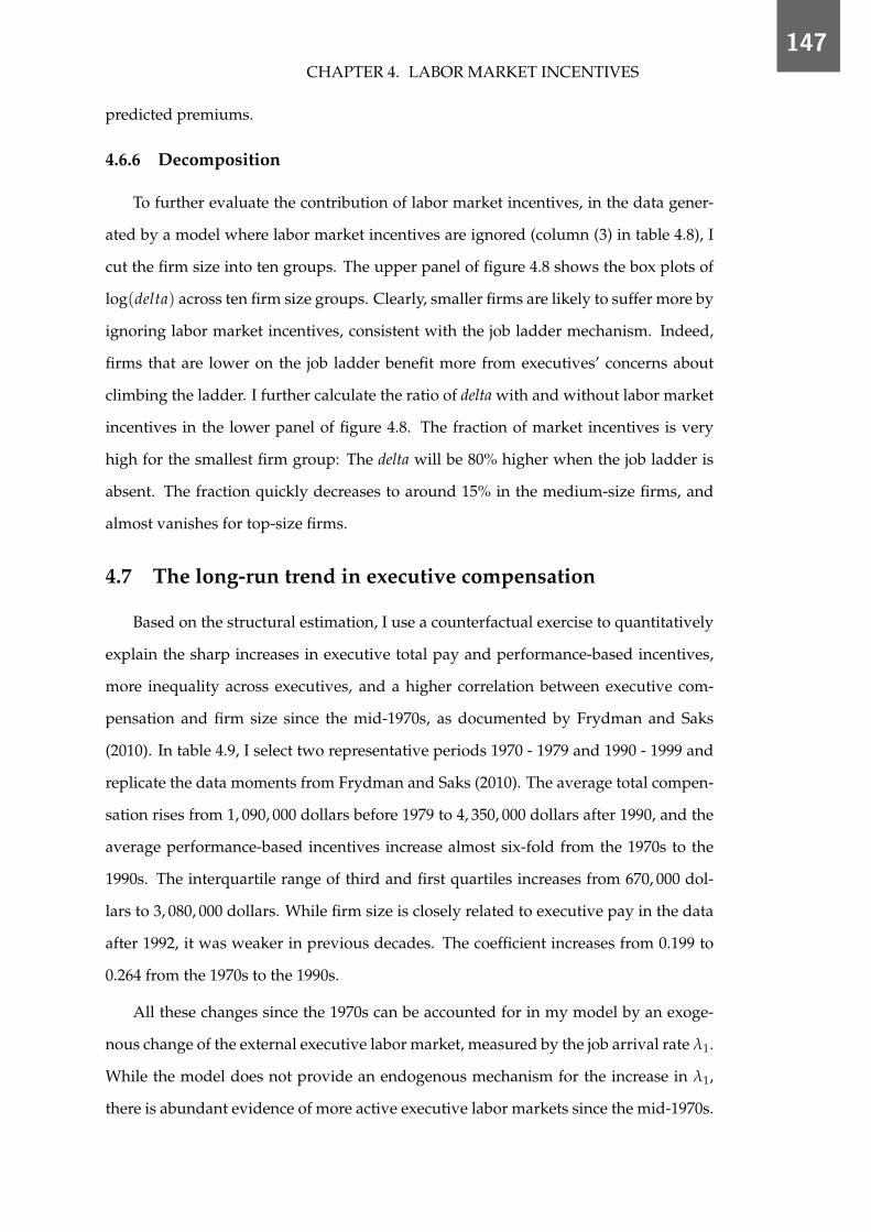
CHAPTER 4. LABOR MARKET INCENTIVES
147
predicted premiums.
4.6.6 Decomposition
To further evaluate the contribution of labor market incentives, in the data gener-
ated by a model where labor market incentives are ignored (column (3) in table 4.8), I
cut the firm size into ten groups. The upper panel of figure 4.8 shows the box plots of
log(delta) across ten firm size groups. Clearly, smaller firms are likely to suffer more by
ignoring labor market incentives, consistent with the job ladder mechanism. Indeed,
firms that are lower on the job ladder benefit more from executives’ concerns about
climbing the ladder. I further calculate the ratio of delta with and without labor market
incentives in the lower panel of figure 4.8. The fraction of market incentives is very
high for the smallest firm group: The delta will be 80% higher when the job ladder is
absent. The fraction quickly decreases to around 15% in the medium-size firms, and
almost vanishes for top-size firms.
4.7 The long-run trend in executive compensation
Based on the structural estimation, I use a counterfactual exercise to quantitatively
explain the sharp increases in executive total pay and performance-based incentives,
more inequality across executives, and a higher correlation between executive com-
pensation and firm size since the mid-1970s, as documented by Frydman and Saks
(2010). In table 4.9, I select two representative periods 1970 - 1979 and 1990 - 1999 and
replicate the data moments from Frydman and Saks (2010). The average total compen-
sation rises from 1, 090, 000 dollars before 1979 to 4, 350, 000 dollars after 1990, and the
average performance-based incentives increase almost six-fold from the 1970s to the
1990s. The interquartile range of third and first quartiles increases from 670, 000 dol-
lars to 3, 080, 000 dollars. While firm size is closely related to executive pay in the data
after 1992, it was weaker in previous decades. The coefficient increases from 0.199 to
0.264 from the 1970s to the 1990s.
All these changes since the 1970s can be accounted for in my model by an exoge-
nous change of the external executive labor market, measured by the job arrival rate λ1.
While the model does not provide an endogenous mechanism for the increase in λ1,
there is abundant evidence of more active executive labor markets since the mid-1970s.

1484.7. THE LONG-RUN TREND IN EXECUTIVE COMPENSATION
0 1 2 3 4 5 6 7 8 9firm size (in 10 groups)
0
2
4
6
8
10
12
log
of d
elta
The benchmark modelThe model ignoring market incentives
0 1 2 3 4 5 6 7 8 9firm size (in 10 groups)
0.0
0.2
0.4
0.6
0.8
1.0
chan
ge o
f del
ta (i
n %
)
Figure 4.8: Fraction of market incentives is higher in smaller firms

CHAPTER 4. LABOR MARKET INCENTIVES
149
Murphy and Zabojnik (2007) document that an increasing number of CEO openings
have been filled through external hires. Huson et al. (2001) document that the fraction
of outsider CEOs increased from 15.3% in the 1970s to 30.0% at the beginning of the
1990s. One explanation for the trend is that executive jobs have increasingly placed
greater emphasis on general rather than firm-specific skills (Frydman 2005). This is
also the view taken by this paper. The executive productivity in the model is “general”
and “transferable” between firms.
For the exercise, I calibrate λ1 to be 5% for 1970 - 1979 and 40% for 1990 - 1999.
These values are chosen to match the data moments under the constraint that all other
parameters are equal to the estimated values in the structural estimation. Since most
firms in the sample of Frydman and Saks (2010) are within the top 500, I keep the largest
500 firms in the simulated data as well. The moments calculated by model-simulated
datasets are reported in the last two columns of table 4.9.
Table 4.9: Long-run trend in executive compensation
Moments Data Model
(dollar value in year 2000) 1970 - 1979 1990 - 1999 λ1 = 0.05 λ1 = 0.4
Mean tdc1 (thousand) 1090 4350 985 4296Mean size (million) - - 2426 5710Mean delta (thousand) 21.743 120.342 24.972 125.310βtdc1−size 0.199 0.264 0.175 0.240
Percentiles of tdc1 (thousand)
25th percentile 640 1350 109 121750th percentile 930 2360 478 295775th percentile 1310 4430 1596 5860
The results are consistent with the model intuition and are quantitatively matched
with the counterparts in data. As λ1 increases, executives are more likely to use poach-
ing offers to renegotiate contracts, which leads to higher total compensation tdc1 (from
985, 000 dollars to 4, 296, 000 dollars) and higher incentives delta (from 24, 972 dollars to
125, 310 dollars for a 1%increase in fir’s rate of return). Moreover, as firms bid for exec-
utives, the correlation between pay and firm size becomes larger (from 0.175 to 0.240).
Finally, since the executive labor market in the model is search-frictional, inequality is
amplified with more poaching offers: Lucky executives receive many poaching offers,

1504.8. THE SPILLOVER EFFECT AND POLICY IMPLICATIONS
while unlucky ones get few job-hopping opportunities.26
My model also entails predictions for moments that are not disclosed in Frydman
and Saks (2010). A more active labor market also induces a larger average firm size.
The mean of firm size doubles as λ1 increases (from 2,425 million to 5,710 million).
The predictions for firm-size pay-growth and incentive premiums (not shown in table
4.9) follow a similar pattern as in the last two columns of table 4.8. These predictions
require further examination in the data.
4.8 The spillover effect and policy implications
In this section, I discuss the spillover effect of firms’ willingness to bid for exec-
utives using comparative statics. The parameter α0 in the production function of the
model represents the firm’s (or the board’s) willingness to pay for executives. The
“spillover” refers to the effect where higher bids from some firms not only raises ex-
ecutive pay in those firms but also increases pay in all firms that are higher on the job
ladder. This is because executives who are higher on the job ladder can make use of
these bids to negotiate with their present firms. Consequently, the renegotiation leads
to higher pay and higher performance-based incentives.
From the perspective of a regulator, executive pay is an essential part of corporate
governance and is often determined by a company’s board of directors. When com-
pensation is inefficient, it is usually a symptom of an underlying governance problem
brought on by conflicted boards and dispersed shareholders. For this reason, I assume
that α0 is negatively correlated with the quality of corporate governance. For example,
an entrenched executive tends to have higher bargaining power and face a higher α0,
while a more independent board may impose a lower α0 on executives. A caveat of this
assumption must be emphasized: It is by no means that α0 should always be negatively
correlated with the quality of governance. This assumption should be valid only in the
range where α0 is too big.
Quantitatively, I use counterfactuals of higher α0 values in firms of different size
to evaluate how sizable such spillover effect can be. I consider two counterfactual
26While the simulated moments are mostly very close to the data, there are some exceptions. In partic-ular, the model generates much lower tdc1 in the first two percentiles when λ1 = 0.05. This may indicatethat the poaching offer distributions of the 1970s and 1990s are different. Thus, separate estimations arerequired for different periods.

CHAPTER 4. LABOR MARKET INCENTIVES
151
1 2 3 4 5 6 7 8 9 10firm size (10 groups)
0
2
4
6
8
10
12
log
of d
elta
The model with worse governance in small firmsThe Benchmark ModelThe model with worse governance in large firms
1 2 3 4 5 6 7 8 9 10firm size (10 groups)
4
5
6
7
8
9
10
11
log
of to
tal c
ompe
nsat
ion
Figure 4.9: Compare higher bids from small/medium firms and from large firms

1524.9. CONCLUSIONS
scenarios. In one scenario, α0 doubles for firms that are smaller than the size median,
the “small/medium firms”. I denote this higher bid of small/medium firms as “worse
governance in small firms”. And it supposes to create a spillover effect on the pay of
large firms. To compare this spillover effect, I use the second counterfactual that α0
doubles for firms that are larger than the median. And this case is denoted as “worse
governance in large firms”. Figure 4.9 plots the distribution of delta (in the upper
panel) and total compensation (in the lower panel) across ten equally divided firm size
groups. There are three box plots for each size group, i.e., worse governance in small
firms, the benchmark model and worse governance in large firms, and the medians are
marked as a horizontal line in the middle of each box.
Not surprisingly, the boosts in bids increase total compensation and incentives in
each separate type of firms. A higher bidding willingness in small/medium firms (in
green) raises pay and incentives in firms of the first five groups, while a higher α0
in large firms (in blue) increases pay and incentives in the largest five groups. Impor-
tantly, the rise in α0 in small/medium firms spillovers to large firms as well. In terms of
median, this spillover effect is as large as the effect of higher bids from large firms them-
selves. As shown in figure 4.9, there are 40% to 50% increases in pay and incentives of
the largest two groups of firms, in both cases of higher bids from small/medium firms
and higher bids from large firms.
The policy implications of this exercise are as follow. To regulate the compensation
of highly paid executives, rather than only focusing on large firms, it is important to
lower the bids in small/ medium firms. Thus, large firms will face less competitive
pressure. As for particular regulation policies, reforms that have been proposed or im-
plemented including more independent compensation committee, greater mandatory
pay (or pay ratio) disclosure, say-on-pay legislation should work in small and medium
firms as well.
4.9 Conclusions
This paper has studied the impact of labor market competition on managerial in-
centive contracts. I developed a dynamic contracting model where executives use
poaching offers to renegotiate with the current firm and showed that poaching offers
have both a level and an incentive effect on compensation. The model explains the

CHAPTER 4. LABOR MARKET INCENTIVES
153
firm-size pay-growth premium and incentive premium. Empirical evidence from a
new dataset on job turnovers supports the job ladder mechanism.
I structurally estimated the model without explicitly targeting firm-size pay-growth
and incentive premiums, yet the predicted premiums of the model match up very
closely with the estimates in the data. A counterfactual analysis based on the structural
estimation showed that with an exogenous increase of poaching offer arrival rate, my
model can account for the sharp increase in total pay, performance-based incentives,
and the correlation between firm size and pay levels since the mid-1970s.
Quantitative analysis showed that there is a spillover effect from the deterioration
of corporate governance in small and medium firms to the compensation growth of
the overall executive labor market. The policy implication is that to regulate the com-
pensation of highly paid executives especially in large firms, it is important to improve
the corporate governance of small and medium firms and reduce their bids. This will
lower the competitive pressure faced by board members of large firms.

1544.A. MODEL APPENDICES
4.A Model appendicesProof for proposition 4.2
I start with a lemma showing that I(
W(z′, s))
is a weighted sum of ∆W(z′,s)∆z′ over
the domain of z′. And then show ∆W(z′,s)∆z′ decreases in s.
Step 1: Prove that I(
W(z′, s))
is a weighted sum of ∆W(z′,s)∆z′
Lemma 4.1. Consider a productivity set Z = {z(1), z(2), ..., z(nz)}. Suppose there is a distri-bution of productivity when the executive takes the effort Γ, a distribution when the executiveshirks Γs, a likelihood ratio g = Γ/Γs and a value function W. All functions are defined on Z,then the incentive that the executive receives from W is
I(
W(z))=
nz−1
∑i=1
ωi∆W(z(i))
∆z(i),
where ∆z(i) = z(i+1) − z(i) and ωi ≥ 0.
Proof. Without lose of generality, I assume g(z) ≥ 1 for z ∈ {z(1), z(2), ..., z(m)} andg(z) < 1 for z ∈ {z(m+1), ..., z(nz)} where m < nz, and define γ(z) ≡ |1− g(z)| × Γ(z).I further denote W(z(i)) by Wi and γ(z(i)) by γi. Moreover, ∑z∈Z(1− g(z))Γ(z) = 0implies that
γ1 + ... + γm − γm+1 − ...− γnz−1 − γnz = 0. (4.11)
It follows that
I(
W)= ∑
z∈Z
(W(z)(1− g(z))Γ(z)
)=− γ1W1 − γ2W2 − ...− γWm + γm+1Wm+1 + γnzWnz
=γ1(W2 −W1) + (γ1 + γ2)(W3 −W2) + ...+ (γ1 + ... + γm)(Wm+1 −Wm) + (γ1 + ... + γm − γm+1)(Wm+2 −Wm+1) + ...+ (γ1 + ... + γm − γm+1 − ...− γnz−1)(Wnz −Wnz−1)
+ (γ1 + ... + γm − γm+1 − ...− γnz−1 − γnz)Wnz
=γ1∆z1W2 −W1
∆z1+ (γ1 + γ2)∆z2
(W3 −W2)
∆z2+ ...
+ (γ1 + ... + γm)∆zm(Wm+1 −Wm)
∆zm
+ (γ1 + ... + γm − γm+1)∆zm+1Wm+2 −Wm+1
∆zm+1+ ...
+ (γ1 + ... + γm − γm+1 − ...− γnz−1 − γnz−1)∆znz−1Wnz −Wnz−1
∆znz−1
=ω1W2 −W1
∆z1+ ω2
(W3 −W2)
∆z2+ ...
+ ωm(Wm+1 −Wm)
∆zm+ ωm+1
Wm+2 −Wm+1
∆zm+1+ ... + ωnz−1
Wnz −Wnz−1
∆znz−1
=nz−1
∑i=1
ωi∆W(z(i))
∆z(i).
The first equality follows from the definition of the incentive operator I , the reststeps are simple algebraic transformations, where I have applied condition (4.11). Byconstruction, ωi is positive.

CHAPTER 4. LABOR MARKET INCENTIVES
155
Step 2: Express ∆W(z,s)∆z in terms of s.
Given lemma 1, it is sufficient to show that ∆W(z,s)∆z decreases in s for all z ∈ Z. Notice
that
∆W(z, s)∆z
= − ∆Π(z, s, W)/∆z∆Π(z, s, W)/∆W
= u′(w(s))∆Π(z, s, W)
∆z, (4.12)
where w(z, s) is the compensation corresponding to W(z, s) and satisfies (4.1).To derive w, suppose the effort cost is
c = c(s) ≡ β ∑z′∈Z
W(z′, s)(1− g(z′|z))Γ(z′|z),
such that the optimal contract indicates that the promised value equals the biddingfrontier
W(z′, s) = W(z′, s).Under the optimal contract, the continuation value (profit) of the firm is zero.
According to the Bellman equation of the firm,
Π(z, s, W(z, s)) = ∑z′∈Z
(α0sα1 z′ − w + β
∫s
Π(z′, s, W(z′, s)dF(s))
Γ(z′|z)
= ∑z′∈Z
(α0sα1 − w + β
∫s
Π(z′, s, W(z′, s)dF(s))
Γ(z′|z)
= ∑z′∈Z
(α0sα1 − w
)Γ(z′|z) = 0.
Therefore,w(z, s) = α0sα1 ∑
z′∈Z
z′Γ(z′|z)
To derive ∆Π(z,s,W)∆z , I use envelop theorem. It follows that
∆Π(z, s, W)
∆z= ∑
z′∈Z
(α0sα1 z′ + β
∫s≤s
Π(z′, s, W(z′, s)dF(s))∆Γ(z′|z)
∆z
+ λβ ∑z′∈Z
( ∫sW(z′, s)dF(s)
)∆Γ(z′|z)∆z
+ µβ ∑z′∈Z
( ∫sW(z′, s)dF(s)
)∆((1− g(z′|z)Γ(z′|z)
)∆z
=α0sα1 ∑z′∈Z
z′∆Γ(z′|z)
∆z+ β ∑
z′∈Z
∫sW(z′, s)dF(s)
(λ
∆Γ(z′|z)∆z
+ µ∆((1− g(z′|z)Γ(z′|z)
)∆z
).
(4.13)
Divide both sides by α0 ∑z′∈Z z′ ∆Γ(z′|z)∆z , we have
∆Π(z,s,W)∆z
α0 ∑z′∈Z z′ ∆Γ(z′|z)∆z
=sα1 + ψ(s), (4.14)

1564.A. MODEL APPENDICES
where ψ(s) ≡β ∑z′∈Z
∫s W(z′,s)dF(s)
(λ
∆Γ(z′ |z)∆z +µ
∆
((1−g(z′ |z)Γ(z′ |z)
)∆z
)∆z /α ∑z′∈Z z′ ∆Γ(z′|z)
∆z .Since all items of ψ(s) are positive, ψ(s) > 0. Because ψ(s) only depends on s via
W which is increasing in s, ψ(s) is also increasing in s.Insert (4.13) and (4.14) into (4.12), we have
∆W(z, s)∆z
= u′(w(s))∆Π(z, s, W)
∆z= u′
(α0sα1 ∑
z′∈Z
z′Γ(z′|z))(
sα1 + ψ(s))
α0 ∑z′∈Z
z′∆Γ(z′|z)
∆z.
(4.15)
Step 3: Show that ∆W(z,s)∆z decreases in s under the stated condition in the proposition.
To have
lim∆s→0
∆W(z, s + ∆s)∆z
− ∆W(z, s)∆z
> 0,
using (4.15), we have
u′((s + ∆s)α1 α0 ∑z′∈Z z′Γ(z′|z)
)u′(
sα1 α0 ∑z′∈Z z′Γ(z′|z)) <
sα1 + ψ(s)(s + ∆s)α1 + ψ(s + ∆s)
.
Applying u′(w) = w−σ, we have( ss + ∆s
)−α1σ<
sα1 + ψ(s)(s + ∆s)α1 + ψ(s + ∆s)
,
or
σ >log sα1+ψ(s)
(s+∆s)α1+ψ(s+∆s)s
s+∆s.
Taking ∆s→ 0 using L’Hopital’s rule, we have
σ > 1 +s1−α1
α1ψ′(s).

CHAPTER 4. LABOR MARKET INCENTIVES
157
4.B Empirical appendicesThis appendix contains some extra regression results on firm-size incentive pre-
mium. Figure 4.10 is a heat map of performance-based incentives log(delta) on totalcompensation and firm size. It shows that among executives with similar total com-pensation, those in larger firms get higher performance-based incentives. Table 4.10contains the full results of the size incentive premium for each age.
dollar−percent incentives (data)
total compensation
firm
siz
e
0
10
20
30
40
50
60
70
0 10 20 30 40 50 60 70
0.7
2
3.2
4.5
5.8
7.1
8.3
9.6
Figure 4.10: log(delta) over firm size and total compensation
Note: delta is the wealth-performance sensitivity defined as the dollar change in firm-related wealthfor a percentage change in firm value. The total compensation is the sum of salary and bonus, thevalue of restricted stocks and options granted, and the value of retirement and long-term compen-sation schemes. The firm size is the market capitalization by the end of the fiscal year, calculated bycsho× prcc f where csho is the common shares outstanding and prcc f is the close price by fiscalyear. I divide the whole sample into 80× 80 cells according to the total compensation and firm sizeand compute the mean of log(delta) within each cell.

1584.B. EMPIRICAL APPENDICES
Table 4.10: Size incentive premium decreases with executive age
log(delta)(1) (2) (3) (4) (5)
age35 × log(firm size) 0.849∗∗∗ 0.652∗∗∗ 0.580∗∗∗ 0.541∗∗∗ 0.539∗∗∗(0.0534) (0.0649) (0.0620) (0.0614) (0.0611)
age36 × log(firm size) 0.753∗∗∗ 0.530∗∗∗ 0.516∗∗∗ 0.484∗∗∗ 0.481∗∗∗(0.0487) (0.0658) (0.0519) (0.0538) (0.0529)
age37 × log(firm size) 0.746∗∗∗ 0.543∗∗∗ 0.540∗∗∗ 0.508∗∗∗ 0.506∗∗∗(0.0366) (0.0440) (0.0359) (0.0365) (0.0365)
age38 × log(firm size) 0.689∗∗∗ 0.471∗∗∗ 0.471∗∗∗ 0.438∗∗∗ 0.436∗∗∗(0.0328) (0.0390) (0.0339) (0.0341) (0.0332)
age39 × log(firm size) 0.667∗∗∗ 0.444∗∗∗ 0.443∗∗∗ 0.410∗∗∗ 0.410∗∗∗(0.0276) (0.0365) (0.0297) (0.0297) (0.0296)
age40 × log(firm size) 0.664∗∗∗ 0.475∗∗∗ 0.493∗∗∗ 0.462∗∗∗ 0.461∗∗∗(0.0296) (0.0358) (0.0319) (0.0341) (0.0338)
age41 × log(firm size) 0.653∗∗∗ 0.449∗∗∗ 0.489∗∗∗ 0.459∗∗∗ 0.457∗∗∗(0.0264) (0.0350) (0.0320) (0.0325) (0.0324)
age42 × log(firm size) 0.640∗∗∗ 0.437∗∗∗ 0.478∗∗∗ 0.453∗∗∗ 0.450∗∗∗(0.0285) (0.0342) (0.0330) (0.0338) (0.0335)
age43 × log(firm size) 0.630∗∗∗ 0.408∗∗∗ 0.469∗∗∗ 0.445∗∗∗ 0.444∗∗∗(0.0248) (0.0333) (0.0303) (0.0311) (0.0309)
age44 × log(firm size) 0.622∗∗∗ 0.405∗∗∗ 0.473∗∗∗ 0.449∗∗∗ 0.447∗∗∗(0.0230) (0.0345) (0.0313) (0.0314) (0.0314)
age45 × log(firm size) 0.608∗∗∗ 0.397∗∗∗ 0.468∗∗∗ 0.447∗∗∗ 0.446∗∗∗(0.0220) (0.0287) (0.0280) (0.0280) (0.0278)
age46 × log(firm size) 0.592∗∗∗ 0.377∗∗∗ 0.443∗∗∗ 0.424∗∗∗ 0.422∗∗∗(0.0210) (0.0293) (0.0283) (0.0286) (0.0284)
age47 × log(firm size) 0.594∗∗∗ 0.365∗∗∗ 0.445∗∗∗ 0.428∗∗∗ 0.426∗∗∗(0.0207) (0.0297) (0.0289) (0.0296) (0.0295)
age48 × log(firm size) 0.598∗∗∗ 0.367∗∗∗ 0.454∗∗∗ 0.435∗∗∗ 0.434∗∗∗(0.0163) (0.0259) (0.0252) (0.0256) (0.0257)
age49 × log(firm size) 0.594∗∗∗ 0.369∗∗∗ 0.437∗∗∗ 0.419∗∗∗ 0.417∗∗∗(0.0180) (0.0264) (0.0284) (0.0276) (0.0277)
age50 × log(firm size) 0.589∗∗∗ 0.388∗∗∗ 0.457∗∗∗ 0.439∗∗∗ 0.438∗∗∗(0.0210) (0.0287) (0.0301) (0.0316) (0.0317)
age51 × log(firm size) 0.563∗∗∗ 0.352∗∗∗ 0.426∗∗∗ 0.410∗∗∗ 0.409∗∗∗(0.0173) (0.0254) (0.0270) (0.0273) (0.0275)
age52 × log(firm size) 0.560∗∗∗ 0.342∗∗∗ 0.414∗∗∗ 0.399∗∗∗ 0.398∗∗∗(0.0191) (0.0268) (0.0280) (0.0282) (0.0281)
age53 × log(firm size) 0.577∗∗∗ 0.350∗∗∗ 0.425∗∗∗ 0.409∗∗∗ 0.408∗∗∗(0.0192) (0.0274) (0.0278) (0.0286) (0.0287)
age54 × log(firm size) 0.570∗∗∗ 0.335∗∗∗ 0.423∗∗∗ 0.409∗∗∗ 0.409∗∗∗(0.0209) (0.0288) (0.0286) (0.0290) (0.0293)
age55 × log(firm size) 0.569∗∗∗ 0.351∗∗∗ 0.435∗∗∗ 0.423∗∗∗ 0.423∗∗∗(0.0184) (0.0279) (0.0271) (0.0273) (0.0273)

CHAPTER 4. LABOR MARKET INCENTIVES
159
Table 4.10: Size incentive premium decreases with executive age (continue)
(1) (2) (3) (4) (5)
age56 × log(firm size) 0.592∗∗∗ 0.362∗∗∗ 0.454∗∗∗ 0.442∗∗∗ 0.441∗∗∗(0.0157) (0.0260) (0.0271) (0.0272) (0.0270)
age57 × log(firm size) 0.593∗∗∗ 0.356∗∗∗ 0.440∗∗∗ 0.429∗∗∗ 0.428∗∗∗(0.0141) (0.0233) (0.0237) (0.0232) (0.0230)
age58 × log(firm size) 0.592∗∗∗ 0.356∗∗∗ 0.442∗∗∗ 0.430∗∗∗ 0.429∗∗∗(0.0175) (0.0266) (0.0261) (0.0260) (0.0261)
age59 × log(firm size) 0.593∗∗∗ 0.351∗∗∗ 0.435∗∗∗ 0.423∗∗∗ 0.422∗∗∗(0.0172) (0.0256) (0.0258) (0.0253) (0.0254)
age60 × log(firm size) 0.579∗∗∗ 0.341∗∗∗ 0.424∗∗∗ 0.412∗∗∗ 0.412∗∗∗(0.0175) (0.0271) (0.0259) (0.0258) (0.0259)
age61 × log(firm size) 0.600∗∗∗ 0.355∗∗∗ 0.438∗∗∗ 0.428∗∗∗ 0.427∗∗∗(0.0216) (0.0307) (0.0302) (0.0311) (0.0309)
age62 × log(firm size) 0.587∗∗∗ 0.333∗∗∗ 0.420∗∗∗ 0.409∗∗∗ 0.408∗∗∗(0.0192) (0.0282) (0.0268) (0.0272) (0.0272)
age63 × log(firm size) 0.605∗∗∗ 0.358∗∗∗ 0.448∗∗∗ 0.436∗∗∗ 0.435∗∗∗(0.0196) (0.0252) (0.0256) (0.0253) (0.0255)
age64 × log(firm size) 0.593∗∗∗ 0.356∗∗∗ 0.440∗∗∗ 0.429∗∗∗ 0.429∗∗∗(0.0242) (0.0285) (0.0296) (0.0292) (0.0289)
age65 × log(firm size) 0.596∗∗∗ 0.353∗∗∗ 0.435∗∗∗ 0.423∗∗∗ 0.423∗∗∗(0.0246) (0.0318) (0.0339) (0.0334) (0.0332)
logtdc1 0.611∗∗∗ 0.345∗∗∗(0.0352) (0.0339)
tdc1 Dummies (50) Yestdc1 Dummies (100) Yesprofit 0.619∗∗∗ 0.598∗∗∗ 0.602∗∗∗
(0.117) (0.116) (0.116)annual return 0.102∗ 0.0999 0.0998
(0.0488) (0.0485) (0.0485)mbr 0.116∗∗∗ 0.120∗∗∗ 0.120∗∗∗
(0.0209) (0.0213) (0.0213)director 0.754∗∗∗ 0.739∗∗∗ 0.737∗∗∗
(0.0326) (0.0307) (0.0306)interlock 0.517∗∗∗ 0.529∗∗∗ 0.527∗∗∗
(0.0953) (0.0948) (0.0947)CEO 0.593∗∗∗ 0.576∗∗∗ 0.574∗∗∗
(0.0387) (0.0395) (0.0397)CFO 0.0837∗∗∗ 0.0711∗∗∗ 0.0711∗∗∗
(0.0130) (0.0131) (0.0130)N 146750 128008 109732 109732 109732adj. R2 0.432 0.506 0.586 0.590 0.590

1604.B. EMPIRICAL APPENDICES
Note: This table reports the evidence that firm size incentive premium decreases in ex-ecutive age. The dependent variable is the log of delta where delta is the dollar changein firm-related wealth for a percentage change in firm value. The key independentvariable is the log of firm size where firm size is measured by the market capitalizationdefined by the common shares outstanding times the fiscal year close price. I allow dif-ferent coefficients of firm size across ages from 35 to 65. Control variables include totalcompensation (tdc1), age dummies, executive tenure dummies, year times industrydummies, profit, the operating profitability, mbr, the market-book ratio, annual return,the annualized stock return, director, whether the executive served as a director duringthe fiscal year, CEO and CFO, whether the executive served as a CEO (and CFO) duringthe fiscal year, interlock, whether the executive is involved in the interlock relationship.Standard error (clustered at the firm × fiscal year level) are shown in parentheses, andI denote symbols of significance by ∗ p < 0.05, ∗∗ p < 0.01 and ∗∗∗ p < 0.001.
CHAPTER 4. LABOR MARKET INCENTIVES
161
4.C EstimationRecursive multiplier method
To further characterize the optimal solution, I resort to the tools developed byMarcet and Marimon (2017).27In dynamic contracting problems with forward-lookingconstraints such as the IC constraint here, the solution does not satisfy the Bellmanequation. MM suggest studying a recursive Lagrangian. Under standard general con-ditions, there is a recursive saddle-point functional equation (analogous to a Bellmanequation) that characterizes a recursive solution to the planner’s problem. The recur-sive formulation is obtained after adding a co-state variable λt summarizing previouscommitments reflected in past Lagrange multipliers. The time-consistent continuationsolution is obtained by using the endogenous λt as the vector of weights in the objectivefunction. I summarize this method in the following proposition.
Proposition 4.3 (Marcet and Marimon). Define Pareto Frontier by
P(z, s, λ) = supW
Π(z, s, W) + λW,
where Π and W are defined as in (BE-F) and (PKC), and λ > 0 is a Pareto weight assigned tothe executive. Then there exist positive multipliers of {µ, µ0(z′), µ1(z′)} that solve the follow-ing problem
P(z, s, λ) = infµ,µ0(z′,s),µ1(z′,s)
supw
h(z, s, λ, w) + β ∑z′
P(z′, s, λ′)Γ(z′|z),
where multiplier µ corresponds to the incentive compatibility constraint, multipliers µ0(z′, s), µ1(z′, s)correspond to participation constraints,
h(z, s, λ, w) = y(s)z′ − w + λu(w)− (λ + µ)c,
Pareto weight evolves according to
λ′ = λ + µ(1− g(z, z′)) + µ0(z′, s) + µ1(z′, s),
andβ = β(1− λ1 ∑
M1∪M2
F(s′)).
The optimal contract {w, W(z′, s)} follows that
u′(w) =1λ
, (4.16)
W(z′, s) = W(z′, s, λ′). (4.17)
Proposition 4.3 can be illustrated intuitively using the Pareto weight of the execu-tive λ and the multiplier µ of the incentive constraint. Suppose the match starts witha λ(0), and assume the participation constraints are not binding so that µ0 = µ1 = 0.λ(0) has to satisfy W(zO, s, λ(0)) = W0. To deal with the moral hazard, the optimal con-tract indicates a µ(0) > 0. Then depending on the realization of z′, the weight of theexecutive will be updated to
λ(i) = λ(i−1) + µi−1(1− g(z, z′)) for i in 1, 2... (4.18)
The evolve of λ continues as such till the match breaks.27This approach has been used in many applications. A few examples are: growth and business cycles
with possible default (Marcet and Marimon (1992), Kehoe and Perri (2002), Cooley, et al. (2004)); socialinsurance (Attanasio and Rios-Rull (2000)); optimal fiscal and monetary policy design with incompletemarkets (Aiyagari, Marcet, Sargent and Seppala (2002), Svensson and Williams (2008)); and political-economy models (Acemoglu, Golosov and Tsyvinskii (2011)).

1624.C. ESTIMATION
When there is an outside offer such that the executive moves from his or her currentfirm to the outside firm, the new match starts with a weight denoted by λ(n) such that
W(z, s, λ(n)) = W(z, s),
where I have denoted the current productivity by z, current firm by s, and the outsidefirm by s. It means the new match will assign a new weight to the executive so that he orshe gets the continuation value W(z, s). Then the new Pareto weight will evolve againas illustrated in (4.18). In a nutshell, proposition 4.3 allows me to solve the optimalcontract in the space of Pareto weight λ instead of in the space of the promised utility.At any moment, I can transit from the metrics of λ back to the metrics of utilities using(4.16) and (4.17).
The advantage of this method is that I do not need to find the promised utilitiesW(z′, s) in each state of the world for the next period. Instead, λ and µ are enoughto trace all W(z′, s). Moreover, λ corresponds to the total compensation level (wagelevel), while µ corresponds to how much contract incentive is provided in the optimalcontract. The two multipliers are enough to understand both theoretically and numer-ically why keeping the same wage level (the same λ), incentive pays increase with firmsize (µ increases with firm size).

Summary
This thesis consists of three studies investigating topics in the fields of intermediaries
and executive compensation through the lens of search frictions. The three studies all
point to the power of the search frictions in explaining real-world phenomena. This
summary provides an overview of the research questions addressed, the methodolo-
gies used to answer those questions, and the conclusions from this research.
Chapter 2 develops a directed search framework to understand two widely used mar-
ket structures of intermediaries: the middleman mode and the marketmaker (or plat-
form) mode. In the middleman mode, the intermediary is specialized in buying and
selling for its own account and typically operates with inventory holdings (e.g., deal-
ers in financial and steel markets). In the marketmaker mode, the intermediary offers
a marketplace for fees, where the participating buyers and sellers can search and trade
with each other (e.g., eBay, brokers in real estate and financial markets). Due to the
search frictions, the intermediary has a trade-off between a larger transaction volume
by operating as a middleman and a higher price/fee by acting as market-maker. This
trade-off determines the optimal intermediation mode, and eventually a marketmaking
middleman such as Amazon, who adopts a mixture of these two intermediation modes,
can be optimal in the equilibrium. Our main insight holds in various market envi-
ronments, including an endowment economy and a market with nonlinear matching
functions. The theoretical predictions are examined using scraped data from Amazon
and eBay.
Chapter 3 contributes to a better understanding of the competition among e-commerce
giants. We extended the framework of Chapter 2 to a Bertrand competition game
between an incumbent intermediary who can mix a middleman and a marketmaker
mode, and an entrant intermediary who is restricted to be a marketmaker. Meeting
163

1644.C. ESTIMATION
technologies in both intermediaries are subjected to search frictions. We find that the
entrant faces the choice of being a second-source (for intermediation service) with high
price/fees and a sole active source by undercutting the incumbent. Despite this strate-
gic complication, we show that the intuition of chapter 2 holds in a duopoly. In partic-
ular, for a reasonable set of parameters, there exists an equilibrium of pure strategies
where a marketmaking middleman incumbent emerges. Furthermore, in the mixed
strategy equilibrium, the incumbent activates its market-maker mode with positive
probability.
Chapter 4 assesses the impact of job search ladders on executives’ incentive contracts.
In the theoretical framework, an executive is poached by outside firms while a dynamic
incentive contract is designed to deal with both the moral hazard problem inside the
firm and competition from the external labor market. I show that competition for ex-
ecutives increases total compensation, and generates a new source of incentives, called
labor market incentives, which substitutes for performance-based incentives embedded
in bonus, stocks, options, etc. The model is estimated using a newly assembled dataset
on job turnovers for executives in U.S. publicly listed firms. Simulations based on the
structural estimates show that the model is capable of explaining and replicating the
puzzling facts that executives of larger firms experience higher compensation growth
and receive higher performance-based incentives.

Samenvatting (Summary in Dutch)
Dit proefschrift bestaat uit drie studies naar onderwerpen op de gebieden van bemid-
deling en bestuurdersbeloningen, allen beschouwd door een zoekfrictiebril. De studies
benadrukken de kracht van zoekfricties in het verklaren van verschijnselen in de echte
wereld. Deze samenvatting biedt een overzicht van de geadresseerde onderzoeksvra-
gen, de methodologien gebruikt om deze onderzoeksvragen te beantwoorden, en de
conclusies van dit onderzoek.
Hoofdstuk 2 ontwikkelt een model om twee veelgebruikte vormen van bemiddeling te
leren begrijpen: de tussenpersoonwijze en de marktmaker- (of platform)wijze. Bij de
tussenpersoonwijze is de bemiddelaar gespecialiseerd in het zelf kopen en verkopen
en maakt deze veelal gebruik van voorraden (bijv. handelaren in financile en staal-
markten). Bij de marktmakerwijze biedt de bemiddelaar tegen betaling een plaats op
de markt aan, waarbij de deelnemende kopers en verkopers kunnen zoeken en met
elkaar kunnen handelen (bijv. eBay, makelaars en handelaren op financile markten).
Door zoekfricties heeft de bemiddelaar te maken met een uitruil tussen een groter
transactievolume bij het als tussenpersoon optreden en een hogere prijs/honorarium
per item bij het als marktmaker optreden. Deze uitruil bepaalt de optimale bemiddel-
ingswijze, en uiteindelijk kan een mengsel van de tussenpersoon- en marktmakerwijze,
zoals Amazon die toepast, optimaal zijn in het evenwicht. Dit geldt voor verschillende
marktomgevingen, inclusief een economie zonder producenten en een markt met niet-
lineaire matching functies. De theoretische voorspellingen worden ondersteund door
empirische testresultaten gebaseerd op data van Amazon en eBay.
Hoofdstuk 3 draagt bij aan een beter begrip van de concurrentie tussen e-commerce
reuzen. We breiden het model van hoofdstuk 2 uit naar een Bertrand concurrentiespel
tussen een gevestigde bemiddelaar welke de tussenpersoon- en markmakerswijze kan
165

1664.C. ESTIMATION
mengen, en een toetredende bemiddelaar welke wordt beperkt tot het zijn van een
marktmaker. Ontmoetingstechnologien voor beide bemiddelaars zijn blootgesteld aan
zoekfricties. We vinden dat de toetreder de keuze heeft tussen het zijn van een se-
cundaire aanbieder (voor bemiddelingsdiensten) met een hoge prijs/honorarium per
item en het zijn van de primaire aanbieder door de gevestigde partij te onderbieden.
Ondanks deze strategische complicatie laten we zien dat de intuiti uit hoofdstuk 2
overeind blijft in een duopolie. In het bijzonder bestaat er, voor een redelijke set van pa-
rameters, een evenwicht in pure strategien waarbij een gevestigde bemiddelaar mark-
tmaker is. Verder is de kans dat de gevestigde bemiddelaar zijn marktmakerwijze ac-
tiveert positief in het evenwicht in gemengde strategien.
Hoofdstuk 4 schat de invloed van baanladders op beloningscontracten van bestuur-
ders. In het theoretische model krijgt een bestuurder aanbiedingen van andere bedri-
jven terwijl een dynamisch beloningscontract de strijd met het moral hazard probleem
binnen het bedrijf en concurrentie van de externe arbeidsmarkt aangaat. Ik laat zien
dat concurrentie om bestuurders leidt tot een stijging van de totale beloning, en dat
het een nieuwe bron van prikkels genereert, genoemd arbeidsmarktprikkels, welke re-
sultaatgerichte prikkels in bonussen, aandelen, opties, etcetera, vervangen. Het model
is geschat met behulp van een nieuw geconstrueerde dataset voor baanwisselingen
van bestuurders van Amerikaanse beursgenoteerde bedrijven. Simulaties gebaseerd
op structurele schattingen laten zien dat het model het verbazingwekkende feit dat
bestuurders van grotere bedrijven grotere beloningsgroei doormaken en een hogere
resultaatgerichte beloning ontvangen, kan verklaren en repliceren.

Bibliography
Abraham, Arpad, Fernando Alvarez-Parra, and Susanne Forstner (2016), “The effectsof moral hazard on wage inequality in a frictional labor market.”
Abreu, Dilip, David Pearce, and Ennio Stacchetti (1990), “Toward a theory of dis-counted repeated games with imperfect monitoring.” Econometrica: Journal of theEconometric Society, 1041–1063.
Acemoglu, Daron and Robert Shimer (1999), “Holdups and efficiency with search fric-tions.” International Economic Review, 40, 827–849.
Agrawal, Ashwini and Alexander Ljungqvist (2014), “Managerial labor market fric-tions and corporate investment.”
Alvarez, Fernando and Urban J Jermann (2000), “Efficiency, equilibrium, and asset pric-ing with risk of default.” Econometrica, 68, 775–797.
Anand, Amber, Carsten Tanggaard, and Daniel G Weaver (2009), “Paying for marketquality.” Journal of Financial and Quantitative Analysis, 44, 1427–1457.
Armstrong, Mark (2006), “Competition in two-sided markets.” The RAND Journal ofEconomics, 37, 668–691.
Armstrong, Mark and Jidong Zhou (2015), “Search deterrence.” The Review of EconomicStudies, 83, 26–57.
Awaya, K. Iwahashi, Y. and M. Watanabe (2018a), “Speculative bubbles in an economywith flippers.” mimeo.
Awaya, Z. Chen, Y. and M. Watanabe (2018b), “Intermediation and reputation.” mimeo.
Baker, George P and Brian J Hall (2004), “Ceo incentives and firm size.” Journal of LaborEconomics, 22, 767–798.
Baye, Michael R and John Morgan (2001), “Information gatekeepers on the internet andthe competitiveness of homogeneous product markets.” American Economic Review,91, 454–474.
Biglaiser, Gary (1993), “Middlemen as experts.” The RAND journal of Economics, 212–223.
Bloch, Francis and Harl Ryder (2000), “Two-sided search, marriages, and matchmak-ers.” International Economic Review, 41, 93–116.
Bohm, Michael J, Daniel Metzger, and Per Stromberg (2015), “’since you’re so rich, youmust be really smart’: Talent and the finance wage premium.”
Burdett, Kenneth, Shouyong Shi, and Randall Wright (2001), “Pricing and matchingwith frictions.” Journal of Political Economy, 109, 1060–1085.
Butters, Gerard R et al. (1977), “Equilibrium distributions of sales and advertisingprices.” Review of Economic Studies, 44, 465–491.
Cahuc, Pierre, Fabien Postel-Vinay, and Jean-Marc Robin (2006), “Wage bargainingwith on-the-job search: Theory and evidence.” Econometrica, 74, 323–364.
167
168BIBLIOGRAPHY
Caillaud, Bernard and Bruno Jullien (2001), “Competing cybermediaries.” EuropeanEconomic Review, 45, 797–808.
Caillaud, Bernard and Bruno Jullien (2003), “Chicken & egg: Competition among inter-mediation service providers.” RAND journal of Economics, 309–328.
Coles, Jeffrey L, Naveen D Daniel, and Lalitha Naveen (2006), “Managerial incentivesand risk-taking.” Journal of financial Economics, 79, 431–468.
Coles, Jeffrey L, Naveen D Daniel, and Lalitha Naveen (2013), “Calculation of com-pensation incentives and firm-related wealth using execucomp: Data, program, andexplanation.”
Condorelli, Daniele, Andrea Galeotti, and Vasiliki Skreta (2018), “Selling through refer-rals.” Journal of Economics & Management Strategy, 27, 669–685.
Conroy, Robert M and Robert L Winkler (1986), “Market structure: The specialist asdealer and broker.” Journal of Banking & Finance, 10, 21–36.
Cornelli, Francesca, Zbigniew Kominek, and Alexander Ljungqvist (2013), “Monitor-ing managers: Does it matter?” The Journal of Finance, 68, 431–481.
Custodio, Claudia, Miguel A Ferreira, and Pedro Matos (2013), “Generalists versus spe-cialists: Lifetime work experience and chief executive officer pay.” Journal of FinancialEconomics, 108, 471–492.
Damiano, Ettore and Hao Li (2008), “Competing matchmaking.” Journal of the EuropeanEconomic Association, 6, 789–818.
Dasgupta, Partha and Eric Maskin (1986), “The existence of equilibrium in discontinu-ous economic games, ii: Applications.” Review of Economic Studies, 53, 27–41.
Dasgupta, Partha, Eric Maskin, et al. (1986), “The existence of equilibrium in discontin-uous economic games, i: Theory.” Review of Economic Studies, 53, 1–26.
De Fraja, Gianni and Jozsef Sakovics (2012), “Exclusive nightclubs and lonely heartscolumns: non-monotone participation in optional intermediation.” Journal of Eco-nomic Behavior & Organization, 84, 618–632.
De los Santos, Babur, Ali Hortacsu, and Matthijs R Wildenbeest (2012), “Testing modelsof consumer search using data on web browsing and purchasing behavior.” AmericanEconomic Review, 102, 2955–80.
Dittmann, Ingolf and Ernst Maug (2007), “Lower salaries and no options? on the opti-mal structure of executive pay.” The Journal of Finance, 62, 303–343.
Dittmann, Ingolf, Ernst Maug, and Oliver Spalt (2010), “Sticks or carrots? optimal ceocompensation when managers are loss averse.” The Journal of Finance, 65, 2015–2050.
Dittmann, Ingolf, Ko-Chia Yu, and Dan Zhang (2017), “How important are risk-takingincentives in executive compensation?” Review of Finance, 21, 1805–1846.
Duffie, Darrell, Nicolae Garleanu, and Lasse Heje Pedersen (2005), “Over-the-countermarkets.” Econometrica, 73, 1815–1847.
Edelman, Benjamin, Julian Wright, et al. (2015), “Price restrictions in multi-sided plat-forms: Practices and responses.” Harvard Business School NOM Unit Working Paper.
Edmans, Alex and Xavier Gabaix (2011), “The effect of risk on the ceo market.” TheReview of Financial Studies, 24, 2822–2863.
Edmans, Alex, Xavier Gabaix, and Dirk Jenter (2017), “Executive compensation: Asurvey of theory and evidence.” Technical report, National Bureau of Economic Re-search.

BIBLIOGRAPHY
169
Edmans, Alex, Xavier Gabaix, and Augustin Landier (2009), “A multiplicative modelof optimal ceo incentives in market equilibrium.” The Review of Financial Studies.
Eisfeldt, Andrea L and Camelia M Kuhnen (2013), “Ceo turnover in a competitive as-signment framework.” Journal of Financial Economics, 109, 351–372.
Fama, Eugene F (1980), “Agency problems and the theory of the firm.” Journal of politicaleconomy, 88, 288–307.
Farhi, Emmanuel and Ivan Werning (2013), “Insurance and taxation over the life cycle.”Review of Economic Studies, 80, 596–635.
Fingleton, John (1997), “Competition among middlemen when buyers and sellers cantrade directly.” The journal of industrial economics, 45, 405–427.
Frydman, Carola (2005), “Rising through the ranks. the evolution of the market forcorporate executives, 1936-2003.” Working Paper.
Frydman, Carola and Raven E Saks (2010), “Executive compensation: A new view froma long-term perspective, 1936–2005.” The Review of Financial Studies, 23, 2099–2138.
Gabaix, Xavier and Augustin Landier (2008), “Why has ceo pay increased so much?”The Quarterly Journal of Economics, 123, 49–100.
Galeotti, Andrea and Jose Luis Moraga-Gonzalez (2009), “Platform intermediation in amarket for differentiated products.” European Economic Review, 53, 417–428.
Gautier, Pieter A, Bo Hu, and Makoto Watanabe (2018), “Marketmaking middlemen.”CEPR Discussion Paper.
Gautier, Pieter A and Coen N Teulings (2015), “Sorting and the output loss due tosearch frictions.” Journal of the European Economic Association, 13, 1136–1166.
Gautier, Pieter A, Coen N Teulings, and Aico Van Vuuren (2010), “On-the-job search,mismatch and efficiency.” The Review of Economic Studies, 77, 245–272.
Gayle, George-Levi, Limor Golan, and Robert A Miller (2015), “Promotion, turnover,and compensation in the executive labor market.” Econometrica, 83, 2293–2369.
Gayle, George-Levi and Robert A Miller (2009), “Has moral hazard become a moreimportant factor in managerial compensation?” American Economic Review, 99, 1740–69.
Gehrig, Thomas (1993), “Intermediation in search markets.” Journal of Economics &Management Strategy, 2, 97–120.
Geromichalos, Athanasios and Kuk Mo Jung (2018), “An over-the-counter approach tothe forex market.” International Economic Review, 59, 859–905.
Giannetti, Mariassunta (2011), “Serial ceo incentives and the structure of managerialcontracts.” Journal of Financial Intermediation, 20, 633–662.
Gibbons, Robert and Kevin J Murphy (1992), “Optimal incentive contracts in the pres-ence of career concerns: Theory and evidence.” Journal of political Economy, 100, 468–505.
Grochulski, Borys and Yuzhe Zhang (2017), “Market-based incentives.” InternationalEconomic Review, 58, 331–382.
Guerrieri, Veronica, Robert Shimer, and Randall Wright (2010), “Adverse selection incompetitive search equilibrium.” Econometrica, 78, 1823–1862.
Hagiu, Andrei (2006), “Pricing and commitment by two-sided platforms.” The RANDJournal of Economics, 37, 720–737.

170BIBLIOGRAPHY
Hagiu, Andrei and Bruno Jullien (2011), “Why do intermediaries divert search?” TheRAND Journal of Economics, 42, 337–362.
Hagiu, Andrei and Julian Wright (2013), “Do you really want to be an ebay?” HarvardBusiness Review, 91, 102–108.
Hagiu, Andrei and Julian Wright (2014), “Marketplace or reseller?” Management Science,61, 184–203.
Hall, Brian J and Jeffrey B Liebman (1998), “Are ceos really paid like bureaucrats?” TheQuarterly Journal of Economics, 113, 653–691.
Hall, Brian J and Kevin J Murphy (2000), “Optimal exercise prices for executive stockoptions.” American Economic Review, 90, 209–214.
Harris, Milton and Bengt Holmstrom (1982), “A theory of wage dynamics.” The Reviewof Economic Studies, 49, 315–333.
Hendershott, Terrence and Albert J Menkveld (2014), “Price pressures.” Journal of Fi-nancial Economics, 114, 405–423.
Hermalin, Benjamin E (2005), “Trends in corporate governance.” The Journal of Finance,60, 2351–2384.
Holmstrom, Bengt (1999), “Managerial incentive problems: A dynamic perspective.”The review of Economic studies, 66, 169–182.
Holzner, Christian and Makoto Watanabe (2016), “Understanding the role of the publicemployment agency.” Tinbergen Institute Discussion Paper 16-041/VII.
Hopenhayn, Hugo A and Juan Pablo Nicolini (1997), “Optimal unemployment insur-ance.” Journal of political economy, 105, 412–438.
Huson, Mark R, Robert Parrino, and Laura T Starks (2001), “Internal monitoring mech-anisms and ceo turnover: A long-term perspective.” The Journal of Finance, 56, 2265–2297.
Jensen, Michael C and Kevin J Murphy (1990), “Performance pay and top-managementincentives.” Journal of political economy, 98, 225–264.
Jenter, Dirk and Fadi Kanaan (2015), “Ceo turnover and relative performance evalua-tion.” The Journal of Finance, 70, 2155–2184.
Johri, Alok and John Leach (2002), “Middlemen and the allocation of heterogeneousgoods.” International Economic Review, 43, 347–361.
Ju, Jiandong, Scott C Linn, and Zhen Zhu (2010), “Middlemen and oligopolistic marketmakers.” Journal of Economics & Management Strategy, 19, 1–23.
Kaplan, Steven N and Bernadette A Minton (2012), “How has ceo turnover changed?”International review of Finance, 12, 57–87.
Khurana, Rakesh (2004), Searching for a corporate savior: The irrational quest for charismaticCEOs. Princeton University Press.
Kocherlakota, Narayana R (1996), “Implications of efficient risk sharing without com-mitment.” The Review of Economic Studies, 63, 595–609.
Lagos, Ricardo and Guillaume Rocheteau (2007), “Search in asset markets: Marketstructure, liquidity, and welfare.” American Economic Review, 97, 198–202.
Lagos, Ricardo and Guillaume Rocheteau (2009), “Liquidity in asset markets withsearch frictions.” Econometrica, 77, 403–426.

BIBLIOGRAPHY
171
Lagos, Ricardo, Guillaume Rocheteau, and Pierre-Olivier Weill (2011), “Crashes andrecoveries in illiquid markets.” Journal of Economic Theory, 146, 2169–2205.
Lagos, Ricardo and Shengxing Zhang (2016), “Monetary exchange in over-the-countermarkets: A theory of speculative bubbles, the fed model, and self-fulfilling liquiditycrises.” NBER working paper.
Lamadon, Thibaut (2016), “Productivity shocks, long-term contracts and earnings dy-namics.” manuscript, University of Chicago.
Lentz, Rasmus (2014), “Optimal employment contracts with hidden search.” Technicalreport, National Bureau of Economic Research.
Li, Yiting (1998), “Middlemen and private information.” Journal of Monetary Economics,42, 131–159.
Lise, Jeremy, Costas Meghir, and Jean-Marc Robin (2016), “Matching, sorting andwages.” Review of Economic Dynamics, 19, 63–87.
Loertscher, Simon and Andras Niedermayer (2008), “Fee setting intermediaries: on realestate agents, stock brokers, and auction houses.” Technical report.
Marcet, Albert and Ramon Marimon (2017), “Recursive contracts.”
Margiotta, Mary M and Robert A Miller (2000), “Managerial compensation and the costof moral hazard.” International Economic Review, 41, 669–719.
Martijn Cremers, KJ and Yaniv Grinstein (2013), “Does the market for ceo talent explaincontroversial ceo pay practices?” Review of Finance, 18, 921–960.
Maskin, Eric (1986), “The existence of equilibrium with price-setting firms.” The Amer-ican Economic Review, 76, 382–386.
Masters, Adrian (2007), “Middlemen in search equilibrium.” International Economic Re-view, 48, 343–362.
Mele, Antonio (2014), “Repeated moral hazard and recursive lagrangeans.” Journal ofEconomic Dynamics and Control, 42, 69–85.
Menkveld, Albert J and Ting Wang (2013), “How do designated market makers createvalue for small-caps?” Journal of Financial Markets, 16, 571–603.
Menzio, Guido and Shouyong Shi (2010), “Block recursive equilibria for stochasticmodels of search on the job.” Journal of Economic Theory, 145, 1453–1494.
Mittal, Hitesh (2008), “Are you playing in a toxic dark pool?: A guide to preventinginformation leakage.” The Journal of Trading, 3, 20–33.
Moen, Espen R (1997), “Competitive search equilibrium.” Journal of political Economy,105, 385–411.
Murphy, Kevin J and Jan Zabojnik (2004), “Ceo pay and appointments: A market-basedexplanation for recent trends.” American economic review, 94, 192–196.
Murphy, Kevin J and Jan Zabojnik (2007), “Managerial capital and the market for ceos.”
Nimalendran, Mahendrarajah and Giovanni Petrella (2003), “Do thinly-tradedstocksbenefit from specialist intervention?” Journal of banking & finance, 27, 1823–1854.
Nocke, Volker, Martin Peitz, and Konrad Stahl (2007), “Platform ownership.” Journal ofthe European Economic Association, 5, 1130–1160.
Nosal, Ed, Yuet-yee Wong, and Randall Wright (2015), “More on middlemen: Equi-librium entry and efficiency in intermediated markets.” Journal of Money, Credit andBanking, 47, 7–37.
172BIBLIOGRAPHY
Oyer, Paul (2004), “Why do firms use incentives that have no incentive effects?” TheJournal of Finance, 59, 1619–1650.
Parker, Geoffrey G and Marshall W Van Alstyne (2005), “Two-sided network effects: Atheory of information product design.” Management science, 51, 1494–1504.
Peters, Florian S and Alexander F Wagner (2014), “The executive turnover risk pre-mium.” The Journal of Finance, 69, 1529–1563.
Peters, Michael (1991), “Ex ante price offers in matching games non-steady states.”Econometrica (1986-1998), 59, 1425.
Peters, Michael (2000), “Limits of exact equilibria for capacity constrained sellers withcostly search.” Journal of Economic Theory, 95, 139–168.
Phelan, Christopher (1995), “Repeated moral hazard and one-sided commitment.”Journal of Economic Theory, 66, 488–506.
Phelan, Christopher and Robert M Townsend (1991), “Computing multi-period,information-constrained optima.” The Review of Economic Studies, 58, 853–881.
Pissarides, Christopher A (2000), Equilibrium unemployment theory. MIT press.
Postel-Vinay, Fabien and Jean-Marc Robin (2002), “Equilibrium wage dispersion withworker and employer heterogeneity.” Econometrica, 70, 2295–2350.
Remesal, Alvaro et al. (2018), “How important are dismissals in ceo incentives? evi-dence from a dynamic agency model.”
Rhodes, Andrew, Makoto Watanabe, Jidong Zhou, et al. (2017), “Multiproduct interme-diaries and optimal product range.” Technical report, University Library of Munich,Germany.
Rochet, Jean-Charles and Jean Tirole (2003), “Platform competition in two-sided mar-kets.” Journal of the european economic association, 1, 990–1029.
Rochet, Jean-Charles and Jean Tirole (2006), “Two-sided markets: a progress report.”The RAND journal of economics, 37, 645–667.
Rogerson, William P (1985), “Repeated moral hazard.” Econometrica: Journal of theEconometric Society, 69–76.
Rubinstein, Ariel and Asher Wolinsky (1987), “Middlemen.” The Quarterly Journal ofEconomics, 102, 581–593.
Rust, John and George Hall (2003), “Middlemen versus market makers: A theory ofcompetitive exchange.” Journal of Political Economy, 111, 353–403.
Rysman, Marc (2009), “The economics of two-sided markets.” Journal of economic per-spectives, 23, 125–43.
Securities and Exchange Commission (2010), “Securities exchange act release no. 34-61358, 75 fr 3594, concept release.”
Securities and Exchange Commission (2013), “Equity market structure literature re-view part i: Market fragmentation.” US Securities and Exchange Commission.
Securities and Exchange Commission (2014), “Equity market structure literature re-view part ii: High frequency trading.” US Securities and Exchange Commission.
Shevchenko, Andrei (2004), “Middlemen.” International Economic Review, 45, 1–24.
Spear, Stephen E and Sanjay Srivastava (1987), “On repeated moral hazard with dis-counting.” The Review of Economic Studies, 54, 599–617.

BIBLIOGRAPHY
173
Spulber, Daniel F (1996), “Market making by price-setting firms.” The Review of Eco-nomic Studies, 63, 559–580.
Spulber, Daniel F (1999), Market microstructure: intermediaries and the theory of the firm.Cambridge University Press.
Stahl, Dale O (1988), “Bertrand competition for inputs and walrasian outcomes.” TheAmerican Economic Review, 189–201.
Stone, Brad (2013), The everything store: Jeff Bezos and the age of Amazon. Random House.
Tauchen, George (1986), “Finite state markov-chain approximations to univariate andvector autoregressions.” Economics letters, 20, 177–181.
Taylor, Lucian A (2010), “Why are ceos rarely fired? evidence from structural estima-tion.” The Journal of Finance, 65, 2051–2087.
Tervio, Marko (2008), “The difference that ceos make: An assignment model approach.”American Economic Review, 98, 642–68.
Teulings, Coen N and Pieter A Gautier (2004), “The right man for the job.” The Reviewof Economic Studies, 71, 553–580.
Thomas, Jonathan and Tim Worrall (1988), “Self-enforcing wage contracts.” The Reviewof Economic Studies, 55, 541–554.
Thomas, Jonathan and Tim Worrall (1990), “Income fluctuation and asymmetric in-formation: An example of a repeated principal-agent problem.” Journal of EconomicTheory, 51, 367–390.
Townsend, Robert M (1982), “Optimal multiperiod contracts and the gain from endur-ing relationships under private information.” Journal of political Economy, 90, 1166–1186.
Tsuyuhara, Kunio (2016), “Dynamic contracts with worker mobility via directed on-the-job search.” International Economic Review, 57, 1405–1424.
Tuttle, Laura A (2014), “OTC trading: Description of non-ats otc trading in nationalmarket system stocks.” SSRN Working Paper 2412100.
Varian, Hal R (1980), “A model of sales.” The American Economic Review, 70, 651–659.
Venkataraman, Kumar and Andrew C Waisburd (2007), “The value of the designatedmarket maker.” Journal of Financial and Quantitative Analysis, 42, 735–758.
Wang, Cheng and Youzhi Yang (2011), “Termination of dynamic contracts in an equi-librium labor market model.” Journal of Economic Theory, 146, 74.
Wang, Cheng and Youzhi Yang (2015a), “Equilibrium matching and termination.” Jour-nal of Monetary Economics, 76, 208–229.
Wang, Cheng and Youzhi Yang (2015b), “Outside opportunities and termination.”Games and Economic Behavior, 91, 207–228.
Wang, Cheng and Youzhi Yang (2016), “Optimal ceo contracting with moral hazardand external shocks.” Working paper.
Watanabe, Makoto (2010), “A model of merchants.” Journal of Economic Theory, 145,1865–1889.
Watanabe, Makoto (2018a), “Middlemen: A directed search equilibrium approach.”Tinbergen Institute working paper.
Watanabe, Makoto (2018b), “Middlemen: The visible market-makers.” The Japanese Eco-nomic Review, 69, 156–170.

174BIBLIOGRAPHY
Weill, Pierre-Olivier (2007), “Leaning against the wind.” The Review of Economic Studies,74, 1329–1354.
Weyl, E Glen (2010), “A price theory of multi-sided platforms.” American Economic Re-view, 100, 1642–72.
Wright, Randall and Yuet-Yee Wong (2014), “Buyers, sellers, and middlemen: Varia-tions on search-theoretic themes.” International Economic Review, 55, 375–397.
Yavas, Abdullah (1994), “Middlemen in bilateral search markets.” Journal of Labor Eco-nomics, 12, 406–429.
Yavas, Abdullah (1996), “Search and trading in intermediated markets.” Journal of Eco-nomics & Management Strategy, 5, 195–216.
Zhu, Feng and Qihong Liu (2018), “Competing with complementors: An empirical lookat amazon. com.” Strategic Management Journal, 39, 2618–2642.

The Tinbergen Institute is the Institute for Economic Research, which was founded in 1987 by
the Faculties of Economics and Econometrics of the Erasmus University Rotterdam, University
of Amsterdam and VU University Amsterdam. The Institute is named after the late Professor Jan
Tinbergen, Dutch Nobel Prize laureate in economics in 1969. The Tinbergen Institute is located
in Amsterdam and Rotterdam. The following books recently appeared in the Tinbergen Institute
Research Series:
693 S. CHAN, Wake Me up before you CoCo: Implications of Contingent Convertible Capi-
tal for Financial Regulation
694 P. GAL, Essays on the role of frictions for firms, sectors and the macroeconomy
695 Z. FAN, Essays on International Portfolio Choice and Asset Pricing under Finan-cial Contagion
696 H. ZHANG, Dealing with Health and Health Care System Challenges in China: Assess-ing Health Determinants and Health Care Reforms
697 M. VAN LENT, Essays on Intrinsic Motivation of Students and Workers
698 R.W. POLDERMANS, Accuracy of Method of Moments Based Inference
699 J.E. LUSTENHOUWER, Monetary and Fiscal Policy under Bounded Rationality and
Heterogeneous Expectations
700 W. HUANG, Trading and Clearing in Modern Times
701 N. DE GROOT, Evaluating Labor Market Policy in the Netherlands
702 R.E.F. VAN MAURIK, The Economics of Pension Reforms
703 I. AYDOGAN, Decisions from Experience and from Description: Beliefs and Probabil-
ity Weighting
704 T.B. CHILD, Political Economy of Development, Conflict, and Business Networks
705 O. HERLEM, Three Stories on Influence
706 J.D. ZHENG, Social Identity and Social Preferences: An Empirical Exploration
707 B.A. LOERAKKER, On the Role of Bonding, Emotional Leadership, and Partner
Choice in Games of Cooperation and Conflict
708 L. ZIEGLER, Social Networks, Marital Sorting and Job Matching. Three Essays in La-
bor Economics
709 M.O. HOYER, Social Preferences and Emotions in Repeated Interactions
710 N. GHEBRIHIWET, Multinational Firms, Technology Transfer, and FDI Policy
711 H.FANG, Multivariate Density Forecast Evaluation and Nonparametric Granger Cau-
sality Testing
712 Y. KANTOR, Urban Form and the Labor Market
713 R.M. TEULINGS, Untangling Gravity
714 K.J.VAN WILGENBURG, Beliefs, Preferences and Health Insurance Behavior
715 L. SWART, Less Now or More Later? Essays on the Measurement of Time Preferences
in Economic Experiments
716 D. NIBBERING, The Gains from Dimensionality
717 V. HOORNWEG, A Tradeoff in Econometrics
718 S. KUCINSKAS, Essays in Financial Economics
719 O. FURTUNA, Fiscal Austerity and Risk Sharing in Advanced Economies
720 E. JAKUCIONYTE, The Macroeconomic Consequences of Carry Trade Gone
Wrong and Borrower Protection
721 M. LI, Essays on Time Series Models with Unobserved Components and Their

Applications
722 N. CIURILĂ, Risk Sharing Properties and Labor Supply Disincentives of Pay-As-You-
Go Pension Systems
723 N.M. BOSCH, Empirical Studies on Tax Incentives and Labour Market Behaviour
724 S.D. JAGAU, Listen to the Sirens: Understanding Psychological Mechanisms with
Theory and Experimental Tests
725 S. ALBRECHT, Empirical Studies in Labour and Migration Economics
726 Y.ZHU, On the Effects of CEO Compensation
727 S. XIA, Essays on Markets for CEOs and Financial Analysts
728 I. SAKALAUSKAITE, Essays on Malpractice in Finance
729 M.M. GARDBERG, Financial Integration and Global Imbalances.
730 U. THŰMMEL, Of Machines and Men: Optimal Redistributive Policies under Techno-
logical Change
731 B.J.L. KEIJSERS, Essays in Applied Time Series Analysis
732 G. CIMINELLI, Essays on Macroeconomic Policies after the Crisis
733 Z.M. LI, Econometric Analysis of High-frequency Market Microstructure
734 C.M. OOSTERVEEN, Education Design Matters
735 S.C. BARENDSE, In and Outside the Tails: Making and Evaluating Forecasts
736 S. SÓVÁGÓ, Where to Go Next? Essays on the Economics of School Choice
737 M. HENNEQUIN, Expectations and Bubbles in Asset Market Experiments
738 M.W. ADLER, The Economics of Roads: Congestion, Public Transit and Accident
Management
739 R.J. DÖTTLING, Essays in Financial Economics
740 E.S. ZWIERS, About Family and Fate: Childhood Circumstances and Human Capital
Formation
741 Y.M. KUTLUAY, The Value of (Avoiding) Malaria
742 A. BOROWSKA, Methods for Accurate and Efficient Bayesian Analysis of Time Series