The 5-Electron case of Thomson’s Problem

Richard Evan Schwartz ∗

February 9, 2010

Abstract

We give a rigorous, computer-assisted proof that the triangularbi-pyramid is the unique configuration of 5 points on the sphere thatglobally minimizes the Coulomb (1/r) potential. We also prove thesame result for the (1/r2) potential. The main mathematical contri-bution of the paper is a fairly efficient energy estimate that works forany number of points and any power law potential.

1 Introduction

1.1 Background

The problem of finding how electrons optimally distribute themselves on thesphere is a well-known and difficult one. It is known as Thomson’s problem,and dates from J. J. Thomson’s 1904 publication [T]. Thomson’s problem isof interest not just to mathematicians, but also to physicists and chemists.

Here is a mathematical formulation. Let S2 ⊂ R3 be the unit sphere.Let P be a collection of n distinct point p1, ..., pn ∈ S2. Let E : R+ → R+

be some function. the total energy to be the sum

E(P ) =∑

i>j

E(‖pi − pj‖). (1)

Here ‖ ·‖ is the usual norm on R3, and ‖pi−pj‖ is the distance from pi to pj .The question is then: What does P look like if E(P ) is as small as possible?

∗ Supported by N.S.F. Research Grant DMS-0072607

1

The question is perhaps too broad as stated, because the answer likelydepends on the function E. To consider a narrower question, one restrictsthe class of functions in some way. For instance, a natural class of potentialfunctions is given by the power laws

E(r) =1

re; e ∈ (0,∞). (2)

The case e = 1 is specially interesting to physicists. It is known as theCoulomb potential . When energy is measured with respect to the Coulombpotential, the points are naturally considered to be electrons.

There is a large literature on Thomson’s problem. One early work onThomson’s problem is [C]. The paper [SK] gives a nice survey in the twodimensional case, with an emphasis on the case when n is large. The paper[BBCGKS] gives a survey of results, both theoretical and experimental,about highly symmetric configurations in higher dimensions. The fairly re-cent paper [RZS] has some theoretical bounds for the logarithmic potential,and also has a large amount of experimental information about configura-tions minimizing the power laws on the 2-sphere. The website [CCD] hasa list of experimentally determined (candidate) minimizers for the Coulombpotential for n = 2, ..., 972.

There are certain values of n where the minimal configuration is rigorouslyknown for all the power laws.

• When n = 2, the points of P are antipodal.

• When n = 3, the points of P make an equilateral triangle in an equator.

• When n = 4, the points of P are the vertices of a regular tetrahedron.

• When n = 6, the points of P are the vertices of a regular octahedron.

• When n = 12, the points of P are the vertices of a regular icosahedron.

The cases n = 2 is trivial to prove, and the case n = 3 is an easy exercise.The cases n = 4, 6, 12 are all covered in [CK, Theorem 1.2], a much broaderresult concerning a fairly general kind of energy potential and a class of pointconfigurations (not restricted to 2 dimensions) called sharp configurations.For the specific cases cases n = 4, 6 see the older work [Y].

The case n = 5 is conspicuously absent from the above list of knownresults. Everyone agrees, based on numerical simulation, that the triangular

2

bi-pyramid (TBP) seems to be the global minimizer for the Coulomb poten-tial. In the TBP, two points are antipodal points on S2 and the remaining3 points form an equilateral triangle on the equator midway between thetwo antipodal points. More generally, numerical experiments 1 suggest thefollowing.

• The TBP is a local minimizer for the power law potential with exponente if and only if e ∈ (0, e1), with e1 ≈ 21.147123.

• The TBP is a global minimizer for the power law potential with expo-nent e if and only if e ∈ (0, e2), with e2 ≈ 15.040808.

For e > e2, it seems that the global minimizer is a pryamid with square base.The precise configuration depends on e in this range.

In spite of detailed experimental knowledge about the case n = 5, itseems there has not ever been a proof that the TBP is global minimum forany power law potential. In particular, this has not been proved for theCoulomb potential. As far as we know, there are two rigorous results for thecase n = 5.

• The paper [DLT] contains a (traditional) proof that the TBP maxi-mizes the geometric mean of the pairwise distances between the points.This case corresponds to the logarithmic potential E(r) = − log(r).

• The paper [HS] contains a computer-aided proof that the TBP maxi-mizes the potential for the exponent e = −1. That is, 5 points on thesphere arrange themselves into a TBP so as to maximize the total sumof the pairwise distances.

1.2 Results

It is the purpose of this paper to prove the following result.

Theorem 1.1 The TBP is the unique configuration of minimal energy withrespect to the Coulomb potential.

Our proof is computer aided, and similar in spirit to [HS]. While theargument in [HS] is exactly tailored to understanding the sums of the dis-tances, our method is rather insensitive to the precise power law being used.Just to illustrate this fact, we prove

1Lacking a handy reference for these experiments, we performed our own.

3

Theorem 1.2 The TBP is the unique configuration of minimal energy withrespect to the 1/r2 potential.

We could certainly add other exponents to our list of results. However,we currently have implemented the interval arithmetic in such a way thatit works just for the exponents e = 1, 2. We did this to avoid using thepow function pow(a, b) = ab, which is not covered by the same guarantees inthe IEEE standards as are the basic arithmetic operations. See [I] and [I2].Mainly what stops us is a sense of diminishing returns.

However, with a view towards an eventually broader application, we tryto state as many estimates as we can for the general power law. In everysituation, we try to point out the exact generality with which the constructionholds. For example, our main technical result, Theorem 5.1, holds for anyfunction E satisfies the conditions discussed in §5.2. Also, the version ofTheorem 5.1 we prove works for general n-point configurations.

1.3 Outline of the Proof

It has probably been clear for a long time that one could prove a result likeTheorem 1.1 using a computer program. The main difficulties are technicalrather than conceptual. The hard part is getting estimates that are sharpenough so as to lead to a feasible calculation. Our paper doesn’t really haveany dramatic new ideas. It just organizes things well enough to get the jobdone.

We begin by eliminating some obviously bad configurations from consider-ation. For example we show that no two points in a minimizing configurationlie within 1/2 units of each other. This result holds for any power law po-tential. See Lemma 2.1. After eliminating these bad configurations, we areleft with a compact configuration space Ω of possible minimizers.

We use stereographic projection to transfer the configurations on S2 toconfigurations in C ∪ ∞. By keeping one point at ∞ and another on thepositive real axis, we end up with a natural description of Ω as the set[0, 4]× [−2, 2]6 ⊂ R7. Working in Ω, we define a natural way to subdivide arectangular solid subset of Ω into smaller rectangular solids.

We use a divide-and-conquer algorithm to show that any minimizing con-figuration in Ω must lie very close to the TBP. Assuming that Q is a rect-angular solid that does not lie too close to the point(s) of Ω representing theTBP, we try to eliminate Q with a 3-step procedure.

4

• We eliminate Q if we can see, based on the fact that the regular tetra-hedron minimizes energy for 4 points, that no configuration in Q canminimize energy. This is described in §3.4. This method of eliminatingQ cuts away a lot of the junk, so to speak, and focuses our attentionon the configurations where are fairly near the TBP.

• We eliminate Q if the configurations in it are redundant, in the sensethat some permutation of the vertices or obvious application of symme-try changes these configurations to ones in a form that we deem morestandard. See §4.

• If the first two methods fail, we evaluate the energy E on the verticesof Q and then apply an a priori estimate on how far E differs from alinear function on Q. Our main result along these lines is Theorem 5.1.This is our most powerful and general method of elimination, but weonly use it when all else fails.

If it is not possible to eliminate Q by any of our methods, we subdivide Qinto smaller rectangular solids and try again on each piece. This algorithmis discussed, in outline, in §2.5. In the chapters following §2.5, we fill in thedetails. Theorem 5.1 is the most subtle and important part of the paper. Weprove this result in §5-8.

The end result of our finite calculation is that the true minimizer of Qmust lie very close to the TBP. See Lemma 2.3. To finish the proof, weuse calculus to show that the TPB can be the only local minimum in theregion where we have confined the minimizer. We do this by showing thatthe Hessian of E , the matrix of second partials, is positive definite throughoutthe region of interest to us. See Lemma 2.4.

1.4 Computational Issues

We implement our computer program in Java, using interval arithmetic tocontrol the round-off errors. We will discuss this in §10. Our code only usesthe basic operations plus, minus, times, divide, and sqrt, and these operationsare performed in such a way as to avoid and arithmetic errors (such as takingthe square root of a negative number.) It takes about 6 hours for our programto eliminate all configurations that are not within 2−14, in the L∞ norm, ofa suitably normalized version of the TBP. See Lemma 2.3. Without theinterval arithmetic, the code runs in about an hour.

5

Theorem 5.1 is the rate-determining step in our calculations. Numericalexperimentation suggests that our bound in Theorem 5.1 is off by a factorsomewhere between 2 and 4. In light of this fact, our calculation probablyought to be about 10 times faster than it is. We can certainly improveTheorem 5.1, but we haven’t been been able to think of a simple or dramaticimprovement.

A nice feature of our program is that we have embedded it in a graphicaluser interface. The reader can watch the program in action and see how itsamples the configuration space. the reader can also manually construct arectangular solid subset of the configuration and then see a printout of allthe computational tests that are applied to it. This graphical aspect doesn’tadd anything to the formal proof, but it makes it less likely we have made agross computing error. We have tried to isolate the relatively small amountof computer code that goes into the actual proof, so that it can be moreeasily inspected.

The entire Java program is available from my website. Seehttp://www.math.brown.edu/∼res/Electron/index.html. The codeis fairly well documented, and we’re still working to improve the documen-tation. Aside from graphical support files, all the files involved in the proofhave the Interval prefix. The directory contains a number of other files,which support other features of the program. Even though the proof portionof the code is done and working, the whole program is still somewhat in flux.I plan to gradually improve the code as time passes, and update it as I go.

1.5 Acknowledgements

I would like to thank Henry Cohn for helpful conversations about placing elec-trons on a sphere. Henry’s great colloquium talk at Brown university this fallinspired me to work on this problem. I would also like to thank Jeff Hoffsteinand Jill Pipher for their interest and encouragement while I worked on thisproblem. I would like to thank John Hughes for a very interesting discussionabout interval arithmetic. Finally, I would like to say that I learned how to dointerval arithmetic in Java by reading the source files from Tim Hickey’s im-plementation, http://interval.sourceforge.net/interval/index.html.

6

2 Proof in Broad Strokes

2.1 Stereographic Projection

We find it convenient to work mainly with C ∪ ∞ rather than on S2. Ourreason for this is that a configuration space based on points in C has anatural flat structure, and lends itself well to a nice subdivision scheme. Thesubdivision scheme, which essentially amounts to cutting rectangular solidsinto smaller rectangular solids, feeds into our divide-and-conquer algorithm.All this is discussed in §2.5 below.

We map S2 to C ∪∞ using stereographic projection:

Σ(x, y, z) =x

1 − z+ i

y

1 − z. (3)

Σ is a conformal diffeomorphism which maps circles on S2 to generalizedcircles in C ∪∞. A generalized circle is either a circle or a straight line. Wehave

Σ(0, 0, 1) = ∞. (4)

Thus, Σ maps a circle C ⊂ S2 to a straight line if and only if (0, 0, 1) ∈ C.The inverse map is given by

Σ−1(x+ iy) =( 2x

1 + x2 + y2,

2y

1 + x2 + y2, 1 − 2

1 + x2 + y2

). (5)

Let ‖ · ‖ denote the usual norm on R3. Here are two pieces of metricinformation we will use later on:

‖Σ−1(z) − Σ−1(∞)‖ =2√

1 + |z|2(6)

∥∥∥dΣ−1

dx

∥∥∥ =∥∥∥dΣ−1

dy

∥∥∥ =2

1 + x2 + y2. (7)

Equations 6 and 7 both have straightforward derivations, which we omit.Slightly abusing notation, we define

E(z1, z2) = E(Σ−1(z1),Σ−1(z2)) (8)

Here E can be any energy potential. for points z1, z2 ∈ C ∪∞. In this way,we can talk about the energy of a configuration of points in C ∪∞.

7

2.2 The Triangular Bi-Pyramid

As in the introduction ‖ · ‖ denotes the usual norm on R3. Unless statedotherwise, all the distances we measure in R3 are taken with respect to theEuclidean metric. What we say here works for any energy potential.

In the TBP, we have the following information.

• One pair of points is 2 units apart.

• 3 pairs of points are√

3 units apart.

• 6 pairs of points are√

2 units apart.

Accordingly, the energy of the TBP, with respect to E, is

ME = E(1/2) + 3E(√

3) + 6E(√

2). (9)

It is well known that the regular tetrahedron minimizes the energy for4 points. All points are

√8/3 units apart. For this reason, the regular

tetrahedron has energyTE = 6E(

√8/3). (10)

We can use this fact to get some crude bounds on 5-point configurations.Given a 5 point configuration P and a point p ∈ P , we define

E(P, p) =∑

q∈Pp

E(‖p− q‖). (11)

We have the immediate estimate

E(P ) ≥ E(P, p) + TE. (12)

Thus, if P is an energy minimizer we must have

E(P, p) ≤ME − TE ; ∀p ∈ P. (13)

This is one of the criteria we will use to eliminate certain configurations fromconsideration.

We can also use Equation 13 to give information about pairs of pointswithin a minimizing configuration. We will consider this in the next section.

8

2.3 Estimates for the Power Laws

The fairly weak results in this section are designed to give us some control onthe size of the configuration space we must consider. For any given exponent,these results are just short calculations. It is only our desire to handle allexponents at the same time that adds complexity to the proof.

Lemma 2.1 Let p, q1, q2 be 3 points of an energy minimizer with respect toa power law potential. Then ‖p− q1‖ > 1/2.

Proof: Let E(r) = 1/re. Since E is decreasing, E(‖p − r‖) ≥ E(2) for allp, r ∈ S2, because S2 has chordal diameter 2. In light of Equation 12, thislemma is true provided that

TE + 3E(2) + E(1/2) −ME > 0 (14)

When E is as above, our problem boils down to showing that

φ(e) = 21−e − 31−e/2 + 2e − 31−e/2 + 21−(3e)/231+e/2 > 0. (15)

This is an exercise in calculus. We compute

φ(0) = 0; φ′(0) > 0; φ′′(0) > 1. (16)

We compute φ′′′(e) = A(e) − B(e), where

A(e) = 3 log(2)22−2−e/2 + 2e log(2)3 +log(3)

831−e/2 > 0;

B(e) = 21−e log(2)3 + 2−2−(3e)/231+e/2 log(8/3)3 < 2. (17)

In short, φ′′′(e) > −2. Taylor’s theorem with remainder now tells us that

φ(e) >e2

2− e3

3. (18)

Hence φ(e) > 0 for e ∈ (0, 3/2). A similar computation for φ′ shows that

φ′(e) > −10. (19)

We compute that

φ(3/2 + j/10) > 1; j = 0, ..., 85. (20)

Combining the last two equations, we see that φ(e) > 0 for all e ∈ [3/2, 10].Finally, for e > 10, the result is obvious. ♠

9

Lemma 2.2 Let p, q1, q2 be 3 points of an energy minimizer with respectto a power law potential. Assume that E(‖p − q2‖) ≤ E(‖p − q1‖). Then‖p− q1‖ > 1/2 and ‖p− q2‖ > 1.

Proof: We have the inequality

E(‖p− q1‖) + E(‖p− q2‖) ≤ME − TE − 2E(2). (21)

Hence

E(‖p− q2‖) ≤ME − TE − 2E(2)

2. (22)

Establishing this inequality boils down to showing that

φ(e) = 2 + 21−e − (3)(21−e/2) − 2−e − 31−e/2 + 21−(3e)/231+e/2 > 0. (23)

This time we compute

φ(0) = 0; φ′(0) > 0; φ′′(0) > 1/4. (24)

Examining the terms of φ′′′, as in the previous lemma, we find that

φ′′′(e) > −12. (25)

Taylor’s theorem now tells us that φ > 0 on [0, 1/16). A similar computationshows

φ′(e) > −10. (26)

We now compute that

φ(1/16 + j/2000) > 1/200; j = 0, ..., 1875. (27)

Combining the last two equations, we see that φ(e) > 0 for e ∈ [1/16, 1].Next, we compute that

φ(1 + j/100) > 1/10; j = 0, ..., 900. (28)

This shows that φ(e) > 0 for e ∈ [1, 10]. For e > 10 the result is againobvious.

10

2.4 Planar Configurations

We took the trouble to prove Lemmas 2.1 and 2.2 for any power law so thatwhat we say in this section works for any power law.

Basic Definition: Let P = p0, ..., p4 be a configuration of 5 points onS2. Z = Σ(P ) = z0, ..., z4 be the corresponding configuration in C ∪ ∞.We rotate S2 so that

z4 = ∞; z0 ∈ R+ E(z0, z4) = maxi<j

E(zi, zj). (29)

The TBP: Now we discuss what the TBP looks like with this normalization.The TBP has two kinds of points. We say that the polar points are the twoantipodal points in the configuration. We say that the three remaining pointsare equitorial . When z4 corresponds to a polar point, we have the followingconfiguration, which is unique up to the permutation of z1, z2, z3:

z0 = 1; z1 = exp(−2πi/3); z2 = 0; z3 = exp(2πi/3);(30)

When z4 corresponds to an equitorial point, we have

z0 = 1; z1 = −i√

3/2; z2 = −1 z3 = i√

3/2; (31)

Later on, we will use a symmetry argument to avoid having to deal with thesecond of these configurations.

The Space of Minimizers: We check 3 facts using Equation 6.

1. If |z| = 1 then ‖Σ−1(z) − Σ−1(∞)‖ =√

2.

2. If |z| ≥ 2 then ‖Σ−1(z) − Σ−1(∞)‖ < 1.

3. If |x| ≥ 4 then ‖Σ−1(z) − Σ−1(∞)‖ < 1/2.

Suppose now that Z is a minimizer for some power law potential. Itfollows from Lemma 2.1 and Item 3 that |zj | < 3 for j = 1, 2, 3. If followsfrom Item 1 and Lemma 4.2 that |z0| ≥ 1. We conclude that z0 ∈ [1, 4]. Itfollows Lemma 2.2 and Item 2 that |zj| ≤ 2 for j = 1, 2, 3. We conclude thatall the configurations we need to consider lie in the compact region compactregion Ω = [0, 4]× [−2, 2]6 ⊂ R7. The map is given by just stringing out the

11

coordinates of the points z0, z1, z2, z3.

Dyadic Objects: Given squares Q1, Q2 ⊂ C, we write Q1 → Q2 if Q2

is one of the 4 squares obtained by dividing Q1 in half along both directions.We say that a square Q is a dyadic square if there is a finite

[−2, 2]2 → Q1 → . . .→ Qn = Q. (32)

The sides of Q are necessarily parallel to the coordinate axes, and the verticeshave dyadic rational coordinates. We call the dyadic square normal if it doesnot cross the coordinate axes. A single subdivision of [−2, 2] produces normaldyadic squares.

We make the same definition for line segments as for squares., except thatthe notation S1 → S2 means that S2 is one of the two segments obtained bycutting S1 in half. We say that a dyadic segment is a line segment S suchthat there is a finite chain

[0, 4] → S1 → . . .→ Sn = S. (33)

We say that a dyadic box in Ω is a set of the form Q0 ×Q1 ×Q2 ×Q3, whereQ0 is a dyadic segment and Qj is a dyadic square for j = 1, 2, 3. The wholespace Ω itself is a dyadic box.

Subdivision: Let Bj = Qj0 ×Qj1 ×Qj2 ×Qj3 be a dyadic box for j = 1, 2.We write B1 →k B2 if

• Q1i = Q2i for i 6= k.

• Q1k → Q2k.

The kth subdivision of B1 is the union of all B2 such that B1 →k B2. Whenk = 0, this union consists of two dyadic boxes. When k = 1, 2, 3, the unionconsists of 4 dyadic boxes. The set of all dyadic boxes in Ω forms a directedtree. Each dyadic box points to 14 = 2 + 4 + 4 + 4 smaller dyadic boxes.

The divide-and-conquer algorithm will be a depth-first search throughthis tree. It seems that the speed of the program depends a lot on how wedo the subdivisions, so we will explain this in detail in the next section.

12

2.5 The Divide and Conquer Algorithm

Our discussion applies to a general power law potential, but we only applythe algorithm to the Coulomb potential.

Let ǫ > 0 be some small number. In this section, we explain in the ab-stract how we show, with a finite calculation, that any winning configurationlies within ǫ of one of the two TBP configurations described in §2.4. Thereare 5 components to our program:

Confinement: We say that a dyadic box

Q = Q0 ×Q1 ×Q2 ×Q3. (34)

is ǫ-confined if, for each j = 0, 1, 2, 3, the dyadic square Bj is contained inthe open square of side length ǫ centered on the point zj from Equation 30.

Tetrahedral Eliminator: We eliminate Q is if satisfies the hypothesesof Lemma 3.6. In this situation, every configuration in Q violates Equation13. This function speeds up our calculations quite a bit.

Redundancy Eliminator: We will isolate a subset Ω′ ⊂ Ω with the fol-lowing property: If Z ∈ Ω − Ω′, then there is some Z ′ ⊂ Ω′ (obtained bypermuting the points of applying some obviously energy-decreasing move)such that E(Z ′) ≤ E(Z). In §4.4 we will describe some simple tests we useto show that Q ∈ Ω − Ω′. We eliminate Q if it passes one of these tests.

One convenient property of Ω′ is that it contains the configuration inEquation 30 but not the configuration in Equation 31. This means that wecan automatically eliminate configurations near the one in Equation 31. Thisis why our notion of ǫ-confinement only mentions the configuration in Equa-tion 30.

Energy Estimator: Now we come to the main point. Say that an en-ergy estimator is a function Φ : S → R such with the following property.For every configuration Z = z0, ..., z4 with zj ∈ Qj , we have

E(Z) ≥ Φ(Q).

See Theorem 5.1 for the definition of our Energy Estimator. Theorem 5.1 isour main technical result.

13

Depth First Search: Recall that Me is the energy of the TBP. Our pro-gram maintains a list L of dyadic boxes. Initially, L just has the single boxΩ, the whole space. At a given stage of the program, the algorithm examinesthe last box Q and eliminates it if one of three things happens:

1. Q is ǫ-confined.

2. Lemma 3.6 eliminates Q.

3. Onf the the tests in §4.4 eliminates Q.

4. Ψ(Q) > Me,.

Otherwise, Q is eliminated and to L we append the dyadic boxes in the kthsubdivision of Q for some k ∈ 0, 1, 2, 3. We will explain how k is deter-mined momentarily. The algorithm halts if L is the empty list. In this case,we have shown that, up to symmetries, any minimizer lies within ǫ of theTBP.

Subdivision Rule: The error term in Theorem 5.1 has the form3∑

i=0

∑

j 6=i

ǫ(Qi, Qj). (35)

Here ǫ(Qi, Qj) is a quantity that depends on the geometry of Qi and Qj .Roughly, it varies quadratically with the side length of Qi. We write

ǫ(i) =∑

j 6=i

ǫ(i, j). (36)

Then, again, ǫ(i) depends roughly quadratically on the side length of Qi. Wefind the index k that maximizes the function i → Q(i) and then we use thekth subdivision rule. Thus, we subdivide in such a way as to try to make theerror estimate in Theorem 5.1 as small as possible. When we compare thismethod with a more straightforward method of subdividing so as to keep thesquares all about the same size, our method leads to a vastly faster compu-tation.

Remark: The main difficulty in our proof is choosing an energy estimatorthat leads to a feasible calculation. We found the subtle Energy Estimatorfrom Theorem 5.1 after quite a bit of trial and error.

14

2.6 The Main Results

Let E denote the energy function on Ω. For any s > 0 let Ωs denote thoseconfigurations zk so that zk is contained in a square of side length s centeredat the kth point of the TBP, normalized as in Equation 30. We shall beinterested in the cases when

s = 2−11. (37)

Running our computer program, we prove the following result.

Lemma 2.3 (Confinement) Any Coulomb energy minimizer in Ω has thesame energy as some configuration in Ωs/4.

Let He denote the Hessian of E , with respect to the potential E(r) = r−e.In §9 we will prove the following result.

Lemma 2.4 For e = 1, 2 and for any W ∈ Ωs, the matrix He(W ) is positivedefinite.

Now let Z1 be a 5-point minimizer for the Coulomb potential. By theConfinement Lemma, we can find a new configuration Z2 ∈ Ωs with thesame energy. But E has positive definite Hessian throughout Ωs, and (bysymmetry) the gradiant ∇E vanishes at Z0, the TBP. Restricting E to astraight line segment connecting Z0 to Z2 we see that E is a convex functionwith a local minimum at Z0. Hence E(Z2) > E(Z0). This proves Theorem 1.1.

Remarks:(i) Our program also establishes the Confinement Lemma for the functionE(r) = r−2. The same argument as above now establishes Theorem 1.2.(ii) We didn’t need to compute all the way down to Ωs/4. We could havestopped at Ωs in the Confinement Lemma. However, an earlier version ofthis paper had a weaker result on the Hessian, and we did the extra comput-ing to accomodate this. There doesn’t seem to be any reason to throw outour stronger computaional result since we (or, rather, the computer) tookthe trouble to get it.

15

3 Separation Estimates

3.1 Overview

Let Σ be stereographic projection. The sets of interest to us have the form

Q∗ = Σ−1(Q). (38)

where Q is either a dyadic segment or a dyadic square or the point ∞. Wewill call Q a dyadic planar set and Q∗ a dyadic spherical patch. A dyadicspherical patch is either the point (0, 0, 1), or an arc of a great circle, or elsea subset of the sphere bounded by 4 arcs of circles.

Let (Q1, Q2) where Qj is a dyadic planar set. In this chapter we areinterested in the following two quantities.

ψmax(Q1, Q2) = max ‖p1 − p2‖; pj ∈ Q∗j . (39)

ψmin(Q1, Q2) = min ‖p1 − p2‖; pj ∈ Hull(Q∗j ). (40)

Here Hull(Q∗j ) is the convex hull of Q∗

j . For technical reasons the lower boundwe seek need to work for a slightly larger range of points.

In this chapter, we will estimate ψ(Q1, Q2) in terms of quantities that canbe determined by a finite computation. At the end of the chapter, we willgive, as an application of these estimates, the definition of the TetrahedralEliminator discussed in §2.5.

In the next definitions, we set z = x + iy. If Q is a dyadic square ordyadic segment, we define

x = minz∈Q

|x|; x = maxz∈Q

|x|; y = minz∈Q

|y|; y = maxz∈Q

|y|;

δ =2(x− x)

1 + x2 + y2; τ =

√dim(Q). (41)

These quantities depend on Q but we usually suppress them from our nota-tion. Here x−x is just the sidelength of Q. The quantity δ is an estimate onthe side length of Q∗. Note that τ = 1 if Q is a dyadic segment and τ =

√2

if Q is a dyadic square.When Q = ∞ we set δ = τ = 0 and we don’t define the other quantities

know Q∗ exactly in this case.

16

Given a pair (Q1, Q2) of dyadic objects, we

D = ‖Σ−1(z1) − Σ−1(z2)‖; δ =δ1τ1 + δ2τ2

4. (42)

Here zj is the center of Qj and δj = δ(Qj), as defined above. Here is ourmain result.

Lemma 3.1 (Bound) The following is true relative to any pair of dyadicpatches.

ψmin ≥ D(1 − δ2/2) − (√

4 −D2)δ; ψmax ≤ D + (√

4 −D2)δ.

Remark: Our proof will yield the better bounds

ψmin ≥ D cos(δ) − (√

4 −D2) sin(δ) ψmax ≤ D cos(δ) + (√

4 −D2) sin(δ),

but for computational reasons we want to avoid the trig functions. We haveused rational replacements which are quite close in practice to the trig func-tions.

There is one situation where we can get a completely sharp upper bound.We define

ψ′max(Q1, Q2) = max ‖p1 − p2‖; pj ∈ Q∗

j . (43)

This time we mazimize over pairs (p1, p2), where pj is a vertex of Q∗j . A

finite computation gives ψ′max. We define ψ′

min similarly. Recall that a dyadicsquare is normal if it doesn’t cross the coordinate axes.

Lemma 3.2 (Perfect Bound) If Q1 is normal and Q2 = ∞ then wehave ψmax = ψ′

max and ψmin = ψ′min.

We define Ψmin to be the best bound we can get from the two lemmasabove (or 0, if no lemma applies.) We define Ψmax to be the best bound wecan get from the two lemmas above (or 2, if no lemma applies.)

The rest of the chapter is devoted to proving Lemma 3.1 and Lemma 3.2.

17

3.2 Proof of Lemma 3.1

Lemma 3.3 Let A and B be arcs of the unit circle. Let ∆A and ∆B denotethe arc lengths of A and B Let DA and DB denote the distance between theendpoinds of A and B respectively. Let

δ =∆A − ∆B

2.

Then

DB = DA cos(δ) ±(√

4 −D2A

)sin(δ).

Proof: We have the relations

DA = 2 sin(∆A/2); DB = 2 sin(∆B/2) = 2 sin(∆A/2 − δ). (44)

Hence, by the angle addition formula,

DB = DA cos(δ) − 2 cos(sin−1(DA/2)) sin(δ). (45)

Noting thatcos(sin−1(x)) =

√1 − x2, (46)

we see that Equation 45 is the same as the result we want. ♠

Lemma 3.4 Let Q be a dyadic set. Every point of Q∗ is within δτ/2 unitsof Σ−1(zQ).

Proof: When evaluated at all points of Q, the quantity in Equation 7 ismaximized at the point (x, y). Its value at that point is exacrly

2

1 + x2 + y2=δ

s.

Therefore Σ−1 expands distances on Q by at most a factor of δ/s, and everypoint of Q is within sτ/2 of z. From here the result is obvious. ♠

Now we give the main argument for Lemma 3.1. We consider the lowerbound first. Given a point p ∈ S2 and some r > 0 we let H(p, ǫ) ⊂ S2 denote

18

the convex hull of the set of points on S2 that are within ǫ of p in terms ofarc length on S2. We call such a set a cap.

It follows from Lemma 3.4 and the convexity of caps that

Hull(Q∗j ) ⊂ Hj = H(pj, δjτj/2). (47)

Here pj = Σ−1(zj), where zj is the center of Qj .Suppose first that H1 and H2 are disjoint. Let (q1, q2) ∈ H1 ×H2 be two

points which realize the minimum of ‖q1 − q2‖. We must have qj ∈ ∂Hj .Also, the segment joining q1 to q2 must be perpendicular to both ∂H1 and∂H2. This situation leads to the result that q1 and q2 are contained on thegreat circle C joining p1 and p2.

We can now reduce everything to a problem in the plane. Let Π be theplane containing C. We identify Π with C, so that C is the unit circle. Figure3.1 shows the situation. We have drawn the case when both intersections liein a half-disk, but this feature is not a necessary part of the proof.

q2

q1

p2

p1H1

H2

Figure 3.1: Two circular caps.

Let A be the short circular arc joining p1 and p2, and let B be the shortcircular arc joining q1 and q2. Referring to Lemma 3.3, we have

DA = D(Q1, Q2) = ‖p1 − p2‖; (48)

Here D = D(Q1, Q2) is the quantity in the statement of the lemma. We alsohave

ψmin ≤ DB = ‖q1 − q2‖. (49)

19

Finally, the length of the circular arc joining pj to qj is δjτj/2. Therefore

δ(A,B) = ∆A − ∆B =δ1τ1/2 + δ2τ2/2

2= δ(Q1, Q2). (50)

Applying Lemma 3.3, and using our three equations, we get

ψmin ≥ D cos(δ) −(√

4 −D2)

sin(δ) (51)

But cos(δ) ≥ 1 − δ2 and sin(δ) ≤ δ. This gives us the lower bound fromLemma 3.1 in the case the caps are disjoint.

When the caps intersect, we have ψmin = 0. We just want to show thatthe lower bound in Lemma 3.1 is nonpositive. We want to reduce this caseto the previous one. Choose some small ǫ > 0 and consider smaller caps H ′

1

and H ′2 that are separated by a distance of exactly ǫ. These two caps are

based on some number δ′ < δ. Our argument in the previous case gives

ǫ > D(1 − (δ′)2/2) −(√

4 −D2)δ′ (52)

D(1 − (δ′)2/2) −(√

4 −D2)δ′ > D(1 − δ2/2) −

(√4 −D2

)δ. (53)

Combining these two results, we see that the lower bound in Lemma 3.1 isless than ǫ. But ǫ is arbitrary. Hence, the lower bound in Lemma 3.1 isnonpositive in this case. This completes the proof of the lower bound.

The proof of the upper bound is similar. Suppose first that H1 ∩H2 doesnot contain a pair of antipodal points. Then, by Lagrange Multipliers, thepair of points (q1, q2) realizing the maximum lie on the great circle throughp1 and q2. We then rotate as above and apply the same argument. This timewe get

ψmax ≤ D cos(δ) +(√

4 −D2)

sin(δ) (54)

But cos(δ) ≤ 1 and sin(δ) ≤ δ. This gives us the lower bound from Lemma3.1 in the case H1 ∪H2 does not contain a pair of antipodal points.

If H1 ∪ H2 contains a pair of antipodal points then one of two things istrue. If p1 and p2 are antipodal points, then obviously the upper bound inLemma 3.1 gives a number greater than 2. If p1 and p2 are not antipodal wecan use the same shrinking trick that we used in the previous case to showthat the upper bound in Lemma 3.1 gives a number that is at least 2. Ineither case, the upper bound still holds.

This completes the proof of Lemma 3.1.

20

3.3 Proof of Lemma 3.2

Lemma 3.5 Suppose that Q1 is a dyadic segment or square and Q2 = ∞.Let p2 = (0, 0, 1). Then, for point p1 ∈ Q∗

1 we have ψ′min ≤ ‖p1 − p2‖ ≤ ψ′

max.In particular, the upper bound in Lemma 3.2 is true.

Proof: Consider the lower bound first. The point z1 ∈ Q1 which minimizes

‖Σ−1(z1) − Σ−1(∞)‖ (55)

is the point furthest from the origin. But, since disks are convex, the pointof Q1 farthest from the origin is a vertex.

Now for the upper bound. The point of Q1 that maximizes Equation 55 isthe one closest to the origin. If a vertex of Q1 does not minimize the distanceto the origin, then (by Lagrange multipliers) some ray through the origin in-tersects a side of Q1 at a right angle. Since the sides of Q1 are parallel tothe coordinate axes, this can only happen if Q1 crosses one of the coordinateaxes. But Q1 does not cross the coordinate axes. ♠

Lemma 3.5 immediately gives the upper bound. For the lower bound(which makes a different statement) we need to deal with all the points in theconvex hull H1 = hull(Q∗

1). Any point q ∈ H1 that minimizes ‖q − (0, 0, 1)‖must lie on ∂H1. We claim that ∂H1 is the union of the following

• Q∗1.

• The flat quadrilateral F that is the convex hull of the vertices of Q∗1.

• The convex hulls H(Ej) of the edges E1, ..., E4 of Q∗1.

Each of these sets is a subset of H1 and we easily check, in each case, thatevery point in each set is a boundary point. Since the union of these sets isa topological sphere, it must account for the entire boundary.

Our lemma above takes care of the case when q ∈ Q∗1. If q is an interior

point of F , then the segment joining (0, 0, 1) to q is perpendicular to F . ButF is completely contained in a hemisphere that has (0, 0, 1) on its boundary,so no such segment can exist.

Finally, suppose that q ∈ H(Ej). Note that H(Ej) is contained in a planeΠ which also contains (0, 0, 1). But, considering the distance minimizimationproblem in Π, we see that q cannot be an interior point of H(Ej). (Thepicture looks just like the one drawn in Figure 3.1.) But then either q ∈ Q∗

1

or q ∈ F , the two cases we have already handled. This completes the proof.

21

3.4 The Tetrahedral Eliminator

Let Q be a dyadic box, as in the previous section. As in Equation 13, thequantity ME is the energy of the TBP and the quantity TE is the energyof the regular tetrahedron. Let Ψmax be the upper bound on the distancebetween Q∗

1 and Q∗1 as in §3.1.

Lemma 3.6 (Tetrahedral Eliminator) Let Q be a dyadic box. Supposethat there is some index i such that

∑

j 6=i

E(dij) > ME − TE ; dij = Ψmax(Qi, Qj). (56)

Then no configuration in Q is a minimizer for the E-energy.

Proof: By construction ‖pi−pj‖ ≤ dij for all pi ∈ Q∗i and pj ∈ Q∗

j . Therefore

E(P, pi) >∑

j 6=i

E(dij) > ME − TE (57)

for any configuration P corresponding to a point in Q. But then every suchconfiguration violates Equation 13 and cannot be a minimizer. ♠

3.5 Discussion

We can get a cheap Energy Estimator using the fact that

E(Z) ≥∑

i<j

E(dij); dij = Ψmax(Qi, Qj). (58)

However, experiments lead us to believe that the main calculation wouldeffectively take forever using this estimator.

Here is the problem: Even though E(dij) gives a good estimate for theminimum energy of a pair of points (pi, pj) ∈ Q∗

i ×Q∗j , there is no guarantee

that we can find a single configuration pj such that each dij is nearlyrealized by E(‖pi − pj‖). So, the minimum energy of a configuration wecan actually produce might be much higher than our estimate. That is, ourestimate might not be that good globally (for all 10 interactions) even thoughit is good locally (for pairs of interactions.) We need to work harder to get aglobally good energy estimator. This is the content of Theorem 5.1.

22

4 The Redundancy Eliminator

The constructions in this chapter work for any power law, and most of theconstructions (just symmetry) work for any decreasing energy function.

4.1 Inversion

An inversion is a conformal involution ρ of C ∪∞ that fixes some circle Cpointwise. We call ρ stereo-isometric if Σ−1(C) is a great circle of S2. Thiscondition means that stereographic projection conjugates ρ to an isometry ofS2. The purpose of this section is to prove the following lemma. The readermight want to just note the result and skip the proof on the first reading.

Lemma 4.1 Let ρ be a stereo-isometric inversion fixing a circle centered ona point of [1,∞) ⊂ R. Let X ⊂ C be a strip bounded by horizontal lines,one lying above R and one lying below R. Let X− ⊂ X denote those pointsz = x+ iy with x < 1 −

√2. Then ρ(X−) ⊂ interior(X) −X−.

Proof: Being an inversion, the map ρ has 3 nice geometric properties.

• ρ interchanges the disk D bounded by C with its complement.

• ρ interchanges the center of C with ∞.

• ρ preserves each ray through the center of C.

We will use these properties in our proof.Let z0 be the center of C. We claim that C separates z0 from any point

on R that lies to the left of 1 −√

2. Let p0 = Σ−1(z0). As usual, (0, 0, 1) =Σ−1(∞). Let Π be the plane equidistant between p0 and (0, 0, 1). Then

C = Σ(Π ∩ S2) (59)

Let H be the half-space bounded by Π that contains p0.The point p0 lies on the great circle connecting Σ−1(1) = (1, 0, 0) to

(0, 0, 1). Since z0 ∈ [1,∞), the point p0 lies on the short arc connecting(1, 0, 0) to (0, 0, 1). But then

q = Σ−1(1 −√

2) =(− 1√

2, 0,− 1√

2

)6∈ interior(H). (60)

23

The extreme cases occurs when p0 = (1, 0, 0). In this extreme case q ∈ Π∩S2.As p0 moves towards (0, 0, 1), H ∩ S2 moves away from q. Since H does notcontain (0, 0, 1) either, the entire arc connecting q to (0, 0, 1) is disjoint fromthe interior of H . But this means that C separates z0 from all points of R

that lie to the left of 1 −√

2. This proves our claim.Let D be the disk bounded by C that contains z0. From what we have

already shown, the interior of D is disjoint from the vertical line L through1 −

√2. Therefore D ∩ X− = ∅. Since ρ swaps D and its complement, we

have

ρ(X−) ⊂ D. (61)

Henceρ(X−) ∩X− = ∅. (62)

At the same time, ρ preserves all rays through the z0, the center of D.Noting again that z0 ∈ R, we see geometrically that ρ(w) is closer to R thanw for all w ∈ X −D. See Figure 4.1. In particular, we have

ρ(X−) ⊂ interior(X). (63)

The first statement of the lemma now follows from Equations 62 and 63. Thesecond statement follows from the first statement and from the fact that ρis an involution. ♠

L

ρ( )

w

z0 R

X

D

X_ w

Figure 4.1: Inversion

24

4.2 A Lemma about Five Points

The result in this section is certainly well known. We suggest that perhapsthe reader just note the result and skip the proof on the first reading.

Lemma 4.2 Let P be any configuration of 5 distinct points on S2. Thensome pair points of P are within

√2 units of each other.

Proof: A quarter sphere B is a region on S2 bounded by two semicirculargreat arcs, meeting at antipodal points, such that the interior angles at theintersection points are π/2. The axis of B is the circular arc, contained inB, that connects the midpoints of the two bounding arcs. We will use thefollowing easy-to-prove principle: If p is any point on the axis of B, then theclosed hemisphere centered at p contains B. Call this Property X .

The lemma has a trivial proof if P contains two antipodal points, so weassume this is not the case. Let Hj be the closed hemisphere centered at pj

of P . Another way to state this lemma is that there are indices i 6= j suchthat pi ∈ Hj. Assume this is false, for the sake of contradiction.

Let N denote the hemisphere centered at (0, 0, 1), and let S denote theopposite hemisphere. We normalize so that p0 = (0, 0, 1). By assumption,p1, ..., p4 ∈ S − N . Since P does not contain antipodal points, P does notcontain (0, 0,−1). But then, for j = 1, 2, 3, 4, there is a unique point p∗j onthe equator N ∩ S which is is as close as possible to pj.

Let H∗j denote the hemisphere centered centered at p∗j . By construction,

H∗j ∩ S is a quarter sphere and pj is a point on its axis. By Property X,

we have H∗j ∩ S ⊂ Hj. But then, by assumption, pi 6∈ H∗

j if i 6= j. Let

π : S → R2 be the projection map π(x, y, z) = (x, y). Then π(S) is the unitdisk and π(S ∩ H∗

j ) is a half disk. Finally, π(pi) and π(p∗i ) lie on the sameray through the origin. For this reason, pi ∈ H∗

j if and only if p∗i ∈ H∗j . Since

pi 6∈ H∗j , we conclude that p∗i 6∈ H∗

j .Now we know that p∗i 6∈ H∗

j if i 6= j. Hence, the distance from p∗i to p∗jis greater than π/2. But then we have 4 points p∗1, ..., p

∗4, contained on the

equator, each of which is more than π/2 from any of the other points. Thisis a contradiction. ♠

25

4.3 The Set of Good Configurations

Recall that Ω is our configuration space. Our construction here works forany energy function E. In this section we define the set Ω′ ⊂ Ω, as discussedin §2.5 in connection with the Redundancy Eliminator.

Let Z = z0, ..., z4 be a configuration of points in C ∪∞, normalized asin §2.4. We write zj = xi + yi. Also, we set pj = Σ−1(zj). Let Ω′ be the setof configurations Z having all the following properties.

1. ‖pi − pj‖ ≤ ‖p0 − p4‖ for all indices i 6= j. Also x0 ≥ 1.

2. y1 ≤ 0 ≤ y2 ≤ y3.

3. If y1 < 0 < y3 then x2 ≥ 1 −√

2.

Lemma 4.3 For any Z ∈ Ω, there exists Z ′ ∈ Ω′ such that E(Z ′) ≤ E(Z).

Proof: Permuting the points, we can the first half of Property 1. By Lemma4.2 and the first half of Property 1, we must have ‖p0, p4‖ ≤

√2. But this

fails if z0 ∈ [0, 1). Hence x0 ≥ 1. In short, the first half of Property 1 impliesthe second half.

Reflecting in R, we can arrange that y2 ≥ 0. Permuting again, we canretain Property 1 and arrange that y1 ≤ y2 ≤ y3. To get Property 2, we justhave to deal with the situation when 0 < y1. Let Z ′ be the new configurationobtained when we replace z1 with the conjugate z1 and otherwise keep thepoints the same. Let P and P ′ be the corresponding configurations in S2.The points p0, ..., p5 are all contained in the hemisphere bounded by the greatcircle

C = Σ−1(R ∪∞). (64)

The configuration P ′ is obtained from P simply by reflecting p1 across C.But, as can be seen from e.g. the Pythagorean theorem, we then have ‖p′1 −pj‖ ≥ ‖p1 − pj‖ for j 6 3. The other distances do not change. Since Eis a monotone decreasing function, we have E(Z ′) ≤ E(Z). This gives usProperty 2.

It remains to deal with Property 3. Suppose that y1 < 0 < y3 andx2 < 1 −

√2. Let ρ be the stereo-isometric inversion that swaps z0 and z4.

Let Z ′ = ρ(Z). Let z′j = ρ(zj). We set z′j = x′j + iy′j. By construction Z ′ hasproperty 1. By symmetry,

y′1 < 0 < y′3; y′2 ≥ 0. (65)

26

There are two cases to consider.

Case 1: Suppose first thaty′2 ≤ y′3 (66)

Equations 65 and 66 combine to say that Z ′ has Property 2 as well. LetX be the strip bounded by the horizontal lines through z1 and z3. Then Xsatisfies the hypotheses of Lemma 4.1. Moreover, z2 ∈ X−, the half-stripfrom Lemma 4.1. Then z′2 ∈ X − X− by Lemma 4.1. Hence x′2 > 1 −

√2.

This shows that Z ′ has Property 3. Hence Z ′ ∈ Ω′.

Case 2: Suppose that y′2 > y′3. Then we let Z ′′ be the configuration ob-tained from Z ′ by swapping z′2 and z′3. Then Z ′′ satisfies Properties 1 and2. The argument in Case 1 again shows that z′2 ∈ X − X−. In particular,z′2 ∈ X. By construction,

z3 6∈ interior(X). (67)

By Lemma 4.1, we have

ρ(X−) ⊂ interior(X). (68)

Combining these last two equations, we see that

z3 6∈ ρ(X). (69)

Since ρ is an involution, this last equation gives us

z′3 6∈ X−. (70)

Summarizing the situation, we now know that

z′2 ∈ X; z′3 6∈ X−. (71)

Since 0 < y′3 < y′2 and z′2 ∈ X, we have

z′3 ∈ X. (72)

Combining the last two equations, we have

z′3 ∈ X −X ′; =⇒ x′′2 = x′3 ≥ 1 −√

2. (73)

The first statement implies the second. The second statement shows that Z ′′

has Property 3 as well. Finally, E(Z ′′) = E(Z). ♠

27

4.4 The Main Construction

Now we define the Redundancy Eliminator discussed in §2.5. The redun-dancy eliminator performs 4 tests, one per property discussed above. LetQ = Q0 × Q1 × Q2 ×Q3 be a dyadic box. As usual, a configuration Z ∈ Qdefines points p0, ..., p4, with pj ∈ Q∗

j .

Property 1: Let Ψmax and Ψmin be the separation functions from §3.1.We eliminate Q if

Ψmax(Qi, Qj) < Ψmin(Q0, Q4) (74)

for some pair of indices i < j such that (i, j) 6= (0, 4). We also eliminate Qif x0 < 1.

Property 2: Let xj, etc be as in §3.1. We eliminate Q if any of the followingis true.

• y1≥ y2;

• y2≥ y3.

• y2 ≤ 0.

• y1≥ 0.

In the first 3 cases, the fact that we are using a weak inequality rather thana strict inequality means that sometimes we eliminate some configurationsthat lie in ∂Ω′. Since we want to consider every configuration in Ω′, we needto justify this. We give the justification in the next section.

Property 3: We eliminate Q if all of the following happen.

• y1 < 0.

• y3> 0.

• x2 < 1 −√

2.

This time there are no boundary cases to worry about.

28

4.5 Discussion of Boundary Cases

Here we discuss the use of weak inequalities in connection with Property 2 inthe previous section. First of all, the reason why we want to do this is that itspeeds up the computation. For example, were we to keep dyadic boxes withy2 = 0 we would need to consider many more dyadic boxes that are near theTBP.

The justification for why we can use weak inequalities is that all theconfigurations in ∂Ω′ that we eliminate are actually counted twice, and wedo not eliminate the relevant dyadic boxes both times.

To clarify the situation, we make the interpretation that our dyadicsquares Q2 and Q3 are missing their top boundaries and Q1 is missing itsbottom boundary. With this convention, the divide and conquer algorithmfrom §2.5 examines every point in the configuration space except those forwhich |yj| = 2 for some j. These configurations are not minimizers. See thediscussion in §2.4. The main point here is that the union of “quarter-open”dyadic squares in the subdivision of a “quarter open” dyadic square is stillequal to the original “quarter open” dyadic square. In the case of Q2 andQ3, the bottom edges fill in for the top edges. In the case of Q1 the top edgesfill in for the bottom ones.

With this interpretation, we can simply eliminate the dyadic box Q men-tioned above, because it contains no configurations in Ω′. Adopting thisconvention has no effect whatsoever on our program. It is simply a questionof how we interpret the output of the program.

29

5 The Energy Estimator

5.1 Preliminaries

We fix some value of n. Say that a block Q is a collection Q0, ..., Qn ofdyadic objects, with Qn = ∞ and all the other objects either segments orsquares. Say that a collection of points z0, ..., zn of points is dominated bythe block if zk ∈ Qk for all k. In our application, we will take n = 4. In thiscase, the set of configurations dominated by a block is precisely a dyadic box.

Remark: Though we always take Qk to be a dyadic segment or squarefor k = 0, ..., n − 1, the interested reader will note that everything we doworks the same way with the milder constraint that each Qk is either a seg-ment in [0,∞) or a square with sides parallel to the coordinate axes thatdoes not cross the coordinate axes.

We say that zk is a vertex configuration if zk is a vertex of Qk fork = 0, ..., n. There is a finite list of vertex configurations. Given an energyfunction E, we define

E(Q) = minZE(Z). E ′(Q) = min

Z′

E(Z ′). (75)

The first minimum is taken over all configurations Z dominated by Q andthe second minimum is taken over all vertex configurations Z ′. The purposeof our main result in this chapter is to bound the quantity

ERR(Q) = E ′(Q) − E(Q) (76)

in terms of Q.We are interested mainly in the case when the function E is a power law,

but we will state things more generally just to clarify the formulas we get.We suppose that E is convex decreasing and satisfies the following property.If 0 < r2 ≤ r1 then there are constants c ≥ 1 and h ≥ 0 (depending oneverything) such that

E ′(r2)

r2= c

E ′(r1)

r1; E ′′(r2) = (c+ h)E ′′(r1). (77)

This condition could be stated more simply, but we have stated exactly theversion we will use in Lemma 6.4, the one place where we use it. Other thanthis one place, the rest of our argument works for any convex decreasingfunction. The power law functions all satisfy these conditions with h = 0.

30

5.2 The Main Result

We defined Ψmin in §3.1. Given two dyadic objects Q and Q, we define

R = Ψmin(Q, Q). (78)

When R = 0, our bound gives ∞, a result that holds no matter what. So,without loss of generality, we treat the case when R > 0. In this case, thetwo sets Q∗ and Q∗ are contained in disjoint convex sets.

We defineǫ(Q, Q) = max(0,Λ1) + Λ2. (79)

When Q is a dyadic segment,

Λ1 =R

32E ′(R) +

(1

8− R2

32

)E ′′(R); Λ2 = −E

′(R)

8(80)

When Q is a dyadic square,

Λ1 =R

16E ′(R)+

(1

4−R2

16

)E ′′(R); Λ2 = −E

′(R)

7.98

(√1 + x2+

√1 + y2

).

(81)Let δi be as in Equation 41, relative toQi. Recall that δi is a good estimate

for the side length of of the spherical patch Q∗i . Also, let ǫij = ǫ(Qi, Qj).

Theorem 5.1 (Energy Estimator) Let Q = (Q0, ..., Qn) be any block.Then

ERR(Q) ≤n−1∑

i=0

∑

j 6=i

ǫijδ2i .

Again, we remark that the case n = 4 is the case of interest to us. Forreference, we work out the power-law case E(r) = r−e explicitly. When Q isa dyadic segment,

Λ1 =e(e+ 1)

8Re+2− e(e+ 2)

32Re; Λ2 =

e

8Re+1. (82)

When Q is a dyadic square,

Λ1 =e(e+ 1)

4Re+2− e(e+ 2)

16Re; Λ2 =

e

7.98Re+1

(√1 + x2 +

√1 + y2

)(83)

31

5.3 The Beginning of the Proof

Recall that a partition of unity is a collection of functions that sum to 1 atevery point. A point weighting assigns a partition of unity

λab : Q→ [0, 1]; a, b ∈ 0, 1 (84)

to each dyadic square Q and a partition of unity

λa : Q→ [0, 1]; a ∈ 0, 1 (85)

to each dyadic segment. We have a specific point weighting in mind, and wewill define it in §8.

We let the vertices of a dyadic square Q be Qab for a, b ∈ 0, 1. Here Q00

is the lower left vertex and the remaining vertices, traced in counterclockwiseorder, are Q10, Q11, Q01. We let the vertices of a dyadic segment Q be Q0

and Q1, with Q0 on the left.Given two points z, w ∈ C ∪∞, we define

f(z, w) =1

‖Σ−1(z) − Σ−1(w)‖e. (86)

Let X denote the set of disjoint pairs (Q, Q), as in the previous section.Let ǫ : X → R be as in the previous section. We will spend the next 3chapters proving the following result.

Lemma 5.2 There exists a point weighting such that the following is truefor all (Q, Q) ∈ X .

• When Q is a segment

(∑

a

λa(z)f(Qa, w))−f(z, w) < ǫ(Q, Q) δ(Q)2; ∀(z, w) ∈ Q×Q.

• When Q is a square

(∑

a,b

λab(z)f(Qab, w))− f(z, w) < ǫ(Q, Q) δ(Q)2; ∀(z, w) ∈ Q× Q.

32

Proof of Theorem 5.1: For ease of exposition, we will assume that thedyadic objects Q0, ..., Qn−1 are all dyadic squares. The case when there aresome segments involved presents only notational complications. Considera configuration z0, ..., zn, domainated by Q, that realizes E(Q). For eachi = 0, ..., n, define

Bi = z0 × zi−1 ×Qi × ...×Qn. (87)

Just to be explicit, the two extreme cases are

B0 = Q0 × ...×Qn; Bn = z0 × ...× zn. (88)

(Recall that Qn = zn.) The set Bi is a (2n − 2i)-dimensional rectangularsolid. Let E1(i) denote the minimum energy taken over all configurations ofBi. Let E2(i) denote the minimum energy over all vertex configurations ofBi. The conclusion of this lemma is exactly

E2(0) − E1(0) ≤n−1∑

i=0

∑

j 6=i

ǫijδ(Qi)2 (89)

We have E2(n) = E1(n), because Bn is a single point. Hence, we have thetelescoping sum

E2(0) − E1(0) =

n−1∑

i=0

(E2(i) − E1(i)

)−

(E2(i+ 1) − E1(i+ 1)

)(90)

Our choice of zi as a minimizing configuration implies that E1(i) isindependent of i Combining this with Equation 90, we get

E2(0) − E1(0) =

n−1∑

i=0

E2(i) − E2(i+ 1). (91)

To establish Equation 89, it suffices to prove

E2(i) − E2(i+ 1) ≤∑

j 6=i

ǫijδ2i ; ∀i = 0, ..., n− 1. (92)

For the remainder of the proof, we fix some i ∈ 0, ..., n−1 once and forall. We can find vertices vi+1, ..., vn of Qi+1, ..., Qn respectively such that

E(z1, ..., zi, vi+1, ..., vn) = E2(i+ 1). (93)

33

Here E(...) is the energy of the configuration. Note that Qn is a singleton,so that our “choice” of vn is forced.

For any choice of a, b ∈ 0, 1, let Qiab be the corresponding vertex of Qi.Let

λab = λab(zi) (94)

be as guaranteed by Lemma 5.2. The function λab depends on i, but wesuppress this from our notation.

Since E2(i) is the minimum energy of any vertex configuration of Bi,

E(z1, ..., zi−1, Qiab, vi+1, ..., vn) ≥ E2(i). (95)

Hence,E2(i) − E2(i+ 1) ≤ Aab;

Aab = E(z1, ..., zi−1, Qiab, vi+1, ..., vn) − E(z1, ..., zi, vi+1, ..., vn). (96)

Setting wj = zj for j < i and wj = vj for j > i, we have

E2(i) − E2(i+ 1) ≤∑

a,b

λabAab =1

∑

a,b

λab

( ∑

j 6=i

f(Qiabwj) − f(zi, wj))

=2

∑

j 6=i

∑

a,b

λab

(f(Qiab, wj) − f(zi, wj)

)=3

∑

j 6=i

(∑

a,b

λabf(Qiab, wj))− f(zi, wj) ≤

∑

j 6=i

ǫijδ2i . (97)

The first inequality comes from Equation 96 and from the fact that∑λab = 1. Equality 1 comes from the cancellation of all terms not in-

volving the ith index when we subtract the two sums for Aab. Equality 2comes from switching the order of summation. Equality 3 comes from thefact that

∑ab λab = 1. The last inequality follows from Lemma 5.2. This

establishes Equation 92, which is all we need to prove Theorem 5.1. ♠

34

6 An Estimate for Line Segments

6.1 The Main Estimate

In this chapter we prove an estimate that relates directly to the Λ1 term inour Energy Estimator. The reader might want to simply note the main resultin this chapter on the first reading, and then come back to the proof lateron. Let E be as in the previous chapter.

Let p ∈ S2 be some point. In terms of Lemma 5.2, we think of p as beingsome point in the spherical patch (Q)∗. Let A′ ⊂ R3 − p be a segmentwhose endpoints lie in S2. In terms of Lemma 5.2, we think of A′ as joiningtwo boundary points of the spherical patch Q∗. We define

F (q) = E(‖p− q‖) (98)

Here F depends on p, but we suppress this from our notation.Define

A′x = (1 − x)A′

0 + xA′1; x ∈ [0, 1]. (99)

Then x → A′x is a constant speed parameterization of A′.

Lemma 6.1 (Segment Estimate) Suppose that p is at least R units fromevery point of A′. Let δ be the length of A′.

(1 − x)F (A′0) + xF (A′

1) − F (A′x) ≤

Xδ2

8,

where

X =R

4E ′(R) +

(1 − R2

4

)E ′′(R).

Remark: We wish to point out one unfortunate feature of our notation.The quantities E ′ and E ′′ are derivatives of E whereas the quantity A′ issimply a chord of S2. We make this notation because, in the next chapter,we will consider an arc A of S2 and the chord A′ that joins the endpoints ofA. In some sense, the chord A′ is a linear approximation to the arc A andthe derivative E ′ is a linear approximation to the function E.

35

6.2 Strategy of the Proof

Lemma 6.1 really just involves the single variable function φ(x) = F (A′x)

defined for x ∈ [0, 1]. In §6.3 we prove the following easy estimate.

Lemma 6.2

(1 − x)φ(0) + xφ(1) − φ(x) ≤ H

8; H = sup

x∈[0,1]

φ′′(x).

Here φ′′(x) is the second derivative with respect to x.Recall that δ is the length of S. Let s denote the arc-length parameter

along the segment S. We set things up so that s = 0 corresponds to S0 ands = δ corresponds to S1. In general, the parameter s ∈ S corresponds tox = s/δ ∈ [0, 1]. In §6.5 we establish the following result.

Lemma 6.3 Suppose we have the hypotheses in Lemma 6.1. Then,

d2φ

ds2≤ R

4E ′(R) +

(1 − R2

4

)E ′′(R).

By the Chain Rule, we have

φ′′(x) = δ2 d2φ

ds2. (100)

at corresponding points.Lemma 6.1 follows from Lemma 6.2, Lemma 6.3, and Equation 100.

6.3 Proof of Lemma 6.2

We will prove Lemma 6.2 for a smooth function h : [0, 1] → R. We want toshow that

(1 − x)h(0) + xh(1) − h(x) ≤ H

8; H = sup

x∈[0,1]

h′′(x). (101)

Let c be any nonzero constant and let L be any linear function. Equation101 holds for the function h if and only if it holds for ch. Likewise, Equation101 holds for h− L if and only if Equation 101 holds for h. Using these two

36

symmetries, it suffices to prove Equation 101 in the case when h(0) = h(1) =0 and H = 1. In this case, Equation 101 simplifies to

−h(x) ≤ 1

8. (102)

Let a ∈ [0, 1] be a point where −h attains its maximum. That is, h attainsits minimum at a. Replacing h by the function x→ h(1−x) if necessary, wecan suppose without loss of generality a ≥ 1/2.

We have h′(a) = 0 and, by the Fundamental Theorem of Calculus,

h′(x) =

∫ b

a

h′′(t)dt ≤ x− a (103)

for all x ∈ [a, 1]. But then

−h(a) = h(1) − h(a) =

∫ 1

a

h′(x)dx ≤∫ 1

a

x− a dx =(1 − a)2

2≤ 1

8(104)

This completes the proof. ♠

6.4 Comparison Lemmas

Let p and f be as above. Say that a flag is a pair (q, L) where L is a lineand q ∈ L is a point, and q 6= p. We define the following quantities.

• r(q, L) is the distance from p to q.

• d(q, L) is the distance from p to L.

• θ(q, L) is the small angle between pq and L.

• D(q, L) = F ′′(q), the second derivative w.r.t. arc length on L.

We want to compare flats (q1, L1) and (q2, L2). We set θ1 = θ(q1, L1), etc.Our main result is Corollary 6.6, proved at the end. This result will help usestablish Lemma 6.3.

For each j we can rotate so that everything takes place in C, and pj = irj

and Lj = R, and qj = xj . Here x2j +d2

j = r2j . Suppressing the index, we have

D =d2

dx2E(

√d2 + x2)

∣∣∣x

= E ′′(r)x2

r2+E ′(r)

r× d2

r2. (105)

Here E ′ and E ′′ are derivatives taken with respect to r.

37

Lemma 6.4 If θ2 = θ1 and r2 ≤ r1 and D1 > 0 then D2 ≥ D1.

Proof: In our situation, there is some constant ρ ∈ (0, 1] so that

r2r1

=x2

x2

=d2

d1

= ρ. (106)

It follows from Equation 77 that there are constants c ≥ 1 and h ≥ 0 suchthat

E ′(r2)

r2= c

E ′(r1)

r1; E ′′(r2) = (c+ h)E ′′(r1). (107)

It now follows from Equation 105 that

D2 − cD1 = hE′′(r1) ≥ 0. (108)

Hence D2 ≥ cD1 for some c ≥ 1. The lemma follows immediately. ♠

Lemma 6.5 If θ2 ≤ θ1 and r2 = r1 then D2 ≥ D1.

The quantity d(q, L) is monotone increasing with θ(q, L). Thus, we haved2 ≤ d1. This time, we have

r := r2 = r1; d2 ≤ d1; x2 ≥ x1. (109)

We again have Equation 105. Note that E ′′(r) > 0 and E ′(r) < 0. Whenwe change from the index j = 1 to the index j = 2, we do not decreasethe positive coefficient of E ′′(r) in the first term and we do not increase thepositive coefficient of E ′(r)/r in the second term. Hence, D2 ≥ D1. ♠

The previous two results combine to prove the following corollary.

Corollary 6.6 If θ2 ≤ θ1 and r2 ≤ r1 and D1 ≥ 0, then D2 ≥ D1.

6.5 Proof of Lemma 6.3

We continue using the notation from above. There is a unique plane Π suchthat p ∪ L ⊂ Π. We rotate the picture so that Π is the xy-plane. LetC = S2 ∩ Π. Then, as shown in Figure 6.1,

38

1. C is a circle whose radius is at most 1;

2. Every point of S is at least R units from p.

p

q

θS

C

Figure 6.1: The chord and the circle

We are interested in bounding the quantity D(q, L), where L is the linecontaining the chord S. The chord S is subject to the two constraints men-tioned above. If C has radius less than 1, we replace C by a unit radiuscircle C ′, and S by a larger segment S ′ such that the pair (C ′, S ′) satisfiesthe same constraints, and the flag (q, L′) is the same as the flag (q, L). Figure2.2 shows the construction.

39

S

S’

L

q

p

CC’

Figure 6.2: Expanding the circle

So, without loss of generality, we can assume that C is the unit circle.Also, it suffices to consider the case when D(q, L) ≥ 0. Let q1 = q. Let r1be the distance from p to q1. Note that r1 ≥ R. Let q2 denote a point on Cthat is exactly R = r2 units from p. Let L2 be the line tangent to C at q2.We want to apply Corollary 6.6 to the flats (q1, L1) and (q2, L2). We alreadyknow that r2 ≤ r1.

Lemma 6.7 θ2 ≤ θ1.

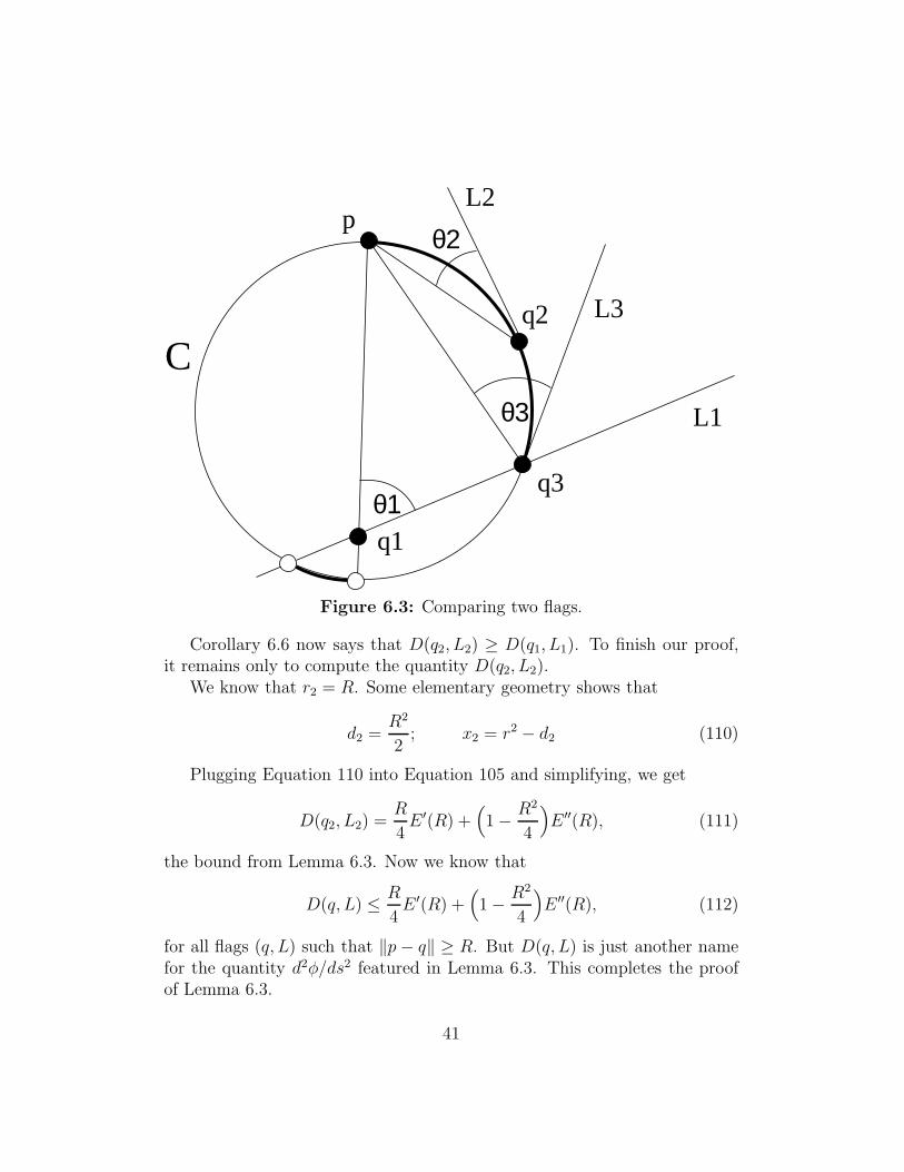
Proof: See Figure 6.3. Let q3 be the endpoint of S such that the smallangle θ1 subtends the arc of C between p and q3, as shown in Figure 6.3.Let L3 be the line tangent to C at q3. Let θ3 = θ(q3, L3). The angle θ1 ishalf the length of the two thick arcs in Figure 6.3 whereas the angle θ3 ishalf thelength of the thick arc joining p to q3. Hence θ3 ≤ θ1. But the angleθ3 decreases as we move q3 towards p along C. Therefore θ2 ≤ θ3. Puttingthese two inequalities together, we find that θ2 ≤ θ1. ♠

40

L1

L3

L2

θ1

q2

p

C

q3

θ2

θ3

q1

Figure 6.3: Comparing two flags.

Corollary 6.6 now says that D(q2, L2) ≥ D(q1, L1). To finish our proof,it remains only to compute the quantity D(q2, L2).

We know that r2 = R. Some elementary geometry shows that

d2 =R2

2; x2 = r2 − d2 (110)

Plugging Equation 110 into Equation 105 and simplifying, we get

D(q2, L2) =R

4E ′(R) +

(1 − R2

4

)E ′′(R), (111)

the bound from Lemma 6.3. Now we know that

D(q, L) ≤ R

4E ′(R) +

(1 − R2

4

)E ′′(R), (112)

for all flags (q, L) such that ‖p− q‖ ≥ R. But D(q, L) is just another namefor the quantity d2φ/ds2 featured in Lemma 6.3. This completes the proofof Lemma 6.3.

41

7 Parametrizing Arcs and Segments

7.1 Overview

Let S ⊂ C be a line segment. In this chapter we define a certain parametriza-tion of S by a parameter x ∈ [0, 1]. Once we define our parametrization, wewill state and prove several geometric results about it. As with the last chap-ter, the reader might want to just note the results on the first reading andthen come back later for the proofs.

Let A be a circular arc on S2, and let A′ be the chord that joins theendpoints A0 and A1 of A. Throughout the chapter, we assume that A iscontained in a semicircle. We let x → A′

x be the affine map from [0, 1] toA′. Let C be the circle containing A, and let c ∈ C be the point which isdiametrically opposed to the midpoint of A. We define Ax so that the threepoints c, A′

x, Ax are always collinear. Here is our first result.

Lemma 7.1 The function f(x) = ‖Ax −A′x‖ attatains its maximum at x =

1/2.

Now we return to our main task of parametrizing a segment S ⊂ C. LetS∗ = Σ−1(S). The method above gives us a parametrization of S∗. Now wedefine

Sx = Σ(S∗x). (113)

As usual Σ denotes stereographic projection.Suppose Q is a normal dyadic square. This means that Q does not cross

the coordinate axes, and the side length of Q is at most 1. We consider thecase when Q is contained in the positive quadrant. The other cases havesymmetric treatments. Let Q0 and Q1 be the left and right edges of Q. Forany x ∈ [0, 1], let Qx denote the segment connecting (Q0)x and (Q1)x. Themain result in this chapter gives estimates on the size and shape of the imageof Q∗

x = Σ−1(Qx).

Lemma 7.2 Q∗x has arc length at most

δ × 1.0013.

and is contained in a circle of radius at least

1√1 + y2

.

42

7.2 Proof of Lemma 7.1

Our result is scale-invariant. It suffices to prove the result when A is an arcof the unit circle, as shown in Figure 7.1. The arc cy is evidently shorterthan the diameter cx. On the other hand, the arc cz is evidently longer thanthe arc cw. Hence the arc yz is shorter than the arc wx. This is what wewanted to prove.

c

z

w x

y

Figure 7.1: The relevant points

7.3 A Lemma about Slopes

The rest of the chapter is devoted to proving Lemma 7.2. Here we reduceLemma 7.2 to a more geometric statement.

Lemma 7.3 Qx has slope in (0, 0.051) for all Q and x ∈ (0, 1).

Proof of Lemma 7.2: Let S = Qx. We deal first with the arc length ofS∗. This is really the same argument as in Lemma 3.4. When evaluated atall points of S, the quantity in Equation 7 is at most δ/s. Since S has slopein (0, 0.051) and Q has side length s, the segment S has length at most

s×√

1 + (0.051)2 < 1.0013. (114)

43

The arc length estimate on S∗ follows by integration.Since the line L through S has positive slope, it intersects the imaginary

axis in a point of the form iy where y < y. But then, according to Equation6, there are two points on (L ∪∞)∗ which are at least

1√1 + y2

apart. ♠

The rest of the chapter is devoted to proving Lemma 7.3.

7.4 Mobius Geometry

Let the vertices of Q be Q00, Q10, Q11, Q01, starting in the bottom left cornerand going counterclockwise around. Associated to Q is an auxilliary mapφ : [0, 1] → [0, 1], defined as follows.

• The point (1 − x)Q00 + xQ01 is (Q0)s for some s.

• The point (Q1)s is (1 − y)Q10 + yQ11 for some y = φ(x).

In other words, we consider the natural map (Q0)s → (Q1)s but we precom-pose and postcompose with affine maps to make the domain and range equalto [0, 1]. Lemma 7.2 is equivalent to the statement that

0 < φ(x) − x < 0.051; ∀x ∈ (0, 1). (115)

Given 4 distinct points A,B,C,D ∈ Rn, we have the cross ratio

χ(A,B,C,D) =‖A− C‖ ‖B −D‖‖A−B‖ ‖C −D‖ . (116)

We say that a homeomorphism from one curve to another is Mobius if themap preserves cross ratios. In case the curves are line segments in the plane,a Mobius map between them is the restriction of a linear fractional transfor-mation of C ∪∞.

Lemma 7.4 φ is Mobius.

44

Proof: Since similarities are Mobius transformations, it suffices to provethat the map (Q0)s → (Q1)s is a Mobius transformation. Stereographicprojection is well known to be a Mobius map from any line segment in C tothe corresponding arc on S2. Referring to the construction in the beginningof §7.1, the map from Ax to A′

x is just the composition of affine maps with(one dimensional) stereographic projection. Hence, this map is also Mobius.

Let A0 = Q∗0 and A′

0 be the chord connecting the endpoints of A0. Like-wise define A1 and A′

1. The map of interest to us is the composition

Q0 → A0 → A′0 → A′

1 → A1 → Q1. (117)

The outer maps are Mobius, from what we have already said, and the middlemap is affine. ♠

A Mobius map from [0, 1] to [0, 1] is completely determined by its deriva-tive at either endpoint. Thus, we can understand φ by computing or esti-mating φ′(0). In our next result, we think of φ′(0) as a function of the choiceof dyadic square Q. As in Equation 7, define

g(x, y) =2

1 + x2 + y2. (118)

Define

GQ =g(Q00)g(Q11)

g(Q10)g(Q10). (119)

Lemma 7.5 Relative to Q, we have

φ′(0) =√GQ.

In particular, φ is the identity iff GQ = 1.

Proof: If follows from symmetry that

φ′(0)φ′(1) = 1. (120)

Therefore

φ′(0) =

√φ′(0)

φ′(1). (121)

45

Looking at the composition in Equation 117, all the maps except the outertwo have the same derivative at either endpoint. For the affine map in themiddle, this is obvious: the derivative is constant. In the case of the mapAj → A′

j this follows from the fact that we are projecting from a point cjthat is symmetrically located with respect to A′

j and Aj. Call this propertyof the derivatives the symmetry property .

By Equation 7, the quantity g(Q00) is the norm of the derivative of Σ−1

at Q00. The other quantities g(Qij) have similar interpretations. It thereforefollows from the symmetry property and the Chain Rule that

φ′(0)

φ′(1)=g(Q00)/g(Q01)

g(Q10)/g(Q11). (122)

This Lemma now follows from Equations 121 and 122. ♠

7.5 The End of the Proof

For the purposes of doing calculus, we define φ and G relative to any squarethat is contained in the positive quadrant. We remind the reader that weonly consider squares that have side length at most 1.

Lemma 7.6 It never happens that GQ = 1.

Proof: When Q00 = (x, y) and Q has side length r, we compute

GQ =(1 + r2 + 2rx+ x2 + y2)(1 + r2 + 2ry + x2 + y2)

(1 + x2 + y2)(1 + 2r2 + x2 + y2 + 2rx+ 2ry)(123)

Every factor in Equation 123 is a polynomial with only constant coefficientsand at least one constant term. Hence this expression never vanishes. ♠

When Q = [0, 1]2, we compute that GQ = 4/3. Hence φ′(0) > 1 relativeto this choice of Q. It tollows from continuity that φ′(0) > 1 relative to anysquare in the positive quadrant. But this means that φ is increasing. (Here,of course, we are crucially using the fact that φ is a Mobius map from [0, 1]to [0, 1].) Hence φ(x) > x. This proves that the slope of the segment Qx ispositive for all Q and all x > 0. This proves half of Lemma 7.3. Now weturn to the other half.

46

Lemma 7.7 The quantity GQ is maximized when Q has side length 1 and

Q00 = (ξ, ξ); ξ =

√3 − 1

2.

Proof: Let ψ(x, y, r) be the function in Equation 123. We compute symbol-ically that

dψ

dr=

∆(x, y, r)

(1 + x2 + y2)2(1 + 2r2 + x2 + y2 + 2rx+ 2ry)2, (124)

Where ∆ is a polynomial with entirely positive terms, at least one of whichinvolves only r. (The polynomial is rather long and unenlightening.) Fromthis we conclude that dψ/dr > 0. Hence, the maximum value of GQ mustoccur when r = 1.

We compute that ψ(ξ, ξ, 1) = 3/2. So, we just have to show that thefunction h(x, y) = 3/2 − ψ(x, y, 1) is non-negative on the positive quadrant.We compute that h is a rational function. The denominator is a polynomialwith only positive terms, and the numerator N equals

1−2x+4x2+2x3+x4−2y−8xy+2x2y+4y2+2xy2+2x2y2+2y3+y4 (125)

In fact, N is non-negative on the entire plane. To see this, we make thechange of variables

x = ξ + u; y = ξ + v. (126)

With this change of variables, we find that N − (2u − 2v)2 is a polynomialinvolving only positive terms. ♠

In light of the previous result, the quantity φ′(0) is maximized for thespecial square Q0 from Lemma 7.7. Since G = 3/2 in this case, we have

φ′(0) =√

3/2. (127)

But this equation pins down φ uniquely, and we observe that the map

φ(x) =3√

2x

2√

3 + 3√x− 2

√3x. (128)

has the same derivative. Hence, this is the correct formula for φ. A bit ofcalculus now shows that

φ(x) − x < 0.051; ∀x ∈ [0, 1]. (129)

This completes the proof.

47

8 Proof of Lemma 5.2

8.1 The Geometry of Circles

We need one more result about circles.

Lemma 8.1 Suppose that A is an arc of a circle C. Let d be the arc-lengthof A. Let A′ be the segment connecting the endpoints of A. Let r be the radiusof C. Let µ be the smallest constant such that every point of A is within µof some point of A′. Then

µ <d2

8r.

Proof: Let’s first consider the case r = 1. We rotate so that C is the unitcircle, and A is the arc bounded by the points exp(−iθ) and exp(iθ). Hereθ ∈ (0, π). Then

d = 2θ; µ = 1 − cos(θ). (130)

The claim of this lemma boils down to the statement that

θ2

1 − cos(θ)> 2, (131)

This is equivalent to the statement that

φ(θ) = θ2 + 2 cos(θ) − 2 > 0. (132)

We have φ(0) = 0 and

φ′(θ) = 2(θ − sin(θ) > 0. (133)

This proves what we need.If r 6= 1, we let T be a dilation that scales distances by a factor of 1/r.

The arc T (A) has length d/r and T (C) has radius 1. We apply our result tothe pair (T (A), T (C)) and find that every point of T (A) is within

(d/r)2

8

of T (C). Applying T−1, we get the desired result for the pair (A,C). ♠

48

8.2 Lemma 5.2 for dyadic segments

8.2.1 Defining the Weighting

Suppose that (Q, Q) is a reasonable pair, and Q is a dyadic line segment.The construction in the previous chapter gives us a parametrization x→ Qx.We take Q0 to be the left endpoint and Q1 to be the right endpoint. Thecorresponding endpoints of Q∗ are Q∗

0 and Q∗1. We define our weighting as

follows. Letting z = Qx, we define

λ0(z) = 1 − x; λ1(z) = x; (134)

8.2.2 Setting up the Calculation

To bring our notation in line with Lemma 6.1, we define

A = A(Q∗0, Q

∗1) = Q∗; A′ = A′(Q∗

0, Q∗1). (135)

Let (z, w) ∈ Q× Q. Define

p = Σ−1(w); q = Σ−1(z). (136)

Setting x = λ1(z), we haveq = Ax. (137)

We also defineq′ = A′

x (138)

The idea of our proof is to estimate things with q′ in place of q, and then toestimate the error we get when replacing q′ by q.

8.2.3 Using Lemma 6.1

Let F be as in Equation 98. We have∑

u

λu(z)f(Qu, w) = (1 − x)F (A′0) + xF (A′

1);

F (A′x) = E(‖q′ − p‖). (139)

Lemma 6.1 now tells us that∑

u

λu(z)f(Qu, w) − E(‖p− q′‖) ≤ max(0,Λ1) δ2 (140)

49

8.2.4 The Easy Case

Now we need to see what happens when we replace q′ by q. Define

r = ‖p− q‖ r′ = ‖p− q′‖. (141)

If r′ ≥ r then (since E is decreasing)

E(‖p− q‖) ≥ E(‖p− q′‖). (142)

In this case, our proof is done: Equations 142 and 140 combine to give atighter bound than what Lemma 5.2 gives.

8.2.5 The Hard Case

Now suppose r′ < r. Since E is convex, E ′ is monotone decreasing. Therefore

E(r′) − E(r) ≤ E ′(r′)‖q − q′‖ ≤ E ′(R)‖q − q′‖. (143)

Here R ≥ r′ is as in Lemma 5.2.The same proof as in Lemma 7.2 shows that A has arc length at most

δ. Also A is contained in a great circle – i.e. a circle of radius 1. Lemma8.1 now says that every point of A is within δ2/8 of A′. But the point of A′

closest to A1/2 is A′1/2. Therefore

‖q − q′‖ = ‖Ax −A′x‖ ≤∗ ‖A1/2 − A′

1/2‖ ≤ δ2

8. (144)

The starred inequality is Lemma 7.1. Combining Equations 143 and 144, wefind that

E(r′) −E(r) ≤ E ′(R)δ2

8= Λ2 δ

2. (145)

Note thatf(z, w) = E(‖p− q‖). (146)

Hence, by Equation 146,

E(‖p− q′‖) − f(z, w) = E(r′) −E(r) ≤ Λ2 δ2. (147)

Adding Equations 140 and 147, we get the bound in Lemma 5.2. This com-pletes the proof in case Q is a dyadic segment.

50

8.3 The Weighting for Dyadic Squares

Let Q be a dyadic square and let Q∗ = Σ−1(Q). Let Qab be the vertices ofQ, as in §7.4. Let Q∗

ab be the corresponding vertex of Q∗. As we make ourconstruction, the reader should picture the letter ‘H’, with the horizontal barvery slightly slanted. We will use coordinates (h, v) ∈ [0, 1]2. The v vari-able moves along vertical segments and the h variable moves along (roughly)horizontal segments.

Let Q0 be the left edge of Q. The two endpoints of Q0 are Q00 and Q01.Likewise, let Q1 be the right edge of Q. The two endpoints of Q10 are Q11.Using the parametrization from the previous chapter, we define

Q0v = (Q0)v ∈ Q0; Q1v = (Q1)v ∈ Q1. (148)

Next, we define Qv to be the segment joining Q0v to Q1v. Note that Qv isnearly horizontal but not exactly horizontal. See Lemma 7.3. Finally, wedefine

Qhv = (Qv)h, (149)

again using the parametrization discussed in the previous sections. We defineour weighting as follows. Assuming that z = Qvh,

λ00(z) = (1 − h)(1 − v); λ10(z) = (h)(1 − v);

λ01(z) = (1 − h)(t); λ11(z) = (h)(v). (150)

In the previous section, we defined a weighting for dyadic segments. Wecould equally well define this weighting for any segment, since we have alreadyexplained how to parametrize any such segment. There are three ways inwhich our weighting here is compatible with the weighting for segments.

• With respect to the segment Q0, the weighting for the point S0v isλ0 = 1 − v and λ1 = v.

• With respect to the segment Q1, the weighting for the point S1v isλ0 = 1 − v and λ1 = v.

• With respect to the segment Qv, the weighting for the point Qhv isλ0 = 1 − h and λ1 = h.

51

8.4 The End of The Proof

For ease of notation, we will assume that our dyadic square lies in the positivequadrant. The other cases are similar, and indeed follow from symmetry. Wegather 4 pieces of information.

1. The circles containing the arcs Q∗0 and Q∗

1 have radius at least

1√1 + x

.

This follows from Equation 6 and from the fact that the line extendinga vertical edge of Q comes within x of the origin.

2. The arcs Q∗0 and Q∗

1 have length at most δ. This follows from the sameargument as in Lemma 7.2.

3. For any v ∈ [0, 1], the line extending the segment Qv comes within yof the origin. Hence, the circle containing Q∗

v has radius at least

1√1 + y

.

See Lemma 7.2.

4. For any v ∈ [0, 1], the arc Q∗v has length at most (1.0013) × δ. See

Lemma 7.2.

Now we are ready for the main argument. The basic idea is to makerepeated appeals to the segment case of Lemma 5.2 and then to suitablyaverage the result.

We defineΛ1x = Λ1y = Λ1/2;

Λ2x = −E′(R)

8

√1 + x2; Λ2y = −E

′(R)

7.98

√1 + y2. (151)

We haveΛ1 = Λ1x + Λ1y; Λ2 = Λ2x + Λ2y. (152)

Let p ∈ (Q)∗ be some point. Let w = Σ(p). Let f be as in Lemma 5.2.That is

f(z, w) = E(‖Σ−1(z) − Σ−1(w)‖). (153)

52

Applying the segment case of Lemma 5.2 to the arc Q0, we find that

Z1 := (1−v)f(Q00, w)+vf(Q01, w)−f(Q0v, w) ≤(

max Λ1x+Λ2x

)δ2 (154)

The proof is exactly the same as in the previous section, except for the onepoint that the circular arc Q∗

0 lies not necessarily in a great circle but rathera circle whose radius is bounded by Item 1 above. The designation Z1 is foralgebraic purposes which will become clear momentarily. Similarly

Z2 := (1−v)f(Q10, w)+vf(Q11, w)−f(Q1v, w) ≤(

max Λ1x+Λ2x

)δ2 (155)

Finally, an argument just like the one given for dyadic segments also worksfor the segment Qs. The only property we used about dyadic segments isthat they don’t cross the coordinate axes, and Qs has this property. UsingItems 3 and 4 above in place of Items 1 and 2, the same argument gives

Z3 := (1−h)f(Q0v, w)+hf(Q1v, w)−f(Qhv, w) ≤(

max Λ1y+Λ2y

)δ2 (156)

The key point here is that

7.98 < 8/1.0013.

The number 1.0013 comes up in Item 4 above.Concentrating on the left hand sides of Equations 154, 155, and 156, we

have(1 − h)Z1 + hZ2 + Z3 =

(1 − h)(1 − v)f(Q00, w) + (1 − h)(v)f(Q01, w)+

(h)(1 − v)f(Q10, w) + (h)(v)f(Q11, w) − f(Qhv, w) =(∑

ab

λab(z)f(Qab, w))− f(z, w); z = Qhv. (157)

Concentrating on the right hand sides, we see that the quantity in Equation157 is at most

(1− h)(

max Λ1x + Λ2x

)δ2 + (h)

(max Λ1x + Λ2x

)δ2 +

(max Λ1y + Λ2y

)δ2 =

(max(Λ1, 0) + Λ2

)δ2. (158)

This proves Lemma 5.2.

53

9 The Hessian and its Variation

9.1 Main Part of the Proof

In this chapter we prove Lemma 2.4. Let He denote the Hessian of E , the en-ergy function, relative to the function E(r) = r−e. Let Z be the configurationcorresponding to the TBP, normalized as in Equation 30.

Lemma 9.1 The lowest eigenvalue of He exceeds 1/10 for e = 1, 2.

Proof: Let M be either of the two matrices. Let I7 be the 7×7 identity ma-trix. Using a modified version of the Cholesky Decomposition, as discussedin [Wa, p 84], we write

(M − 1

10I7) = LDLt. (159)

where L is lower triangular, D is diagonal matrix with all diagonal entriespositive, and Lt is the transpose of L. This suffices to show that M − 1

10I7 is

positive definite. Hence, the lowest eigenvalue of M is at least 1/10. ♠

Given a square matrix M , we define

‖M‖2 =(∑

i,j

M2ij

)1/2

. (160)

We mention a familiar and useful property of this norm.

Lemma 9.2 For any unit vector v ∈ R7 we have ‖M(v) · v‖ ≤ ‖M‖2.

Proof: We have

‖M(v) · v‖2 =∥∥∥

∑Mijvivj

∥∥∥2≤∗ ‖M‖2

∥∥∥∑

(vivj)2∥∥∥

1/2

=

‖M‖2

√(∑v2

i

)(∑v2

j

)= ‖M‖2‖v‖2 = ‖M‖2. (161)

The starred inequality is the Cauchy-Schwarz inequality. ♠

We write M ′ ≺ M if |M ′ij| ≤ Mij for all indices. Recall that s = 2−11, as

in Lemmas 2.3 and 2.4. Let Dk denote the partial derivative with respect tothe kth direction in R7.

54

Lemma 9.3 (Variation Bound) Let Ψ1,e, ...,Ψ7,e be the smallest non-negativematrices such that DkHe(Z) ≺ Ψk,e for all k and all Z ∈ Ωs. Let

Ψ(e) =∥∥∥

7∑

k=1

Ψk,e

∥∥∥2.

Then Ψ(1) < 345 and Ψ(2) < 140 and, supe Ψ(e) < 463.

Corollary 9.4 Let e = 1 or e = 2. Let Z be the center of Ωs (i.e., the TBP)and let W ∈ Ωs be any other point. Then

‖He(Z) −He(W )‖2 <1

10; ∀e ∈ (0,∞).

Proof: Let H = He. Say that a special path in Ω is a 7-segment polygonalpath γ such that the ith segment is parallel to the ith coordinate direction.We can connect Z = Z0 to W = Z7 by a special path γ, all of whosesegments have length at most 2−12. Let Z0, ..., Z7 be the vertices of γ. Let∆ij = H(Zi)−H(Zj). Integrating along the kth segment, we get the bound∆k,k−1 ≺ 2−12Ψk. Hence

‖H(Z) −H(W )‖2 = ‖∆70‖2 =∥∥∥

7∑

k=1

∆k,k−1

∥∥∥2≤

∥∥∥∑7

k=1 Ψk

∥∥∥2

212<

345

4096.

(162)This last quantity is less than 1/10. ♠

Proof of Lemma 2.4: Let e = 1 or e = 2. Let H = He. Let W ∈ Ωs besome point. We want to show that H(W ) is positive definite. Let A = H(Z)and B = H(W ). By the preceding Corollary, we have B = A + ∆ with‖∆‖2 < 1/10.

Now let v ∈ R7 be any unit vector. We have

Bv · v = Av · v + ∆v · v ≥ Av · v − |∆v · v| > 1

10− ‖∆‖2 > 0. (163)

Hence B is positive definite. The fact that Av · v > 1/10 comes from the factthat the lowest eigenvalue of the symmetric matrix A is greater than 1/10. ♠

55

9.2 A Stronger Bound

Consider the functionφ(x) = xe/2 (164)

and the interval

I =

[1

4+

1

2+ 2−9

]. (165)

Define

ck(e) = supx∈I

dkφ

dxk

(x) (166)

Setting ck = ck(e), we define

Υ(e) =√

19336c21 + 19036c1c2 + 4922c22 + 1474c1c3 + 772c2c3 + 31c23. (167)

Our next result uses the notation from the Variation Bound.

Lemma 9.5 (Variation Bound II) Ψ(e) < Υ(e) for all e ∈ (0,∞).

We find easily that

(c1(1), c2(1), c3(1)) = (1, 2, 12). (168)

Plugging this into Equation 167, we get Ψ(1) < 345. Similarly, we have

(c1(2), c2(2), c3(2)) = (1, 0, 0). (169)

This yields Ψ(2) < 140.Some elementary calculus shows that

supe∈(0,∞)

c1(e) < 1.1; supec2(e) < 3.2; sup

e∈(0,∞)

c3(e) < 16. (170)

We omit the details, because we don’t use the general bounds anywhere inour main proof. When we plug in these bounds we find that Ψ(e) < 463 forall e. Hence, the Variation Bound II implies the Variation Bound.

Remark: The Variation Bound II is generally much better than the Varia-tion Bound. For instance, Υ(e) → 0 as e→ 0 or as e→ ∞.

56

9.3 Proof of the Variation Lemma II

Our proof usually suppresses the dependence on the exponent e.A point (z0, z1, z2, z3) ∈ Ωs is such that each zm lies within a square

∆m+1 of side length 2−11 about one of the points of the TBP configuration,normalized as in Equation 30. Let R1 be the union of these 4 squares,∆1, ...,∆4. Let R2 ⊂ C2 denote the set of points z1, z2 which arise as adisjoint pair of finite points of a configuration of Ωs. Here R2 consists of12 components, all of the form ∆i × ∆j . The components ∆i × ∆j and∆j × ∆i are partners. We let ∆5, ...,∆10 be 6 components, no two of whichare partners.

Recall that Σ−1 is inverse stereographic projection. See Equation 5. Set-ting z = x+ iy, define

F (z) =1

‖Σ−1(z) − Σ−1(∞)‖2=

1 + x2 + y2

4. (171)

G(z1, z2) =1

‖Σ−1(z1) − Σ−1(z2)‖2=

(1 + x21 + y2

1)(1 + x22 + y2)

4(x1 − x2)2 + (y1 − y2)2. (172)

Let φ be as in Equation 164. According as m ≤ 4 or m ≥ 5, define

Um = φ Um; Um = F or G (173)

Define

Φ(i, j, k,m) = sup∆m

|DiDjDkUm|; Φ(i, j, k,m) = sup∆m

|DiDjDkUm|. (174)

Here i, j, k ∈ 1, ..., 7 and m ∈ 1, ..., 10 and Dk is the kth partial deriva-tive.

We have

E(z0, z1, z2, z3) =10∑

m=1

Um, (175)

where the arguments of the functions on the right hand side are suitablychosen sub-lists of (z0, z1, z2, z3). Therefore

|DkDiDj(E)| ≤ Ψk(i, j) :=10∑

m=1

Φ(i, j, k,m). (176)

57

With this definition of Ψk, we have DkH ≺ Ψk. Summing over k, we have

∥∥∥7∑

k=1

Ψk

∥∥∥2≤

∥∥∥∑

k,m

Φ(i, j, k,m)∥∥∥

2. (177)

Say that i ∈ 1, ..., 7 is related to an index m ∈ 1, ...., 10 if a change

in the coordinate xi moves one of the points in the argument of Um. Forinstance i = 2 is related to m = 5 because changing x2 changes the locationof the point z1 = x1 + ix2, and the argument of U5 is the point (z0, z1) ∈ ∆5.

Clearly Φ(i, j, k,m) = 0 unless i, j, k are all related to m.When all indices are related to m, we use the chain rule

DiDjDkUm = φ′ ×DiDjDkUm + φ′′′ ×DiUm ×DjUm ×DkUm+

φ′′×DiDjUm×DkUm+φ′′×DjDkUm×DiUm+φ′′×DkDiUm×DjUm. (178)

Given the definitions of the regions R1 and R2 we have Um(∆m) ⊂ I,where I is the interval from Equation 165. Combining this fact with Equation166 and Equation 178, we have

Φ(i, j, k,m) ≤ c1Φ(i, j, k,m) + c3Φ(i,m)Φ(j,m)Φ(k,m)+

c2Φ(i, j,m)Φ(k,m) + c2Φ(j, k,m)Φ(i,m) + c2Φ(k, i,m)Φ(j,m). (179)

Let δm be the center of ∆m. Define

a(i, j, k,m) = |DiDjDkUm(δm)|. (180)

We define a(i, j;m) and a(i;m) similarly. Define

v = ((v(i), v(i, j), v(i, j, k)) =( 1

1000, 0, 0

)or

( 1

200,

1

50,

1

10

), (181)

according as m ≤ 4 or m ≥ 5. Let b(i;m) = a(i;m) + v(i), etc.

Lemma 9.6 for all (i, j, k,m) we have

Φ(i,m) ≤ b(i,m); Φ(i, j,m) ≤ b(i, j,m); Φ(i, j, k,m) ≤ b(i, j, k,m).

58

Combining Equation 177, Equation 179, and Lemma 9.6, we have

∑

k

Ψk ≺∑

k,m

δ(i, j, k,m)

c1b(i, j, k,m)+

c2(b(i, j,m)b(k,m)+

c2(b(j, k,m)b(i,m)+

c2(b(k, i,m)b(j,m)+

c3b(i,m)b(j,m)b(k,m)

(182)

Here δ(i, j, k,m) = 1 if i, j, k are all related to m, and otherwise 0. When wecompute the norm of the right hand side in Mathematica, we get the squareroot of a polynomial in c1, c2, c3. Rounding the coefficients of this polynomialup to integers, we get Υ. This completes the proof of the Variation BoundII, modulo the proof of Lemma 9.6.

9.4 Proof of Lemma 9.6

When m ≤ 4, we are dealing with the function F from Equation 171. Wehave DiF = xi/2 and all higher derivatives are constant. Lemma 9.6 in thistrivial case now follows from the fact that radius(∆m) < 1/500.

For the nontrivial cases, we fix some value of m ∈ 5, ..., 10 and considerthe cube ∆ = ∆m ⊂ C2. This cube has side-length 2−11. The center pointis δ = δm. Define

ak = |DkG(δ)|; Φk = max(z1,z2)∈∆

|DkG(z1, z2)|. (183)

The maxima here are taken over all kth partial derivatives Dk. An exact,finite calculation, done for each of the 6 choices of m, yields

a1 ≤ 1; a2 ≤ 4; a3 ≤ 18; a4 ≤ 96; a5 ≤ 600. (184)

Now we give an estimate on Φ6. Given a polynomial P ∈ R[x1, y1, x2, y2],let |P | denote the sum of the absolute values of the coefficients of P . Wehave the easy upper bound

|P (z1, z2)| ≤ |P |max(|z1|, |z2|)d; d = degree(P ). (185)

59

Here we have set zj = xj + iyj . Calculating symbolically we find that each6th partial derivative D6 has the following structure. There is a polynomialP , depending on the choice of derivative, such that

D6G =P

‖z1 − z2‖7; |P | ≤ 4519440; deg(P ) ≤ 10. (186)

We (easily) have

max(‖z1‖, ‖z2‖, ‖z1 − z2‖−1) < 1 + 2−8; ∀(z1, z2) ∈ ∆. (187)

HenceΦ6 ≤ 4519440 × (1 + 2−8)17 < 5000000. (188)

Lemma 9.7 Φk < ak + 2−10 × Φk+1.

Proof: Let (w1, w2) be a point of ∆. We can connect (w1, w2) to a point(z1, z2) ∈ δ2 by a 4-segment polygonal path γ such that the ith segment haslength at most 2−12 and moves in the ith coordinate direction. This lemmanow follows from integration. ♠

Now we apply Lemma 9.7 in an iterative way.

Φ5 ≤ 600 + 5000000 × 2−10 < 5483 (189)

Φ4 ≤ 96 + 5483 × 2−10 < 102. (190)

|Φ3 − a3| < 102 × 2−10 <1

10; Φ3 < 18.1 (191)

|Φ2 − a2| < 18.1 × 2−10 <1

50; Φ2 < 4.02. (192)

|Φ1 − a1| ≤ 4.02 × 2−10 <1

200. (193)

The R.H.S. of Equation 191 comes from the L.H.S. and Equation 184. Like-wise, the R.H.S. of Equation 192 comes from the L.H.S. and Equation 184.This completes the proof of Lemma 9.6.

60

10 Computational Issues

10.1 General Remarks

Our calculations in this paper are of two kinds. The material in §9 makessome exact calculations in Mathematica [W] and the rest of the paper makescalculations in Java. For the Mathematica calculations, we need to takederivatives of rational functions or their square roots, and evaluate themat elements of Q[

√3]. We also need to simplify and group terms of some

polynomials. Everything is manipulated exactly. The user who downloadsour Java program will also find our Mathematica files in the same directory.

The bulk of the calculations are done in Java, and these are what wediscuss below. We take the IEEE-754 standards for binary floating pointarithmetic [I] as our reference for the Java calculations. This 1985 documenthas recently been superceded by a 2008 publication [I2]. We will stick tothe 1985 publication for three reasons. First, the 1985 version is shorter andsimpler. Second, the portion relevant to our computation has not changed inany significant way. Third, we think that some of the computers running ourcode will have been manufactured between 1985 and 2008, thus conformingto the older standard.

10.2 Doubles

With a view towards explaining interval arithmetic, we first describe the waythat Java represents real numbers. Our Java code represents real numbersby doubles , in a way that is an insignificant modification of the scheme dis-cussed in [I, §3.2.2]. To see what our program does, read the documentationfor the longBitsToDouble method in the Double class, on the websitehttp://java.sun.j2se/1.4.2.docs/api. According to this documentation –and experiments verify that it works this way on our computer – our programrepresents a double by a 64 bit binary string, where

• The first bit is called s.

• The next 11 bits are a binary expansion of an integer e.

• If e = 0, the last 52 bits are the binary expansion of an integer m.

• If e 6= 0, the last 52 bits are binary expansion of the number m− 252.

61

The real number represented by the double is

(−1)s × 2e−1075 ×m. (194)

Example: The double representing −317 is stored as the 64 bit string

1/10000000111/001111010 . . .0.

The slashes are put in to emphasize the breaks. Here s = 1 and (since e 6= 0)

e = 210 + 8 + 4 + 1 = 1031.

There are 44 zeros at the end of the word, and

m = 244(0 + 0 + 32 + 16 + 8 + 4 + 0 + 1) + 252 = 244(317).

Hence(−1)s × 2e−1075 ×m = −317.

Now we come to the main point of our discussion above. The non-negativedoubles have a lexicographic ordering, and this ordering coincides with theusual ordering of the real numbers they represent. The lexicographic orderingfor the non-positive doubles is the reverse of the usual ordering of the realnumbers they represent. To increment x+ of a positive double x is the verynext double in the ordering. This amounts to treating the last 63 bits ofthe string as an integer (written in binary) and adding 1 to it. With thisinterpretation, we have x+ = x+ 1. We also have the decrement x− = x− 1.Similar operations are defined on the non-positive doubles. These operationsare not defined on the largest and smallest doubles, but our program neverencounters (or comes anywhere near) these.

10.3 The Basic Operations

Let D be the set of all doubles. Let

R0 = x ∈ R| |x| ≤ 230 (195)

Our choice of 230 is an arbitrary but convenient cutoff. Let D0 denote theset of doubles representing reals in R0.

According to the discussion in [I, 3.2.2, 4.1, 5.6], there is a map R0 → D0

which maps each x ∈ R0 to some [x] ∈ D0 which is closest to x. In case

62

there are several equally close choices, the computer chooses one accordingto the method in [I, §4.1]. This “nearest point projection” exists on a subsetof R that is much larger than R0, but we only need to consider R0. We alsohave the inclusion r : D0 → R0, which maps a double to the real that itrepresents.

Our calculations use the 5 functions

+; −; ×; ÷;√. (196)

These operations act on R0 in the usual way. Operations with the same nameact on D0. Regarding the first 5 basic operations, [I, §5] states that each ofthe operations shall be performed as if it first produced an intermediate resultcorrect to infinite precision and with unbounded range, and then coerced thisintermediate result to fit into the destination’s format . Thus, for doubles xand y.

√x =

[√r(|x|)

]; x ∗ y = [r(x) ∗ r(y)]; ∗ ∈ +,−,×,÷. (197)

The operations on the left hand side represent operations on doubles and theoperations on the right hand side represent operations on reals.

Remark: Exceptions to Equation 197 can arise if we divide by 0 or a numbertoo close to zero. This will produce an overflow error – too large a numberto be accurately represented by a double. To see that this never happens, wecheck that we never divide by a number smaller than 2−11. Moreover, as wediscuss at the end of this chapter, we never take the square root of a numberless than 2−5.

10.4 Interval Arithmetic

An interval is a pair I = (x, y) of doubles with x ≤ y. Say that I boundsz ∈ R0 if x ≤ [z] ≤ y. This is true if and only if x ≤ z ≤ y. Define

[x, y]o = [x−, y+]. (198)

This operationis well defined for doubles in D0. We are essentially roundingout the endpoints of the interval. Let I0 and I1 denote the left and rightendpoints of I. Letting I and J be intervals, we define

I ∗ J = (minijIi ∗ Ij,max

ijIi ∗ Ij)o;

√I = (

√I0,

√I1)0 (199)

63

That is, we perform the operations on all the endpoints, order the results,and then round outward. Given Equation 197, we have the following facts.

1. If I bounds x and J bounds y then I ∗ J bounds x ∗ y.

2. If I > 0 bounds x > 0 then√I bounds

√x.

After we have defined intervals and their basic operations, we define otherJava objects based on intervals. Namely, interval versions of complex num-bers, vectors in R3, dyadic segments and squares, and dyadic boxes. Forinstance, the interval version of a complex number is an object of the formX + iY , where X and Y are intervals. The algebra of these interval objects– e.g. complex addition or the dot product – is formally the same as thecorresponding algebra on the usual objects. At every step of the calculation,the real version of the object is bounded, component by component, by theinterval version. If some particular interval object passes our test, it meansthat all the real objects bounded by it also pass.

10.5 Implementation Details

We implement the interval arithmetic in a way that tries to minimize thetime we spend using it. We run the floating point algorithm until we noticethat a box has passed one of the floating point tests. Then, we re-performthe interval arithmetic test on the interval arithmetic version of the box.

• If the box passes the interval arithmetic test, we eliminate it, and switchback to the floating point algorithm.

• If the box fails the interval arithmetic test, we just act as if it failedthe corresponding floating point test, and resume the algorithm. Wecall this case a mismatch. It is harmless.

Even though the mismatches are harmless, we prefer to have few mis-matches, so that run time for the interval arithmetic version of the code iseasier to predict from the run time of the floating point version. There are4 kinds of potential mismatches, corresponding to the 4 kinds of tests weperform, as discussed in §2.5. The two mismatches that actually arise (or,rather arose) in abundance are the Energy Estimator mismatches and theRedundancy Eliminator mismatches. Once we make our modifications, the

64

code runs completely without mismatches for the 1/r potential and with onlya 4 mismatches for the 1/r2 potential.

To prevent the Energy Eliminator mismatches, we arrange the floatingpoint eliminator so that a dyadic box passes only if the minimum energy isabove E0+2−40, where E0 is the energy of the T.B.P. In this way, the intervalversions of the boxes that are actually checked have a bit of a cushion. Thereason why this fudge factors does not cause our code to halt is that theinequality E(X)−E0 < 2−40 only occurs well inside the L∞ neighborhood ofsize 2−14 about the TBP.

Adding the fudge factor of 2−40 makes the floating point test harder topass, but does not change the validity of the program. Logically, the float-ing point calculation simply finds a candidate partition of the configurationspace, in which each box in the partition passes one of our tests. Adding thefudge factor does change the final partition a bit, but it doesn’t destroy thebasic property of the partition.

Mismatches occur for the Redundancy Eliminator because we sometimeseliminate configurations where there is an exact equality of coordinates. Thisequality will fail for the corresponding intervals, because of a tiny overlap.To get around this problem, we associate to each dyadic object a Gaussianinteger that represents 225z, where z is the center of the object. When wesubdivide a dyadic object, we perform the arithmetic on the Gaussian integerexactly, so as to compute the exact value of the centers of the subdividedobjects. We never subdivide more than 24 times – and in fact the maximumis about 17 – so we never arrive at a situation where 225z is not an integer.When it comes time to compare the various coordinates of a dyadic object,we actually compare 225 times those coordinates, so that we are working en-tirely with integers. This lets us make exact comparisons.

There is one more fine point we would like to mention. We want to avoidtaking expressions of the form

√I, where I is an interval that is too close to

0. If 0 ∈ I, then I0 < 0 and√I0 causes an arithmetic error. The only time

this issue comes up is in the bounds from Lemma 3.1. The quantity 4 −D2

might be close to 0 if D is close to 2. To avoid this problem, we define a newfunction σ, which has the property σ(I) = 2−5 if I1 < 2−10 and otherwiseσ(I) =

√I. (It never happens that I1 > 2−10 and I0 < 0.) When computing

the interval version of the bound in Lemma 3.1, we use σ in place of√

.This causes no problem with the proof, because the bound is not as strongwhen we use σ in place of

√.

65

11 References

[BBCGKS] Brandon Ballinger, Grigoriy Blekherman, Henry Cohn, NoahGiansiracusa, Elizabeth Kelly, Achill Schurmann,Experimental Study of Energy-Minimizing Point Configurations on Spheres,arXiv: math/0611451v3, 7 Oct 2008

[C] Harvey Cohn, Stability Configurations of Electrons on a Sphere, Math-ematical Tables and Other Aids to Computation, Vol 10, No 55, July 1956,pp 117-120.

[CK] Henry Cohn and Abhinav Kumar, Universally Optimal Distributionsof Points on Spheres , J.A.M.S. 20 (2007) 99-147

[CCD] online website:http://www-wales.ch.cam.ac.uk/∼ wales/CCD/Thomson/table.html

[DLT] P. D. Dragnev, D. A. Legg, and D. W. Townsend, Discrete Loga-rithmic Energy on the Sphere, Pacific Journal of Mathematics, Volume 207,Number 2 (2002) pp 345–357

[HS], Xiaorong Hou and Junwei Shao, Spherical Distribution of 5 Pointswith Maximal Distance Sum, arXiv:0906.0937v1 [cs.DM] 4 Jun 2009

[I] IEEE Standard for Binary Floating-Point Arithmetic (IEEE Std 754-1985) Institute of Electrical and Electronics Engineers, July 26, 1985

[I2] IEEE Standard for Floating-Point Arithmetic (IEEE Std 754-2008) In-stitute of Electrical and Electronics Engineers, August 29, 2008.

[RSZ] E. A. Rakhmanoff, E. B. Saff, and Y. M. Zhou, Electrons on theSphere, Computational Methods and Function Theory, R. M. Ali, St. Ruscheweyh,and E. B. Saff, Eds. (1995) pp 111-127

[SK] E. B. Saff and A. B. J. Kuijlaars, Distributing many points on a Sphere,Math. Intelligencer, Volume 19, Number 1, December 1997 pp 5-11

66

[T] J. J. Thomson, On the Structure of the Atom: an Investigation of theStability of the Periods of Oscillation of a number of Corpuscles arranged atequal intervals around the Circumference of a Circle with Application of theresults to the Theory of Atomic Structure. Philosophical magazine, Series 6,Volume 7, Number 39, pp 237-265, March 1904.

[W] S. Wolfram, The Mathematica Book , 4th ed. Wolfram Media/CambridgeUniversity Press, Champaign/Cambridge (1999)

[Wa] D. Watkins, Fundamentals of Matrix Calculations, John Wiley andSons (2002)

[Y], V. A. Yudin, Minimum potential energy of a point system of charges(Russian) Diskret. Mat. 4 (1992), 115-121, translation in Discrete MathAppl. 3 (1993) 75-81

67