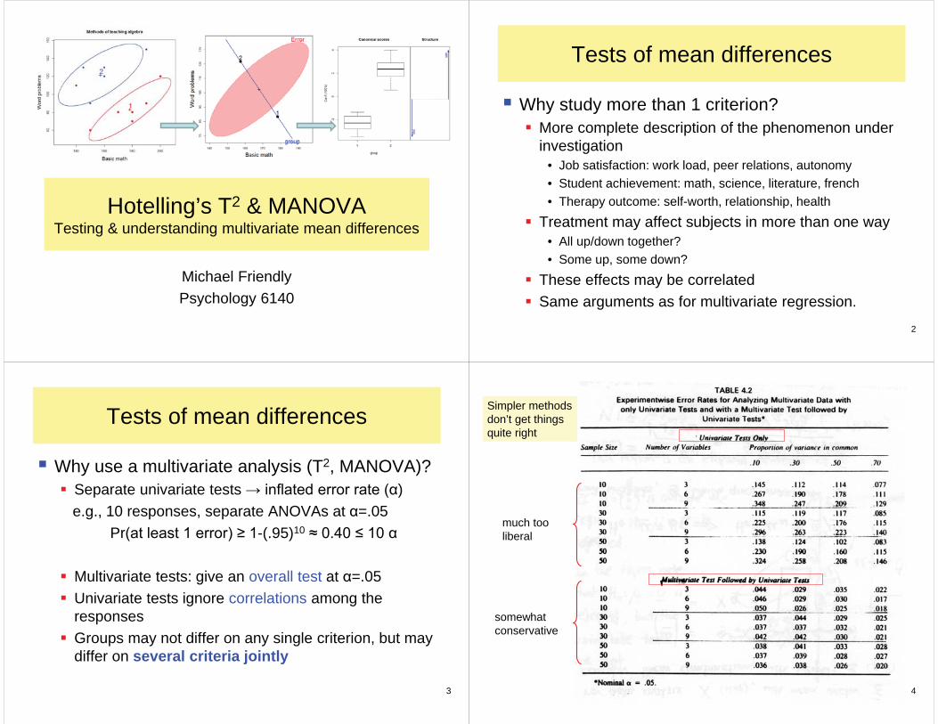
Hotelling’s T2 & MANOVATesting & understanding multivariate mean differences

Michael FriendlyPsychology 6140

2

Tests of mean differences

Why study more than 1 criterion?More complete description of the phenomenon under investigation

• Job satisfaction: work load, peer relations, autonomy• Student achievement: math, science, literature, french• Therapy outcome: self-worth, relationship, health

Treatment may affect subjects in more than one way• All up/down together?• Some up, some down?

These effects may be correlatedSame arguments as for multivariate regression.

3

Tests of mean differences

Why use a multivariate analysis (T2, MANOVA)?Separate univariate tests )

e.g., 10 responses, separate ANOVAs at =.05 Pr -(.95)10

Multivariate tests: give an overall test at =.05Univariate tests ignore correlations among the responsesGroups may not differ on any single criterion, but may differ on several criteria jointly

4

much too liberal

somewhat conservative

Simpler methods don’t get things quite right

5

Tests of mean differences

Why not always use MANOVA tests?Like overall F-test in ANOVA---

• Many responses, small effects test on all responses.

• As usual, hypothesis tests should be focused on research questions, rather than “shotgun” approach

Somewhat harder to describe / explain• Multiple test statistics: Wilks’, HLT, Pillai, Roy• But: all are equivalent for s=1 tests, so no problem• just report the equivalent F (all the same for T2 here)

6

Hotelling’s T2

Multivariate generalization of univariate t-testt-test :: ANOVA as T2 :: MANOVA

T2 as maximum univariate t2 for a linear combination of responsesSpecial case of the GLH: L B M = 0Introduces ideas of discriminant analysisIntroduces ideas of MANOVA

In the history of multivariate statistical methods, there are a few important ideas that paved the way from univariate

7

T2: generalized t test

1 sample, univariateH0 : = 0

H1 : 0

1 sample, multivariateH0 : = 0 (p x 1)

H1 : 0

0 )(s

x Nt

22 2 10

0 02

( ) ( )( ) ( )N x N x s xs

t

2 10 0( ) ( )NT x

Squared distance between mean vector and hypothesis, in the metric of S -1

Thus, T2 is like the square of a univariate t statistic

T2: generalized t test

8

2 10 0

20( )

( ) ( )

,

NT

N D

xx

Squared distance between mean vector and hypothesis, in the metric of S -1

Q: For the same means, would T2 be larger or smaller if r < 0?

01

02

1

2

x

x

t1

t2

T

x1: anxiety

x2: depression

Does exam period increase anxiety anddepression?

10

T2: max possible t2 for linear combination

For data matrix X(n x p), consider linear comb with weights a(p x 1) :

w = X aThen H0 : = 0 (p x 1) 0 : w = a’ 0

Find weights to give max t2:

02

( () )/

w

w

t s Nws N

aaa'Sa

0 0[ ( )( )'(

] 00r, )o H E

N xQQ a

Rank (QH)=1 -zero latent root11

T2: max possible t2 for linear combination

Hence, the maximum value of t2(a) is

The corresponding latent vector, a, is

(raw) discriminant function coefficients. These give the relative contribution of each response to T2

In the two-sample case, analogous results using

1 20 0' )( () TN x S x

10( )a S x

1 2( )x x

(the 1 non-zero latent root)

12

T2: critical values

For a single response, t2N-1 ~ F(1,N-1)Since we chose a to give max t2(a), need to take this into account.Hotelling showed that a transformation of T2 hasan F distribution

In SAS/SPSS/R, we typically use equivalent F values based on Roy’s test or HLT

2T ~ ( , )( 1)N p F p N p

p NF

13

T2: invariance

Univariate t unchanged under any lineartransformation

xT2 is invariant under all affine transformationsx (p x 1) C (p x p) x + d : C non-singular

The same is true for all MANOVA tests

14

T2: confidence regions for meansA 1- confidence region for (p x 1) consists of those for which

11

( 1)( ' ) )) ( ( ,p Nx S x FN p

N p N pData ellipse centered at means

In the figure, note that H0: = 0 is rejected, but the univariatetests are not rejected.

Convert F back to T2

15

T2: special case of GLM

The multivariate General Linear Model expresses all models in the form

n p n q q p n pY X B EA two-sample T2 takes the form:

(ˆ '

ˆ

' )1

2

B X X' X

'

YThe usual LS estimates:

16

T2: special case of GLH

All hypotheses are of the form

Eg H0: 1 = 2 1 – 2 = 0

0 :H L B M 0Contrasts among groups

Contrasts among variables (profile analysis)

1 3 3

2

(0 1 1) ''

'LBM 0

17

Example: methods of teaching algebra

Responses: students evaluated on--Basic math (BM)Word problems (WP)

Groups: two instructors, different teaching methods (presumably: equal ability, random assignment)

18

title 'Two-Sample Hotelling T2'; data mathscor; input group BM WP; label BM='Basic Math' WP='Word Problems'; datalines; 1 190 90 1 170 80 1 180 80 1 200 120 1 150 60 1 180 70 2 160 120 2 190 150 2 150 90 2 160 130 2 140 110 2 145 130 ;

1 190 901 170 801 180 801 200 1201 150 601 180 702 160 1202 190 1502 150 902 160 1302 140 1102 145 130

t p-valueBM 2.06 0.066WP -3.23 0.009**

Univariate tests

19

proc gglm data=mathscor outstat=HEstats; class group; model BM WP = group / nouni; manova H=group; run;

MANOVA Test Criteria and Exact F Statistics for the Hypothesis of No Overall group Effect H = Type III SSCP Matrix for group E = Error SSCP Matrix S=1 M=0 N=3.5 Statistic Value F Value Num DF Den DF Pr > F Wilks' Lambda 0.13481891 28.88 2 9 0.0001 Pillai's Trace 0.86518109 28.88 2 9 0.0001 Hotelling-Lawley Trace 6.41735719 28.88 2 9 0.0001 Roy's Greatest Root 6.41735719 28.88 2 9 0.0001

T2 = dfe x 1 = (n1 + n2 -2) x HLT = 10 HLT = 64.17

All F values are equal when s = dfh = 1

2 = 1 – = 0.865

20

> mod <- lm(cbind(BM, WP) ~ group, data=mathscore)> Anova(mod)

Type II MANOVA Tests: Pillai test statisticDf test stat approx F num Df den Df Pr(>F)

group 1 0.86518 28.878 2 9 0.0001213 ***---Signif. codes: 0 ‘***’ 0.001 ‘**’ 0.01 ‘*’ 0.05 ‘.’ 0.1 ‘ ’ 1>> print(summary(Anova(mod)), SSP=FALSE)

Type II MANOVA Tests:------------------------------------------

Term: group Multivariate Tests: group Df test stat approx F num Df den Df Pr(>F) Pillai 1 0.8652 28.878 2 9 0.0001213 ***Wilks 1 0.1348 28.878 2 9 0.0001213 ***Hotelling-Lawley 1 6.4174 28.878 2 9 0.0001213 ***Roy 1 6.4174 28.878 2 9 0.0001213 ***---Signif. codes: 0 ‘***’ 0.001 ‘**’ 0.01 ‘*’ 0.05 ‘.’ 0.1 ‘ ’ 1

Analysis with R:

21

Visualizing T2 & MANOVA

Data ellipses show:• group means (centroids)• within-group scatter• (are they ~ the same?)

covEllipses(mathscore[,2:3], mathscore$group, pooled=FALSE)

Interpretation: Instructor 1 focuses more on Basic Math; instructor 2 on Word Problems

This bivariate display is much more informative than separate univariate displays for BM and WP!

22

Visualizing T2 & MANOVA

HE plots show:• variation of means (H)• pooled within-group scatter (E)

heplot(mod, fill=TRUE, xlab="Basic math", ylab="Word problems")

23

Visualizing T2 & MANOVA

Overlaying these shows:• variation of means (H)• pooled within-group scatter (E)= average of within-group var-cov matrices• discriminant axis = H

Discriminant analysis:

• Find linear comb of BM, WP to best discriminate between groups

• DA also allows different n s of groups and cost of mis-classification (shifts boundary line)

24

Assumptions: homogeneity of (co)variance

For univariate t-test or ANOVA, we assume equal variance within groups

s21 = s2

2 = …= s2g

2pooled or MSE

Box test or Levine’s test often usedMultivariate tests: translates to equality of within-group covariance matrices,

S1 = S2 = …= Sg pooled = E matrixBox M test: H0 : 1 = 2 = …= g

SAS: proc discrim, pool=test optionWhy: discriminant function is linear of S1 = S2 = ... but quadratic otherwiseR: heplots::boxM()

/2

/2| || | iN

iNpooled

MS

S2 with (g-1)p(p+1)/2 df

25

pproc ddiscrim data=mathscor pool=test canonical ncan=11 out=scores; class group; var BM WP;

The DISCRIM Procedure Test of Homogeneity of Within Covariance Matrices Chi-Square DF Pr > ChiSq 0.617821 3 0.8923

Raw Canonical Coefficients Variable Can1 BM -0.0835 WP 0.0753

group BM WP Can1 1 190 90 -2.78495 1 170 80 -1.86756 1 180 80 -2.70261 1 200 120 -1.36188 1 150 60 -1.70287 1 180 70 -3.45531 2 160 120 1.97832 2 190 150 1.73129 2 150 90 0.55525 2 160 130 2.73102 2 140 110 2.89571 2 145 130 3.98360

(I’m using this as a short cut to also introduce canonical analysis)

26

T2 = t2 based on Can1

proc tttest data=scores; class group; var can1; run;

T-Tests Variable Method Variances DF t Value Pr > |t| Can1 Pooled Equal 10 -8.01 <.0001 Can1 Satterthwaite Unequal 8.8 -8.01 <.0001

T2 = (-8.01)2 = 64.17

A simple t test using canonical scores is equivalent to Hotelling’s T2

27

Canonical analysis in R with the candisc package

library(candisc)mod.can <- candisc(mod)summary(mod.can)

Canonical Discriminant Analysis for group:

CanRsq Eigenvalue Difference Percent Cumulative1 0.8652 6.417 100 100

Class means:[1] -2.313 2.313

std coefficients:BM WP

-1.463 1.546

plot(mod.can)

boxM(mod) Box's M-test for Homogeneity of Covariance Matrices

Chi-Sq (approx.) = 0.618, df = 3, p-value = 0.89

28

Example: Delay in oral practice

Postovsky (1970): Two groups were studied in second language learning (n=28 each)

Control: 0 delay before starting oral practiceExpt’l: 4 week delay before starting oral practiceNB: groups were matched on age, education, former language training & language aptitude [Why?]

Responses (exam after 6 weeks):listenspeakreadwrite

29

data oral; input subjno grp listen speak read write; length Group $ 88; if grp=11 then Group='Exptl'; if grp=22 then Group='Control'; datalines; 1 1 34 66 39 97 2 1 35 60 39 95 3 1 32 57 39 94 4 1 29 53 39 97 5 1 37 58 40 96 6 1 35 57 34 90 7 1 34 51 37 84 8 1 25 42 37 80 ...

1 1 34 66 39 972 1 35 60 39 953 1 32 57 39 944 1 29 53 39 975 1 37 58 40 966 1 35 57 34 907 1 34 51 37 848 1 25 42 37 80

Complete output on class web: SAS examples/glm/oral.sas

30

pproc gglm data=oral outstat=HEstats; class group; model listen--write = group; manova h = group / short; run;

MANOVA Test Criteria and Exact F Statistics for the Hypothesis of No Overall Group Effect H = Type III SSCP Matrix for Group E = Error SSCP Matrix S=1 M=1 N=24.5 Statistic Value F Value Num DF Den DF Pr > F Wilks' Lambda 0.914414 1.19 4 51 0.3250 Pillai's Trace 0.085586 1.19 4 51 0.3250 Hotelling-Lawley 0.093596 1.19 4 51 0.3250 Roy's Greatest Root 0.093596 1.19 4 51 0.3250

2 = 1 – = 0.086 NB: s = min(p, dfh), where dfh=g-1

oral.mod <- lm(cbind(listen, speak, read, write) ~ Group, data=oral)Anova(mod) 31

Visualizing the analysis

HE plot shows that:

• Exptl > Control on both measures

• Diffce too small, relative to error variation, to be considered significant

• Residuals are also positively correlated

• The H “ellipse” becomes a line when s=1

heplot(oral.mod, fill=TRUE)

32

HE plot matrix confirms that this is true for all pairs of responses

pairs(oral.mod, fill=TRUE, ...)

33

Profile analysis (repeated measures)

When the responses are commensurate (on the same scale) it is often useful to test equal means acrossresponsesUnivariate analysis (repeated measures) and multivariate analysis (profile analysis) frame similar questions, in different ways

Parallel profiles: No Group x Measure interactionEqual levels: No Group main effectFlatness: No Measure main effect

Univariate analysis relies on additional assumptions (compound symmetry), not always met in data

34

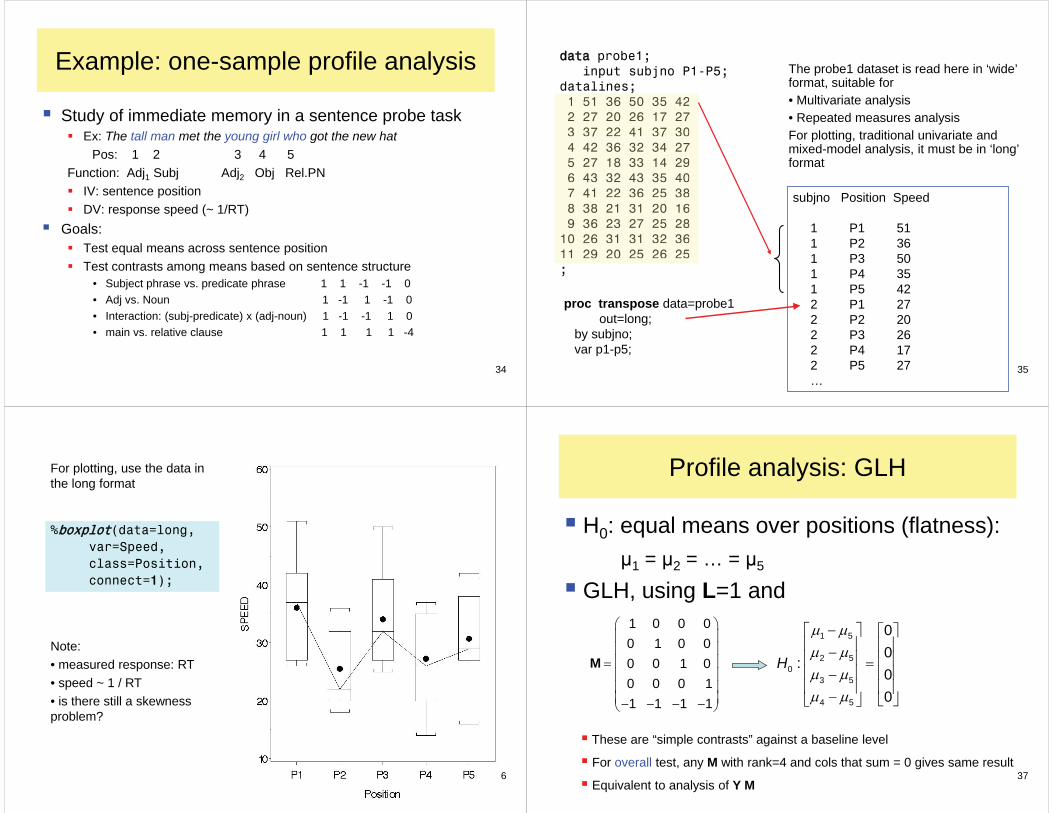
Example: one-sample profile analysis

Study of immediate memory in a sentence probe taskEx: The tall man met the young girl who got the new hat

Pos: 1 2 3 4 5Function: Adj1 Subj Adj2 Obj Rel.PN

IV: sentence positionDV: response speed (~ 1/RT)

Goals:Test equal means across sentence positionTest contrasts among means based on sentence structure

• Subject phrase vs. predicate phrase 1 1 -1 -1 0• Adj vs. Noun 1 -1 1 -1 0• Interaction: (subj-predicate) x (adj-noun) 1 -1 -1 1 0• main vs. relative clause 1 1 1 1 -4

35

ddata probe1; input subjno P1-P5; datalines; 1 51 36 50 35 42 2 27 20 26 17 27 3 37 22 41 37 30 4 42 36 32 34 27 5 27 18 33 14 29 6 43 32 43 35 40 7 41 22 36 25 38 8 38 21 31 20 16 9 36 23 27 25 28 10 26 31 31 32 36 11 29 20 25 26 25 ;

1 51 36 50 35 422 27 20 26 17 273 37 22 41 37 304 42 36 32 34 275 27 18 33 14 296 43 32 43 35 407 41 22 36 25 388 38 21 31 20 169 36 23 27 25 2810 26 31 31 32 3611 29 20 25 26 25

The probe1 dataset is read here in ‘wide’ format, suitable for• Multivariate analysis• Repeated measures analysisFor plotting, traditional univariate and mixed-model analysis, it must be in ‘long’ format

proc transpose data=probe1 out=long; by subjno; var p1-p5;

subjno Position Speed

1 P1 51 1 P2 36 1 P3 50 1 P4 35 1 P5 42 2 P1 27 2 P2 20 2 P3 26 2 P4 17 2 P5 27 …

36

%bboxplot(data=long, var=Speed, class=Position, connect=11);

For plotting, use the data in the long format

Note:• measured response: RT• speed ~ 1 / RT• is there still a skewness problem?

37

Profile analysis: GLH

H0: equal means over positions (flatness):1 = 2 = … = 5

GLH, using L=1 and 1 0 0 00 1 0 00 0 1 00 0 0 11 1 1 1

M

1 5

50

5

5

2

3

4

00

:00

H

These are “simple contrasts” against a baseline level

For overall test, any M with rank=4 and cols that sum = 0 gives same result

Equivalent to analysis of Y M

38

proc glm data=probe1; model P1-P5 = / nouni; manova H= intercept ; /* No position effect*/

MANOVA Test Criteria and Exact F Statistics for the Hypothesis of no POSITION Effect H = Type III SSCP Matrix for POSITION E = Error SSCP Matrix S=1 M=1 N=2.5 Statistic Value F Value Num DF Den DF Pr > F Wilks' Lambda 0.248225 5.30 4 7 0.0277 Pillai's Trace 0.751775 5.30 4 7 0.0277 Hotelling-Lawley 3.028595 5.30 4 7 0.0277 Roy's Greatest Root 3.028595 5.30 4 7 0.0277

Complete output on class web: SAS examples/glm/probe1.sas

probe1.mod <- lm(cbind(p1, p2, p3, p4, p5) ~ 1, data=probe1)idata <- data.frame(position=factor(1:5))Anova(probe1.mod, idata=idata, idesign = ~ position)

In R:

39

The same hypothesis can be tested using the repeated statement:

proc glm data=probe1; model P1-P5 = / nouni; repeated Position 5 contrast(5);

In addition to the multivariate test, we get the traditional univariate tests. However, these rely on additional assumptions (more later).

Repeated Measures Analysis of Variance Univariate Tests of Hypotheses for Within Subject Effects

Adj Pr > FSource DF SS Mean Sq F Value Pr > F G – G H - F

POSITION 4 867.527 216.881 9.25 <.0001 0.0001 <.0001Error(POSITION) 40 938.072 23.452

Greenhouse-Geisser Epsilon 0.7851Huynh-Feldt Epsilon 1.1860

40

Profile analysis: GLH contrasts

Here, we also want to test specific contrasts among the sentence positions

In proc glm, any custom M can be defined in the manova statement

1

2

1 1 1 11 1 1 11 1 1 11 1 1 10 0 0 4 Re

AdjSubjAdjObj

l

M

41

pproc gglm data=probe1; model P1-P5 = / nouni; manova H= intercept /* No position effect */ M= P1 + P2 - P3 - P4, /* Subject vs. Predicate */ P1 - P2 + P3 - P4, /* Adjs vs Nouns */ P1 - P2 - P3 + P4, /* SubPred x AdjNoun */ P1 + P2 + P3 + P4 - 44*P5 /* Relative clause */ mnames = SubjPred AdjNoun SPxAN RelPN / summary printH printE SHORT ;

M Matrix Describing Transformed Variables P1 P2 P3 P4 P5 SUBPRED 1 1 -1 -1 0 ADJNOUN 1 -1 1 -1 0 SPxAN 1 -1 -1 1 0 RELPN 1 1 1 1 -4

42

H & E matrices

E = Error SSCP Matrix SUBPRED ADJNOUN SPxAN RELPN SUBPRED 694.18 54.91 23.82 562.72 ADJNOUN 54.91 1370.55 -48.91 53.64 SPxAN 23.82 -48.91 482.18 863.27 RELPN 562.72 53.64 863.27 6026.91

694.18 1370.55

482.18 6026.91

H = Type III SSCP Matrix for Intercept SubjPred AdjNoun SPxAN RelPN SubjPred 0.82 52.09 11.18 0.27 AdjNoun 52.09 3316.45 711.91 17.36 SPxAN 11.18 711.91 152.82 3.73 RelPN 0.27 17.36 3.73 0.09

0.82 3316.45

152.82 0.09Diag elements

are univariate SS for each contrast

H is labeled ‘Intercept’ since H0 is mean=0

43

Multivariate Analysis of Variance Dependent Variable: SUBPRED Source DF Type III SS Mean Square F Value Pr > F Intercept 1 0.81818 0.8181818 0.01 0.9157 Error 10 694.18182 69.4181818 Dependent Variable: ADJNOUN Source DF Type III SS Mean Square F Value Pr > F Intercept 1 3316.4545 3316.454545 24.20 0.0006 Error 10 1370.5456 137.054545 Dependent Variable: SPxAN Source DF Type III SS Mean Square F Value Pr > F Intercept 1 152.81818 152.8181818 3.17 0.1054 Error 10 482.18182 48.2181818 Dependent Variable: RELPN Source DF Type III SS Mean Square F Value Pr > F Intercept 1 0.0909 0.090909 0.00 0.9904 Error 10 6026.9091 602.690909

F Value Pr > F 24.20 0.0006

So, these are based on the diag elements of H and E

44

Two-sample profile analysis

Same probe task, but with two groups:Gp 1: low STM capacityGp 2: high STM capacity

Questions:Are profiles parallel? (Group x Position)Equal levels? (Group main effect)Flat profiles? (Position main effect)

45

Two-sample profile analysis: GLH

Parallelism:

L = (1 -1)

11 12 21 22

12 13 22 2301

13 14 23 24

14 15 24 25

:H

1 0 0 01 1 0 00 1 1 00 0 1 10 0 0 1

Mcontrast for groups

profile contrasts for positions

Interaction of Group x Position:

are successive differences the same for Gp 1 & 2?

46

Two-sample profile analysis: GLH

Equal levels (Group effect)H0: 1 = 2 1’ 1 – 1’ 2 = 0 (in univariate tests)GLH:

L = (1 -1) M = I(5x5)

Flatness (Position effect)H0: ( 11+ 21)= … = ( 15+ 25)GLH:

L = (1 1)

1 0 0 01 1 0 00 1 1 00 0 1 10 0 0 1

M

47

proc glm data=probe2; class group; model p1-p5 = group / nouni; repeated position 5 profile / short; manova h = group / printe printh short; title2 'Two Sample Profile Analysis'; run;

Statistic Value F Value Num DF Den DF Pr > F Wilks' Lambda 0.21986 13.31 4 15 <.0001 Pillai's Trace 0.78013 13.31 4 15 <.0001 Hotelling-Lawley 3.54825 13.31 4 15 <.0001 Roy's Greatest Root 3.54825 13.31 4 15 <.0001

Statistic Value F Value Num DF Den DF Pr > F Wilks' Lambda 0.83906 0.72 4 15 0.5919 Pillai's Trace 0.16094 0.72 4 15 0.5919 Hotelling-Lawley 0.19181 0.72 4 15 0.5919 Roy's Greatest Root 0.19181 0.72 4 15 0.5919

Position effect:

Position x Group effect:

repeated measures tests (univariate)

multivariate tests

48

Repeated Measures Analysis of Variance Tests of Hypotheses for Between Subjects Effects Source DF SS Mean Square F Value Pr > F group 1 1772.41 1772.4100 8.90 0.0080 Error 18 3583.14 199.0633

Statistic Value F Value Num DF Den DF Pr > F Wilks' Lambda 0.55608 2.24 5 14 0.1083 Pillai's Trace 0.44392 2.24 5 14 0.1083 Hotelling-Lawley 0.79832 2.24 5 14 0.1083 Roy's Greatest Root 0.79832 2.24 5 14 0.1083

Group effect: H0: 1 = 2

Compare with univariate, repeated measures approach: 1’ 1 – 1’ 2=0

The univariate test looks at only one contrast among the many tested by the multivariate test.

49

Repeated Measures Analysis of Variance Univariate Tests of Hypotheses for Within Subject Effects Adj Pr > F Source DF SS MS F Value Pr > F G - G H - F position 4 3371.30 842.825 14.48 <.0001 <.0001 <.0001 position*group 4 79.94 19.985 0.34 0.8479 0.8068 0.8479 Error(position) 72 4191.96 58.222 Greenhouse-Geisser Epsilon 0.8009 Huynh-Feldt Epsilon 1.0487

Univariate, repeated measures tests rely on further assumption:• Compound symmetry (= correlations among repeated measures)• Univariate adjustments (G-G, H-F) adjust the p-values to take violations into account

Complete output on class web: SAS examples/glm/probe2.sas

50

proc transpose data=probe2 out=long; var p1-p5; by group subjno; run;data long; set long; rename col1=Speed _name_=Pos; label _name_='Position'; run;

%meanplot(data=long, var=Speed, class=Pos Group);

Plotting means: %meanplot

Reshape data to long format:

51

HE plots

1

2

1 1 1 11 1 1 11 1 1 11 1 1 10 0 0 4 Re

AdjSubjAdjObj

l

M

Using substantive contrasts for the sentence positions:

HE plot shows the position effect is mainly in the Adj vs Noun contrast

52

Summary

Hotelling’s T2 introduces general ideas:T2: multivariate analog of t2

Special case of GLH for 1- & 2-sample designT2 ~ 1

Multiple groups: t-test :: ANOVA as T2 :: MANOVASpecific tests: contrasts among groups (L) and among responses (M) – better than all pairwise!Visualizing hypothesis and error variation via HE plots

• 1 df tests: H “ellipse” is a line• Orientation: Shows variation of means wrt responses